Weighted regularization for composite materials in electromagnetism

Mathematical Modelling and Numerical Analysis Will be set by the publisher

Modelisation Mathematique et Analyse Numerique

WEIGHTED REGULARIZATION FOR COMPOSITE MATERIALS IN

ELECTROMAGNETISM

Patrick Ciarlet, Jr.1, Francois Lefevre2, Stephanie Lohrengel2 and Serge

Nicaise3

Abstract. In this paper, a weighted regularization method for the time-harmonic Maxwell equationswith perfect conducting or impedance boundary condition in composite materials is presented. Thecomputational domain Ω is the union of polygonal or polyhedral subdomains made of different materi-als. As a result, the electromagnetic field presents singularities near geometric singularities, which arethe interior and exterior edges and corners. The variational formulation of the weighted regularizedproblem is given on the subspace of H(curl; Ω) whose fields u satisfy wα div(εu) ∈ L2(Ω) and havevanishing tangential trace or tangential trace in L2(∂Ω). The weight function w(x) is equivalent to thedistance of x to the geometric singularities and the minimal weight parameter α is given in terms ofthe singular exponents of a scalar transmission problem. A density result is proven that guarantees theapproximability of the solution field by piecewise regular fields. Numerical results for the discretizationof the source problem by means of Lagrange Finite Elements of type P1 and P2 are given on uniformand appropriately refined two-dimensional meshes. The performance of the method in the case ofeigenvalue problems is adressed.

Resume. Dans cet article, nous presentons une approche de type regularisation a poids pour resoudreles equations de Maxwell harmoniques en temps, avec condition aux limites de conducteur parfait oud’impedance. Le domaine de calcul Ω est la reunion de sous-domaines polygonaux ou polyedriquescontenant des milieux materiels differents. Le champ electromagnetique produit est par voie deconsequence singulier au voisinage des singularites geometriques, formees des aretes et coins exterieurset interieurs. La formulation variationnelle de type regularisation a poids est construite dans un sous-espace de H(curl; Ω), dont les elements u sont tels que wα div(εE) appartienne a L2(Ω), avec unetrace tangentielle dans L2(∂Ω) eventuellement nulle. Le poids w(x) considere se comporte comme ladistance de x aux singularites geometriques, alors que l’exposant minimal α est determine en fonctiondes exposants singuliers d’un probleme de transmission scalaire. Nous demontrons un resultat de den-site garantissant l’approximabilite du champ cherche par des champs reguliers par morceaux. Nouspresentons ensuite des resultats numeriques sur le probleme source, obtenus a l’aide d’Elements Finisde Lagrange P1 et P2 sur des maillages bidimensionnels uniformes ou raffines. Nous evaluons enfin laperformance de la methode sur le probleme aux valeurs propres, avec le meme type de discretisation.

1991 Mathematics Subject Classification. 78M10, 65N30, 78A48.

Keywords and phrases: Maxwell’s equations, interface problem, singularities of solutions, density results, weighted regularization

1 Laboratoire POEMS, UMR 7231 CNRS/ENSTA/INRIA, ENSTA ParisTech, 32, boulevard Victor, 75739 Paris Cedex 15,France; e-mail: [email protected] Laboratoire de Mathematiques, FRE 3111, UFR Sciences exactes et naturelles, Universite de Reims Champagne-Ardenne,Moulin de la Housse - B.P. 1039, 51687 Reims Cedex 2, France;e-mail: [email protected] & [email protected] LAMAV, Universite de Valenciennes et du Hainaut Cambresis, Le Mont Houy, 59313 Valenciennes Cedex 9, France;e-mail: [email protected].

c© EDP Sciences, SMAI 1999

2

The dates will be set by the publisher.

1. Introduction

The question of approximability of the solution of Maxwell’s equations by means of nodal finite elementshas been widely studied in the last ten years (see e.g. [2, 4, 5, 10, 18, 32] for perfect conducting boundary con-ditions and homogeneous materials). In a regular domain of class C1 as well as in a convex polyhedron, thediscretization of the time-harmonic Maxwell equations can be performed via standard Lagrange Finite Elementsby solving an equivalent regularized variational formulation similar to the vector Helmholtz equation (see [25]).In a non-convex polyhedron, however, this approximation fails since the electromagnetic field does in generalpresent singularities near the reentrant edges and corners (see e.g. [7, 8, 17]) and the discretization space is nolonger dense in the vector space of the variational formulation. The same situation does occur in compositematerials where the electric permittivity and the magnetic permeability are piecewise constant functions. Theelectromagnetic field then presents singularities near the exterior and interior edges and corners of the differentsubdomains [19].

In order to overcome the lack of density, several possibilities have been studied. The singular complementmethod [3] and singular field method [26] add explicitly the singularities to the discretization space according tothe splitting of the electromagnetic field into a regular part and a singular part deriving from a scalar potential.Another possibility is the penalization of the perfect conducting boundary condition by an impedance-likecondition. From a theoretical point of view, the density result of the FE-space in the variational space holdstrue for any homogeneous material (see [13, 16]) and some composite materials (see [29]). The numericalperformances of this method, however, are rather poor. The idea of weighted regularization has been developedin [18] for homogeneous materials. It consists in looking for the solution in the subspace of H(curl; Ω) offields with divergence in a weighted L2-space, whereas the classical regularized formulation corresponds to theL2-space without weight.

In this paper, we study the method of weighted regularization for composite materials and prove the density ofthe space of piecewise regular vector fields in the space of the weighted regularization method, for an appropriatechoice of the weight parameter. The idea of the proof is similar to the proof in [29] where the case of classicalregularization with impedance boundary condition has been addressed. It consists in proving that the orthogonalof the closure of the space of piecewise regular vector fields is reduced to 0. However, if the density resultfor classical regularization with impedance boundary condition always holds true in the case of homogeneousmaterials, it may fail for some composite materials. On the contrary, the method of weighted regularizationallows one to choose the weight parameter depending on the singularities of a scalar second-order transmissionproblem and hence, the density result may be recovered for any composite material.

The paper is organized as follows: the theoretical aspects of the problem are dealt with in section 2. Moreprecisely, in §2.1, we give the geometric setting and the functional framework including a perfect conductingboundary as well as an impedance boundary condition. We also address equivalence between the weightedregularized formulation and the original Maxwell equations. In §2.2, we show that the density problem forvector fields can be reduced to a similar density problem for the associated scalar potentials. The weightfunction in two dimensions will be defined in §2.3. The proof of the density result in a two-dimensional domainis developed for a more general family of two-dimensional scalar problems depending on a real parameter. Thisturns out to be useful in order to deal with the three-dimensional case where the real parameter representsthe (local) edge variable. Subsection 2.4 is devoted to the proof of the density result in a polyhedron. Insection 3, we state precisely the discretization by means of Lagrange Finite Elements of type Pk and give abasic convergence proof. Finally, section 4 is devoted to a series of numerical tests performed in two dimensions.In §4.1, we present the resolution of the static problem with source term for the electric field in an L-shapeddomain with three subdomains. Depending on the value of the electric permittivity, the main singularity of theelectric field can be arbitrarily strong and thus it is challenging for any numerical method. The numerical results

https://www.researchgate.net/publication/2750317_Singularities_of_Maxwell_interface_problems?el=1_x_8&enrichId=rgreq-be44c4e4-0c17-4fc7-8577-19b53cbf2aa5&enrichSource=Y292ZXJQYWdlOzQyMjUxMzE4O0FTOjk3NDI2MTc4MzE0MjQ3QDE0MDAyMzk2MTk2MDM=

https://www.researchgate.net/publication/233311535_Singularities_and_density_problems_for_composite_materials_in_electromagnetism?el=1_x_8&enrichId=rgreq-be44c4e4-0c17-4fc7-8577-19b53cbf2aa5&enrichSource=Y292ZXJQYWdlOzQyMjUxMzE4O0FTOjk3NDI2MTc4MzE0MjQ3QDE0MDAyMzk2MTk2MDM=


https://www.researchgate.net/publication/2587160_Singularities_of_Electromagnetic_Fields_in_Polyhedral_Domains?el=1_x_8&enrichId=rgreq-be44c4e4-0c17-4fc7-8577-19b53cbf2aa5&enrichSource=Y292ZXJQYWdlOzQyMjUxMzE4O0FTOjk3NDI2MTc4MzE0MjQ3QDE0MDAyMzk2MTk2MDM=

https://www.researchgate.net/publication/215489995_On_a_Finite-Element_Method_for_Solving_the_Three-Dimensional_Maxwell_Equations?el=1_x_8&enrichId=rgreq-be44c4e4-0c17-4fc7-8577-19b53cbf2aa5&enrichSource=Y292ZXJQYWdlOzQyMjUxMzE4O0FTOjk3NDI2MTc4MzE0MjQ3QDE0MDAyMzk2MTk2MDM=

https://www.researchgate.net/publication/242913417_A_Singular_Field_Method_for_the_Solution_of_Maxwell's_Equations_in_Polyhedral_Domains?el=1_x_8&enrichId=rgreq-be44c4e4-0c17-4fc7-8577-19b53cbf2aa5&enrichSource=Y292ZXJQYWdlOzQyMjUxMzE4O0FTOjk3NDI2MTc4MzE0MjQ3QDE0MDAyMzk2MTk2MDM=

https://www.researchgate.net/publication/237927057_On_the_Solution_of_Time-Harmonic_Scattering_Problems_for_Maxwell's_Equations?el=1_x_8&enrichId=rgreq-be44c4e4-0c17-4fc7-8577-19b53cbf2aa5&enrichSource=Y292ZXJQYWdlOzQyMjUxMzE4O0FTOjk3NDI2MTc4MzE0MjQ3QDE0MDAyMzk2MTk2MDM=

https://www.researchgate.net/publication/257262801_Un_resultat_de_densite_pour_les_equations_de_Maxwell_regularisees_dans_un_domaine_lipschitzien?el=1_x_8&enrichId=rgreq-be44c4e4-0c17-4fc7-8577-19b53cbf2aa5&enrichSource=Y292ZXJQYWdlOzQyMjUxMzE4O0FTOjk3NDI2MTc4MzE0MjQ3QDE0MDAyMzk2MTk2MDM=

https://www.researchgate.net/publication/220178979_A_Singular_Field_Method_for_Maxwell's_Equations_Numerical_Aspects_for_2D_Magnetostatics?el=1_x_8&enrichId=rgreq-be44c4e4-0c17-4fc7-8577-19b53cbf2aa5&enrichSource=Y292ZXJQYWdlOzQyMjUxMzE4O0FTOjk3NDI2MTc4MzE0MjQ3QDE0MDAyMzk2MTk2MDM=

https://www.researchgate.net/publication/222556994_Numerical_Solution_to_the_Time-Dependent_Maxwell_Equations_in_Two-Dimensional_Singular_Domains_The_Singular_Complement_Method?el=1_x_8&enrichId=rgreq-be44c4e4-0c17-4fc7-8577-19b53cbf2aa5&enrichSource=Y292ZXJQYWdlOzQyMjUxMzE4O0FTOjk3NDI2MTc4MzE0MjQ3QDE0MDAyMzk2MTk2MDM=

https://www.researchgate.net/publication/238853547_Les_equations_de_Maxwell_dans_un_polyedre_Un_resultat_de_densite?el=1_x_8&enrichId=rgreq-be44c4e4-0c17-4fc7-8577-19b53cbf2aa5&enrichSource=Y292ZXJQYWdlOzQyMjUxMzE4O0FTOjk3NDI2MTc4MzE0MjQ3QDE0MDAyMzk2MTk2MDM=

https://www.researchgate.net/publication/244495470_Resolution_of_the_Maxwell_equations_in_a_domain_with_reentrant_corners?el=1_x_8&enrichId=rgreq-be44c4e4-0c17-4fc7-8577-19b53cbf2aa5&enrichSource=Y292ZXJQYWdlOzQyMjUxMzE4O0FTOjk3NDI2MTc4MzE0MjQ3QDE0MDAyMzk2MTk2MDM=

https://www.researchgate.net/publication/252448492_Characterization_of_the_Singular_Part_of_the_Solution_of_Maxwell's_Equations_in_a_Polyhedral_Domain?el=1_x_8&enrichId=rgreq-be44c4e4-0c17-4fc7-8577-19b53cbf2aa5&enrichSource=Y292ZXJQYWdlOzQyMjUxMzE4O0FTOjk3NDI2MTc4MzE0MjQ3QDE0MDAyMzk2MTk2MDM=

TITLE WILL BE SET BY THE PUBLISHER 3

show clearly that the weighted regularization method does converge to the exact singular solution whereas theclassical regularization method does not. Further, we provide numerical convergence rates for Finite Elementsof types P1 and P2 on uniform and refined meshes. Next, we study in §4.2 the performance of the weightedregularization method for the eigenvalue problem and we compare our results to a benchmark in the case of aninterior singularity in a ”checkerboard-like” domain decomposed into four subdomains.

2. Weighted regularization in the case of mixed boundary conditions

2.1. Setting of the problem

In this section we will define precisely the geometric setting, which is the same as the one in [29]. Further, weintroduce the variational formulation of the weighted regularization problem as well as the associated functionalspaces. Whenever possible, we adopt the notations of [29].

We are concerned with an open bounded set Ω ⊂ Rd where d = 2 or 3. We assume that Ω is a Lipschitzpolygon (d = 2) or a Lipschitz polyhedron (d = 3) which means that Ω is a Lipschitz domain with piecewiselinear (d = 2) or plane (d = 3) boundary ∂Ω. We denote by n the unit outward normal vector to ∂Ω. Wefurther assume that Ω is connected and simply connected and that its boundary ∂Ω is connected1.

It follows from the Maxwell equations that the electric field E is a solution to

curl(µ−1 curlE

)− ω2εE = iωJ, (1)

where the time variation is assumed to be in e−iωt, with ω ∈ R. In the sequel, we set

f = iωJ.

The coefficients ε and µ are, respectively, the permittivity and the permeability of the medium in Ω, andJ ∈ L2(Ω)d is a datum which represents the impressed current density. We assume that J (and thus f) isdivergence-free which amounts to saying that the electric charge density vanishes in the whole domain Ω.

In the case of composite materials, the electromagnetic coefficients ε and µ are given by piecewise constantfunctions. This defines a partition P of Ω into a finite number of subdomains Ω1, . . . ,ΩJ such that on each Ωj

we have ε(x) = εj > 0 and µ(x) = µj > 0.We assume that each subdomain is itself a polygon (d = 2) or a polyhedron (d = 3) with Lipschitz boundary,

and we denote by Fjk the edges or faces of ∂Ωj ∩∂Ωk. We distinguish between the sets Fint and Fext of interiorfaces (contained in Ω) and exterior faces (contained in ∂Ω). Without loss of generality, we may assume that thesubdomains are connected and simply connected and have a connected boundary (see a similar remark in [29]).

In order to deal both with the boundary condition of a perfect conductor and an impedance boundarycondition, let ΓD,ΓI denote a partition of ∂Ω such that

ΓD ∪ ΓI = ∂Ω,

ΓD ∩

ΓI= ∅.(2)

This induces a partition of Fext into FD = F ∈ Fext | F ⊂ ΓD and FI = F ∈ Fext | F ⊂ ΓI .The electric field then satisfies the following mixed boundary condition:

E × n = 0 on ΓD,n × (E× n) + λ(n × µ−1 curlE) = 0 on ΓI .

(3)

1On the one hand, the case where ∂Ω consists of a finite number of connected components could be easily included, but wouldresult in more complicated notations. On the other hand, the case of a multiply connected domain is more involved, since one hasto deal with cuts, and we refer to [1,31] for a more detailed discussion. However, our results should carry over to this more generalsetting, since they depend only on local geometry considerations.




4 TITLE WILL BE SET BY THE PUBLISHER

Above, λ is a complex number proportional to the characteristic impedance of the surrounding conductor andsatisfying

Re λ ≤ 0.

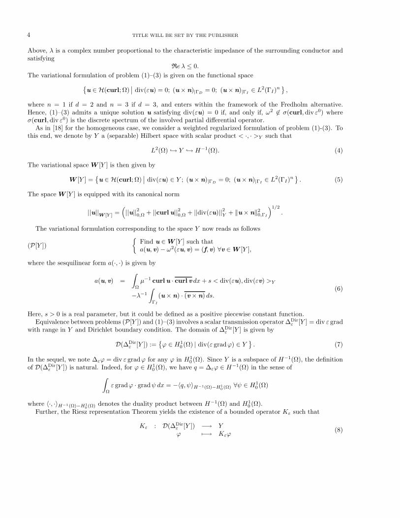
The variational formulation of problem (1)–(3) is given on the functional space

u ∈ H(curl; Ω)

∣∣ div(εu) = 0; (u× n)|ΓD= 0; (u× n)|ΓI

∈ L2(ΓI)n,

where n = 1 if d = 2 and n = 3 if d = 3, and enters within the framework of the Fredholm alternative.Hence, (1)–(3) admits a unique solution u satisfying div(εu) = 0 if, and only if, ω2 6∈ σ(curl, div ε0) whereσ(curl, div ε0) is the discrete spectrum of the involved partial differential operator.

As in [18] for the homogeneous case, we consider a weighted regularized formulation of problem (1)-(3). Tothis end, we denote by Y a (separable) Hilbert space with scalar product < ·, · >Y such that

L2(Ω) → Y → H−1(Ω). (4)

The variational space W [Y ] is then given by

W [Y ] =u ∈ H(curl; Ω)

∣∣ div(εu) ∈ Y ; (u× n)|ΓD= 0; (u× n)|ΓI

∈ L2(ΓI)n. (5)

The space W [Y ] is equipped with its canonical norm

||u||W [Y ] =

(||u||20,Ω + ||curl u||20,Ω + ||div(εu)||2Y + ‖u× n‖2

0,ΓI

)1/2

.

The variational formulation corresponding to the space Y now reads as follows

(P [Y ])

Find u ∈ W [Y ] such thata(u, v) − ω2(εu, v) = (f, v) ∀v ∈ W [Y ],

where the sesquilinear form a(·, ·) is given by

a(u, v) =

∫

Ω

µ−1 curlu · curl v dx+ s < div(εu), div(εv) >Y

−λ−1

∫

ΓI

(u× n) · (v× n) ds.(6)

Here, s > 0 is a real parameter, but it could be defined as a positive piecewise constant function.Equivalence between problems (P [Y ]) and (1)–(3) involves a scalar transmission operator ∆Dir

ε [Y ] = div ε gradwith range in Y and Dirichlet boundary condition. The domain of ∆Dir

ε [Y ] is given by

D(∆Dirε [Y ]) :=

ϕ ∈ H1

0 (Ω) | div(ε gradϕ) ∈ Y. (7)

In the sequel, we note ∆εϕ = div ε gradϕ for any ϕ in H10 (Ω). Since Y is a subspace of H−1(Ω), the definition

of D(∆Dirε [Y ]) is natural. Indeed, for ϕ ∈ H1

0 (Ω), we have q = ∆εϕ ∈ H−1(Ω) in the sense of

∫

Ω

ε gradϕ · gradψ dx = −〈q, ψ〉H−1(Ω)−H1

0(Ω) ∀ψ ∈ H1

0 (Ω)

where 〈·, ·〉H−1(Ω)−H1

0(Ω) denotes the duality product between H−1(Ω) and H1

0 (Ω).Further, the Riesz representation Theorem yields the existence of a bounded operator Kε such that

Kε : D(∆Dirε [Y ]) −→ Yϕ 7−→ Kεϕ

(8)


where Kεϕ is the unique element in Y such that

< p,Kεϕ >Y = 〈p, ϕ〉H−1(Ω)−H1

0(Ω) ∀p ∈ Y.

We are now able to state the following equivalence result:

Theorem 2.1. Let f ∈ L2(Ω)d be divergence-free, div f = 0 in Ω and assume that ω 6= 0. Let u be a solution to

(P [Y ]). If the range of the operator ∆Dirε [Y ] + ω2

s Kε is dense in Y , then div(εu) = 0 in Ω and u is a solutionto (1–3).

The idea of the proof is the same as in [18] and is omitted here. It is obvious that any solution of (1)–(3)satisfies (P [Y ]). Under the condition of Theorem 2.1, problem (P [Y ]) has thus a unique solution wheneverω2 6∈ σ(curl, div ε0).

Remark 2.2. (1) The result of Theorem 2.1 carries over to the case ω = 0, since the range of ∆Dirε [Y ] is

the whole space Y provided that Y ⊂ H−1(Ω).(2) If the imbedding of Y in H−1(Ω) is compact, we can prove in a similar way as in [18], that W [Y ] is

compactly imbedded in L2(Ω)d (see also [21] for the case Y = L2(Ω)). The sesquilinear form a(·, ·) isthus coercive on the space W [Y ].

(3) As in [18], the space Y will be defined later on as a weighted L2-space. Therefore, the range of

∆Dirε [Y ]+ ω2

s Kε will be dense in Y if and only if ω2

s does not belong to the spectrum of a scalar positive

self-adjoint operator with compact inverse (see [18] for details). Hence, taking s such that ω2

s is smallerthan the smallest eigenvalue of this operator guarantees the equivalence between (P [Y ]) and the originalproblem.

Let us finally introduce the following spaces of piecewise regular functions

PHs(Ω;P) =ϕ ∈ L2(Ω) | ϕj ∈ Hs(Ωj), j = 1, . . . , J

, (9)

where ϕj denotes the restriction of ϕ to Ωj . We denote by PH s(Ω;P) the corresponding spaces of vector fields.

The remainder of this first part is to show that the space W [Y ] ∩ PH 1(Ω;P) is dense in W [Y ] for anappropriated choice of the space Y . As mentioned before, the main application is the possibility to approximatethe problem (P [Y ]) by means of nodal finite elements.

2.2. Scalar potentials

With regard to the density results that we address here, we prove in this subsection that it is sufficient todeal with the question in terms of scalar potentials only. We introduce the following functional space

H [Y ] =ϕ ∈ H1(Ω)

∣∣ ∆εϕ ∈ Y ; ϕ|ΓD= 0; ϕ|ΓI

∈ H1(ΓI); l(ϕ) = 0

(10)

where l is a continuous linear form on H1(ΓI) such that l(1) 6= 0. The space H [Y ] is equipped with its canonicalnorm

||ϕ||H[Y ] =

(||ϕ||21,Ω + ||∆εϕ||2Y +

∑

F∈FI

||ϕ||21,F

)1/2

. (11)

It is a space of scalar potentials associated with the space of vector fields W [Y ] in the sense that

gradH [Y ] ⊂ W [Y ].

Notice that in general, scalar potentials are uniquely determined up to an additive constant. Here, the linearform l is introduced in the space H [Y ] in order to fix this constant. In the case where ∂Ω is not connected, onelinear form for each connected component including a part from ΓI should be included in H [Y ].


The first step will be the decomposition of the elements of W [Y ] into a (piecewise) regular part and a singularpart, the singular part deriving from a scalar potential.

Theorem 2.3. Let u ∈ W [Y ]. There is a scalar function ϕ ∈ H [Y ] and a piecewise regular vector fielduR ∈ W [Y ] ∩ PH 1(Ω;P) such that

u = uR + gradϕ. (12)

Further, there is a constant c > 0 independent from u such that

||uR||PH1(Ω;P) + ||ϕ||H[Y ] ≤ c ||u||W [Y ] . (13)

Proof. Let u ∈ W [Y ]. Since div(εu) ∈ Y ⊂ H−1(Ω), there is a unique function χ ∈ H10 (Ω) such that

∆εχ = div(εu). Thus, the vector field v = u− gradχ satisfies

∣∣∣∣∣∣∣∣

curl v = curlu in Ωdiv(εv) = 0 in Ωv× n = 0 on ΓD

v× n = u× n on ΓI .

Hence, v belongs to the standard regularization space W[L2(Ω)]. From [29] (Theorem 3.2), we deduce theexistence of a regular vector potential uR ∈ W[L2(Ω)] ∩ PH 1(Ω;P) satisfying

∣∣∣∣∣∣

curluR = curl v in Ωdiv(εuR) ∈ L2(Ω)uR × n = 0 on ∂Ω

as well as the estimate

||uR||PH1(Ω;P) + ||div(εuR)||0,Ω ≤ c ||curl v||0,Ω . (14)

Since curl(u− uR) = curl(v− uR) = 0 in Ω, there is a unique scalar potential ϕ ∈ H1(Ω) such that

gradϕ = u− uR in Ω andl(ϕ) = 0.

We obviously have ∆εϕ ∈ Y . Moreover, ϕ|ΓIbelongs to H1(ΓI) since

gradT ϕ|F = gradϕ|F × n = u|F × n ∈ L2(F )n ∀F ⊂ ΓI .

This shows that ϕ belongs to H [Y ].We prove in Lemma 2.4 below that

||ϕ||H[Y ] ≤ c

(||∆εϕ||2Y +

∑

F∈FI

||gradT ϕ||20,F

)1/2

∀ϕ ∈ H [Y ].

The estimate of ||∆εϕ||Y follows from the continuous imbedding of L2(Ω) in the vector space Y and (14), takinginto account that curl v = curlu:

||∆εϕ||Y ≤ ||div(εu)||Y + c ||div(εuR)||0,Ω

≤ c(||div(εu)||Y + ||curlu||0,Ω)

≤ c ||u||W [Y ]


whereas the second term is equal to ∑

F∈FI

||u× n||20,F

according to the definition of ϕ. This proves (13).

In the proof of Theorem 2.3, we made use of the following equivalence result between norms:

Lemma 2.4. Let Y be such that (4) holds. The application

|·|H[Y ] : H [Y ] −→ R+

ϕ 7−→(||∆εϕ||2Y +

∑

F∈FI

||gradT ϕ||20,F

)1/2

defines a norm on H [Y ] equivalent to the canonical norm ||·||H[Y ].

Proof. It is obvious that |·|H[Y ] defines a semi-norm on H [Y ]. Now, let ϕ ∈ H [Y ] be such that |ϕ|H[Y ] = 0.

Hence, ∆εϕ = 0 on Ω which yields ϕ = 0 on Ω if ΓD 6= ∅. If ΓD = ∅, we have gradT ϕ = 0 on all exterior faces.Hence, ϕ|∂Ω is a constant and this constant must be 0 since l(ϕ) = 0 and l(1) 6= 0.

We next prove equivalence between |·|H[Y ] and the canonical norm. Let ϕ ∈ H [Y ]. There is a unique function

r ∈ H1(Ω) such that∆εr = 0 in Ωr = ϕ on ∂Ω.

It follows from classical results in variational theory and the continuous imbedding H1(ΓI) → H1/2(ΓI) that

||r||1,Ω ≤ c‖ϕ‖1/2,∂Ω ≤ c

( ∑

F∈FI

||ϕ||21,F

)1/2

. (15)

Next, let ϕ = ϕ− r. The function ϕ is the variational solution in H10 (Ω) to the following Dirichlet problem with

data in Y :∆εϕ = ∆εϕ in Ωϕ = 0 on ∂Ω

.

We deduce from Poincare’s inequality and the definition of the parameter ε that

||ϕ||21,Ω ≤ c

∫

Ω

ε| grad ϕ|2 dx

= −c〈∆εϕ, ϕ〉H−1(Ω)−H1

0(Ω)

≤ c‖∆εϕ‖−1,Ω ||ϕ||1,Ω ,

and thus

||ϕ||1,Ω ≤ c ||∆εϕ||Y (16)

since the imbedding Y → H−1(Ω) is continuous. Finally, we deduce from (15) and (16) that

||ϕ||1,Ω ≤ c

(||∆εϕ||2Y +

∑

F∈FI

||ϕ||21,F

)1/2

and the result follows from the equivalence between the H1-norm and the seminorm∑

F∈FI| · |1,F in the space

w ∈ H1(ΓI) | l(w) = 0.


Note that the above decomposition (12) is not unique. For instance take ψ ∈ D(Ωj) for a fixed j ∈ 1, · · · , Jand let u′

R = uR + ||u||W [Y ] gradψ and ϕ′ = ϕ− ||u||

W [Y ] ψ. Obviously,

u = u′R + gradϕ′

and u′R and ϕ′ satisfy (13).

Nevertheless, due to the decomposition (12) and estimate (13), we are able to define a linear continuousapplication Φ : W [Y ] −→ H [Y ] which maps any vector field u ∈ W [Y ] on the corresponding scalar potentialϕ ∈ H [Y ] in the sense that

u− grad(Φ(u)) ∈ W [Y ] ∩ PH 1(Ω;P) and (17)

Φ(gradϕ) = ϕ ∀ϕ ∈ H [Y ]. (18)

Since gradH [Y ] ⊂ W [Y ], Φ is well defined and onto. Moreover, Φ maps regular vector fields on regular scalarpotentials, i.e.

Φ(W [Y ] ∩ PH 1(Ω;P)

)⊂ H [Y ] ∩ PH2(Ω;P). (19)

Indeed, let u ∈ W [Y ] ∩ PH 1(Ω;P). Due to (17), we have grad(Φ(u)) ∈ PH 1(Ω;P) which implies that

Φ(u) = ϕ ∈ PH2(Ω;P).

We are now able to state the main result of this subsection:

Theorem 2.5. The space of vector fields W [Y ]∩PH 1(Ω;P) is dense in W [Y ] if, and only if, the correspondingspace of scalar potentials H [Y ] ∩ PH2(Ω;P) is dense in H [Y ].

Proof. The proof of Theorem 2.5 follows directly from the definition and the properties of the application Φ.We refer to [29] (Proof of Theorem 3.1) for details.

2.3. Two-dimensional results

In this subsection, we prove the density result in the case of a polygon for an appropriate choice of the spaceY . We further state some preliminary results which will be helpful for the edge singularities in three dimensions.In this subsection, Ω is a fixed polygon of the plane with the assumptions of §2.1.

Let us start with the definition of the space Y . For α ∈] − 1, 1[, we denote

Y =g ∈ H−1(Ω)

∣∣ wαg ∈ L2(Ω), (20)

where the weight function w is assumed to be positive on Ω. There are several possibilities to define the functionw (see [18]). Roughly speaking, w will be chosen to be equivalent to the distance function to the set of verticesof the subdomains. The space Y is a Hilbert space equipped with the scalar product

< f, g >Y =

∫

Ω

w2α(x)f(x)g(x) dx

In order to provide a rigorous definition of the weight function w, we introduce the following notations. LetS be the set of vertices of at least one Ωj . The set of exterior vertices will be denoted by Sext,

Sext = S ∈ S | S ∈ ∂Ω .

This set is split into two subsets, namely,

SD = Sext∩

ΓD

SI = Sext \ SD.


The set of interior vertices is given by Sint = S \ Sext.

Definition 2.6 (Weight function in two dimensions). Let Ω ⊂ R2 be a polygon. For any vertex S ∈ S, let(rS , θS) denote the local polar coordinates with respect to S. The weight function w is defined by

w(x) =∏

S∈S0

rS (21)

where S0 is a subset of S.

This definition is similar to the one of simplified weights in [18]. Notice that w(x) is equivalent to the distancefunction d(x) = dist(x,S). Moreover, in a sufficiently small neigbourhood VS of the vertex S containing noother vertex of Ω, the weight function is equivalent to rS if the weight is ”active”, whereas w(x) ≈ 1 far awayfrom the vertices. Let us now introduce

L2α(Ω) =

g ∈ H−1(Ω)

∣∣∣∣∣

( ∏

S∈S0

rS

)α

g ∈ L2(Ω)

.

The following result shows that L2α(Ω) is an admissible choice for the space Y :

Proposition 2.7. Let Y = L2α(Ω). Then (4) does hold for any α ∈ [0, 1[.

Proof. Since α ≥ 0 and w is continuous on Ω, the imbedding L2(Ω) → L2α(Ω) is obvious.

On the other hand, we deduce from a classic Hardy inequality (see for instance [33], Lemma 4.1 p. 38) that

H1(Ω) → L2−α(Ω)

for all α ∈ [0, 1[, if one recalls that the weight function w is equivalent to the distance function near the verticesand equivalent to 1 anywhere else.

The result of the Proposition follows by duality since (L2−α(Ω))′ = L2

α(Ω).

From now on, let Y be as in Proposition 2.7. For ξ ∈ R, we introduce the space of dual singularities Nε,ξ[Y ]defined as the orthogonal in Y of (∆ε − εξ2I)(H [Y ] ∩ PH2(Ω;P)) with respect to the scalar product of Y . Inother words, an element g ∈ Y belongs to Nε,ξ[Y ] if, and only if,

< g, (∆ε − εξ2I)ϕ >Y = 0 ∀ϕ ∈ H [Y ] ∩ PH2(Ω;P). (22)

We next recall the space of standard dual singularities Nε,Dir,ξ defined as follows: g ∈ Nε,Dir,ξ if, and only if,g ∈ L2(Ω) and ∫

Ω

g(∆ε − εξ2I)ϕdx = 0 ∀ϕ ∈ D(∆Dirε [L2(Ω)]) ∩ PH2(Ω;P) (23)

where D(∆Dirε [L2(Ω)]) is defined in analogy with (7). Taking into account the definition of the scalar product

< ·, · >Y , we are now able to state the following link between Nε,ξ[Y ] and Nε,Dir,ξ:

Proposition 2.8. Let ξ ∈ R. For any g ∈ Nε,ξ[Y ], the function gα defined by

gα = w2αg

belongs to the space of standard dual singularities, Nε,Dir,ξ.

Proof. (1) Let g ∈ Nε,ξ[Y ]. Since g belongs to Y = L2α(Ω), the function wαg belongs to L2(Ω). The

definition of the weight function w then guarantees that gα = w2αg ∈ L2(Ω).


(2) In order to prove that gα satisfies the orthogonality relation (23), let ϕ ∈ D(∆Dirε [L2(Ω)])∩PH2(Ω;P).

Then, ϕ also belongs to H [Y ] ∩ PH2(Ω;P), since L2(Ω) ⊂ L2α(Ω) and ϕ|∂Ω = 0. Hence

∫

Ω

gα(∆ε − εξ2I)ϕdx =< g, (∆ε − εξ2I)ϕ >Y = 0

which proves (23).

In view of the forthcoming Theorem 2.10, we need to recall the singularities of the transmission probleminvolving the operator ∆ε with domain D(∆Dir

ε [L2(Ω)]). (see [28, 34, 35] for details).For S ∈ Sext, let Λε,S be the set of positive singular exponents of the operator ∆Dir

ε [L2(Ω)] that we nowdescribe shortly. Without loss of generality we may assume that the set of subdomains Ωj having S as vertex

is ΩjJS

j=1, for some positive integer JS . For j ∈ 1, · · · , JS let ωj be the interior opening of Ωj at S and setσ0 = 0 and σj = σj−1 + ωj. Then a real number λ belongs to Λε,S if, and only if, there exists a non trivial

solution φλ ∈ H1(]0, σJS[), φλ = (φλ,j)

JS

j=1, to

φ′′λ,j + λ2φλ,j = 0 in ]σj−1, σj [, j = 1, · · · , JS , (24)

φλ,1(0) = φλ,JS(σJS

) = 0, (25)

[φλ]σj−1= [εφ′λ]σj−1

= 0, j = 1, · · · , JS − 1, (26)

where (rS , θS) are the local polar coordinates with respect to S, the half-line θS = σj containing an edge of Ωj ,for j = 1, · · · , JS while the half-line θS = 0 contains an edge of Ω1 (see Fig. 1).

Ω

ΩΩ

1

23

θ=0

θ=σ

θ=σθ=σ

1

23

S

Figure 1. Subdomains having a common vertex (JS = 3).

Note that in the homogeneous case, i.e., εj = ε, for all j = 1, · · · , JS , the set Λε,S is equal to kπσJS

: k ∈N, k 6= 0 and is independent of ε. In the inhomogeneous case this set is not explicitly known but may beapproximated numerically (see e.g. [28, 34, 35]).

We proceed similarly for S ∈ Sint, replacing the Dirichlet boundary condition (25) by the transmissionconditions

φλ,1(0) = φλ,JS(2π), ε1φ

′λ,1(0) = εJS

φ′λ,JS(2π).

Let us notice that if S ∈ Sext then λ ∈ Λε,S is simple (see [35]). In other words, the solution φλ to (24)-(25)is unique up to a multiplicative factor. On the other hand, if S ∈ Sint, then λ ∈ Λε,S has a finite multiplicityand in that case λ is repeated in Λε,S according to its multiplicity.

The standard singularities of the operator ∆Dirε [L2(Ω)] at the vertex S ∈ S are

SS,λ = ηSrλφλ, for λ ∈ Λε,S , (27)

where ηS = ηS(r) is an appropriate cut-off function (ηS ≡ 1 in a neighbourhood of S and ηS ≡ 0 in aneighbourhood of the other vertices).


Next, we need to characterize the elements of the space Nε,Dir,ξ. To this end, we recall Proposition 2.8.of [29] (for any details, see [34] for the case ξ = 0 and [24] for ξ 6= 0). Let us begin with some classical Grisvardnotations. For ` = 1, 2, let H`−1/2(∂Ω) be the range of the trace mapping, starting from H`(Ω) ; for all faces

F ∈ Fext, the restrictions of those sets to F is denoted by H`−1/2(F ). Then, define H`−1/2(F ) as the set

of elements of H`−1/2(F ) whose continuation by zero to ∂Ω belongs to H`−1/2(∂Ω). Finally, let H1/2−`(F )

denote the dual space of H`−1/2(F ). In the same manner, one can introduce similar spaces for the interiorfaces, starting from interior domains.

Proposition 2.9. g ∈ Nε,Dir,ξ if, and only if, g ∈ L2(Ω) is solution to

(∆ − ξ2I)g = 0 in Ωj ∀j,g = 0 in H−1/2(F )∀F ∈ Fext.

[g] = 0 in H−1/2(F )∀F ∈ Fint,

[ε∂ng] = 0 in H−3/2(F )∀F ∈ Fint.

In order to give an appropriate basis of Nε,Dir,ξ, we set for any vertex S ∈ S and all λ ∈ Λε,S ,

gS,λ,ξ = ηSe−|ξ|rr−λφλ − vS,λ,ξ, (28)

where vS,λ,ξ ∈ H10 (Ω) is the unique variational solution to

(∆ε − εξ2I)vS,λ,ξ = (∆ε − εξ2I)(ηSe−|ξ|rr−λφλ), (29)

i.e., is the unique solution to

∫

Ω

ε(gradvS,λ,ξ · gradw + ξ2vS,λ,ξw) dx

= −∫

Ω

(∆ε − εξ2I)(ηSe−|ξ|rr−λφλ)w dx, ∀w ∈ H1

0 (Ω).

Notice that this problem is well defined since the right hand side of (29) belongs to Lq(Ω) with q < 21+λ (see

Lemma 4.4 and 4.5 of [27]).The function gS,λ,ξ belongs to Nε,Dir,ξ and satisfies (thanks to Green’s formula, see Proposition 2.5.5 of [24]))

∫

Ω

(∆ε − εξ2I)(ηT rµφµ)gS,λ,ξ dx = 2λδS,T δλ,µ. (30)

Furthermore, under the assumption1 6∈ Λε,S , ∀S ∈ S, (31)

the set gS,λ,ξλ∈Λε,S∩]0,1[,S∈S is a basis of Nε,Dir,ξ.The following Theorem provides an appropriate condition on the weight exponent α such that the density

result for the scalar potentials (and thus also for the corresponding space of vector fields) holds true:

Theorem 2.10. Let Y be as in Proposition 2.7. Let the subset S0 ⊂ S satisfy the following inclusion:

S ∈ SD ∪ Sint | Λε,S∩]0, 1[6= ∅ ∪ S ∈ SI | Λε,S∩]0, 1/2[6= ∅ ⊂ S0. (32)

Further, let α be such that

α > 1 − min

⋃

S∈SD∪Sint

(Λε,S∩]0, 1[) ∪⋃

S∈SI

(Λε,S∩]0, 1/2[)

(33)


Assume that (31) holds. Then H [Y ] ∩ PH2(Ω;P) is dense in H [Y ].

Proof. In order to prove the density result, we will characterize the elements of some complementary space O[Y ]that wedefine here. Let

H0[Y ] =ϕ ∈ H1(Ω)

∣∣ ∆εϕ ∈ Y ; ϕ|ΓD= 0; ϕ|F ∈ H1

0 (F ), ∀F ∈ FI

.

As in [29], we prove that H0[Y ] is continuously imbedded in H [Y ] if we choose the linear form l in the definitionof H [Y ] as follows:

l(ϕ) =∑

S∈SI

ϕ(S).

Now, let ξ ∈ R and let O[Y ] be the orthogonal complement of H0[Y ] ∩ PH2(Ω;P) for the inner product

(ϕ, ψ)ξ,Y = < (∆ε − εξ2I)ϕ, (∆ε − εξ2I)ψ >Y

+∑

F∈FI

(gradT ϕ, gradT ψ)0,F + ξ2(ϕ, ψ)0,F

.

ThenH [Y ] = H [Y ] ∩ PH2(Ω;P) ⊕O[Y ]

since the complementary space of H0[Y ] in H [Y ] is spanned by a finite number of functions that belong toH [Y ] ∩ PH2(Ω;P). Notice that arguments, similar to those of Lemma 2.4, allow one to show that the norm

‖ϕ‖ξ,Y = (ϕ,ϕ)1/2ξ,Y is equivalent to ||·||H[Y ] with equivalence constants that depend on ξ.

As in [29] (Proposition 4.3), we are able to prove that for any f ∈ O[Y ], there is a unique g ∈ Nε,ξ[Y ] with

(∆ε − εξ2I)f = g in Y, (34)

(∆T − ξ2I)f = −ε∂νgα in H−1(F ), ∀F ∈ FI , (35)

‖f‖ξ,Y ≤ c

(||g||Y +

∑

F∈FI

‖ε∂νgα‖−1,F

)(36)

where gα = w2αg is the standard dual singularity in Nε,Dir,ξ corresponding to g, according to Proposition 2.8.The function gα is thus uniquely represented as

gα =∑

S∈S

∑

λ∈Λε,S∩]0,1[

cλ,SgS,λ,ξ.

As in the proof of Theorem 4.4 in [29], condition (35) implies that

cλ,S = 0 ∀λ ∈ Λε,S ∩ [1/2, 1[, ∀S ∈ SI

since ∂νgS,λ,ξ ≈ rλ−1S near S.

Now, let λ ∈ Λε,S∩]0, 1[ for a vertex S ∈ SD ∪Sint or λ ∈ Λε,S∩]0, 1/2[ for S ∈ SI . Taking into account thatwαg belongs to L2(Ω), we deduce that w−αgS,λ,ξ ∈ L2(Ω) whenever cλ,S 6= 0. But

w−αgS,λ,ξ ≈ r−(α+λ)S Φλ,S(θS)

near S, and r−(α+λ)S Φλ,S belongs to L2(Ω) if, and only if, α+λ < 1 which is in contradiction with the assumption

on α. Therefore cλ,S = 0 for any λ which yields g = 0 in Ω.Finally, we deduce from (36) that f = 0 in Ω which completes the proof.


Remark 2.11. One could also consider general weights with an exponent that depends on the vertex S of S.Namely, one could replace wα by ∏

S∈S

rαS

S , (37)

with (αS)S∈S in ]0, 1]|S| such that

αS > 1 − min (Λε,S∩]0, 1[) if S ∈ SD ∪ Sint ;αS > 1 − min (Λε,S∩]0, 1/2[) if S ∈ SI .

(38)

2.4. Density results in three-dimensional domains

In this subsection we investigate a suitable condition on the weight exponent α in order to obtain the densityresult in the case of a three dimensional Lipschitz-polyhedron.

In order to define the weight function w, we introduce the following notations which describe the domain Ωnear the geometric singularities.

Let S (resp. E) be the set of vertices (resp. edges) of at least one Ωj . The subscripts ext and int will denoteexterior and interior vertices or edges as before, and the set Sext (resp. Eext) admits the following splitting,according to the different boundary conditions:

SD = Sext∩

ΓD, SI = Sext \ SD,

ED = Eext∩

ΓD, EI = Eext \ ED.

For a vertex S ∈ S, let ΓS be the polyhedral cone which coincides with Ω near S and let GS be the intersectionof ΓS with the unit sphere. We shall use local spherical coordinates (rS , σS) centered at S. To each edge eadjacent to the vertex S, corresponds a corner of GS denoted by Se. A neighbourhood of the point Se may thusbe mapped on an infinite plane sector which can be written in polar coordinates as

CS,e = (ϑS,e, ϕS,e) | ϑS,e > 0, 0 < ϕS,e < ωS,e .

Next, let e ∈ E be an (exterior or interior) edge with opening angle ωe ∈ ]0, 2π] (ωe = 2π if, and only if,e ∈ Eint). Without loss of generality, we may assume that e is supported by the z-axis and we denote (re, θe, z)the corresponding cylindrical coordinates. In particular, we have

re(x) = dist(x, e) ∀x ∈ Ω.

Let us fix Re > 0 and he > 0 and introduce the two-dimensional domain

Ωe := (re cos θe, re sin θe) | 0 < re < Re, 0 < θe < ωe

such that the dihedral coneDe = Ωe × R (39)

coincides with Ω for any z ∈]−he, he[ and does contain no other edge nor any vertex of Ω. To each Ωj containinge, there corresponds a unique set Ωe,j ⊂ Ωe. Therefore the partition P induces a natural partition Pe of Ωe

(and thus De) for which ε and µ are piecewise constant and depend only on θ. Namely, we take

εe,j = εj on Ωe,j × R,µe,j = µj on Ωe,j × R.

We finally denote Γe,0 (resp. Γe,ω) the edges of Ωe and Fe,0 = Γe,0 × R (resp. Fe,ω) the corresponding exteriorfaces of De containing e.


If we denote by dS(x) (resp. dE) the distance function to the set S (resp. E), i. e.

dS(x) = dist(x,S) and dE(x) = dist(x, E),

we clearly havedS ≈ rS

in any sufficiently small neighbourhood VS of the vertex S, and

dE ≈ re

in Ωe×] − he, he[ for sufficiently small numbers Re and he.In order to define the weight function, we need to introduce another distance function ρe taking into account

the edge/vertex interaction. Let e ∈ E be the segment between the two vertices S and S′. Then we define ρe by

re = ρerSrS′ . (40)

In a sufficiently small neighbourhood of the vertex S, the function ρe is equivalent to the angular distance ϑS,e

near the edge e, whileρe ≈ dE far from S.

The definition of the weight function then reads as follows (see the definition of global weights in [18]):

Definition 2.12 (Weight function in three dimensions). Let Ω ⊂ R3 be a Lipschitz-polyhedron. The weightfunction w is defined by

w(x) =

( ∏

S∈S0

rS

)(∏

e∈E0

ρe

)(41)

where S0 ⊂ S and E0 ⊂ E satisfy the following compatibility condition: if e ∈ E0 is an edge with end points Sand S′, then S ∈ S0 and S′ ∈ S0.

It has been proven in [18] that an equivalent definition is

w(x) = dist (x,S0 ∪ E0) .

This corresponds to the simple weights of Costabel-Dauge, where the set S0 ∪ E0 is a so-called wire basket, inthe spirit of [36].

As in two dimensions, we have the

Proposition 2.13. Let Y = L2α(Ω) with a weight function as in Definition 2.12. Then (4) does hold for any

α ∈ [0, 1[.

Proof. As in two dimensions, the first imbedding L2(Ω) → L2α(Ω) is obvious. For the second imbedding, we

proceed by duality, proving thatH1

0 (Ω) → L2−α(Ω).

Near an edge, this follows as in two dimensions from the classical Hardy inequality. Near the vertices, we mayuse Proposition 5.1. in [30] since the definition of weights therein is equivalent to Definition 2.12.

We next describe the vertex and edge singularities of the operator ∆ε with Dirichlet boundary condition,i. e. with domain D(∆Dir

ε [L2(Ω)]). The set Λε,S of positive vertex singular exponents is related to the spectrumof the nonnegative Laplace-Beltrami operator Lε,S . More precisely, it is the Friedrichs extension of the triple(Hε,S , VS , aε,S), where Hε,S = L2(GS) with the inner product

(ψ, φ)ε =

∫

GS

εψφdσ,


the space VS being equal to H10 (GS) if S ∈ Sext, and VS = H1(GS) if S ∈ Sint, and finally

aε,S : VS × VS → R : (ψ, φ) →∫

GS

ε gradT ψ · gradT φdσ.

The operator Lε,S is a nonnegative selfadjoint operator on Hε,S with a compact inverse. Let 0 ≤ ν1 ≤ ν2 · · ·be its eigenvalues repeated according to their multiplicity. We further denote by φj ∈ VS the eigenfunctionassociated with νj . According to [19], we have

Λε,S \ N =

−1

2+

√νj +

1

4| j ≥ 1

\ N

and 0 6∈ Λε,S . For λ ∈ Λε,S , we will denote by φλ the eigenfunction φj for which λ = − 12 +

√νj + 1

4 (with the

above convention φλ is uniquely defined). As in two dimensions, for S ∈ S the standard singularities of theoperator ∆ε at the vertex S ∈ S are given by (27).

As the edge e of Ω corresponds to a vertex Se of Ωe, the set Λε,e of edge singular exponents is given by

Λε,e = Λε,Se,

where Λε,Seis the set of corner singularities defined in §2.3 (here at Se in Ωe). In other words, the edge

singularities are induced by the corner singularities at Se in Ωe.The goal of this subsection is to show the following density result:

Theorem 2.14. Let E0 ⊂ E such that

e ∈ ED ∪ Eint | Λε,e∩]0, 1[6= ∅ ∪ e ∈ EI | Λε,e∩]0, 1/2[6= ∅ ⊂ E0. (42)

Let S0 ⊂ S such thatS ∈ SD ∪ Sint | Λε,S∩]0, 1/2[6= ∅ ⊂ S0 (43)

and assume that E0 and S0 satisfy the compatibility condition of Definition 2.12. Assume further that

1/2 6∈ Λε,S , ∀S ∈ S and 1 6∈ Λε,e, ∀e ∈ E . (44)

Let Y = L2α(Ω) where α ∈ [0, 1[ satisfies

α > 1 − min (Λε,e∩]0, 1[) ∀e ∈ E0 ∩ (ED ∪ Eint) (45)

α > 1 − min (Λε,e∩]0, 1/2[) ∀e ∈ E0 ∩ EI (46)

α > 1/2 − min (Λε,S∩]0, 1/2[) ∀S ∈ S0 ∩ (SD ∪ Sint) (47)

Then the space H [Y ] ∩ PH2(Ω;P) is dense in H [Y ].

The arguments of the proof of Theorem 2.14 are similar to those in [29] (Theorem 5.1). In a first step, wereduce the density problem from H [Y ] to that of the closed subspace

H0[Y ] =ϕ ∈ H

∣∣ ϕ|F ∈ H10 (F ) ∀F ∈ FI

which makes sense if we define the linear form l involved in the definition of H [Y ] by

l(ϕ) =∑

e∈EI

∫

e

ϕ(s) ds


(we recall that this definition is meaningful since the trace on a face F ∈ FI of any element of H [Y ] belongs toH1(F ) → L1(e)). As in [29] (Proposition 5.3) we have the

Proposition 2.15. If H0[Y ] ∩ PH2(Ω;P) is dense in H0[Y ], then H [Y ] ∩ PH2(Ω;P) is dense in H [Y ].

As in two dimensions, the proof of Theorem 2.14 relies on a careful analysis of the dual singularities associatedwith the weighted space Y , that are defined by:

Nε[Y ] =g ∈ Y

∣∣ < g,∆εϕ >Y = 0 ∀ϕ ∈ H0[Y ] ∩ PH2(Ω;P). (48)

The standard dual singularities are given by

Nε =g ∈ L2(Ω)

∣∣ (g,∆εϕ) = 0 ∀ϕ ∈ D(∆Dirε [L2(Ω)]) ∩ PH2(Ω;P)

. (49)

From [29] (Proposition 5.5 and Lemma 5.6) we recall the following characterization of the elements of Nε:

Proposition 2.16. Let g ∈ Nε. Then g is solution to

∆g = 0 in Ωj ∀j, (50)

g = 0 in H−1/2(F )∀F ∈ Fext. (51)

[g] = 0 in H−1/2(F )∀F ∈ Fint, (52)

[ε∂ng] = 0 in H−3/2(F )∀F ∈ Fint. (53)

Moreover, g belongs to⋃

j C∞(Ωj \ V) where V is any neighbourhood of the geometric singularities of Ω (edges

and corners of at least one Ωj).

Proof of Theorem 2.14. Let O[Y ] ⊂ H0[Y ] be the orthogonal space of H0[Y ] ∩ PH2(Ω;P) and take f ∈ O[Y ],i. e.

< ∆εf,∆εϕ >Y +∑

F∈FI

(gradT f, gradT ϕ)0,F = 0 ∀ϕ ∈ H0[Y ] ∩ PH2(Ω;P).

Now, let g = ∆εf . Since L2(Ω) → Y , we get

< g,∆εϕ >Y = 0 ∀ϕ ∈ D(∆Dirε [L2(Ω)]) ∩ PH2(Ω;P).

As in Proposition 2.8, the function gα = w2αg thus belongs to Nε and satisfies

w−αgα ∈ L2(Ω).

Moreover, applying the arguments of the proof of Proposition 5.7 in [29], we show that

−ε∂ngα = ∆T f ∈ H−1(F ) ∀F ∈ FI .

According to Proposition 2.20 below, these supplementary regularity results guarantee that gα belongs toH1(Ω). On the other hand, gα is a solution to the homogeneous problem ∆εgα = 0 in Ω and gα = 0 on ∂Ω (seeProposition 2.16). This implies that gα vanishes in Ω and so does g = w−2αgα.

Finally, f ∈ H0[Y ] is the variational solution to the homogenous problem

∆εf = 0 in Ω,f = 0 on ΓD,∆T f = 0 on ΓI .

Hence, f = 0 in Ω which proves the density result.


According to the proof of Theorem 2.14, we shall consider in the sequel a function gα ∈ Nε satisfying

w−αgα ∈ L2(Ω) (54)

andε∂ngα ∈ H−1(F ) ∀F ∈ FI . (55)

In order to describe its behaviour near an edge e, we introduce a cut-off function ϕe with respect to e whichis given by

ϕe(re, θe, z) = ψ(re)χ(z) (56)

with ψ ∈ C∞([0,∞[), ψ ≡ 1 if 0 ≤ r ≤ r0/3, ψ ≡ 0 if r ≥ 2r0/3 and χ ∈ D(] − h, h[), χ ≡ 1 on [−h/2, h/2].Thus ϕe ≡ 1 in the neigbourhood of an interior part of e, and ϕe vanishes near any other geometric singularityof Ω.

In Lemma 2.17 below we prove that the elements of Nε coincide with those of the corresponding space onthe infinite cone De modulo a function of class H1. To this end, let us introduce the space

Nε(De) =ϕ ∈ L2(De)

∣∣ (ϕ,∆εψ)De= 0 ∀ψ ∈ PH2(De;Pe) ∩ (H0[Y ] ∩H1

0 (De)).

For any function ϕ of L2(Ωe×] − h, h[), ϕ denotes its extension by zero on De. We now prove the

Lemma 2.17. Let gα ∈ Nε with 0 ≤ α < 1. Let ϕe be as in (56). There is a unique function g∗ ∈ H10 (De)

such thatg0,α := g∗ − ϕeg ∈ Nε(De). (57)

Moreover, if gα satisfies (54) and (55), then

d−αe g0,α ∈ L2(De) and (58)

ε∂g0,α ∈ H−1(Fe,0) if e ∈ EI (59)

where de(x) = dist(x, e) denotes the distance function with respect to the edge e.

Proof. (57) and (59) have been proved in Lemma 5.8 in [29].Now, suppose that gα ∈ Nε satisfies in addition (54). We deduce from Hardy’s inequality that g∗/de belongs

to L2(De) since g∗ ∈ H10 (Ω) and de = re in De. Hence, d−α

e g∗ ∈ L2(De) for all α ∈ [0, 1[ since d−αe < d−1

e neare.

In order to prove that d−αe ϕeg ∈ L2(De), we notice that

d−αe ϕegα ≈ ϕew

−αgα on Ωe×] − h, h[

whereas d−αe ϕegα = 0 anywhere else. We thus conclude with the help of condition (54).

The main tool to investigate edge singularities is the partial Fourier transform in the edge variable z: for agiven function v ∈ L2(De), we denote

Fv(x′, ξ) = v(x′, ξ) =1√2π

∫

R

v(x′, z)e−iξzdz.

Then we have the following

Lemma 2.18. Let g ∈ Nε(De). Then g(·, ξ) ∈ Nε,Dir,ξ for almost every ξ ∈ R (here Nε,Dir,ξ, defined in §2.3,is based on Ωe instead of Ω). If in addition, g satisfies (58) and (59), then

r−αe g(·, ξ) ∈ L2(Ωe) and (60)

ε∂ng ∈ H−1(Γe,0) if e ∈ EI (61)

for almost every ξ ∈ R.


Proof. The first part has been proved in Lemma 5.9 in [29]. We deduce from Lemma 2.17 that d−αe g ∈ L2(De).

(60) then follows since de(x) = re does not depend on z and thus

d−αe g(·, ξ) = r−αg.

In the same way, we get (61) since the normal vector n is invariant in z.

The following Proposition yields a condition on α in order to get H1-regularity of gα near the edges:

Proposition 2.19. Let 0 ≤ α < 1. Consider an edge e ∈ E and assume that 1 6= Λε,e. Let gα ∈ Nε satisfy(54) and (55). Assume that α > 1 − min (Λε,e∩]0, 1[) if e ∈ (ED ∪ Eint) ∩ E0, and α > 1 − min (Λε,e∩]0, 1/2[) ife ∈ EI ∩ E0. Then ϕegα ∈ H1(Ω) where ϕe is a cut-off function defined as in (56).

Proof. Lemma 2.17 implies that there exists g0,α ∈ Nε(De) satisfying (58) and (59) such that g0,α + ϕegα ∈H1

0 (De). Under the given assumptions on α, we then deduce from Lemma 2.18 and Section 2.3 that

g0,α(·, ξ) = 0

for almost every ξ ∈ R which yieldsg0,α = 0 on De.

In other words,ϕegα ∈ H1

0 (De)

which completes the proof.

We are now able to prove the following global regularity result:

Proposition 2.20. Let 0 ≤ α < 1. Let gα ∈ Nε satisfy (54) and (55). Assume further conditions (44), (45),(46) and (47) to be true. Then gα ∈ H1(Ω).

Proof. Under the given assumptions, we already know that gα exhibits the H1-regularity away from the corners.As the function gα belongs to Nε (and thus to L2(Ω)), one infers the following decomposition near a vertexS ∈ S

gα(rS , σS) =∑

l∈N

gl(rS)φl(σS),

where φl denotes the orthonormalized eigenfunction corresponding to the (nonnegative) eigenvalues νl of theLaplace-Beltrami operator Le,S on GS (for the inner product (·, ·)ε). For l ∈ N, the coefficient gl is given by

gl(rS) = alrλl

S + blrµl

S

where

λl = −1

2+

√νl +

1

4and µl = −1

2−√νl +

1

4(see [23] for details). Notice that λl ≥ 0 and µl ≤ −1 since νl ≥ 0 for all l ∈ N.

As the function gα belongs to L2(Ω), we notice that bl = 0 for any l ∈ N such that µl ≤ −3/2.Now, let S ∈ SI . Since gα ∈ Nε, is satisfies a Dirichlet boundary condition on ∂Ω (see Proposition 2.16).

Hence, all eigenvalues νl are positive which implies µl 6= −1. Moreover, there is at least one face F ∈ FI suchthat S is a vertex of F . Taking into account that ε∂ngα ∈ H−1(F ) thanks to (55), we deduce as in [29] thatbl = 0 for all µl ∈] − 3/2,−1[. Therefore

gα(rS , σS) =∑

l∈N

alrλl

S φl(σS)

and gα belongs to H1 in the cone ΓS(R′) with basis GS and height R′ for any R′ < RS .


Next, take a vertex S ∈ SD. Again, µl < −1 thanks to the Dirichlet boundary condition. If Λε,S∩]0, 1/2[= ∅,we have µl < −3/2 and hence

gα(rS , σS) =∑

l∈N

alrλl

S φl(σS).

We thus conclude as before.Now, let S ∈ S0 such that Λε,S∩]0, 1/2[6= ∅. Taking into account that gα satisfies (54), we must have

alr−α+λl

S φl(σS) ∈ L2(Ω) (62)

and

blr−(α+λl+1)S φl(σS) ∈ L2(Ω) (63)

for any λl where we used that λl + µl = −1. (62) is always satisfied since λl ≥ 0 and 0 ≤ α < 1. Thanks to(47), α > 1

2 − λl for any λl ∈ Λε,S∩]0, 1/2[. Hence, property (63) is satisfied if and only if bl = 0 for all l ∈ N

because α+ λl + 1 > 32 .

Again, we conclude that gα ∈ H1(ΓS(R′)) for any R′ < R.Finally, let S ∈ Sint. Now, ν1 = 0 is an eigenvalue of the operator Le,S and φ1 = cε denotes the associated

(constant) eigenfunction. gα thus splits as follows,

gα = g1(rS)φ1(σS) +∑

l≥2

gl(rS)φl(σS). (64)

But gα belongs to Nε and thus ∫

Ω

gα∆εηS dx = 0,

where ηS = ηS(rS) is any regular cut-off function such that ηS ≡ 1 near the vertex S and ηS ≡ 0 near the othervertices. Indeed, such a function belongs to D(∆Dir

ε [L2(Ω)])∩PH2(Ω;P) and is admissible in the orthogonalityrelation that defines Nε (see (49)). As in [24], we prove that

∫

Ω

gα∆εηS dx = cε

∫ ∞

0

g1(rS)(η′′S(rS) +2

rSη′S(rS))r2S dr

since ∫

GS

εφl(σS) dσ = 0

for all l ≥ 2. It follows that the integral of the second term in (64) vanishes. But g1(rS) = a1 + b1r−1S and an

elementary calculation shows that

∫ ∞

0

g1(rS)(η′′S(rS) +2

rSη′S(rs))r

2S dr = −b1

which yields b1 = 0. We then conclude as in the case S ∈ SD that gα ∈ H1(ΓS(R′)) for any R′ < R.

3. Discretization and convergence

In this section, we describe the discretization of problem (P [Y ]) by means of conforming nodal finite elementsof order k, and we prove convergence of the numerical method.


3.1. Discretization

Consider a family of simplicial meshes (Th)h of Ω, with h = maxTl∈Thhl, which is compatible with the

partition P (in the sense that all simplices lie in exactly one Ωj , j = 1, . . . , J). With Th, we associate the spaceof vector finite elements

X h =vh ∈ PH 1(Ω;P)

∣∣ vh|Tl∈ Pk(Tl)

d, ∀Tl ∈ Th

(65)

where d = 2 or d = 3. Let MI1,...,nbn be the set of nodes of the mesh Th. The discretization space V h is the

subspace of X h defined by V h = X h ∩ W [Y ] ⊂ PH 1(Ω;P) ∩ W [Y ], that is

V h = vh ∈ X h | ”[vh × n](MI) = 0”; ”[εvh · n](MI) = 0” ∀MI ∈ Fint ”(vh × n)(MI) = 0” ∀MI ∈ FD .(66)

This discretization is conforming in the sense that V h is a subspace of the vector space involved in the variationalformulation of the continuous problem P [Y ]. The elements of V h are continuous on each subdomain Ωj andsatisfy the transmission (resp. boundary conditions) pointwise on the interfaces F ⊂ Fint (resp. boundary facesF ⊂ FD) since the restriction of Lagrange Finite Elements to the element faces is unisolvent.

Note that the discrete transmission ( resp. boundary conditions) ”[vh × n](MI) = 0”, ”[εvh · n](MI) = 0”(resp. ”(vh×n)(MI) = 0”) are ambiguous on the set of vertices S of the domain Ω (and also on the set of edgesE if d = 3) and will be specified hereafter for a two-dimensional problem. In three dimensions, the ideas arethe same, but the implementation is more technical (see for instance [6]). For simplicity, we also assume thatΓI = ∅, i. e. FD = Fext.

We start our investigation with boundary nodes belonging to a single subdomain. For each boundary nodesituated at the interior of a boundary face, we apply a rotation in R2 which maps the canonical basis (~ex, ~ey)on a local basis of the normal and tangential vectors. In the latter basis the vector boundary condition becomesdecoupled and standard elimination techniques apply. Next, let the boundary node be the vertex of a singlesubdomain Ωj . The two boundary faces that form the vertex have linearly independent normal vectors andit follows from the continuity of the fields of X h in Ωj that two linearly independent vanishing boundaryconditions have to be imposed at the vertex. The zero value of any field uh ∈ V h at this vertex is thuscompletely determined by the boundary conditions.

Next, we describe how the transmission conditions are taken into account at the interfaces. The first step isa replication of the degrees of freedom according to the number of subdomains the associated node does belong

to. To fix ideas, let MI ⊂

F e,e′ be an interior node of the interface Fe,e′ = Ωe ∩ Ωe′ ∈ Fint. MI belongs to

subdomains Ωe and Ωe′ and the associated degrees of freedom will thus be doubled. Let ~UeI = Ue

I,x~ex + UeI,y~ey

(resp. ~Ue′

I = Ue′

I,x~ex +Ue′

I,y~ey) be the (vectorial) unknown associated to MI on Ωe (resp. Ωe′). The transmissionconditions at MI read

εe~Ue

I · ~nee′ = εe′~Ue′

I · ~nee′ ~nee′ × ~UeI = ~nee′ × ~Ue′

I (67)

where ~nee′ = nee′,x~ex + nee′,y~ey is the unit normal vector on Fe,e′ . (67) can be written in matrix form

DeRte,e′

~UeI = De′Rt

e,e′~Ue′

I (68)

with

De =

(εe 00 1

), De′ =

(εe′ 00 1

), and Re,e′ =

(nee′,x −nee′,y

nee′,y nee′,x

),

three elements of M2(R). Hence, ~Ue′

I can be eliminated in terms of ~UeI . The matrix Ree′ performs the

transformation of the canonical basis into the local basis of the normal and tangential vectors.The situation is more involved if MI coincides with a vertex S ∈ S. Let m ∈ N denote the number of

subdomains containing MI as a vertex. If MI ∈ Sext, then there are m − 1 interfaces Fe,e+1 having MI

as an endpoint. Thus, uh has to satisfy 2(m − 1) transmission conditions at MI . For e = 1, · · · ,m, let~Ue

I = UeI,x~ex + Ue

I,y~ey denote the degrees of freedom associated with MI on the subdomain Ωe. Applying


successively the formula (68), ~UeI can be eliminated in terms of ~U1

I for all e = 2, · · · ,m and we have

~UmI = T~U1

I , where T =m−1∏

e=1

Re,e+1D−1e+1DeRt

e,e+1. (69)

But both Ω1 and Ωm have a boundary face with MI as its endpoint. Let Γ1 (resp. Γm) denote this boundaryface and ~n1 (resp. ~nm) its outer normal unit vector. Then the boundary conditions read

~n1 × ~U1I = 0 and ~nm × ~Um

I = 0 (70)

or, taking into account (69),

~n1 × ~U1I = 0 and ~nm × T~U1

I = 0. (71)

Above, (71) is a linear system in the unknowns ~U1I = U1

I,x~ex +U1I,y~ey which admits a non trivial solution if and

only if its matrix is singular. In this case2, the two boundary conditions in (70) are in fact the same, and wecan apply the same techniques as for boundary nodes belonging to a single subdomain. Otherwise, the values

of uh at MI are entirely determined by the boundary condition, i. e. ~UeI = 0 for all e = 1, · · · ,m, and no degree

of freedom is associated with the node MI .A similar situation occurs if MI coincides with an interior vertex. Assume again that MI does belong to msubdomains. Since MI ∈ Sint, there are now m interfaces Fe,e+1 having MI as an endpoint with the convention

that Fm,m+1 = Fm,1. The unknowns (~UeI )m

e=1 satisfy the block linear system

M1,1 −M1,2 0 · · · 0

0 M2,2 −M2,3. . .

......

. . .. . .

. . . 0

0 · · · 0 Mm−1,m−1 −Mm−1,m

−Mm,1 0 · · · 0 Mm,m

~U1I~U2

I...

~Um−1I~Um

I

= 0 (72)

where Me,e = DeRte,e+1 and Me,e+1 = De+1Rt

e,e+1. Let Mint ∈ M2m(R) be the matrix in (72). Again, thissystem admits a non trivial solution if and only if its matrix Mint is singular. In this case, it may easily be seenthat Mint is of rank 2(m− 1) and there are thus 2 degrees of freedom associated with the node MI . Otherwise,

the values of uh at MI are entirely determined by the transmission conditions and we have necessarily ~UeI = 0

for any e ∈ 1, . . . ,m.The following three examples illustrate the different situations that may occur. In the first example (see

Figure 2, left), MI is a boundary node belonging to two subdomains Ω1 and Ω2. The normal vector on theinterface F1,2 is given by ~n12 = −~ex and the matrix R1,2 thus reads

R1,2 =

(−1 00 −1

).

We have ~U2I = T~U1

I with

T = R1,2D−12 D1Rt

1,2 =

( ε1

ε2

0

0 1

).

The outer normal vectors on Γ1 and Γ2 are given by ~n1 = ~n2 = ~ey and the linear system (70) thus reads asfollows in this first case ( −1 0

− ε1

ε2

0

)~U1

I =

(00

).

2As can be expected by looking directly at the boundary conditions when ~n1 = ~nm.


The degree of freedom associated with the node MI is thus U1I,y, while the others, prescribed by the transmission

and boundary conditions, vanish.In the second example (Figure 2, middle), MI is a boundary node that belongs to three subdomains Ω1, Ω2

and Ω3. Eliminating ~U3I in terms of ~U1

I yields

~U3I =

( ε1

ε2

0

0 ε2

ε3

)~U1

I .

The outer normal vectors on Γ1 and Γ3 are respectively given by ~n1 = −~ey and ~n3 = ~ex. Hence, the linearsystem (70) reads

−U1I,x = 0 and

ε2ε3U2

I,y = 0

which implies in turn ~UeI = 0 for all e ∈ 1, . . . , 3. No degree of freedom is associated with MI .

Finally, the last example deals with an interior vertex (Figure 2, right). MI belongs to four subdomains andthe matrix Mint ∈ M8(R) of the linear system (72) is now given by

Mint =

−ε1 00 1

ε2 00 −1

0 0

00 ε2−1 0

0 −ε31 0

0

0 0ε3 00 1

−ε4 00 −1

0 ε1−1 0

0 00 −ε41 0

.

An elementary calculus yields det(Mint) = (ε1ε3 − ε2ε4)2. Hence Mint is singular if and only if ε1ε3 = ε2ε4. In

all the other cases, no degree of freedom is associated with MI and ~UeI = 0 for all e ∈ 1, . . . , 4.

Ω2

n1

n12

M I

1Ω

2Γ 1

n2Γ

ΓM I

Ω

n1

Ω2

Ω3n3

n12

n23

Γ3

1

1 M I

ΩΩ2

Ω3n34

n12

n23

1

n41

Ω4

Figure 2. Boundary and transmission conditions at vertices.

At first glance, it may seem surprising to constrain the fields of V h to vanish at a vertex S ∈ S at which theexact solution field presents an unbounded singularity. The density result however shows that in presence ofan appropriate weight function, the fields in V h are able to recover the singular behavior in the energy norm.Notice however that no pointwise convergence can be obtained.

3.2. Convergence

To fix ideas, asssume that Vh is given by Lagrange finite elements of order k. The discrete problem is givenon the space V h by


(Ph[Y ])

Find uh ∈ V h such thata(uh, vh) − ω2(εuh, vh) = (f, vh) ∀vh ∈ V h,

One can prove by a classical contradiction argument (the proof is omitted here), that there exists hω > 0such that, for all h < hω, the discrete problem (Ph[Y ]) has one, and only one, solution uh.

The following theorem yields the convergence of the nodal finite element method.

Theorem 3.1. Let Y = L2α(Ω) where α ∈ [0, 1[ satisfies conditions (45), (46) and (47). Assume the condition

of Theorem 2.1 to be true and let ω2 ∈ R+ \ σ(curl, div ε0). Let u be the solution to (P [Y ]) with f ∈ L2(Ω).Consider a family of meshes (Th)h. Let uh be the solution to the discrete problem (Ph[Y ]) where the discretizationspace is defined by (66). Then, there exists h0 > 0 and C(ω) > 0 such that

||u− uh||W [Y ] ≤ C(ω) infvh∈Vh

||u− vh||W [Y ] , ∀h < h0. (73)

It follows that

limh→0

||u− uh||W [Y ] = 0. (74)

Finally, if u ∈ W [Y ] ∩ PH s(Ω;P) with s > 1, one has

||u− uh||W [Y ] ≤ Chmin(k,s−1), ∀h ≤ h0. (75)

Proof. Let us prove (73) first, with the help of a variant of Cea’s Lemma. Indeed, the orthogonality relationbetween problems (P [Y ]) and (Ph[Y ]) reads

a(u− uh,uh − vh) − ω2(u − uh, ε(uh − vh)) = 0 ∀vh ∈ V h (76)

and thanks to the coercivity of a(·, ·) on W [Y ], there are constants c > 0 and C(ω) > 0 such that

c ||u− uh||2W [Y ] − ω2‖ε1/2(u− uh)‖2L2(Ω)d ≤ C(ω) ||u− uh||W [Y ] ||u− vh||W [Y ] (77)

for all vh ∈ V h. Now, consider the sequence

wh =u− uh

||u− uh||W [Y ]

.

Since ||wh||W [Y ] is bounded, there is a sub-sequence (wh′) which converges weakly in W [Y ] to an element

w ∈ W [Y ]. Now, let v ∈ W [Y ]. Thanks to the density result of Theorem 2.5, there is a sequence (vh), withvh ∈ V h, that converges strongly in W [Y ] to v. From (76), we get a(wh′ , vh′) − ω2(εwh′ , vh′) = 0. Thus,

a(w, v) − ω2(εw, v) = a(w−wh′ , v) − ω2(ε(w −wh′), v) + a(wh′ , v− vh′) − ω2(εwh′ , v− vh′).

The right hand side tends to 0 if h′ → 0 due to the weak convergence of (wh′) to w and the strong convergenceof vh′ to v. Hence,

a(w, v) − ω2(εw, v) = 0 ∀v ∈ W [Y ].

Since ω 6∈ σ(curl, div ε0), problem (P [Y ]) has a unique solution. Thus, w = 0, and the whole sequence (wh)converges weakly to 0 in W [Y ]. We conclude from the compact imbedding of W [Y ] into L2(Ω)d that (wh)converges strongly to 0 in L2(Ω)d.

Thus, there is h0 > 0 such that

‖ε1/2(u− uh)‖2L2(Ω)d ≤ c

2ω2||u− uh||2W [Y ] ∀h < h0.


Consequently, we deduce from (77) that

||u− uh||W [Y ] ≤2C(ω)

c||u− vh||W [Y ] ∀vh ∈ V h, ∀h < h0,

which yields (73).In [19] (Theorem 2.1), the density of W [Y ] ∩ PH s(Ω;P), s > 1, in W [Y ] ∩ PH 1(Ω;P) has been proven

in the case ΓI = ∅. The generalization of this result to the case ΓI 6= ∅ is straightforward. Under the givenassumptions on α, W [Y ] ∩ PH s(Ω;P) is thus dense in W [Y ] for any s > 1.

Now, let s > 1 be given, and let η > 0. There is uR ∈ W [Y ] ∩ PH s(Ω;P) such that

||u− uR||W [Y ] ≤ η.

On the other hand, if Πh denotes the standard piecewise (with respect to the partition P) interpolation oper-ator for Lagrange finite elements, then ΠhuR ∈ V h. Indeed, uR satisfies the transmission (resp. boundary)conditions on each node located on an interface (resp. boundary face), and so does ΠhuR. Since the restric-tion of standard Lagrange finite elements to the element faces is unisolvent, ΠhuR satisfies the transmission(resp. boundary) conditions on any interface (resp. boundary face). Standard error analysis for Lagrange finiteelements of type Pk yields the following estimation in the PH1(Ω;P)-norm:

||uR − ΠhuR||PH1(Ω;P) ≤ C(uR)hmin(k,s−1) (78)

where the constant C(uR) does depend on uR, but is independent from the mesh size h.We finally deduce from (73) and (78) that there is h0 > 0 (depending on η) such that

||u− uh||W [Y ] ≤ Cη ∀h ≤ h0.

This proves (74.The last estimate (75) follows by standard error analysis (replace uR by u above).

4. Numerical results

In this section, we provide numerical illustrations for the application of the weighted regularization methodin two-dimensional polygons. We further restrict ourselves to the case ΓI = ∅. According to Theorem 2.10, thespace Y is realized as a weighted L2-space. Thus, the variational space Wα = W [L2

α(Ω)] is defined as

Wα =u ∈ H(curl; Ω)

∣∣ div(εu) ∈ L2α(Ω); (u × n)|∂Ω = 0

, (79)

with ad hoc values of α (see Theorems 2.10 and 2.14). It is equipped with the semi-norm

‖u‖Wα=(||curlu||20,Ω + ‖ div(εu)‖2

L2α(Ω)

)1/2

,

which is equivalent to the full norm, thanks to the compact imbedding of Wα into L2(Ω)2.Finally, we slightly modify the definition of the sesquilinear form a(·, ·) in order to get a better conditioning

of the linear system. Actually, we take

aβ(u, v) =

∫

Ω

µ−1 curlu · curl v dx+ βJ∑

j=1

ε−2j

∫

Ωj

w2α div εudiv εv dx (80)

with β > 0.


4.1. Source problem

In this subsection, we provide numerical tests for the computation of the solution to problem (P [Y ]) on atwo-dimensional L-shaped domain,

Ω =] − 1, 1[2\ ([0, 1] × [−1, 0]) .

We consider the static case where ω = 0. The computational domain is split into three sub-domains accordingto Figure 3. Notice that the only singular vertex is located at (0, 0). Indeed, no singular behavior does occurnear the other vertices of ∂Ω since they correspond to a convex opening angle in a homogeneous medium andthe solution to (P [Y ]) is thus of class H1 in a neighborhood of these vertices. The situation is similar near(−1, 0) and (0, 1). Indeed, the interfaces are orthogonal to the boundary, and classical extension techniquesallow us to prove that any scalar potential has piecewise H2-regularity near these vertices. We thus deducefrom Theorem 2.3 that the solution to problem (P [Y ]) is piecewise H1 near (−1, 0) and (0, 1).

We define the weight function w byw(x) = min(r, 1)

where (r, θ) are the polar coordinates with respect to the origin.

S

F

ε

ε

F23

3

2 1

12

ε

Figure 3. L-shaped domain with 3 subdomains.

The electromagnetic coefficients are

µj = 1∀j = 1 : 3; ε2 = 1, ε1 = ε3 = ε > 0.

We are then able to construct a family of vector fields that belong to the space

u ∈ H(curl; Ω)

∣∣ div(εu) ∈ L2α(Ω)

.

To this end, we define the scalar potentialSλ(r, θ) = rλφ(θ)

where λ > 0 is solution to the non-linear equation

tanλπ

4tan

λπ

2= ε (81)

and φ = (φj)j=1:3 is given by

φ1(θ) = sin(λθ) if 0 ≤ θ < π2

φ2(θ) = η cos(λ(θ − 3π4 )) if π

2 ≤ θ < π, η =sin λπ

2

cos λπ4

φ3(θ) = sin(λ(3π2 − θ)) if π ≤ θ ≤ 3π

2 .


Notice that φ satisfies equations (24)–(26) and thus λ is a singular exponent with respect to the vertex S = (0, 0).Now, let

Eλ = gradSλ.

We havecurlEλ = 0, and div(εEλ) = 0 in Ω

Further, Eλ has a vanishing tangential trace on those segments that form the reentrant corner at S = (0, 0), i.e.

Eλ × n = 0 for θ = 0 and θ = 3π/2.

Notice however, that Eλ does not satisfy the perfect conductor condition on the whole boundary ∂Ω. We thushave to deal with a non-homogeneous boundary condition. Numerically, this is achieved by a transformationinto local coordinates and a technique of pseudo-elimination involving a discrete lifting of Eλ×n on each edge ofthe boundary which vanishes on the interior nodes of the mesh. Notice that such a lifting determines completelythe solution field on the vertices of ∂Ω since two linearly independent components have to be fixed. We get thefollowing regularity result for Eλ,

Eλ ∈ PH s(Ω;P) ∀s < λ.

However, if λ0 > 0 is solution to (81), so is λk = λ0 + 4k for k ∈ N. We thus get a family of vector fields thatbecome more and more regular as k increases. It is clear that the smallest positive value λ0, solution to (81)depends on the choice of the parameter ε. More precisely, if ε tends to zero, so does λ0. Thus, the smaller is ε,the stronger is the singularity at S = (0, 0) of the corresponding vector field Eλ0

.Now, we choose the right hand side f in such a way that Eλ is the exact solution to the problem. Since

curlEλ = 0, div(εEλ) = 0 and ω = 0, this actually means that f = 0.

We present the error Eλ −Eh in the semi-norm

ea = a1(Eλ −Eh,Eλ −Eh) =

∣∣∣∣∣∣curl(Eλ −Eh)

∣∣∣∣∣∣2

0,Ω+

3∑

j=1

ε−2j ‖ div(Eλ −Eh)‖2

L2α(Ωj)

1/2

as well as in the L2-norme2 = ‖Eλ −Eh‖L2(Ω)2 .

For both norms, we give the numerical convergence rate

τ` =log(e(h`−1)/e(h`))

log(h`−1/h`)

of two successive simulations corresponding to mesh parameters h`−1 and h` respectively. Notice, that ea maybe computed exactly since curlEλ = 0 and div(εEλ) = 0. Hence,

e2a = (Eh)tAEh

where A is the stiffness matrix corresponding to the sesquilinear form a1(·, ·). The computation of the L2-normis a little bit more involved since Eλ does not belong to C0 and thus, its standard interpolate does not exist.Instead, we write

e22 = ‖Eλ‖2L2(Ω)2 − 2(Eλ,E

h) + (Eh)tMEh

where M denotes the mass matrix. The first term can be written as a one-dimensional integral which is computedusing Simpson’s rule. The second term is computed using Gauss quadrature of order 2. Higher order quadraturerules have been tested, but do not improve significantly the results.

In tables 1 to 3 below, N denotes the number of nodes and the number of degrees of freedom is thus givenby 2N .


P1-FEM, uniform meshesλ = 4.535 α = 0 α = 0.95

h/√

2 N ea τ e2 τ ea τ e2 τ1/2 21 1.698e+01 – 2.096e+00 – 1.600e+01 – 3.421e+00 –1/4 65 9.071e+00 0.9041 7.095e-01 1.5625 8.613e+00 0.8936 1.113e+00 1.6202

1/8 225 4.615e+00 0.9751 1.505e-01 2.2371 4.435e+00 0.9575 2.631e-01 2.0807

1/16 833 2.318e+00 0.9936 4.122e-02 1.8681 2.242e+00 0.9845 7.604e-02 1.7906

1/32 3201 1.160e+00 0.9984 9.108e-03 2.1782 1.128e+00 0.9902 2.033e-02 1.9032

P2-FEM, uniform meshesλ = 4.535 α = 0 α = 0.95

h/√

2 N ea τ e2 τ ea τ e2 τ1/2 65 2.501e+00 – 5.695e-01 – 2.225e+00 – 5.724e-01 –1/4 225 6.392e-01 1.9686 1.894e-01 1.5878 5.790e-01 1.9425 1.900e-01 1.5910

1/8 833 1.614e-01 1.9849 3.795e-02 2.3199 1.485e-01 1.9626 3.796e-02 2.3236

1/16 3201 4.057e-02 1.9926 1.053e-02 1.8494 3.742e-02 1.9892 1.053e-02 1.8497

Table 1. Regular solution on uniform meshes with different values of α, FEM of type P1 and P2.

First we show numerical results for a regular field with parameters ε = 0.5 and k = 1 and uniform meshes asshown in Figure 5. This is a validation situation for our code. The corresponding singular exponent is given byλ ≈ 4.535 and thus Eλ belongs to PH 4(Ω;P). We get optimal convergence rates in the semi-norm as well forthe standard regularization (α = 0) as for the weighted regularization (α > 0) for both P1 and P2 experiments(Table 1).

Next, we show numerical results for the computation of a singular field. Indeed, for k = 0 and ε = 0.5 we getλ ≈ 0.535 and thus Eλ 6∈ PH 1(Ω;P). In Table 2, we see that the numerical convergence rate tends to zero ifα = 0, whereas it is positive for α = 0.48 or α = 0.95. On one hand, this illustrates that standard regularizationdoes not allow one to approximate the singular solution, but yields a spurious solution (see also Figure 6). Onthe other hand, according to Theorem 3.1, the weighted regularization method converges to the exact solutionif the weight parameter α satisfies

1 − min Λε,S < α < 1.

In the present case, 1 − min Λε,S ≈ 0.465 and α = 0.48 or α = 0.95 are suitable. However, following Table 2and Figure 6, we see that the numerical convergence rate increases with α.

As shown in Figure 4, switching from uniform to geometric refined meshes (see Figure 5) improves significantlythe numerical rate of convergence (from τ ≈ 0.32 to τ ≈ 1.21 in the semi-norm ea for finite elements of typeP1). Here, the numerical convergence rate is obtained using least square calculations.

Table 3 contains results for α = 0.95 and refined meshes. It clearly shows the advantage of using P2 or higherdegree FE-solutions (instead of P1) for improving both the errors and the numerical rate of convergence. Thisis particularly striking for the visualization of the singular field (see Figure 6 where the radial component of theelectric field is represented).

4.2. Eigenvalue problem

In this subsection, we carry out some numerical experiments on the computation of electromagnetic eigen-modes in a bounded cavity, encased in a perfect conducting material. In other words, we solve the eigenproblemrelated to (1) and (3) (with ΓI = ∅), that is


P1-FEM, uniform meshesλ = 0.535 α = 0

h/√

2 N ea τ e2 τ1/2 21 9.679e-01 – 7.186e-01 –1/4 65 9.368e-01 0.0470 7.028e-01 0.0321

1/8 225 9.224e-01 0.0224 6.837e-01 0.0398

1/16 833 9.154e-01 0.0110 6.754e-01 0.0176

1/32 3201 9.119e-01 0.0055 6.705e-01 0.0104

P1-FEM, uniform meshesλ = 0.535 α = 0.48

h/√

2 N ea τ e2 τ1/2 21 8.933e-01 – 6.528e-01 –1/4 65 7.966e-01 0.1652 5.852e-01 0.1575

1/8 225 7.250e-01 0.1360 5.118e-01 0.1935

1/16 833 6.706e-01 0.1124 4.591e-01 0.1567

1/32 3201 6.274e-01 0.0960 4.139e-01 0.1496

P1-FEM, uniform meshesλ = 0.535 α = 0.95

h/√

2 N ea τ e2 τ1/2 21 8.251e-01 – 6.119e-01 –1/4 65 6.423e-01 0.3613 5.291e-01 0.2098

1/8 225 5.189e-01 0.3079 4.559e-01 0.2147

1/16 833 4.138e-01 0.3262 3.969e-01 0.2000

1/32 3201 3.395e-01 0.2857 3.435e-01 0.2088

Table 2. Singular solution on uniform meshes with different value of α, FEM of type P1.

P1-FEM, refined meshesλ = 0.535 α = 0.95h N ea τ e2 τ

0.471 58 5.865e-01 – 4.852e-01 –0.347 135 4.454e-01 0.8966 4.091e-01 0.5556

0.287 314 3.186e-01 1.7693 2.993e-01 1.6504

0.236 672 2.598e-01 1.0357 2.201e-01 1.5621

0.158 2528 1.610e-01 1.1989 1.461e-01 1.0254

P2-FEM, refined meshesλ = 0.535 α = 0.95h N ea τ e2 τ

0.471 203 3.819e-01 – 3.959e-01 –0.347 497 2.166e-01 1.8466 2.449e-01 1.5648

0.287 1191 8.281e-02 5.0808 9.560e-02 4.9690

0.236 2585 2.259e-02 6.5997 1.609e-02 9.0536

Table 3. Singular solution on refined meshes, FEM of type P1 and P2.


−1.4 −1.2 −1 −0.8 −0.6 −0.4 −0.2 0−1.5

−1

−0.5

0

log10

( h )

log 10

( er

ror

)

convergence curves ( Log − Log )

τ = 0.32

τ = 0.21

τ = 1.21

τ = 1.16

uniform: a(.,.)−seminormuniform: L2−normrefined: a(.,.)−seminormrefined: L2−norm

Figure 4. Singular solution: numerical rates of convergence for the P1-FEM with uniform andrefined meshes.

Maillage EF−P1: 225 noeuds, Qualite = 1.4 Maillage EF−P1: 135 noeuds, Qualite = 2.4

Figure 5. Exemple of meshes used for calculations. Left: uniform, 384 triangles (225 vertices in P1).Right: geometric refinement, 228 triangles (135 vertices in P1).


−1−0.5

00.5

1 −1

−0.5

0

0.5

1

−0.05

0

0.05

0.1

0.15

0.2

0.25

0.3

0.35

0.4

Oy

Er numerique (ω=0, k=0, ε=0.5, α=0)

Ox

Erh (x

,y)

−1−0.5

00.5

1 −1

−0.5

0

0.5

1

0

0.5

1

1.5

2

2.5

3

Oy

Er exacte (ω=0, k=0, ε=0.5)

Ox

Er(x

,y)

−1−0.5

00.5

1 −1

−0.5

0

0.5

1

0

0.5

1

1.5

2

2.5

3

Oy

Er numerique (ω=0, k=0, ε=0.5, α=0.48)

Ox

Erh (x

,y)

−1−0.5

00.5

1 −1

−0.5

0

0.5

1

0

0.5

1

1.5

2

2.5

3

Oy


Ox

Erh (x

,y)

−1−0.5

00.5

1 −1

−0.5

0

0.5

1

0

0.5

1

1.5

2

2.5

3

Oy


Ox

Erh (x

,y)

−1−0.5

00.5

1 −1

−0.5

0

0.5

1

0

0.5

1

1.5

2

2.5

3

Oy


Ox

Erh (x

,y)

Figure 6. Radial component Er of the singular solution: ε1 = 0.5, ε2 = 1, ε3 = 0.5 with the samerefined mesh of 564 triangles (314 vertices in P1, 1191 vertices in P2). Top left: P1 solution withstandard regularization (α = 0). Top right: exact solution. Middle: P1 (left) and P2 (right) solutionwith weighted regularization (α = 0.48). Bottom: P1 (left) and P2 (right) solution with weightedregularization (α = 0.95).

Find (E, ω) such that

curl(µ−1 curlE

)= ω2εE in Ω,

div(εE) = 0 in Ω,E× n = 0 on ∂Ω.

(82)

Note that we write down the constraint on the divergence of the field, which was implicit in the originalformulation (1). As a matter of fact, it will be used explicitly to approximate the eigenmodes, via a mixed,


augmented variational formulation (see (84) below). Let us describe briefly how it is constructed (we follow theAnnex of [12]).

Let us introduceKα = u ∈ Wα | div(εu) = 0 .

It is common knowledge that an equivalent variational formulation of the eigenproblem (82) isFind (E, ω) ∈ Kα × R+ such that

(µ−1 curlE, curl v)0,Ω = ω2(εE, v)0,Ω, ∀v ∈ Kα. (83)

However, it is difficult to build a conforming discretization in Kα, so the divergence-free condition on E ispreferably taken into account as a natural condition. In other words, one solves the eigenproblem in Wα. Thereexist two approaches: the parameterized one is described in [18], and the mixed one in [11] (see also [9] for theabstract theory).The first approach relies on the introduction in the left-hand side of a parameterized regularization term namely,with a parameter s > 0,

s (div εE, div εv)L2α(Ω).

The idea is two-fold. One notices first that the left-hand side now defines a scalar product on Wα for anys > 0. However, one captures both div ε·-free eigenfields and curl-free eigenfields. The first family correspondsto the actual electromagnetic eigenmodes, whereas the second family is made of spurious modes. So, one allowsthe parameter s to vary: for two different values of s, one recovers the same two families, but with differenteigenvalues for the spurious modes. The second idea is thus to let s vary, to keep only the eigenmodes with the”numerically constant” eigenvalues, and to drop the others. For other alternatives based on this technique, werefer the interested reader to [15].

The second approach consists in keeping the constraint on the div ε· of the eigenmodes explicitly in thevariational formulation, thus resulting in a mixed approach. Also, one adds a stabilizing term like

(s div εE, div εv)L2α(Ω)

in the left-hand side, to deal again with a scalar product on Wα. Here, s is fixed, piecewise constant, withs(x) ≥ s0 > 0 a.e.: following (80), we choose sj = βε−2

j , j = 1, . . . , J . Following [11, 12], one finds that the

eigenproblem (82) is equivalent to the mixed, augmented variational formulationFind (E, p, ω) ∈ Wα × L2

−α(Ω) × R+ such that

aβ(E, v) + b(v, p) = ω2(εE, v)0,Ω, ∀v ∈ Wα

b(E, q) = 0, ∀q ∈ L2−α(Ω).

(84)

Above, the sesquilinear forms aβ(·, ·) and b(·, ·) are respectively given by (80) and

b(u, q) = 〈div εu, q〉L2α(Ω)−L2

−α(Ω) =

∫

Ω

div εu q dx.

Indeed, one can prove (simply) that the Lagrange multiplier p that appears in (84) is always equal to zero,because the bilinear form b satisfies the inf-sup condition with respect to the spaces Wα and L2

−α(Ω).

Then, one proceeds by discretizing the electric field as before (vector Pk Lagrange finite elements), whereasthe multiplier is discretized with scalar Pk−1 Lagrange finite elements. In particular, in order to guaranteethe discrete inf-sup condition, this choice imposes that k ≥ 2. There is one further restriction on the choiceof the discretization of the Lagrange multiplier. If there exists vertices and/or edges located on the boundarythat induce a singular behavior of the field (id est, either reentrant corners and/or edges in a homogeneousmedium, or at the intersection of two or more media), one should use discretized multipliers that vanish in a


neighborhood of these geometrical singularities. For details, we refer to [14], in which the case of a homogeneousmedium with geometrical singularities is treated extensively.

S

ε

ε

1

1

Figure 7. Checkerboard with 4 subdomains.

For illustrations purposes, let us consider the two-dimensional sample configuration of Figure 7: the checker-board domain of interest is the square Ω =] − 1, 1[2, and it is divided into four squares with different valuesof ε. We first remark that there is no singular behavior induced by the intersection of the interfaces with theboundary. Again, this stems from the fact that the interfaces are orthogonal to the boundary. Therefore, theset S0 reduces to the center S of the square.

We carried out the numerical experiments with ε = 0.5, or ε = 10−8, on a series of three successively refinedgraded meshes (labeled mesh #1, #2 and #3). The meshes contain 403 (resp. 1612, 6448) triangles and 231(resp. 864, 3339) vertices. The discretizations using the Taylor-Hood P2 − P1 finite elements yield discreteproblems with 1841 (resp. 7310, 29129) d.o.f. The weight is implemented with α = 0.95 and the stabilizationterm with β = 5. Our results are compared to those obtained by M. Dauge (see [20]). The smallest 6 Maxwelleigenvalues up to eight digits are listed in Table 4.

ε 0.5 10−8

λ1 3.3175488 4.9348022λ2 3.3663242 7.2252112λ3 6.1863896 24.674005λ4 13.926323 24.674011λ5 15.082991 24.674011λ6 15.778866 27.868851

Table 4. Maxwell eigenvalues in the checkerboard domain (M. Dauge’s computations).

The relative errors on the computed eigenvalues,

rk = |λh,k − λk|/|λk|,

are reported in Tables 5 and 6.When ε = 10−8, we note that there is a triple eigenvalue at 24.674, which seems hard to capture numerically

(see the residuals r3, r4 and r5 of Table 6).

Finally, we conclude this series of experiments by the computation of eigenvalues (for ε = 0.5) using aformulation without weight, i.e. we set α = 0. We report the first 6 computed eigenvalues in Table 7. Asexpected [11], since one solves a different (variational) problem, one fails to capture the singular eigenmodes(here λ1 or λ2), and new ones appear (λh,2).


mesh #1 #2 #3r1 8.4e-4 1.6e-4 2.7e-5

r2 9.6e-3 2.8e-3 1.1e-3

r3 1.0e-3 2.2e-4 1.6e-5

r4 1.9e-3 8.0e-4 1.7e-4

r5 8.3e-4 7.5e-4 1.1e-3

r6 3.5e-3 1.2e-3 2.7e-4

Table 5. Relative errors for ε = 0.5.

mesh #1 #2 #3r1 1.4e-3 2.6e-4 6.2e-5

r2 4.0e-3 4.4e-3 4.5e-3

r3 2.5e-3 3.5e-2 1.9e-2

r4 1.1e-2 3.3e-4 6.0e-5

r5 5.8e-2 1.7e-2 2.8e-3

r6 6.7e-2 1.1e-2 6.5e-4

Table 6. Relative errors for ε = 10−8.

mesh #1 #2 #3λh,1 3.47142 3.43039 3.39922λh,2 4.55538 4.77986 5.10793λh,3 6.19368 6.18823 6.18672λh,4 13.9537 13.9375 13.9286λh,5 15.1186 15.0941 15.0848λh,6 15.9944 15.9159 15.8680

Table 7. Computed eigenvalues in the absence of weights (ε = 0.5).

References

[1] Amrouche C.,Bernardi C., Dauge M., Girault V., Vector potentials in three-dimensional non-smooth domains, Math. Meth.

Appl. Sci., 21 (1998) 823–864.[2] Assous F., Ciarlet, Jr. P., Raviart P.-A., Sonnendrucker E., A characterization of the singular part of the solution to Maxwell’s

equations in a polyhedral domain. Math. Meth. Appl. Sci. 22 (1999) 485–499.[3] Assous F., Ciarlet Jr.P., Segre J., Numerical solution to the time-dependent Maxwell equations in two-dimensional singular

domains: the singular complement method. J. Comput. Phys. 161 (2000) 218–249.[4] Assous F., Ciarlet, Jr. P., Sonnendrucker E., Resolution of the Maxwell equations in a domain with reentrant corners. Math.

Mod. Num. Anal. 32 (1998) 359–389.[5] Assous F., Degond P., Heintze E., Raviart P.-A., Segre J., On a finite element method for solving the three-dimensional

Maxwell equations. J. Comput. Phys. 109 (1993) 222–237.[6] Assous F., Degond P., Segre J., Numerical approximation of the Maxwell equations in inhomogeneous media by a P 1 conforming

finite element method. J. Comput. Phys. 128 (1996) 363–380.[7] Birman M., Solomyak M., L2-theory of the Maxwell operator in arbitrary domains. Russ. Math. Surv. 42 (1987) 75–96.[8] Birman M., Solomyak M., On the main singularities of the electric component of the electro-magnetic field in regions with

screens. St. Petersbg. Math. J. 5 (1993) 125–139.[9] Boffi D., Brezzi F., Gastaldi L., On the convergence of eigenvalues for mixed formulations. Annali Sc. Norm. Sup. Pisa Cl.

Sci. 25 (1997) 131-154.[10] Bonnet-Ben Dhia A.-S., Hazard C., Lohrengel S., A singular field method for the solution of Maxwell’s equations in polyhedral

domains., SIAM J. Appl. Math. 59 (1999) 2028–2044.


[11] Buffa, A., Ciarlet, Jr., P., Jamelot, E., Solving electromagnetic eigenvalue problems in polyhedral domains. To appear in

Numer. Math.

[12] Ciarlet, Jr., P., Augmented formulations for solving Maxwell equations. Comp. Meth. Appl. Mech. and Eng. 194 (2005)559–586.

[13] Ciarlet, Jr. P., Hazard C., Lohrengel S., Les equations de Maxwell dans un polyedre: un resultat de densite. C. R. Acad. Sci.

Paris, Ser. I 326 (1998) 1305–1310.[14] Ciarlet, Jr., P., Hechme, G., Mixed, augmented variational formulations for Maxwell’s equations: Numerical analysis via the

macroelement technique. Submitted to Numer. Math.

[15] Ciarlet, Jr., P., Hechme, G., Computing electromagnetic eigenmodes with continuous Galerkin approximations. Comp. Meth.

Appl. Mech. and Eng. 198 (2008) 358–365.[16] Costabel M., Dauge M., Un resultat de densite pour les equations de Maxwell regularisees dans un domaine lipschitzien. C.

R. Acad. Sci. Paris, Ser. I 327 (1998) 849–854.[17] Costabel M., Dauge M., Singularities of electromagnetic fields in polyhedral domains. Arch. Rational Mech. Anal. 151 (2000)

221–276.[18] Costabel M., Dauge M., Weighted Regularization of Maxwell’s Equations in polyhedral domains. Numer. Math. 93 (2002)

239–277.[19] Costabel M., Dauge M., Nicaise S., Singularities of Maxwell interface problems. Math. Mod. Num. Anal. 33 (1999) 627–649.[20] Dauge, M., Benchmark computations for Maxwell equations for the approximation of highly singular solutions (2004). See

Monique Dauge’s personal web page at the location http://perso.univ-rennes1.fr/monique.dauge/core/index.html

[21] Fernandes P., Gilardi G., Magnetostatic and electrostatic problems in inhomogeneous anisotropic media with irregular boundaryand mixed boundary conditions. Math. Models Meth. App. Sci. 7 (1997) 957–991.

[22] Grisvard P., Elliptic problems in non smooth domains. Pitman, London 1985.[23] Grisvard P., Edge behaviour of the solution of an elliptic problem. Math. Nachr. 132 (1987) 281–299.[24] Grisvard P., Singularities in boundary value problems. RMA 22, Masson, 1992,[25] Hazard C., Lenoir M., On the solution of time-harmonic scattering problems for Maxwell’s equations. SIAM J. Math. Anal.

27 (1996) 1597–1630.[26] Hazard C. , Lohrengel S., A singular field method for Maxwell’s equations: numerical aspects for 2D magnetostatics. SIAM

J. Numer. Anal. 40 (2002) 1021–1040.[27] Heinrich B., Nicaise S., Weber B., Elliptic interface problems in axisymmetric domains I: Singular functions of non-tensorial

type. Math. Nachr. 186 (1997) 147–165.[28] Leguillon D., Sanchez-Palencia E., Computation of singular solutions in elliptic problems and elasticity. RMA 5, Masson,

1987.[29] Lohrengel S., Nicaise S., Singularities and density problems for composite materials in electromagnetism. Commun. PDE 27

(2002) 1575–1623.[30] Lubuma J. M.-S., Nicaise S., Dirichlet Problems in Polyhedral Domains I: Regularity of the Solutions. Math. Nachr. 168

(1994) 243–261.[31] Monk, P., Finite element methods for Maxwell’s equations, Oxford University Press, 2003.[32] Moussaoui M., H(div, rot, Ω) dans un polygone plan. C. R. Acad. Sci. Paris, Ser. I 322 (1996) 225–229.[33] Nazarov S., Plamenevsky B., Elliptic problems in domains with piecewise smooth boundaries, Exposition in Mathematics 13,

de Gruyter, Berlin, 1994.[34] Nicaise S., Polygonal interface problems, Peter Lang, Berlin, 1993.[35] Nicaise S., Sandig A.-M., General interface problems I,II. Math. Meth. Appl. Sci. 17 (1994) 395–450.[36] Smith B., Bjorstad P., Gropp W., Domain decomposition. Parallel multilevel methods for elliptic partial differential equations,

Cambridge University Press, New York, 1996.

Documents

Weighted regularization for composite materials in electromagnetism