Embed Size (px)
Citation preview
Applications of Artificial Neural Networks (ANNs)
in
Several Different Materials Research Fields
Yiming Zhang
School of Engineering and Materials Science
Queen Mary, University of London
1
A thesis submitted for the degree of Doctor of Philosophy at
University of London
March 2010

Declaration:
“I certify that this thesis, and the research to which it refers, are the product of
my own work, and that any words or ideas and the figures from the work of other
people, published in books and papers or otherwise, are fully acknowledged in
accordance with the standard referencing.”
Y. Zhang
09/03/2010
Signature:_____________
Date:_________________
Abstract
ii
Abstract
In materials science, the traditional methodological framework is the
identification of the composition-processing-structure-property causal pathways
that link hierarchical structure to properties. However, all the properties of
materials can be derived ultimately from structure and bonding, and so the
properties of a material are interrelated to varying degrees.
The work presented in this thesis, employed artificial neural networks (ANNs) to
explore the correlations of different material properties with several examples in
different fields. Those including 1) to verify and quantify known correlations
between physical parameters and solid solubility of alloy systems, which were
first discovered by Hume-Rothery in the 1930s. 2) To explore unknown cross-
property correlations without investigating complicated structure-property
relationships, which is exemplified by i) predicting structural stability of
perovskites from bond-valence based tolerance factors tBV, and predicting
formability of perovskites by using A-O and B-O bond distances; ii) correlating
polarizability with other properties, such as first ionization potential, melting
point, heat of vaporization and specific heat capacity. 3) In the process of
discovering unanticipated relationships between combination of properties of
materials, ANNs were also found to be useful for highlighting unusual data
points in handbooks, tables and databases that deserve to have their veracity
inspected. By applying this method, massive errors in handbooks were found,
and a systematic, intelligent and potentially automatic method to detect errors in
handbooks is thus developed.
Through presenting these four distinct examples from three aspects of ANN
capability, different ways that ANNs can contribute to progress in materials
science has been explored. These approaches are novel and deserve to be pursued
as part of the newer methodologies that are beginning to underpin material
research.
Publications
iii
Publications within the PhD Period
Peer Reviewed Journals
1. Zhang Y. M., Yang S., Evans J. R. G. Revisiting Hume-Rothery’s rules with
artificial neural networks. Acta Materialia. 2008, 56, 1094-1105.
2. Zhang Y. M., Evans J. R. G., Yang S. The prediction of solid solubility of alloys:
developments and applications of Hume-Rothery’s Rules. The Journal of
Crystallization Physics and Chemistry, Invited review. Accepted, In press.
3. Zhang Y. M., Yang S., Evans J. R. G. A method to police and correct handbooks
and databases by artificial neural networks. Journal of Chemical Information and
Modelling. Submitted.
4. Zhang Y. M., Yang S., Evans J. R. G. Corrected values for boiling points and
enthalpies of vaporization of elements in handbooks. Journal of Physical and
Chemical Reference Data. Submitted.
5. Zhang Y. M., Qiu T., Evans J. R. G., Yang S. Solubility prediction of metallic
systems using artificial neural network from Hume-Rothery rules and melting
temperatures. To be submitted.
6. Zhang Y. M., Yang S., Evans J. R. G. Exploring Cross-Properties Multiple
Correlations using Artificial Neural Networks. To be submitted.
7. Zhang Y. M., Ubic R., Xue D., Yang S. Predicting the Structural Stability and
Formability of ABO3-type Perovskite Compounds Using Artificial Neural
Networks. Journal of Physics: Condensed Matter. Submitted
Book Chapter
1. Li N., Zhang Y. M., Yang S., Xue D. Chemical bonding characteristics and
structural formability of perovskite compounds. In: Xue D. (Ed.) Perovskites:
Structure, Properties and Uses. To be published.
Publications
iv
Conference Presentation
Zhang Y. M. Application of data mining method in solid solubility prediction.
International Conference on Advances in Functional Materials. Jiu Zhai Gou, China,
9-13 June, 2009.
Prize and Honour
2006-2009 Queen Mary, University of London Research Studentships.
2008-2009 Central Research Fund (Ref. AR/CRF/B): £2,650 awarded by the
Academic Trust Funds Committee to support the research into
exploring materials property relationships using artificial neural
networks.
2009 Advances in Functional Materials Conference Young Researcher
Award.
Public Engagement
2nd-5th Jul. 2007 Royal Society Summer Science Exhibition Exhibitor: From Music to Sand Painting. (In this work, I responsible for the robot motion control programming of the solid freeforming machine (use LABVIEW software). In the exhibition I showed visitors the and explain the mechanism of the processing method).

Acknowledgement
v
Acknowledgement
Firstly, I would like to thank Dr. Shoufeng Yang, my first supervisor, for his
generous and persistent helps throughout my PhD work. He continuously keeps
my thinking sharp and my standards for evidence high, and has embedded what I
learned within doing this work preceded what I was attempting to do. I also
thank Prof. Julian R. G. Evans, my second supervisor, for his insightful and
selfless help within the discussions about the problems encountered from the
work. I will be forever grateful for what they have taught me during the past days.
The guidance received from them not only has helped me to finish the degree,
but also lightens the road of my future career. In the film of the Star Wars, Luke
Skywalker, in order to become a Jedi Knight, seeks the help from Yoda, who is a
powerful and sapiential Jedi master. Every Luke needs a Yoda, and they are the
ones of mine!!
My deepest gratitude is to my parents – my Dad Junle Zhang and my Mum
Jingru Lu. With their unhesitating faith, they supported me for my studying and
researching in UK from year 2003 to now, not only materially, but also spiritual.
During this period, they tolerated the loneliness that their only son was not with
them for most of the time; and gave me the encouragements when I met the
frustrations from study, research and living. I am forever grateful for their love
and support, and I dedicate this work to them.
I also take this opportunity to express my appreciations to my girlfriend Xiaoyan
Jiang and her family for their caring, loving and understanding. The callings with
Xiaoyan at every weekend during the past year relieved my lonely feeling that I
did have before I knew her. Other friends in London also need to be appreciated,
from whom the specially appreciations are given to Ms. Audrey Costin, Ms.
Helen Xue, Mr. Zhiqiang Dong and his wife Ms. Shujie Ding.
Finally I am grateful to School of Engineering and Materials Science of Queen
Mary, University of London and Central Research Fund from University of
London (Ref: AR/CRF/B) for providing research studentship and research fund
to me.
Contents
vi
Contents
Abstract ...………………………………………………………………………..ii
Publications within the PhD Period …………………………………………….iii
Acknowledgements ……………………………………………………………...v
Table of Contents ……………………………………………………………….vi
List of Figures …………………………………………………………………...x
List of Tables …………………………………………………………………...xv
1.0 Introduction ……………………………………………………………...1
1.1 Aims and Objectives ……………………………………………..1
1.2 Approaches to Materials Science ………………………………..2
1.2.1 Combinatorial and High Throughput Methods ………….3
1.2.2 Traditional Methodological Framework for Materials
Science …………………………………………………...4
1.2.3 Physical Modelling of Materials …………………………6
1.2.4 Statistical Modelling of Materials ……………………….9
1.3 Artificial Neural Networks (ANNs) ……………………………11
1.3.1 Introduction to ANNs …………………………………..11
1.3.2 Comparisons with General Regression Analysis ……….12
1.3.3 Types and Selection of ANNs ………………………….14
1.3.4 Applications of ANNs in Materials Science ……………16
1.4 Different Kinds of Scientific Methodologies …………………..18
1.5 Prediction, Causation and Inference ……………………………20
1.5.1 Cause-Effect, Contingency and Apophenia …………….20
1.5.2 Causation, Common Response and Confounding ……...22
1.5.3 Correlation, Cause and Effect …………………………..24
1.5.4 Causal and Analogical Connections …...……………….25
1.6 Developments and Applications of Hume-Rothery’s Rules ……27
1.6.1 Early Formation and Revision of Hume-Rothery’s Rules
…………..28
1.6.2 Further Developments and Applications of Hume-
Rothery’s Rules ……….………………………………...29
1.6.3 Calculation of Phase Diagrams (CALPHAD) ………….44
Contents
vii
1.7 Errors in Handbooks and Databases ……………………………47
1.7.1 Error as a Fundamental Dimension of Data ……………47
1.7.2 Existing Outlier Detection Methodologies …………...47
1.7.3 Policing and Correction of Errors by Exploring
Correlations between Properties ………………………..48
1.8 The Prediction of Structural Stability and Formation of
ABO3-type Perovskite Compounds …………………………….51
1.8.1 Crystal Structure Determination ………………………..51
1.8.2 Data Mining Methods in Crystal Structure Prediction …52
1.8.3 Structural Stability and Formation of ABO3-type
Perovskite Compounds …………………………………52
1.9 Exploring Multiple Correlations of Properties using Artificial
Neural Networks ………………………………………………..56
1.9.1 Are different material properties related .………………57
1.9.2 Examples of Known Correlations between Properties …58
1.9.3 Methods for Exploring Property Correlations …...……..61
2.0 Methods for Construction of Neural Networks (BPANN and PNN) …..63
2.1 Selection of Architecture of Neural Networks (BPANN) ……...63
2.1.1 Selection of the Number of Hidden Layers …………….63
2.1.2 Selection of the Number of Neurons in Hidden
Layers …………………………………………………..63
2.2 Selection of the Methods for Improving
Generalization (BPANN) ………………………………………64
2.3 Partitioning of the Database (BPANN) ………………………65
2.4 Data Normalization (BPANN) …………………………………66
2.5 Construction of Probabilistic Neural Network (PNN) …………67
2.5.1 Partitioning of the Database for PNN …………………..67
2.5.2 Choice of Spread for PNN ……………………………...67
3.0 Revisiting Hume-Rothery’s Rules with Artificial Neural Networks …...68
3.1 Special Experimental Details …………………………………...68
3.1.1 Data Collection …………………………………………68
3.1.2 Determination of Inputs and Outputs …………………..68
Contents
viii
3.2 Results ………………………………………………………….71
3.2.1 Testing Hume-Rothery’s Rules within 60 Alloy Systems
………………….71
3.2.2 Testing Hume-Rothery’s Rules within 408 Alloy Systems
………………….77
3.2.3 Relative Importance of the Rules ………………………80
3.2.4 The Effect of Temperature Parameters …………………89
3.2.5 Prediction of Tmax ………………………………………94
3.3 Discussion ………………………………………………………98
3.3.1 The Reliability of Input Parameters …………………….98
3.3.2 The Effect of Melting Point ………………………….100
3.3.3 The Generality of Hume-Rothery’s Rules …………….101
4.0 The Policing and Correction of Handbooks and Databases by Artificial
Neural Networks ………………………………………………………102
4.1 Data Collection ………………………………………………..102
4.2 General Steps for Policing/Correction of Errors and Results …102
4.3 Discussion ……………………………………………………..119
4.3.1 Comparison of ANN Curves ………………………….119
4.3.2 Measurement Methods for Boiling Points and Enthalpy of
Vaporization …………………………………………..122
4.3.3 Original Sources of Property Values ………………….123
4.3.4 Comparison with the Method used by Ashby ………...125
4.3.5 Factors that Affect the Accuracy in the Prediction …...126
4.3.6 The Generality and Limitations of This Method ...……130
5.0 The Prediction of Structural Stability and Formability of ABO3-type
Perovskite Compounds using Artificial Neural Networks ……….…...133
5.1 Special Experimental Details ………………………………….133
5.1.1 Data Collection ………………………………………..133
5.1.2 Determination of Input and Output Parameters ……….133
5.2 Results and Discussion ………………………………………..134
5.2.1 Prediction of GII from bond tBV .………………………134
5.2.2 Prediction of Perovskite Formation …………………...138
Contents
ix
6.0 Exploring Unknown Cross-Properties Multiple Correlations using ANNs
………....144
6.1 Special Experimental Details ………………………………….144
6.1.1 Data Collection ………………………………………..144
6.1.2 Pre-treatment of the Data ……………………………...145
6.1.3 Determination of Input and Output Parameters ……….146
6.2 Results ………………………………………………………...147
6.3 Discussion ……………………………………………………..152
6.3.1 Exploring Underlying Physical Principles ……………152
6.3.2 Exploring Possible Confounding Effects of Different
Properties ……………………………………………...158
6.3.3 Exploration of Possible Mathematical Equations that can
Formulate Correlations ………………………………..163
6.3.4 The Validity of Exploring Cross-properties Relationship
by using ANNs ………………………………………..170
7.0 The Feasibility of using ANN Methods ………………………………172
7.1 The Validity of ANN Models …………………………………172
7.2 The Effect of Number of Layers ………………………………172
7.3 The Effect of Size of Layer …………………………………...172
8.0 Conclusions ……………...……………………………………………174
9.0 Suggestions for Future Work ..……………………………..………….179
References …………………………………………………………………….181
Appendix 1 ……………………………………………………………………231
Appendix 2 ……………………………………………………………………239
Appendix 3 ……………………………………………………………………267
Appendix 4 ……………………………………………………………………303
Appendix 5 ……………………………………………………………………309
List of Figures
x
List of Figures
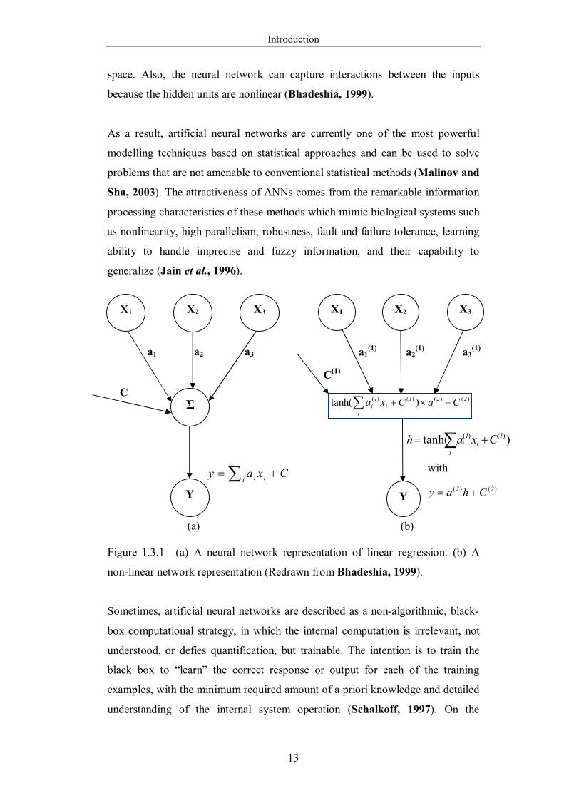
Figure 1.3.1 (a) A neural network representation of linear regression. (b) A
non-linear network representation (Redrawn from Bhadeshia, 1999).
…………..13
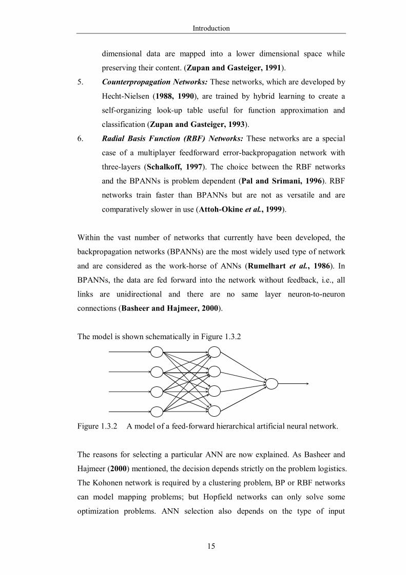
Figure 1.3.2 A model of a feed-forward hierarchical artificial neural network.
…………..15
Figure 1.5.1 Some explanations for an observed association. The broken lines
show an association. The arrows show a cause-and-effect link. The
variables x and y are under observation, and z is a lurking variable
(Redrawn from Moore and McCabe, 1999). ………………………….23
Figure 1.6.1 The electronegativity vs. the metallic radius for a coordination
number of 12 (Darken-Gurry) map for Ta as the solvent. (Taken from
Gschneidner and Verkade, 2004). ……………………………………34
Figure 1.6.2 (a) Darken-Gurry map for Mg as host metal. (b) Chelikowsky
method for Mg as host metal (Taken from Chelikowsky, 1979). ……...36
Figure 1.6.3 (a) Chelikowsky’s plot for the analysis of solid solubility in Fe;
…..38
(b) Alonso plot for analysis of solid solubility in Fe, the two
continuous lines separate the insoluble elements from the rest. (Taken
from Alonso and Simozar, 1980). ...…………………………………...39
Figure 1.6.4 The CALPHAD or phenomenological approach used to obtain a
thermodynamic description of a multicomponent system (Redrawn from
Chang et al., 2004). …………………………………………………….46
Figure 1.8.1 Global instability indices (GII) versus bond-valence based
tolerance factors (tBV) for ABO3-type perovskite compounds. (Redrawn
from Zhang et al., 2007). ………………………………………………55
Figure 1.9.1 Schematic arrangement of causation in materials science. ……..57
Figure 1.9.2 The interatomic distance – potential energy curve. …………….59
List of Figures
xi
Figure 3.2.1 Prediction of solubility using original values of input parameters
for the 60 alloy system dataset: atomic size, valency and electronegativity
and structure. a) Training set, b) Testing set, c) Whole set. ……………73
Figure 3.2.2 Prediction of solubility using 3 functionalized parameters for the
60 alloy system dataset: atomic size, valency and electronegativity. a)
Training set, b) Testing set, c) Whole set. ……………………………...74
Figure 3.2.3 Prediction of solubility using 4 functionalized parameters for the
60 alloy systems: atomic size, valence, electronegativity and structure. (a)
Training set, (b) Testing set, (c) Whole set. ……………………………75
Figure 3.2.4 The correlation between R-values and mean modulus of error. ..76
Figure 3.2.5 Prediction of solubility using 3 functionalized parameters for the
408 alloy systems: atomic size, valency and electronegativity. (a)
Training set, (b) Testing set, (c) Whole set. ……………………………78
Figure 3.2.6 Prediction of solubility using 3 functionalized parameters for the
60 alloy systems: valency, electronegativity and structure. (a) Training set,
(b) Testing set, (c) Whole set. …………………………………………..81
Figure 3.2.7 Prediction of solubility using 3 functionalized parameters for the
60 alloy systems: size, electronegativity and structure. (a) Training set, (b)
Testing set, (c) Whole set. ……………………………………………...81
Figure 3.2.8 Prediction of solubility using 3 functionalized parameters for the
60 alloy systems: size, valence and structure. (a) Training set, (b) Testing
set, (c) Whole set. ………………………………………………………82
Figure 3.2.9 Prediction of solubility using 2 functionalized parameters for the
60 alloy systems: size, valence. (a) Training set, (b) Testing set, (c)
Whole set. ………………………………………………………………85
Figure 3.2.10 Prediction of solubility using 2 functionalized parameters for the
60 alloy systems: size, electronegativity. (a) Training set, (b) Testing set,
(c) Whole set. …………………………………………………………...85
Figure 3.2.11 Prediction of solubility using 2 functionalized parameters for the
60 alloy systems: size, structure. (a) Training set, (b) Testing set, (c)
Whole set. ………………………………………………………………86
List of Figures
xii
Figure 3.2.12 Prediction of solubility using 2 functionalized parameters for the
60 alloy systems: valence, electronegativity. (a) Training set, (b) Testing
set, (c) Whole set. ………………………………………………………86
Figure 3.2.13 Prediction of solubility using 2 functionalized parameters for the
60 alloy systems: valence, structure. (a) Training set, (b) Testing set, (c)
Whole set. ………………………………………………………………87
Figure 3.2.14 Prediction of solubility using 2 functionalized parameters for the
60 alloy systems: structure, electronegativity. (a) Training set, (b) Testing
set, (c) Whole set. ………………………………………………………87
Figure 3.2.15 Prediction of solubility of 408 silver and copper alloy systems
using 3 functional parameters: atomic size, valence and electronegativity
and melting point of solvents and solutes. ……………………………...89
Figure 3.2.16 Prediction of solubility for 155 silver and copper alloy systems
using: (a) 3 funct ional parameters: atomic size, valence and
electronegativity; (b) melting points of solvents and solutes plus
parameters used in (a). ………………………………………………….91
Figure 3.2.17 Prediction of solubility for 231 noble metal alloy systems using: a)
3 functionalized parameters: atomic size, valence and electronegativity; b)
melting points of solvents and solutes plus parameters used in a). …….92
Figure 3.2.18 Prediction of Tmax for 155 silver and copper alloy systems using a)
3 functionalized parameters: atomic size, valence and electronegativity; b)
melting points of solvents and solutes plus parameters used in a); c)
melting points of solvents and solutes only. ……………………………95
Figure 3.2.19 Prediction of Tmax for 231 silver and copper alloy systems using a)
3 functionalized parameters: atomic size, valence and electronegativity; b)
melting points of solvents and solutes plus parameters used in a); c)
melting points of solvents and solutes only. ……………………………96
Figure 4.1.1 Prediction of a) enthalpy of vaporization from boiling point; b)
boiling point from enthalpy of vaporization; using data from CDH , LHC
and ELE. ………………………………………………………………103
List of Figures
xiii
Figure 4.1.2 Prediction of a) enthalpy of vaporization from boiling point; b)
boiling point from enthalpy of vaporization; using “consistent” data. ..114
Figure 4.1.3 Prediction of a) enthalpy of vaporization from boiling point; b)
boiling point from enthalpy of vaporization; using “consistent” data. ..120
Figure 4.1.4 Neural network fitting curves with ±10% boundaries for both
boiling point and enthalpy of vaporization prediction of the Category IV
dataset. ………………………………………………………………...120
Figure 4.1.5 Prediction of a) enthalpy of vaporization from boiling point; b)
boiling point from enthalpy of vaporization using dataset all recorded
from CES 2008. ……………………………………………………….126
Figure 5.2.1 (a) Prediction of global instability indices (GII) from bond-
valence based tolerance factors (tBV) for A1+B5+O3. …………………..135
Figure 5.2.1 (b) Prediction of global instability indices (GII) from bond-
valence based tolerance factors (tBV) for A2+B4+O3. …………………..135
Figure 5.2.1 (c) Prediction of global instability indices (GII) from bond-
valence based tolerance factors (tBV) for A3+B3+O3. …………………..136
Figure 5.2.1 (d) Prediction of global instability indices (GII) from bond-
valence based tolerance factors (tBV) for all type of ABO3 perovskite
compounds. ……………………………………………………………136
Figure 5.2.2 Global instability indices (GII) normalised by the valences of A-
site cations versus bond-valence based tolerance factors (tBV) for ABO3-
type perovskite compounds. …………………………………………..138
Figure 5.2.3 Prediction for perovskite formability of all ABO3-type compounds
from tBV and valences of A ions by ANN. …………………………….139
Figure 5.2.4 (a) Prediction for perovskite formability of the A1+B5+O3 by
ANN. ………………………………………………………..…………140
Figure 5.2.4 (b) Prediction for perovskite formability of the A2+B4+O3 by
ANN. ………………………………………………………..…………141
Figure 5.2.4 (c) Prediction for perovskite formability of the A3+B3+O3 by
ANN. ………………………………………………………..…………142
List of Figures
xiv
Figure 5.2.4 (d) Prediction for perovskite formability all type of ABO3 by
ANN. …………………………………………………………………..143
Figure 6.2.1 Results of prediction for polarizability with R values greater than
0.9, a) Prediction from atomic weight; b) Prediction from first ionization
potential; c) electronegativity; d) work function. ……………………..148
Figure 6.2.2 Result of prediction of polarizability using melting point, heat of
vaporization, specific heat capacity and first ionization potential. ……151
Figure 6.3.1 Variation of polarizability with atomic weight. ……………….153
Figure 6.3.2 Plots of work function versus atomic number (Drawn from the
values shown in Michaelson, 1950). ………………………………….155
Figure 6.3.3 Relation of experimental values of the work function to the
periodic system of the elements. (Drawn from the values shown in
Michaelson, 1977). …………………………………………………...156
Figure 6.3.4 Result of prediction of polarizability using atomic weight and
electronegativity. ……………………………………………………...165
Figure 6.3.5 Variation of polarizability as a function of atomic weight and
electronegativity. ……………………………………………………...166
Figure 6.3.6 Free vibration with damping curve. …………………………...167
Figure 6.3.7 Inverse function curve. ………………………………………..167
Figure 6.3.8 Plot of speculated function as shown in Equation 6.3.3. ……...169
Figure 6.3.9 Redrawn of Figure 6.3.5 from the same viewpoint and with the
same coloured as Figure 6.3.8. ……………………………………...169
List of Tables
xv
List of Tables
Table 1.6.1 Comparison of the prediction of solid solubilities by different methods
(redrawn from Zhang and Liao, 1999b). …………………………………...43
Table 1.7.1 Examples of inconsistent boiling point in handbooks and correct values
are underlined /K. ……………………………………………………………50
Table 1.7.2 Examples of inconsistent enthalpy of vaporization in handbooks, and
correct values are underlined /kJ mol-1 ………………………………………50
Table 3.2.1 Testing Hume-Rothery’s Rules with 60 alloy systems using his
criterion (14% variation), the later suggestion of 15% and the 15% c r i t e r io n
with structural identity (same or not). ……………………………………….72
Table 3.2.2 Comparison of criteria for predicting solubility using different
combinations of parameter groups. ………………………………………….79
Table 3.2.3 Comparison of criteria for predicting solubility using different
combinations of three parameters. …………………………………………...83
Table 3.2.4 Comparison of criteria for predicting solubility using different
combinations of two parameters. …………………………………………….88
Table 3.2.5 Statistical analysis of the results shown for Figure 3.2.16 and Figure
3.2.17. ………………………………………………………………………..93
Table 3.2.6 Statistical analysis of the results shown for Figure 3.2.18 and Figure
3.2.19. ………………………………………………………………………..97
Table 4.1.1 The dataset used to train the ANN shown in Figure 4.1.1. Majority
were taken from Chemistry Data Handbook (CDH, 1982) without judgement.
A few data unavailable in CDH were taken from LAG and ELE. (BP: Boiling
Point; ΔHV: Enthalpy of Vaporization). ……………………………………102
Table 4.1.2 List of boiling points from five handbooks (acronyms as in text).
Dataset does not have exclusions based on judgement. The elements are sorted
in ascending (Max.-Min.)/Min. …………………………………………….104
Table 4.1.3 List of enthalpies of vaporization from five handbooks (acronyms as in
text). Dataset does not have exclusions based on judgement. The elements are
sorted in ascending (Max.-Min.)/Min. ……………………………………..107
List of Tables
xvi
Table 4.1.4 List of Category I elements: boiling points of the elements are
consistent but enthalpy of vaporization are inconsistent. …………………..110
Table 4.1.5 List of Category II elements: enthalpies of vaporization are consistent
but boiling points are inconsistent. …………………………………………110
Table 4.1.6 List of Category III elements: both boiling point and enthalpy of
vaporization are inconsistent. ………………………………………………111
Table 4.1.7 List of Category IV elements: both boiling point and enthalpy of
vaporization are consistent. ………………………………………………...112
Table 4.1.8 The weights and biases of the network ANN1. …………………….113
Table 4.1.9 The weights and biases of the network ANN2. …………………….113
Table 4.1.10 List of Category I elements with predicted and selected correct values
of enthalpy of vaporization and difference percentage. ……………………115
Table 4.1.11 List of Category II elements with predicted and selected correct values
of boiling point and difference percentage. ………………………………...115
Table 4.1.12 List of Category III elements with predicted and selected correct values
and difference percentage (only the corrected pairs are shown). …………..118
Table 4.1.13 Statistical analysis for ANN performance in Figures 4.1.1, Figure 4.1.3
and Figure 4.1.5. ……………………………………………………………118
Table 4.1.14 List of Category II elements with predicted and selected correct values
of boiling point and difference percentage (with reference to normal boiling
point). ………………………………………………………………………128
Table 4.1.15 Systematic methodology for error checking in handbooks. ………..130
Table 6.2.1 Statistical analysis for the results shown in Figure 6.2.1. ………….149
Table 6.2.2 Statistical analysis for the results shown in Figure 6.2.2. ………….149
Table 6.3.1 Correlations between input properties. A strong correlation only exists
between melting point and heat of vaporization. …………………………..158
Table 6.3.2 Comparison of the criteria for predicting polarizability using different
combinations of three parameters. ………………………………………….160

List of Tables
xvii
Table 6.3.3 Comparison of the criteria for predicting polarizability using melting
point, heat of vaporization, and specific heat capacity respectively. ………160
Table 6.3.4 Comparison of the criteria for predicting polarizability using different
combinations of two parameters. …………………………………………...161
Introduction
1
1.0 Introduction 1.1 Aims and Objectives
Artificial neural networks (ANNs) represent one type of data mining procedure
and they have found acceptance in many subjects for modelling complex
problems. They have been applied in materials science for more than one decade
for finding the correlations between different materials parameters. The general
aim of this work is to explore correlations that might exist between different
properties in materials using ANN. Four distinct examples of their applications
are presented.
The objectives of this work are as follows:
1. To test whether it is feasible to predict solid solubility limits by using Hume-
Rothery’s Rules. If the result is positive, then to find what is the relative
importance of each rule, or to find the relative weighting and to assess how
well the weighted rules work for a) copper and silver alloys; b) a wider range
of alloys. If not, to find what other parameters are needed.
2. To discover a systematic, intelligent and potentially automatic method to
detect errors in handbooks and stop their transmission by using unrecognised
relationships between materials properties.
3. To make predictions of global instability index (GII) from bond-valence based
tolerance factors tBV for perovskites and to make the predictions of the
formability of perovskites by using A-O and B-O bond distance.
4. To explore the correlations that might exist between different properties
without knowing the direct structure-property relationships, and it is
exemplified by analyzing the correlation between polarizability and other
properties in detail.
Introduction
2
1.2 Approaches to Materials Science
In materials science it is important to establish the general composition-
processing-structure-property-performance relationships (Flemings, 1999), and
then allow the optimization of the processing parameters and compositions in
order to achieve the desired combination of properties for any particular
application (Malinov and Sha, 2003). These relationships can be obtained in the
following ways:
1) By experimental characterisation. The execution of well designed
experiments make it possible to get precise results which help to establish
structure-property relationship, but this is a time consuming and financially
costly procedure. Recently, experimental characterisation has been accelerated
by a method called combinatorial and high throughput materials development
and the details of these methods are discussed in part 1.2.1. These developments
result from a concern about the slow pace of conventional laboratory procedure.
2) By physical and empirical models. As set out by Bhadeshia (1999), a
theory can be judged by at least two criteria: 1) it must be able to describe a large
number of observations with few arbitrary parameters; 2) it must be able to make
predictions which can be verified or disproved. During the past decades, the
developments of theory on materials have helped greatly in understanding the
underlying phenomena. The further details are discussed in part 1.2.2.
3) By mathematical modelling. In terms of functionality, these approaches
can be classified into four categories: a) those which lead to unexpected
outcomes that can be verified; b) those which are created or used in hindsight to
explain diverse observations; c) existing models which are adapted or grouped to
design materials or processes; d) models used to express data, reveal patterns, or
for implementation in control algorithms (Bhadeshia, 2008; 2009). In terms of
the tools, they can be further subdivided into two classes: i) physical modelling
and ii) statistical modelling. Further details for physical modelling are discussed
in part 1.2.3 and statistical modelling is discussed in part 1.2.4.
Introduction
3
1.2.1 Combinatorial and High Throughput Methods
At the early stages of “science”, that is, before relationships between chemical
composition, crystal structure and material properties had been established,
artificial materials (artefacts) was produced by trial and error, known as pure
empiricism (Steurer, 1996). At present, the discovery of most new materials is
still solidly based in experimentation, although some progress has been made in
the ability to design or predict the properties of new materials. However, these
experimental approaches for materials development are being to be automated by
“high throughput” or “combinatorial” methods, which emerged as a response to
the challenges of materials development in increasingly complex experimental
spaces, i.e. the enormous number of possible combinations of composition, host
structure, dopants, defects, interfaces, processing conditions and so on, in an
attempt to increase the pace of materials development (Cawse, 2003). This kind
of methods are based on the construction of a library which may be thick or thin
film, continuous gradient, randomised or discrete (Dagani, 1999; Amis et al.,
2002; Zhao, 2006). Once a library has been created, it can be regarded as a
capital asset upon which a multitude of properties can be measured. It not only
make impressive successes in materials discovery, but also provide a new
paradigm for advancing a central scientific goal – the fundamental understanding
of structure-property relations of materials behaviour (Amis et al., 2002). Further,
the information obtained from such experiments can be used for converting the
data from high-throughput experimentation to high-throughput knowledge
discovery (Evans et al., 2001; Rajan, 2008).
The principle of this method can be traced to the 1960s when the groundbreaking
experiments in the field were first published. Kennedy et al. (1965) used a
ternary-alloy phase “library” produced by electron-beam co-evaporation
techniques and analyzed by electron diffraction, to successfully demonstrate
qualitative agreement between the phase diagram produced by combinatorial
techniques and that determined by conventional methods. In 1967, Miller and
Shirn (1967) analyzed the Au-SiO2 system by using a co-sputtering technique in
which a film exhibiting a controlled composition gradient of Au/SiO2 was
deposited on the substrate by aligning Au and SiO2 targets carefully. They then
used this gradient library to measure the electrical resistivity of the system over
Introduction
4
the full range of composition. In the following years, this “composition-spread”
method was used to study transition-metal-alloy superconductors (Hanak et al.,
1969; Sawatzky and Kay, 1969; Hanak, 1970).
Modern combinatorial chemistry appeared first in the 1980s in the
pharmaceutical industry (Borman, 1997). Geysen et al. (1984) helped jump-start
the field when his group developed a technique for synthesizing peptides on pin-
shaped solid supports; Richard (1985) developed a technique in which tiny mesh
packets act as reaction chambers and filtration devices for solid-phase parallel
peptide synthesis. After pioneering work done by Xiang et al. in 1995 (Xiang et
al., 1995), the interest in combinatorial materials sciences resurged. The work
after that included the search of superconductors (Xiang et al., 1995; Xiang,
1999; Amis et al., 2002), ferroelectrics (Schultz and Xiang, 1998; Murakami
et al., 2004), catalysts (Senkan, 1998; Jandeleit et al., 1999), dielectric
materials (Pullar et al., 2007a and 2007b) and for studying of phase diagrams
and composition-structure-property relationships (Zhao, 2006). At present, it can
be said that combinatorial methods not only make impressive successes in
materials discovery but also provide a new paradigm for advancing a central
scientific goal – the fundamental understanding of structure and property
relationships of materials behaviour (Amis et al., 2002).
However, it is also needs to be mentioned that this method is based on the
philosophy of Baconian science. It is important to notice that the words from
Francis Bacon (Bacon et al., 1905) were supposed to establish a philosophy of
science but William Harvey, who was one of the greatest experimental scientists
of that time, said that Bacon spoke of making observation, but omitted the vital
factor of judgment about what to observe and what to pay attention to (Feynman,
1969). As a result, essential analysis and judgments are needed after using the
high throughput data mining method.
1.2.2 Traditional Methodological Framework for Materials Science
In materials science, after the most simple binary and ternary alloys have been
studied, it becomes progressively more difficult, time consuming, and costly to
create useful new materials by using only experimental studies, so people have
Introduction
5
ambitions to predict material properties theoretically without experimentation
(Kawazoe, 1999). The traditional methodological framework for materials
science is the identification of the causal pathways that link composition and
structure to properties. The historical success of this approach is unquestioned.
The chemical composition is identifiable as the bulk elemental constituents as
determined to within a few molar percent by a range of analytical methods. For
some properties, ‘impurity’ or ‘dopant’ constituents which may be present at the
parts per million level have an effect on properties that is far out of proportion to
their concentrations. For example, in semiconductors and colorants, bulk
properties are strongly influenced by dopants; in ceramics, ‘impurities’ have a
pronounced effect on semiconduction and diffusion; conducting polymers can be
obtained by doping; and conducting polymer-matrix composites can be obtained
by the use of conducing fillers.
The structure of a material usually relates to the arrangement of its internal
components. Subatomic structure involves electrons within the individual atoms
and interactions with their nuclei; then, on atomic level, structure encompasses
the organization of atoms or molecules relative to one another; the next largest
structural realm, which contains large groups of atoms that are normally
agglomerated together is termed microscopic, which associated with grain
boundaries and stacking faults, also include point, line and planar defects such as
vacancies, substitutional and interstitial defects, dislocations, stacking faults,
twin and grain boundaries; finally, structural elements that may be viewed with
the naked eye are termed macroscopic, which includes pore size and fraction
(Callister, 2003).
Different levels of structures determine different kinds of properties:
1. The subatomic structure determines the chemical characteristics of elemental
materials (Mangonon, 1999).
2. Atomic structure influences the deformability of crystalline materials, like
metals and alloys.
3. Comparing with others, microstructure has strong effects on a large number of
material properties, such as I) Body centre cubic (BCC) structure is assumed
Introduction
6
to be more stable at higher temperature than the face centre cubic (FCC) or
hexagonal close packed (HCP) structure owing to its higher vibrational
entropy (Steurer, 1996); II) Incipient melting of metals occurs first at the
grain boundaries, which decreases the melting point; and grain boundaries
also enhance the creep deformation at high temperatures; III) At low
temperatures, the smaller the grain size of the material, the higher are its yield
strength, fracture strength, and toughness; IV) Two basic diffusion
mechanisms by which an atom moves in the structure are interstitial diffusion
which results from the interstitial defects, and vacancy diffusion which results
from substitutional defects or vacancies. Also, dislocations, grain boundaries
can enhance atomic movement; V) Dislocations allow crystalline materials to
be deformed into shapes, and make them more ductile compared with
materials that do not have dislocations or have sites that block dislocations.
4. Macroscopic structure, such as inclusions and cracks could influence transport
properties; and the overall component shape and size determine strengths.
The study of causation within the sequence composition-processing-structure-
properties is the traditional basis of the subject. Many of the successes in
materials science have emerged from its careful implementation. Many examples
of explaining properties from the structure are listed in textbooks. By using
fundamental principles of physics and chemistry that govern the states and
properties of condensed matter, as well as materials theory, it is possible to
model the structure and functional properties of real materials quantitatively, and
consequently to design and predict novel materials and devices with improved
performance (Elsässer et al., 2001).
1.2.3 Physical Modelling of Materials
Although it can be admitted that the scientific community at present is closer to
the realization of designing any material with given properties on the basis of
improved understanding of structure-property relationships (Steurer, 1996), the
development and processing of materials is complex, existing theories still lack
predictive power, i.e. the current level of theoretical and empirical understanding
of materials does not allow people to predict structures and hence the resulting
properties of the materials completely (Disalvo, 1990). As mentioned by
Introduction
7
Bhadeshia (1999), there remain many problems where quantitative treatments are
dismally lacking; and this incapability specially happens in the prediction of
mechanical properties, due to their dependence on large number of variables.
Examples are elastic modulus, yield strength, tensile strength, toughness, creep
strength, hardness and so on.
It is possible to predict properties by physical modelling. This method has been
characterized by multiscale; linking the simulation models and techniques across
the micro-to-macro length and time scales with the goal of analyzing and
controlling the outcome of critical materials processes. By combining different
modelling methods, such as quantum mechanical calculations, Monte Carlo
simulations, finite element analysis (FEA), the complex problems can be dealt
with in a much more comprehensive manner than when the methods are used
individually (Yip, 2005). These kinds of method are based on recognizing the
relationships between a structure and its properties: if a structure can be
calculated and optimized from given stoichiometries and connectivities, its
properties can be calculated as well (Fey, 1999).
Ab initio, or ‘first principles’ electronic structure calculations, is one typical
method; and are based solely upon 1) the laws of quantum mechanics, 2) the
masses and charges of electrons and atomic nuclei, and 3) the values of
fundamental physical constants, such as the speed of light or Planck’s constant
(Dorsett and White, 2000). The first ab initio calculation on a material was
done by Wigner and Seitz in 1934 (Wigner and Seitz, 1934) following their
previous paper, which is the first to apply the Schrödinger equation to the
problem of bonding in metals (Wigner and Seitz, 1933). At present, there is a
large number of commercial ab initio software packages available, such as
GAMESS, Dalton, Gaussian, Spartan, Chem3D, Material Studio, VASP, WIEN,
PWSCF, SIESTA, ADF, ABINIT, CPMD and Octopus. With these tools, the
number of diverse problems to which ab initio calculations have been directed is
very large (Cargnoni et al., 1998; Harrison et al., 1998; Milman et al., 2000;
Li, 2004; Van de Walle and Neugebauer, 2004; Music et al., 2007).
Introduction
8
Although ab initio calculations are theoretically the most rigorous, the techniques
that have been developed for solving these equations are extremely
computationally intensive (Yip, 2005). When large number of atoms (1023) and
the many-body interactions to be treated, this method would place a considerable
demand on computer resources (Kawazoe, 1999); and even when only a small
number of atoms are of interest, each step of the calculation may take several
hours on a multiprocessor machine (Chin et al., 2003). As mentioned by Pettifor
(2003), even with the largest parallel computer, only about 1000 non-equivalent
atoms can be simulated from first principles, which corresponds to a 3-D cell size
of about 1nm; and assuming the atoms are held together by some valence force
field or interatomic potential in order to simulate larger systems, only 1000
million atoms can be treated using the largest parallel computer, which
corresponds to a cell size of 0.1 μm. From comparing the highest computing
power recorded for year 2003 and at present from TOP500 (TOP500 website), it
is found that, even today, the cell size that can be treated is about 4 μm. However,
for nanomaterials, the reduction in size towards nanometric scales together with
the ever increasing computational power begin to allow direct application of ab
initio calculations to realistic systems (Lannoo, 2001), such as the work done by
Ordejón (2000).
At present, accompanying increasing computing power, several other techniques
have been developed for enhancing the resource efficiency and time for
computation such as 1) coarsening most of the details of the atomic or molecular
but retaining enough information for the essential physics to describe the
phenomena of interest, 2) employing multiprocessor computers and efficient
code parallelisation and 3) incorporating computational steering (Chin et al.,
2003). These make the simulation of systems that having length-scales of several
million atoms and timescales of up to milliseconds possible (Klein and Shinoda,
2008). Other examples for application of large-scale simulations that are free
from finite size effects can be found for layered materials (Suter et al., 2007;
Thyveetil et al., 2007; Suter et al., 2009). However, these simulations have the
capability to study a system of large number of atoms, but are not as reliable as
ab initio calculations (Dorsett and White, 2000; Yip, 2005).
Introduction
9
1.2.4 Statistical Modelling of Materials
When dealing with difficult problems where the physical models are not
available or tedious to apply, it is helpful to correlate the results with chosen
parameters by applying regression analysis, in which the data are best-fitted to a
specified relationship that is usually linear. The result of linear regression is an
equation, in which each of input xi is multiplied by a parameter ai; and the sum of
all such products and a constant C then gives an estimate of the output
i ii Cxay (Bhadeshia, 1999).
There are examples of applying linear regression method in materials sciences of
the type (Bhadeshia, 1999; 2009):
1) Cxaxaxay ii2211 ... Equation 1.2.1
This is a typical linear function and the idea is to predefined the function, then
correlate the empirically determined results against chosen variables using
regression analysis. One example for this kind of linear regression is the bainite
reaction start temperature (BS) in steel which can be written as:
MoCrNiMnCS C83C70C37C90C270830CB
where CC, CMn, CNi, CCr and CMo are the compositions of elements in wt.%,
typically C, Mn, Ni, Cr and Mo (Stevens and Haynes, 1956). However, in this
case, it needs to be pointed out that the physical model for BS has been found
later and the dependence on concentration of added elements is not linear
(Bhadeshia, 1981).
2) Cxaxaxay ii
221 ... Equation 1.2.2
Or the function can be like this, which is a pseudo-linear polynomial. The
example in material science is the basic thermodynamic parameter – heat
capacity at constant pressure (CP), which is expressed empirically as a function
of the absolute temperature T as follows:
Introduction
10
242
321P TaTaTaaC
As stated by Reid and Sherwood (1958), the prediction is usually based on
correlations of known information. These correlations can be classified as three
different types: purely empirical, partly empirical but based on some theoretical
concept, and purely theoretical. Within these, the first is often unreliable and may
not be worthy, the third is seldom adequately developed. The most widely used
correlations are of a form suggested in part by theory, with empirical constants
based on experimental data. Both of above two examples belong to the second
kind of correlations.
However, as mentioned by Specht (1991) and Bhadeshia (1999), there are
several difficulties associated with these general linear regression analysis: i) A
predefined relationship has to be chosen before analysis; ii) the chosen
relationship tends to be linear, or pseudo-linear with non-linear terms added
together and iii) when the regression equation once derived, it applied across the
entire span of the input space. However, it may not be a reasonable case; and so
the accuracy of predictions for unseen data would be low, as has been examined
in several people’s work (Bratchell et al., 1990; Barayani and Roberts, 1995;
Sofu and Ekinci, 2007; Moghtased-Azar and Zaletnyik, 2009).
Neural network, which falls in the statistical modelling category, can avoid the
difficulties that regression methods have. The details are discussed in what
follows.
Introduction
11
1.3 Artificial Neural Networks (ANNs)
1.3.1 Introduction to ANNs
The human brain is able to process information rapidly and efficiently through a
system of neural networks consisting of vast numbers of neurons. It has evolved
to enable a greater awareness of itself and its actions within its environment
(Amari, 2007). Compared with the programmed computing, in which (usually
procedural) algorithms are designed and subsequently implemented using the
currently dominant architecture, computation in the human brain is different in
that I) the computation is massively distributed and parallel, i.e. the basis of
biological computation is a small number of serial steps, each occurring on a
massively parallel scale; II) learning replaces a priori program development
(Schalkoff, 1997).
Taking these cues from nature, the biologically motivated computing paradigm
of artificial neural networks (ANNs) has arisen. Its appearance was determined
by two factors: one is the principal stages of the development of modern
elemental base technology that mainly determines the development of computer
architecture, and the second is the practical requirement to solve specific
problems in a faster and more economical manner. The main reason for the
development of neural computing since the 1950s appeared as a development of
the threshold logic which is in direct contrast to the classical development of the
elemental base on the basis of AND, OR, NOT and so on (Galushkin, 2007).
The ability to learn is a peculiar feature of intelligent systems. In artificial
systems, learning is viewed as the process of updating the internal representation
of the system in response to external stimuli so that it can perform a specific task.
ANN learning includes modifying the network architecture, which involves
incrementally adjusting the magnitude of the weights or, as it is known ‘synapse’
strength. This process is performed repetitively as the network is presented with
training examples, which is similar to the way that people learn from experience.
Then the ANN can generalize from the tasks it has learned to unknown cases
(Basheer and Hajmeer, 2000).
Introduction
12
Active research projects in the ANN field have been conducted by psychologists,
mathematicians, computer scientists, engineers, and others. It is considered that if
ANNs are to become a mature technology, the interfaces between existing
technologies and application areas such as modelling and simulation,
optimization theory, artificial intelligence, pattern recognition, and nonlinear
systems must be identified and unified. Like many engineering and scientific
disciplines, ANN system design often involves “trade-offs between exact
solutions to approximate models and approximate solutions to exact models”
(Schalkoff, 1997).
1.3.2 Comparison with General Regression Analysis
The comparison with general linear regression analysis can be illustrated by
Figure 1.3.1. The neural network also can represent linear regression, as shown
in Figure 1.3.1 (a). Here, each input xi is multiplied by a random weight ai and
the products are summed together with a constant C to give the output y. The
summation operates at the hidden node. Since initially, the weights ai and the
constant C are chosen at random, the output generally is not a match with
experimental data and so the weights are systematically changed, known as
training, until a best-fit description of the output is obtained as a function of the
inputs.
In comparison with that, the non-linear representation of neural networks is
shown in Figure 1.3.1 (b). In this case, the input data xi are multiplied by weights )(1
ia , and the sum of all these products forms the argument of a hyperbolic
tangent:
i
1i
1i Cxah )()(tanh , then )()( 22 Chwy . The choice of the
hyperbolic tangent function is due to its flexibility. The combination of more
than one hyperbolic tangent transfer function permits the ANN to capture almost
arbitrarily non-linear relationships; and the availability of a sufficiently complex
and flexible function means that the analysis is not as restricted as in linear
regression where the form of the equation has to be specified before the analysis.
The change of the exact shape of the hyperbolic tangent can be reached by
altering the weights, that is, hyperbolic function varies with position in the input
Introduction
13
space. Also, the neural network can capture interactions between the inputs
because the hidden units are nonlinear (Bhadeshia, 1999).
As a result, artificial neural networks are currently one of the most powerful
modelling techniques based on statistical approaches and can be used to solve
problems that are not amenable to conventional statistical methods (Malinov and
Sha, 2003). The attractiveness of ANNs comes from the remarkable information
processing characteristics of these methods which mimic biological systems such
as nonlinearity, high parallelism, robustness, fault and failure tolerance, learning
ability to handle imprecise and fuzzy information, and their capability to
generalize (Jain et al., 1996).
(a) (b)
Figure 1.3.1 (a) A neural network representation of linear regression. (b) A
non-linear network representation (Redrawn from Bhadeshia, 1999).
Sometimes, artificial neural networks are described as a non-algorithmic, black-
box computational strategy, in which the internal computation is irrelevant, not
understood, or defies quantification, but trainable. The intention is to train the
black box to “learn” the correct response or output for each of the training
examples, with the minimum required amount of a priori knowledge and detailed
understanding of the internal system operation (Schalkoff, 1997). On the
a3 a2 a1
C
X1 X2
Y
X3
Σ
i ii Cxay
X1 X2 X3
a3(1) a2
(1) a1(1)
C(1)
Y
)()()()( )tanh( 22
i
1i
1i CaCxa
)tanh( )()( i
1i
1i Cxah
with
)()( 22 Chay
Introduction
14
contrary, some people think neural network is transparent, consisting of an
equation and associated coefficients (the weights) and both the equation and the
weights can be studied to reveal the relationships and interactions. Due to the
nature of the interactions is implicit in the values of the weights and in some
cases there exist more than just pairwise interactions, the problems are difficult
to visualize from the examination of the weights. As a result, it is suggested that
a better method is to actually use the network to make predictions and to see how
these depend on various combinations of inputs (Bhadeshia, 1999).
At present, neural networks have been treated as wonderful tools that permit the
availability of quantitative expressions without compromising the known
complexity of the problem (Bhadeshia, 2009).
1.3.3 Types and Selection of ANNs
There are some frequently used ANNs from which to select. They have their own
characteristics and special applications:
1. Backpropagation Networks (BPANNs): This kind of network is versatile
and can be used in many fields such as data modelling, classification,
forecasting, control, data and image compression and pattern recognition
(Hassoun, 1995).
2. Hopfield Network: This kind of network is a symmetrical fully connected
two-layer recurrent network, which acts as a nonlinear associative
memory and is especially efficient in solving optimization problems
(Hopfield, 1984; Hopfield and Tank, 1986).
3. Adaptive Resonance Theory (ART) Networks: ART networks consist of
two fully interconnected layers, a layer that receives the inputs and a
layer consisting of output neurons. Like Hopfield networks, ART
networks can be used for pattern recognition, completion, and
classification (Basheer and Hajmeer, 2000).
4. Kohonen Networks: These networks are two-layer networks, which
transform n-dimensional input patterns into lower-ordered data where
similar patterns project onto points in close proximity to one another
(Kohonen, 1989). In addition to pattern recognition and classification,
Kohonen networks also can be used for data compression, i.e. high-
Introduction
15
dimensional data are mapped into a lower dimensional space while
preserving their content. (Zupan and Gasteiger, 1991).
5. Counterpropagation Networks: These networks, which are developed by
Hecht-Nielsen (1988, 1990), are trained by hybrid learning to create a
self-organizing look-up table useful for function approximation and
classification (Zupan and Gasteiger, 1993).
6. Radial Basis Function (RBF) Networks: These networks are a special
case of a multiplayer feedforward error-backpropagation network with
three-layers (Schalkoff, 1997). The choice between the RBF networks
and the BPANNs is problem dependent (Pal and Srimani, 1996). RBF
networks train faster than BPANNs but are not as versatile and are
comparatively slower in use (Attoh-Okine et al., 1999).
Within the vast number of networks that currently have been developed, the
backpropagation networks (BPANNs) are the most widely used type of network
and are considered as the work-horse of ANNs (Rumelhart et al., 1986). In
BPANNs, the data are fed forward into the network without feedback, i.e., all
links are unidirectional and there are no same layer neuron-to-neuron
connections (Basheer and Hajmeer, 2000).
The model is shown schematically in Figure 1.3.2
Figure 1.3.2 A model of a feed-forward hierarchical artificial neural network.
The reasons for selecting a particular ANN are now explained. As Basheer and
Hajmeer (2000) mentioned, the decision depends strictly on the problem logistics.
The Kohonen network is required by a clustering problem, BP or RBF networks
can model mapping problems; but Hopfield networks can only solve some
optimization problems. ANN selection also depends on the type of input
Introduction
16
(Boolean, continuous or a mixture of these) and the speed of the network once it
is trained. In the initial problem of simulating the process that Hume-Rothery
used to derive his rules (in object 1) the output is ‘soluble/insoluble’, and in the
prediction of the formation of perovskites (in object 3) the output is perovskite
formable/not, they are a kind of classification problems, and so the probabilistic
neural network (Specht, 1990; Vicino, 1998) is designed for use. This is a type
of radial basis network suitable for classification problems. In other works, the
problems all are mapping problems so backpropagation artificial neural networks
(BPANNs) are used.
1.3.4 Applications of ANNs in Materials Science
The application of neural networks in materials science at present is wide and it
has had a liberating effect on materials science by studying the diverse
phenomena which are not yet accessible to physical modelling. As afore cited,
the development and processing of materials is very complex and although
scientific investigations on materials have reached greater understanding of the
underlying phenomena, there still remain many problems where quantitative
treatments are dismally lacking. The lack of progress in predicting some
properties is because of their dependence on a large numbers of variables. Neural
networks are extremely useful in circumstances where the complexity of the
problem is overwhelming from a fundamental perspective and where
simplification is unacceptable (Bhadeshia, 1999).
There are some applications of neural networks in materials, and these
applications can be classified into two categories: 1) process control problems; 2)
materials properties prediction.
(1) Use of ANNs for process control
In Arkadan et al.’s work (1995), the location and shape of a crack were deduced
from measured magnetic field values as input. Raj et al. (2000) used ANNs in
metalworking to predict forging load in hot upsetting, cutting forces in
machining and loads in hot extrusion. Guessasma and Coddet (2004) used an
ANN to quantify the relationship between Automated Plasma Spraying process
parameters and microstructural features of aluminium-titanium coatings. Nam
Introduction
17
and Oh (1999) used a trained network to interpreted the output from sensors for
tracking the weld seam, and then to control a welding robot.
(2) Use of ANNs for materials properties prediction
It is the potential uses for prediction of properties of matter that is interesting for
materials scientists. The impact toughness of ferritic steel welds has been
predicted from the welding process, chemical composition, test temperature and
microstructure using neural networks (Bhadeshia et al., 1995). Homer et al.
(1999) used physical properties such as molecular weight, number of bonds and
temperature as input factors to predict the viscosity, density, enthalpy of
vaporization, boiling point and acentric factors for pure, organic, liquid
hydrocarbons over a wide range of temperatures (Treduced≈0.45-0.7). Huang et al.
(2002) predicted the mechanical properties of a ceramic tool based on materials
properties. Malinov and Sha (2004) used ANNs for correlation between
processing parameters and properties in titanium alloys such as fatigue life and
corrosion resistance. A three-layer backpropagation network ANN was applied to
the formulation of BaTiO3 – based dielectrics and for analysis of the electrical
properties of PZT (Guo et al., 2002; Cai et al., 2005).
Artificial neural networks have also been used in ceramic casting (Martinez et
al., 1994), to interpret ultrasonic NDT (Non-Destructive Testing) of adhesive
joints (Bork and Challis, 1995), for modelling the cold rolling forces (Larkiola
et al., 1996), to predict continuous-cooling transformation curves in steel from
chemical composition (Gavard et al., 1996) and to predict time-temperature
transformation diagrams for titanium alloys (Malinov et al., 2000). Bhadeshia et
al. recently reviewed applications of neural networks in the context of materials
science from their group and others (Bhadeshia, 1999; Bhadeshia, 2009;
Bhadeshia et al., 2009).
Introduction
18
1.4 Different Kinds of Scientific Methodologies
The application of neural networks in materials science will lead us to question
methodological procedures that are traditional in the discipline and which
originate from quite specific and strongly held views about scientific method. It
is appropriate, therefore to survey some of the principal positions in method in
order to chart our position.
The processes of evolution created neural networks in the brains of living
creatures. By reaching a certain degree of complexity, these networks generate
electrical phenomena in space and time called consciousness, volition and
memory. Such human brains have the capability to analyse the input signals
received from the world, in which they have their existence. One form of this
analysis, called science, has proved to be especially effective in correlating
modifying and controlling the sensory input data (Moore, 1972).
One view of scientific method, which is called conventionalism, or abduction in
logical terminology, states that the human mind created or invented certain
"beautiful" logical structures that are firstly defined as laws of nature, and then
devised some special ways of selecting sensory input data in order to fit into
patterns ordained by the laws, which are called experiments. In this view, the
scientists are like creative artists, working with the unorganized sensations from
a chaotic world such as paints or marbles. Philosophers like Poincaré (Poincaré,
1952), Eddington (Eddington, 1949), and Duhem (Duhem, 1985) support this
view.
A second view of science, which is called deductivism, also known as Popperian
science (Popper, 1963), is based on the creative emergence of hypotheses or
conjectures which gradually become well-trenched in the form of established
theories as more supporting experimental evidence is sought and found.
According to Popper’s definition (Popper, 1965), “Theories are nets cast to
catch what we call ‘the world’: to rationalize, to explain, and to master it. We
endeavor to make the mesh ever finer and finer.” In deductivists’ opinions, there
is no valid aposteriori logic, since general statements can never be proved from
particular instances. However, a general statement can be disproved by one
Introduction
19
contrary particular instance. As a result, a scientific theory can never be proved,
but it can be disproved. The role of an experiment is therefore to subject a
scientific theory to a critical test (Moore, 1972). Popper therefore emphasis
refutation to get around the problem of induction.
Another view of science, inductivism, preceded Popper by 350 years and was the
source of the problem Popper sought to solve. It is also known as Baconian
science, in which large amounts of data are firstly collected, assembled into
tables, surveyed and from which theories are devised. In his Novum Organum of
1620 (Bacon et al., 1905), Sir Francis Bacon argued that this was the only proper
scientific method. In fact, at that time, Bacon’s emphasis on observable facts was
an important antidote to medieval reliance on a formal logic of limited
capabilities. Although Bacon’s definition sounds close to the layman’s idea of
what scientists do, many competent philosophers have also continued to support
the essentials of inductivism, such as Russell (Russell, 1948) and Reichenbach
(Reichenbach, 1963).
A central debate in the history and philosophy of science focuses on the
contrasting explanations of scientific method from Popperian and Baconian
science, and Gillies (1996) has concisely articulated the contribution and impact
of artificial intelligence to philosophy of science: “…just as earlier the use of
instruments to assist observation altered the way in which science was done, so
the current development of computers and artificial intelligence is also destined
to change science, and in such a way that Baconian induction becomes a
standard part of scientific procedure.”
Introduction
20
1.5 Prediction, Causation and Inference
1.5.1 Cause-Effect, Contingency and Apophenia
The central aim of many studies in the physical, behavioural, social, and
biological sciences is the elucidation of cause-effect relationships among
variables or events. However, the appropriate methodology for extracting such
relationships from data, or even from theories, has been fiercely debated. There
are two fundamental questions of causality: I) What empirical evidence is
required for legitimate inference of cause-effect relationships? II) Given that the
causal information about phenomenon is willingly accepted, what inferences can
be drawn from such information, and how? But the fact is that these two
questions have been without satisfactory answers in part because people have not
had a clear semantics for causal claims and in part because people have not had
effective mathematical tools for casting causal questions or deriving causal
answers (Pearl, 2000).
David Hume, in taking an empiricist approach – that all knowledge can be
derived from sense experience rather than mind – made an important distinction
between statements that show the relationship between ideas (analytic) and those
that describe matters of fact (synthetic). He held the idea that people can accept
the idea of causality because it is a learnable habit of the imagination. The mind
records constant conjunctions based on past observations (Hume, 1896). This led
to the view that, when people say ‘A causes B’, it only means that A and B are
constantly conjoined in observation, rather than that there is some necessary
connection between them. He said that people have no other notion of cause and
effect, but that of certain objects, which have been always conjoined, and they
cannot penetrate further into the reason of the conjunction (Russell, 1996).
Hume's ideas of causality therefore have particular relation to the behaviour of
artificial neural networks whose main purpose is to find conjugations between
observations in the form of parameters in the form of correlations but to remain
silent on owning the mechanistic nature of the connection.
Contingency, based on the wider conception of association, was used to
substitute the idea of cause and effect. In the third edition of his book “The
Grammar of Science”, Pearson (1911) treated the law of causation as a
Introduction
21
conceptual figment extracted from phenomena, and not of their very essence.
The correlation between two occurrences is actually located in a category that
embraces different grades of association between two limits of absolute
independence (i.e. variation of the cause produces no effect on the phenomenon)
and absolute dependence (i.e. variation of the cause absolutely and alone varies
the phenomenon). That is, when a cause varies, a phenomenon changes, but to a
different extent; the less the variation in that change, the more nearly the cause
defines the phenomena and the more closely people assert the association or the
correlation to be. In this book, a contingency table was firstly used to analysis the
degree of association between variables by calculating a number of correlation
coefficients. Pearson believed the nature of the contingency table reflects the
essence of the association between cause and effect and “…the ultimate scientific
statement of description of the relation between two things can always be thrown
back upon such a contingency table…”. Pearson thus denies the need for an
independent concept of causal relation beyond correlation (Pearl, 2000).
Apophenia, which has been implicated in vulnerability to schizophrenia, is
defined as the tendency to perceive meaning in unrelated events. It is treated as a
“pervasive tendency of human beings to see order in random configurations”
(Brugger, 2001). However, whether it is a kind of over-mentalizing activity that
involves the dysfunction in the assessment of causality, or is a consequence of a
creative ‘hyper-associative style’ of intact causal reasoning still remains
speculative (Fyfe et al., 2008).
Apophenia can be treated as a behaviour that regards the coincidences of two
events as having cause-effect association. A coincidence is defined as “…a
surprising concurrence of events, perceived as meaningfully related, with no
apparent causal connection”, and it is the observer’s psychology that makes it
perceived, meaningful and apparent (Diaconis and Mosteller, 1989). Actually,
the coincidence can be studied and analysed by using statistical techniques, and
the possibility of coincidence occurring in random events can be precisely
predicted with the laws of probability (Diaconis and Mosteller, 1989; Falk and
Konold, 1997; Martin, 1998; Griffiths and Tenenbaum, 2001). In 1928,
Ramsey had proved that every large structure, such as large set of numbers,
Introduction
22
points or objects, contains a highly regular pattern, and complete disorder is an
impossibility (Graham and Spencer, 1990). Also as mentioned by Martin
(1998), the very nature of randomness assures that the combination of random
data will yield previous unknown patterns; however, people only can use it as a
hypothesis for investigating more data, but should never make a general
conclusion from it.
Also, apophenia can be treated as a powerful tool for creativity, in order to make
sense of the world. For creativity, the highest level is the production of a new
idea or theory which is completely distinct from and not conforming to or
deducible from any existing paradigm, and which is able to explain a wider range
of phenomena than any existing discovery. Historically, no discovery with great
importance was made by logical deduction, or by strengthening the observational
basis. As a result, random thinking is the most important element of creativity
(Rao, 1997). Also as Max Born once said “Science is not formal logic – it needs
the free play of the mind in as great a degree as any other creative art”.
1.5.2 Causation, Common Response and Confounding
When a strong association between variables is present, the conclusion that this
association is due to a causal link between the variables is often elusive. Figure
1.5.1 shows different underlying links between variables that can explain
observed association. The dashed line represents an observed association
between the variables x and y. Some association can be explained by a direct
cause-and-effect link between the variables. In Figure 1.5.1 (a), an arrow running
from x to y shows x “causes” y.
When thinking about an association between two variables, lurking variables
need to be considered. Figure 1.5.1 (b) illustrates common response, in which the
observed association between the variables x and y should be explained by a
lurking variable z; and both x and y change in response to changes in z. The
common response creates an association even though there may be no direct
causal link between x and y.
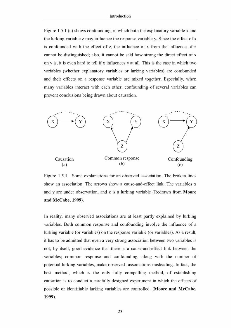
Introduction
23
Figure 1.5.1 (c) shows confounding, in which both the explanatory variable x and
the lurking variable z may influence the response variable y. Since the effect of x
is confounded with the effect of z, the influence of x from the influence of z
cannot be distinguished; also, it cannot be said how strong the direct effect of x
on y is, it is even hard to tell if x influences y at all. This is the case in which two
variables (whether explanatory variables or lurking variables) are confounded
and their effects on a response variable are mixed together. Especially, when
many variables interact with each other, confounding of several variables can
prevent conclusions being drawn about causation.
Figure 1.5.1 Some explanations for an observed association. The broken lines
show an association. The arrows show a cause-and-effect link. The variables x
and y are under observation, and z is a lurking variable (Redrawn from Moore
and McCabe, 1999).
In reality, many observed associations are at least partly explained by lurking
variables. Both common response and confounding involve the influence of a
lurking variable (or variables) on the response variable (or variables). As a result,
it has to be admitted that even a very strong association between two variables is
not, by itself, good evidence that there is a cause-and-effect link between the
variables; common response and confounding, along with the number of
potential lurking variables, make observed associations misleading. In fact, the
best method, which is the only fully compelling method, of establishing
causation is to conduct a carefully designed experiment in which the effects of
possible or identifiable lurking variables are controlled. (Moore and McCabe,
1999).
X Y Y Y X
Z Z
X
Causation (a)
Common response (b)
Confounding (c)
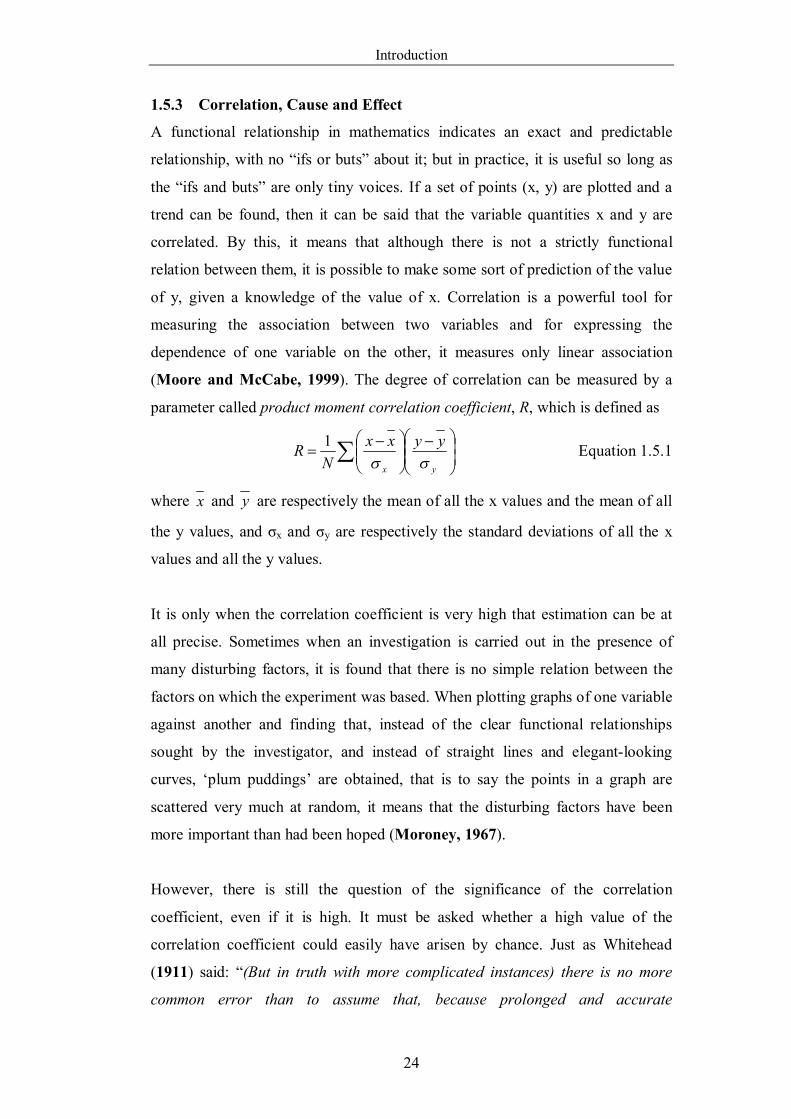
Introduction
24
1.5.3 Correlation, Cause and Effect
A functional relationship in mathematics indicates an exact and predictable
relationship, with no “ifs or buts” about it; but in practice, it is useful so long as
the “ifs and buts” are only tiny voices. If a set of points (x, y) are plotted and a
trend can be found, then it can be said that the variable quantities x and y are
correlated. By this, it means that although there is not a strictly functional
relation between them, it is possible to make some sort of prediction of the value
of y, given a knowledge of the value of x. Correlation is a powerful tool for
measuring the association between two variables and for expressing the
dependence of one variable on the other, it measures only linear association
(Moore and McCabe, 1999). The degree of correlation can be measured by a
parameter called product moment correlation coefficient, R, which is defined as
yx
yyxxN
R
1 Equation 1.5.1
where x and y are respectively the mean of all the x values and the mean of all
the y values, and σx and σy are respectively the standard deviations of all the x
values and all the y values.
It is only when the correlation coefficient is very high that estimation can be at
all precise. Sometimes when an investigation is carried out in the presence of
many disturbing factors, it is found that there is no simple relation between the
factors on which the experiment was based. When plotting graphs of one variable
against another and finding that, instead of the clear functional relationships
sought by the investigator, and instead of straight lines and elegant-looking
curves, ‘plum puddings’ are obtained, that is to say the points in a graph are
scattered very much at random, it means that the disturbing factors have been
more important than had been hoped (Moroney, 1967).
However, there is still the question of the significance of the correlation
coefficient, even if it is high. It must be asked whether a high value of the
correlation coefficient could easily have arisen by chance. Just as Whitehead
(1911) said: “(But in truth with more complicated instances) there is no more
common error than to assume that, because prolonged and accurate
Introduction
25
mathematical calculations have been made, the application of the result to some
fact of nature is absolutely certain”. Since the method of correlation analysis is
primarily used in cases where it is not possible to control the experimental
conditions, but such data as can be collected as they occur are analysed
(Moroney, 1967).
In the empiricist tradition, probabilistic relationships constitute the foundations
of human knowledge, whereas causality simply provides useful ways of
abbreviating and organizing intricate patterns of probabilistic relationships.
Causal relationships can be taken to be the fundamental building blocks both of
physical reality and of human understanding of that reality, and probabilistic
relationships can be regarded as but the surface phenomena of the causal
machinery that underlies and propels our understanding of the world (Pearl,
2000).
1.5.4 Causal and Analogical Connections
As people have tried to get to know nature’s forces and laws, they often applied
connections between different agents. These connections can be divided into two
types: 1) causal, that is the generation of one force by the other, which has been
mentioned above, and 2) analogical. While the causal connection links the forces
more tightly, analogical connection is helpful in understanding these forces and
in formulating theories. In history, both kinds of connections between electricity
and heat were exploited by those studying these phenomena. Ideas about these
connections were shaped by the changing concepts of the forces and by
experimental evidence for their interaction.
Ohm based his famous 1827 theory of the electric conduction of metals on
Fourier’s 1822 theory of heat flow. His success in deriving analogous equations
to those of Fourier for electric current indicated to him an “intimate connection”
between the two phenomena. Others then shared Ohm’s view. This view
stimulated Wiedemann and Franz to their discovery of an approximate constant
relation between the conductivity of heat and electricity in 1853. In turn, their
empirical law supported an assumption of the intimate connection between the
two phenomena, whose exact mechanisms were a subject of speculation until
Introduction
26
well after the discovery of the electron. Using a combination of empirical and
theoretical arguments, Lorenz claimed in 1872 that the Wiedemann-Franz
constant depends linearly on the temperature, a claim that he verified
experimentally by 1881. The electron theory of Drude explained Lorenz’s
relation on the assumption that both heat and electric currents in matter result
from the motion of its electrons (Shaul, 2005).
From this brief historically view, analogical connection is another kind of
association, which should be distinguished from causative associations.
Introduction
27
1.6 Developments and Applications of Hume-Rothery’s Rules
Hume-Rothery’s Rules, in the Baconian tradition, occupy a central space at the
heart of metallurgy. In the 1920’s, after surveying the available solubility data,
Hume-Rothery distinguished the factors that influence compound formation and
control alloying behaviour. There exists a connection between solubility, atomic
size, crystal structure and a particular concentration of valence electrons in an
alloy (Hume-Rothery, 1926; Massalski, 2000). Later, Hume-Rothery added
other ideas, and developed concepts which are now known collectively as Hume-
Rothery’s Rules (Hume-Rothery et al., 1934; Reynolds and Hume-Rothery,
1937; Hume-Rothery, 1967). There are already detailed reviews of Hume-
Rothery’s Rules, such as the work done by Massalski and King (1963),
Massalski and Mizutani (1978), Massalski (1996, 2000) and as described in
biographical sketches about Hume-Rothery (Pettifor, 2000a). Following the
hugely significant work by Hume-Rothery and his colleagues on the prediction
of solid solubility in alloys, many researchers contributed in different ways to the
prediction of solid solubility in terms of a soluble/insoluble criterion. The details
are discussed in part 1.6.1 and 1.6.2.
As cautioned by Pettifor (2000a), because different rules were expressed or
stressed by Hume-Rothery at different times, it is sometimes difficult to define
what constitutes ‘Hume-Rothery Rules’ and this confusion is extant. There is
general agreement that, in order of importance, the atomic size factor is first,
followed by the electronegativity effect. The importance of the electron
concentration (e/a ratio) in determining solid solubility boundaries is recognised
in some cases but other factors are rarely discussed in sufficient detail. Surveying
metallurgical and physical science publications in general, different sources
express Hume-Rothery’s ideas using terms such as: “effects”, “principles”,
“factors” or “parameters” (Massalski, 2000).
Researches on Hume-Rothery’s Rules blossomed in the 1930s-1980s but the
prediction of solubility was gradually superseded by calculation of phase
diagrams (CALPHAD), and the details are discussed in part 1.6.3. However, the
simplicity and generality of Hume-Rothery’s Rules still make them one of the
most important cornerstones in materials science. As mentioned by Watson and
Introduction
28
Weinert (2000), most of these rules are still useful today as in Hume-Rothery’s
time.
1.6.1 Early Formation and Revision of Hume-Rothery’s Rules
In 1926, after examining phase diagrams of the noble and related metals (i.e. Cu,
Ag and Au), especially those alloyed with the B-subgroup elements (including Li,
Be, B, C, N, O, F, Na, Mg, Al, Si, P, S, Cl, Zn, Ga, Ge, As, Se, Br, Cd, In, Sn, Sb,
Te, I, Hg, Tl, Pb, Bi), Hume-Rothery published a paper on the topic of compound
formation in several alloy systems (Hume-Rothery, 1926). In it, Hume-Rothery
predicted the β phase of Cu3Al would have the bcc structure because it satisfied
an electron per atom ratio of 3/2, which was confirmed one month later by
Westgren and Phragmén (1925).
In the 1930s, Hume-Rothery shifted his attention to characterisation of atomic
size by nearest neighbour distance instead of volume (Hume-Rothery, 1930). At
that time, two of the Hume-Rothery rules controlling solid solubility were
discovered: 1) the first Hume-Rothery rule, the atomic size factor, said that if the
atomic diameters of the solvent and solute differ by more than about 14-15%
then the primary solid solubility will be very restricted; 2) the second rule
emphasised the importance of the electron concentration (or electron per atom
ratio) in determining the phase boundary. Both of these rules are presented in his
classical paper in 1934 (Hume-Rothery et al., 1934).
In 1937, after studying the silver-rich antimony-silver alloy system with
Reynolds (Reynolds and Hume-Rothery, 1937), Hume-Rothery became aware
of a third factor restricting solid solubility, that is, electrochemical factor;
maximum solid solubility reduced as the electronegativity difference between
solute and solvent increased because of the competition to form intermetallic
compounds.
The relative valence rule was mentioned in the 1934 paper, and the importance of
this rule was stressed by Hume-Rothery in early editions of his famous book The
Structure of Metals and Alloys (Hume-Rothery, 1936). However, in his later
versions of this book, it is stated ‘more detailed examination has not confirmed
Introduction
29
this and, in its general form, the supposed principle must now be discarded’
(Hume-Rothery and Raynor, 1962; Hume-Rothery et al., 1969).
1.6.2 Further Developments and Applications of Hume-Rothery’s Rules
The development of Hume-Rothery’s Rules can be classified into two categories:
one is the development within each rule, and the other is the development of
anamorphoses or alternatives of these rules as a whole in order to get more
powerful and precise predictions.
1.6.2.1 Development and Application of Each Rule
Atomic Size Factor
The atomic size factor rule is usually presented in the following way (Hume-
Rothery et al., 1934): “if the atomic diameters of the solute and solvent differ by
more than 14%, the solubility is likely to be restricted because the lattice
distortion is too great for substitutional solubility.” When the size factor is
unfavourable, the primary solid solubility will be restricted; when the size factor
is favourable, other factors limit the extent of solid solubility and it is of
secondary importance. The size factor rule has been explained by using elastic
theory. It has be shown that (Friedel, 1954; Eshelby, 1956; Mott, 1962;
Cottrell, 1975), the ensuing total strain energy E in both solvent matrix and
solute can be estimated as
2308 rE Equation 1.6.1
where μ is the shear modulus and r0 and (1+ε)r0 are the unstrained radii of the
solvent and solute atoms. Taking ε as 0.14 (as the size factor rule declares) or
0.15, and 30r =0.7 eV, this gives TkE B4 at 1000 K. Darken and Gurry (1953)
proved that at temperature T, the primary solid solubility would be restricted to
below about 1 at.% when the energy of solution exceeds 4kBT per atom, where
kB is Boltzmann’s constant. Although elastic theory cannot be applied strictly at
the atomic level, this gives a simple explanation of Hume-Rothery’s size factor
rule. Also, Mott (1962) provided a quantum mechanical basis for this elastic
theory based on the Wigner-Seitz wave function ψ0(r), for an electron in the
lowest state in a Wigner-Seitz cell.
Introduction
30
The validity of the size factor has been debated since the rule was proposed.
Hume-Rothery et al. themselves (1934) pointed out that the exact “atomic
diameter” of an element is always difficult to define. They defined the atomic
diameter as given by the nearest-neighbour distance in a crystal of the pure metal.
However, this diameter cannot necessarily be transferred to the alloy because 1)
the ‘radius’ of an atom is probably affected by coordination number. Except for
the heavy elements, elements of the B sub-groups tend to crystallize with
coordination number 8-N, where N is the group to which the element belongs.
This is due to the partly covalent nature of the forces in these crystals and, except
in Group IV B, results in the atoms having two sets of neighbours at different
distances in the crystal. 2) In some structures there are great variations in the
closest distance between pairs of atoms at their closest distance of approach,
depending on the position and direction in the lattice. 3) On forming a solid
solution, the ‘sizes’ of individual atoms may change according to the nature and
degree of local displacements. In the case of anisotropic or complex structures or
where the coordination numbers are low, the closest distance of approach does
not adequately express the size of the atom when in solid solution (Massalski,
1996). Furthermore, atomic spacing increases or decreases as the composition
changes and so differences appear between the lattice spacing in alloys and the
estimated atomic sizes.
There are some attempts to derive the atomic size, such as extrapolating the size
variance trend of an element in the alloy towards the pure element to give a
hypothetical size (Axon and Hume-Rothery, 1948). Massalski and King (1963)
pointed out that in finding the atomic size factor, it is usually the volume per
atom that matters, not the distance between nearest neighbours, so they used the
change in volume per atom to obtain hypothetical dimensions.
The atomic dimensions can be calculated by using pseudopotential theory, such
as the work done by Hayes et al. (1968) on Li-Mg, Inglesfield (1969a; 1969b;
1969c) on Hg, Cd and Mg alloys, Hayes and Young (1970) on alkali alloys,
Stroud and Ashcroft (1971) for Cu-Al, Li-Mg and Cu-Zn, Meyer et al. (Meyer
and Young, 1969; Meyer et al., 1971a; Meyer et al., 1971b) on analyzing the
diffusion thermopowers of dilute alkali metal alloys, on calculating the lattice
Introduction
31
spacings and compressibilities of non-transition element solids and for analyzing
residual resistivities in silver and gold and Singh and Young (1972) on enthalpies
of solution at infinite dilution. They can also be obtained from the free-electron
model developed by Brooks (1963) and have been used by Magnaterra and
Mezzetti (1971; 1974).
The actual individual atomic sizes can also be estimated from static distortions in
a solid solution by modulation in diffuse X-ray scattering (Warren et al., 1951;
Roberts, 1954) or from weakening of the interference maxima analogous to
thermal effects (Huang, 1947; Herbstein et al., 1956; Borie, 1957; Borie, 1959).
From the analyses cited above, and as Cottrell (1998) suggested, the concept of a
characteristic size, which suggests hard spheres butted together is doubtful and
allocating a single atomic diameter for each element, independent of its
environment, and valences of solvent and solute is too simplistic an approach
(Hume-Rothery et al., 1969). At present, the importance of the size factor, of
course, extends far beyond primary solubility. Many intermetallic compounds
owe their existence to size-factor effects.
Relative Valence Factor
An early discovery by Hume-Rothery was that a metal of lower valence is more
likely to dissolve one of higher valence than vice versa. However, more
extensive investigation has not confirmed the generality of this rule. An example
is that monovalent silver can dissolve about 20% aluminium but trivalent
aluminium dissolves about 24% silver. However, for high valence, covalently
bonded components, the relative valence factor applies well. For example,
copper dissolves about 11% of silicon but silicon dissolves negligible copper
(Cottrell, 1998). This rule seems to be valid only when monovalent metals
copper, silver or gold are alloyed with the B-subgroup elements of the Periodic
Table which have higher valences. This is variously attributed to the partial
electron filling of the Brillouin zones in noble metals, the interaction of Fermi
surfaces and Brillouin zones in B-subgroup elements (Massalski, 1996) and
long-range charge oscillations around the impurity atoms (Hume-Rothery,
1961). Gschneidner (1980) implies that the relative valence effect is limited in
Introduction
32
applicability; when two high valence elements are alloyed it is not always
possible to predict which will form the more extensive solid solution with the
other.
Besides, the valencies of transition metals are variable and complex, as analysed
by Hume-Rothery et al. (1951) and Cockayne and Raynor (1961). Cottrell’s
book (1998) points out that due to the valency complication caused by partly
filled d orbitals, the transition metal alloys generally do not follow the rule.
Gschneidner (1980) revised the relative valence rule to suggest that the solubility
will be low if a metal in which d orbitals strongly influence the valence
behaviour is alloyed with a ‘sp metal’. The solubility is likely to be higher in the
d metal than the reverse.
Electronegativity Factor
The scale for electronegativity as given by Mulliken is based on the equation:
AI* 21 Equation 1.6.2
where I is the ionization energy, A is electron affinity, and * is Mulliken
electronegativity. Dividing by 2.8, gives approximately Pauling’s empirical scale.
Watson and Bennett (1978) point out that in the case of transition metals, the
partly filled d states at energies near the Fermi energy influence electronegativity.
They produced an electronegativity scale for transition metals, which matches
Pauling’s scale, and could be scaled by 2.8 to bring it to Mulliken’s scale.
As discussed by Hume-Rothery (1961), stable intermetallic compounds are prone
to form as the more electronegative is the solute and the more electropositive is
the solvent metal, or vice versa. Due to the lower free energy that can be
obtained when the system adopts a mixture of solid solution and compound,
solute atoms partition to form the stable compound rather than to enter solid
solutions. Further, as stated by Pearson (1972), in some binary alloy systems, if
one component is very electropositive relative to the other, there would be a
strong tendency for them to form compounds of considerable stability in which
valence rules are satisfied. This is the strongest effect in determining the
constitution of alloys, which dominates all other effects.
Introduction
33
Recently, Li and Xue (2006), on the basis of an effective ionic potential that is
defined in terms of ionisation energy and ionic radius, calculated the
electronegativities of 82 elements in different valence states and with the most
common coordination numbers, and pointed out that ‘although electronegativity
is often treated as an invariant property of an atom, as in Pauling’s scale, it
actually depends on the chemical environment of the atom, e.g. valence state,
coordination number and spin state’.
1.6.2.2 Mapping and Derivatives of Hume-Rothery’s Rules
While extensive efforts have been made to work out the theory behind the H-R
rules, it is very useful if the solubility of the materials can be mapped
diagrammatically on a Cartesian system. Thus researchers can simply calculate
the coordinate of the element to predict the solubility using such a diagram. This
direction started from Darken and Gurry (1953), followed by Chelikowsky
(1979), Gschneidner (1980), Alonso et al. (Alonso and Simozar, 1980; Alonso
et al., 1982), and Zhang and Liao (1999a; 1999b) among others.
Darken-Gurry Method
In 1953, Darken and Gurry (1953) proposed a diagrammatic method to describe
the solid solubility of fifty alloy systems (DG method). They used the size factor
as abscissa and electrochemical factor (electronegativity) as ordinate to plot
solubilities of each alloy system and then draw an ellipse to separate the soluble
elements from the insoluble elements, which is shown in Figure 1.6.1. The
solubility is characterized qualitatively as “extensive” or “limited”, inside the
ellipse or outside the ellipse, respectively.
Waber et al. (1963) examined the universality of the Hume-Rothery size rule and
the DG method for predicting solid solubilities. After analyzing 1455 binary
alloy systems, they confirmed Hume-Rothery’s size factor and showed that the
electronegativity is an important consideration in the formation of solid solutions.
In 1980, Gschneidner (1980) again applied the DG method to create a
soluble/insoluble classification by introducing the effect of crystal structure
(electronic-crystal structure Darken-Gurry method, ECSDG). Applying the
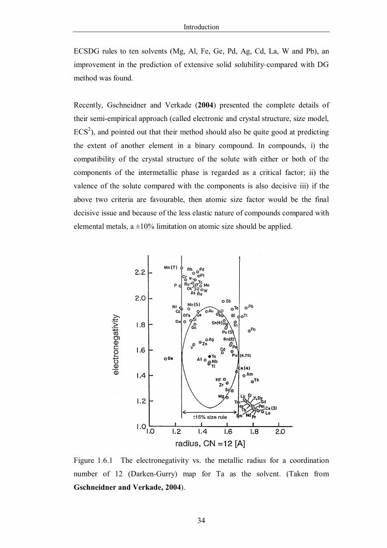
Introduction
34
ECSDG rules to ten solvents (Mg, Al, Fe, Ge, Pd, Ag, Cd, La, W and Pb), an
improvement in the prediction of extensive solid solubility compared with DG
method was found.
Recently, Gschneidner and Verkade (2004) presented the complete details of
their semi-empirical approach (called electronic and crystal structure, size model,
ECS2), and pointed out that their method should also be quite good at predicting
the extent of another element in a binary compound. In compounds, i) the
compatibility of the crystal structure of the solute with either or both of the
components of the intermetallic phase is regarded as a critical factor; ii) the
valence of the solute compared with the components is also decisive iii) if the
above two criteria are favourable, then atomic size factor would be the final
decisive issue and because of the less elastic nature of compounds compared with
elemental metals, a ±10% limitation on atomic size should be applied.
Figure 1.6.1 The electronegativity vs. the metallic radius for a coordination
number of 12 (Darken-Gurry) map for Ta as the solvent. (Taken from
Gschneidner and Verkade, 2004).
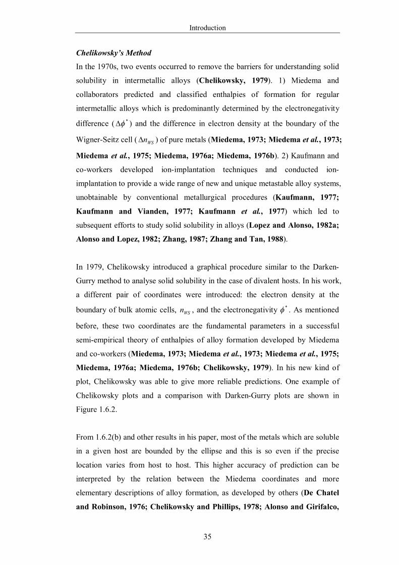
Introduction
35
Chelikowsky’s Method
In the 1970s, two events occurred to remove the barriers for understanding solid
solubility in intermetallic alloys (Chelikowsky, 1979). 1) Miedema and
collaborators predicted and classified enthalpies of formation for regular
intermetallic alloys which is predominantly determined by the electronegativity
difference ( * ) and the difference in electron density at the boundary of the
Wigner-Seitz cell ( WSn ) of pure metals (Miedema, 1973; Miedema et al., 1973;
Miedema et al., 1975; Miedema, 1976a; Miedema, 1976b). 2) Kaufmann and
co-workers developed ion-implantation techniques and conducted ion-
implantation to provide a wide range of new and unique metastable alloy systems,
unobtainable by conventional metallurgical procedures (Kaufmann, 1977;
Kaufmann and Vianden, 1977; Kaufmann et al., 1977) which led to
subsequent efforts to study solid solubility in alloys (Lopez and Alonso, 1982a;
Alonso and Lopez, 1982; Zhang, 1987; Zhang and Tan, 1988).
In 1979, Chelikowsky introduced a graphical procedure similar to the Darken-
Gurry method to analyse solid solubility in the case of divalent hosts. In his work,
a different pair of coordinates were introduced: the electron density at the
boundary of bulk atomic cells, WSn , and the electronegativity * . As mentioned
before, these two coordinates are the fundamental parameters in a successful
semi-empirical theory of enthalpies of alloy formation developed by Miedema
and co-workers (Miedema, 1973; Miedema et al., 1973; Miedema et al., 1975;
Miedema, 1976a; Miedema, 1976b; Chelikowsky, 1979). In his new kind of
plot, Chelikowsky was able to give more reliable predictions. One example of
Chelikowsky plots and a comparison with Darken-Gurry plots are shown in
Figure 1.6.2.
From 1.6.2(b) and other results in his paper, most of the metals which are soluble
in a given host are bounded by the ellipse and this is so even if the precise
location varies from host to host. This higher accuracy of prediction can be
interpreted by the relation between the Miedema coordinates and more
elementary descriptions of alloy formation, as developed by others (De Chatel
and Robinson, 1976; Chelikowsky and Phillips, 1978; Alonso and Girifalco,
Introduction
36
1979; Alonso et al., 1979; Alonso and Girifalco, 1978; Hodges, 1977; Hodges,
1978; Pettifor, 1979; Varma, 1979; Williams et al., 1980; Chelikowsky, 1982;
Gonzalez and Alonso, 1983; Lopez and Alonso, 1983; Lopez and Alonso,
1985; Gokcen et al., 1993). Recently, the Miedema parameters were used to
predict the formation of quasicrystals (Wang et al., 2003; Gui et al., 2006).
(a)
(b)
Figure 1.6.2 (a) Darken-Gurry map for Mg as host metal. (b) Chelikowsky
method for Mg as host metal (Taken from Chelikowsky, 1979).
Introduction
37
Although higher accuracy has been established, some exceptions remain. These
exceptions suggest that Chelikowsky’s method is still susceptible to some
improvement (Alonso and Simozar, 1980).
Alonso’s Method
In the 1980s, from analysis of both Darken-Gurry and Chelikowsky methods,
Alonso and Simozar (1980) proposed a scheme containing all three coordinates
(atomic size, electronegativity, electron cell-boundary density). The suggestion
was also proposed by Miedema and De Chatel (1980). By incorporating a size
factor in a new graphical method, they improved on the original Miedema
coordinate scheme proposed by Chelikowsky. In their analysis, each chemical
element is characterized by three parameters: the atomic volume V , the
electronegativity * , and the electron density at the boundary of bulk atomic
cells bn . * and wsn (the difference of electronegativity and electron density
at the boundary of bulk atomic cells) combined into a new parameter, CH , the
enthalpy of formation of an equi-atomic compound (Miedema et al., 1973;
Miedema, 1976b; Miedema et al., 1977). Then, the two parameters CH and
V (expressed as Wigner-Seitz radius, RW) are used to construct a two-
dimensional map. In this map, the chemical elements insoluble in a given host
are neatly separated from the soluble ones by a straight line. The examples and
the comparisons with Chelikowsky’s plot are shown in Figure 1.6.3 (a) and (b).
Later, Alonso et al. applied this method to the prediction of solid solubility in
noble metals, transition metals and sp metal based alloys (Alonso et al., 1982;
Lopez and Alonso, 1982). Jones has applied this method to the solid solubility
of two light metals, magnesium and aluminium (Jones, 1983).
After Miedema, the enthalpies of formation of different binary alloys have also
been predicted successfully from both first-principles and semi-empirical
methods (Maarleveld et al., 1986; Wei et al., 1987; Terakura et al., 1987;
Takizawa et al., 1989; Johnson, 1989; Ackland and Vitek, 1990; Johnson,
1990; Lu et al., 1991; Bozzolo and Ferrante, 1992; Bozzolo et al., 1992;
Sluiter and Kawazoe, 2002; Ouyang et al., 2003). During the last twenty years
and based on calculated enthalpies of formation of alloys and semi-empirical
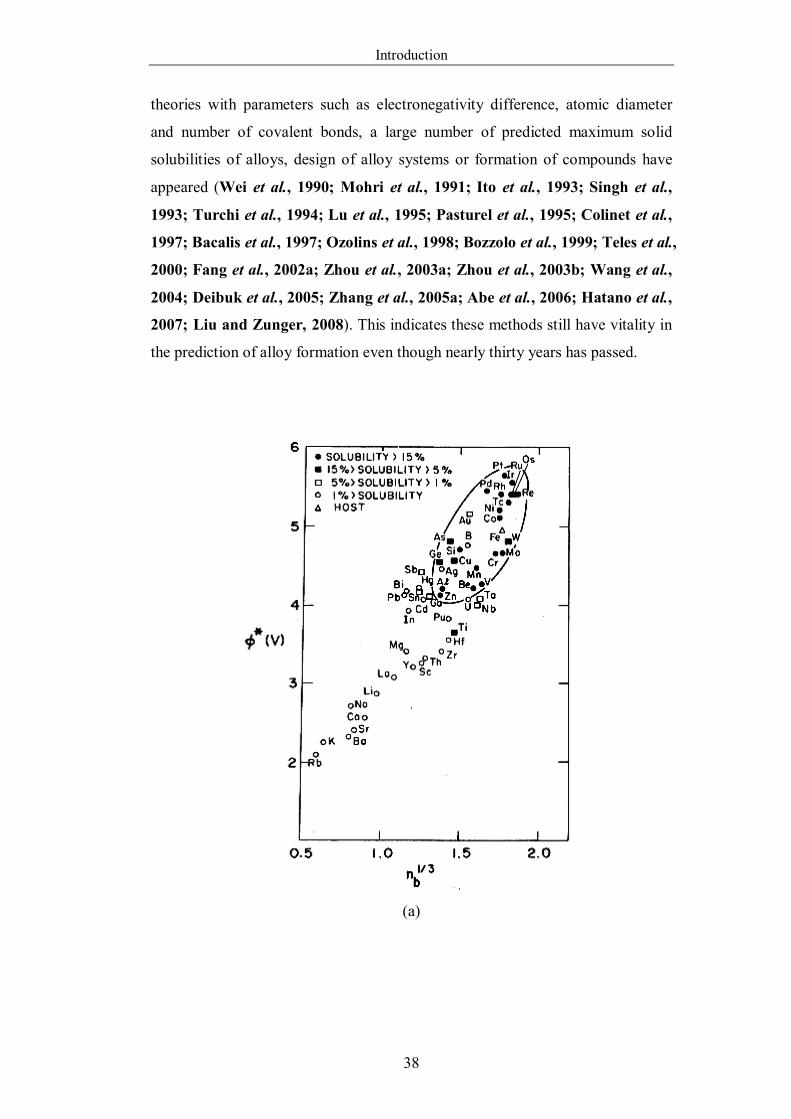
Introduction
38
theories with parameters such as electronegativity difference, atomic diameter
and number of covalent bonds, a large number of predicted maximum solid
solubilities of alloys, design of alloy systems or formation of compounds have
appeared (Wei et al., 1990; Mohri et al., 1991; Ito et al., 1993; Singh et al.,
1993; Turchi et al., 1994; Lu et al., 1995; Pasturel et al., 1995; Colinet et al.,
1997; Bacalis et al., 1997; Ozolins et al., 1998; Bozzolo et al., 1999; Teles et al.,
2000; Fang et al., 2002a; Zhou et al., 2003a; Zhou et al., 2003b; Wang et al.,
2004; Deibuk et al., 2005; Zhang et al., 2005a; Abe et al., 2006; Hatano et al.,
2007; Liu and Zunger, 2008). This indicates these methods still have vitality in
the prediction of alloy formation even though nearly thirty years has passed.
(a)
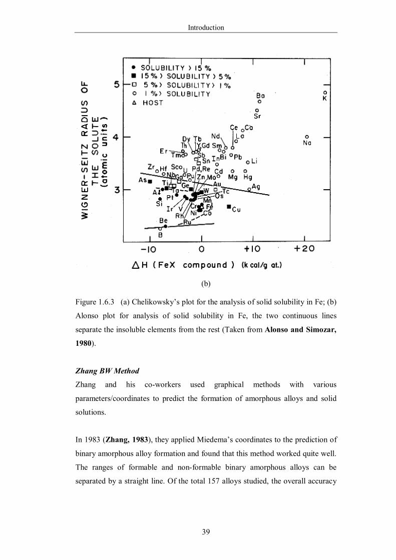
Introduction
39
(b)
Figure 1.6.3 (a) Chelikowsky’s plot for the analysis of solid solubility in Fe; (b)
Alonso plot for analysis of solid solubility in Fe, the two continuous lines
separate the insoluble elements from the rest (Taken from Alonso and Simozar,
1980).
Zhang BW Method
Zhang and his co-workers used graphical methods with various
parameters/coordinates to predict the formation of amorphous alloys and solid
solutions.
In 1983 (Zhang, 1983), they applied Miedema’s coordinates to the prediction of
binary amorphous alloy formation and found that this method worked quite well.
The ranges of formable and non-formable binary amorphous alloys can be
separated by a straight line. Of the total 157 alloys studied, the overall accuracy
Introduction
40
was 77.7%. These results compared well with the work done by Shi et al. (1979)
using bond-parametric diagrams, which had a prediction accuracy of 80%.
Taking the parameters used in Miedema’s coordinates without the size factor,
Zhang (1985a) combined the two chemical coordinates * and 3/1wsn into one:
1/13910 3/1* wsny Equation 1.6.3
and using the radius difference of elements
%1
21
RRRx
Equation 1.6.4
as the other coordinate to constructed a two-dimensional map. From this, the
definition of conditions for formation of binary amorphous alloys was improved.
The separation of the formable and non-formable regions was given by 75.105.0 xy . Of the total 157 alloys studied in that work, the overall accuracy
was 83.4%. It is found that the prediction accuracy for the formation of
amorphous alloys is improved when the size factor is added to the original
Miedema coordinates criterion.
Zhang and co-workers proposed another graphical method, which combined
bond parameters KrZ / and COVrZ / as an electron factor (where Z is atomic
valence, Kr is atomic kernel radius, equal approximately to the positive ionic
radius not including the valence electrons and COVr is covalent radius). Then,
together with a size factor to provide two coordinates for the study of solid
solubility, they described the formation of amorphous alloys (Zhang, 1981). The
two coordinates are expressed by (1) bond-parametric function
PPK
xrZx
rZ
32
31
cov
, where Px is the Pauling electronegativity; (2) half of
the empirical interatomic distance R respectively. When the coordinate point of a
host element is represented in the chart, the closer is the point of a solute element
to it, the smaller the differences of the electron factors and of the size factors
between the solute element and the host element. Zhang (1987b) applied this
method to 1080 binary and got a prediction accuracy of 93%.
Introduction
41
Zhang also used a modified electron factor
PBPAACOV
PABK
XXr
ZXrZy
32
31 Equation 1.6.5
as ordinate and %1
21
RRRx
as abscissa to search for solid solubilities at room
temperature in 2460 binary alloys. In this work the transition metals of the fourth,
fifth and sixth long periods and 18 non-transition metals are studied. For each
host element, a parabolic curve 2bxay can be drawn to separate the soluble
elements from the insoluble ones with a criterion of 0.5 at.% solubility at room
temperature. The overall reliability of this equation approached 90% for 2460
alloys. Also, it has been found that the values of a for each host metal are
proportional to its cohesive energies E, and b values are proportional to 30RE ,
where μ is the shear modulus of solvent element, and R0 is the atomic radius of
the solvent (Zhang, 1985b).
In 1996, Zhang and Liao (1996) applied this method to study the solid
solubilities for the binary alloy systems based on 13 rare earth metals, and found
the soluble elements can be separated from the insoluble ones by a parabola 211 bxay , where x1 is defined in equation 1.6.4 and, y1 is defined in equation
1.6.5 or an elliptical curve
1// 222
222 dnycmx Equation 1.6.6
where Rx 2 and
PP
K
xrZx
rZy
32
31
cov2
Equation 1.6.7
For the solid solubilities in 897 binary alloys, the prediction accuracy was 89.2%
for the parabolic separation, and 92.8% for the elliptical separation. Also, in the
elliptical equation, constants m and n were dependent on the coordinates 2x and
2y , c was proportional to 2/13 R and d was proportional E.
In 1999, Zhang and Liao (1999a; 1999b) summarized different methods used by
themselves and others and made a comparison in terms of prediction accuracy.
Those results are shown in Table 1.6.1.
Introduction
42
The ECS2 method, as well as Hume-Rothery’s rule and the Darken-Gurry
method, are for predicting solid solubility without considering Gibbs energy.
These methods are easy to use – needing only the physical parameters (radii,
electronegativity, structure) of two elements (Gschneidner and Verkade, 2004).
The extent of primary solid solubility can be derived by using first principle
calculations. Following work done by others (Olesinski and Abbaschian, 1986;
Zunger et al., 1990; Ansara I. et al., 1998; Fries and Jantzen, 1998; Yan and
Chang, 2000; Wolverton et al., 2002; Colinet, 2003), Shin et al. (2008)
described the Cu-Si system thermodynamically as an example of higher order
systems (i.e. solute elements in compounds) with first-principles calculations of
the ε-Cu15Si4 phase and solid solution phases. By considering the enthalpy of
mixing and Gibbs energies of individual phases in the Cu-Si binary system, it
was found that the existence of intermetallic compounds would strongly affect
solubility limits. Predictions of solid solubility of other alloy systems using first
principles can be found elsewhere (Fuks et al., 1975; Udovskii and Ivanov,
1977; Martin and Carstensen, 1981; Yamamoto et al., 1993; Luo et al., 1994;
Hallemans et al., 1994; Duschanek et al., 1995; Sluiter et al., 1996;
Flandorfer et al., 1997; Ding et al., 1999; Grobner et al., 1999; Ghosh et al.,
2002; Fang et al., 2002b; Song et al., 2003; Stuparevic, 2004; Van de Walle et
al., 2004; Tokunaga et al., 2006; Sluiter et al., 2006; Hallstedt and Kim, 2007;
Ghosh and Asta, 2007; Cao et al., 2008; Teyssier et al., 2008).
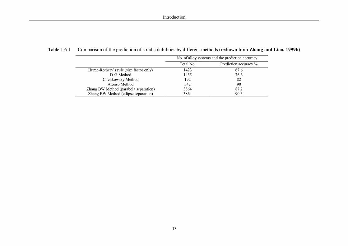
Introduction
43
Table 1.6.1 Comparison of the prediction of solid solubilities by different methods (redrawn from Zhang and Liao, 1999b) No. of alloy systems and the prediction accuracy
Total No. Prediction accuracy % Hume-Rothery’s rule (size factor only) 1423 67.6
D-G Method 1455 76.6 Chelikowsky Method 192 82
Alonso Method 342 90 Zhang BW Method (parabola separation) 3864 87.2 Zhang BW Method (ellipse separation) 3864 90.3
Introduction
44
1.6.3 Calculation of Phase Diagrams (CALPHAD)
Phase diagrams offer the most basic and important information on materials
systems, such as alloy systems. Traditionally, phase diagrams were determined
through doing experiments. For determination of the phase boundaries, the
specimens were heated over a sufficiently long time at an intended temperature
to achieve equilibrium. However, the problem is that the diffusivity of atoms is
generally not high enough at temperatures below half of the absolute Tm.
Therefore, it is not actually possible to conduct experiments on the phase
equilibrium below that temperature. On the other hand, special devices for
temperature control and atmosphere adjustment are required in experiments
conducted at extremely high temperatures. For these reasons, an explanation of
the entire phase diagram only from experimental work is rather difficult (Ohtani
and Ishida, 1998).
CALPHAD is an acronym for the CALculation of PHAse Diagrams, which aims
to couple the phase diagrams and thermochemical properties attempting
explicitly to characterise all of the possible phases in a system (Kaufman, 1998).
In detail, it is based on the well known thermodynamic law that a system with a
given composition, temperature and pressure attains the state of lowest Gibbs
energy under these given conditions; and if the Gibbs energy is known for the
individual phases, it is possible to calculate the equilibrium state by an energy
minimization procedure (Agren, 1996). The procedures of doing CALPHAD can
be illustrated as Figure 1.6.4.
The calculation of phase diagrams was started a century ago by Van Laar (1908a,
b) in which he calculated a great number of prototype binary phase diagrams
using ideal and regular solution models and then demonstrated the relationship of
the characteristic features of a binary phase diagram in terms of the relative
thermodynamic stabilities of the phases involved (Chang et al., 2004). This
situation remained unchanged for nearly half a century (Saunders and
Miodownik, 1998) before an alternative more physical approach based on band-
structure calculations (which stressed the electronic origin of solubility limits
only) was employed (Hume-Rothery et al., 1940). In the 1950s, Meijering
extended Van Laar’s methodology to higher order systems and calculated phase
Introduction
45
diagrams for ternaries using a regular solution model (Meijering, 1950; 1951;
Meijering and Hardy, 1956; Meijering, 1957; Meijering, 1960). Subsequently,
people started to calculate phase diagrams for real alloy systems, mostly for
binaries, using calculating machines, and then computers with software made by
themselves (Hillert, 1968; Pelton and Schmalzried, 1973; Sharma and Chang,
1979; Hillert, 1981; Lukas et al., 1982; Schmid, 1983; Chuang et al., 1985;
Chuang et al., 1986; Gabriel et al., 1987; Chuang and Chang, 1987; Chen et
al., 1989; Kattner et al., 1992; Murray et al., 1992; Chen and Chang, 1993).
Nowadays, the calculation of phase diagrams (CALPHAD) has been recognized
widely as a powerful tool that enables calculation of both stable and metastable
phase equilibria. Kaufman used a simple solution model to describe alloy phases
and systematically calculated phase diagrams for a large number of real alloy
systems, including binaries and some ternaries (Kaufman and Cohen, 1958;
Kaufman, 1959; Kaufman et al., 1963; Kaufman, 1969; Kaufman and Nesor,
1976; Kaufman, 1978; Kaufman and Nesor, 1978a, b, c, d; Kaufman, 1979a,
b; Kaufman and Tanner, 1979; Smith et al., 1980; Kaufman et al., 1981;
Kaufman and Tanner, 1984; Kaufman et al., 1984; Bouwstra et al., 1986;
Kaufman, 1991). Many of his early published results are summarised in the
monograph Computer Calculation of Phase Diagrams (Kaufman and Bernstein,
1970). Recently, more alloy systems have been evaluated (Lim et al., 1995;
Yang et al., 1995a; Zakulski and Moser, 1995; Yang et al., 1995b; Du and
Clavaguera, 1996; Gomez-A, 1998; Cui and Jin, 1999; Du et al., 1999; Du
and Yang, 2000; Ohnuma et al., 2000; Du et al., 2000; Liu et al., 2001; Fries
et al., 2001; Luo et al., 2001; Uhland et al., 2001; Kaufman et al., 2001;
Arroyave et al., 2002; Xiong et al., 2004; He et al., 2006; Guo et al., 2008;
Borzone et al., 2009).
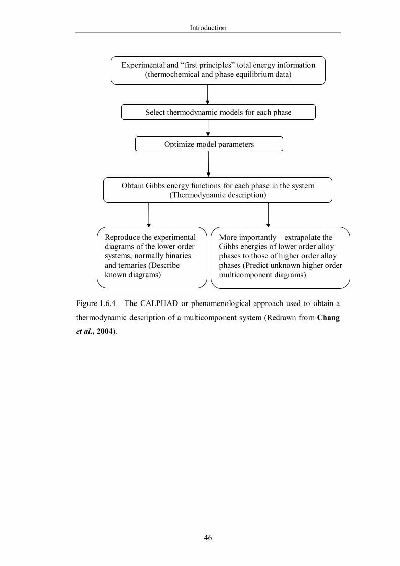
Introduction
46
Figure 1.6.4 The CALPHAD or phenomenological approach used to obtain a
thermodynamic description of a multicomponent system (Redrawn from Chang
et al., 2004).
Experimental and “first principles” total energy information (thermochemical and phase equilibrium data)
Select thermodynamic models for each phase
Optimize model parameters
Obtain Gibbs energy functions for each phase in the system (Thermodynamic description)
Reproduce the experimental diagrams of the lower order systems, normally binaries and ternaries (Describe known diagrams)
More importantly – extrapolate the Gibbs energies of lower order alloy phases to those of higher order alloy phases (Predict unknown higher order multicomponent diagrams)
Introduction
47
1.7 Errors in Handbooks and Databases
1.7.1 Error as a Fundamental Dimension of Data
Physical and chemical handbooks, some having long pedigrees and an increasing
number of databases are trusted for veracity of the data they contain. For a
database to have scientific value, it must meet criteria of completeness and
accuracy. However, as mentioned by Chrisman (1991), “error is inescapable, and
it should be recognized as a fundamental dimension of data”. The data entry
mistakes, faulty sensor readings or even more malicious activities provide a large
number of erroneous data sets, and then propagate these errors in each successive
generation of data (Hernández and Stolfo, 1998). As mentioned by Redman
(1997), error rates between 1% and 75% have been reported, and it is suggested
that unless extraordinary efforts are taken, dataset field error rates of 1-5% are
typically expected. Later it is reported that the error rates in the data acquisition
are generally about 5% or more (Orr, 1998; Redman, 1998). Another study
shows that as much as 40% of all collected data is dirty in one aspect or another
(Fayyad et al., 2003).
The collections in handbooks are assembled from other sources or manually
transcribed from earlier handbooks and the amount is always large. Errors (most
are typographical) are anticipated (Allen, 1998) and these errors are passed on,
rather like genetic mutations, into subsequent editions and newly written
handbooks and databases.
1.7.2 Existing Outlier Detection Methodologies
Outliers are defined as objects that do not comply with the general behaviour or
model of the data, and have different characteristic from or are inconsistent with
the remaining set of data (Agyemang et al., 2006; Han and Kamber, 2006).
In one aspect, outliers are treated as error or noise that must be removed. There
are various outlier-detection procedures to detect, and where appropriate, to
remove anomalous observations, such as contaminated data and errors (Hodge
and Austin, 2004). They have been applied to text data (Pollock and Zamora,
1984; Pfeiffer et al., 1996; Dalcin, 2005; Fan et al., 2008) and numerical data
(Walczak and Massart, 1998; Chalk et al., 2001). All of them need known
Introduction
48
functional correlations or dependencies. Presently, with the greatly enhanced
computing power available, several robust regression methods have been used to
detect and reject outliers (Liang and Kvalheim, 1996; Rousseeuw and Leroy,
2003; Colliez et al., 2006; Ortiz et al., 2006). Notably, in the materials science
field, statistical methods have been developed to estimate the veracity of material
properties (Ashby, 1998; Bassett et al., 1998). They seek out deviations from
predefined data ranges, correlations or fit the data to a function through
regression, and their performance is compared with the method used in this work
(part 4.3.4). In the other aspect, outlier detection also can be used to find rare and
interesting patterns for decision making, such as work done by Provost and
Aronis (1996), Chan et al. (1999), Liu et al. (2001), Shekhar et al. (2001),
Yamanish and Takeuchi (2002), He et al. (2002), Zhao et al. (2003), Petrovskiy
(2003), Kou et al. (2004), Jung and Jo (2004).
Milleer (1993), Bishop (1994), Markou and Singh (2003a, b), Hodge and Austin
(2004), Ben-Gal (2005), Maletic and Marcus (2005), Agyemang et al. (2006) and
Hand and kamber (2006) have surveyed different methods (e.g. statistical, neural
network, machine learning), used for outlier detection in different fields.
1.7.3 Policing and Correction of Errors by Exploring Correlations between
Properties
In this work, the procedure that has been devised is general for collections of
data in which hidden relationships can be found. It started out to see if ANNs can
discover unanticipated relationships between combinations of properties of
materials which might help identify potential compositional spaces for materials
discovery (part 1.9 and 6.0) and in doing so, discovered that the ANN is very
good at highlighting unusual data points in handbooks, tables and databases that
deserve to have their veracity inspected. It is also quite good at pointing an
accusing finger at the culpable values in a line-up of suspect data from different
sources. The outcome is a method of sifting large amounts of data to screen out
suspect values and the method could potentially be built into databases to form
an immune system providing the community with self-policing databases. The
method is based on the hypothesis that the data contains as-yet unknown
relationships which can be discovered by the ANN; established relationships are
Introduction
49
not essential. This work shows how correct data can be identified. Estimates can
easily be found for suspect data but this is quite unethical: as mentioned before,
outliers can act as a prompt for new discoveries. As mentioned by Han and
Kamber (2006), “In general, users must check that each outlier…is indeed a
‘real’ outlier.”
It is well known that both the boiling point and enthalpy of vaporization are very
important thermodynamic properties, which are required in processes involving
liquid and vapour phase transitions such as distillation, vaporization and drying
(Cachadiña and Mulero, 2007); as the result, the quality and veracity of these
data in handbooks play important roles for scientific community and industry.
In this work, a procedure was established, based on artificial neural networks
(ANNs), which finds remarkable levels of error in the records of properties of the
elements. Table 1.7.1 and 1.7.2 show examples of incorrect boiling point and
enthalpy of vaporization values discovered by ANN in elemental data; errors that
have persisted undetected into the 21st century. The representation of
abbreviations in tables are as follow: CDH: Chemistry Data Handbook (Stark
and Wallace, 1982); LAG: Lange’s Handbook of Chemistry (Speight, 2005);
ELE: The Elements (Emsley, 1998); TPC: Tables of Physical and Chemical
Constants (Kaye and Laby, 1995); CRC: CRC Handbook of Chemistry and
Physics (David, 2000).
In Table 1.7.2, some sources of error are self-evident when inconsistent data are
thus assembled: the difference in enthalpy of vaporization of Ho is about 4 times,
suggesting a missing conversion from calories to Joules; enthalpy of vaporization
of Ag and Al from TPC are 10 times smaller than the data from other sources,
implying a decimal point was incorrect. Sulphur and phosphorous are polyatomic
molecules, so the enthalpies of vaporization differ by a factor of 4.
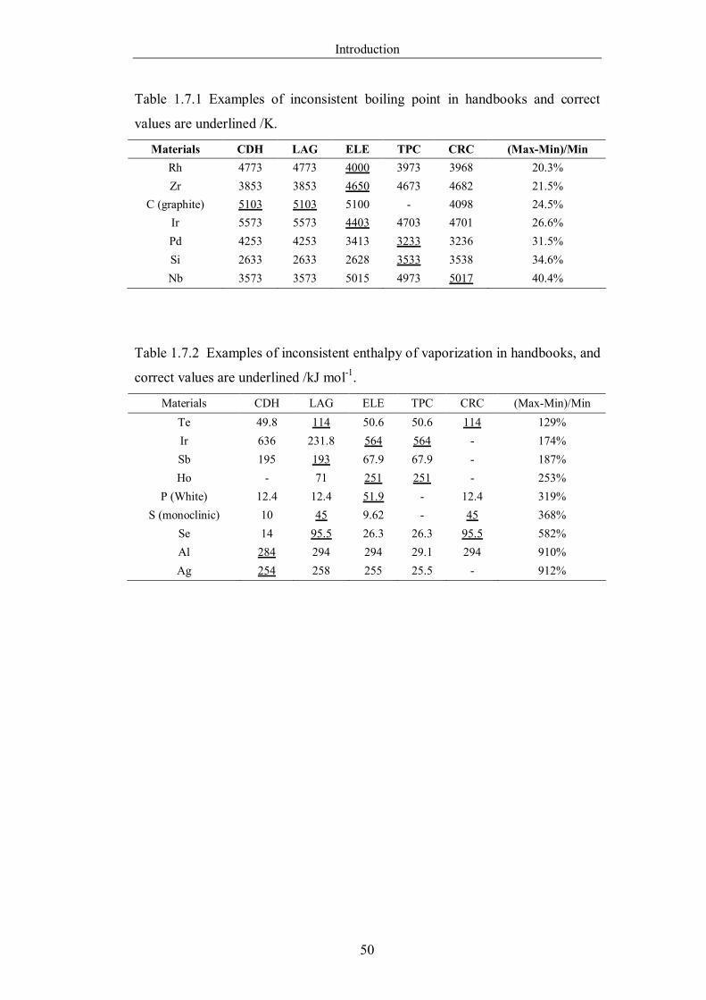
Introduction
50
Table 1.7.1 Examples of inconsistent boiling point in handbooks and correct
values are underlined /K.
Materials CDH LAG ELE TPC CRC (Max-Min)/Min Rh 4773 4773 4000 3973 3968 20.3% Zr 3853 3853 4650 4673 4682 21.5%
C (graphite) 5103 5103 5100 - 4098 24.5% Ir 5573 5573 4403 4703 4701 26.6% Pd 4253 4253 3413 3233 3236 31.5% Si 2633 2633 2628 3533 3538 34.6% Nb 3573 3573 5015 4973 5017 40.4%
Table 1.7.2 Examples of inconsistent enthalpy of vaporization in handbooks, and
correct values are underlined /kJ mol-1.
Materials CDH LAG ELE TPC CRC (Max-Min)/Min Te 49.8 114 50.6 50.6 114 129% Ir 636 231.8 564 564 - 174% Sb 195 193 67.9 67.9 - 187% Ho - 71 251 251 - 253%
P (White) 12.4 12.4 51.9 - 12.4 319% S (monoclinic) 10 45 9.62 - 45 368%
Se 14 95.5 26.3 26.3 95.5 582% Al 284 294 294 29.1 294 910% Ag 254 258 255 25.5 - 912%
Introduction
51
1.8 The Prediction of Structural Stability and Formation of ABO3-type
Perovskite compounds
1.8.1 Crystal Structure Determination
Crystal-structure and materials properties are intimately linked together, so
obtaining information on crystal structures continues to be an area of ongoing
research. Presently, crystallographic information is a prerequisite for any
extensive materials modeling and so knowledge of crystal structures is a practical
and pressing quest (Morgan and Ceder, 2005)
There are three main approaches for determination of crystal structures. (1)
Experimental determination: such work began in 1911 by von Laue and his
colleagues (Friedrich et al., 1912); and Bragg (1913). The experimental
approach is expensive despite the emergence of high throughput automation
(Kennedy et al., 1965; Xiang et al., 1995), as mentioned before. (2) The
evolution of high-speed computers and the derivation of one-electron potentials,
which greatly simplify many-body interactions, make it possible to predict
structures using quantum mechanics principles, as demonstrated by Wolverton et
al. (2002), Asta et al. (2001), Blum and Zunger (2004) and Curtarolo et al.
(2005). These modelling efforts have made computational materials design a real
possibility but difficulties still exist: i) As Chelikowsky (2004) wrote: “Although
the interactions in … compounds are well understood, it is not an easy task to
evaluate the total energy of solids … As the energy of an isolated atom is in the
order of about 106 eV, but the cohesive energy only in the order of about 1-10
eV/atom, one must have a method that is accurate to one part on 106, or better.” ii)
The number of particles involved complicates the situation of evaluating the
cohesive energy and makes such computations less accurate than experiment
(Villars, 2000). (3) With the help of databases of known structures or models
which have physical meaning, certain regularities, such as laws, rules, principles,
factors, tendencies or patterns, might be found to help predict unknown
structures. This approach, known as structure mapping, is one of the more
successful non-experimental methods for crystal structure prediction and has
been reviewed by Burdett and Rodgers (1994), Villars (2000) and Pettifor
(2000b). Examples of structure mapping include Mooser-Pearson Maps (1959),
Zunger Maps (1980), and Villars Maps (1983, 1984a, b), but the best known are
Introduction
52
Pettifor Maps (1984, 1986). This method orders the very large database into
domains of different structure types and can be used as an initial guide in the
search for new compounds with a required structure type.
1.8.2 Data Mining Methods in Crystal Structure Prediction
The data mining (DM) method has become a powerful tool in different branches
of materials science offering the possibility of making descriptive and even
quantitative predictions in many areas where traditional approaches have had
limited success. Generally, predictions are made through constitutive relations,
that is, derived mathematically from basic laws of physics; however, in many
cases, the problems are so complex that constitutive relations either cannot be
derived or are too approximate or intractable for practical quantitative use. The
data mining method is based on the assumption that the useful constitutive
relations exist, and can be derived primarily from data rather than from basic
laws of physics (Morgan and Cerbrand, 2005).
Because there is no generally reliable and tractable method to predict structure,
and taking into account that a lot of structural data exist in crystallographic
databases such as ICSD (Bergerhoff et al., 1983), Linus Pauling files (Villars et
al., 1998), CRYSTMET (White et al., 2002), and others as mentioned in the
review paper by Allen (1998), crystal structure prediction is an area well suited
for data mining. Examples include works by Woodley et al. (1999), Curtarolo et
al. (2003), Fischer et al. (2006), Kazius et al. (2006) and, in particular, Morgan
et al. (2003), who developed a clustering algorithm to automate the construction
and testing of Pettifor maps based on data from a materials crystal structure
database.
1.8.3 Structural Stability and Formation of ABO3-type Perovskite
Compounds
The physical and chemical properties of perovskite and perovskite-related
materials are diverse and can be applied in a variety of fields, so it is useful to
discover the regularities that govern the formation of perovskite-type compounds
in order to guide the exploration of new materials in the huge compositional
spaces available (Zhang et al., 2007).
Introduction
53
The study of ABO3 compounds has a long history. Megaw (1946) accurately
determined the structure of a number of doubled perovskites by examining high-
angle lines on X-ray powder photographs. Salinas-Sanchez et al. (1992)
introduced a parameter called the global instability index (GII), which can be
used to determine the overall structural stability of perovskites. Giaquinta and
Loye (1994) later predicted the perovskite structure for a number of compounds
based on the combination of ionic radii and bond ionicities, predicting the
structure of InMO3 (M = Mn, Fe) with this method. Reaney and Ubic (1999)
reviewed the relationship between the tolerance factor (t) and the temperature
coefficient of permittivity (τε) (and therefore resonant frequency, τf) in
perovskites and also discussed the effect on τε of changing t in the perovskite-
related solid solution series Ba6-3xNd8+2xTi18O54. Lufaso and Woodward (2001)
used a bond-valence model to calculate ideal A – X and B – X bond distances in
order to calculate the bond-valence based tolerance factor (tBV) which they
proposed as a new criterion of the structural stability of ABO3-type perovskite
compounds. Ye et al. (2002) applied a pattern recognition method and found
some regularities in the formation and the lattice distortion of perovskites. Li et
al. (2004) used rA – rB structure maps to study the perovskite formability of 197
ABO3 compounds and then, with the knowledge of the importance of the
octahedral factor (rB/rO) and tolerance factor ()(2 OB
OA
rrrr
), another structure
map was constructed to predict the perovskite formability. Jiang et al. (2006)
investigated the regularities governing lattice constant of ABX3-type compounds
by a statistical regression method and found a good correlation among lattice
constant, the estimated bond length between ion B and ion X (rB + rX) and the
ionic-radii tolerance factor tIR; however, they used ionic radii of all ions A, B and
X appropriate for sixfold coordination, which are inappropriate for A and X.
Ubic (2007) later used a different approach based solely on ionic size and
derived a simpler and more accurate empirical relationship between ionic size
and lattice constant. In 2007, Zhang et al., based on the bond-valence model
(BVM) and structure-map technology, investigated the structural stability and
formability of ABO3-type perovskite compounds, established new criteria for the
structural stability of such compounds, and created new structure maps that can
be used for exploring novel perovskite-related compounds. In that work, the
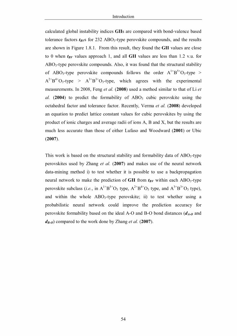
Introduction
54
calculated global instability indices GIIs are compared with bond-valence based
tolerance factors tBVs for 232 ABO3-type perovskite compounds, and the results
are shown in Figure 1.8.1. From this result, they found the GII values are close
to 0 when tBV values approach 1, and all GII values are less than 1.2 v.u. for
ABO3-type perovskite compounds. Also, it was found that the structural stability
of ABO3-type perovskite compounds follows the order A1+B5+O3-type >
A2+B4+O3-type > A3+B3+O3-type, which agrees with the experimental
measurements. In 2008, Feng et al. (2008) used a method similar to that of Li et
al. (2004) to predict the formability of ABO3 cubic perovskite using the
octahedral factor and tolerance factor. Recently, Verma et al. (2008) developed
an equation to predict lattice constant values for cubic perovskites by using the
product of ionic charges and average radii of ions A, B and X, but the results are
much less accurate than those of either Lufaso and Woodward (2001) or Ubic
(2007).
This work is based on the structural stability and formability data of ABO3-type
perovskites used by Zhang et al. (2007) and makes use of the neural network
data-mining method i) to test whether it is possible to use a backpropagation
neural network to make the prediction of GII from tBV within each ABO3-type
perovskite subclass (i.e., in A1+B5+O3 type, A2+B4+O3 type, and A3+B3+O3 type),
and within the whole ABO3-type perovskite; ii) to test whether using a
probabilistic neural network could improve the prediction accuracy for
perovskite formability based on the ideal A-O and B-O bond distances (dA-O and
dB-O) compared to the work done by Zhang et al. (2007).
Introduction
55
-0.10
0.10.20.30.40.50.60.70.80.9
11.11.21.31.41.5
0.8 0.85 0.9 0.95 1 1.05 1.1 1.15
t BV
GII
(v.u
.)
A¹⁺B⁵⁺O₃
A²⁺B⁴⁺O₃
A³⁺B³⁺O₃
Figure 1.8.1 Global instability indices (GII) versus bond-valence based
tolerance factors (tBV) for ABO3-type perovskite compounds. (Redrawn from
Zhang et al., 2007).
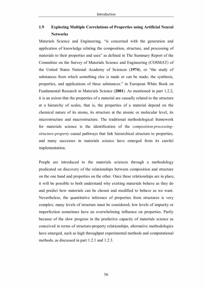
Introduction
56
1.9 Exploring Multiple Correlations of Properties using Artificial Neural
Networks
Materials Science and Engineering, “is concerned with the generation and
application of knowledge relating the composition, structure, and processing of
materials to their properties and uses” as defined in The Summary Report of the
Committee on the Survey of Materials Science and Engineering (COSMAT) of
the United States National Academy of Sciences (1974), or “the study of
substances from which something else is made or can be made; the synthesis,
properties, and applications of these substances.” in European White Book on
Fundamental Research in Materials Science (2001). As mentioned in part 1.2.2,
it is an axiom that the properties of a material are causally related to the structure
at a hierarchy of scales, that is, the properties of a material depend on the
chemical nature of its atoms, its structure at the atomic or molecular level, its
microstructure and macrostructure. The traditional methodological framework
for materials science is the identification of the composition-processing-
structure-property causal pathways that link hierarchical structure to properties,
and many successes in materials science have emerged from its careful
implementation.
People are introduced to the materials sciences through a methodology
predicated on discovery of the relationships between composition and structure
on the one hand and properties on the other. Once these relationships are in place,
it will be possible to both understand why existing materials behave as they do
and predict how materials can be chosen and modified to behave as we want.
Nevertheless, the quantitative inference of properties from structures is very
complex; many levels of structure must be considered; low levels of impurity or
imperfection sometimes have an overwhelming influence on properties. Partly
because of the slow progress in the predictive capacity of materials science as
conceived in terms of structure-property relationships, alternative methodologies
have emerged, such as high throughput experimental methods and computational
methods, as discussed in part 1.2.1 and 1.2.3.
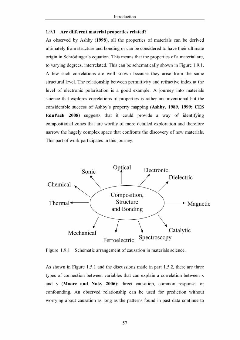
Introduction
57
1.9.1 Are different material properties related?
As observed by Ashby (1998), all the properties of materials can be derived
ultimately from structure and bonding or can be considered to have their ultimate
origin in Schrödinger’s equation. This means that the properties of a material are,
to varying degrees, interrelated. This can be schematically shown in Figure 1.9.1.
A few such correlations are well known because they arise from the same
structural level. The relationship between permittivity and refractive index at the
level of electronic polarisation is a good example. A journey into materials
science that explores correlations of properties is rather unconventional but the
considerable success of Ashby’s property mapping (Ashby, 1989, 1999; CES
EduPack 2008) suggests that it could provide a way of identifying
compositional zones that are worthy of more detailed exploration and therefore
narrow the hugely complex space that confronts the discovery of new materials.
This part of work participates in this journey.
Figure 1.9.1 Schematic arrangement of causation in materials science.
As shown in Figure 1.5.1 and the discussions made in part 1.5.2, there are three
types of connection between variables that can explain a correlation between x
and y (Moore and Notz, 2006): direct causation, common response, or
confounding. An observed relationship can be used for prediction without
worrying about causation as long as the patterns found in past data continue to
Composition, Structure
and Bonding
Sonic Optical Electronic
Dielectric
Magnetic
Catalytic Spectroscopy Ferroelectric
Mechanical
Thermal
Chemical
Introduction
58
hold true. The purpose of exploring a correlation is to make predictions, which
are usually based on correlation of known information, with interpolation or
extrapolation as required.
1.9.2 Examples of Known Correlations between Properties
The idea of exploring property-property relationships rather than structure-
property relationships seems less unconventional when it is noticed that
examples of binary correlations among materials properties abound. In most
cases there is a sound mechanistic connection and the scientific practitioner uses
a well-trenched circumferential path in Figure 1.9.1 while being barely conscious
of the two radii that relate them. Examples include:
(i) The specific heat and atomic/molecular mass: specific heat is a measure of the
heat energy required to increase the temperature of a unit mass of a substance by
a unit temperature. The heat energy arises, partly due to the number of atoms or
molecules that are vibrating and if a substance has a lower molar mass, then each
unit mass has more atoms or molecules available to store heat energy.
(ii) Specific heat and density in solids: they are related because atoms differ
greatly in mass but little in size, and so the density of a solid is mainly
determined by its atomic weight and to a lesser degree by atom size and the way
in which they are packed (Ashby et al., 2007). Because of this correlation
between density and atomic weight and the correlation between atomic weight
and specific heat capacity, there is a strong, inverse correlation between solid
density and specific heat.
(iii) Melting and boiling temperatures: they can be correlated with the depth of
the energy well (Van Vlack, 1989) as shown in Figure 1.9.2. Atoms have
minimum energy (at the bottom of the well) at a temperature of absolute zero.
Increased temperatures raise the energy until atoms are able to separate from one
another.
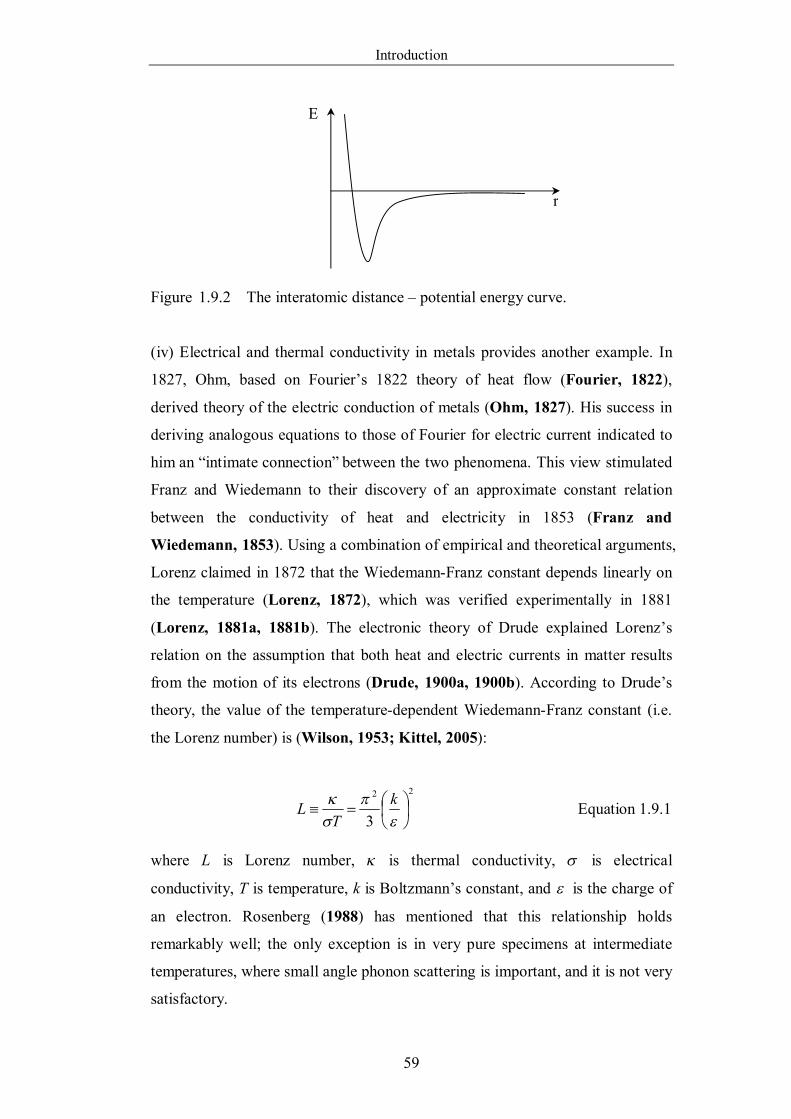
Introduction
59
Figure 1.9.2 The interatomic distance – potential energy curve.
(iv) Electrical and thermal conductivity in metals provides another example. In
1827, Ohm, based on Fourier’s 1822 theory of heat flow (Fourier, 1822),
derived theory of the electric conduction of metals (Ohm, 1827). His success in
deriving analogous equations to those of Fourier for electric current indicated to
him an “intimate connection” between the two phenomena. This view stimulated
Franz and Wiedemann to their discovery of an approximate constant relation
between the conductivity of heat and electricity in 1853 (Franz and
Wiedemann, 1853). Using a combination of empirical and theoretical arguments,
Lorenz claimed in 1872 that the Wiedemann-Franz constant depends linearly on
the temperature (Lorenz, 1872), which was verified experimentally in 1881
(Lorenz, 1881a, 1881b). The electronic theory of Drude explained Lorenz’s
relation on the assumption that both heat and electric currents in matter results
from the motion of its electrons (Drude, 1900a, 1900b). According to Drude’s
theory, the value of the temperature-dependent Wiedemann-Franz constant (i.e.
the Lorenz number) is (Wilson, 1953; Kittel, 2005):
22
3
kT
L Equation 1.9.1
where L is Lorenz number, is thermal conductivity, is electrical
conductivity, T is temperature, k is Boltzmann’s constant, and is the charge of
an electron. Rosenberg (1988) has mentioned that this relationship holds
remarkably well; the only exception is in very pure specimens at intermediate
temperatures, where small angle phonon scattering is important, and it is not very
satisfactory.
r
E
Introduction
60
However, it should be mentioned that although modern electron theory succeeds
in explaining the Wiedemann-Franz constant and the Lorenz number, closer
studies of the conduction of heat and electricity through metals showed that this
simple theory, which only considered the electrons to move freely through metals,
was unable to explain the manifold and complicated phenomena in a satisfactory
way, such as in the alkali metals where the ratio of / is extremely low
(Hornbeck, 1913). In general, the Lorenz number L, while roughly constant, is
not exactly the same for all materials; Kittel (2005) gives some values of L
ranging from L = 2.23 × 10⁻⁸ W Ω K-2 for Cu at 0 ºC to L = 3.2 × 10⁻⁸ W Ω K-2
for W at 100 ºC.
(v) Thermal expansion coefficients of materials with comparable atomic packing
vary inversely with their melting temperatures (Van Vlack, 1989). This indirect
relationship exists because the higher-melting-point materials have deeper and
therefore more symmetrical energy wells. Thus, the mean interatomic distances
of more strongly bonded materials increase less with a given change in thermal
energy.
(vi) Hardness and melting point are related because hardness is related to the
stress required to separate atoms during dislocation motion (Van Vlack, 1989).
Since larger interatomic forces of attraction imply deeper energy wells, materials
with high melting points are the harder materials, such as diamond, Al2O3 and
TiC. The correlation holds for materials with weaker bonds. However, there are
exceptions to these generalizations when more than one type of bond is present,
such as graphite and polyethylene.
(vii) The melting point and bulk modulus are related since both the melting
temperature, Tm, and the elastic modulus, E, relate to the bonding energy (Van
Vlack, 1989).
Other binary correlations exist between dielectric constant and refractive index,
toughness and hardness, an inverse correlation between dielectric loss and
dielectric strength and in porous materials, the mechanical strength and the
dielectric strength (Kishimoto et al., 1991). In functional ceramics, a dielectric
Introduction
61
which has high loss at low temperature may show ionic conduction at a higher
temperature, in oxides, a change of colour may be associated with electrical
conduction.
Ashby notes (Ashby, 1998) that some correlations have a simple theoretical basis
while others can be found by empirical methods by an appropriate search routine.
Generally, the correlations derived in a direct way from the nature of the atomic
bonding and structure are strong, such as modulus and melting point, or specific
heat and density; while those derived from properties which depend on defects in
the structure are less strong, such as strength and toughness and are weakest
when interaction with the environment is involved, such as corrosion and wear.
1.9.3 Methods for Exploring Property Correlations
Exploration of property correlations can be classified into three types: I) purely
empirical, II) partly empirical but based on some theoretical concept, III) and
purely theoretical (Reid and Sherwood, 1958). In this work, we use artificial
neural networks to explore property correlations not only for binary, but also for
ternary and more complex systems.
Examples of applying neural networks to explore property correlations include
Egolf and Jurs (1993) who used both regression and neural network techniques to
predict boiling points of organic heterocyclic compounds using the molecular
weight, dipole moment, 1st order molecule connectivity and other structure
descriptors. Michon and Hanquet (1997) used methods of quantitative structure
property relationships (QSPR) and neural networks to find non-linear relations
between chemical and rheological properties. Homer et al. (1999) developed
ANN with equilibrium physical properties and structural indicators for prediction
of viscosity, density, heat of vaporization, boiling point and Pitzer’s acentric
factor for pure organic liquid hydrocarbons at Treduced over 0.45-0.7 range.
Boozarjomehry et al. (2005) developed a set of ANNs to predict basic properties
(including critical temperature, acentric factor and molecular weight) of pure
compounds and petroleum fractions based on their normal boiling point and
liquid density at 293 K. Strechan et al. (2006) obtained correlations between the
enthalpy of vaporization, the surface tension, the molar volume and the molar
Introduction
62
mass of a substance using ANNs. Mohammadi and Richon (2007) used ANN to
predict the enthalpy of vaporization of hydrocarbons, especially heavy
hydrocarbons and petroleum fractions, from the specific gravity and normal
boiling temperatures. Karabulut and Koyuncu (2007) developed neural network
models to establish correlation of thermal conductivity with temperature and
density for propane. Recently, Giordani et al. (2009) used ANN for multiple
correlation of the mechanical properties of modified natural rubber.
The difference between these approaches and method used in this work is that all
of them needed prior knowledge to select the properties that are perceived to be
significant for the prediction. In this work, it is hoped to prepare the ground for a
wider scope which makes use of the remarkable information processing
characteristics of the computer to find the correlation between specific properties
drawn from a large number of different properties. The physical principles
behind multiple correlations found by ANNs might be deduced post facto but the
primary aim of this work is to accelerate the pace for discovering new materials
by narrowing down the compositional spaces for subsequent search either by
high throughput methods or molecular modelling.
Methods for Construction of Neural Networks
63
2.0 Methods for Construction of Neural Networks (BPANN
and PNN) For each case, there are two main works included: one is the data collection, and
the other is the neural network construction. The collected data are trained on the
constructed neural network and then this neural network is used to predict the
result based on the known parameters. In this part, the constructions of neural
network are described. The collection of data and the determination of inputs and
outputs are described separately in chapters for each case. In the work, two
different neural networks are used: one is the backpropagation neural network
(BPANN), and the other is probabilistic neural network (PNN). (Appendix 1)
2.1 Selection of Architecture of Neural Networks (BPANN)
2.1.1 Selection of the Number of Hidden Layers
It has been said that in most function approximation problems, one hidden layer
is sufficient to approximate continuous functions (Hecht-Nielsen, 1990;
Basheer, 2000); two hidden layers must generally be necessary for learning
functions with discontinuous (Masters, 1994). Any functional relationship
between inputs and outputs, as mentioned in the neural networks user’s guide
(Mathworks), can be represented by the two-hidden layers sigmoid/linear
network, if the sigmoid layer has enough neurons. As the result, a two-hidden
layer network, with tan-sigmoid transfer function in the first hidden layer and a
linear transfer function in the second hidden layer, is adopted.
2.1.2 Selection of the Number of Neurons in Hidden Layers
The size, i.e. the number of neurons, in the second hidden layer is constrained by
the number of outputs required by the problem. The outputs of the network in all
these works are always one, so there is one neuron in the second hidden layer.
The choice of number of neurons in the first hidden layer is up to the designer.
The optimum number of neurons in the first hidden layers may be a function of
(1) input/output vector size, (2) size of training and testing sub-sets and, more
importantly, (3) the problem of non-linearity (Basheer and Hajmeer, 2000).
The optimum number can be found by trial and error by placing a different
number of neurons in the first hidden layer for the same dataset.
Methods for Construction of Neural Networks
64
2.2 Selection of the Methods for Improving Generalization (BPANN)
One of the problems that occur during neural network training is called
overfitting. This happens when the error on the training set is driven to a very
small value, but the error is large when new data is presented to the network.
This is the case at which the network has memorized the training examples, but it
has not learned to generalize to new situations.
One method for improving network generalization is to use a network that is just
large enough to provide an adequate fit. The larger a network used, the more
complex the functions the network can create. If a small enough network is used,
then the network will not have enough power to overfit the date. However, it is
hard to know beforehand how large a network should be for a specific
application.
There are two other methods for improving generalization that have been
implemented in the Neural Network Toolbox: one is Bayesian Regularization
and the other is Early Stopping (Mathworks).
Bayesian Regularization: regularization involves automatically setting the
optimal performance function, which is normally chosen to be the sum of
squares of the network errors on the training set, to achieve the best
generalization. The improvement of generalization is reached by modifying
the performance function through adding a term that consists of the mean of
the sum of squares of the network weights and biases. In Bayesian
regularization framework, the weights and biases of the network are
supposed as random variables with specified distributions. Then, the
regularization parameters are estimated using statistical techniques, which
are related to the unknown variances associated with these distributions
(Mackay, 1992a; 1992b).
Early Stopping: in this technique the available data is divided into three
subsets. The first subset is the training set, which is used for computing the
gradient and updating the network weights and biases. The second subset is
the validation set. The error on the validation set is monitored during the
training process. The validation error will normally decrease during the
initial phase of training, as does the training set error. However, when the
Methods for Construction of Neural Networks
65
network begins to overfit the data, the error on the validation set will
typically begin to rise. When the validation error increases for a specified
number of iterations, the training is stopped, and the weights and biases at
the minimum of the validation error are returned.
Bayesian Regularization tends to provide better generalization performance than
Early Stopping in training function approximation networks, specially when the
size of the data set is small (Mathworks). As a result, Bayesian Regularization,
in combination with Levenberg-Marquardt training, is used for improving
generalization.
2.3 Partitioning of the Database (BPANN)
The generalizing ability of the network depends on the training database size
(Basheer and Hajmeer, 2000). Although ANN can be obtained from a training
database of any size, like other empirical models, generalization of these models
outside the model domain is adversely affected. Since ANN are required to
generalize for the unseen data, data used for training should be large enough to
cover the possible known variation in the problem domain.
The development of an ANN based on Bayesian Regularization requires
partitioning of the parent database into two sub-sets: training and testing.
Currently, there are no definitive rules for determining the required sizes of the
data sub-sets. Rules of thumb derived from experience and analogy between
ANN and statistical regression exist (Basheer and Hajmeer, 2000). Following
the method suggested by MATLAB (Mathworks), the sets are picked as equally
spaced points throughout the original data. Ratio 4:1 is selected, i.e., partitioning
the whole data set into five groups, four groups being used for training, while one
group is used for testing. The size of the training set and testing set are thus
determined, but the choice of testing set still plays a crucial role, because the
training set should include all the data belonging to the problem domain. In the
problems of materials science, it is always that the data size is small and the
problem domains are not clear, so referring to Malinov and Sha’s work (2003), a
loop program was used to redistribute the database in order to make the training
set cover the problem domain. The distribution was selected on the basis of
Methods for Construction of Neural Networks
66
regression coefficient R (R = 1 corresponds to prefect correlation) for both
training set and testing set. It is desirable that the R values for both training and
testing are as close to 1 as possible, and the difference between them are as close
to zero as possible. However, where M, the slope of the linear regression line, is
smaller than 0.9, the regression coefficient provides an unreliable criterion, and
so the selection was at the beginning based on φ = max
)(B
BR11M where
B is the intercept on ‘A’ axis and Bmax is the maximum property value. The ideal
value of this parameter is zero. In section 3.0 (i.e. Revisiting Hume-Rothery’s
Rules with Artificial Neural Networks), the distribution is selected on the basis
of φ for the testing set.
Later, considering the slope M could determine the value of intercept B, and also
in order to find the closest and highest performance for both training and testing
sets, the criterion has been improved to 2testing
2training , where =
)R1(1M , and the smallest value of is chosen. This criterion applied in
other three applied examples.
2.4 Data Normalization (BPANN)
It has been suggested by Basheer and Hajmeer (2000) that, the data should be
normalized (scaled) within a uniform range (e.g., [0 1] or [-1 1]) in order to i)
prevent larger numbers from overriding smaller ones, ii) prevent premature
saturation of the neurons of hidden layers, which would impede the learning
process.
There are two functions for scaling the inputs and targets of networks that have
been implemented in the Neural Network Toolbox:
PREMNMX: which is used to scale inputs and targets so that they fall in
the range [-1, 1];
PRESTD: which normalizes the inputs and targets so that they will have
zero mean and unity standard deviation.
As the transfer functions employed in these works are tan-sigmoid transfer
function and linear function, PREMNMX is adopted.
Methods for Construction of Neural Networks
67
In all of these four applied examples, the size of dataset is not very large.
Nevertheless, there are many situations where materials scientists would like to
benefit from ANNs in situations where the data set has inherent limitations. It has
been proved that ANN methods provide an efficient tool for experimental data
analysis even when the database size is small (Guessasma et al., 2003).
2.5 Construction of Probabilistic Neural Network (PNN)
2.5.1 Partitioning of the Database for PNN
Probabilistic neural network (PNN) is a type of radial basis network suitable for
classification problems (Specht, 1990; Vicino, 1998). As for BPANN, the
generalizing ability of PNN depends on the training database size. It is necessary
to generalize for the unseen data, so the data set used for training should be large
enough to cover the possible known variation in the problem domain. The parent
database here is partitioned into two sub-sets: training and testing. Following the
method used in construction of BPANN, as discussed previously, the sets are
picked as equally spaced points throughout the original data. The whole data set
is partitioned into five groups, four groups being used for training, and one group
is used for testing. Also due to the problem domain is not clear, a loop program is
used to redistribute the database in order to make the training set cover the
problem domain. One way that can be used to view the results is a confusion
matrix, where matrix element mij gives the number of times a sample belonging
in class Ci was assigned to Cj. As a result, the distribution was selected on the
basis of the total number of samples incorrectly placed into the class ijm
(false positives). The ideal value of ijm should be zero.
2.5.2 Choice of Spread for PNN
The spread of radial basis functions in PNN needs to be chosen. As mentioned in
MATLAB (Mathworks), if the spread is near zero, the network acts as a nearest
neighbour classifier; as spread becomes larger, the designed network takes into
account several nearby design vectors. In this work, a looped program, referring
to Malinov and Sha’s work (2003), is used in order to find the best combination
of database distribution and value of spread.
Revisiting and Development of Hume-Rothery Rules
68
3.0 Revisiting Hume-Rothery’s Rules with Artificial Neural
Networks 3.1 Special Experimental Details
3.1.1 Data Collection
Solubility Limit Collection: the solid solubility limits (at.%) for silver, copper
and gold alloys are recorded from Massalski et al. (1987), Moffatt (1994) and
ASM Handbook Vol. 3, Alloy Phase Diagrams (1992). (Listed in Appendix 2)
Physical Parameters Collection: the physical parameters, radii (Å), valences
and electrochemical factors (electronegativity) of solvent and solute atoms are
taken from Stark and Wallace (1982) and from Aylward and Findlay (1998).
The valences of elements, which were mentioned by Hume-Rothery in 1934,
follow his representation (Hume-Rothery, 1934). Radii of Al, Ga, and α-Fe
also followed Hume-Rothery’s representations (Hume-Rothery, 1961). The
structure parameter is taken from ASM Handbook Vol. 3, Alloy Phase
Diagrams (1992). (Listed in Appendix 2)
The whole dataset is used in three different ways: i) the 60 silver and copper
alloy systems, which were first mentioned by Hume-Rothery in 1934, are used
for training the neural network and testing whether the Hume-Rothery’s Rules
work in this range of alloy systems; ii) all the 408 silver and copper alloy
systems collected are used to represent the process, and then to test the effect of
introduced melting point of both solvent and solute iii) all the 566 silver, copper
and gold alloy systems are used to test the effect of melting point of both solvent
and solute, as well as for Hume-Rothery’s Rules for wider range of alloy systems.
3.1.2 Determination of Inputs and Outputs
Determination of Input Parameters
The network input parameters are the physical parameters including i) atomic
size parameter, ii) valence parameter, iii) electrochemical parameter, i.e.
electronegativity, and iv) structure parameter of solvent and solute atoms, which
were not mentioned in 1934 by Hume-Rothery, but were introduced in 1948
(Axon and Hume-Rothery, 1948) concerning the detailed examination of
Vegard’s law (Vegard, 1921) in the case of metallic solid solutions.
Revisiting and Development of Hume-Rothery Rules
69
Three different expressions of these parameters are used:
1. The raw data that Hume-Rothery used. Details are discussed below.
2. The original collected values for each parameter of solvent and solute atoms.
3. The original collected parameters are converted into functionalized values
before putting them into the networks:
a) For Size Factor: The difference between the atomic diameters of solvent
and solute atoms divided by the diameter of the solvent atom is used.
b) For Valence Factor: These are integers and the original values are used,
leaving the neural network to decide the relations between valence of
solvents and solutes.
c) For Electrochemical Factor: The difference between that of the solvent and
solute atoms is used.
d) For Structure Parameter: The expressions of the structures can be put in
terms of numbers 1-14 for the Bravais lattices, but this revealed little effect
of structure. They can also be expressed in three sets of numbers
representing primitive cell dimensions, angles and systems. This allows
some similarities to be explored. The three sets are i) unit cell length (a=b=c;
a=b≠c; a≠b≠c), ii) axes angles (α=β=γ=90º; α=β=90º, γ=120º; α=β=γ≠90º;
α=γ=90º≠β; α≠β≠γ≠90º) and iii) crystal system (simple; base-centred; face-
centred; body-centred).
Later, we were curious if more rules are needed to extend Hume-Rothery’s
principle into quantitative solubility prediction of a wider range of alloy systems
using ANN. As the result, one new parameter was introduced:
e) Melting point (Tm): It is well known that the solubility of many solids
depends on temperature. As a result, it is reasonable to consider improving
the performance of prediction by introducing temperature as a parameter.
The melting temperature (Tm, in the unit of ºC), above which two metals are
miscible in any proportions, was proposed as an additional parameter.
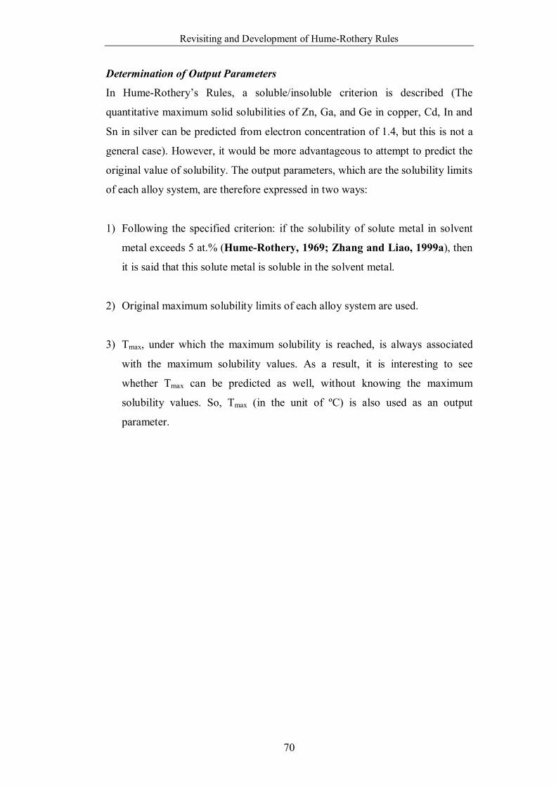
Revisiting and Development of Hume-Rothery Rules
70
Determination of Output Parameters
In Hume-Rothery’s Rules, a soluble/insoluble criterion is described (The
quantitative maximum solid solubilities of Zn, Ga, and Ge in copper, Cd, In and
Sn in silver can be predicted from electron concentration of 1.4, but this is not a
general case). However, it would be more advantageous to attempt to predict the
original value of solubility. The output parameters, which are the solubility limits
of each alloy system, are therefore expressed in two ways:
1) Following the specified criterion: if the solubility of solute metal in solvent
metal exceeds 5 at.% (Hume-Rothery, 1969; Zhang and Liao, 1999a), then
it is said that this solute metal is soluble in the solvent metal.
2) Original maximum solubility limits of each alloy system are used.
3) Tmax, under which the maximum solubility is reached, is always associated
with the maximum solubility values. As a result, it is interesting to see
whether Tmax can be predicted as well, without knowing the maximum
solubility values. So, Tmax (in the unit of ºC) is also used as an output
parameter.
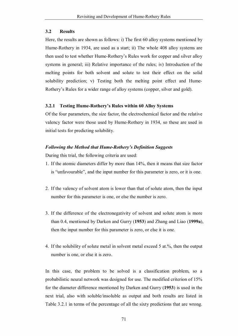
Revisiting and Development of Hume-Rothery Rules
71
3.2 Results
Here, the results are shown as follows: i) The first 60 alloy systems mentioned by
Hume-Rothery in 1934, are used as a start; ii) The whole 408 alloy systems are
then used to test whether Hume-Rothery’s Rules work for copper and silver alloy
systems in general; iii) Relative importance of the rules; iv) Introduction of the
melting points for both solvent and solute to test their effect on the solid
solubility prediction; v) Testing both the melting point effect and Hume-
Rothery’s Rules for a wider range of alloy systems (copper, silver and gold).
3.2.1 Testing Hume-Rothery’s Rules within 60 Alloy Systems
Of the four parameters, the size factor, the electrochemical factor and the relative
valency factor were those used by Hume-Rothery in 1934, so these are used in
initial tests for predicting solubility.
Following the Method that Hume-Rothery’s Definition Suggests
During this trial, the following criteria are used:
1. If the atomic diameters differ by more than 14%, then it means that size factor
is “unfavourable”, and the input number for this parameter is zero, or it is one.
2. If the valency of solvent atom is lower than that of solute atom, then the input
number for this parameter is one, or else the number is zero.
3. If the difference of the electronegativity of solvent and solute atom is more
than 0.4, mentioned by Darken and Gurry (1953) and Zhang and Liao (1999a),
then the input number for this parameter is zero, or else it is one.
4. If the solubility of solute metal in solvent metal exceed 5 at.%, then the output
number is one, or else it is zero.
In this case, the problem to be solved is a classification problem, so a
probabilistic neural network was designed for use. The modified criterion of 15%
for the diameter difference mentioned by Darken and Gurry (1953) is used in the
next trial, also with soluble/insoluble as output and both results are listed in
Table 3.2.1 in terms of the percentage of all the sixty predictions that are wrong.
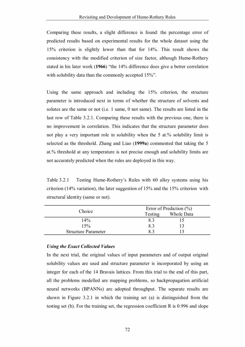
Revisiting and Development of Hume-Rothery Rules
72
Comparing these results, a slight difference is found: the percentage error of
predicted results based on experimental results for the whole dataset using the
15% criterion is slightly lower than that for 14%. This result shows the
consistency with the modified criterion of size factor, although Hume-Rothery
stated in his later work (1966) “the 14% difference does give a better correlation
with solubility data than the commonly accepted 15%”.
Using the same approach and including the 15% criterion, the structure
parameter is introduced next in terms of whether the structure of solvents and
solutes are the same or not (i.e. 1 same, 0 not same). The results are listed in the
last row of Table 3.2.1. Comparing these results with the previous one, there is
no improvement in correlation. This indicates that the structure parameter does
not play a very important role in solubility when the 5 at.% solubility limit is
selected as the threshold. Zhang and Liao (1999a) commented that taking the 5
at.% threshold at any temperature is not precise enough and solubility limits are
not accurately predicted when the rules are deployed in this way.
Table 3.2.1 Testing Hume-Rothery’s Rules with 60 alloy systems using his
criterion (14% variation), the later suggestion of 15% and the 15% criterion with
structural identity (same or not).
Choice Error of Prediction (%) Testing Whole Data
14% 8.3 15 15% 8.3 13
Structure Parameter 8.3 13
Using the Exact Collected Values
In the next trial, the original values of input parameters and of output original
solubility values are used and structure parameter is incorporated by using an
integer for each of the 14 Bravais lattices. From this trial to the end of this part,
all the problems modelled are mapping problems, so backpropagation artificial
neural networks (BPANNs) are adopted throughput. The separate results are
shown in Figure 3.2.1 in which the training set (a) is distinguished from the
testing set (b). For the training set, the regression coefficient R is 0.996 and slope
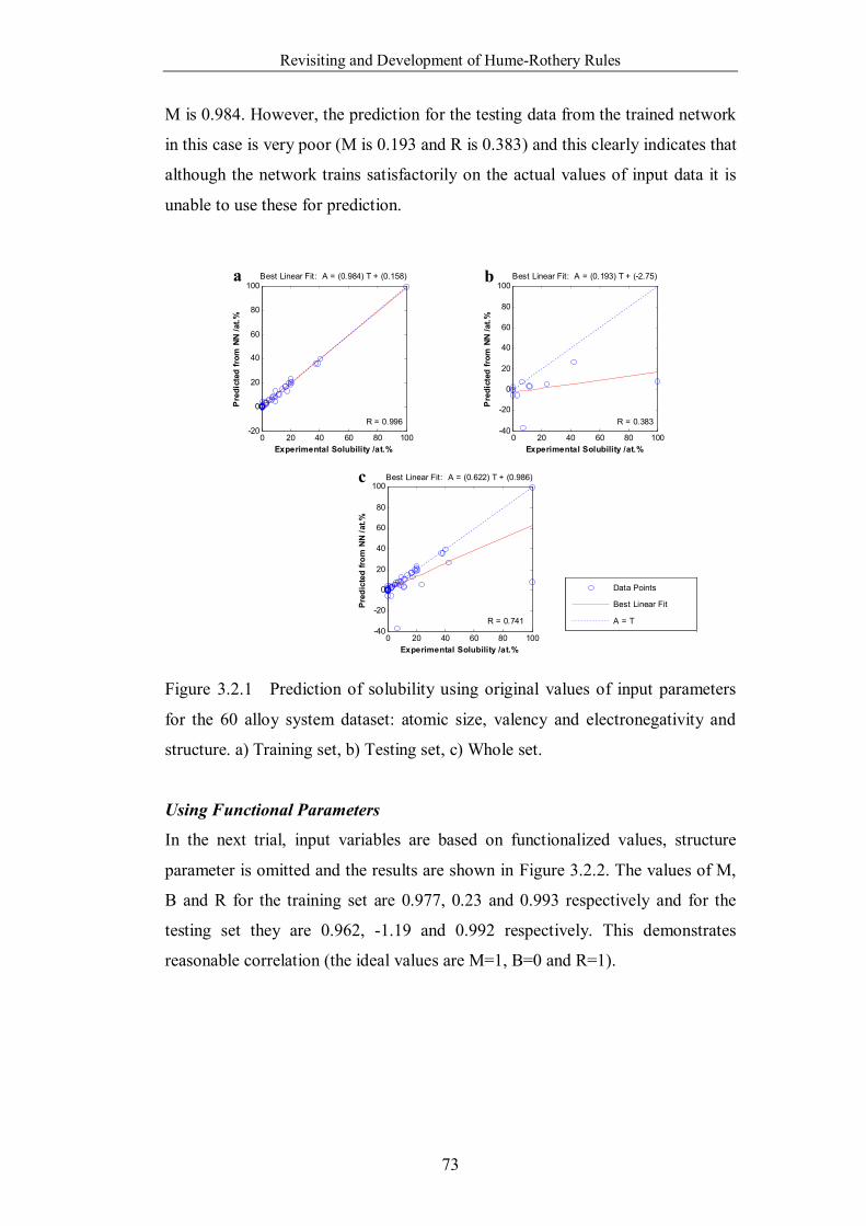
Revisiting and Development of Hume-Rothery Rules
73
M is 0.984. However, the prediction for the testing data from the trained network
in this case is very poor (M is 0.193 and R is 0.383) and this clearly indicates that
although the network trains satisfactorily on the actual values of input data it is
unable to use these for prediction.
0 20 40 60 80 100-20
0
20
40
60
80
100
Experimental Solubility /at.%
Pre
dict
ed fr
om N
N /a
t.%
Best Linear Fit: A = (0.984) T + (0.158)
R = 0.996
0 20 40 60 80 100-40
-20
0
20
40
60
80
100
Experimental Solubility /at.%
Pre
dict
ed fr
om N
N /a
t.%
Best Linear Fit: A = (0.193) T + (-2.75)
R = 0.383
0 20 40 60 80 100-40
-20
0
20
40
60
80
100
Experimental Solubility /at.%
Pred
icte
d fro
m N
N /a
t.%
Best Linear Fit: A = (0.622) T + (0.986)
R = 0.741
Data Points
Best Linear Fit
A = T
Figure 3.2.1 Prediction of solubility using original values of input parameters
for the 60 alloy system dataset: atomic size, valency and electronegativity and
structure. a) Training set, b) Testing set, c) Whole set.
Using Functional Parameters
In the next trial, input variables are based on functionalized values, structure
parameter is omitted and the results are shown in Figure 3.2.2. The values of M,
B and R for the training set are 0.977, 0.23 and 0.993 respectively and for the
testing set they are 0.962, -1.19 and 0.992 respectively. This demonstrates
reasonable correlation (the ideal values are M=1, B=0 and R=1).
a b
c
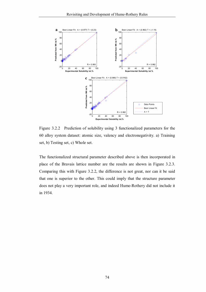
Revisiting and Development of Hume-Rothery Rules
74
0 20 40 60 80 100-20
0
20
40
60
80
100
Experimental Solubility /at.%
Pre
dict
ed fr
om N
N /a
t.%
Best Linear Fit: A = (0.977) T + (0.23)
R = 0.993
0 20 40 60 80 100-20
0
20
40
60
80
100
Experimental Solubility /at.%
Pre
dict
ed fr
om N
N /a
t.%
Best Linear Fit: A = (0.962) T + (-1.19)
R = 0.992
0 20 40 60 80 100-20
0
20
40
60
80
100
Experimental Solubility /at.%
Pre
dict
ed fr
om N
N /a
t.%
Best Linear Fit: A = (0.966) T + (0.0162)
R = 0.992
Data Points
Best Linear Fit
A = T
Figure 3.2.2 Prediction of solubility using 3 functionalized parameters for the
60 alloy system dataset: atomic size, valency and electronegativity. a) Training
set, b) Testing set, c) Whole set.
The functionalized structural parameter described above is then incorporated in
place of the Bravais lattice number are the results are shown in Figure 3.2.3.
Comparing this with Figure 3.2.2, the difference is not great, nor can it be said
that one is superior to the other. This could imply that the structure parameter
does not play a very important role, and indeed Hume-Rothery did not include it
in 1934.
a b
c
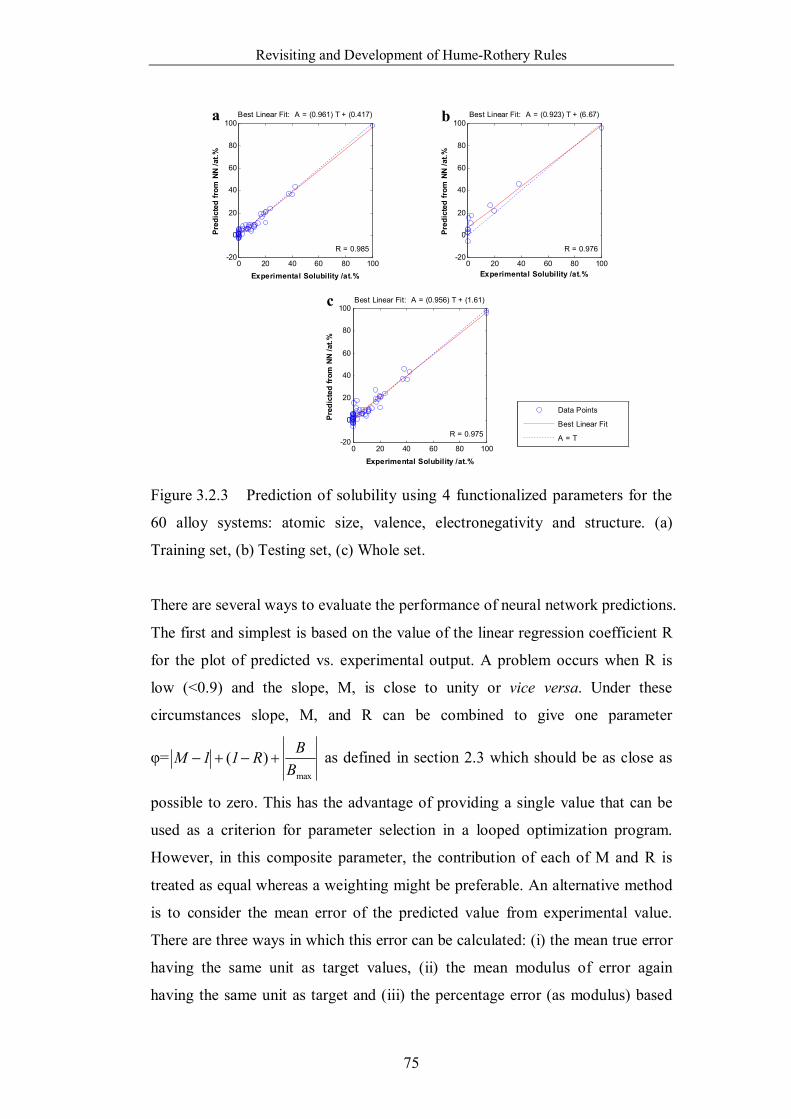
Revisiting and Development of Hume-Rothery Rules
75
0 20 40 60 80 100-20
0
20
40
60
80
100
Experimental Solubility /at.%
Pred
icte
d fr
om N
N /a
t.%
Best Linear Fit: A = (0.961) T + (0.417)
R = 0.985
0 20 40 60 80 100-20
0
20
40
60
80
100
Experimental Solubility /at.%
Pred
icte
d fr
om N
N /a
t.%
Best Linear Fit: A = (0.923) T + (6.67)
R = 0.976
0 20 40 60 80 100-20
0
20
40
60
80
100
Experimental Solubility /at.%
Pred
icte
d fr
om N
N /a
t.%
Best Linear Fit: A = (0.956) T + (1.61)
R = 0.975
Data Points
Best Linear Fit
A = T
Figure 3.2.3 Prediction of solubility using 4 functionalized parameters for the
60 alloy systems: atomic size, valence, electronegativity and structure. (a)
Training set, (b) Testing set, (c) Whole set.
There are several ways to evaluate the performance of neural network predictions.
The first and simplest is based on the value of the linear regression coefficient R
for the plot of predicted vs. experimental output. A problem occurs when R is
low (<0.9) and the slope, M, is close to unity or vice versa. Under these
circumstances slope, M, and R can be combined to give one parameter
φ=max
)(B
BR11M as defined in section 2.3 which should be as close as
possible to zero. This has the advantage of providing a single value that can be
used as a criterion for parameter selection in a looped optimization program.
However, in this composite parameter, the contribution of each of M and R is
treated as equal whereas a weighting might be preferable. An alternative method
is to consider the mean error of the predicted value from experimental value.
There are three ways in which this error can be calculated: (i) the mean true error
having the same unit as target values, (ii) the mean modulus of error again
having the same unit as target and (iii) the percentage error (as modulus) based
a b
c
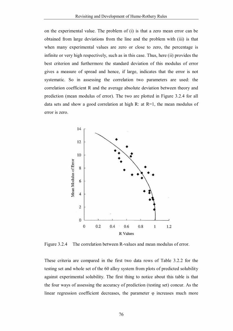
Revisiting and Development of Hume-Rothery Rules
76
on the experimental value. The problem of (i) is that a zero mean error can be
obtained from large deviations from the line and the problem with (iii) is that
when many experimental values are zero or close to zero, the percentage is
infinite or very high respectively, such as in this case. Thus, here (ii) provides the
best criterion and furthermore the standard deviation of this modulus of error
gives a measure of spread and hence, if large, indicates that the error is not
systematic. So in assessing the correlation two parameters are used: the
correlation coefficient R and the average absolute deviation between theory and
prediction (mean modulus of error). The two are plotted in Figure 3.2.4 for all
data sets and show a good correlation at high R: at R=1, the mean modulus of
error is zero.
Figure 3.2.4 The correlation between R-values and mean modulus of error.
These criteria are compared in the first two data rows of Table 3.2.2 for the
testing set and whole set of the 60 alloy system from plots of predicted solubility
against experimental solubility. The first thing to notice about this table is that
the four ways of assessing the accuracy of prediction (testing set) concur. As the
linear regression coefficient decreases, the parameter φ increases much more
Revisiting and Development of Hume-Rothery Rules
77
dramatically and can be regarded as a more sensitive indicator for this reason.
Also a simple calculation of the mean deviation of the predicted values from the
best fit line (mean modulus of error) gives an estimate of the accuracy of
prediction. This follows the trend of increasing φ and reduced R. The standard
deviation for this error is an indicator that the error is random rather than
systematic and if so, the standard deviation is expected to increase with the mean
as it, in fact, does. The ratio of standard deviation of error to mean error is, in all
but one case, greater than unity. This trends in the assessment criteria are
consistent for both the testing set and the whole set.
The best predictive results for the network are obtained by using the
functionalized values of atomic size, valence and electronegativity to predict
original values of solubility for the 60-alloy dataset used by Hume-Rothery
himself and the data are plotted in Figure 3.2.2. Inclusion of the structural factor
using the parameter described above weakens the predictive power of the
network (Figure 3.2.3). The reason for this slightly counter-intuitive finding is
that crystallographic compatibility is likely to become more important at higher
solubility levels, being essential for continuous solubility. However, the majority
of data are at the low solubility end where substitutional atoms are at low co-
ordination number. Another reason is that the number used to represent structure
actually conceals crystallographic similarities as discussed in more detail below
and there is not enough training data for the network to establish these
similarities by itself. The structure parameter is used to assess the criterion for
solubility that “the same crystal structure for the two elements favours a wide
solubility range” (Wyatt and Dew-Hughes, 1974). This makes it a kind of
classification problem, not completely the same as a mapping problem and it
could be argued that including it in this type of network is inappropriate.
3.2.2 Testing Hume-Rothery’s Rules within 408 Alloy Systems
From the results for the 60 alloy systems, it is clear that using the 3
functionalized values of parameters provides better results, so the same approach
is adopted for testing the 408 alloy systems. This represents a nearly exhaustive
set of known silver and copper alloys. The results, shown in the last row of Table
3.2.2 and plotted in Figure 3.2.5, use the same format of inputs as those used for
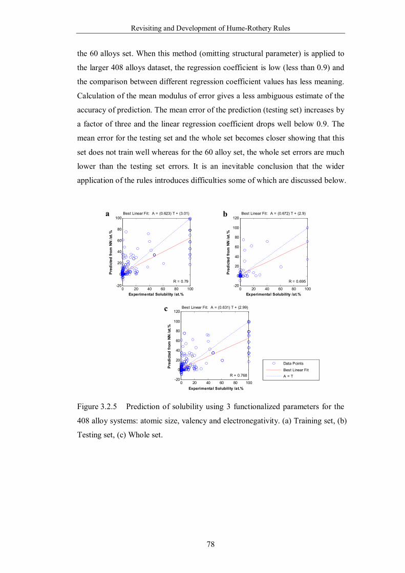
Revisiting and Development of Hume-Rothery Rules
78
the 60 alloys set. When this method (omitting structural parameter) is applied to
the larger 408 alloys dataset, the regression coefficient is low (less than 0.9) and
the comparison between different regression coefficient values has less meaning.
Calculation of the mean modulus of error gives a less ambiguous estimate of the
accuracy of prediction. The mean error of the prediction (testing set) increases by
a factor of three and the linear regression coefficient drops well below 0.9. The
mean error for the testing set and the whole set becomes closer showing that this
set does not train well whereas for the 60 alloy set, the whole set errors are much
lower than the testing set errors. It is an inevitable conclusion that the wider
application of the rules introduces difficulties some of which are discussed below.
0 20 40 60 80 100-20
0
20
40
60
80
100
Experimental Solubility /at.%
Pred
icte
d fro
m N
N /a
t.%
Best Linear Fit: A = (0.623) T + (3.01)
R = 0.79
0 20 40 60 80 100-20
0
20
40
60
80
100
120
Experimental Solubility /at.%
Pred
icte
d fro
m N
N /a
t.%
Best Linear Fit: A = (0.672) T + (2.9)
R = 0.695
0 20 40 60 80 100-20
0
20
40
60
80
100
120
Experimental Solubility /at.%
Pre
dict
ed fr
om N
N /a
t.%
Best Linear Fit: A = (0.631) T + (2.99)
R = 0.768
Data Points
Best Linear FitA = T
Figure 3.2.5 Prediction of solubility using 3 functionalized parameters for the
408 alloy systems: atomic size, valency and electronegativity. (a) Training set, (b)
Testing set, (c) Whole set.
a b
c
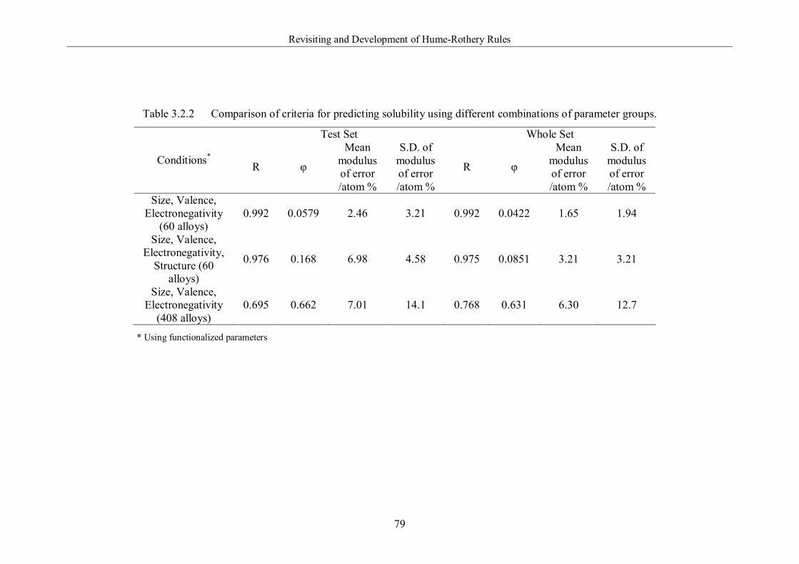
Revisiting and Development of Hume-Rothery Rules
79
Table 3.2.2 Comparison of criteria for predicting solubility using different combinations of parameter groups.
Test Set Whole Set
Conditions* R φ
Mean modulus of error /atom %
S.D. of modulus of error /atom %
R φ
Mean modulus of error /atom %
S.D. of modulus of error /atom %
Size, Valence, Electronegativity
(60 alloys) 0.992 0.0579 2.46 3.21 0.992 0.0422 1.65 1.94
Size, Valence, Electronegativity,
Structure (60 alloys)
0.976 0.168 6.98 4.58 0.975 0.0851 3.21 3.21
Size, Valence, Electronegativity
(408 alloys) 0.695 0.662 7.01 14.1 0.768 0.631 6.30 12.7
* Using functionalized parameters
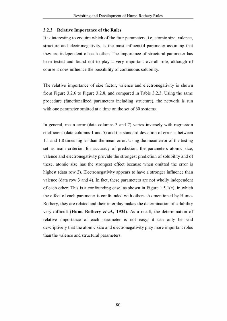
Revisiting and Development of Hume-Rothery Rules
80
3.2.3 Relative Importance of the Rules
It is interesting to enquire which of the four parameters, i.e. atomic size, valence,
structure and electronegativity, is the most influential parameter assuming that
they are independent of each other. The importance of structural parameter has
been tested and found not to play a very important overall role, although of
course it does influence the possibility of continuous solubility.
The relative importance of size factor, valence and electronegativity is shown
from Figure 3.2.6 to Figure 3.2.8, and compared in Table 3.2.3. Using the same
procedure (functionalized parameters including structure), the network is run
with one parameter omitted at a time on the set of 60 systems.
In general, mean error (data columns 3 and 7) varies inversely with regression
coefficient (data columns 1 and 5) and the standard deviation of error is between
1.1 and 1.8 times higher than the mean error. Using the mean error of the testing
set as main criterion for accuracy of prediction, the parameters atomic size,
valence and electronegativity provide the strongest prediction of solubility and of
these, atomic size has the strongest effect because when omitted the error is
highest (data row 2). Electronegativity appears to have a stronger influence than
valence (data row 3 and 4). In fact, these parameters are not wholly independent
of each other. This is a confounding case, as shown in Figure 1.5.1(c), in which
the effect of each parameter is confounded with others. As mentioned by Hume-
Rothery, they are related and their interplay makes the determination of solubility
very difficult (Hume-Rothery et al., 1934). As a result, the determination of
relative importance of each parameter is not easy; it can only be said
descriptively that the atomic size and electronegativity play more important roles
than the valence and structural parameters.
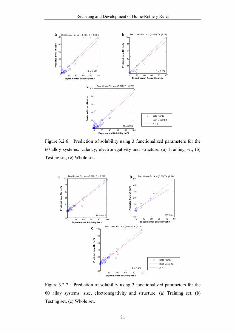
Revisiting and Development of Hume-Rothery Rules
81
0 20 40 60 80 1000
20
40
60
80
100
Experimental Solubility /at.%
Pred
icte
d fro
m N
N /a
t.%
Best Linear Fit: A = (0.906) T + (0.904)
R = 0.958
0 20 40 60 80 1000
20
40
60
80
100
Experimental Solubility /at.%
Pre
dict
ed fr
om N
N /a
t.%
Best Linear Fit: A = (0.856) T + (3.13)
R = 0.867
0 20 40 60 80 1000
20
40
60
80
100
Experimental Solubility /at.%
Pred
icte
d fro
m N
N /a
t.%Best Linear Fit: A = (0.892) T + (1.33)
R = 0.924
Data Points
Best Linear Fit
A = T
Figure 3.2.6 Prediction of solubility using 3 functionalized parameters for the
60 alloy systems: valency, electronegativity and structure. (a) Training set, (b)
Testing set, (c) Whole set.
0 20 40 60 80 100-20
0
20
40
60
80
100
Experimental Solubility /at.%
Pre
dict
ed fr
om N
N /a
t.%
Best Linear Fit: A = (0.917) T + (0.982)
R = 0.972
0 10 20 30 40 50-10
0
10
20
30
40
50
Experimental Solubility /at.%
Pred
icte
d fr
om N
N /a
t.%
Best Linear Fit: A = (0.73) T + (2.54)
R = 0.93
0 20 40 60 80 100-20
0
20
40
60
80
100
Experimental Solubility /at.%
Pred
icte
d fr
om N
N /a
t.%
Best Linear Fit: A = (0.901) T + (1.11)
R = 0.968
Data Points
Best Linear Fit
A = T
Figure 3.2.7 Prediction of solubility using 3 functionalized parameters for the
60 alloy systems: size, electronegativity and structure. (a) Training set, (b)
Testing set, (c) Whole set.
a b
c
a b
c
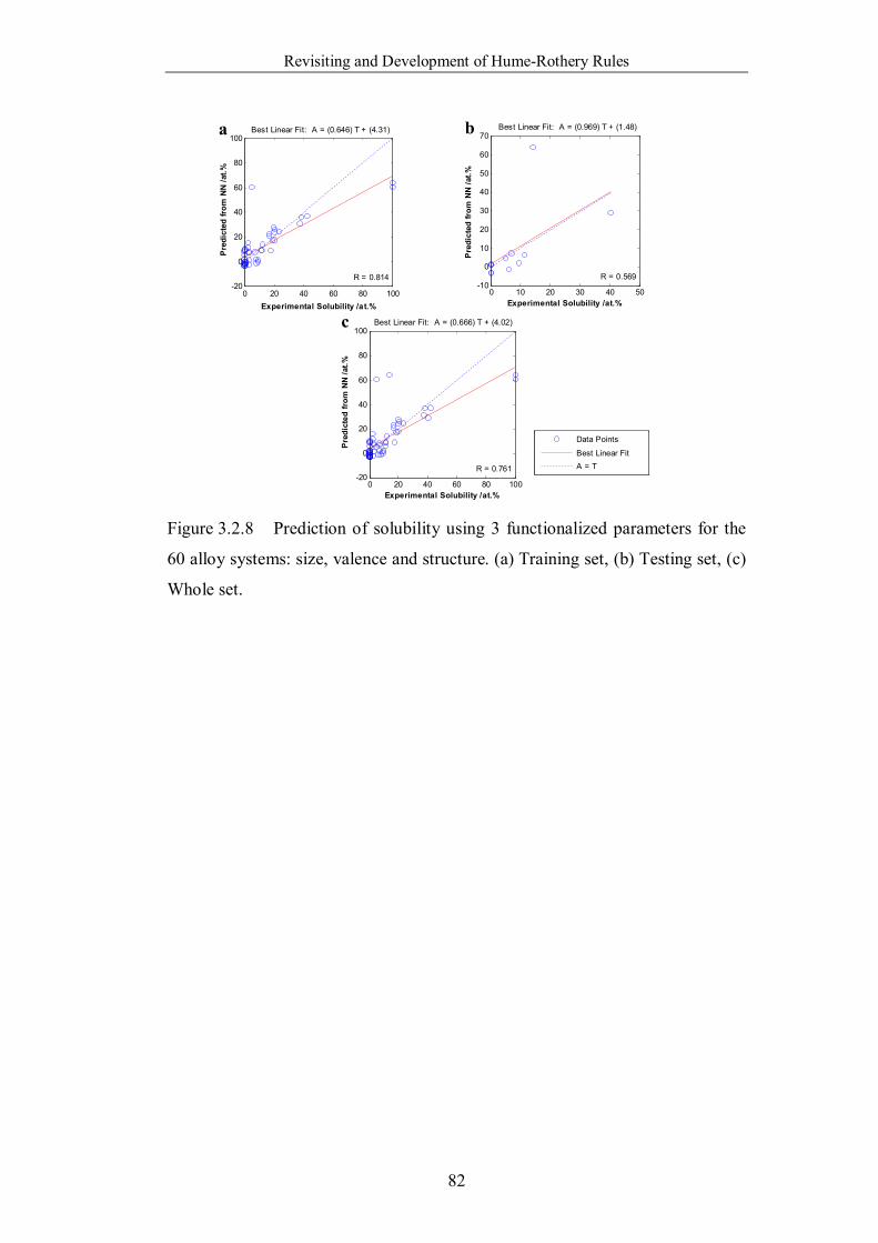
Revisiting and Development of Hume-Rothery Rules
82
0 20 40 60 80 100-20
0
20
40
60
80
100
Experimental Solubility /at.%
Pre
dict
ed fr
om N
N /a
t.%
Best Linear Fit: A = (0.646) T + (4.31)
R = 0.814
0 10 20 30 40 50-10
0
10
20
30
40
50
60
70
Experimental Solubility /at.%
Pre
dict
ed fr
om N
N /a
t.%
Best Linear Fit: A = (0.969) T + (1.48)
R = 0.569
0 20 40 60 80 100-20
0
20
40
60
80
100
Experimental Solubility /at.%
Pre
dict
ed fr
om N
N /a
t.%
Best Linear Fit: A = (0.666) T + (4.02)
R = 0.761
Data Points
Best Linear FitA = T
Figure 3.2.8 Prediction of solubility using 3 functionalized parameters for the
60 alloy systems: size, valence and structure. (a) Training set, (b) Testing set, (c)
Whole set.
a b
c
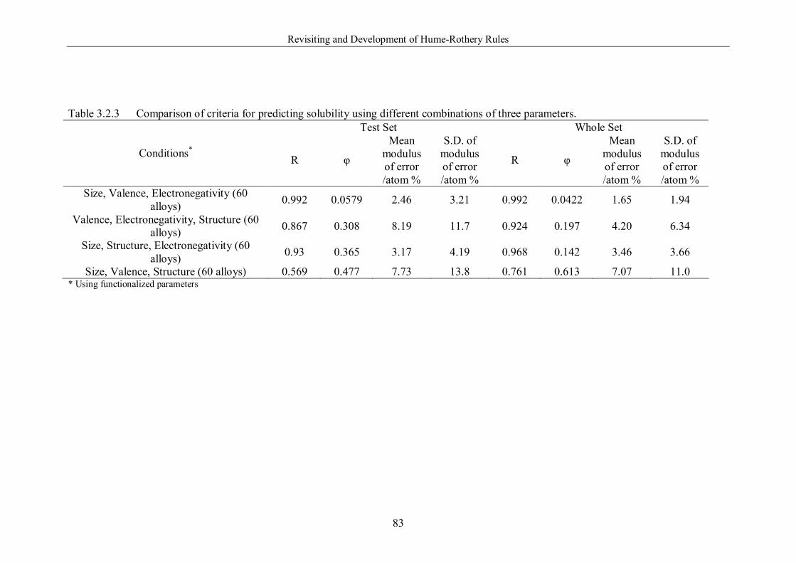
Revisiting and Development of Hume-Rothery Rules
83
Table 3.2.3 Comparison of criteria for predicting solubility using different combinations of three parameters. Test Set Whole Set
Conditions* R φ
Mean modulus of error /atom %
S.D. of modulus of error /atom %
R φ
Mean modulus of error /atom %
S.D. of modulus of error /atom %
Size, Valence, Electronegativity (60 alloys) 0.992 0.0579 2.46 3.21 0.992 0.0422 1.65 1.94
Valence, Electronegativity, Structure (60 alloys) 0.867 0.308 8.19 11.7 0.924 0.197 4.20 6.34
Size, Structure, Electronegativity (60 alloys) 0.93 0.365 3.17 4.19 0.968 0.142 3.46 3.66
Size, Valence, Structure (60 alloys) 0.569 0.477 7.73 13.8 0.761 0.613 7.07 11.0 * Using functionalized parameters
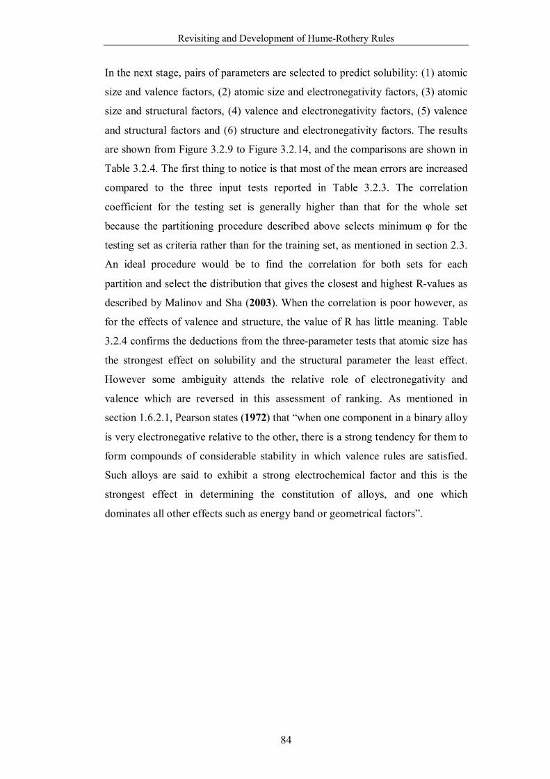
Revisiting and Development of Hume-Rothery Rules
84
In the next stage, pairs of parameters are selected to predict solubility: (1) atomic
size and valence factors, (2) atomic size and electronegativity factors, (3) atomic
size and structural factors, (4) valence and electronegativity factors, (5) valence
and structural factors and (6) structure and electronegativity factors. The results
are shown from Figure 3.2.9 to Figure 3.2.14, and the comparisons are shown in
Table 3.2.4. The first thing to notice is that most of the mean errors are increased
compared to the three input tests reported in Table 3.2.3. The correlation
coefficient for the testing set is generally higher than that for the whole set
because the partitioning procedure described above selects minimum φ for the
testing set as criteria rather than for the training set, as mentioned in section 2.3.
An ideal procedure would be to find the correlation for both sets for each
partition and select the distribution that gives the closest and highest R-values as
described by Malinov and Sha (2003). When the correlation is poor however, as
for the effects of valence and structure, the value of R has little meaning. Table
3.2.4 confirms the deductions from the three-parameter tests that atomic size has
the strongest effect on solubility and the structural parameter the least effect.
However some ambiguity attends the relative role of electronegativity and
valence which are reversed in this assessment of ranking. As mentioned in
section 1.6.2.1, Pearson states (1972) that “when one component in a binary alloy
is very electronegative relative to the other, there is a strong tendency for them to
form compounds of considerable stability in which valence rules are satisfied.
Such alloys are said to exhibit a strong electrochemical factor and this is the
strongest effect in determining the constitution of alloys, and one which
dominates all other effects such as energy band or geometrical factors”.
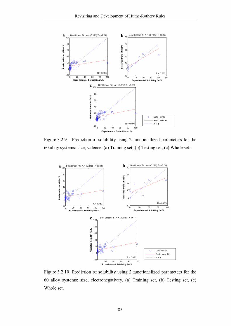
Revisiting and Development of Hume-Rothery Rules
85
0 20 40 60 80 100-20
0
20
40
60
80
100
Experimental Solubility /at.%
Pre
dict
ed fr
om N
N /a
t.%
Best Linear Fit: A = (0.195) T + (9.54)
R = 0.455
0 10 20 30 40 50-10
0
10
20
30
40
50
Experimental Solubility /at.%
Pre
eict
ed fr
om N
N /a
t.%
Best Linear Fit: A = (0.717) T + (3.86)
R = 0.852
0 20 40 60 80 100-20
0
20
40
60
80
100
Experimental Solubility /at.%
Pre
dict
ed fr
om N
N /a
t.%
Best Linear Fit: A = (0.234) T + (9.08)
R = 0.496
Data Points
Best Linear FitA = T
Figure 3.2.9 Prediction of solubility using 2 functionalized parameters for the
60 alloy systems: size, valence. (a) Training set, (b) Testing set, (c) Whole set.
0 20 40 60 80 100-20
0
20
40
60
80
100
Experimental Solubility /at.%
Pre
dict
ed fr
om N
N /a
t.%
Best Linear Fit: A = (0.218) T + (9.23)
R = 0.482
0 10 20 30 40-10
0
10
20
30
40
Experimental Solubility /at.%
Pred
icte
d fr
om N
N /a
t.%
Best Linear Fit: A = (0.526) T + (6.54)
R = 0.679
0 20 40 60 80 100-20
0
20
40
60
80
100
Experimental Solubility /at.%
Pre
dict
ed fr
om N
N /a
t.%
Best Linear Fit: A = (0.238) T + (9.11)
R = 0.495
Data Points
Best Linear FitA = T
Figure 3.2.10 Prediction of solubility using 2 functionalized parameters for the
60 alloy systems: size, electronegativity. (a) Training set, (b) Testing set, (c)
Whole set.
a b
c
a b
c
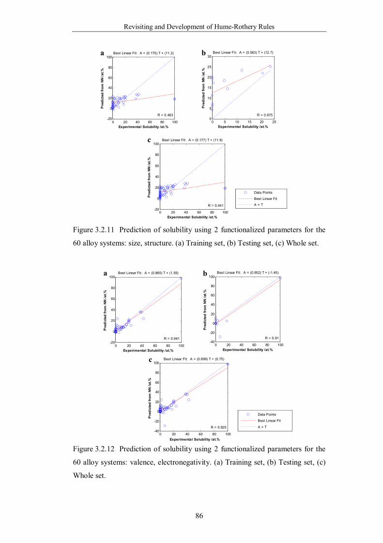
Revisiting and Development of Hume-Rothery Rules
86
0 20 40 60 80 100-20
0
20
40
60
80
100
Experimental Solubility /at.%
Pre
dict
ed fr
om N
N /a
t.%
Best Linear Fit: A = (0.175) T + (11.2)
R = 0.463
0 5 10 15 20 250
5
10
15
20
25
30
Experimental Solubility /at.%
Pre
dict
ed fr
om N
N /a
t.%
Best Linear Fit: A = (0.563) T + (12.7)
R = 0.675
0 20 40 60 80 100-20
0
20
40
60
80
100
Experimental Solubility /at.%
Pre
dict
ed fr
om N
N /a
t.%
Best Linear Fit: A = (0.177) T + (11.9)
R = 0.441
Data Points
Best Linear Fit
A = T
Figure 3.2.11 Prediction of solubility using 2 functionalized parameters for the
60 alloy systems: size, structure. (a) Training set, (b) Testing set, (c) Whole set.
0 20 40 60 80 100-20
0
20
40
60
80
100
Experimental Solubility /at.%
Pre
dict
ed fr
om N
N /a
t.%
Best Linear Fit: A = (0.865) T + (1.55)
R = 0.941
0 20 40 60 80 100-40
-20
0
20
40
60
80
100
Experimental Solubility /at.%
Pre
dict
ed fr
om N
N /a
t.%
Best Linear Fit: A = (0.952) T + (-1.45)
R = 0.91
0 20 40 60 80 100-40
-20
0
20
40
60
80
100
Experimental Solubility /at.%
Pre
dict
ed fr
om N
N /a
t.%
Best Linear Fit: A = (0.899) T + (0.75)
R = 0.925
Data Points
Best Linear Fit
A = T
Figure 3.2.12 Prediction of solubility using 2 functionalized parameters for the
60 alloy systems: valence, electronegativity. (a) Training set, (b) Testing set, (c)
Whole set.
a b
c
a b
c
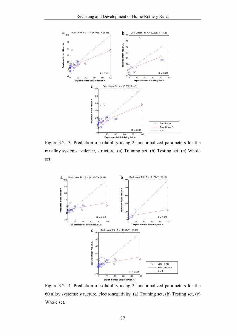
Revisiting and Development of Hume-Rothery Rules
87
0 20 40 60 80 100-20
0
20
40
60
80
100
Experimental Solubility /at.%
Pred
icte
d fro
m N
N /a
t.%
Best Linear Fit: A = (0.496) T + (5.86)
R = 0.723
0 10 20 30 40 50-10
0
10
20
30
40
50
60
Experimental Solubility /at.%
Pred
icte
d fro
m N
N /a
t.%
Best Linear Fit: A = (0.535) T + (1.5)
R = 0.459
0 20 40 60 80 100-20
0
20
40
60
80
100
Experimental Solubility /at.%
Pre
dict
ed fr
om N
N /a
t.%
Best Linear Fit: A = (0.502) T + (5)
R = 0.662
Data Points
Best Linear FitA = T
Figure 3.2.13 Prediction of solubility using 2 functionalized parameters for the
60 alloy systems: valence, structure. (a) Training set, (b) Testing set, (c) Whole
set.
0 20 40 60 80 100-20
0
20
40
60
80
100
Experimental Solubility /at.%
Pred
icte
d fr
om N
N /a
t.%
Best Linear Fit: A = (0.237) T + (8.64)
R = 0.512
0 20 40 60 80 1000
20
40
60
80
100
Experimental Solubility /at.%
Pre
dict
ed fr
om N
N /a
t.%
Best Linear Fit: A = (0.176) T + (8.17)
R = 0.607
0 20 40 60 80 100-20
0
20
40
60
80
100
Experimental Solubility /at.%
Pre
dict
ed fr
om N
N /a
t.%
Best Linear Fit: A = (0.213) T + (8.65)
R = 0.524
Data Points
Best Linear FitA = T
Figure 3.2.14 Prediction of solubility using 2 functionalized parameters for the
60 alloy systems: structure, electronegativity. (a) Training set, (b) Testing set, (c)
Whole set.
a b
c
a b
c
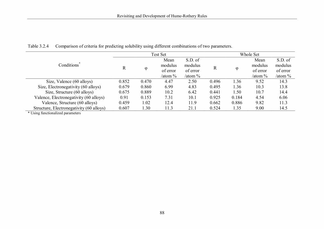
Revisiting and Development of Hume-Rothery Rules
88
Table 3.2.4 Comparison of criteria for predicting solubility using different combinations of two parameters.
Test Set Whole Set
Conditions* R φ
Mean modulus of error /atom %
S.D. of modulus of error /atom %
R φ
Mean modulus of error /atom %
S.D. of modulus of error /atom %
Size, Valence (60 alloys) 0.852 0.470 4.47 2.50 0.496 1.36 9.52 14.3 Size, Electronegativity (60 alloys) 0.679 0.860 6.99 4.83 0.495 1.36 10.3 13.8
Size, Structure (60 alloys) 0.675 0.889 10.2 6.42 0.441 1.50 10.7 14.4 Valence, Electronegativity (60 alloys) 0.91 0.153 7.31 10.1 0.925 0.184 4.54 6.06
Valence, Structure (60 alloys) 0.459 1.02 12.4 11.9 0.662 0.886 9.82 11.3 Structure, Electronegativity (60 alloys) 0.607 1.30 11.3 21.1 0.524 1.35 9.00 14.5
* Using functionalized parameters
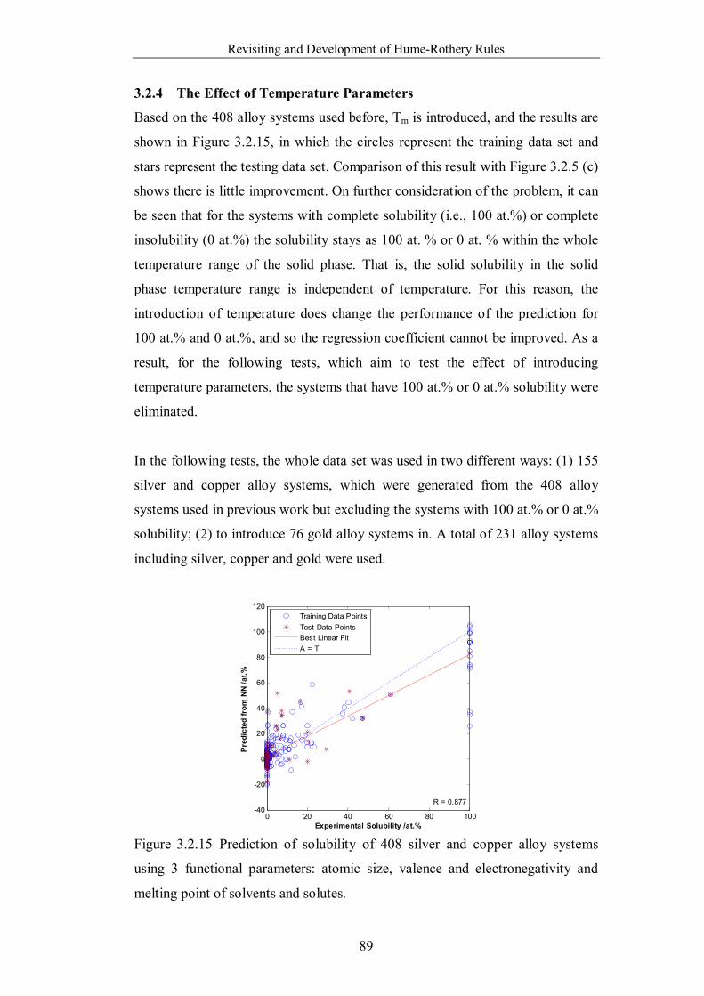
Revisiting and Development of Hume-Rothery Rules
89
3.2.4 The Effect of Temperature Parameters
Based on the 408 alloy systems used before, Tm is introduced, and the results are
shown in Figure 3.2.15, in which the circles represent the training data set and
stars represent the testing data set. Comparison of this result with Figure 3.2.5 (c)
shows there is little improvement. On further consideration of the problem, it can
be seen that for the systems with complete solubility (i.e., 100 at.%) or complete
insolubility (0 at.%) the solubility stays as 100 at. % or 0 at. % within the whole
temperature range of the solid phase. That is, the solid solubility in the solid
phase temperature range is independent of temperature. For this reason, the
introduction of temperature does change the performance of the prediction for
100 at.% and 0 at.%, and so the regression coefficient cannot be improved. As a
result, for the following tests, which aim to test the effect of introducing
temperature parameters, the systems that have 100 at.% or 0 at.% solubility were
eliminated.
In the following tests, the whole data set was used in two different ways: (1) 155
silver and copper alloy systems, which were generated from the 408 alloy
systems used in previous work but excluding the systems with 100 at.% or 0 at.%
solubility; (2) to introduce 76 gold alloy systems in. A total of 231 alloy systems
including silver, copper and gold were used.
0 20 40 60 80 100-40
-20
0
20
40
60
80
100
120
Experimental Solubility /at.%
Pred
icte
d fr
om N
N /a
t.%
R = 0.877
Training Data PointsTest Data PointsBest Linear FitA = T
Figure 3.2.15 Prediction of solubility of 408 silver and copper alloy systems
using 3 functional parameters: atomic size, valence and electronegativity and
melting point of solvents and solutes.
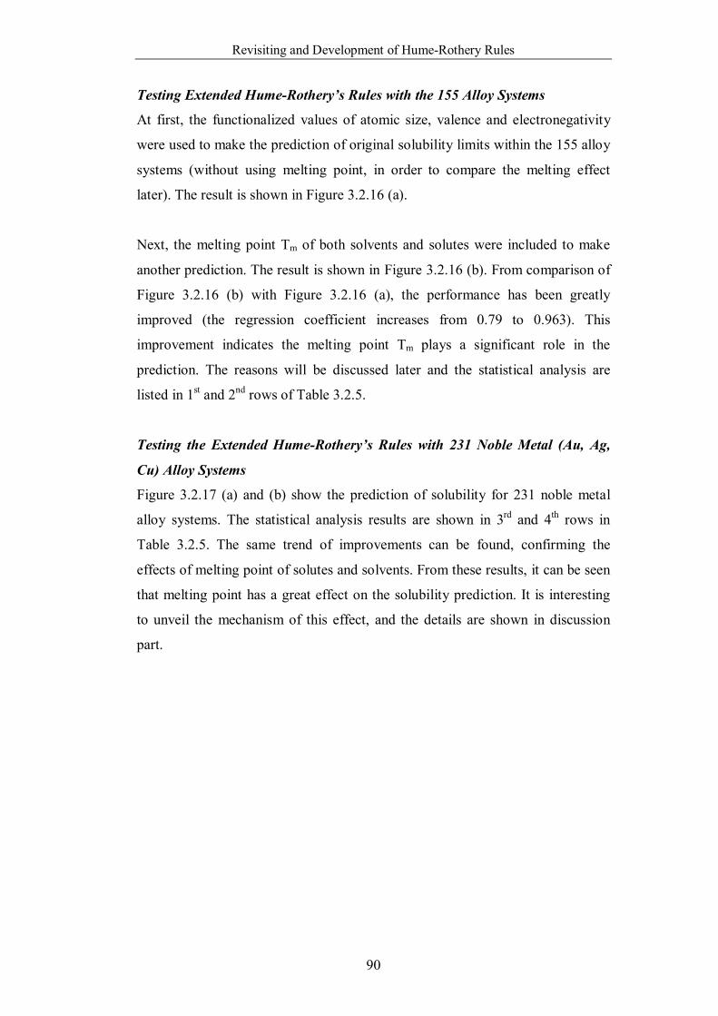
Revisiting and Development of Hume-Rothery Rules
90
Testing Extended Hume-Rothery’s Rules with the 155 Alloy Systems
At first, the functionalized values of atomic size, valence and electronegativity
were used to make the prediction of original solubility limits within the 155 alloy
systems (without using melting point, in order to compare the melting effect
later). The result is shown in Figure 3.2.16 (a).
Next, the melting point Tm of both solvents and solutes were included to make
another prediction. The result is shown in Figure 3.2.16 (b). From comparison of
Figure 3.2.16 (b) with Figure 3.2.16 (a), the performance has been greatly
improved (the regression coefficient increases from 0.79 to 0.963). This
improvement indicates the melting point Tm plays a significant role in the
prediction. The reasons will be discussed later and the statistical analysis are
listed in 1st and 2nd rows of Table 3.2.5.
Testing the Extended Hume-Rothery’s Rules with 231 Noble Metal (Au, Ag,
Cu) Alloy Systems
Figure 3.2.17 (a) and (b) show the prediction of solubility for 231 noble metal
alloy systems. The statistical analysis results are shown in 3rd and 4th rows in
Table 3.2.5. The same trend of improvements can be found, confirming the
effects of melting point of solutes and solvents. From these results, it can be seen
that melting point has a great effect on the solubility prediction. It is interesting
to unveil the mechanism of this effect, and the details are shown in discussion
part.
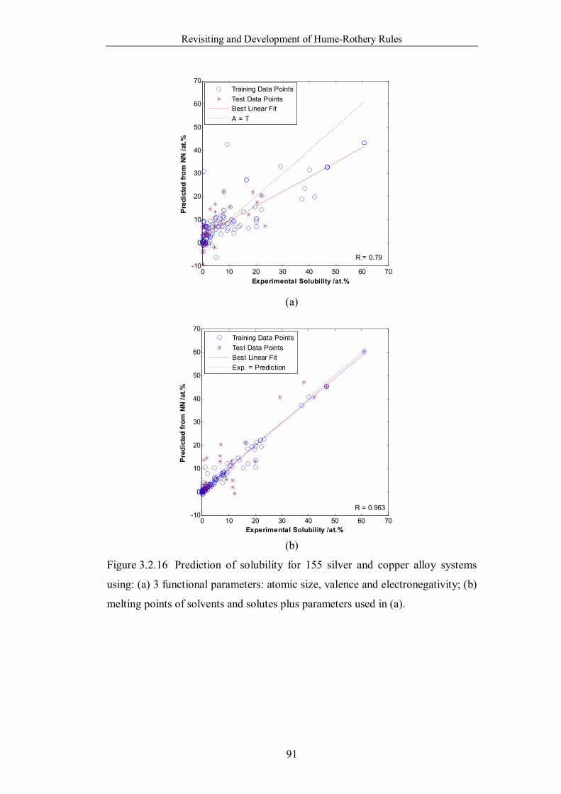
Revisiting and Development of Hume-Rothery Rules
91
0 10 20 30 40 50 60 70-10
0
10
20
30
40
50
60
70
Experimental Solubility /at.%
Pre
dict
ed fr
om N
N /a
t.%
R = 0.79
Training Data PointsTest Data PointsBest Linear FitA = T
(a)
0 10 20 30 40 50 60 70-10
0
10
20
30
40
50
60
70
Experimental Solubility /at.%
Pred
icte
d fr
om N
N /a
t.%
R = 0.963
Training Data PointsTest Data PointsBest Linear FitExp. = Prediction
(b)
Figure 3.2.16 Prediction of solubility for 155 silver and copper alloy systems
using: (a) 3 functional parameters: atomic size, valence and electronegativity; (b)
melting points of solvents and solutes plus parameters used in (a).
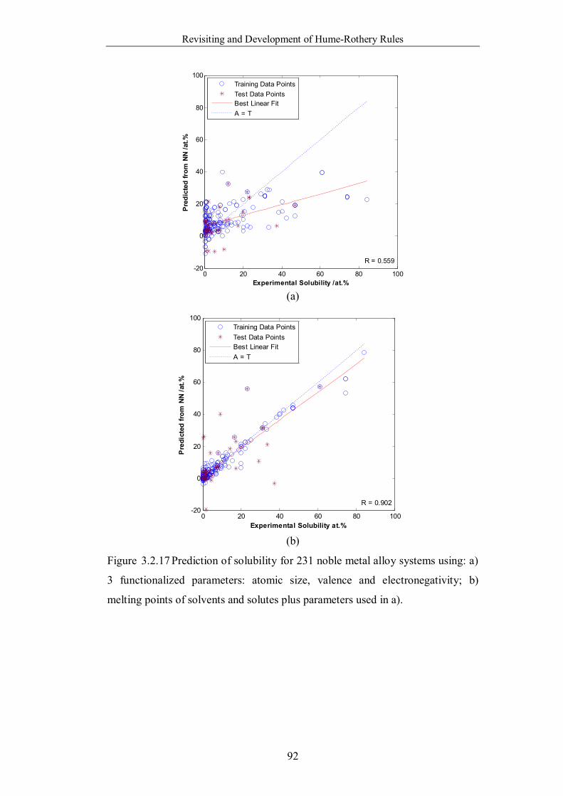
Revisiting and Development of Hume-Rothery Rules
92
0 20 40 60 80 100-20
0
20
40
60
80
100
Experimental Solubility /at.%
Pre
dict
ed fr
om N
N /a
t.%
R = 0.559
Training Data PointsTest Data PointsBest Linear FitA = T
(a)
0 20 40 60 80 100-20
0
20
40
60
80
100
Experimental Solubility at.%
Pre
dict
ed fr
om N
N /a
t.%
R = 0.902
Training Data PointsTest Data PointsBest Linear FitA = T
(b)
Figure 3.2.17 Prediction of solubility for 231 noble metal alloy systems using: a)
3 functionalized parameters: atomic size, valence and electronegativity; b)
melting points of solvents and solutes plus parameters used in a).
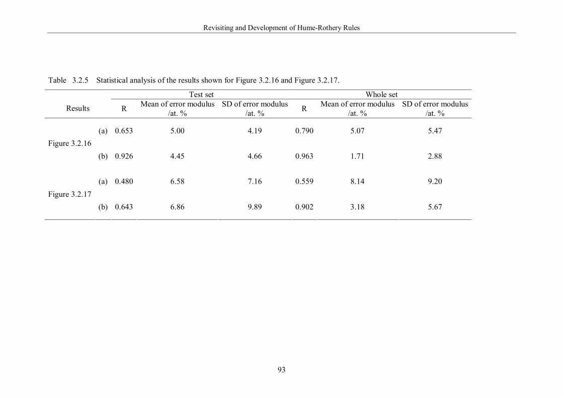
Revisiting and Development of Hume-Rothery Rules
93
Table 3.2.5 Statistical analysis of the results shown for Figure 3.2.16 and Figure 3.2.17.
Test set Whole set Results R Mean of error modulus
/at. % SD of error modulus
/at. % R Mean of error modulus /at. %
SD of error modulus /at. %
(a) 0.653 5.00 4.19 0.790 5.07 5.47 Figure 3.2.16
(b) 0.926 4.45 4.66 0.963 1.71 2.88
(a) 0.480 6.58 7.16 0.559 8.14 9.20 Figure 3.2.17
(b) 0.643 6.86 9.89 0.902 3.18 5.67
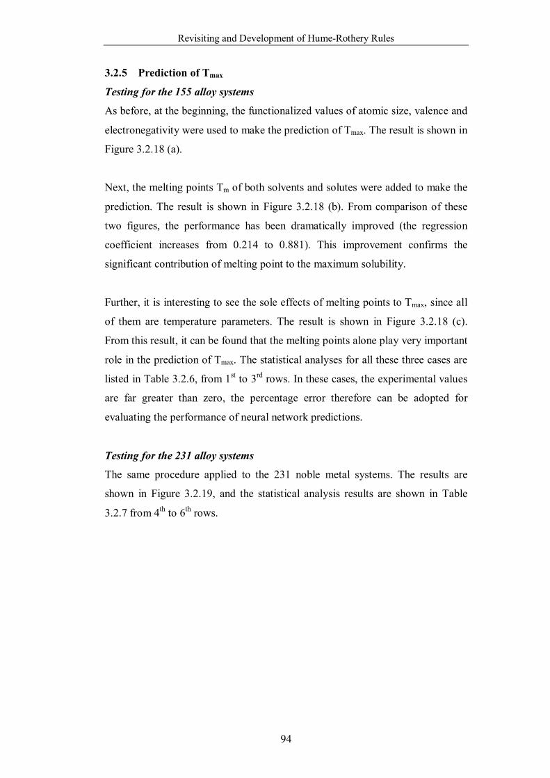
Revisiting and Development of Hume-Rothery Rules
94
3.2.5 Prediction of Tmax
Testing for the 155 alloy systems
As before, at the beginning, the functionalized values of atomic size, valence and
electronegativity were used to make the prediction of Tmax. The result is shown in
Figure 3.2.18 (a).
Next, the melting points Tm of both solvents and solutes were added to make the
prediction. The result is shown in Figure 3.2.18 (b). From comparison of these
two figures, the performance has been dramatically improved (the regression
coefficient increases from 0.214 to 0.881). This improvement confirms the
significant contribution of melting point to the maximum solubility.
Further, it is interesting to see the sole effects of melting points to Tmax, since all
of them are temperature parameters. The result is shown in Figure 3.2.18 (c).
From this result, it can be found that the melting points alone play very important
role in the prediction of Tmax. The statistical analyses for all these three cases are
listed in Table 3.2.6, from 1st to 3rd rows. In these cases, the experimental values
are far greater than zero, the percentage error therefore can be adopted for
evaluating the performance of neural network predictions.
Testing for the 231 alloy systems
The same procedure applied to the 231 noble metal systems. The results are
shown in Figure 3.2.19, and the statistical analysis results are shown in Table
3.2.7 from 4th to 6th rows.
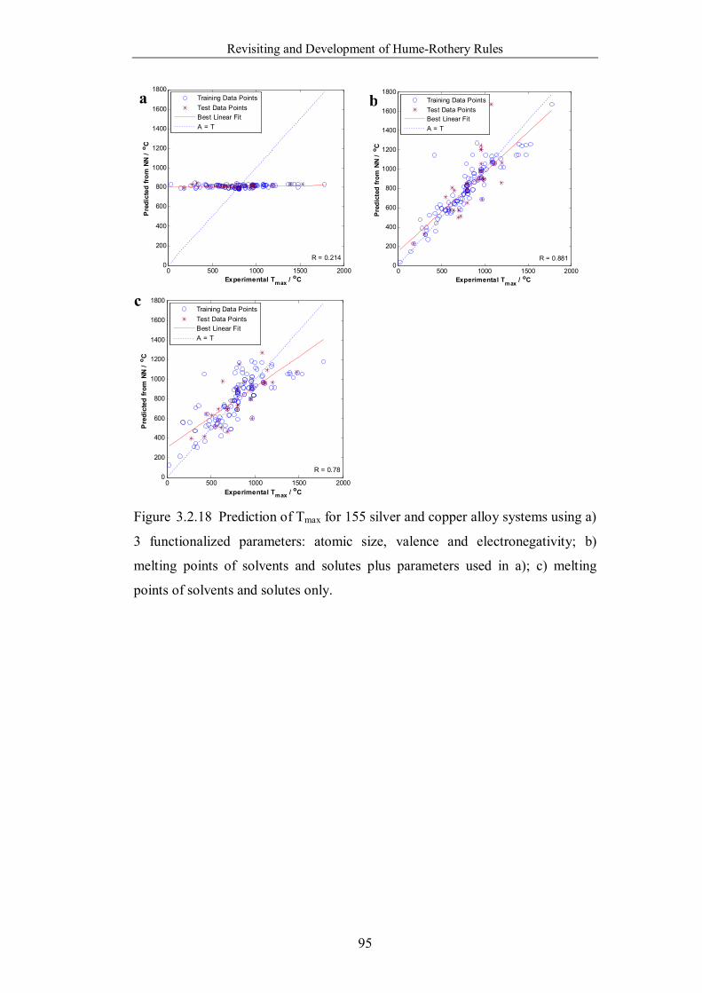
Revisiting and Development of Hume-Rothery Rules
95
0 500 1000 1500 20000
200
400
600
800
1000
1200
1400
1600
1800
Experimental Tmax / oC
Pre
dict
ed fr
om N
N /
o C
R = 0.214
Training Data PointsTest Data PointsBest Linear FitA = T
0 500 1000 1500 2000
0
200
400
600
800
1000
1200
1400
1600
1800
Experimental Tmax / oC
Pred
icte
d fro
m N
N /
o C
R = 0.881
Training Data PointsTest Data PointsBest Linear FitA = T
0 500 1000 1500 20000
200
400
600
800
1000
1200
1400
1600
1800
Experimental Tmax / oC
Pre
dict
ed fr
om N
N /
o C
R = 0.78
Training Data PointsTest Data PointsBest Linear FitA = T
Figure 3.2.18 Prediction of Tmax for 155 silver and copper alloy systems using a)
3 functionalized parameters: atomic size, valence and electronegativity; b)
melting points of solvents and solutes plus parameters used in a); c) melting
points of solvents and solutes only.
b
c
a
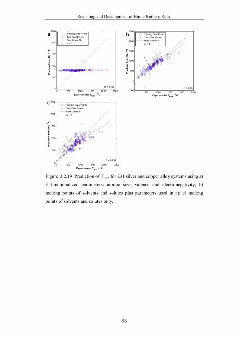
Revisiting and Development of Hume-Rothery Rules
96
0 500 1000 1500 2000 25000
500
1000
1500
2000
2500
Experimental Tmax / oC
Pred
icte
d fro
m N
N /
o C
R = 0.168
Training Data PointsTest Data PointsBest Linear FitA = T
0 500 1000 1500 2000 2500
-500
0
500
1000
1500
2000
2500
Experimental Tmax / oC
Pred
icte
d fro
m N
N /
o C
R = 0.86
Training Data PointsTest Data PointsBest Linear FitA = T
0 500 1000 1500 2000 25000
500
1000
1500
2000
2500
Experimental Tmax / oC
Pred
icte
d fr
om N
N /
o C
R = 0.793
Training Data PointsTest Data PointsBest Linear FitA = T
Figure 3.2.19 Prediction of Tmax for 231 silver and copper alloy systems using a)
3 functionalized parameters: atomic size, valence and electronegativity; b)
melting points of solvents and solutes plus parameters used in a); c) melting
points of solvents and solutes only.
ba
c
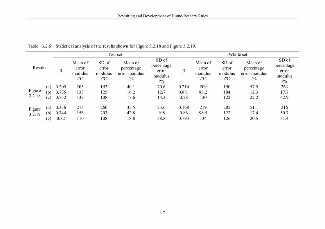
Revisiting and Development of Hume-Rothery Rules
97
Table 3.2.6 Statistical analysis of the results shown for Figure 3.2.18 and Figure 3.2.19.
Test set Whole set
Results R
Mean of error
modulus /ºC
SD of error
modulus /ºC
Mean of percentage
error modulus /%
SD of percentage
error modulus
/%
R
Mean of error
modulus /ºC
SD of error
modulus /ºC
Mean of percentage
error modulus /%
SD of percentage
error modulus
/% (a) 0.205 205 193 40.1 70.6 0.214 209 190 57.5 263 (b) 0.775 133 125 16.2 12.7 0.881 88.2 104 12.3 17.7 Figure
3.2.18 (c) 0.752 137 108 17.6 14.3 0.78 130 122 22.2 42.9
(a) 0.336 213 260 35.5 73.6 0.168 219 205 51.1 216 (b) 0.744 156 203 42.8 108 0.86 98.5 123 17.4 50.7
Figure 3.2.19
(c) 0.82 110 108 18.8 38.8 0.793 134 126 20.5 31.4
Revisiting and Development of Hume-Rothery Rules
98
3.3 Discussion
It is important to recognize that there are four different factors that limit the
predictive capability of the networks: (i) imperfections in the network
configuration which we have attempted to minimize through design, (ii) paucity
of learning data which has been mentioned in section 2.0, (iii) the generality of
Hume-Rothery’s Rules which were conceived as guidelines and (iv) the fact,
recognized by Hume-Rothery and co-authors, that the available data are subject
to inexactitudes.
3.3.1 The Reliability of Input Parameters
Hume-Rothery et al. (1934) themselves made it clear that the exact “atomic
diameter” of an element is always difficult to define. Their definition of atomic
diameter, as given by the nearest-neighbour distance in a crystal of the pure
metal, was used here but the “radius” of an atom is probably affected by
coordination number. Except for the heavy elements, elements of the B sub-
groups tend to crystallize with coordination number 8-N, where N is the group to
which the element belongs. This is due to the partly covalent nature of the forces
in these crystals, and except in Group IV B (diamond structure) results in the
atoms having two sets of neighbours at different distances in the crystal. Cottrell
(1998) suggests that the concept of a characteristic size, which suggests hard
spheres butted together, is doubtful. Allocating a single atomic diameter for each
element, independent of its environment, and valences of solvent and solute is
too simplistic an approach (Hume-Rothery et al., 1969). Furthermore, within the
408 alloy systems, the metallic radius of some elements could not be found and
covalent radius used instead. These factors contribute to the errors for the
prediction of solid solubility limit and are to be distinguished from intrinsic
weakness of the ANN.
An early discovery by Hume-Rothery was that a metal of lower valence is more
likely to dissolve one of higher valence than vice versa. However, more detailed
examination has not confirmed this. As mentioned before, silver dissolves about
20% aluminium but aluminium dissolves about 24% silver. For high valence,
covalently bonded components, the relative valence factor applies. For example,
copper dissolves about 11% of silicon, which behaves as a 4-valent metal in
Revisiting and Development of Hume-Rothery Rules
99
forming Cu-Si electron phase alloys, but the solubility of copper in covalently
bonded silicon is negligible (Cottrell, 1998). As a result, although Hume-
Rothery (Hume-Rothery et al., 1969) accepted that it is still a general principle
that the solubility in the element of lower valency is of greater extent when
dealing with alloys of univalent metals copper, silver and gold with metals with
higher valency, in its general form, this principle must be treated with caution.
Also, the valencies of transition metals are variable and complex and have been
analyzed by Hume-Rothery et al. (1951) and Cockayne and Raynor (1961). As
suggested by Cottrell (1998), due to the valency complication caused by partly-
filled d shells, the transition metal alloys generally do not follow the rule.
Gschneider (1980) modified the relative valence rule so that the solubility is low
when a metal in which d orbitals strongly influence the valence behaviour, is
alloyed with a simple ‘sp metal’, but that the solubility is likely to be better in the
d metal than the reverse.
The electronegativity rule needs a scale, such as that given by Mulliken, based on
the equation AI21
, where I is the ionization energy, A is electron affinity
and χ is Mulliken electronegativity. When divided by 2.8, this scale matches the
empirical scale of Pauling reasonably well. In the case of transition metals, as
emphasized by Watson and Bennett (1978), the partly-filled d states of transition
metals at energies near the Fermi energy influence electronegativity. Watson and
Bennett presented an electronegativity scale for transition metals that matched
Pauling’s scale, and could be scaled by 2.8 to bring it to Mulliken’s scale of χ
values. Most importantly, Li and Xue (2006) recently have mentioned that
“although electronegativity is often treated as an invariant property of an atom,
as in Pauling’s scale, it actually depends on the chemical environment of the
atom, e.g. valence state and coordination number”, which was also mentioned in
Hume-Rothery et al. (1969). The electronegativity values adopted in this part of
work are based on Pauling’s work, so the above effects are not entirely taken into
account.
Revisiting and Development of Hume-Rothery Rules
100
The method adopted for expressing structure parameter has some limitations.
Firstly, the expressions used to distinguish different crystal structures can
conceal similarities. For unit cell length, a=b=c and a=b≠c are distinguished but
can have considerable similarity. Secondly, from this expression, the face
centered cubic (FCC) and the hexagonal close packed (HCP) systems are
expressed as quite distinct sets but there are some similarities between these two
structures. They are both close packed systems and stacking faults can blur the
difference. Indeed the Cu and Zn systems demonstrate high solubility even
though one component, Zn, is HCP and the Cu is FCC. The Ag and α-Li system
is a similar case. Thirdly, there are several complex structural systems that
cannot be distinguished from other systems by using this expression, such as α-
Mn, whose structure is cI58, and β-Mn, whose structure is cP20. These all affect
the ability of the structure parameter to contribute to predicting the solubility.
3.3.2 The Effect of Melting Point
The melting point effect actually has been interpreted from some aspects by
Hume-Rothery et al. (Buckley and Hume-Rothery, 1963; Hume-Rothery,
1965). The solid solubility of an alloy system can be treated as the capability to
stabilize in the solid phase at that solubility value of added elements, under a
certain temperature and this is the competition between the liquid and solid phase
for these conditions (certain solubility values and temperature) under free energy
minimisation routine. Hume-Rothery et al. assessed the stabilizing power of
liquid and solid phase in terms of the free energy difference (ΔG), which is the
free energy of transfer one mole of solute from the solid to the liquid phase, and
includes the melting point effect and other effects (such as atomic diameters,
electronic effects, etc.). This can be written as
FmpfG Equation 3.3.1
where the mpf is the melting point effect, and F is the effect due to atomic
diameters, electronic effects and so on.
From Equation 3.3.1, it can be seen that the stability of one phase can be
interpreted in terms of size effects, electronic effects, melting points etc. The
effects that contribute to F actually are the parameters in Hume-Rothery’s

Revisiting and Development of Hume-Rothery Rules
101
Rules, as mentioned in a previous paper (Zhang et al., 2008); and the melting
point effect is the extra effect. For detail, the melting point effect mpf can be
expressed as TSF , where FS is the entropy of freezing of solute element,
and T is the difference between T and the melting point of the pure solute.
The above equation explains the effect of melting points of solutes and the
temperature at which the stable phase is obtained. This is why the performance of
solubility prediction can be improved by introducing the melting point of solutes
and the temperature at which the maximum solubility is attained.
3.3.3 The Generality of Hume-Rothery’s Rules
Hume-Rothery and co-workers state: “In general, the solubility limit is mainly
determined by these factors, and it is their interplay that makes the results so
complex” (Hume-Rothery et al., 1934). For the 60 alloy systems mentioned by
Hume-Rothery in 1934, and using some of the parameter values that can be
found in Hume-Rothery’s paper or his book and others that follow his
representations, the results for prediction of solid solubility limit are satisfactory.
However, from theory as analyzed by others in later work (Zhang and Liao,
1999a, b; Cottrell, 1998; Miedema, 1973), and also from the attempts to predict
solid solubility limit of the 408 alloy systems, it can be said that Hume-Rothery’s
Rules work properly in a certain range of alloy systems, but cannot be treated as
general principles. Also it needs to be said that despite using Hume-Rothery’s
Rules, one cannot predict the solid solubility limits accurately. However, these
rules are still useful guidelines for judging the solubility of alloy systems.
Further, the introduction of the melting temperatures of both solvents and solutes
has a significant effect for the prediction of solid solubility values and its related
parameter Tmax.
The Policing and Correction of Handbooks and Databases by ANNs
102
4.0 The Policing and Correction of Handbooks and Databases
by Artificial Neural Networks 4.1 Data Collection
In this work, the properties of the elements were used as a test dataset for
scrutiny by the ANN since these data were expected to be very reliable. Only
elements with short half lives were excluded. The majority were taken from
Chemistry Data Handbook (CDH) (Stark and Wallace, 1982). When suspects
were identified, more handbooks were called upon including The Lange’s
Handbook of Chemistry (LHC) (Speight, 2005), The Elements (ELE) (Emsley,
1998), Tables of Physical and Chemical Constants (TPC) (Kaye and Laby, 1995)
and CRC Handbook of Chemistry and Physics (CRC) (David, 2000).
4.2 General Steps for Policing/Correction of Errors and Results
This process involves four different stages.
Stage 1: A dataset is examined for internal relationships and inconsistent data-
points are identified. In one example, the ANN was used to explore the indirect
relationship between boiling point and enthalpy of vaporization using data from
CDH (Table 4.1.1 and Figure 4.1.1). The best linear fit equations have regression
coefficients R=0.973 and 0.972. On this basis, the correlation hypothesis was
raised that the correlation applies to all elements. However, some data points fall
well away from the line: e.g. Ho, Se, S, Te, I, As (α), Nb, P, Cd and Pd for which
there are two possible causes. The first is that the correlation hypothesis is
violated for these special cases; and the second is incorrect handbook data. So at
this stage, data from other sources (ELE, TPC and CRC), if available, are
brought in (Table 4.1.2 and 4.1.3).
Table 4.1.1 The dataset used to train the ANN shown in Figure 4.1.1. Majority
were taken from Chemistry Data Handbook (CDH, 1982) without judgement. A
few data unavailable in CDH were taken from LAG and ELE. (BP: Boiling Point;
ΔHV: Enthalpy of Vaporization).
Elements BP /K ΔHv /kJ mol-1 Elements BP /K ΔHv
/kJ mol-1 Elements BP /K ΔHv /kJ mol-1
Ag 2483 254 H 21.15 0.90 Pt 4803 510 Al 2743 284 He 4.150 0.08 Rb 961.2 69.0 Ar 87.20 6.53 Hf 5673 648 Re 5903 636
As (grey) 886.2 32.4 Ho 2873 71.0 Rh 4773 531
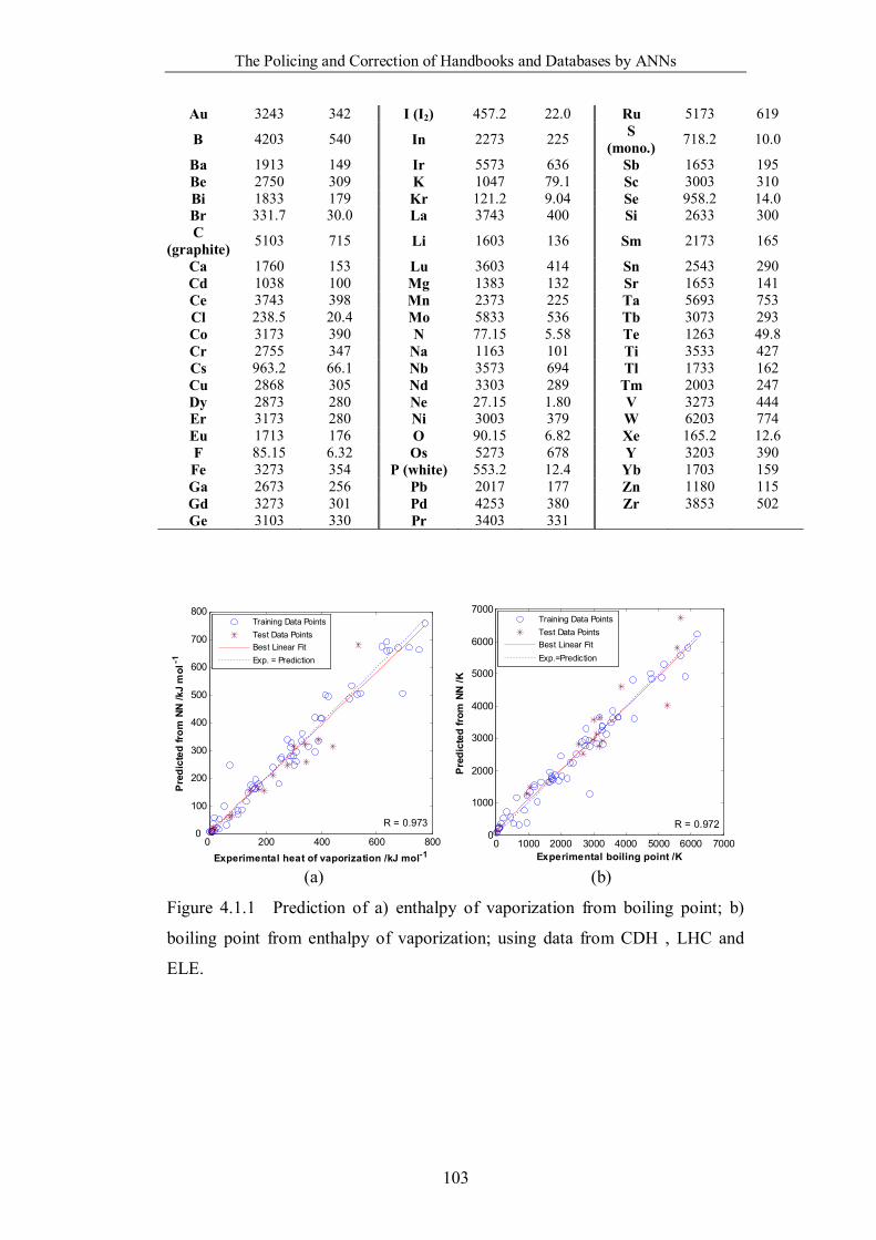
The Policing and Correction of Handbooks and Databases by ANNs
103
Au 3243 342 I (I2) 457.2 22.0 Ru 5173 619
B 4203 540 In 2273 225 S (mono.) 718.2 10.0
Ba 1913 149 Ir 5573 636 Sb 1653 195 Be 2750 309 K 1047 79.1 Sc 3003 310 Bi 1833 179 Kr 121.2 9.04 Se 958.2 14.0 Br 331.7 30.0 La 3743 400 Si 2633 300 C
(graphite) 5103 715 Li 1603 136 Sm 2173 165
Ca 1760 153 Lu 3603 414 Sn 2543 290 Cd 1038 100 Mg 1383 132 Sr 1653 141 Ce 3743 398 Mn 2373 225 Ta 5693 753 Cl 238.5 20.4 Mo 5833 536 Tb 3073 293 Co 3173 390 N 77.15 5.58 Te 1263 49.8 Cr 2755 347 Na 1163 101 Ti 3533 427 Cs 963.2 66.1 Nb 3573 694 Tl 1733 162 Cu 2868 305 Nd 3303 289 Tm 2003 247 Dy 2873 280 Ne 27.15 1.80 V 3273 444 Er 3173 280 Ni 3003 379 W 6203 774 Eu 1713 176 O 90.15 6.82 Xe 165.2 12.6 F 85.15 6.32 Os 5273 678 Y 3203 390 Fe 3273 354 P (white) 553.2 12.4 Yb 1703 159 Ga 2673 256 Pb 2017 177 Zn 1180 115 Gd 3273 301 Pd 4253 380 Zr 3853 502 Ge 3103 330 Pr 3403 331
0 200 400 600 8000
100
200
300
400
500
600
700
800
Experimental heat of vaporization /kJ mol-1
Pre
dict
ed fr
om N
N /k
J m
ol-1
R = 0.973
Training Data PointsTest Data PointsBest Linear FitExp. = Prediction
0 1000 2000 3000 4000 5000 6000 70000
1000
2000
3000
4000
5000
6000
7000
Experimental boiling point /K
Pre
dict
ed fr
om N
N /K
R = 0.972
Training Data PointsTest Data PointsBest Linear FitExp.=Prediction
(a) (b)
Figure 4.1.1 Prediction of a) enthalpy of vaporization from boiling point; b)
boiling point from enthalpy of vaporization; using data from CDH , LHC and
ELE.
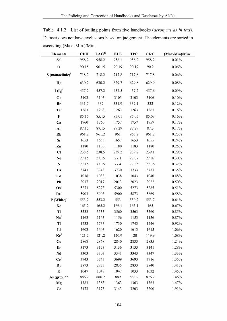
The Policing and Correction of Handbooks and Databases by ANNs
104
Table 4.1.2 List of boiling points from five handbooks (acronyms as in text).
Dataset does not have exclusions based on judgement. The elements are sorted in
ascending (Max.-Min.)/Min.
Elements CDH LAG& ELE TPC CRC (Max-Min)/Min SeI 958.2 958.2 958.1 958.2 958.2 0.01%
O 90.15 90.15 90.19 90.19 90.2 0.06%
S (monoclinic)I 718.2 718.2 717.8 717.8 717.8 0.06%
Hg 630.2 630.2 629.7 629.8 629.9 0.08%
I (I2)I 457.2 457.2 457.5 457.2 457.6 0.09%
Ge 3103 3103 3103 3103 3106 0.10% Br 331.7 332 331.9 332.1 332 0.12%
TeI 1263 1263 1263 1263 1261 0.16%
F 85.15 85.15 85.01 85.05 85.03 0.16% Ca 1760 1760 1757 1757 1757 0.17% Ar 87.15 87.15 87.29 87.29 87.3 0.17% Rb 961.2 961.2 961 963.2 961.2 0.23% Sr 1653 1653 1657 1653 1655 0.24% Zn 1180 1180 1180 1183 1180 0.25% Cl 238.5 238.5 239.2 239.2 239.1 0.29% Ne 27.15 27.15 27.1 27.07 27.07 0.30% N 77.15 77.15 77.4 77.35 77.36 0.32% La 3743 3743 3730 3733 3737 0.35% Cd 1038 1038 1038 1043 1040 0.48% Pb 2017 2017 2013 2023 2022 0.50% OsI 5273 5273 5300 5273 5285 0.51% ReI 5903 5903 5900 5873 5869 0.58%
P (White)I 553.2 553.2 553 550.2 553.7 0.64% Xe 165.2 165.2 166.1 165.1 165 0.67% Ti 3533 3533 3560 3563 3560 0.85%
NaI 1163 1163 1156 1153 1156 0.87% Tl 1733 1733 1730 1743 1746 0.92% Li 1603 1603 1620 1613 1615 1.06%
KrI 121.2 121.2 120.9 120 119.9 1.08% Cu 2868 2868 2840 2833 2835 1.24% Er 3173 3173 3136 3133 3141 1.28% Nd 3303 3303 3341 3343 3347 1.33% CeI 3743 3743 3699 3693 3716 1.35% Dy 2873 2873 2835 2833 2840 1.41% K 1047 1047 1047 1033 1032 1.45%
As (grey)** 886.2 886.2 889 883.2 876.2 1.46% Mg 1383 1383 1363 1363 1363 1.47% Co 3173 3173 3143 3203 3200 1.91%
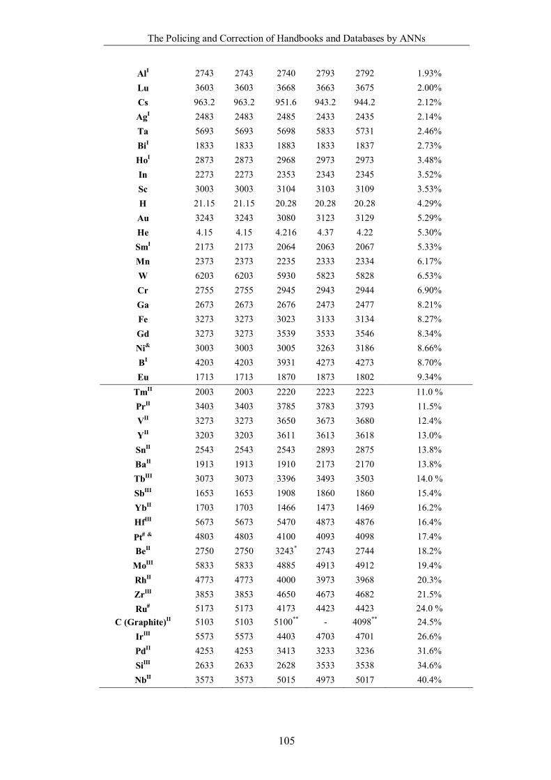
The Policing and Correction of Handbooks and Databases by ANNs
105
AlI 2743 2743 2740 2793 2792 1.93% Lu 3603 3603 3668 3663 3675 2.00% Cs 963.2 963.2 951.6 943.2 944.2 2.12% AgI 2483 2483 2485 2433 2435 2.14% Ta 5693 5693 5698 5833 5731 2.46% BiI 1833 1833 1883 1833 1837 2.73% HoI 2873 2873 2968 2973 2973 3.48% In 2273 2273 2353 2343 2345 3.52% Sc 3003 3003 3104 3103 3109 3.53% H 21.15 21.15 20.28 20.28 20.28 4.29% Au 3243 3243 3080 3123 3129 5.29% He 4.15 4.15 4.216 4.37 4.22 5.30% SmI 2173 2173 2064 2063 2067 5.33% Mn 2373 2373 2235 2333 2334 6.17% W 6203 6203 5930 5823 5828 6.53% Cr 2755 2755 2945 2943 2944 6.90% Ga 2673 2673 2676 2473 2477 8.21% Fe 3273 3273 3023 3133 3134 8.27% Gd 3273 3273 3539 3533 3546 8.34% Ni& 3003 3003 3005 3263 3186 8.66% BI 4203 4203 3931 4273 4273 8.70% Eu 1713 1713 1870 1873 1802 9.34%
TmII 2003 2003 2220 2223 2223 11.0 % PrII 3403 3403 3785 3783 3793 11.5% VII 3273 3273 3650 3673 3680 12.4% YII 3203 3203 3611 3613 3618 13.0% SnII 2543 2543 2543 2893 2875 13.8% BaII 1913 1913 1910 2173 2170 13.8% TbIII 3073 3073 3396 3493 3503 14.0 % SbIII 1653 1653 1908 1860 1860 15.4% YbII 1703 1703 1466 1473 1469 16.2% HfIII 5673 5673 5470 4873 4876 16.4%
Pt & 4803 4803 4100 4093 4098 17.4% BeII 2750 2750 3243* 2743 2744 18.2%
MoIII 5833 5833 4885 4913 4912 19.4% RhII 4773 4773 4000 3973 3968 20.3% ZrIII 3853 3853 4650 4673 4682 21.5% Ru 5173 5173 4173 4423 4423 24.0 %
C (Graphite)II 5103 5103 5100** - 4098** 24.5% IrIII 5573 5573 4403 4703 4701 26.6% PdII 4253 4253 3413 3233 3236 31.6% SiIII 2633 2633 2628 3533 3538 34.6% NbII 3573 3573 5015 4973 5017 40.4%

The Policing and Correction of Handbooks and Databases by ANNs
106
* Under pressure
** Sublimation
& the boiling point is different in different tables of LAG. For example, Nickel (Ni) is
2884C in Page 1.43 (Table 1.3) and 2730C in page 1.125 (Table 1.19). We selected
most of the boiling points from the later table.
The variation of boiling points of Pt and Ru are greater than 10% but here due to
shortage of data in range of 3603.15 to 5693.15 K in Category IV, they were classified
into Category IV by identifying the closest value from the literature to reduce the
uncertainty in that range (Arblaster, 2005; 2007).
I. Category I: The data of boiling point for these elements are consistent in different
handbooks but that of enthalpy of vaporization are not.
II. Category II: The data of enthalpy of vaporization for these elements are consistent in
different handbooks but that of boiling point are not.
III. Category III: The data of neither boiling point nor enthalpy of vaporization for these
elements are consistent in different handbooks
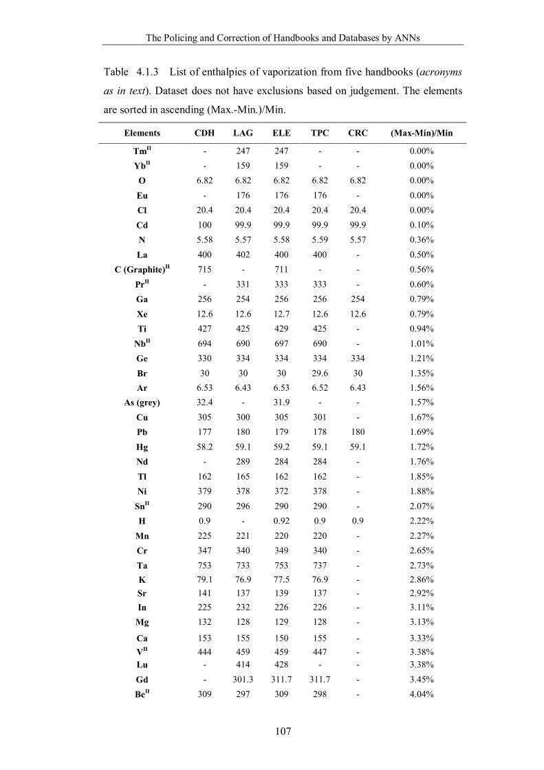
The Policing and Correction of Handbooks and Databases by ANNs
107
Table 4.1.3 List of enthalpies of vaporization from five handbooks (acronyms
as in text). Dataset does not have exclusions based on judgement. The elements
are sorted in ascending (Max.-Min.)/Min.
Elements CDH LAG ELE TPC CRC (Max-Min)/Min
TmII - 247 247 - - 0.00% YbII - 159 159 - - 0.00%
O 6.82 6.82 6.82 6.82 6.82 0.00%
Eu - 176 176 176 - 0.00% Cl 20.4 20.4 20.4 20.4 20.4 0.00%
Cd 100 99.9 99.9 99.9 99.9 0.10% N 5.58 5.57 5.58 5.59 5.57 0.36%
La 400 402 400 400 - 0.50% C (Graphite)II 715 - 711 - - 0.56%
PrII - 331 333 333 - 0.60% Ga 256 254 256 256 254 0.79%
Xe 12.6 12.6 12.7 12.6 12.6 0.79% Ti 427 425 429 425 - 0.94%
NbII 694 690 697 690 - 1.01% Ge 330 334 334 334 334 1.21%
Br 30 30 30 29.6 30 1.35% Ar 6.53 6.43 6.53 6.52 6.43 1.56%
As (grey) 32.4 - 31.9 - - 1.57%
Cu 305 300 305 301 - 1.67% Pb 177 180 179 178 180 1.69%
Hg 58.2 59.1 59.2 59.1 59.1 1.72% Nd - 289 284 284 - 1.76%
Tl 162 165 162 162 - 1.85% Ni 379 378 372 378 - 1.88%
SnII 290 296 290 290 - 2.07% H 0.9 - 0.92 0.9 0.9 2.22%
Mn 225 221 220 220 - 2.27% Cr 347 340 349 340 - 2.65%
Ta 753 733 753 737 - 2.73% K 79.1 76.9 77.5 76.9 - 2.86% Sr 141 137 139 137 - 2.92% In 225 232 226 226 - 3.11%
Mg 132 128 129 128 - 3.13%
Ca 153 155 150 155 - 3.33% VII 444 459 459 447 - 3.38% Lu - 414 428 - - 3.38%
Gd - 301.3 311.7 311.7 - 3.45% BeII 309 297 309 298 - 4.04%
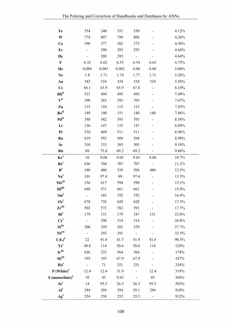
The Policing and Correction of Handbooks and Databases by ANNs
108
Fe 354 340 351 350 - 4.12% W 774 807 799 806 - 4.26%
Co 390 377 382 373 - 4.56% Er - 280 293 293 - 4.64%
Dy - 280 293 - - 4.64% F 6.32 6.62 6.55 6.54 6.62 4.75%
He 0.084 0.083 0.082 0.08 0.08 5.00% Ne 1.8 1.71 1.74 1.77 1.71 5.26%
Au 342 324 324 324 324 5.56% Cs 66.1 63.9 65.9 67.8 - 6.10%
RhII 531 494 495 495 - 7.49% YII 390 365 393 393 - 7.67%
Zn 115 124 115 115 - 7.83% BaII 149 140 151 140 140 7.86%
PdII 380 362 393 393 - 8.56% Li 136 147 135 147 - 8.89%
Pt 510 469 511 511 - 8.96% Ru 619 592 568 568 - 8.98%
Sc 310 333 305 305 - 9.18% Rb 69 75.8 69.2 69.2 - 9.86%
KrI 10 9.08 9.05 9.03 9.08 10.7% ReI 636 704 707 707 - 11.2% BI 540 480 539 508 480 12.5%
NaI 101 97.4 89 97.4 - 13.5% MoIII 536 617 594 590 - 15.1%
HfIII 648 571 661 661 - 15.8% SmI - 165 192 192 - 16.4%
OsI 678 738 628 628 - 17.5% ZrIII 502 573 582 591 - 17.7%
BiI 179 151 179 187 151 23.8% CeI - 398 314 314 - 26.8%
SiIII 300 359 383 359 - 27.7% TbIII - 293 391 - - 33.5%
I (I2)I 22 41.6 41.7 41.9 41.6 90.5% TeI 49.8 114 50.6 50.6 114 129%
IrIII 636 232 564 564 - 174% SbIII 195 193 67.9 67.9 - 187%
HoI - 71 251 251 - 254% P (White)I 12.4 12.4 51.9 - 12.4 319%
S (monoclinic)I 10 45 9.62 - 45 368% SeI 14 95.5 26.3 26.3 95.5 582%
AlI 284 294 294 29.1 294 910% AgI 254 258 255 25.5 - 912%

The Policing and Correction of Handbooks and Databases by ANNs
109
I. Category I: The data for boiling point for these elements are consistent in different
handbooks but those for enthalpy of vaporization are not.
II. Category II: The data for enthalpy of vaporization for these elements are consistent in
different handbooks but those of boiling point are not.
III. Category III: The data for neither boiling point nor enthalpy of vaporization for these
elements are consistent in different handbooks
Stage 2: This involves the selection of a conformity criterion. Remarkably, there
were 21 elements having inconsistent boiling point at the 10% level or above;
and 23 elements having inconsistent enthalpy of vaporization at the 10% level or
above in these five handbooks. These are not trivial numbers in only 82 elements
inspected and this is far above Chapman’s 1-5% field error rate (Chapman,
2005). Elements were then classified into four categories on the basis of a 10%
variation between minimum and maximum values (a full list of categories is in
Table 4.1.4 – 4.1.7):
I) boiling points of the elements are consistent but enthalpy of vaporization
are inconsistent;
II) enthalpy of vaporization are consistent but boiling points are inconsistent;
III) both boiling point and enthalpy of vaporization are inconsistent and;
IV) both boiling point and enthalpy of vaporization are consistent.
Consistency across the five handbooks does not imply accuracy (all could have
been copied from the same incorrect source) but the ANN may still detect a
deviation from the correlation line.
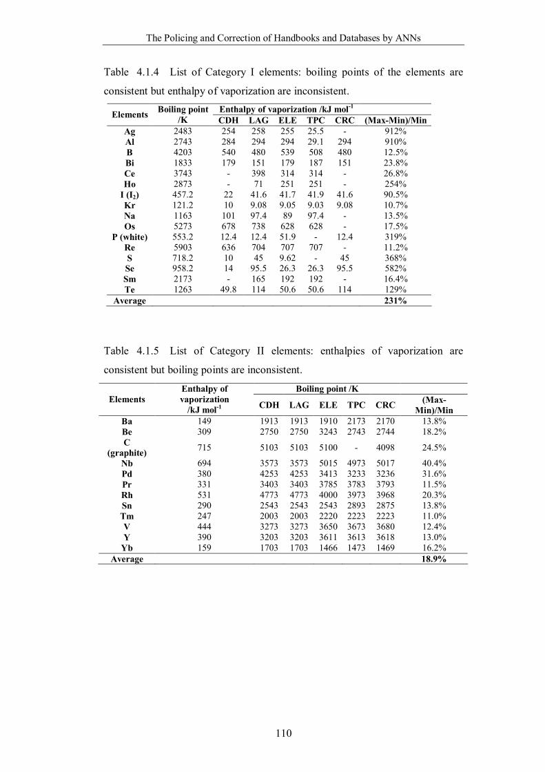
The Policing and Correction of Handbooks and Databases by ANNs
110
Table 4.1.4 List of Category I elements: boiling points of the elements are
consistent but enthalpy of vaporization are inconsistent. Enthalpy of vaporization /kJ mol-1 Elements Boiling point
/K CDH LAG ELE TPC CRC (Max-Min)/Min Ag 2483 254 258 255 25.5 - 912% Al 2743 284 294 294 29.1 294 910% B 4203 540 480 539 508 480 12.5% Bi 1833 179 151 179 187 151 23.8% Ce 3743 - 398 314 314 - 26.8% Ho 2873 - 71 251 251 - 254%
I (I2) 457.2 22 41.6 41.7 41.9 41.6 90.5% Kr 121.2 10 9.08 9.05 9.03 9.08 10.7% Na 1163 101 97.4 89 97.4 - 13.5% Os 5273 678 738 628 628 - 17.5%
P (white) 553.2 12.4 12.4 51.9 - 12.4 319% Re 5903 636 704 707 707 - 11.2% S 718.2 10 45 9.62 - 45 368% Se 958.2 14 95.5 26.3 26.3 95.5 582% Sm 2173 - 165 192 192 - 16.4% Te 1263 49.8 114 50.6 50.6 114 129%
Average 231%
Table 4.1.5 List of Category II elements: enthalpies of vaporization are
consistent but boiling points are inconsistent.
Boiling point /K Elements
Enthalpy of vaporization
/kJ mol-1 CDH LAG ELE TPC CRC (Max-Min)/Min
Ba 149 1913 1913 1910 2173 2170 13.8% Be 309 2750 2750 3243 2743 2744 18.2% C
(graphite) 715 5103 5103 5100 - 4098 24.5%
Nb 694 3573 3573 5015 4973 5017 40.4% Pd 380 4253 4253 3413 3233 3236 31.6% Pr 331 3403 3403 3785 3783 3793 11.5% Rh 531 4773 4773 4000 3973 3968 20.3% Sn 290 2543 2543 2543 2893 2875 13.8% Tm 247 2003 2003 2220 2223 2223 11.0% V 444 3273 3273 3650 3673 3680 12.4% Y 390 3203 3203 3611 3613 3618 13.0%
Yb 159 1703 1703 1466 1473 1469 16.2% Average 18.9%
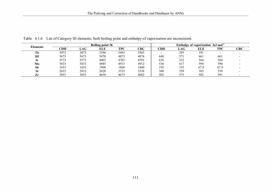
The Policing and Correction of Handbooks and Databases by ANNs
111
Table 4.1.6 List of Category III elements: both boiling point and enthalpy of vaporization are inconsistent. Boiling point /K Enthalpy of vaporization /kJ mol-1 Elements CDH LAG ELE TPC CRC CDH LAG ELE TPC CRC
Tb 3073 3073 3396 3493 3503 - 293 391 - - Hf 5673 5673 5470 4873 4876 648 571 661 661 - Ir 5573 5573 4403 4703 4701 636 232 564 564 -
Mo 5833 5833 4885 4913 4912 536 617 594 590 - Sb 1653 1653 1908 1860 1860 195 193 67.9 67.9 - Si 2633 2633 2628 3533 3538 300 359 383 359 - Zr 3853 3853 4650 4673 4682 502 573 582 591 -
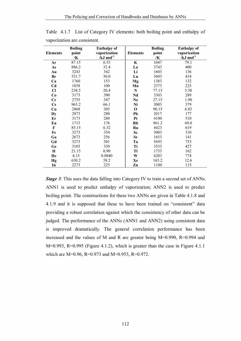
The Policing and Correction of Handbooks and Databases by ANNs
112
Table 4.1.7 List of Category IV elements: both boiling point and enthalpy of
vaporization are consistent.
Elements Boiling point
/K
Enthalpy of vaporization
/kJ mol-1 Elements
Boiling point
/K
Enthalpy of vaporization
/kJ mol-1 Ar 87.15 6.53 K 1047 79.1 As 886.2 32.4 La 3743 400 Au 3243 342 Li 1603 136 Br 331.7 30.0 Lu 3603 414 Ca 1760 153 Mg 1383 132 Cd 1038 100 Mn 2373 225 Cl 238.5 20.4 N 77.15 5.58 Co 3173 390 Nd 3303 289 Cr 2755 347 Ne 27.15 1.90 Cs 963.2 66.1 Ni 3003 379 Cu 2868 305 O 90.15 6.82 Dy 2873 280 Pb 2017 177 Er 3173 280 Pt 4100 510 Eu 1713 176 Rb 961.2 69.0 F 85.15 6.32 Ru 4423 619 Fe 3273 354 Sc 3003 310 Ga 2673 256 Sr 1653 141 Gd 3273 301 Ta 5693 753 Ge 3103 330 Ti 3533 427 H 21.15 0.90 Tl 1733 162 He 4.15 0.0840 W 6203 774 Hg 630.2 58.2 Xe 165.2 12.6 In 2273 225 Zn 1180 115
Stage 3: This uses the data falling into Category IV to train a second set of ANNs.
ANN1 is used to predict enthalpy of vaporization; ANN2 is used to predict
boiling point. The constructions for these two ANNs are given in Table 4.1.8 and
4.1.9 and it is supposed that these to have been trained on “consistent” data
providing a robust correlation against which the consistency of other data can be
judged. The performance of the ANNs (ANN1 and ANN2) using consistent data
is improved dramatically. The general correlation performance has been
increased and the values of M and R are greater being M=0.990, R=0.994 and
M=0.993, R=0.995 (Figure 4.1.2), which is greater than the case in Figure 4.1.1
which are M=0.96, R=0.973 and M=0.953, R=0.972.
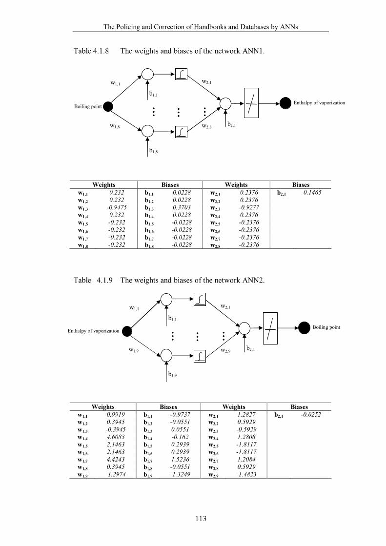
The Policing and Correction of Handbooks and Databases by ANNs
113
Table 4.1.8 The weights and biases of the network ANN1.
Weights Biases Weights Biases
w1,1 0.232 b1,1 0.0228 w2,1 0.2376 b2,1 0.1465 w1,2 0.232 b1,2 0.0228 w2,2 0.2376 w1,3 -0.9475 b1,3 0.3703 w2,3 -0.9277 w1,4 0.232 b1,4 0.0228 w2,4 0.2376 w1,5 -0.232 b1,5 -0.0228 w2,5 -0.2376 w1,6 -0.232 b1,6 -0.0228 w2,6 -0.2376 w1,7 -0.232 b1,7 -0.0228 w2,7 -0.2376 w1,8 -0.232 b1,8 -0.0228 w2,8 -0.2376
Table 4.1.9 The weights and biases of the network ANN2.
Weights Biases Weights Biases w1,1 0.9919 b1,1 -0.9737 w2,1 1.2827 b2,1 -0.0252 w1,2 0.3945 b1,2 -0.0551 w2,2 0.5929 w1,3 -0.3945 b1,3 0.0551 w2,3 -0.5929 w1,4 4.6083 b1,4 -0.162 w2,4 1.2808 w1,5 2.1463 b1,5 0.2939 w2,5 -1.8117 w1,6 2.1463 b1,6 0.2939 w2,6 -1.8117 w1,7 4.4243 b1,7 1.5236 w2,7 1.2084 w1,8 0.3945 b1,8 -0.0551 w2,8 0.5929 w1,9 -1.2974 b1,9 -1.3249 w2,9 -1.4823
Enthalpy of vaporization Boiling point
w2,8
w2,1
b2,1
…
w1,1
b1,1
…
b1,8
w1,8
…
Enthalpy of vaporization Boiling point
w2,9
w2,1
b2,1
…
w1,1 b1,1
…
b1,9
w1,9
…
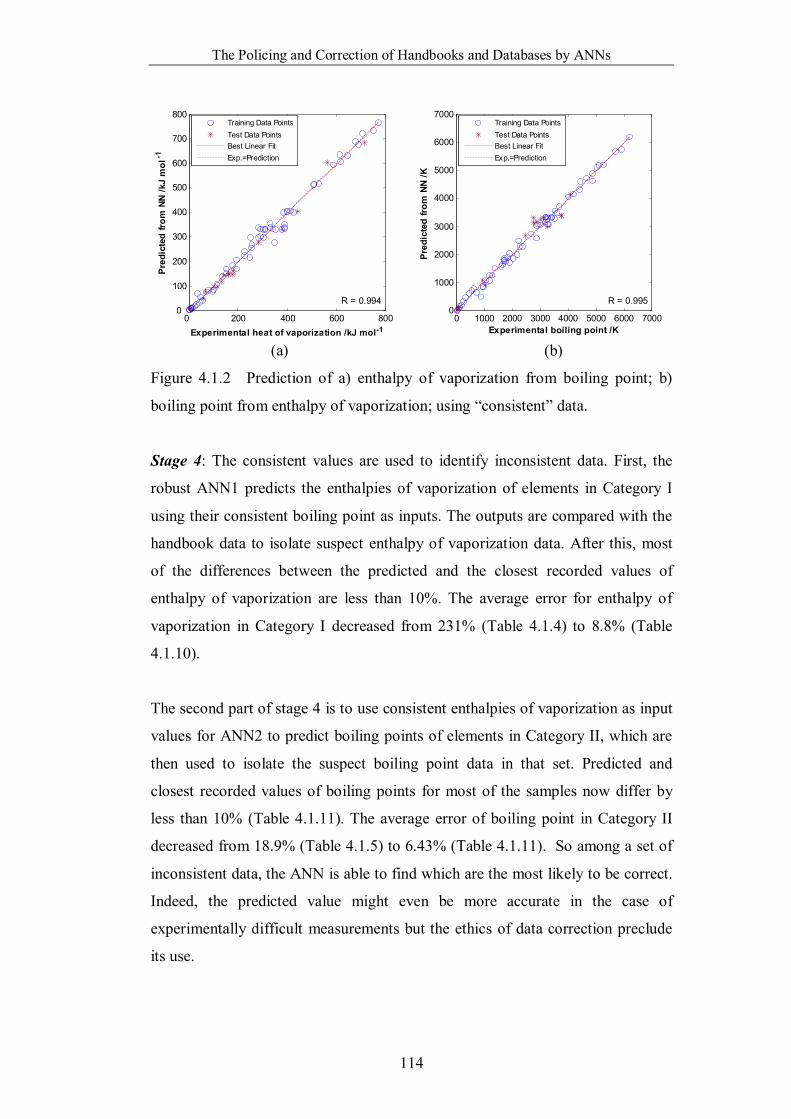
The Policing and Correction of Handbooks and Databases by ANNs
114
0 200 400 600 8000
100
200
300
400
500
600
700
800
Experimental heat of vaporization /kJ mol-1
Pred
icte
d fro
m N
N /k
J m
ol-1
R = 0.994
Training Data PointsTest Data PointsBest Linear FitExp.=Prediction
0 1000 2000 3000 4000 5000 6000 7000
0
1000
2000
3000
4000
5000
6000
7000
Experimental boiling point /K
Pred
icte
d fro
m N
N /K
R = 0.995
Training Data PointsTest Data PointsBest Linear FitExp.=Prediction
(a) (b)
Figure 4.1.2 Prediction of a) enthalpy of vaporization from boiling point; b)
boiling point from enthalpy of vaporization; using “consistent” data.
Stage 4: The consistent values are used to identify inconsistent data. First, the
robust ANN1 predicts the enthalpies of vaporization of elements in Category I
using their consistent boiling point as inputs. The outputs are compared with the
handbook data to isolate suspect enthalpy of vaporization data. After this, most
of the differences between the predicted and the closest recorded values of
enthalpy of vaporization are less than 10%. The average error for enthalpy of
vaporization in Category I decreased from 231% (Table 4.1.4) to 8.8% (Table
4.1.10).
The second part of stage 4 is to use consistent enthalpies of vaporization as input
values for ANN2 to predict boiling points of elements in Category II, which are
then used to isolate the suspect boiling point data in that set. Predicted and
closest recorded values of boiling points for most of the samples now differ by
less than 10% (Table 4.1.11). The average error of boiling point in Category II
decreased from 18.9% (Table 4.1.5) to 6.43% (Table 4.1.11). So among a set of
inconsistent data, the ANN is able to find which are the most likely to be correct.
Indeed, the predicted value might even be more accurate in the case of
experimentally difficult measurements but the ethics of data correction preclude
its use.
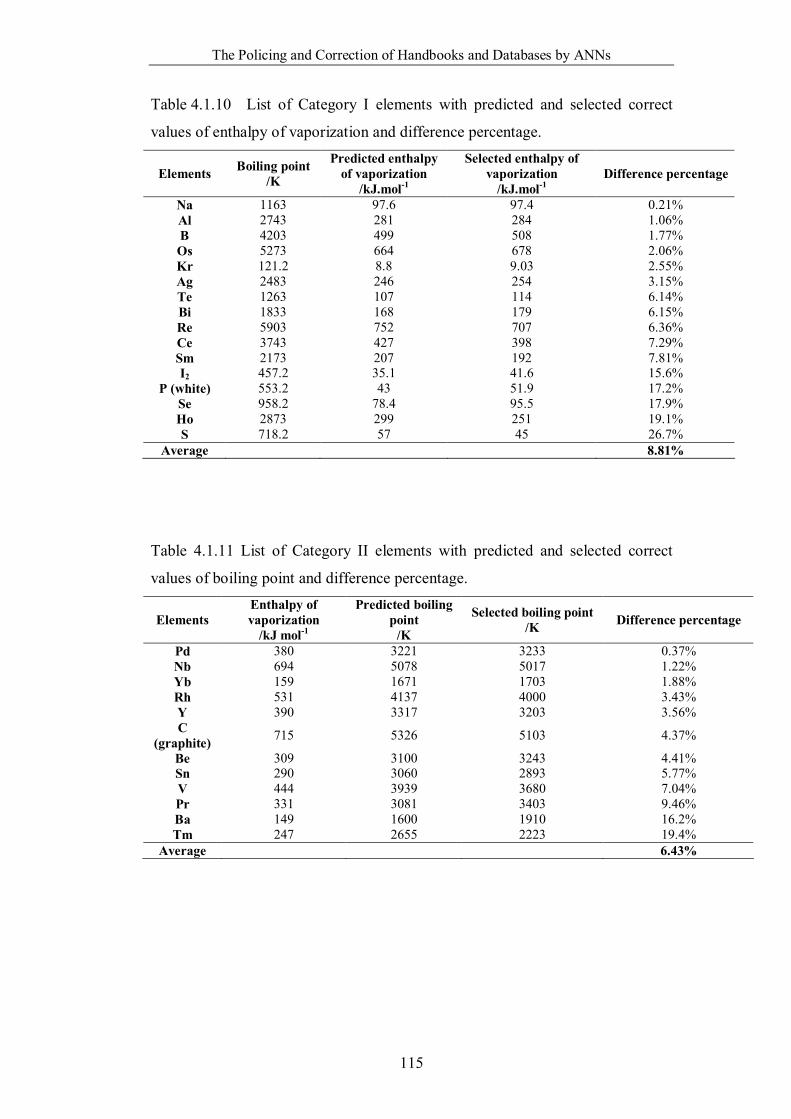
The Policing and Correction of Handbooks and Databases by ANNs
115
Table 4.1.10 List of Category I elements with predicted and selected correct
values of enthalpy of vaporization and difference percentage.
Elements Boiling point /K
Predicted enthalpy of vaporization
/kJ.mol-1
Selected enthalpy of vaporization
/kJ.mol-1 Difference percentage
Na 1163 97.6 97.4 0.21% Al 2743 281 284 1.06% B 4203 499 508 1.77% Os 5273 664 678 2.06% Kr 121.2 8.8 9.03 2.55% Ag 2483 246 254 3.15% Te 1263 107 114 6.14% Bi 1833 168 179 6.15% Re 5903 752 707 6.36% Ce 3743 427 398 7.29% Sm 2173 207 192 7.81% I2 457.2 35.1 41.6 15.6%
P (white) 553.2 43 51.9 17.2% Se 958.2 78.4 95.5 17.9% Ho 2873 299 251 19.1% S 718.2 57 45 26.7%
Average 8.81%
Table 4.1.11 List of Category II elements with predicted and selected correct
values of boiling point and difference percentage.
Elements Enthalpy of vaporization
/kJ mol-1
Predicted boiling point
/K
Selected boiling point /K Difference percentage
Pd 380 3221 3233 0.37% Nb 694 5078 5017 1.22% Yb 159 1671 1703 1.88% Rh 531 4137 4000 3.43% Y 390 3317 3203 3.56% C
(graphite) 715 5326 5103 4.37%
Be 309 3100 3243 4.41% Sn 290 3060 2893 5.77% V 444 3939 3680 7.04% Pr 331 3081 3403 9.46% Ba 149 1600 1910 16.2% Tm 247 2655 2223 19.4%
Average 6.43%
The Policing and Correction of Handbooks and Databases by ANNs
116
The data in Category III are treated as follows. It is supposed that if one of the
inconsistent values in one property is correct, it might be used to predict a value
close to one of the inconsistent values in the other property. For example, for Si,
it has a very wide range of handbook boiling points of 2633 K, 2628 K, 3533 K
and 3538 K and handbook enthalpies of vaporization of 300, 359 and 383 kJ/mol.
So its possible boiling points were predicted using all three enthalpies of
vaporization and ANN2 obtaining 3091K, 3096 K, and 3250 K respectively. The
differences of predicted boiling points with handbook data can be calculated (12
different combinations). The minimum difference is 8 % between 3533 K
(handbook) and 3250 K (predicted from enthalpy of vaporization 383 kJ/mol). So
a possible pair is obtained: 3533 K and 383 kJ/mol. Then the ANN1 was used to
predict possible enthalpies of vaporization using four handbook boiling points,
giving another 12 combinations. The minimum difference corresponds to the pair
3533 K and 383 kJ/mol again (predicted enthalpy of vaporization 395 kJ/mol
gives a 3% difference with 383 kJ/mol). This points to the correct boiling point
of Si as 3533 K and enthalpy of vaporization, 383 kJ/mol.
The case of silicon may have been lucky – the same pair was obtained in both
prediction directions and identification is easily. In some cases the pairs are
different in different prediction directions. For iridium, the two pairs are 4701 K
and 564 kJ/mol, and 4403 K and 636 kJ/mol. In the first pair, the predicted
enthalpy of vaporization is 577 kJ/mol (2.4% difference from 564 kJ/mol)
predicted from 4701 K. But in the reverse direction, the prediction of boiling
point from 564 kJ/mol is 4158 K, which has 12% difference with 4701 K. In the
second pair, the predicted boiling point 4510 K has the smallest difference with
4403 K (2.4%), but in the reverse direction, the difference is 16.6%. It is difficult
to point out which pair is more favourable and it looks as though a lengthy
indagation of the original sources is inevitable; a quest made problematic
because many handbooks are now silent about sources. There is however one
other trick that sometimes works.
In such cases, a comprehensive minimum of difference can be calculated. For the
general situation, m boiling points Boi (i=1,2…m), and n enthalpies of
vaporization Hoj (j=1,2…n) from handbooks are available. The ANN will predict
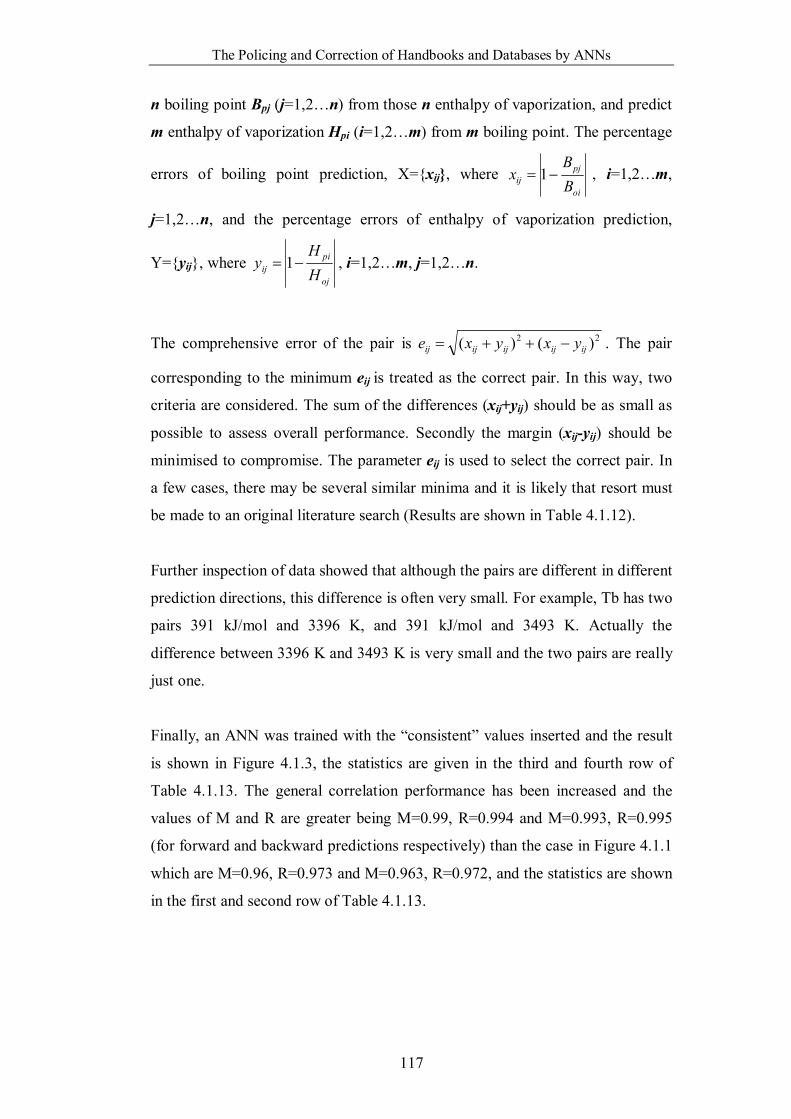
The Policing and Correction of Handbooks and Databases by ANNs
117
n boiling point Bpj (j=1,2…n) from those n enthalpy of vaporization, and predict
m enthalpy of vaporization Hpi (i=1,2…m) from m boiling point. The percentage
errors of boiling point prediction, X={xij}, where oi
pjij B
Bx 1 , i=1,2…m,
j=1,2…n, and the percentage errors of enthalpy of vaporization prediction,
Y={yij}, where oj
piij H
Hy 1 , i=1,2…m, j=1,2…n.
The comprehensive error of the pair is 22 )()( ijijijijij yxyxe . The pair
corresponding to the minimum eij is treated as the correct pair. In this way, two
criteria are considered. The sum of the differences (xij+yij) should be as small as
possible to assess overall performance. Secondly the margin (xij-yij) should be
minimised to compromise. The parameter eij is used to select the correct pair. In
a few cases, there may be several similar minima and it is likely that resort must
be made to an original literature search (Results are shown in Table 4.1.12).
Further inspection of data showed that although the pairs are different in different
prediction directions, this difference is often very small. For example, Tb has two
pairs 391 kJ/mol and 3396 K, and 391 kJ/mol and 3493 K. Actually the
difference between 3396 K and 3493 K is very small and the two pairs are really
just one.
Finally, an ANN was trained with the “consistent” values inserted and the result
is shown in Figure 4.1.3, the statistics are given in the third and fourth row of
Table 4.1.13. The general correlation performance has been increased and the
values of M and R are greater being M=0.99, R=0.994 and M=0.993, R=0.995
(for forward and backward predictions respectively) than the case in Figure 4.1.1
which are M=0.96, R=0.973 and M=0.963, R=0.972, and the statistics are shown
in the first and second row of Table 4.1.13.
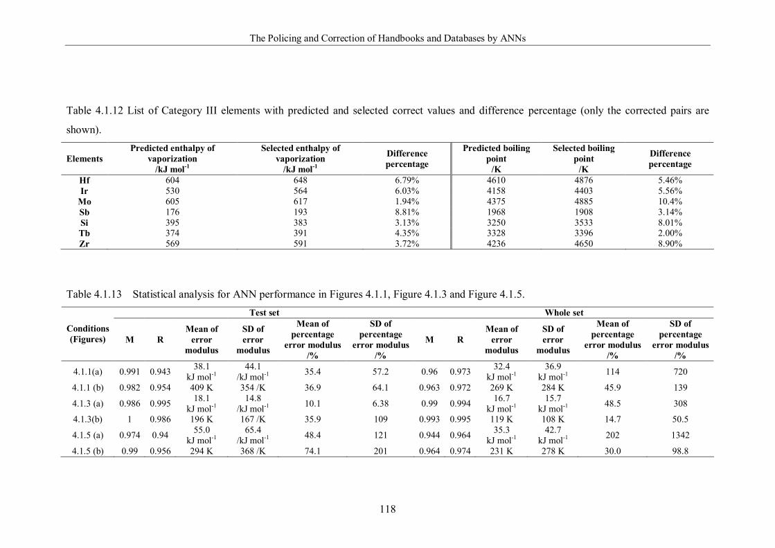
The Policing and Correction of Handbooks and Databases by ANNs
118
Table 4.1.12 List of Category III elements with predicted and selected correct values and difference percentage (only the corrected pairs are
shown).
Elements Predicted enthalpy of
vaporization /kJ mol-1
Selected enthalpy of vaporization
/kJ mol-1
Difference percentage
Predicted boiling point
/K
Selected boiling point
/K
Difference percentage
Hf 604 648 6.79% 4610 4876 5.46% Ir 530 564 6.03% 4158 4403 5.56%
Mo 605 617 1.94% 4375 4885 10.4% Sb 176 193 8.81% 1968 1908 3.14% Si 395 383 3.13% 3250 3533 8.01% Tb 374 391 4.35% 3328 3396 2.00% Zr 569 591 3.72% 4236 4650 8.90%
Table 4.1.13 Statistical analysis for ANN performance in Figures 4.1.1, Figure 4.1.3 and Figure 4.1.5. Test set Whole set
Conditions (Figures) M R
Mean of error
modulus
SD of error
modulus
Mean of percentage
error modulus /%
SD of percentage
error modulus /%
M R Mean of
error modulus
SD of error
modulus
Mean of percentage
error modulus /%
SD of percentage
error modulus /%
4.1.1(a) 0.991 0.943 38.1 kJ mol-1
44.1 /kJ mol-1 35.4 57.2 0.96 0.973 32.4
kJ mol-1 36.9
kJ mol-1 114 720
4.1.1 (b) 0.982 0.954 409 K 354 /K 36.9 64.1 0.963 0.972 269 K 284 K 45.9 139
4.1.3 (a) 0.986 0.995 18.1 kJ mol-1
14.8 /kJ mol-1 10.1 6.38 0.99 0.994 16.7
kJ mol-1 15.7
kJ mol-1 48.5 308
4.1.3(b) 1 0.986 196 K 167 /K 35.9 109 0.993 0.995 119 K 108 K 14.7 50.5
4.1.5 (a) 0.974 0.94 55.0 kJ mol-1
65.4 /kJ mol-1 48.4 121 0.944 0.964 35.3
kJ mol-1 42.7
kJ mol-1 202 1342
4.1.5 (b) 0.99 0.956 294 K 368 /K 74.1 201 0.964 0.974 231 K 278 K 30.0 98.8

The Policing and Correction of Handbooks and Databases by ANNs
119
4.3 Discussion
4.3.1 Comparisons of ANN Curves
In this work, error detection and correction is based on the binary correlation
between properties, so it is possible to interpret the results visually by drawing a
2-D diagram. The interpretation is shown in Figure 4.1.4, which is constructed as
follows:
1. The boiling point is placed on the abscissa and enthalpy of vaporization
on the ordinate for both ANNs.
2. The data in Category IV are plotted directly and are shown as blue dots.
For these data, the boiling point values are within the range 0 K –7000 K;
while the enthalpy of vaporization values are within the range 0 kJ mol-1–
800 kJ mol-1.
3. The ANN1 was fed with artificial boiling point data from 0 to 7000
(taking 1 as interval) to predict corresponding enthalpy of vaporization.
Those data were used to draw a complete curve 1. This curve is shown as
the green dot-dash line.
4. Similarly, the ANN2 was fed with artificial enthalpy of vaporization
prediction from 0 to 800 (taking 0.02 as interval) to predict the
corresponding boiling point. These data were used to draw curve 2. This
curve is shown as a red solid line.
5. The data in Category IV have up to 10% variation between minimum and
maximum values so it is reasonable to put ±10% bounds for each curve to
show the uncertainty of the prediction. For curve 1, the enthalpy of
vaporization was multiplied by 110% and 90%, and for curve 2, the
boiling point was multiplied by 110% and 90%. The boundaries are
shown as green or red dotted lines.
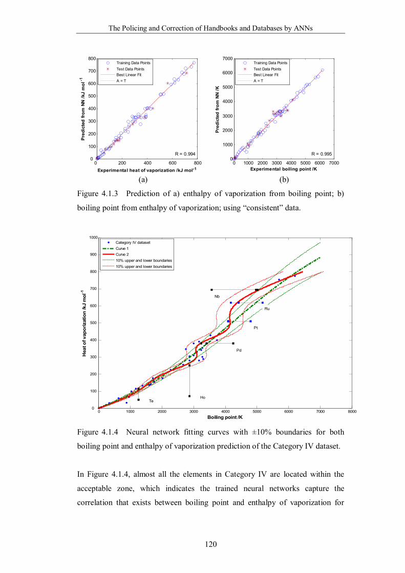
The Policing and Correction of Handbooks and Databases by ANNs
120
0 200 400 600 8000
100
200
300
400
500
600
700
800
Experimental heat of vaporization /kJ mol-1
Pred
icte
d fro
m N
N /k
J m
ol-1
R = 0.994
Training Data PointsTest Data PointsBest Linear FitA = T
0 1000 2000 3000 4000 5000 6000 7000
0
1000
2000
3000
4000
5000
6000
7000
Experimental boiling point /K
Pred
icte
d fro
m N
N /K
R = 0.995
Training Data PointsTest Data PointsBest Linear FitA = T
(a) (b)
Figure 4.1.3 Prediction of a) enthalpy of vaporization from boiling point; b)
boiling point from enthalpy of vaporization; using “consistent” data.
0 1000 2000 3000 4000 5000 6000 7000 80000
100
200
300
400
500
600
700
800
900
1000
Boiling point /K
Hea
t of v
apor
izat
ion
/kJ
mol
-1
Category IV datasetCurve 1Curve 210% upper and lower boundaries10% upper and lower boundaries
Ho
Pd
Nb
Te
Ru
Pt
Figure 4.1.4 Neural network fitting curves with ±10% boundaries for both
boiling point and enthalpy of vaporization prediction of the Category IV dataset.
In Figure 4.1.4, almost all the elements in Category IV are located within the
acceptable zone, which indicates the trained neural networks capture the
correlation that exists between boiling point and enthalpy of vaporization for
The Policing and Correction of Handbooks and Databases by ANNs
121
Category IV elements. This enhanced the confidence in using the trained network
derived from stage 3 to identify inconsistent data in stage 4.
If the ideal equation between enthalpy of vaporization and boiling point was
found by the ANN then curves 1 and 2 should be identical. However, curves 1
and 2 are different in shape and this means the neural networks found two
different equations to represent the correlation between boiling point and
enthalpy of vaporization. The reasons for that could be a) noise from the data; b)
other unknown properties influence enthalpy of vaporization and/or boiling point.
As a result, the neural network cannot find an exact function but a correlation. It
minimizes the estimate uncertainty of one quantity, when given a value for the
other. The uncertainty makes the two curves different.
Although the ANN found that curve 1 is the best prediction for enthalpy of
vaporization, it is interesting to test whether curve 2 performs better on the
prediction of enthalpy of vaporization; and vice versa. Here, the sum of the
squared residuals (SSE) in both boiling point and enthalpy of vaporization for
each curve were used as a criterion, which is the same criterion used in
regression analysis. When curve 1 is used to predict the enthalpy of vaporization,
the sum of the squares of discrepancies is 3.75×10⁴ kJ2 mol-2, and when curve 2
is used to do the same prediction, the value is 5.75×10⁴ kJ2 mol-2. Similar, when
the curve 2 is used to predict the boiling point, the value is 1.02×10⁶ K2 and
when curve 1 is used, the value is 1.99×10⁶ K2.
From comparison of these values, it can be found that for enthalpy of
vaporization, the SSE calculated from curve 1 is smaller, but not significantly so,
than the value calculated from curve 2; and for boiling point, the SSE calculated
from curve 2 is smaller, but not significantly so, than the value calculated from
curve 1. As the result, it can be said curve 1 is better for predicting the enthalpy
of vaporization, and curve 2 is better for predicting the boiling point, and the
neural network found the right one for each. Also, from the comparison made
above, the difference in each case is not great, which suggests both of the fitting
curves are sensible.
The Policing and Correction of Handbooks and Databases by ANNs
122
To illustrate the relationship between the curve and the inconsistent data, the data
of some elements were drawn in Figure 4.1.4. Clearly, the correct values should
be the points close to the curves.
4.3.2 Measurement Methods for Boiling Points and Enthalpy of
Vaporization
It is important to remember that these two properties are not directly related.
They are based on the Clausius-Clapeyron equation: that is
vvp
v
v
vvp
ZPRTH
VTH
dTdP
)/( 2 , which in its integrated form gives,
RTHiP v
vp exp . The boiling point is the temperature at which Pvp reaches
ambient but the pre-exponential coefficient is not included in the ANN making
the relationship indirect.
Boiling point is the temperature at which the vapour pressure of a liquid is equal
to the external pressure; and when the external pressure equals 1 atmosphere, the
boiling point is called the normal boiling point, which is the meaning in this
work.
The enthalpy of vaporization of materials is not a property which can be
measured directly as can boiling point. In Poling et al.’s book (2000), three
categories of method to estimate the enthalpy of vaporization are summarised: 1)
Based on the Clausius-Clapeyron equation vvp
v
v
vvp
ZPRTH
VTH
dTdP
)/( 2 ,
dTdPvp
is found from a vapour-pressure temperature correlation, and then vH can be
obtained after the estimation of vZ , which is the difference in compressibility
factor of saturated vapour and saturated liquid; 2) Use of the principle of
corresponding states to make the estimation, such as the equations developed by
Pitzer et al. (1955), Fish and Lielmezs (1975), Nath (1979), Sivaraman et al.
(1984), Meyra et al. (2004), Malagoni et al. (2005), Cachadiña and Mulero
(2007); 3) In the case of estimating vH from normal boiling point, there are
some additional techniques available, such as Giacalone’s equation which was
The Policing and Correction of Handbooks and Databases by ANNs
123
first developed in 1951 and with improved accuracy by Fishtine and Klein
(Poling et al., 2000), the Riedel method (1954), McCurdy and Laidler (1963),
the Chen method (1965), the Vetere method (1973), and also some others done
by Fedors (1974), Lawson (1980), Guthrie and Taylor (1983), Hoshino et al.
(1983), Ma and Zhao (1993), Constantinou and Gani (1994), Tu and Liu (1996).
For most of the correlations in these three categories, critical constants Tc and Pc
are required either directly or indirectly. As a result, it is reasonable to say that
there is a correlation, which is a confounding association, between the boiling
point and enthalpy of vaporization, although the function is not known exactly.
This is an example of the situation in which the ANN can be applied.
4.3.3 Original Sources of Property Values
To verify the method, original sources were consulted where possible 1) to check
whether the refined values were sensible, 2) to reveal and analyse the origin of
the differences between handbook data and 3) to find whether the neural network
can give values closer to the original literature. Representative examples are
shown below. Some errors are attributable to incorrect unit conversions, some to
different reference conditions.
Table 4.1.10 indicates that predicted and closest recorded values of enthalpy of
vaporization for most elements differ by less than 10% after removal of incorrect
data. The exceptions are I2 (15.5%), P (17.1%), Se (17.9%), Ho (19.0%) and S
(26.7%). Data for elements I2, P and S depend on the polyatomic nature of these
molecules and this accounts for the differences as shown in Table 4.1.3 but
handbooks do not always state how the value is normalised. In these cases, where
the substances always exist in their molecular forms, the corresponding enthalpy
of vaporization should be accounted for molecular form. From Table 4.1.10, the
corrected values are reasonable choices, although the differences are still greater
than 10%. The detailed investigations of Ho and Se are shown below. These
results show that the ANNs can predict more reliable data.
The Policing and Correction of Handbooks and Databases by ANNs
124
For holmium (Ho), there are two sources of discrepancy. Original sources for
stvH , offer 71910 cal mol-1 (Hultgren et al., 1973), 69500 cal mol-1 (White et
al., 1961), 75040 cal mol-1 (Trulson et al., 1961), 81150 cal mol-1 (Hultgren et
al., 1973) and 70600 cal mol-1 (Wakefield et al., 1967). Clearly these results
indicate the enthalpy of vaporization of holmium is around 71 kcal mol-1,
corresponding to 297 kJ mol-1, rather than the 71 kJ mol-1 recorded in Lange’s
Handbook of Chemistry and the source of error is transcription of units. Indeed in
the earlier 12th edition of Lange’s Handbook Chemistry (Dean, 1979), the value
was 60 kcal mol-1, placing it in the correct range.
The selected handbook value of 251 kJ mol-1 still differs by more than 10% from
the ANN predicted value of 299 kJ mol-1. The second source of discrepancy is
the reference temperature. All the above values are corrected to standard
temperature. However the Category IV values used for training ANNs 1 and 2
are all referenced to normal boiling point (with the exception of four elements).
Values for the enthalpy of vaporization of Ho at normal boiling point are
available: 67 kJ mol-1 corresponding to 280 kJ mol-1 (Daane, 1961) and 64.7 1molcal corresponding to 270 kJ mol-1 (Wakefield et al., 1967). These values
are close to the value predicted by the ANN and this demonstrates the
remarkable discernment of the ANN in detection of errors and identification of
true values.
The case of selenium is different. The handbook values are 14, 26.3 and 95.5 kJ
mol-1 and the ANN predicts 78.4 kJ mol-1 from the well-established boiling point
of 958 K (as a fixed point in International Temperature Scale) (De Selincourt,
1940; Brooks, 1952). The source for 95.5 kJ mol-1 can be found (Brooks, 1952),
in which Brooks used the Bourdon gage method and Clapeyron equation
TBAPVP ln , and determined the enthalpy of vaporization for Se at the normal
boiling point which is 22.02 ± 0.02 kcal/mol and corresponds to 95.48 ± 0.08
kJ/mol. This is supported by Hutlgren et al. (1973) who gives a value at 625 K
where, of the eight chemical allotropes for gaseous Se, Se6 predominates
(Bagnall, 1966). The value of 13.8 kJ mol-1 for atomic Se corresponds to 82.8 kJ
The Policing and Correction of Handbooks and Databases by ANNs
125
mol-1 for Se6 (Hultgren et al., 1973). This may explain the handbook value of 14
kJ mol-1, if that value be for atomic Se. The handbook value of 26.3 kJ mol-1
begins to look like a transcription of units error of x4.18 J cal-1. The selected
value of 95.5 kJ mol-1 still deviates by more than 10% from the ANN predicted
value 78.4 kJ mol-1. A possible reason for this, as discussed by Bagnall (1966)
and Reid et al. (1987), is associated with constants in the Clapeyron equation and
is described in the part 4.3.5.
4.3.4 Comparison with the Method used by Ashby
The ANN technique was also used to double-check the statistical approach
(Ashby, 1998; Bassetti et al., 1998) used for CES software (previously
Cambridge Materials Selector, CMS). The CES data was used to train an ANN
and it gave correlation coefficients of 0.964 and 0.974 compared with 0.994 and
0.995 when using the “consistent” data (shown in Figure 4.1.5, and statistical
analysis as shown in fifth and sixth row of Table 4.1.13). For example, consider
the enthalpy of vaporization for Se. The value taken from CES Software is 207
kJ mol-1 but other sources give 14, 26.3 and 95.5 kJ mol-1. The value for enthalpy
of vaporization for phosphorous (P, white) in CES software is 316 kJ mol-1,
while the values quoted by Dainton and Kimberley (1950) and other sources is
12.4 kJ mol-1 for ¼ P4 or 51.9 kJ mol-1 for P4. These are large discrepancies for
elemental data.
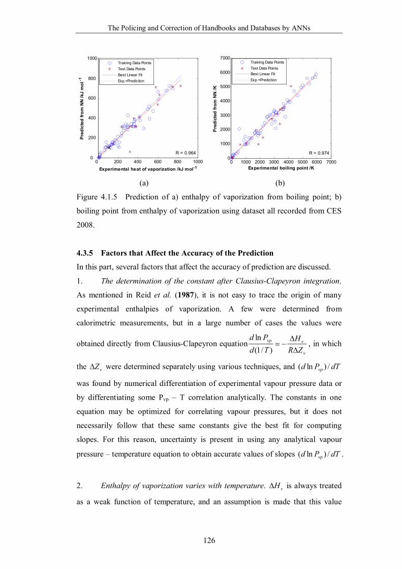
The Policing and Correction of Handbooks and Databases by ANNs
126
0 200 400 600 800 10000
200
400
600
800
1000
Experimental heat of vaporization /kJ mol-1
Pred
icte
d fro
m N
N /k
J m
ol-1
R = 0.964
K
Training Data PointsTest Data PointsBest Linear FitExp.=Prediction
0 1000 2000 3000 4000 5000 6000 7000
0
1000
2000
3000
4000
5000
6000
7000
Experimental boiling point /K
Pre
dict
ed fr
om N
N /K
R = 0.974
Training Data PointsTest Data PointsBest Linear FitExp.=Prediction
(a) (b)
Figure 4.1.5 Prediction of a) enthalpy of vaporization from boiling point; b)
boiling point from enthalpy of vaporization using dataset all recorded from CES
2008.
4.3.5 Factors that Affect the Accuracy of the Prediction
In this part, several factors that affect the accuracy of prediction are discussed.
1. The determination of the constant after Clausius-Clapeyron integration.
As mentioned in Reid et al. (1987), it is not easy to trace the origin of many
experimental enthalpies of vaporization. A few were determined from
calorimetric measurements, but in a large number of cases the values were
obtained directly from Clausius-Clapeyron equationv
vvp
ZRH
TdPd
)/1(
ln, in which
the vZ were determined separately using various techniques, and dTPd vp /)ln(
was found by numerical differentiation of experimental vapour pressure data or
by differentiating some Pvp – T correlation analytically. The constants in one
equation may be optimized for correlating vapour pressures, but it does not
necessarily follow that these same constants give the best fit for computing
slopes. For this reason, uncertainty is present in using any analytical vapour
pressure – temperature equation to obtain accurate values of slopes dTPd vp /)ln( .
2. Enthalpy of vaporization varies with temperature. vH is always treated
as a weak function of temperature, and an assumption is made that this value
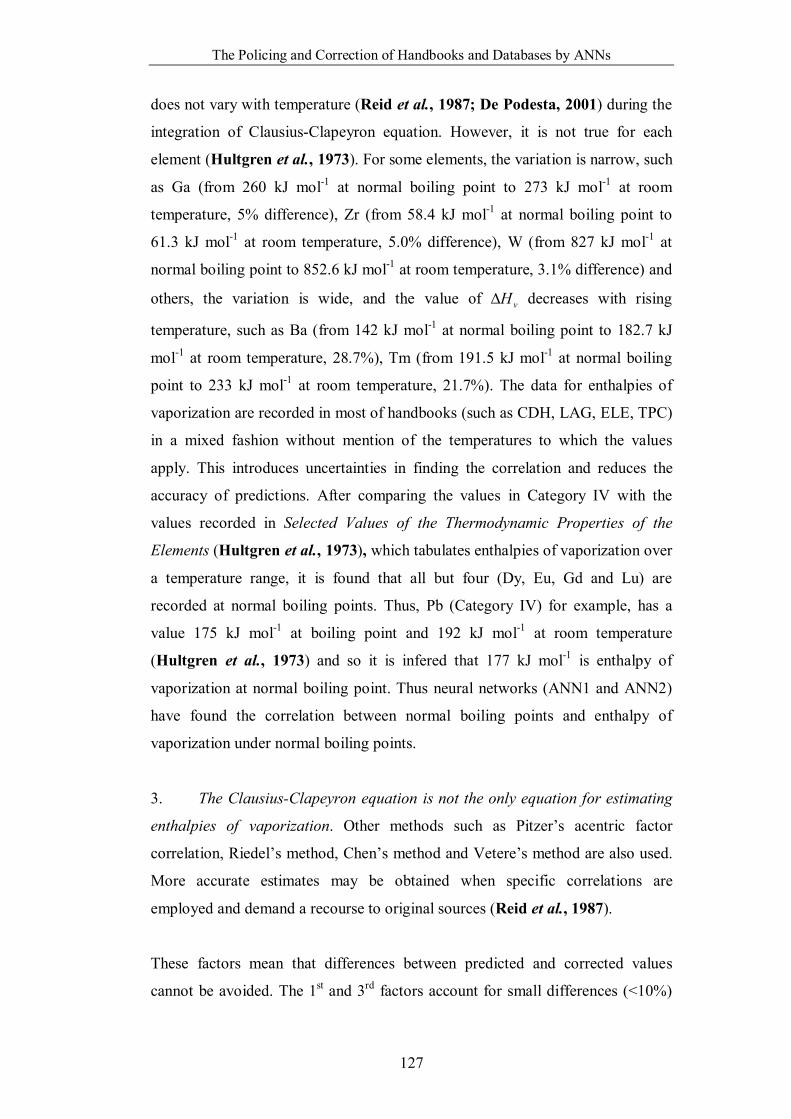
The Policing and Correction of Handbooks and Databases by ANNs
127
does not vary with temperature (Reid et al., 1987; De Podesta, 2001) during the
integration of Clausius-Clapeyron equation. However, it is not true for each
element (Hultgren et al., 1973). For some elements, the variation is narrow, such
as Ga (from 260 kJ mol-1 at normal boiling point to 273 kJ mol-1 at room
temperature, 5% difference), Zr (from 58.4 kJ mol-1 at normal boiling point to
61.3 kJ mol-1 at room temperature, 5.0% difference), W (from 827 kJ mol-1 at
normal boiling point to 852.6 kJ mol-1 at room temperature, 3.1% difference) and
others, the variation is wide, and the value of vH decreases with rising
temperature, such as Ba (from 142 kJ mol-1 at normal boiling point to 182.7 kJ
mol-1 at room temperature, 28.7%), Tm (from 191.5 kJ mol-1 at normal boiling
point to 233 kJ mol-1 at room temperature, 21.7%). The data for enthalpies of
vaporization are recorded in most of handbooks (such as CDH, LAG, ELE, TPC)
in a mixed fashion without mention of the temperatures to which the values
apply. This introduces uncertainties in finding the correlation and reduces the
accuracy of predictions. After comparing the values in Category IV with the
values recorded in Selected Values of the Thermodynamic Properties of the
Elements (Hultgren et al., 1973), which tabulates enthalpies of vaporization over
a temperature range, it is found that all but four (Dy, Eu, Gd and Lu) are
recorded at normal boiling points. Thus, Pb (Category IV) for example, has a
value 175 kJ mol-1 at boiling point and 192 kJ mol-1 at room temperature
(Hultgren et al., 1973) and so it is infered that 177 kJ mol-1 is enthalpy of
vaporization at normal boiling point. Thus neural networks (ANN1 and ANN2)
have found the correlation between normal boiling points and enthalpy of
vaporization under normal boiling points.
3. The Clausius-Clapeyron equation is not the only equation for estimating
enthalpies of vaporization. Other methods such as Pitzer’s acentric factor
correlation, Riedel’s method, Chen’s method and Vetere’s method are also used.
More accurate estimates may be obtained when specific correlations are
employed and demand a recourse to original sources (Reid et al., 1987).
These factors mean that differences between predicted and corrected values
cannot be avoided. The 1st and 3rd factors account for small differences (<10%)
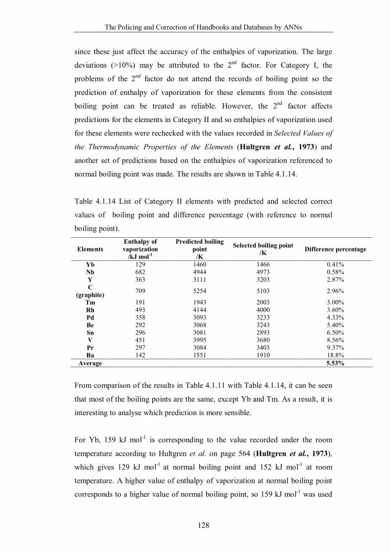
The Policing and Correction of Handbooks and Databases by ANNs
128
since these just affect the accuracy of the enthalpies of vaporization. The large
deviations (>10%) may be attributed to the 2nd factor. For Category I, the
problems of the 2nd factor do not attend the records of boiling point so the
prediction of enthalpy of vaporization for these elements from the consistent
boiling point can be treated as reliable. However, the 2nd factor affects
predictions for the elements in Category II and so enthalpies of vaporization used
for these elements were rechecked with the values recorded in Selected Values of
the Thermodynamic Properties of the Elements (Hultgren et al., 1973) and
another set of predictions based on the enthalpies of vaporization referenced to
normal boiling point was made. The results are shown in Table 4.1.14.
Table 4.1.14 List of Category II elements with predicted and selected correct
values of boiling point and difference percentage (with reference to normal
boiling point).
Elements Enthalpy of vaporization
/kJ mol-1
Predicted boiling point
/K
Selected boiling point /K Difference percentage
Yb 129 1460 1466 0.41% Nb 682 4944 4973 0.58% Y 363 3111 3203 2.87% C
(graphite) 709 5254 5103 2.96%
Tm 191 1943 2003 3.00% Rh 493 4144 4000 3.60% Pd 358 3093 3233 4.33% Be 292 3068 3243 5.40% Sn 296 3081 2893 6.50% V 451 3995 3680 8.56% Pr 297 3084 3403 9.37% Ba 142 1551 1910 18.8%
Average 5.53%
From comparison of the results in Table 4.1.11 with Table 4.1.14, it can be seen
that most of the boiling points are the same, except Yb and Tm. As a result, it is
interesting to analyse which prediction is more sensible.
For Yb, 159 kJ mol-1 is corresponding to the value recorded under the room
temperature according to Hultgren et al. on page 564 (Hultgren et al., 1973),
which gives 129 kJ mol-1 at normal boiling point and 152 kJ mol-1 at room
temperature. A higher value of enthalpy of vaporization at normal boiling point
corresponds to a higher value of normal boiling point, so 159 kJ mol-1 was used

The Policing and Correction of Handbooks and Databases by ANNs
129
to predict boiling point giving the higher value of boiling point for Yb. Two
factors need to be considered: 1) For different elements, those having higher
normal boiling points always have higher enthalpies of vaporization at the
normal boiling point; 2) For a given element, the enthalpy of vaporization varies
inversely with temperature. For Yb, the boiling point is higher than ambient and
so the enthalpy of vaporization at boiling point is lower than the value at
ambience. Previously, the enthalpy of vaporization at room temperature was used
to predict boiling point, and the first factor means the boiling point was over-
estimated. Now the enthalpy of vaporization at normal boiling point is employed
and the boiling point prediction is correct. Using 129 kJ mol-1, the corresponding
boiling point is 1460 K, which is closer to 1466 K (within 0.40%), and this value
is confirmed by the work of Habermann and Daane (Habermann and Daane,
1964). In their work, the vapour pressures of the rare-earth metals were measured
by the Knudsen effusion technique using a quartz-fibre microbalance, and then a
combination of Second and Third Law methods were used to calculate the
normal boiling point for each rare-earth metal, and for Yb this value is 1466
(±5)K.
For Tm, 247 kJ mol-1 is the value corresponding to ambient temperature,
according to Hultgren et al. on page 533 (Hultgren et al., 1973), which gives
191 kJ mol-1 at normal boiling point and 232 kJ mol-1 at room temperature and is
greater than the value recorded at normal boiling point which is about 191 kJ
mol-1. For similar reasons, 247 kJ mol-1 was used to predict boiling point
producing a higher value. Using the value of 191 kJ mol-1, it is found the boiling
point is 1943 K, which is closer to 2003K (within 3.00%), and is consistent with
the value obtained by Spedding et al. after purifying this element at the Ames
Laboratory of the U. S. Atomic Energy Commission (Spedding et al., 1957),
which was 2000 K.
From this analysis, the prediction of boiling point in these cases is more
justifiable, than before. So it emerges that although there are several factors,
especially the 2nd, that may mislead the neural network method, when care is
taken and critical surveys are employed, it turns out to be robust and reliable.
The Policing and Correction of Handbooks and Databases by ANNs
130
4.3.6 The Generality and Limitations of This Method
Generality
In a general situation, there may be more than two properties correlated. All that
is required is sufficient correlation, as established by the ANN, to give
demarcation between a majority of well correlated data-points and an outlying
minority. If more than two properties are correlated, a similar procedure can also
be applied. In the following, the mathematical expressions for use when three
properties are correlated and given. The situation for more properties is derived
by analogy with this.
The first step is to find a database of consistent records of all three properties
(Category I in Table 4.1.15). Those data will be used to train three ANNs (i.e.,
ANN1, the prediction of C using A and B, ANN2, the prediction of B using A
and C, and ANN3, the prediction of A using B and C). The other records are
classified into categories 2-8 according to the number of inconsistent properties.
Table 4.1.15 Systematic methodology for error checking in handbooks. Categories A B C Methodology
1 1 1 1 Used to train three ANNs. 2 1 1 0 3 1 0 1 4 0 1 1
Method 1
5 0 0 1 6 0 1 0 7 1 0 0
Method 2
8 0 0 0 Method 3
1 = property records are consistent in different handbooks
0 = property records are inconsistent in different handbooks
The Methods 1, 2 and 3 listed in Table 4.1.15 can be described as follows:
Method 1: Take Category 2 as an example. Inconsistent properties C can be
predicted directly from properties A and B by using ANN1.
The Policing and Correction of Handbooks and Databases by ANNs
131
Method 2: Take Category 5 as an example. For a general situation, we may have
l records of property A {A(o)i, i = 1, 2, … l}, m records of property B {B(o)j, j = 1,
2, … m) from handbooks.
The ANN3 will predict m property A {A(p)j, j = 1, 2, … m} from m property B
and the correct property C. The percentage errors of property A prediction are
X={xij}, where xij =
io
jp
AA
1 , i = 1, 2, …l, j = 1, 2, … m.
Similarly, ANN2 will predict l property B {B(p)i, i = 1, 2, … l} from l property A
and the correct property C. The fractional errors of property B prediction are
Y={yij}, where yij =
jo
ip
BB
1 , i = 1, 2, …l, j = 1, 2, … m.
The comprehensive error of each pair is 22 )()( ijijijijij yxyxe . The
correct properties are the pair which presents minimum eij.
Method 3: Suppose we have l different records of property A {A(o)i, i = 1, 2, …
l}, m different records of property B {B(o)j, j = 1, 2, … m}, and n different
records of property C {C(o)k, k = 1, 2, … n} from handbooks. The ANN3 will
predict m × n records of property A {A(p)jk, j = 1, 2, … m, k = 1, 2, … n} from m
property B and n property C. The fractional errors of property A prediction are
X={xijk}, where xijk =
io
jkp
AA
1 , i = 1, 2, …l, j = 1, 2, … m, k = 1, 2, … n.
Similarly, ANN2 will predict l × n records of property B {B(p)ik, i = 1, 2, … l, k =
1, 2, … n} from l property A and n property C. The fractional errors of property
B prediction are Y={yijk}, where yijk =
jo
ikp
BB
1 , i = 1, 2, …l, j = 1, 2, … m, k =
1, 2, … n.
The Policing and Correction of Handbooks and Databases by ANNs
132
Again, ANN1 will predict l × m records of property C {C(p)ij, i = 1, 2, … l, j = 1,
2, … m} from l property A and m property B. The fractional errors of property C
prediction are Z={zijk}, where zijk =
ko
ijp
CC
1 , i = 1, 2, …l, j = 1, 2, … m, k = 1,
2, … n.
The comprehensive error of each group is
2222ijkijkijkijkijkijkijkijkijkijk zxzyyxzyxe
The combination corresponding to the minimum eijk is the correct combination.
Limitation of this method and improvement
Although the method developed here is a powerful method, there are still some
limitations. Error pairs may be difficult to detect if:
(1) both single source data are wrong but obey the relationship by coincidence,
then they cannot be detected.
(2) both single source data are wrong but do not obey the relationship, they can
be detected but we cannot identify which is wrong or if both are wrong
(Examples are the enthalpy of vaporization of elements of Yb and Tm which
have been discussed in part 4.3.5)
However, both of those two limitations could be overcome by introducing more
properties into the correlation, based on an assumption that the probability that
all data are wrong but still obey the relationship by coincidence is very low.
Predicting the Structural Stability and Formability of ABO3-type Perovskite
133
5.0 The Prediction of Structural Stability and Formability of
ABO3-type Perovskite Compounds using Artificial Neural
Networks 5.1 Special Experimental Details
5.1.1 Data Collection
This part of work is based on the work done by Zhang et al. (2007), the values of
global instability indices (GII), bond-valence based tolerance factor (tBV), and A-
O and B-O bond distances (dA-O and dB-O) are recorded. These data are taken
from their supplementary data (Reference: BS5049) and can be accessed from
the Acta Crystallographica Section B journal site.
5.1.2 Determination of Input and Output Parameters
This part of work is composed of two different parts: 1) prediction of the global
instability indices (GII) from bond-valence based tolerance factor (tBV) using
backpropagation neural network (BPANN); 2) prediction of the perovskite
formability based on the ideal A-O and B-O bond distances (dA-O and dB-O) bond
distances using probabilistic neural network (PNN).
In part 1, the bond-valence based tolerance factor (tBV) and global instability
indices (GII) are input and output of BPANN, respectively; in part 2, the inputs
are A-O (dA-O) and B-O (dB-O) bond distances, and the output are the formability
of perovskites.
Predicting the Structural Stability and Formability of ABO3-type Perovskite
134
5.2 Results and Discussion
5.2.1 Prediction of GII from bond tBV
From the three curves in Figure 1.8.1, it is interesting to see whether there is a
correlation between GII and tBV, that is, can one of them, say tBV, be used to
predict the other (GII in this case)? The results of using tBV to predict GII for
A1+B5+O3 type perovskites, A2+B4+O3 type perovskites and A3+B3+O3 type
perovskites are shown in Figures 5.2.1(a) to 5.2.1(c) in which the blue circles
represent the training datasets and the purple stars represent the testing datasets.
The best linear fit equations and regression coefficients, R, show that they give
sensible correlations; R=0.999 for Figure 5.2.1(a), R=0.997 for Figure 5.2.1(b)
and R=0.999 for Figure 5.2.1(c). These three results indicate that correlations
exist between the tolerance factor (tBV) and global instability index (GII) for each
subclass of perovskites (i.e., A1+B5+O3, A2+B4+O3, A3+B3+O3). The reasons will
be discussed later.
It is also interesting to know whether a uniform correlation between the tolerance
factor (tBV) and global instability index (GII) exists for the whole class of ABO3
perovskites. In order to address this question, a similar procedure is used to make
predictions of GII from tBV. The result is shown in Figure 5.2.1(d). By
comparing the best linear fit equation and regression coefficient, R, in this figure
(R=0.949) with the results shown in Figure 5.2.1(a-c), it is found that a
correlation between GII and tBV for all ABO3 perovskites exists, but is not as
straightforward as those shown for the individual classes.
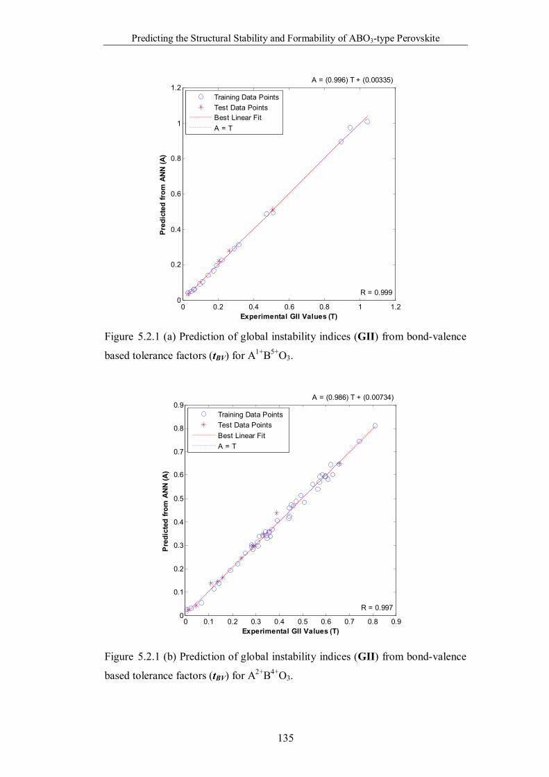
Predicting the Structural Stability and Formability of ABO3-type Perovskite
135
0 0.2 0.4 0.6 0.8 1 1.20
0.2
0.4
0.6
0.8
1
1.2
Experimental GII Values (T)
Pred
icte
d fr
om A
NN
(A)
A = (0.996) T + (0.00335)
R = 0.999
Training Data PointsTest Data PointsBest Linear FitA = T
Figure 5.2.1 (a) Prediction of global instability indices (GII) from bond-valence
based tolerance factors (tBV) for A1+B5+O3.
0 0.1 0.2 0.3 0.4 0.5 0.6 0.7 0.8 0.90
0.1
0.2
0.3
0.4
0.5
0.6
0.7
0.8
0.9
Experimental GII Values (T)
Pre
dict
ed fr
om A
NN
(A)
A = (0.986) T + (0.00734)
R = 0.997
Training Data PointsTest Data PointsBest Linear FitA = T
Figure 5.2.1 (b) Prediction of global instability indices (GII) from bond-valence
based tolerance factors (tBV) for A2+B4+O3.
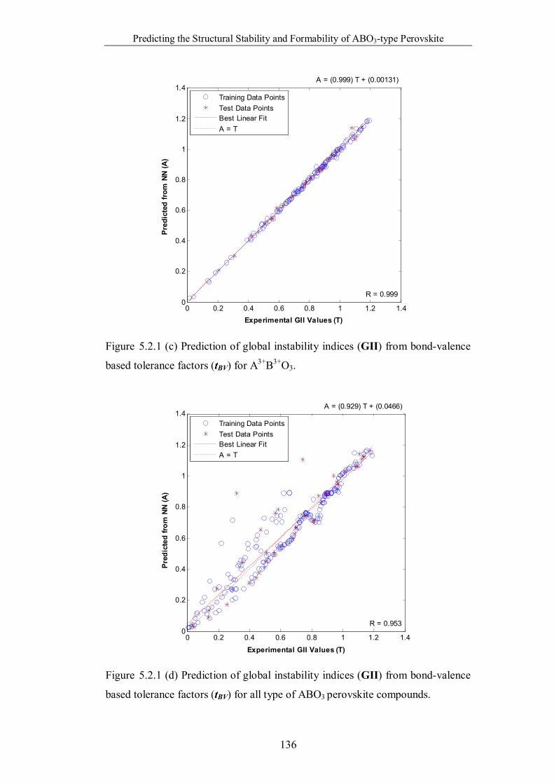
Predicting the Structural Stability and Formability of ABO3-type Perovskite
136
0 0.2 0.4 0.6 0.8 1 1.2 1.40
0.2
0.4
0.6
0.8
1
1.2
1.4
Experimental GII Values (T)
Pred
icte
d fr
om N
N (A
)
A = (0.999) T + (0.00131)
R = 0.999
Training Data PointsTest Data PointsBest Linear FitA = T
Figure 5.2.1 (c) Prediction of global instability indices (GII) from bond-valence
based tolerance factors (tBV) for A3+B3+O3.
0 0.2 0.4 0.6 0.8 1 1.2 1.40
0.2
0.4
0.6
0.8
1
1.2
1.4
Experimental GII Values (T)
Pred
icte
d fro
m N
N (A
)
A = (0.929) T + (0.0466)
R = 0.953
Training Data PointsTest Data PointsBest Linear FitA = T
Figure 5.2.1 (d) Prediction of global instability indices (GII) from bond-valence
based tolerance factors (tBV) for all type of ABO3 perovskite compounds.
Predicting the Structural Stability and Formability of ABO3-type Perovskite
137
Now the correlations between the tolerance factor and the overall structural
stability are explained. The overall structural stability, referred to as the global
instability index (GII), is determined by comparing the calculated atomic bond-
valence Vi(calc.) and formal valence Vi(OX), as used by Zhang et al. (2007),
2/1
1
2 /
NdGIIN
ii Equation 5.2.1
where N is the number of atoms in the asymmetric unit, and
)()( calciOXii VVd , j
ijcalci sV )( Equation 5.2.2
and
BdR
s ijijij exp Equation 5.2.3
where dij is the cation-anion bond distance; Rij is empirically determined for each
cation-anion pair based on a large number of well-determined bond distances for
the cation-anion pair in question, and has been tabulated; and B is an empirically
determined universal constant with a value of 0.37.
The bond-valence based tolerance factor, tBV, shown in Equation 5.2.4, is
calculated like the tolerance factor ()(2 OB
OA
rrrr
), but substituting rA+rO and
rB+rO with bond distances A-O (dAO) and B-O (dBO) calculated from the bond-
valence model.
BO
AO
dd2
BVt Equation 5.2.4
From the analysis above, it can be found that both the global instability index
(GII) and bond-valence tolerance factor (tBV) are calculated fundamentally from
dij and other parameters, and so there is a common response, as indicated in
Figure 1.5.1 (b), between GII and tBV. This can explain the results for each ABO3
type (A1+B5+O3, A2+B4+O3, A3+B3+O3) shown in Figure 5.2.1 (a)-(c); however, for
the whole range of ABO3-type perovskites, the correlation is rather poor, which
indicates that there is no unified relationship between tBV and GII for all the
types of ABO3 perovskite. However, if each GII value in Figure 1.8.1 were
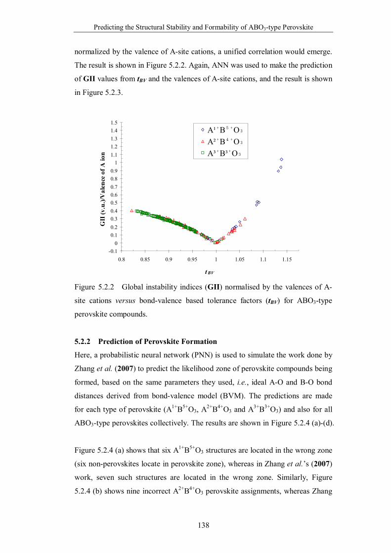
Predicting the Structural Stability and Formability of ABO3-type Perovskite
138
normalized by the valence of A-site cations, a unified correlation would emerge.
The result is shown in Figure 5.2.2. Again, ANN was used to make the prediction
of GII values from tBV and the valences of A-site cations, and the result is shown
in Figure 5.2.3.
-0.10
0.10.20.30.40.50.60.70.80.9
11.11.21.31.41.5
0.8 0.85 0.9 0.95 1 1.05 1.1 1.15
tBV
GII
(v.u
.)/V
alen
ce o
f A io
n
A¹⁺B⁵⁺O₃
A²⁺B⁴⁺O₃
A³⁺B³⁺O₃
Figure 5.2.2 Global instability indices (GII) normalised by the valences of A-
site cations versus bond-valence based tolerance factors (tBV) for ABO3-type
perovskite compounds.
5.2.2 Prediction of Perovskite Formation
Here, a probabilistic neural network (PNN) is used to simulate the work done by
Zhang et al. (2007) to predict the likelihood zone of perovskite compounds being
formed, based on the same parameters they used, i.e., ideal A-O and B-O bond
distances derived from bond-valence model (BVM). The predictions are made
for each type of perovskite (A1+B5+O3, A2+B4+O3 and A3+B3+O3) and also for all
ABO3-type perovskites collectively. The results are shown in Figure 5.2.4 (a)-(d).
Figure 5.2.4 (a) shows that six A1+B5+O3 structures are located in the wrong zone
(six non-perovskites locate in perovskite zone), whereas in Zhang et al.’s (2007)
work, seven such structures are located in the wrong zone. Similarly, Figure
5.2.4 (b) shows nine incorrect A2+B4+O3 perovskite assignments, whereas Zhang
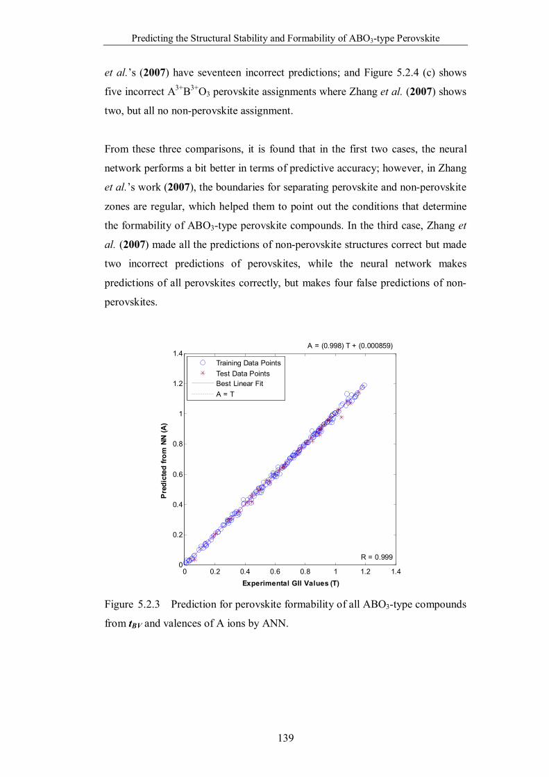
Predicting the Structural Stability and Formability of ABO3-type Perovskite
139
et al.’s (2007) have seventeen incorrect predictions; and Figure 5.2.4 (c) shows
five incorrect A3+B3+O3 perovskite assignments where Zhang et al. (2007) shows
two, but all no non-perovskite assignment.
From these three comparisons, it is found that in the first two cases, the neural
network performs a bit better in terms of predictive accuracy; however, in Zhang
et al.’s work (2007), the boundaries for separating perovskite and non-perovskite
zones are regular, which helped them to point out the conditions that determine
the formability of ABO3-type perovskite compounds. In the third case, Zhang et
al. (2007) made all the predictions of non-perovskite structures correct but made
two incorrect predictions of perovskites, while the neural network makes
predictions of all perovskites correctly, but makes four false predictions of non-
perovskites.
0 0.2 0.4 0.6 0.8 1 1.2 1.40
0.2
0.4
0.6
0.8
1
1.2
1.4
Experimental GII Values (T)
Pre
dict
ed fr
om N
N (A
)
A = (0.998) T + (0.000859)
R = 0.999
Training Data PointsTest Data PointsBest Linear FitA = T
Figure 5.2.3 Prediction for perovskite formability of all ABO3-type compounds
from tBV and valences of A ions by ANN.
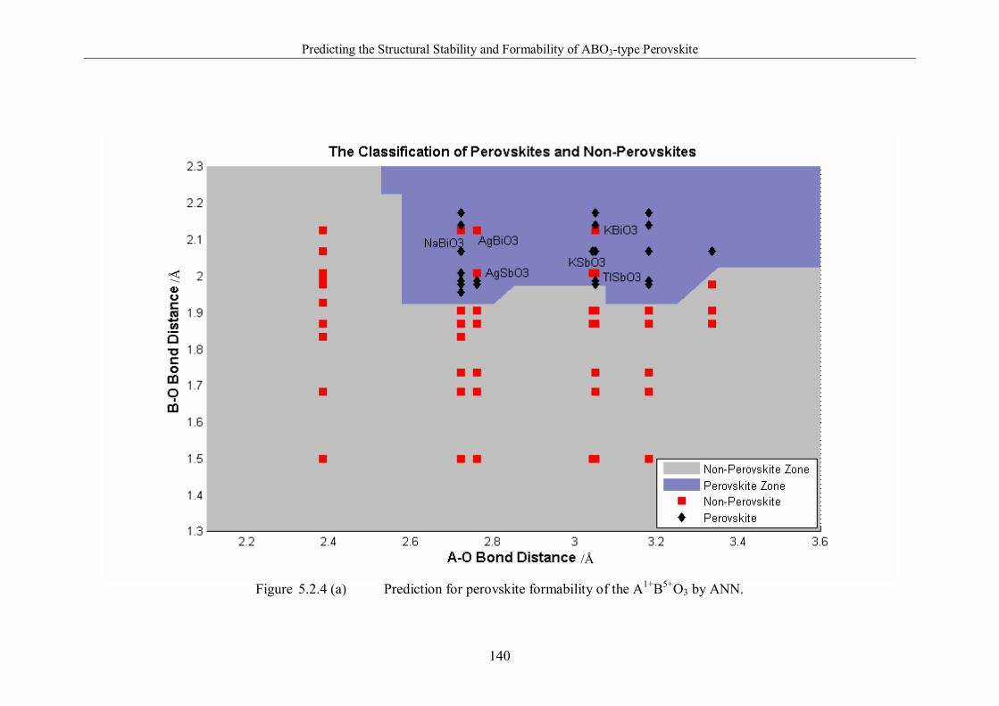
Predicting the Structural Stability and Formability of ABO3-type Perovskite
140
Figure 5.2.4 (a) Prediction for perovskite formability of the A1+B5+O3 by ANN.
/Å
/Å
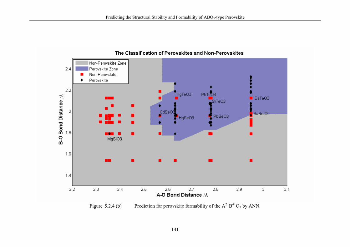
Predicting the Structural Stability and Formability of ABO3-type Perovskite
141
Figure 5.2.4 (b) Prediction for perovskite formability of the A2+B4+O3 by ANN.
/Å
/Å
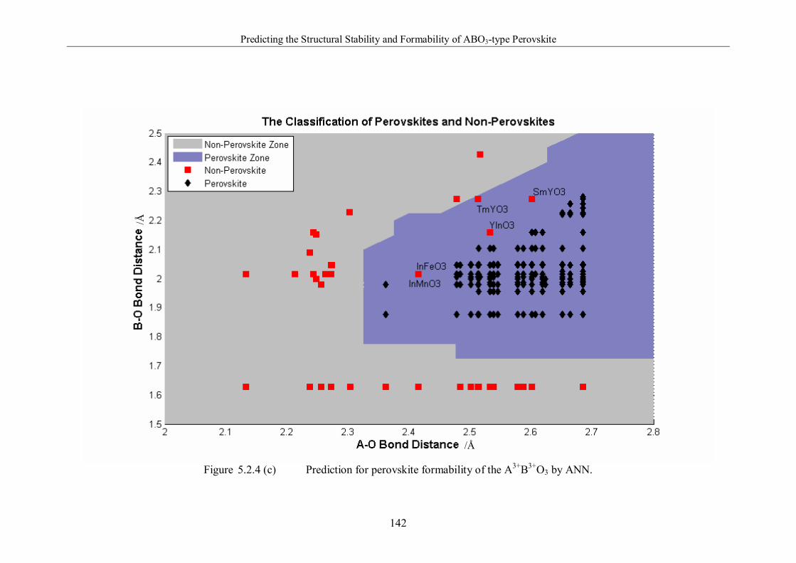
Predicting the Structural Stability and Formability of ABO3-type Perovskite
142
Figure 5.2.4 (c) Prediction for perovskite formability of the A3+B3+O3 by ANN.
/Å
/Å
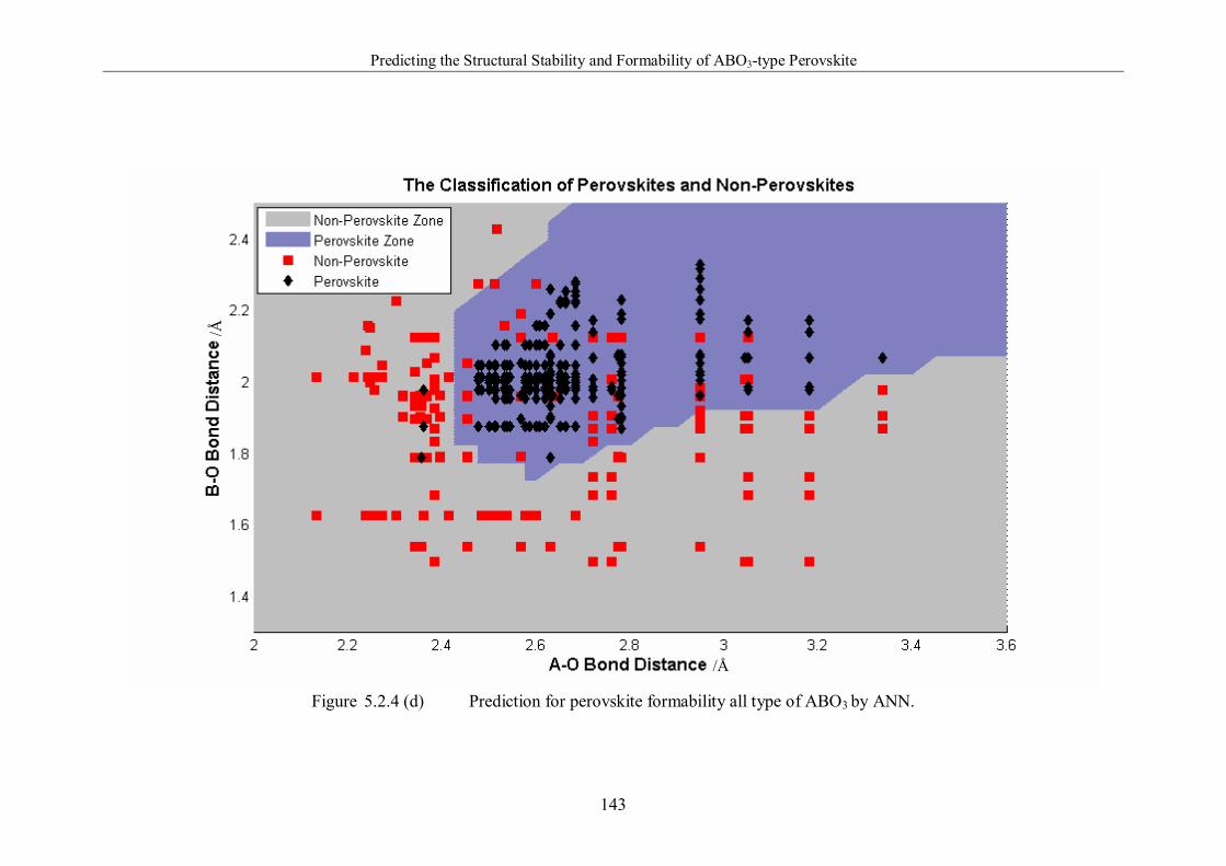
Predicting the Structural Stability and Formability of ABO3-type Perovskite
143
Figure 5.2.4 (d) Prediction for perovskite formability all type of ABO3 by ANN.
/Å
/Å
Exploring Unknown Cross-Properties Multiple Correlations using ANNs
144
6.0 Exploring unknown Cross-Properties Multiple
Correlations using ANNs 6.1 Specific Experimental Details
6.1.1 Data Collection
Whole datasets of physical properties of solid elements were collected from
handbooks, including Chemistry Data Handbook (CDH) (Start and Wallace,
1982), The Lange’s Handbook of Chemistry (LHC) (Speight, 2005), The
Elements (ELE) (Emsley, 1998), Table of Physical and Chemical Constants
(TPC) (Kaye and Laby, 1995) and CRC Handbook of Chemistry and Physics
(CRC) (David, 2000). The properties were collected for the same pressure (0.1
MPa), over a small temperature range (293~298 K) and in the solid state. The
sixteen properties collected were i) normal melting point, ii) normal boiling point,
iii) heat of fusion under normal melting point, iv) heat of vaporization under
normal boiling point, v) molar heat capacity, vi) specific heat capacity, vii)
thermal conductivity, viii) electrical conductivity, ix) photoelectric work function,
x) linear thermal expansion coefficient, xi) atomic weight, xii) density, xiii)
electronegativity (Pauling), xiv) first ionization potential, xv) polarizability and
xvi) atomic volume. The minor exceptions are mentioned in Tables A1 to A16
(Appendix 3). The elements for which data was collected satisfied two criteria: 1)
they are in solid state under 293~298 K and 0.1 MPa pressure; 2) they have a full
record of all sixteen properties from above five handbooks. The reason for those
criteria is: phase present, temperature and pressure are factors that would affect
some kinds of properties. However, introducing these three parameters would
weaken the generality of correlation between different properties due to the
common response of composition, structure and bonding. In total, 75 elements
are included.
From section 4, it has been found that there are always incorrect data in
handbooks. As a result, it is necessary to have an idea about the uncertainty of
the correctness for the data that is used and hence the uncertainty in the
correlation explored from using these data.
Exploring Unknown Cross-Properties Multiple Correlations using ANNs
145
The details of the data recorded from five different handbooks are listed in
Tables A1-A16 and are sorted with ascending levels of variability of property P;
(Pmax-Pmin)/Pmin. The data used for exploring property correlations are marked in
bold and were converted to SI units before being input. Most of the elements
have consistent values across the five handbooks and these values can be treated
as reliable. Data clustered in a narrow range can be treated as correct since they
are obtained from different sources. Identical data could have been copied.
Outliers are treated as incorrect due to incorrect unit conversions, decimal point
misplacements, different reference conditions or other reasons. Median values of
each property from five different recordings were treated as correct. The neural
network method developed in section 4 can be used to identify errors and select
correct values.
6.1.2 Pre-treatment of the Data
It is well known that the materials properties vary over considerable ranges and
are generally logarithmically distributed (Ashby, 1998; Bassetti et al., 1998;
Ashby et al., 2007). Sha (2008) noted that the network can be misled by a few
data far away from the average when training neural networks with skewed data
because, unlike linear regression, neural network training does not have a
definitive starting formula. For the neural network, logarithmic pre-treatment for
properties that are logarithmically distributed is needed.
The pre-treatment of the data was as follows. Electrical resistivity was converted
to electrical conductivity. From observation of these figures, it can be found that
the distribution of 1) atomic volume, 2) polarizability, 3) linear thermal
expansion coefficient, 4) electrical conductivity, 5) thermal conductivity, 6)
specific heat capacity and 7) heat of fusion are skewed. So these data need
logarithmic pre-treatment. However, from the data listed in Table A11 and
shown in Figure A1 (xi) (Appendix 4), the electrical conductivity disperses over
such a large range that taking logarithmic pre-treatment cannot normalize the
distribution. Further, some data can be interpreted as sensitive to impurities (e.g.
Si, Ge), and this introduces uncertainties for extracting a general correlation
between properties. As a result, electrical conductivity was not introduced for
exploration of property relationships. Figures A2 (i)-(vi) show the distribution of
Exploring Unknown Cross-Properties Multiple Correlations using ANNs
146
these six properties after taking logarithms. From Figure A2 (i)-(vi), the values
for atomic volume, polarizability, linear thermal expansion coefficient and heat
of fusion become uniformly distributed; while for thermal conductivity and
specific heat capacity, the distributions are enhanced.
As a result, the whole group of property values are 1) melting point (original
value), 2) boiling point (original value), 3) atomic volume (logarithmic value), 4)
polarizability (logarithmic value), 5) first ionization potential (original value), 6)
electronegativity (original value), 7) density (original value), 8) atomic weight
(original value), 9) linear thermal expansion coefficient (logarithmic value), 10)
photonic work function (original value), 11) thermal conductivity (logarithmic
value), 12) specific heat capacity (logarithmic value), 13) molar heat capacity
(original value), 14) heat of vaporization (original value), 15) heat of fusion
(logarithmic value). All or part of these property values constitute inputs for the
neural network. Each of them in turn is also used as an output. When property
values were used for output, the original values were adopted, because the neural
network training is based on minimization of the difference between predicted
values and experimental values. And small differences in logarithmic values
correspond to large differences in original values.
6.1.3 Determination of Input and Output Parameters
Of all sixteen properties, one is taken as the property to be predicted (as an
output of the neural network) in turn, and all other properties left constitute a
whole set. Within the whole set, different numbers of properties with different
combinations were chosen to form property groups used for predicting the named
property (as input parameters of the neural networks). This process was repeated
by taking each of sixteen properties one by one as a property to be predicted.
Finally, when some properties values can be reasonably predicted from groups of
other properties, then we can say that all of these properties are correlated.
When considering how to find the closest and highest performance for both
training and testing sets, a distribution was selected on the basis of 2testing
2training , where = )R(M 11 , and the smallest value of was chosen.
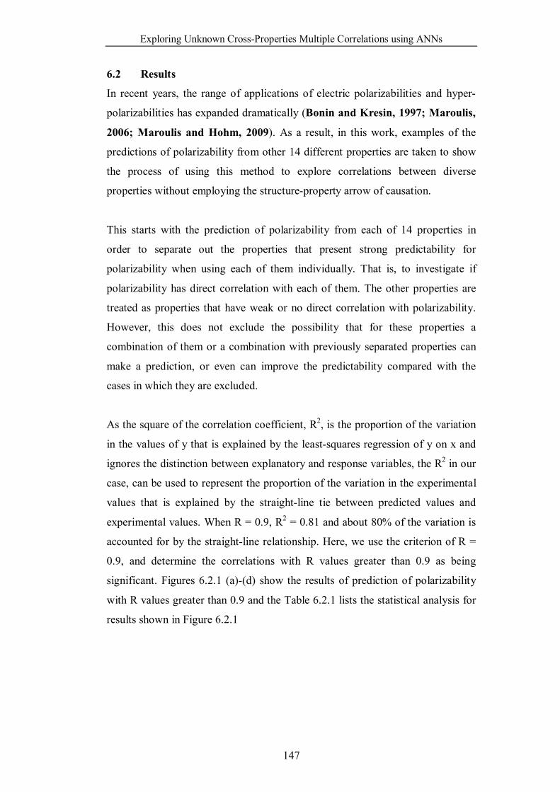
Exploring Unknown Cross-Properties Multiple Correlations using ANNs
147
6.2 Results
In recent years, the range of applications of electric polarizabilities and hyper-
polarizabilities has expanded dramatically (Bonin and Kresin, 1997; Maroulis,
2006; Maroulis and Hohm, 2009). As a result, in this work, examples of the
predictions of polarizability from other 14 different properties are taken to show
the process of using this method to explore correlations between diverse
properties without employing the structure-property arrow of causation.
This starts with the prediction of polarizability from each of 14 properties in
order to separate out the properties that present strong predictability for
polarizability when using each of them individually. That is, to investigate if
polarizability has direct correlation with each of them. The other properties are
treated as properties that have weak or no direct correlation with polarizability.
However, this does not exclude the possibility that for these properties a
combination of them or a combination with previously separated properties can
make a prediction, or even can improve the predictability compared with the
cases in which they are excluded.
As the square of the correlation coefficient, R2, is the proportion of the variation
in the values of y that is explained by the least-squares regression of y on x and
ignores the distinction between explanatory and response variables, the R2 in our
case, can be used to represent the proportion of the variation in the experimental
values that is explained by the straight-line tie between predicted values and
experimental values. When R = 0.9, R2 = 0.81 and about 80% of the variation is
accounted for by the straight-line relationship. Here, we use the criterion of R =
0.9, and determine the correlations with R values greater than 0.9 as being
significant. Figures 6.2.1 (a)-(d) show the results of prediction of polarizability
with R values greater than 0.9 and the Table 6.2.1 lists the statistical analysis for
results shown in Figure 6.2.1
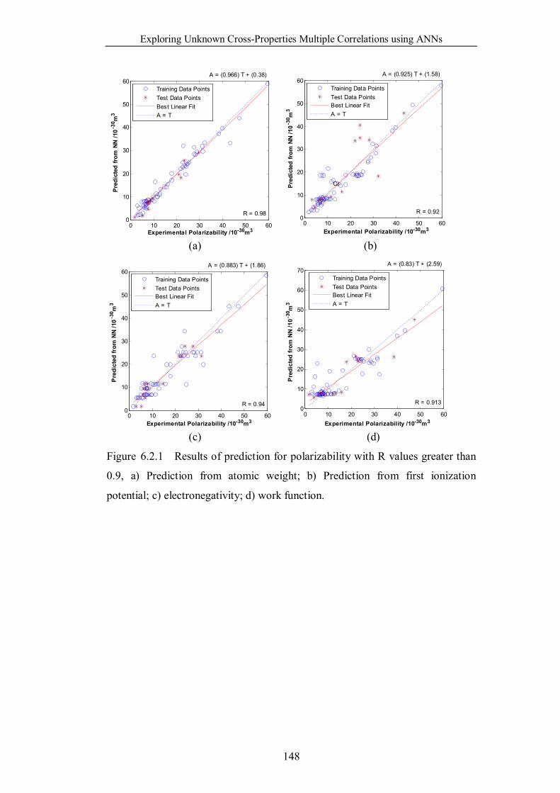
Exploring Unknown Cross-Properties Multiple Correlations using ANNs
148
0 10 20 30 40 50 600
10
20
30
40
50
60
Experimental Polarizability /10-30m3
Pred
icte
d fro
m N
N /1
0-30 m
3
A = (0.966) T + (0.38)
R = 0.98
Training Data PointsTest Data PointsBest Linear FitA = T
0 10 20 30 40 50 60
0
10
20
30
40
50
60
Experimental Polarizability /10-30m3
Pred
icte
d fro
m N
N /1
0-30 m
3
A = (0.925) T + (1.58)
R = 0.92
Cr
Training Data PointsTest Data PointsBest Linear FitA = T
(a) (b)
0 10 20 30 40 50 600
10
20
30
40
50
60
Experimental Polarizability /10-30m3
Pre
dict
ed fr
om N
N /1
0-3
0 m3
A = (0.883) T + (1.86)
R = 0.94
Training Data PointsTest Data PointsBest Linear FitA = T
0 10 20 30 40 50 60
0
10
20
30
40
50
60
70
Experimental Polarizability /10-30m3
Pre
dict
ed fr
om N
N /1
0-30 m
3
A = (0.83) T + (2.59)
R = 0.913
Training Data PointsTest Data PointsBest Linear FitA = T
(c) (d)
Figure 6.2.1 Results of prediction for polarizability with R values greater than
0.9, a) Prediction from atomic weight; b) Prediction from first ionization
potential; c) electronegativity; d) work function.
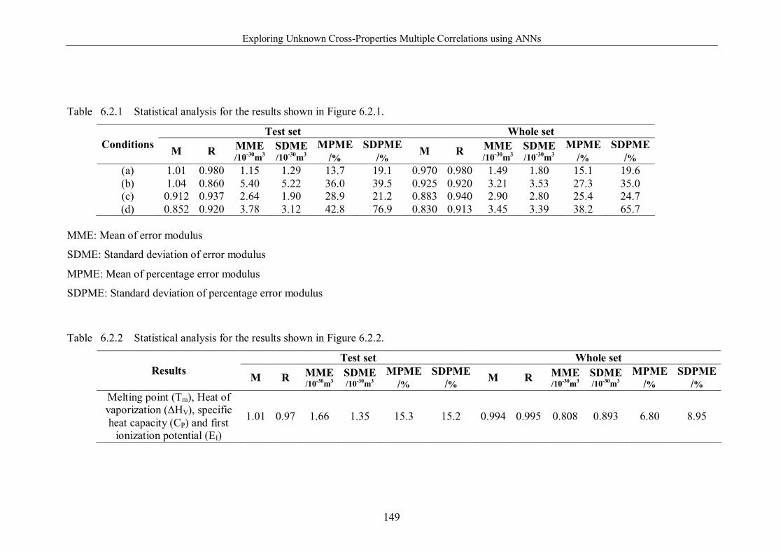
Exploring Unknown Cross-Properties Multiple Correlations using ANNs
149
Table 6.2.1 Statistical analysis for the results shown in Figure 6.2.1.
Test set Whole set Conditions M R MME
/10-30m3 SDME /10-30m3
MPME /%
SDPME /% M R MME
/10-30m3 SDME /10-30m3
MPME /%
SDPME /%
(a) 1.01 0.980 1.15 1.29 13.7 19.1 0.970 0.980 1.49 1.80 15.1 19.6 (b) 1.04 0.860 5.40 5.22 36.0 39.5 0.925 0.920 3.21 3.53 27.3 35.0 (c) 0.912 0.937 2.64 1.90 28.9 21.2 0.883 0.940 2.90 2.80 25.4 24.7 (d) 0.852 0.920 3.78 3.12 42.8 76.9 0.830 0.913 3.45 3.39 38.2 65.7
MME: Mean of error modulus
SDME: Standard deviation of error modulus
MPME: Mean of percentage error modulus
SDPME: Standard deviation of percentage error modulus
Table 6.2.2 Statistical analysis for the results shown in Figure 6.2.2.
Test set Whole set Results M R MME
/10-30m3 SDME /10-30m3
MPME /%
SDPME /% M R MME
/10-30m3 SDME /10-30m3
MPME /%
SDPME /%
Melting point (Tm), Heat of vaporization (ΔHV), specific heat capacity (CP) and first
ionization potential (EI)
1.01 0.97 1.66 1.35 15.3 15.2 0.994 0.995 0.808 0.893 6.80 8.95
Exploring Unknown Cross-Properties Multiple Correlations using ANNs
150
Thus we have located four properties that have relatively strong correlations with
polarizability and separated the other ten properties that have relative weak or
even no correlations with polarizability. In the next step, based on these four
properties, systematically to introduce other properties to see if continuous
improvements in the prediction results, and thus to find the effect of each
property on the prediction. However, the properties are obtained from different
levels of structure, or even combinations of different levels of structure, and so
these properties can be treated as confounding effects of different levels of
structure, as shown in Figure 1.5.1(c). It needs to be clarified that the correlations
between structures and properties are direct cause-effect, while those between
different levels of structure and properties may be confounding. As a result, the
correlations between the properties that are used for making prediction may also
be confounding. As mentioned in section 1.5.2, since the effects of properties are
confounded together, the influence of one property cannot be distinguished from
the influence of other properties; also, it cannot be said how strong the effect of
one property on polarizability is. This leads to some properties, which cannot
make a prediction alone, having an effect or even a strong effect on the
prediction when combined with other properties.
So, in this step, it focus on the results that show a high degree of correlation
between polarizability and different combinations of other properties, and then
from these results, try to find the underlying physical principles and the reasons
why different combinations of properties can have similar prediction
performance. The criterion used here is R2 = 99%, which corresponding to R =
0.995 and the slope M equal to or greater than 0.99. In total, there are 665
combinations of different numbers of different kinds of properties. These
different combinations are treated as having the same capability for prediction of
polarizability. Due to the confounding effect mentioned before, it is still difficult
to employ a systematic method. In this work, it started from the analysis of the
results for the prediction using a combination of the minimum number of
properties, namely the prediction of polarizability from melting point, heat of
vaporization, specific heat capacity and first ionization potential. The results are
shown in Figure 6.2.2, and the statistical analysis for these results are shown in
Table 6.2.2.
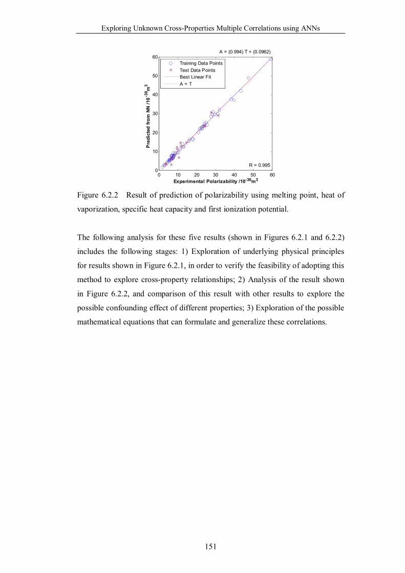
Exploring Unknown Cross-Properties Multiple Correlations using ANNs
151
0 10 20 30 40 50 600
10
20
30
40
50
60
Experimental Polarizability /10-30m3
Pre
dict
ed fr
om N
N /1
0-30 m
3
A = (0.994) T + (0.0962)
R = 0.995
Training Data PointsTest Data PointsBest Linear FitA = T
Figure 6.2.2 Result of prediction of polarizability using melting point, heat of
vaporization, specific heat capacity and first ionization potential.
The following analysis for these five results (shown in Figures 6.2.1 and 6.2.2)
includes the following stages: 1) Exploration of underlying physical principles
for results shown in Figure 6.2.1, in order to verify the feasibility of adopting this
method to explore cross-property relationships; 2) Analysis of the result shown
in Figure 6.2.2, and comparison of this result with other results to explore the
possible confounding effect of different properties; 3) Exploration of the possible
mathematical equations that can formulate and generalize these correlations.
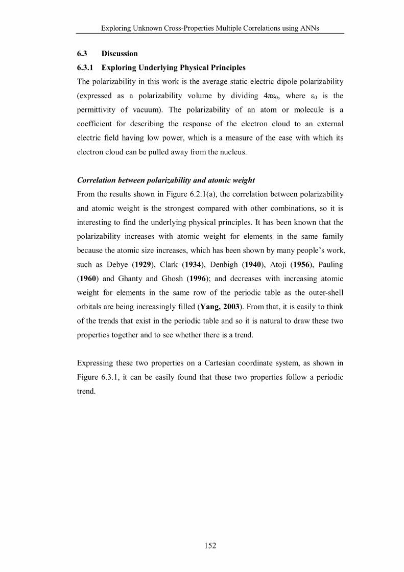
Exploring Unknown Cross-Properties Multiple Correlations using ANNs
152
6.3 Discussion
6.3.1 Exploring Underlying Physical Principles
The polarizability in this work is the average static electric dipole polarizability
(expressed as a polarizability volume by dividing 4πε0, where ε0 is the
permittivity of vacuum). The polarizability of an atom or molecule is a
coefficient for describing the response of the electron cloud to an external
electric field having low power, which is a measure of the ease with which its
electron cloud can be pulled away from the nucleus.
Correlation between polarizability and atomic weight
From the results shown in Figure 6.2.1(a), the correlation between polarizability
and atomic weight is the strongest compared with other combinations, so it is
interesting to find the underlying physical principles. It has been known that the
polarizability increases with atomic weight for elements in the same family
because the atomic size increases, which has been shown by many people’s work,
such as Debye (1929), Clark (1934), Denbigh (1940), Atoji (1956), Pauling
(1960) and Ghanty and Ghosh (1996); and decreases with increasing atomic
weight for elements in the same row of the periodic table as the outer-shell
orbitals are being increasingly filled (Yang, 2003). From that, it is easily to think
of the trends that exist in the periodic table and so it is natural to draw these two
properties together and to see whether there is a trend.
Expressing these two properties on a Cartesian coordinate system, as shown in
Figure 6.3.1, it can be easily found that these two properties follow a periodic
trend.
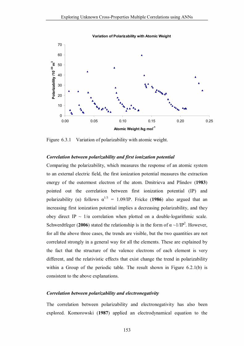
Exploring Unknown Cross-Properties Multiple Correlations using ANNs
153
Variation of Polarizability with Atomic Weight
0
10
20
30
40
50
60
70
0.00 0.05 0.10 0.15 0.20 0.25
Atomic Weight /kg mol-1
Pola
rizab
ility
/10-3
0 m
3
Figure 6.3.1 Variation of polarizability with atomic weight.
Correlation between polarizability and first ionization potential
Comparing the polarizability, which measures the response of an atomic system
to an external electric field, the first ionization potential measures the extraction
energy of the outermost electron of the atom. Dmitrieva and Plindov (1983)
pointed out the correlation between first ionization potential (IP) and
polarizability (α) follows α1/3 = 1.09/IP. Fricke (1986) also argued that an
increasing first ionization potential implies a decreasing polarizability, and they
obey direct IP ~ 1/α correlation when plotted on a double-logarithmic scale.
Schwerdtfeger (2006) stated the relationship is in the form of α ~1/IP2. However,
for all the above three cases, the trends are visible, but the two quantities are not
correlated strongly in a general way for all the elements. These are explained by
the fact that the structure of the valence electrons of each element is very
different, and the relativistic effects that exist change the trend in polarizability
within a Group of the periodic table. The result shown in Figure 6.2.1(b) is
consistent to the above explanations.
Correlation between polarizability and electronegativity
The correlation between polarizability and electronegativity has also been
explored. Komorowski (1987) applied an electrodynamical equation to the
Exploring Unknown Cross-Properties Multiple Correlations using ANNs
154
chemical potential by analogy and got an inverse relationship between
polarizability and electronegativity; Van Genechten et al. (1987) applied the
electronegativity equalization method to calculate values of average
electronegativity and related these values to the polarizability: large
electronegativity is consistent with a low polarizability. However, in these two
works, the correlations are not explored in detail. Nagle (1990) employed the
concept of valence electron density (Gorbunov and Kaganyuk, 1986;
Gorbunov and Filippov, 1988), and got a function of the number of valence
electrons divided by polarizability, n/α. Then, the cube root of this ratio, (n/α)1/3,
can be used for calculating the electronegativity χ: χ = 1.66 (n/α)1/3 + 0.37 for s-
and p-block elements, and it also can be applied to d- and f-block elements if the
number of “valence” electrons for these elements can be determined from a
careful analysis of their atomic spectra. Further proofs can be derived from the
facts that there are correlations existing between atomic radii and polarizability,
and also between atomic radii and electronegativity, such as the work done by
Ghanty and Ghosh (1996). So, the polarizability and electronegativity can be
treated as common responses from atomic radii, as shown in Figure 1.5.1(b). The
discussion in the above cases describes the relationship between polarizability
and electronegativity from a physical perspective, and also states there is no
direct relationship between them. In order to make a comprehensive and general
prediction, other parameters must be introduced.
Correlation between polarizability and work function
The electron work function ø is a measure of the minimum energy required to
extract an electron from the surface of a solid, which was first pointed out by
Lester (1916). It can be measured from thermionic, photoelectric or contact
potential methods. Different methods are applied in different conditions. As
mentioned by Michaelson (1977), the thermionic method cannot give the
absolute value for polycrystalline or other patchy surfaces, while the
photoelectric method does not yield the true work function for semiconductors
because the emission contains contributions of both volume and surface origin.
The critical review of different measurement methods and the rationale for
selecting preferred values are discussed by Rivière (1969).
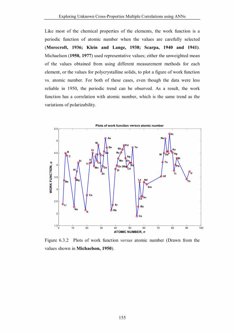
Exploring Unknown Cross-Properties Multiple Correlations using ANNs
155
Like most of the chemical properties of the elements, the work function is a
periodic function of atomic number when the values are carefully selected
(Morecroft, 1936; Klein and Lange, 1938; Scarpa, 1940 and 1941).
Michaelson (1950, 1977) used representative values; either the unweighted mean
of the values obtained from using different measurement methods for each
element, or the values for polycrystalline solids, to plot a figure of work function
vs. atomic number. For both of these cases, even though the data were less
reliable in 1950, the periodic trend can be observed. As a result, the work
function has a correlation with atomic number, which is the same trend as the
variations of polarizability.
0 10 20 30 40 50 60 70 80 90 1001.5
2
2.5
3
3.5
4
4.5
5
5.5
Li
Be
BC
Na
Mg
Al
Si
K
Ca
TiV
Cr
Mn
Fe
Co
Ni
Cu
Zn
Ga
Ge
As
Se
Rb
Sr
ZrCb (Nb)
Mo
RuRh
Pd
Ag
Cd
Sn
Sb
Te
Cs
Ba
La
Ce Pr
Nd
Sm
Hf
Ta
W
Re
OsIr
Pt
AuHg
Tl
Pb
Bi
Th
U
ATOMIC NUMBER, n
WO
RK
FU
NC
TIO
N,
Plots of work function versus atomic number
Figure 6.3.2 Plots of work function versus atomic number (Drawn from the
values shown in Michaelson, 1950).
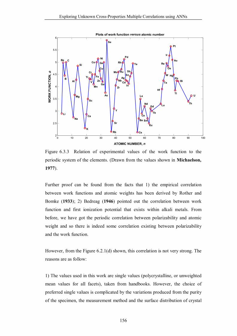
Exploring Unknown Cross-Properties Multiple Correlations using ANNs
156
0 10 20 30 40 50 60 70 80 90 1002
2.5
3
3.5
4
4.5
5
5.5
6
Li
Be
B
C
Na
Mg
Al
Si
K
Ca
Sc
Ti
V
Cr
Mn
Fe
CoNi
Cu
ZnGa
Ge
As
Se
Rb
Sr
Y
Zr
Nb
Mo Ru
Rh
Pd
Ag
CdIn
SnSb
Te
Cs
Ba
La
Ce
Nd
Sm
Eu
Gd
Tb
Lu
Hf
Ta
W
Re
Os
Ir
Pt
Au
Hg
Tl
PbBi
Th
U
Plots of work function versus atomic number
ATOMIC NUMBER, n
WO
RK
FU
NC
TIO
N,
Figure 6.3.3 Relation of experimental values of the work function to the
periodic system of the elements. (Drawn from the values shown in Michaelson,
1977).
Further proof can be found from the facts that 1) the empirical correlation
between work functions and atomic weights has been derived by Rother and
Bomke (1933); 2) Bedreag (1946) pointed out the correlation between work
function and first ionization potential that exists within alkali metals. From
before, we have got the periodic correlation between polarizability and atomic
weight and so there is indeed some correlation existing between polarizability
and the work function.
However, from the Figure 6.2.1(d) shown, this correlation is not very strong. The
reasons are as follow:
1) The values used in this work are single values (polycrystalline, or unweighted
mean values for all facets), taken from handbooks. However, the choice of
preferred single values is complicated by the variations produced from the purity
of the specimen, the measurement method and the surface distribution of crystal
Exploring Unknown Cross-Properties Multiple Correlations using ANNs
157
facets (Michaelson, 1977). Firstly, the measurements of work function are
extremely sensitive to the presence of surface impurities, such as oxides and
gases (Michaelson, 1950). When the measurement is not carried out under
ultrahigh vacua, the result is affected by trace impurities (Michaelson, 1977). An
example is the value for Be. It has been accepted that the value is 5 eV, as
employed in this work, as determined first by Dixon and Lott (1969) and
confirmed later by Gustafsson et al. (1974). However, the previously accepted
value is about 3.9 eV, as recorded in Table of Physical and Chemical Constants
(as shown in Table A10), which is due to mercury vapour contamination. Further,
the anisotropy (Martin, 1939; Smoluchowski, 1941), allotropy (Goetz, 1929;
Wahlin, 1942) and temperature dependence (Potter, 1940; Seely, 1941; Smith,
1949; Markham and Miller, 1949) complicate the values of work functions,
although the difference is not great. The data recorded in handbooks have these
uncertainties.
2) For semiconductor elements, variations, although not great, exist among the
values obtained from different methods of measurement (Condon, 1938; Apker
et al., 1948). Also, for the data for As (Raisin and Pinchaux, 1975), Te
(Williams and Polanco, 1974) and Se (Williams and Polanco, 1974), which
belong to semiconductors, are derived from photoelectric methods. It is stated
before that the photoelectric method cannot yield the true work function for
semiconductors. Actually, these values cannot be confirmed by measurements
made with ultrahigh vacuum techniques. So, as suggested by Michaelson (1977),
these values are only to be treated as possibly valid but of unknown reliability,
and only can be accepted simply as being the best available and not necessarily
as absolute physical quantities.
3) The periodic trend found by Michaelson (1950, 1977), as shown in Figures
6.3.2 and 6.3.3, is obvious, but not rigorous. As mentioned by him, in each
period, the work function value tends to rise with increasing atomic number, as
electron shells and subshells gradually become filled; however, the relation
becomes complex in the intervals occupied by the transition metals.
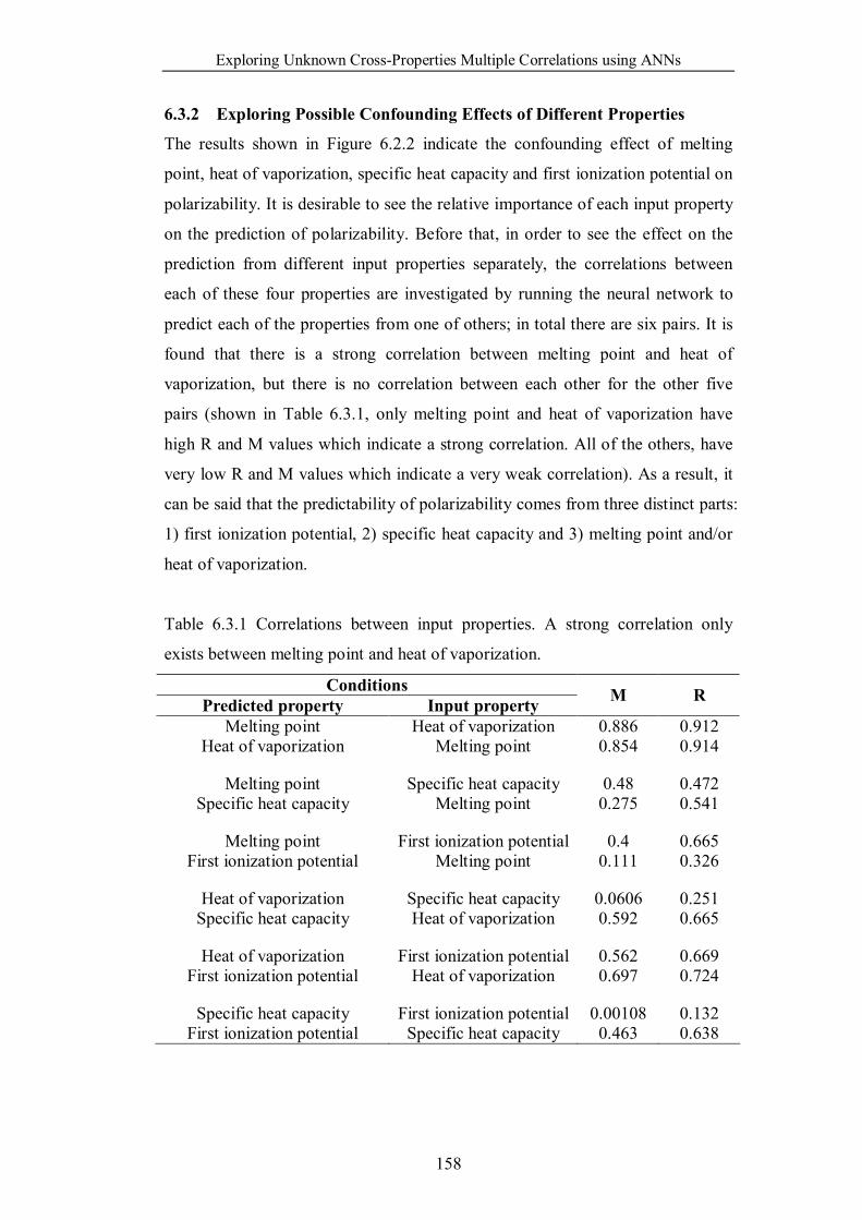
Exploring Unknown Cross-Properties Multiple Correlations using ANNs
158
6.3.2 Exploring Possible Confounding Effects of Different Properties
The results shown in Figure 6.2.2 indicate the confounding effect of melting
point, heat of vaporization, specific heat capacity and first ionization potential on
polarizability. It is desirable to see the relative importance of each input property
on the prediction of polarizability. Before that, in order to see the effect on the
prediction from different input properties separately, the correlations between
each of these four properties are investigated by running the neural network to
predict each of the properties from one of others; in total there are six pairs. It is
found that there is a strong correlation between melting point and heat of
vaporization, but there is no correlation between each other for the other five
pairs (shown in Table 6.3.1, only melting point and heat of vaporization have
high R and M values which indicate a strong correlation. All of the others, have
very low R and M values which indicate a very weak correlation). As a result, it
can be said that the predictability of polarizability comes from three distinct parts:
1) first ionization potential, 2) specific heat capacity and 3) melting point and/or
heat of vaporization.
Table 6.3.1 Correlations between input properties. A strong correlation only
exists between melting point and heat of vaporization.
Conditions Predicted property Input property M R
Melting point Heat of vaporization 0.886 0.912 Heat of vaporization Melting point 0.854 0.914
Melting point Specific heat capacity 0.48 0.472 Specific heat capacity Melting point 0.275 0.541
Melting point First ionization potential 0.4 0.665 First ionization potential Melting point 0.111 0.326
Heat of vaporization Specific heat capacity 0.0606 0.251 Specific heat capacity Heat of vaporization 0.592 0.665
Heat of vaporization First ionization potential 0.562 0.669 First ionization potential Heat of vaporization 0.697 0.724
Specific heat capacity First ionization potential 0.00108 0.132 First ionization potential Specific heat capacity 0.463 0.638
Exploring Unknown Cross-Properties Multiple Correlations using ANNs
159
In the following stage, the relative importance of each property is explored.
Based on the result shown in Figure 6.2.2, the relative importance of each
property is compared by running the network with one input property omitted at
a time and the results are shown in Table 6.3.2. From observing all the
parameters for these four different cases, it can easily be found that the relative
importance of each property for the prediction of polarizability follows a
descending order: first ionization potential, melting point, heat of vaporization
and specific heat capacity. That is, the predictability of polarizability mostly
comes from the first ionization potential, then smaller parts from melting point
and heat of vaporization (also, melting point contributes more than heat of
vaporization), and the smallest part comes from specific heat capacity.
The strong correlation between polarizability and first ionization potential has
been discussed in the previous section. The correlations between polarizability
and the other three properties (i.e. melting point, heat of vaporization and
specific heat capacity) are compared in Table 6.3.3. From looking at these results,
it can easily be found that the correlation between polarizability and these three
properties are weak, following the order of degree of weakness: heat of
vaporization, melting point and specific heat capacity. From this, it can be seen
that although these properties have weak correlations with polarizability, the
predictability can be improved when confound with the other two properties;
notably, the melting point makes more contribution to the predictability of
polarizability than heat of vaporization, when confound with the other two
properties, although the predictability is weaker than heat of vaporization when
used alone.
In the next stage, pairs of parameters are selected to predict polarizability: (1)
melting point and heat of vaporization; (2) melting point and specific heat
capacity; (3) heat of vaporization and specific heat capacity; (4) specific heat
capacity and first ionization potential; (5) heat of vaporization and first ionization
potential and (6) melting point and first ionization potential. They are shown in
Table 6.3.4.
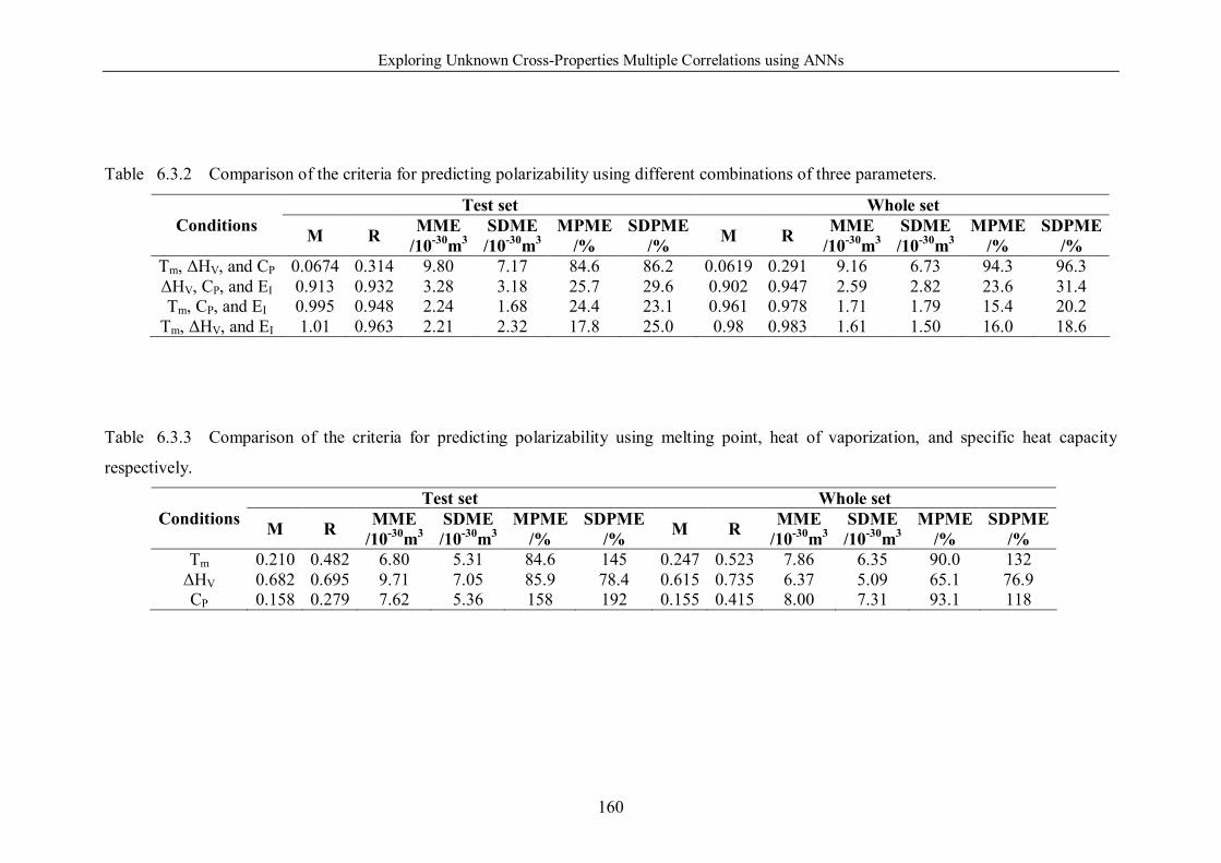
Exploring Unknown Cross-Properties Multiple Correlations using ANNs
160
Table 6.3.2 Comparison of the criteria for predicting polarizability using different combinations of three parameters.
Test set Whole set Conditions M R MME
/10-30m3 SDME /10-30m3
MPME /%
SDPME /% M R MME
/10-30m3 SDME /10-30m3
MPME /%
SDPME /%
Tm, ΔHV, and CP 0.0674 0.314 9.80 7.17 84.6 86.2 0.0619 0.291 9.16 6.73 94.3 96.3 ΔHV, CP, and EI 0.913 0.932 3.28 3.18 25.7 29.6 0.902 0.947 2.59 2.82 23.6 31.4 Tm, CP, and EI 0.995 0.948 2.24 1.68 24.4 23.1 0.961 0.978 1.71 1.79 15.4 20.2
Tm, ΔHV, and EI 1.01 0.963 2.21 2.32 17.8 25.0 0.98 0.983 1.61 1.50 16.0 18.6
Table 6.3.3 Comparison of the criteria for predicting polarizability using melting point, heat of vaporization, and specific heat capacity
respectively.
Test set Whole set Conditions M R MME
/10-30m3 SDME /10-30m3
MPME /%
SDPME /% M R MME
/10-30m3 SDME /10-30m3
MPME /%
SDPME /%
Tm 0.210 0.482 6.80 5.31 84.6 145 0.247 0.523 7.86 6.35 90.0 132 ΔHV 0.682 0.695 9.71 7.05 85.9 78.4 0.615 0.735 6.37 5.09 65.1 76.9 CP 0.158 0.279 7.62 5.36 158 192 0.155 0.415 8.00 7.31 93.1 118
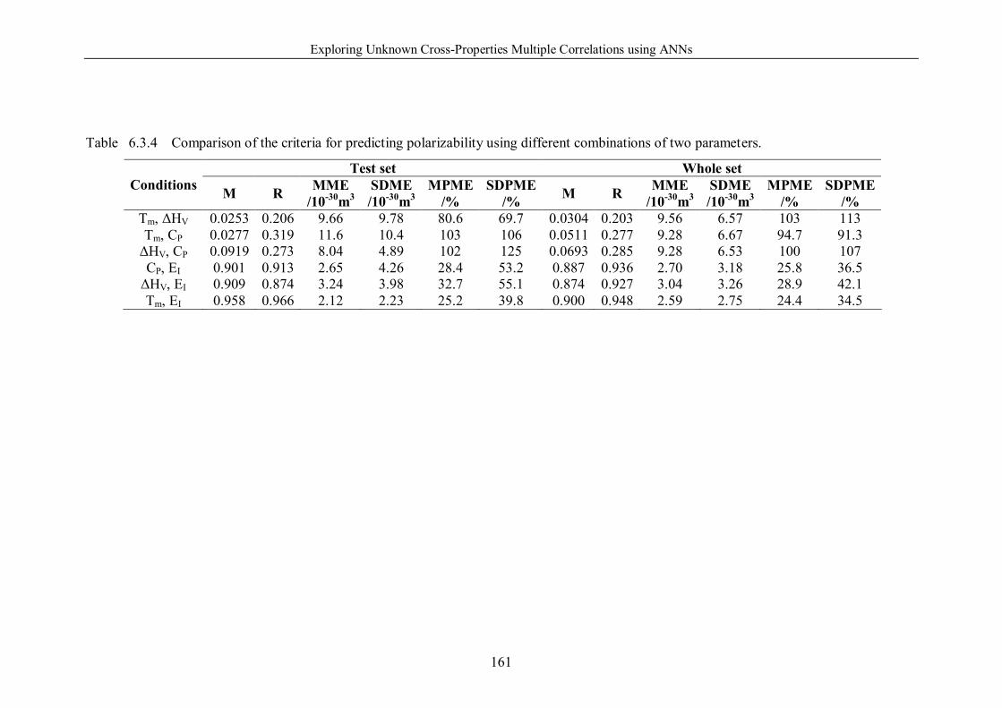
Exploring Unknown Cross-Properties Multiple Correlations using ANNs
161
Table 6.3.4 Comparison of the criteria for predicting polarizability using different combinations of two parameters.
Test set Whole set Conditions M R MME
/10-30m3 SDME /10-30m3
MPME /%
SDPME /% M R MME
/10-30m3 SDME /10-30m3
MPME /%
SDPME /%
Tm, ΔHV 0.0253 0.206 9.66 9.78 80.6 69.7 0.0304 0.203 9.56 6.57 103 113 Tm, CP 0.0277 0.319 11.6 10.4 103 106 0.0511 0.277 9.28 6.67 94.7 91.3
ΔHV, CP 0.0919 0.273 8.04 4.89 102 125 0.0693 0.285 9.28 6.53 100 107 CP, EI 0.901 0.913 2.65 4.26 28.4 53.2 0.887 0.936 2.70 3.18 25.8 36.5
ΔHV, EI 0.909 0.874 3.24 3.98 32.7 55.1 0.874 0.927 3.04 3.26 28.9 42.1 Tm, EI 0.958 0.966 2.12 2.23 25.2 39.8 0.900 0.948 2.59 2.75 24.4 34.5
Exploring Unknown Cross-Properties Multiple Correlations using ANNs
162
From observing these results, it can be found that the combination of melting
point and heat of vaporization has the weakest predictability. The reason is that,
as mention before, the predictability of polarizability comes from three parts and
due to the correlation that exists between melting point and heat of vaporization,
the effect of melting point and heat of vaporization can be treated as the same
one part and this single part cannot make the prediction better. Then from the
second and third row, the role of specific heat capacity is introduced, and the
performance is improved and from these two results, it is also found that when
confounded with specific heat capacity, the heat of vaporization has better
prediction performance than melting point, which is consistent with the trend
when using melting point or heat of vaporization alone. From looking at rows 4
to 6, the first ionization potential is introduced, which has a single correlation
with polarizability and the performance is improved further. Observing these
three rows confirms the ascending effect of specific heat capacity, heat of
vaporization and melting point on the prediction of polarizability when confound
with polarizability as discussed before.
From the discussions made above, it can be concluded that: within the group of
properties consisting of melting point, heat of vaporization, specific heat capacity
and first ionization potential, the first ionization potential plays the most
important part, the melting point and heat of vaporization play a similar role and
the second most important effect while the specific heat capacity plays the least
important part. For melting point and heat of vaporization, the heat of
vaporization has higher predictability for polarizability when testing each of
them alone, or confounding each with specific heat capacity. However, when
confound with first ionization potential, the melting point has a higher
performance. For all the inputs that do not adopt the property of first ionization
potential, the correlations with polarizability are very weak; however, when they
are confounded with first ionization potential, the performance is improved a lot
(from M=0.925, R=0.92 to M=0.994, R=0.995).
Exploring Unknown Cross-Properties Multiple Correlations using ANNs
163
6.3.3 Exploration of Possible Mathematical Equations that can Formulate
Correlations
To extend these ideas, it would be more interesting to find possible mathematical
functions that can describe the correlations found by the neural network.
Recently this has been demonstrated by Schmidt and Lipson (2009), who used
genetic programming to extract Hamiltonians and other laws by automatically
searching motion-tracking data captured from chaotic double-pendula. So it will
be possible to find mathematical equations from these correlations in the future.
However, in the method proposed by Schmidt and Lipson (2009), researchers
still need to identify mathematical building blocks such as algebraic operators,
analytical functions, etc. So, it is reasonable to speculate some building blocks by
visualizing the functional relationship which is captured by the neural network,
in order to see the variance of polarizability in terms of the input properties.
However, for the result shown in Figure 6.2.2, the neural network captured the
correlation between polarizability and the other four different properties (i.e.
melting point, heat of vaporization, specific heat capacity and first ionization
potential); it is very difficult for us to visualize this kind of functional correlation,
which locates within a 5-D space.
In order to visualize the functional relationship that the neural network captured,
we analyzed the result for the prediction of polarizability from two other
properties. Within all the results of prediction of polarizability from two
properties, the prediction from atomic weight and electronegativity performs best,
which has M=0.994, R=0.994, as shown in Figure 6.3.4. As a result, we analyze
the variance of polarizability in terms of two input properties on this result.
Now in this case, it is possible to interpret the results visually by drawing a 3-D
diagram. The interpretation is shown in Figure 6.3.5, which is constructed as
follows:
1. The atomic weight AW is placed on x-axis, electronegativity χ is placed on y-
axis, and polarizability α is placed on z axis.
2. The property data for 75 elements are plotted directly. The training set and
testing set are shown as red and green dots respectively. For these data, the
Exploring Unknown Cross-Properties Multiple Correlations using ANNs
164
atomic weight values are within the range of 0.0069 kg mol-1 – 0.238 kg mol-1;
while the electronegativity values are within the range of 0.7 – 2.5.
3. The ANN, which was constructed from the training set (red dots), was fed
with artificial atomic weights from 0.0069 to 0.238 (50 equally spaced data
points) and artificial electronegativity from 0.7 to 2.5 (50 equally spaced data
points) to predict corresponding polarizability. Those data were then used to
draw the surface, which is shown in Figure 6.3.5 as a semi-transparent net.
From Figure 6.3.5, it can be found that, from the training set, the neural network
has captured a functional surface and nearly all the testing set are located on this
surface. This means the choice of the training set covers the problem domain,
and the neural network captured the complex functional correlationships.
It is not immediately obvious what Figure 6.3.5 signifies, nor what it might
signify if this methodology were applied, not to the elements, but to a class of
materials with continuously varying composition.
The surface in Figure 6.3.5 is a map of property correlations upon which most of
the elements repose. However the correlation is also valid for elements that do
not and cannot exist. The surface predicts the polarizability of these imaginary
elements in terms of their atomic weight and electronegativity. If it were possible
to change the electronegativity of an element while keeping its atomic weight
constant, Figure 6.3.5 predicts its new polarizability.
Designation of the elements arises from a discrete variable; atomic number.
However, materials which are a mixture of 2 to n components are defined by
composition which is a continuous variable and moreover, have properties which
are measured in continuous variables. The derivation of such a map as Figure
6.3.5 for materials of wide-ranging composition therefore offers the possibility of
enormous predictive power in which compositional space can be selected for the
enhancement of properties on the basis of a map that could result from property-
property correlations. Thus Figure 6.3.5 provides one of the strongest cases yet in
support of the hypothesis that property correlations can be used to predict the
properties of new materials.
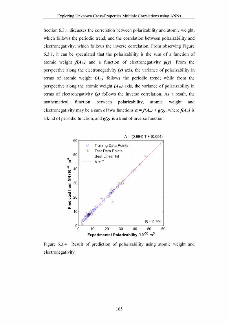
Exploring Unknown Cross-Properties Multiple Correlations using ANNs
165
Section 6.3.1 discusses the correlation between polarizability and atomic weight,
which follows the periodic trend; and the correlation between polarizability and
electronegativity, which follows the inverse correlation. From observing Figure
6.3.1, it can be speculated that the polarizability is the sum of a function of
atomic weight f(AW) and a function of electronegativity g(χ). From the
perspective along the electronegativity (χ) axis, the variance of polarizability in
terms of atomic weight (AW) follows the periodic trend; while from the
perspective along the atomic weight (AW) axis, the variance of polarizability in
terms of electronegativity (χ) follows the inverse correlation. As a result, the
mathematical function between polarizability, atomic weight and
electronegativity may be a sum of two functions = f(Aw) + g(χ), where f(Aw) is
a kind of periodic function, and g(χ) is a kind of inverse function.
0 10 20 30 40 50 600
10
20
30
40
50
60
Experimental Polarizability /10-30 m3
Pre
dict
ed fr
om N
N /1
0-30 m
3
A = (0.994) T + (0.054)
R = 0.994
Au
Training Data PointsTest Data PointsBest Linear FitA = T
Figure 6.3.4 Result of prediction of polarizability using atomic weight and
electronegativity.
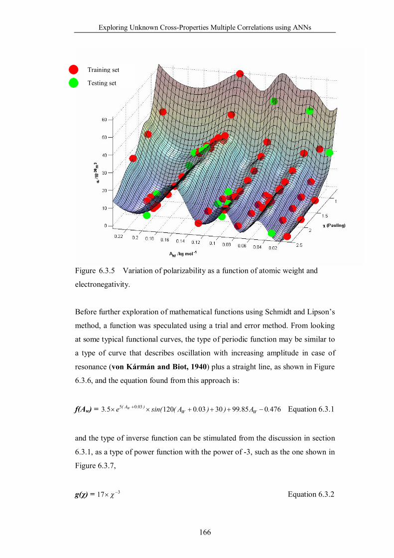
Exploring Unknown Cross-Properties Multiple Correlations using ANNs
166
Figure 6.3.5 Variation of polarizability as a function of atomic weight and
electronegativity.
Before further exploration of mathematical functions using Schmidt and Lipson’s
method, a function was speculated using a trial and error method. From looking
at some typical functional curves, the type of periodic function may be similar to
a type of curve that describes oscillation with increasing amplitude in case of
resonance (von Kármán and Biot, 1940) plus a straight line, as shown in Figure
6.3.6, and the equation found from this approach is:
f(Aw) = 476085993003012053 0305 .A.)).A(sin(e. WW).A( W Equation 6.3.1
and the type of inverse function can be stimulated from the discussion in section
6.3.1, as a type of power function with the power of -3, such as the one shown in
Figure 6.3.7,
g(χ) = 317 Equation 6.3.2
Training set
Testing set
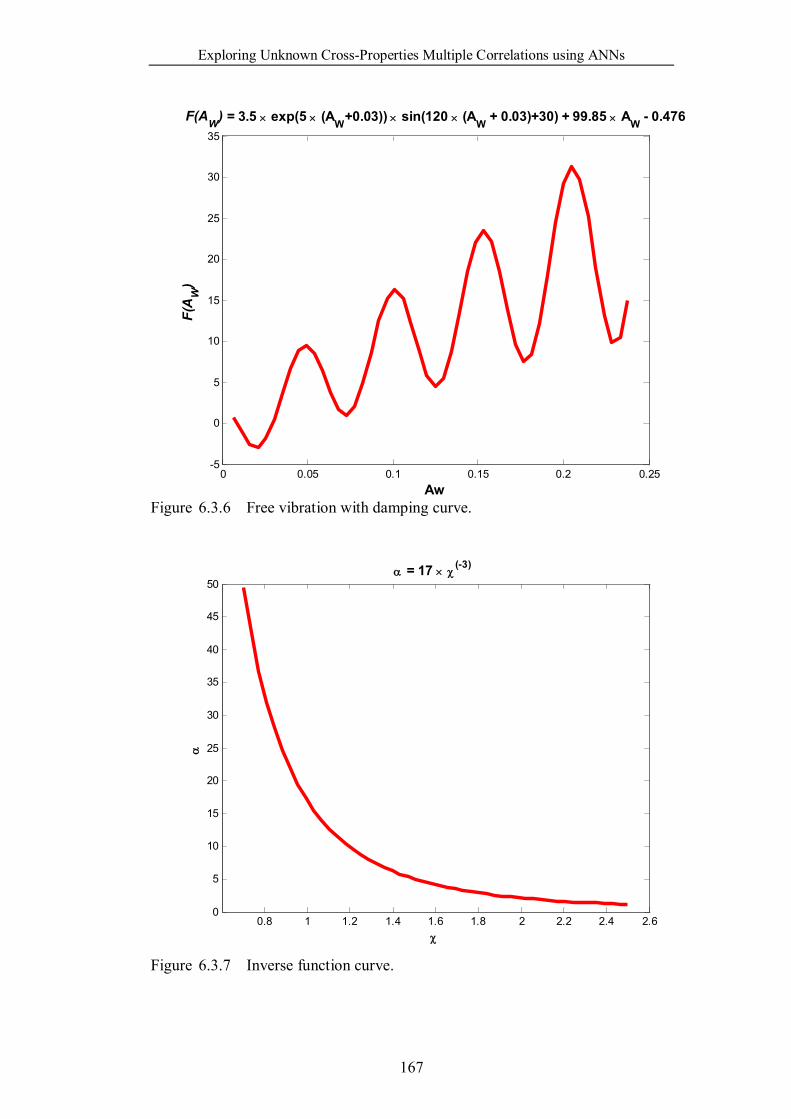
Exploring Unknown Cross-Properties Multiple Correlations using ANNs
167
0 0.05 0.1 0.15 0.2 0.25-5
0
5
10
15
20
25
30
35
Aw
F(A
W)
F(AW) = 3.5 exp(5 (AW+0.03)) sin(120 (AW + 0.03)+30) + 99.85 AW - 0.476
Figure 6.3.6 Free vibration with damping curve.
0.8 1 1.2 1.4 1.6 1.8 2 2.2 2.4 2.60
5
10
15
20
25
30
35
40
45
50 = 17 (-3)
Figure 6.3.7 Inverse function curve.
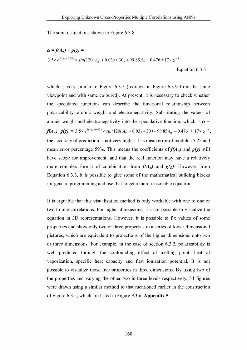
Exploring Unknown Cross-Properties Multiple Correlations using ANNs
168
The sum of functions shown in Figure 6.3.8
= f(Aw) + g(χ) =
476085993003012053 0305 .A.)).A(sin(e. WW).A( W + 317
Equation 6.3.3
which is very similar to Figure 6.3.5 (redrawn in Figure 6.3.9 from the same
viewpoint and with same coloured). At present, it is necessary to check whether
the speculated functions can describe the functional relationship between
polarizability, atomic weight and electronegativity. Substituting the values of
atomic weight and electronegativity into the speculative function, which is =
f(Aw)+g(χ) = 476085993003012053 0305 .A.)).A(sin(e. WW).A( W + 317 ,
the accuracy of prediction is not very high; it has mean error of modulus 5.25 and
mean error percentage 59%. This means the coefficients of f(Aw) and g(χ) still
have scope for improvement, and that the real function may have a relatively
more complex format of combination from f(Aw) and g(χ). However, from
Equation 6.3.3, it is possible to give some of the mathematical building blocks
for genetic programming and use that to get a more reasonable equation.
It is arguable that this visualization method is only workable with one to one or
two to one correlations. For higher dimensions, it’s not possible to visualize the
equation in 3D representations. However, it is possible to fix values of some
properties and show only two or three properties in a series of lower dimensional
pictures, which are equivalent to projections of the higher dimensions onto two
or three dimensions. For example, in the case of section 6.3.2, polarizability is
well predicted through the confounding effect of melting point, heat of
vaporization, specific heat capacity and first ionization potential. It is not
possible to visualize those five properties in three dimensions. By fixing two of
the properties and varying the other two in three levels respectively, 54 figures
were drawn using a similar method to that mentioned earlier in the construction
of Figure 6.3.5, which are listed in Figure A3 in Appendix 5.
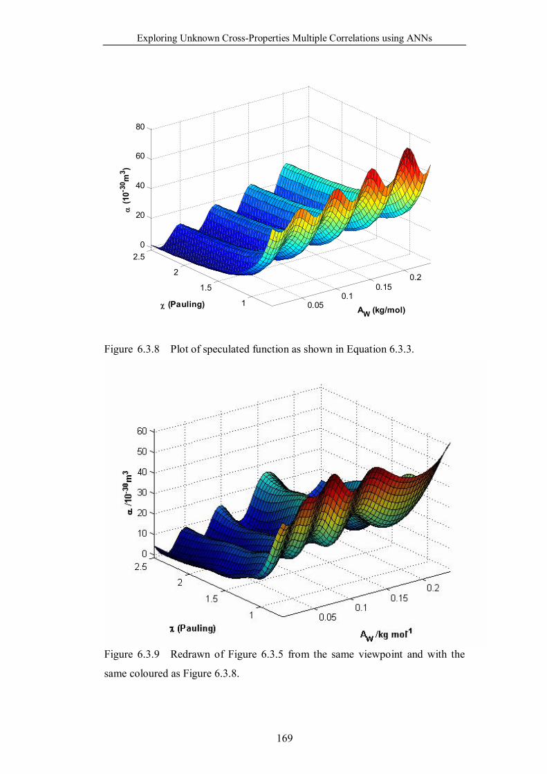
Exploring Unknown Cross-Properties Multiple Correlations using ANNs
169
0.050.1
0.150.2
1
1.5
2
2.50
20
40
60
80
AW (kg/mol) (Pauling)
(1
0-30 m
3 )
Figure 6.3.8 Plot of speculated function as shown in Equation 6.3.3.
Figure 6.3.9 Redrawn of Figure 6.3.5 from the same viewpoint and with the
same coloured as Figure 6.3.8.
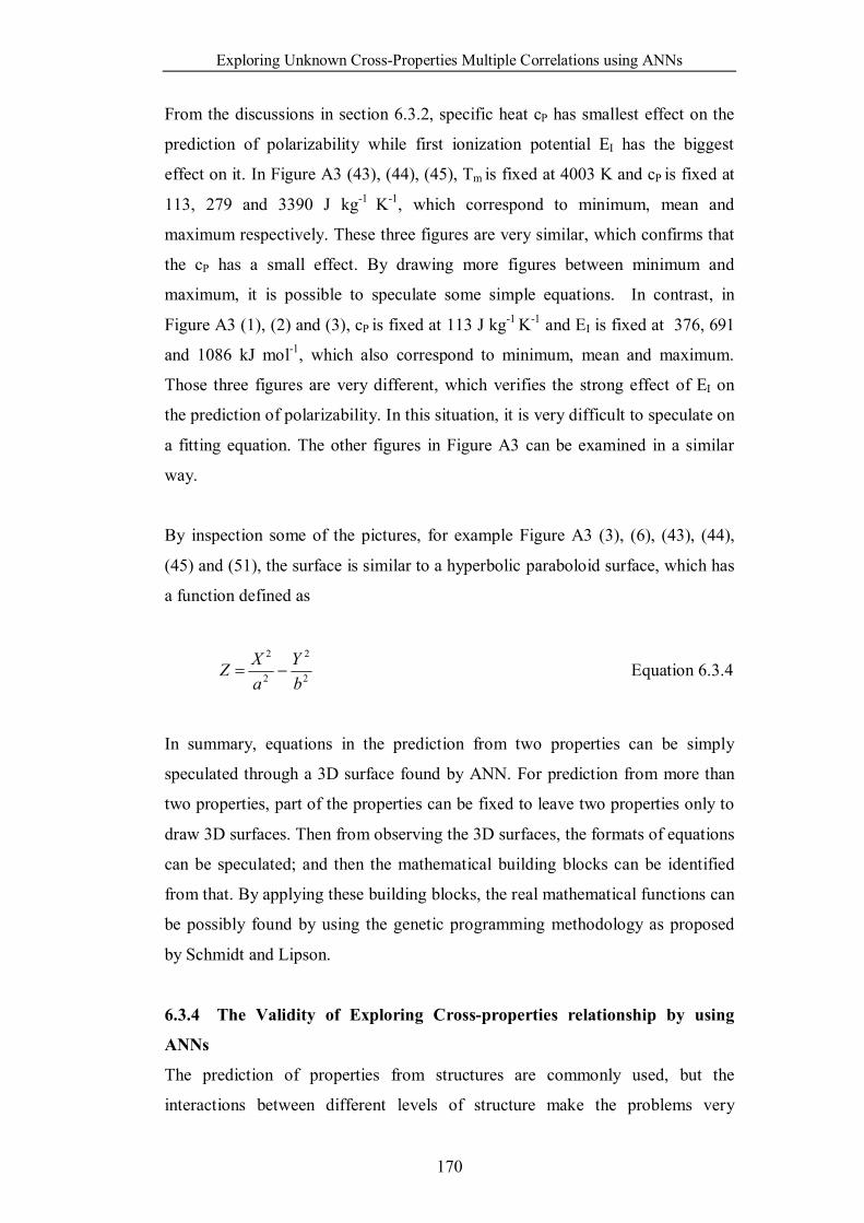
Exploring Unknown Cross-Properties Multiple Correlations using ANNs
170
From the discussions in section 6.3.2, specific heat cP has smallest effect on the
prediction of polarizability while first ionization potential EI has the biggest
effect on it. In Figure A3 (43), (44), (45), Tm is fixed at 4003 K and cP is fixed at
113, 279 and 3390 J kg-1 K-1, which correspond to minimum, mean and
maximum respectively. These three figures are very similar, which confirms that
the cP has a small effect. By drawing more figures between minimum and
maximum, it is possible to speculate some simple equations. In contrast, in
Figure A3 (1), (2) and (3), cP is fixed at 113 J kg-1 K-1 and EI is fixed at 376, 691
and 1086 kJ mol-1, which also correspond to minimum, mean and maximum.
Those three figures are very different, which verifies the strong effect of EI on
the prediction of polarizability. In this situation, it is very difficult to speculate on
a fitting equation. The other figures in Figure A3 can be examined in a similar
way.
By inspection some of the pictures, for example Figure A3 (3), (6), (43), (44),
(45) and (51), the surface is similar to a hyperbolic paraboloid surface, which has
a function defined as
2
2
2
2
bY
aXZ Equation 6.3.4
In summary, equations in the prediction from two properties can be simply
speculated through a 3D surface found by ANN. For prediction from more than
two properties, part of the properties can be fixed to leave two properties only to
draw 3D surfaces. Then from observing the 3D surfaces, the formats of equations
can be speculated; and then the mathematical building blocks can be identified
from that. By applying these building blocks, the real mathematical functions can
be possibly found by using the genetic programming methodology as proposed
by Schmidt and Lipson.
6.3.4 The Validity of Exploring Cross-properties relationship by using
ANNs
The prediction of properties from structures are commonly used, but the
interactions between different levels of structure make the problems very

Exploring Unknown Cross-Properties Multiple Correlations using ANNs
171
complex. In this work, apply the principle that the properties of a material are
determined by (or are a common response from) composition and structure, to
explore correlation between different properties by using artificial neural
networks. However, the interactions between input properties still exist. In neural
networks, the nature of the interactions is implicit in the values of the weights. In
cases like this work, there exist more than just pairwise interactions. As a result,
it is difficult to visualize from the examination of the weights. As suggested by
Bhadeshia (1999), the better method is to use the network to make predictions
and to see how these depend on various combinations of inputs. In this work, it is
tried to use the underlying physical principles to explain the different results and
found employing neural network to explore the cross-properties relationship is
reasonable.
The Feasibility of using ANN Methods
172
7.0 The Feasibility of using ANN Methods 7.1 The Validity of ANN Models
From all of the works presented above, it can be concluded that: the ANN, as a
method, can be treated as feasible although it cannot be relied on definitively and
others also have reiterated this. It may be regarded as a useful tool for cautious
use in materials science but the choice of the right ANN plays a critical role in its
success especially when the dataset is restricted as is often the case in materials
science.
7.2 The Effect of Number of Layers
Basheer and Hajmeer (2000) indicate that the choice of the number of hidden
layers and the number of neurons in the hidden layers are among the most
important choices in ANN design. Most of the works presented in this work are
function approximation problems. It is often claimed that in most function
approximation problems, one hidden layer is sufficient to approximate
continuous functions (Hecht-Nielsen, 1990; Basheer, 2000); two hidden layers
must generally be necessary for learning functions with discontinuities (Masters,
1993). In this work, the kind of function is not clear. Also the neural network
user’s guide (Mathworks) suggested that a two-hidden layers sigmoid/linear
network can represent any function of input/output relationship. On these bases
and looking at the results produced from all of the works, it can be seen that the
choice of two-hidden layer network is a sensible choice.
7.3 The Effect of Size of Layer
The choice of size of the first hidden layer is critical in the ANN design. There
are several rules of thumb available in the literature relating hidden layer size to
the number of nodes in input (NINP) and output (NOUT) layers:
Hecht-Nielsen (1990) used the Kolmogrov theorem to prove that NHN≤NINP
+1.
Widrow and Lehr (1990) according to (NW/NOUT)≤NTRN≤(NW/NOUT)
Log2(NW/NOUT).
Upadhaya and Eryureka (1992) related NHN to NTRN (via the total number
of weights, NW) according to NW = NTRN Log2(NTRN).

The Feasibility of using ANN Methods
173
Masters (1994) suggests that the ANN architecture should resemble a
pyramid with NHN≈(NINP * NOUT)1/2.
Lachtermacher and Fuller (1995) suggest the NHN for a one-output ANN
with no biases be determined from 0.11 NTRN≤NHN(NINP +1)≤0.30 NTRN.
Jadid and Fairbairn (1996) called for an upper bound on the number of hidden
nodes (NHN) equal to NTRN/[R+(NINP + NOUT)], where NTRN is the number of
training patterns and R=5-10.
As Basheer and Hajmeer (2000) suggested, the most popular way to find the
optimal number of hidden nodes is by trial and error with one of those rules as a
starting point. However, facing exotic problems with high nonlinearity and
hysteresis such as shown in Basheer’s work (Basheer, 1998; 2000), these ‘rules
of thumb’ may need to be abandoned. There is some value in beginning with a
small number of hidden nodes and building up iteratively to attain the accuracy
required. This method is adopted in all of the works through implementation of
the programs.
Conclusions
174
8.0 Conclusions 1. Revisiting Hume-Rothery’s Rules
Selection of Input Parameters
In this work, the input parameters initially chosen for the network include (1)
atomic size parameter, (2) valence parameter, (3) electrochemical parameter, i.e.
electronegativity and (4) structure parameter of solvent and solute atoms. Three
different expressions of these parameters were used to examine which gave the
best performance:
1. The raw data that Hume-Rothery used.
2. The original collected values for each parameter of solvent and solute
atoms.
3. The functionalized parameters.
When the raw data were used, uncertainty is the atomic size difference: some
researchers believe the threshold is 14% and others believe it is 15%. The
performance of ANN using the 15% criterion is slightly higher than that for 14%
which implies 15% is a better threshold in the size factor. Using this same
approach and including the 15% criterion, the structure parameter was introduced
in terms of whether the structure of solvents and solutes are the same or not.
There was no improvement in correlation. This indicates that the structure
parameter employed in this way, does not play a very important role in solubility.
When the original values of input parameters are used, the training performance
of the ANN is quite good but the prediction of the testing set is poor, and this
clearly indicates that although the network trains satisfactorily on the actual
values of input data it is unable to use these for prediction.
When the functionalized values were used as input parameters, both the training
and testing set of the ANN gave good performances. Through a search of all
combinations of those parameter formats, the best format of input parameters
was determined as the functionalized values.
Conclusions
175
Selection of Output Parameters
From Hume-Rothery’s Rules, only the possibility of whether a component is
soluble or insoluble can be predicted. However, it would be more advantageous
to attempt to predict the original value of solubility. The output parameters are
expressed in two ways:
1) Follow a specialized criterion: if the solubility of solute metal in solvent
metal exceeds 5 at. %, then it is said that this solute metal is soluble in the
solvent metal; or it is not.
2) Original maximum solubility limits of each alloy system are used: the results
of the prediction show the ANN can predict the solubility quantitatively with
small mean modulus errors for 60 alloy systems.
Testing Hume-Rothery’s Rules for 60 Alloy Systems
When the 60 alloy systems, which were used by Hume-Rothery, are tested, the
rules really work well as demonstrated by the ANN correlations. These indicate
the Hume-Rothery’s general principles work well in several alloy systems, and
can be used to estimate solid solubility.
Extension of Hume-Rothery’s Rules for 408 Alloy Systems
The wider application of the same approach to a set of 408 silver, copper and
gold alloys is less successful, and the predictability is poor. This is consistent
with the inherent simplifications of the rules which are already documented by
many people.
The Effect of Melting Point
Within a wider range of alloy systems, the introduction of melting point provides
the capability for improving the predictability: it can be treated as a new
parameter for solid solubility prediction. The prediction of Tmax, under which the
maximum solubility is reached, also confirms the effect of melting point.
Determination of the Relative Importance of Each Rule
In this work, the performance of the ANN, based on 60 alloy systems, was
evaluated when some of the parameters were deliberately omitted. Using the
Conclusions
176
mean error of the testing set as the main criterion for accuracy of the prediction,
atomic size has the strongest effect. Electronegativity has a stronger influence
than valence. When pairs of parameters are omitted, the performance of the
prediction became worse. Omission of the structure parameter only had small
effect on the performance of the ANN, which implies that the structure parameter
does not play a very important role. However, these parameters are not wholly
independent of each other; their interplay makes the determination of solubility
very difficult.
2. The Policing and Correction of Handbooks and Databases
In this work, it is found there were 21 elements having inconsistent boiling point
recording at the 10% level or above; and 23 elements having inconsistent
enthalpy of vaporization at the 10% level or above in five handbooks. These are
not trivial numbers in only 82 elements inspected.
Employed both boiling points and enthalpies of vaporization that having
consistent recording to train two ANNs (ANN1 and ANN2) provides a robust
correlation against which the consistency of other data can be judged. Applying
ANN1 to predict the enthalpies of vaporization of elements that have consistent
recordings of boiling points, made the average error decrease from 231% to 8.8%.
Then applying ANN2 to predict boiling points of elements that have consistent
recordings of enthalpy of vaporization made the average error decrease from
18.9% to 6.43%. For the elements that have inconsistent records of both boiling
point and enthalpy of vaporization, possible pairs have been found.
Compared with the statistical method adopted by Ashby et al., the method
developed locates more inconsistencies.
Extending the developed method to the more general situations (that is, more
than two properties correlated), a systematic, intelligent and potentially
automatic protocol has been developed to discover errors in handbooks. It could
be imported as an immune system. It involves the collection of data and
automatic exploration of indirect correlations within the data using ANNs.
Conclusions
177
3. The Prediction of Structural Stability and Formability of ABO3-type
Perovskite Compounds
In this part of work, 1) a neural network modelling method is used to make
predictions of global instability index GII from bond-valence based tolerance
factors tBV for 232 ABO3-type perovskite compounds and it is found that
correlations exist between these two parameters within each subclass of ABO3-
type perovskite compounds; for the general ABO3-type perovskite, this kind of
correlation is not obeyed. However, it was found that the valence of A-site
cations can be treated as another parameter to induce a unified correlation. 2)
Neural networks have also been used to make predictions of formability of
perovskites by using A-O and B-O bond distances in order to find the possibility
of improving prediction accuracy. It was found that, in terms of the prediction
accuracy, neural networks can yield better performances, although it is difficult
to give simple and physically meaningful explanations.
4. Correlation between Polarizability and Other Properties
In this work, the general correlations that exist between different properties are
explored by employing artificial neural network methods. The example of
prediction of polarizability from combinations of other properties is analyzed in
detail. Through this work, a systematic method for exploring general correlations
that exist between different properties for different type of materials is provided.
1) It has been found that there are four properties that have single relatively
strong correlations with polarizability. They are atomic weight, first ionization
potential, electronegativity and work function. The underlying physical
principles have been discussed individually.
2) The correlation between polarizability and combinations of melting point, heat
of vaporization, first ionization potential and specific heat has been found, and
the possible confounding effects are systematically analysed.
3) The prediction of polarizability from atomic weight and electronegativity is
analysed as an example to visualize the functional relationship that neural
network captured, and the surface that describes the variation of polarizability as
Conclusions
178
a function of atomic weight and electronegativity has been schematically shown.
The possible mathematical equation that formulates and generalizes the
correlation has been explored by a trial and error method, which could provide
building blocks for generic programming.
4) For the case mentioned in 2), the neural network captured the correlation
between polarizability and another four different properties. However, it is
difficult for people to visualize this kind of functional correlation directly, which
is located within a 5-D space. By fixing two of the properties and varying the
other two in three levels respectively, a series of figures have been drawn in
order to visualize this high dimensional function from its projection within a 3-D
space. Also, relative impact of each parameter was verified.
Future Works
179
9.0 Suggestions for Future Work 1. Verifying and Testing Hume-Rothery’s Rules
Although Hume-Rothery’s rules were tested at the beginning of this project to
prove the ability of ANNs in finding known correlations in materials science, a
few interesting directions have been identified from this section which can be
investigated in future:
A better way to express structures of elements for the input parameters of
ANNs should be explored, for example, 1) find expressions that can reveal the
similarities between FCC and HCP; 2) get some special expressions that can
describe complex structures. These will help not only the proof of H-R rules
but also other areas that use crystal structures as input parameters in materials
science by using artificial intelligence.
From the handbooks as mentioned in this work, such as the ASM Handbook,
Alloy Phase Diagrams, Binary Phase Diagrams and Chemistry Data Book, it
would be possible to draw together solubilities and physical parameters for
more alloy systems for training and testing Hume-Rothery’s Rules.
It would be constructive and valuable to try to find other parameters that may
affect the solid solubility of alloy systems and then to introduce them to the
neural network for predicting the solid solubility limit of alloy systems. This
could be done by introducing other properties such as pressure, cooling rate,
and then use a combinatorial search of those properties by ANNs.
2. Policing Data with more than Two Correlating Properties
In this part of the work, a systematic method has been proposed to detect errors
in handbooks. Following this trend, more properties should be progressively
introduced to verify this general methodology. The method should then be
applied for a wider range of databases. This forms a natural part of the project in
investigating the cross property correlation method of discovery for without
reliable data the correlations could not be discovered, and once the correlations is
discovered, the outliers can be screened by ANNs.
Future Works
180
3. Prediction of formability of ABO3-type perovskite compounds by using
more input parameters
Neural networks have the ability to make predictions in high dimensional spaces,
i.e., they can have more than two inputs to make the prediction. For the
prediction of formability of ABO3-type perovskite compounds, as mentioned by
Zhang et al. (2007), besides the A-O and B-O bond distances, other factors also
contribute to the formation of ABO3-type perovskite compounds, such as i)
bond-valence based tolerance factor tBV, ii) temperature and iii) pressure;
therefore, these parameters can be incorporated into future work in order to
improve the accuracy of predictions, which can be used for practical applications.
4. Exploration of Cross Property Correlations with more data
The method applied in the exploration of cross-property correlations depends
strongly on the available data. At present, the advent of e-science has meant that
scientific communication can employ media not previously recognized. Data can
be made accessible globally so that many geographically dispersed groups can
analyze raw data according to their own skills. As a result, the sharing of data in
raw form rather than through the highly processed medium of refereed journals is
now possible. This means that the construction of global shared databases is a
reality and it follows from that, multi-property data can be put up and shared.
There are varieties of databases available, such as the ones listed by Wawrousek
et al. (1989). Nowadays, more and more of these databases can be accessed via
the internet (Westbrook et al., 1995; Abrate, 2000). One recent example is the
functional ceramic materials database developed by Scott et al. (2008).
After the data sharing is in place, the computational processes for mining the
relationships are needed. Methods are required to develop for identifying how the
measurement of properties a, b and c can be used to estimate the likely
magnitude of property d. This will considerable narrow down the likely sample
space for high throughput methods for d and, as the global database grows this
cross-correlation may produce a new area of materials science that allows the
scientific world to home in on new materials at a rate previously thought
impossible. Where high throughput methods have compressed laboratory time,
multi-property mapping might compress the history of science.
References
181
References Abe T., Sundman B., Onodera H. Thermodynamic assessment of the Cu-Pt
system. Journal of Phase Equilibria and Diffusion. 2006, 27, 5-13.
Abrate S. World Wide Web resources for materials science. Computer
Applications in Engineering Education. 2002, 9, 238-247.
Ackland G. J., Vitek V. Many-body potentials and atomic-scale relaxations in
noble-metal alloys. Physical Review B. 1990, 41, 10324-10333.
Agren J. Calculation of phase diagrams: Calphad. Current Opinion in Solid
State and Materials Science. 1996, 1, 355-360.
Agyemang M., Barker K., Alhajj R. A comprehensive survey of numeric and
symbolic outlier mining techniques. Intelligent Data Analysis. 2006, 10, 521-538.
Allen F. H. The development, status and scientific impact of crystallographic
databases. Acta Crystallographica. 1998, A54, 758-771.
Alonso J. A., Girifalco L. A. Non-locality and the energy of alloy formation.
Journal of Physics F – Metal Physics. 1978, 8, 2455-2460.
Alonso J. A., Girifalco L. A. Electronegativity scale for metals. Physical Review
B. 1979, 19, 3889-3895.
Alonso J. A., Gonzalez D. J., Iniguez M. P. Electronegativity parameters of the
theory of heats of alloy formation. Solid State Communications. 1979, 31, 9-14.
Alonso J. A., Simozar S. Prediction of solid solubility in alloys. Physical
Review. 1980, B22, 5583-5589.
Alonso J. A., Lopez J. M. Semi-empirical study of metastable alloys produced
by ion-implantation in metals. Philosophical Magazine A – Physics of
Condensed Matter Structure Defects and Mechanical Properties. 1982, 45, 713-
722.
Alonso J. A., Lopez J. M., Simozar S., Girifalco L. A. Prediction of solid
solubility in alloys – Application to noble metal based alloys. Acta Metallurgica.
1982, 30, 105-107.

References
182
Amari S. Foreword to neural networks theory. In: Galushkin, A. I. Neural
Network theory. Springer Berlin Heidelberg New York, 2007, p. X.
American Society for Metals. ASM handbook / Vol.3, Alloy phase diagrams.
Metals Park, Ohio: ASM International, 1992, pp.2.25-2.182.
Amis E. J., Xiang X. D., Zhao J. C. Combinatorial materials science: what’s
new since Edison? MRS Bulletin. 2002, 27, 295-297.
Ansara I., Dinsdale A. T., Rand M. H. (Eds). COST 507 – Thermochemical
database for light metal alloys, Vol. 2. European Cooperation in the Field of
Scientific and Technical Research, 1998.
Apker L., Taft E., Dickey J. Photoelectric emission and contact potentials of
semiconductors. Physical Review. 1948, 74, 1462-1474.
Arblaster J. W. The thermodynamic properties of platinum. Platinum Metals
Review. 2005, 49, 141-149.
Arblaster, J. W. Vapour pressure equations for the platinum group elements.
Platinum Metals Review. 2007, 51, 130-135.
Arkadan A. A., Chen Y., Subramaniam S., Hoole S. R. H. NDT identification
of a crack using ANNs with stochastic gradient descent. IEEE Transactions on
Magnetics. 1995, 31, 1984-1987.
Arroyave R., Kaufman L., Eagar T. W. Thermodynamic modelling of the Zr-
O system. CALPHAD. 2002, 26, 95-118.
Ashby M. F. Overview No. 80. On the engineering properties of materials. Acta
Metallurgica. 1989, 37, 1273-1293.
Ashby M. F. Checks and estimates for material properties I. Ranges and simple
correlations. Proceedings of the Royal Society of London A – Mathematical
Physical and Engineering Sciences. 1998, 454, 1301-1321.
Ashby M. F. Materials Selection in Mechanical Design. Oxford: Butterworth-
Heinemann, 1999. pp. 32-64.
References
183
Ashby M. F., Shercliff H., Cebon D. Materials: Engineering, Science,
Processing and Design. Butterworth-Heinemann, Elsevier: 2007, pp. 22-24, 58-
59.
Asta M., Ozolins V., Woodward C. A first-principles approach to modelling
alloy phase equilibria. JOM – Journal of the Minerals Metals & Materials
Society. 2001, 53, 16-19.
Atoji M. Atomic polarizability. The Journal of Chemical Physics. 1956, 25, 174.
Attoh-Okine N. O., Basheer I. A., Chen D. -H., Abu-Lebdeh G., McReynolds
R., Meier R., Najjar Y. M., Penumadu D., Tutumluer E. Use of artificial
neural networks in geomechanical and pavement systems. Transportation
Research Board, National Research Council, 2101 Constitution Avenue, NW,
Washington, DC 20418. Circular, Dec. 1999. 21 pages. No. E-C012, ISSN 0097-
8515.
Axon H. J., Hume-Rothery W. The lattice spacings of solid solutions of
different elements in aluminium. Proceedings of the Royal Society of London, A.
Mathematical and Physical Sciences. 1948, 193, 1-24.
Aylward G., Findlay T., ed. SI Chemical Data, 4th edn. New York; Chichester:
Wiley, 1998, pp.6-13.
Bacalis N. C., Anagnostopoulos G. F., Papanicolaou N. I.,
Papaconstantopoulos D. A. Electronic structure of ordered and disordered Cu-
Ag alloys. Physical Review B. 1997, 55, 2144-2149.
Bacon F. (Ellis R. L., Spedding J., Robertson J. M. (Eds.)). Novum Organum in
The Philosophical Works of Francis Bacon. Routledge Abingdon, UK 1905.
Bagnall, K. W. The Chemistry of Selenium, Tellurium and Polonium.
Amsterdam; New York: Elsevier, 1966. pp. 37-38.
Baranyi J., Roberts T. A. Mathematics of predictive food microbiology.
International Journal of Food Microbiology. 1995, 26, 199-218.
Basheer I. A. Neuromechanistic-based modeling and simulation of constitutive
behavior of fine-grained soils. PhD Dissertation, Kansas State University,
Manhattan; 1998. 435p.
References
184
Basheer I. A. Selection of methodology for neural network modeling of
constitutive hystereses behavior of soils. Computer – Aided Civil and
Infrastructure Engineering. 2000, 15, 440-458.
Basheer I. A., Hajmeer M. Artificial neural networks: fundamentals, computing,
design, and application. Journal of Microbiological Methods. 2000, 43, 3-31.
Bassetti D., Brechet Y., Ashby M. F. Estimates for material properties II. The
method of multiple correlations. Proceedings of the Royal Society of London A –
Mathematical Physical and Engineering Sciences. 1998, 454, 1323-1336.
Bedreag C. G. Electron extraction potential of alkali metals. Comptes Rendus.
1946, 223, 354-354.
Ben-Gal I. Outlier detection. In: Maimon O., Rokach L. (Eds.) Data Mining
and Knowledge Discovery Handbook. Springer: New York. 2005. pp. 131-146.
Bergerhoff G., Hundt R., Sievers R. The Inorganic Crystal Structure Database.
Journal of chemical information and computer sciences. 1983, 23, 66-69.
Bhadeshia H. K. D. H. A rationalisation of shear transformations in steels. Acta
Metallurgica. 1981, 29, 1117-1130.
Bhadeshia H. K. D. H., MacKay D. J. C., Svensson L. –E. Impact toughness
of C-Mn steel arc welds – Bayesian neural network analysis. Materials Science
and Technology. October 1995, 11, 1046-1051.
Bhadeshia H. K. D. H. Neural networks in materials science. ISIJ International.
1999, 39, 966-979.
Bhadeshia H. K. D. H. Mathematical models in materials science. Materials
Science and Technology. 2008, 24, 128-136.
Bhadeshia H. K. D. H. Neural networks and information in materials science.
Statistical Analysis and Data Mining. 2009, 1, 296-305.
Bhadeshia H. K. D. H., Dimitriu R. C., Forsik S., Pak J. H., Ryu J. H.
Performance of neural networks in materials science. Materials Science and
Technology. 2009, 25, 504-510.
References
185
Bishop C. M. Novelty detection and neural network validation. IEE Proceedings
– Vision Image and Signal Processing. 1994, 141, 217-222.
Blum V., Zunger A. Structural complexity in binary bcc ground states: The case
of bcc Mo-Ta. Physical Review B. 2004, 69, 020103(1)-020103(4).
Bonin K. D., Kresin V. V. Electric-Dipole Polarizabilities of Atoms, Molecules
and Clusters. Singapore: World Scientific Publishing Co. Pte. Ltd. 1997.pp. vii-
viii.
Boozarjomehry R. B., Abdolahi F., Moosavian M. A. Characterization of
basic properties for pure substances and petroleum fractions by neural network.
Fluid Phase Equilibria. 2005, 231, 188-196.
Borie B. S. X-ray diffraction effects of atomic size in alloys. Acta
Crystallographica. 1957, 10, 89-96.
Borie B. S. X-ray diffraction effects of atomic size in alloys II. Acta
Crystallographica. 1959, 12, 280-282.
Bork U., Challis R. E. Non-destructive evaluation of the adhesive fillet size in a
T-peel joint using ultrasonic Lamb waves and a linear network for data
discrimination. Measurement Science and Technology. 1995, 6, 72-84.
Borman S. Combinatorial chemistry: researchers continue to refine techniques
for identifying potential drugs in “libraries” of small organic molecules.
Chemical & Engineering News. 1997, February 24, 43-62.
Borzone G., Parodi N., Cacciamani G., Watson A. Phase equilibria in the Au-
In-Sn ternary system. CALPHAD. 2009, 33, 17-22.
Bouwstra J. A., Geels G., Kaufman L., Oonk H. A. J. Binary common-ion
alkali halide mixtures thermodynamic analysis of solid-liquid phase diagrams IV.
Three systems showing isodimorphism application of the liqfit method.
CALPHAD. 1986, 10, 163-174.
Bozzolo G., Ferrante J. Heats of formation of bcc binary alloys. Physical
Review B. 1992, 45, 12191-12197.
Bozzolo G., Ferrante J., Smith J. R. Method for calculating alloy energetics.
Physical Review B. 1992, 45, 493-496.
References
186
Bozzolo G., Noebe R. D., Ferrante J., Amador C. An introduction to the BFS
method and its use to model binary NiAl alloys. Journal of Computer-Aided
Materials Design. 1999, 6, 1-32.
Bragg W. L. The structure of some crystals as indicated by their diffraction of
X-rays. Proceedings of the Royal Society of London, Series A. 1913, 89, 248-277.
Bratchell N., Mcclure P. J., Kelly T. M., Roberts T. A. Predicting microbial-
growth – graphical methods for comparing models. International Journal of
Food Microbiology. 1990, 11, 279-287.
Brooks H. Binding in metals. Transactions of the Metallurgical Society of AIME.
1963, 227, 546-560.
Brooks L. S. The vapor pressure of tellurium and selenium. Journal of the
American Chemical Society. 1952, 74, 227-229.
Brugger P. From haunted brain to haunted science: a cognitive neuroscience
view of paranormal and pseudoscientific thought. In: Houran J., Lange R.
(Eds.) Hauntings and Poltergeists: Multidisciplinary Perspectives. North
Carolina: McFarland & Company, Inc. 2001. pp. 195-213.
Buckley R. A., Hume-Rothery W. The liquid → solid and δ → γ equilibria in
iron-rich alloys. Journal of the Iron and Steel Institute. 1963, 201, 227-232.
Burdett J. K., Rodgers J. R. Structure & property maps for inorganic solids. In:
King R. B. (ed.), Encyclopedia of Inorganic Chemistry, Vol. 7, John Wiley &
Sons, New York, 1994. pp. 1-19.
Cachadiña I., Mulero A. Vaporization enthalpy: corresponding-states
correlations versus DIPPR database. Journal of Physical and Chemical
Reference Data. 2007, 36, 1133-1139.
Cai K., Xia J., Li L., Gui Z. Analysis of the electrical properties of PZT by a BP
artificial neural network. Computational Materials Science. 2005, 34, 166-172.
Callister W. D., Jr. Materials Science and Engineering: An Introduction. 6th edn.
John Wiley & Sons, Inc., New York, 2003. pp. 2-3, 658-659.
References
187
Cao Z. M., Takaku Y., Ohnuma I., Kainuma R., Zhu H. M., Ishida K.
Thermodynamic assessment of the Ni-Sb binary system. Rare Metals. 2008, 27,
384-392.
Cargnoni F., Gatti C., Colombo L. Formation and annihilation of a bond defect
in silicon: an ab initio quantum-mechanical characterization. Physical Review B.
1998, 57, 170-177.
Cawse J. N. The Combinatorial Challenge. In: Cawse J. N. (Eds). Experimental
design for combinatorial and high throughput materials development. John
Wiley & Sons, Inc., Hoboken, New Jersey, 2003. pp. 1-26.
CES EduPack 2008. Cambridge Engineering Selector. Granta Design Ltd.,
Rustat House, 62 Clifton Court, Cambridge CB1 7EG, UK.
www.grantadesign.com
Chalk A. J., Beck B., Clark T. A quantum mechanical/neural net model for
boiling points with error estimation. Journal of Chemical Information and
Computer Sciences. 2001, 41, 457-462.
Chan P. K., Fan W., Prodromidis A. L., Stolfo S. J. Distributed data mining in
credit card fraud detection. IEEE Intelligent Systems & Their Applications. 1999,
14, 67-74.
Chang Y. A., Chen S., Zhang F., Yan X., Xie F., Schmid-Fetzer S., Oates W.
A. Phase diagram calculation: past, present and future. Progress in Materials
Science. 2004, 49, 313-345.
Chelikowsky J. R., Phillips J. C. Quantum-defect theory of heats of formation
and structural transition energies of liquid and solid simple metal alloys and
compounds. Physical Review B. 1978, 17, 2453-2477.
Chelikowsky J. R. Solid solubilities in divalent alloys. Physical Review. 1979,
B19, 686-701.
Chelikowsky J. R. Microscopic basis of Miedema’s theory of alloy formation.
Physical Review B. 1982, 25, 6506-6508.
Chelikowsky J. R. Cohesive energy. In: Encyclopedia of Applied Physics.
Weinheim: Wiley-VCH. 2004. p. 260.
References
188
Chen N. H. Generalized correlation for latent heat of vaporization. Journal of
Chemical and Engineering Data. 1965, 10, 207-210.
Chen S. W., Jan C. H., Lin J. C., Chang Y. A. Phase equilibria of the Al-Li
binary system. Metallurgical and Materials Transactions A. 1989, 20, 2247-2258.
Chen S. L., Chang Y. A. A thermodynamic analysis of the Al-Zn system and
phase diagram calculation. CALPHAD. 1993, 17, 113-124.
Chin J., Harting J., Jha S., Coveney P. V. Steering in computational science:
mesoscale modelling and simulation. Contemporary Physics. 2003, 44, 417-434.
Chrisman N. R. The error component in spatial data. In Maguire D. J.,
Goodchild M.F. and Rhind D. W. (Eds.) Geographical Information Systems.
Vol. 1: Principals. John Wiley & Sons, New York, 1991. pp. 165-174.
Chuang Y. Y., Hsieh K. C., Chang Y. A. Thermodynamics and phase
relationships of transition metal-sulfur systems: Part V. A reevaluation of the Fe-
S system using an associated solution model for the liquid phase. Metallurgical
and Materials Transactions B. 1985, 16, 277-285.
Chuang Y. Y., Chang Y. A., Schmid R., Lin J. C. Magnetic contributions to
the thermodynamic functions of alloys and the phase equilibria of Fe-Ni system
below 1200 K. Metallurgical and Materials Transactions A. 1986, 17, 1361-
1372.
Chuang Y. Y., Chang Y. A. A thermodynamic analysis and calculation of the
Fe-Ni-Cr phase diagram. Metallurgical and Materials Transactions A. 1987, 18,
733-745.
Clark C. H. D. Spectroscopy and valency. II. The periodic groups of nonhydride
diatomic molecules. Proceedings of the Leeds Philosophical and Literary Society.
1934, 2, 502-512.
Cockayne B., Raynor G. V. The apparent metallic valencies of transition metals
in solid solution. Proceedings of the Royal Society of London. Series A,
Mathematical and Physical Sciences. 1961, 261, 175-188.
Colinet C., Pasturel A., Manh D. N., Pettifor D. G., Miodownik P. Phase-
stability study of the Al-Nb system. Physical Review B. 1997, 56, 552-565.
References
189
Colinet C. Ab-initio calculation of enthalpies of formation of intermetallic
compounds and enthalpies of mixing of solid solutions. Intermetallics. 2003, 11,
1095-1102.
Colliez J., Dufrenois F., Hamad D. Robust regression and outlier detection with
SVR: application to optic flow estimation. The 17th British Machine Vision
Conference. 2006. Edinburgh. 10 pages. (Entry website, on 22/10/2009:
http://www.macs.hw.ac.uk/bmvc2006/papers/446.pdf)
Condon E. U. Note on the external photoelectric effect of semi-conductors.
Physical Review. 1938, 54, 1089-1091.
Constantinou L., Gani R. New group contribution method for estimating
properties of pure compounds. AIChE Journal. 1994, 40, 1697-1710.
Cottrell A. An introduction to metallurgy. London: Edward Arnold. 1975. pp.
345-347.
Cottrell A. Concepts in the electron theory of alloys. London: IOM
Communications; 1998. pp. 27-102.
Cui Y., Jin Z. Assessment of the Re-Ta binary system. Journal of Alloys and
Compounds. 1999, 285, 150-155.
Curtarolo S., Morgan D., Persson K., Rodgers J., Ceder G. Predicting crystal
structures with data mining of quantum calculations. Physical Review Letters.
2003, 91, 135503(1)-135503(4).
Curtarolo S., Morgan D., Ceder G. Accuracy of ab initio methods in predicting
the crystal structures of metals: A review of 80 binary alloys. CALPHAD. 2005,
29, 163-211.
Daane A. H. Physical properties of the rare-earth metals. In: Spedding F. H.,
Daane A. H. (Eds.) The Rare Earths. John Wiley & Sons, Inc.: New York and
London, 1961, pp. 177-189.
Dagani R. A faster route to new materials. Chemical & Engineering News. 1999,
77, 51-60.
Dainton, F. S., Kimberley, H. M. A radioactive tracer method for the
determination of the variation of vapour pressure with temperature and its
References
190
application to White Phosphorus. Transactions of the Faraday Society. 1950, 46,
912-918.
Dalcin E. C. Data quality concepts and techniques applied to taxonomic
databases. Thesis for the degree of Doctor of Philosophy. University of
Southampton. 2005, p.21.
Darken L. S., Gurry R. W. Physical Chemistry of Metals. New York: McGraw-
Hill. 1953. pp. 74-109.
David R. L. (Eds.) CRC Handbook of Chemistry and Physics. 2000-2001. 81st
edn. Boca Raton: CRC Press, c2000, p. (4)124, pp. (6)105-(6)106.
Debye P. Polar Molecules. New York: Chemical Catalog Company, Inc., 1929.
pp. 15-35.
De Chatel P. F., Robinson G. G. Formation energy of heterovalent alloys.
Journal of Physics F – Metal Physics. 1976, 6, L174-L176.
De Podesta, M. Understanding the Properties of Matter, 2nd edn. (Taylor &
Francis, London, 2001), p.344.
De Selincourt M. The boiling point of selenium. Proceedings of the Physical
Society. 1940, 52, 348-352.
Dean J. A. Lange’s Handbook of Chemistry, 12th edition. New York; London:
McGraw-Hill, 1979. p. (9-112).
Deibuk V. G., Dremlyuzhenko S. G., Ostapov S. E. Thermodynamic stability
of bulk and epitaxial CdHgTe, ZnHgTe, and MnHgTe alloys. Semiconductors.
2005, 39, 1111-1116.
Denbigh K. G. The polarisabiliuties of bonds-I. Transactions of the Faraday
Society. 1940, 36, 936-948.
Diaconis P., Mosteller F. Methods for studying coincidences. Journal of the
American Statistical Association. 1989, 84, 853-861.
Ding X. Y., Fan P., Wang W. Z. Thermodynamic calculation for alloy systems.
Metallurgical and Materials Transactions B – Process Metallurgy and Materials
Processing Science. 1999, 30, 271-277.
References
191
Disalvo F. J. Solid-state chemistry: a rediscovered chemical frontier. Science.
1990, 247, 649-655.
Dixon R. D., Lott L. A. Work function of ultrahigh-vacuum-deposited beryllium
films. Journal of Applied Physics. 1969, 40, 4938-4939.
Dmitrieva I. K., Plindov G. I. Dipole polarizability, radius and ionization
potential for atomic systems. Physica Scripta. 1983, 27, 402-406.
Dorsett H. and White A. Overview of molecular modeling and ab initio
molecular orbital methods suitable for use with energetic materials. Aeronautical
and Maritime Research Laboratory, Salisbury, Australia. Weapons Systems
Division, 2000. 36 pages. Report DSTO no. DSTO-GD-0253.
Drude P. Zur Elektronentheorie der Metalle. Annalen der Physik. 1900a, 306,
566-613.
Drude P. Zur Elektronentheorie der Metalle; II. Teil. Galvanomagnetische und
thermomagnetische Effecte. Annalen der Physik. 1900b, 308, 369-402.
Du Y., Clavaguera N. Thermodynamic assessment of the Al-Ni system. Journal
of Alloys and Compounds. 1996, 237, 20-32.
Du Z., Xu Y., Zhang W. Thermodynamic assessment of the Cu-La system.
Journal of Alloys and Compounds. 1999, 289, 89-95.
Du Z., Yang H., Li C. Thermodynamic modeling of the Pd-Y system. Journal of
Alloys and Compounds. 2000, 297, 185-191.
Du Z., Yang H. Thermodynamic assessment of the Gd-Pd system. Journal of
Alloys and Compounds. 2000, 312, 181-188.
Duhem P. Medieval Cosmology: Theories of Infinity, Place, Time, Void, and the
Plurality of Worlds. Chicago: University of Chicago, 1985. pp. 431-439.
Duschanek H., Rogl P., Lukas H. L. A critical assessment and thermodynamic
calculation of the boron-carbon-titanium [B-C-Ti] ternary system. Journal of
Phase Equilibria. 1995, 16, 46-60.
Eddington A. S. The Philosophy of Physical Science. Cambridge: University
Press, 1949, pp. 1-15.
References
192
Egolf L. M., Jurs P. C. Prediction of boiling points of organic heterocyclic
compounds using regression and neural network techniques. Journal of Chemical
Information and Computer Sciences. 1993, 33, 616-625.
Elsässer Ch., Fisher C. A. J., Howe A., Parrinello M., Scheffler M., and Gao
H. Introduction to Materials Theory and Modelling. In: European White Book on
Fundamental Research in Materials Science. Max-Planck-Institut für
Metallforschung Stuttgart, 2001. Chapter 4, Materials Theory and Modelling. pp.
126-128.
Emsley J. The Elements, 3rd edn. Oxford: Oxford University Press, 1998.
Eshelby J. D. The continuum theory of lattice defects. Solid State Physics. 1956,
3, 79-144.
European White Book on Fundamental Research in Materials Science. Max
– Planck – Institut für Metallforschung Stuttgart, 2001. p. 10.
Evans J. R. G., Edirisinghe M. J., Coveney P. V., Eames J. Combinatorial
searches of inorganic materials using the ink-jet printers: science, philosophy and
technology. Journal of the European Ceramic Society. 2001, 21, 2291-2299.
Falk R., Konold C. Making sense of randomness: implicit encoding as a basis
for judgment. Psychological Review. 1997, 104, 301-318.
Fan W. F., Geerts F., Jia X. B., Kementsietsidis A. Conditional functional
dependencies for capturing data inconsistencies. ACM Transactions on Database
Systems. 2008, 33, Article No. 6.
Fang F., Zeng M. Q., Che X. Z., Zhu M. Embedded atom potential calculation
of the Al-Pb immiscible alloy system. Journal of Alloys and Compounds. 2002a,
34, 252-255.
Fang S. S., Lin G. W., Zhang J. L., Zhou Z. Q. The maximum solid solubility
of the transition metals in palladium. International Journal of Hydrogen Energy.
2002a, 27, 329-332.
Fang F., Zeng M. Q., Che X. Z., Zhu M. Embedded atom potential calculation
of the Al-Pb immiscible alloy system. Journal of Alloys and Compounds. 2002b,
34, 252-255.
References
193
Fayyad U. M., Piatetsky-Shapiro G., Uthurusamy R. Summary from the
KDD-03 panel: data mining: the next 10 years. ACM SIGKDD Explorations
Newsletter. 2003, 5, 191-196.
Fedors R. F. A method for estimating both the solubility parameters and molar
volumes of liquids. Polymer Engineering and Science. 1974, 14, 147-154.
Feng L. M., Jiang L. Q., Zhu M., Liu H. B., Zhou X., Li C. H. Formability of
ABO3 cubic perovskites. Journal of Physics and Chemistry of Solids. 2008, 69,
967-974.
Fey N. Review organometallic molecular modeling – the computational
chemistry of metallocenes: a review. Journal of Chemical Technology and
Biotechnology. 1999, 74, 852-862.
Feynman R. P. What is science? In: The Physics Teacher, Vol 9. American
Association of Physics Teachers, 1969. pp. 313-320.
Fischer C. C., Tibbetts K. J., Morgan D., Ceder G. Predicting crystal structure
by merging data mining with quantum mechanics. Nature Materials. 2006, 5,
641-646.
Fish L. W., Lielmezs J. General method for predicting the latent heat of
vaporization. Industrial & Engineering Chemistry Fundamentals. 1975, 14, 248-
256.
Flandorfer H., Grobner J., Stamou A., Hassiotis N., Saccone A., Rogl P.,
Wouters R., Seifert H., Maccio D., Ferro R., Haidemenopoulos G., Delaey L.,
Effenberg G. Experimental investigation and thermodynamic calculation of the
ternary system Mn-Y-Zr. Zeitschrift Fur Metallkunde. 1997, 88, 529-538.
Flemings M. C. What next for departments of materials science and engineering?
Annual Review of Materials Research. 1999, 29, 1-23.
Fourier J. Théorie Analytique de la Chaleur, Par M. Fourier. A Paris, Chez
Firmin Didot, Père et Fils, Libraires Pour Les Mathématiques, L’architecture
Hydraulique et la Marine, Rue Jacob, No 24. 1822.
Franz R., Wiedemann G. Ueber die Wärme-Leitungsfähigkeit der Metalle.
Annalen der Physik und Chemie. 1853, 165, 497-531.
References
194
Fricke B. On the correlation between electric polarizabilities and the ionization
potential of atoms. The Journal of Chemical Physics. 1986, 84, 862-866.
Friedel J. Electronic structure of primary solid solutions in metals. Advances in
Physics. 1954, 3, 446-507.
Friedrich W., Knipping P., Laue M. Interferenz-erscheinungen bei
rontgenstrahlen (Interference appearances in X-rays). Proceedings of the
Bavarian Academy of Sciences. 1912, 303-322; reprinted in Annalen der Physik.
1913, 41, 971-988.
Fries S. G., Jantzen T. Compilation of ‘CALPHAD’ formation enthalpy data
binary intermetallic compounds in the COST 507 Gibbsian database.
Thermochimica Acta. 1998, 314, 23-33.
Fries S. G., Ansara I., Lukas H. L. Thermodynamic optimization of the Pb-Tl
binary system. Journal of Alloys and Compounds. 2001, 320, 228-233.
Fuks D. L., Panin V. E., Zhorovkov M. F. Calculation of solubility limits in
solid-state by pseudopotential method. Fizika Metallov I Metallovedenie. 1975,
39, 884-887.
Fyfe S., Williams C., Mason O. J., Pickup G. J. Apophenia, theory of mind
and schizotypy: Perceiving meaning and intentionality in randomness. CORTEX.
2008, 44, 1316-1325.
Gabriel A., Gustafson P., Ansara I. A thermodynamic evaluation of the C-Fe-
Ni system. CALPHAD. 1987, 11, 203-218.
Galushkin, A. I. Neural Network Theory. Springer, Berlin Heidelberg New York,
2007. p. 1.
Gavard L., Bhadeshia H. K. D. H., Mackay D. J. C. and Suzuki S. Bayesian
neural network model for austenite formation in steels. Materials Science and
Technology. 1996, 12, 453-463.
Geysen H. M., Meloen R. H., Barteling S. J. Use of peptide-synthesis to probe
viral-antigens for epitopes to a resolution of a single amino-acid. Proceedings of
the National Academy of Sciences of the United States of America-Biological
Sciences. 1984, 81, 3998-4002.
References
195
Ghanty T. K., Ghosh S. K. New scale of atomic orbital radii and its relationship
with polarizability, electronegativity, other atomic properties, and bond energies
of diatomic molecules. Journal of Physical Chemistry. 1996, 100, 17429-17433.
Ghosh G., Van de Walle A., Asta M. Olson G. B. Phase stability of the Hf-Nb
system: From first-principles to CALPHAD. CALPHAD. 2002, 26, 491-511.
Ghosh G., Asta M. First-principles calculation of structural energetics of Al-TM
(TM=Ti, Zr, Hf) intermetallics. Acta Materialia. 2005, 53, 3225-3252.
Giaquinta D. M., Loye H. C. Structural predictions in the ABO3 phase diagram.
Chemistry of Materials. 1994, 6, 365-372.
Gillies D. Artificial Intelligence and Scientific Method. Oxford: Oxford
University Press, 1996, pp. 1-16, 69.
Giordani D. S., Oliveira P. C., Guimarăes A., Guimarăes R. C. O.
Correlation of modified natural rubber properties by artificial neural networks.
Polymer Engineering and Science. 2009, 49, 499-505.
Goetz A. The photoelectric effect of molten tin and two of its allotropic
modifications. Physical Review. 1929, 33, 373-385.
Gokcen N. A., Tanaka T., Morita Z. Atomic theories on energetics of alloy
formation. Journal de Chimie Physique et de Physico-Chimie Biologique. 1993,
90, 233-248.
Gomez-A T. Thermodynamic assessment of the Ag-Zn system. Calphad 1998,
22, 203-220.
Gonzalez D. J., Alonso J. A. Charge-transfer in simple metallic alloys. Journal
de Physique. 1983, 44, 229-234.
Gorbunov A. I., Kaganyuk D. S. New technique for the calculation of atomic
electronegativity. Zhurnal Fizicheskoi Khimii. 1986, 60, 2336-2338. (Russian
Journal of Physical Chemistry (English Translation). 1986, 60, 1406-1407).
Gorbunov A. I., Filippov G. G. New approximation of electrostatic scale of
atomic electronegativity. Zhurnal Fizicheskoi Khimii. 1988, 62, 1909-1912.
References
196
(Russian Journal of Physical Chemistry (English Translation). 1988, 62, 974-
976).
Graham R. L., Spencer J. H. Ramsey theory. Scientific American. 1990, 263,
112-117.
Griffiths T. L., Tenenbaum J. B. Randomness and coincidences: reconciling
intuition and probability theory. 23rd Annual Conference of the Cognitive Science
Society. 2001, 370-375. (http://web.mit.edu/cocosci/Papers/random.pdf)
Grobner J., Schmid-Fetzer R., Pisch A., Cacciamani G., Riani P., Parodi N.,
Borzone G., Saccone A., Ferro R. Experimental investigations and
thermodynamic calculation in the Al-Mg-Sc system. Zeitschrift Fur Metallkunde.
1999, 90, 872-880.
Gschneider K. A. L. S. Darken’s contributions to the theory of alloy formation
and where we are today. In: Bennett L. H. (Ed.). Theory of alloy phase
formation. Warrendale: The Metallurgical Society of AIME. 1980, pp. 1-39.
Gschneidner K. A., Verkade M. Electronic and crystal structures, size (ECS2)
model for predicting binary solid solutions. Progress in Materials Science. 2004,
49, 411-428.
Guessasma S., Montavon G., Coddet C. Neural networks, design of
experiments and other optimization methodologies to quantity parameter
dependence of atmospheric plasma spraying. In: Marple R., Moreau C. (Eds.)
Proceedings of the Thermal Spray 2003: Advancing the Science & Applying the
Technology, Vol. 2. Materials Park (OH): ASM International; 2003, pp. 939-948.
Guessasma S., Coddet C. Microstructure of APS alumina-titania coatings
analysed using artificial neural network. Acta Materialia. 2004, 52, 5157-5164.
Gui X. C., Liao S. Z., Xie H. W., Zhang B. W. Parabola model of formation
law of quasicrystal based on the fourth transition metals. Rare Metal Materials
and Engineering. 2006, 35, 1080-1084.
Guo C., Du Z., Li C., Zhang B., Tao M. Thermodynamic description of the Al-
Fe-Zr system. CALPHAD. 2008, 32, 637-708.
References
197
Guo D., Wang Y., Nan C., Li L., Xia J. Application of artificial neural
networks technique to the formulation design of dielectric ceramics. Sensors and
Actuators A. 2002, 102, 93-98.
Gustafsson T., Brodén G., Nilsson P-O. Photoelectric properties of evaporated
Be films. Journal of Physics F: Metal Physics. 1974, 4, 2351-2358.
Guthrie J. P., Taylor K. F. Additivity methods for estimating heats of
vaporization of organic compounds. Canadian Journal of Chemistry. 1983, 61,
602-607.
Habermann C. E., Daane, A. H. Vapour pressures of the rare-earth metals The
Journal of Chemical Physics. 1964, 41, 2818-2827.
Hallemans B., Wollants P., Roos J. R. Thermodynamic reassessment and
calculation of the Fe-B phase-diagram. Zeitschrift Fur Metallkunde. 1994, 85,
676-682.
Hallstedt B., Kim O. Thermodynamic assessment of the Al-Li system.
International Journal of materials Research. 2007, 98, 961-969.
Han J., Kamber M. Data Mining: Concepts and Techniques. Amsterdam;
Boston: Elsevier; San Francisco, CA: Morgan Kaufmann. 2006. pp. 451-459.
Hanak J. J., Gittleman J. I., Pellicane J. P., Bozowski S. The effect of grain
size on the superconducting transition temperature of the transition metals.
Physics Letters A. 1969, 30, 201-202.
Hanak J. J. The “multiple-sample concept” in materials research: synthesis,
compositional analysis and testing of entire multicomponent systems. Journal of
Materials Science. 1970, 5, 964-971.
Hand D. J., Mannila H., Smyth P. Principles of Data Mining. The MIT Press,
Cambridge, USA. 2001. p. 22.
Harrison N. M., Saunders V. R., Dovesi R., Mackrodt W. C. Transition metal
materials: a first principles approach to the electronic structure of the insulating
phase. Philosophical Transactions of the Royal Society A – Mathematical
Physical and Engineering Sciences. 1998, 356, 75-88.
References
198
Hassoun M. H. (Ed.) Fundamentals of artificial neural networks. Cambridge,
MA: MIT Press, 1995.
Hatano K., Nakamura K., Akiyama T., Ito T. Theoretical study of alloy phase
stabilities in zincblende Ga1-xMnxAs. Journal of Crystal Growth. 2007, 301, 631-
633.
Hayes T. M., Brooks H., Bienenstock A. Ordering energy and effective
pairwise interactions in a binary alloy of simple metals. Physical Review. 1968,
175, 699-710.
Hayes T. M., Young W. H. Solubility of alkalis in alkalis. Philosophical
Magazine. 1970, 21, 583-590.
He X. C., Wang H., Liu H. S., Jin Z. P. Thermodynamic description of the Cu-
Ag-Zr system. CALPHAD. 2006, 30, 367-374.
He Z., Deng S., Xu X. Outlier detection integrating semantic knowledge. In:
Meng X., Su J., Wang Y. (Eds.) Advances in Web-Age Information
Management. Third International Conference, WAIM 2002. pp. 126-131.
Hecht-Nielsen R. Applications of counterpropagation networks. Neural
Networks. 1988, 1, 131-139.
Hecht-Nielsen R. (Ed.) Neurocomputing. Reading, MA: Addison-Wesley, 1990.
Herbstein F. H., Borie B. S., Averbach B. L. Local atomic displacements in
solid solutions. Acta Crystallographica. 1956, 9, 466-471.
Hernández M. A., Stolfo S. J. Real-world data is dirty: Data cleansing and the
merge/purge problem. Data Mining and Knowledge Discovery. 1998, 2, 9-37.
Hillert M. Calculations of phase equilibria. American Society for Metals
Seminar on Phase Transformations. Metals Park, Ohio: American Society for
Metal; 1968: pp. 181-218.
Hillert M. Some viewpoints on the use of a computer for calculating phase
diagrams. Physica B. 1981, 103B, 31-40.
Hodges C. H. Interpretation of alloying tendencies of nontransition metals.
Journal of Physics F – Metal Physics. 1977, 7, L247-L254.
References
199
Hodges C. H. Interpretation of alloying tendencies and impurity heats of
solution. Philosophical Magazine B – Physics of Condensed Matter Statistical
Mechanics Electronic Optical and Magnetic Properties. 1978, 38, 205-220.
Hodge V. J., Austin J. A survey of outlier detection methodologies. Artificial
Intelligence Review. 2004, 22, 85-126.
Homer J., Generalis S. C. and Robson J. H. Artificial neural networks for the
prediction of liquid viscosity, density, heat of vaporization, boiling point and
Pitzer’s acentric factor: Part I. Hydrocarbons. Physical Chemistry Chemical
Physics. 1999, 1, 4075-4081.
Hopfield J. J. Neurons with graded response have collective computational
properties like those of two-state neurons. Proceedings of the National Academy
of Sciences of the United States of America. 1984, 81, 3088-3092.
Hopfield J. J., Tank D. W. Computing with neural circuits: a model. Science.
1986, 233, 625-633.
Hornbeck J. W. Thermal and electrical conductivities of the alkali metals.
Physical Review. 1913, 2, 217-240.
Hoshino D, Nagahama K., Hirata M. Prediction of the entropy of vaporization
at the normal boiling point by the group contribution method. Industrial &
Engineering Chemistry Fundamentals. 1983, 22, 430-433.
Huang C. Z., Zhang L., He L., Sun J., Fang B., Zou B., Li Z. Q., Ai X. A
study on the prediction of the mechanical properties of a ceramic tool based on
an artificial neural network. Journal of Materials Processing Technology. 2002,
129, 399-402.
Huang K. X-ray reflexions from dilute solid solutions. Proceedings of the Royal
Society of London. A, Mathematical and Physical Sciences. 1947, 190, 102-117.
Hultgren R., Desal P. D., Hawkins D. T., Gleiser M., Kelley K. K., Wagman
D. D. (Eds.) Selected Values of the Thermodynamic Properties of the Elements.
Metals Park, Ohio: American Society for Metals. 1973.
Hume D. Of the inference from the impression to the idea. In: A Treatise of
Human Nature. (Reprinted from the original edition in three volumes and edited,
References
200
with an analytical index, by Selby-Bigge L. A.) Oxford: Clarendon Press, 1896.
pp. 86-94.
Hume-Rothery W. Research on the nature, properties and conditions of
formation of intermetallic compounds, with special reference to certain
compounds of tin. The Journal of the Institute of Metals. 1926, 35, (295, 307).
Hume-Rothery W. The lattice constants of the elements. The London,
Edinburgh, and Dublin Philosophical Magazine and Journal of Science. 1930,
10, 217-244.
Hume-Rothery W., Mabbott G. W., and Channel-Evans K. M. The freezing
points, melting points, and solid solubility limits of the alloys of silver and
copper with the elements of the B Sub-Groups. Philosophical Transactions of
The Royal Society [A]. 1934, 233, 1-97.
Hume-Rothery W. The Structure of Metals and Alloys. 1st edn. London, UK:
Institute of Metals. 1936.
Hume-Rothery W., Reynolds P. W., Raynor J. V. Factors affecting the
formation of 3/2 electron compounds in alloys of copper, silver and gold. The
Journal of the Institute of Metals. 1940, 66, 191-207.
Hume-Rothery W., Irving H. M., Williams R. J. P. The valencies of the
transition elements in the metallic state. Proceedings of the Royal Society of
London. Series A, Mathematical and Physical Sciences. 1951, 208, 431-443.
Hume-Rothery W. Elements of Structural Metallurgy. London, UK: Institute of
Metals. 1961. pp. 105-133.
Hume-Rothery W., Raynor G. V. The Structure of Metals and Alloys, 4th edn.
London, UK: Institute of Metals. 1962, pp. 109-112.
Hume-Rothery W. Intermetallic chemistry of iron. Journal of the Iron and Steel
Institute. 1965, 203, 1181-1193.
Hume-Rothery W. Atomic diameters, atomic volumes and solid solubility
relations in alloys. Acta Metallurgica. 1966, 14, 17-20.
References
201
Hume-Rothery W. Factors affecting the stability of metallic phases. In:
Rudman P. S., Stringer J., Jaffee R. I. (Eds.) Phase Stability in Metals and
Alloys. New York: McGraw-Hill, 1967. pp. 3-23.
Hume-Rothery W., Smallman R. E., Haworth C. W. The Structure of Metals
and Alloys, 5th edn. London, UK: Institute of Metals. 1969. pp. 111-202.
Inglesfield J. E. Perturbation theory and alloying behaviour I. Formalism.
Journal of Physics C: Solid State Physics. 1969a, 2, 1285-1292.
Inglesfield J. E. Perturbation theory and alloying behaviour II. The mercury-
magnesium system. Journal of Physics C: Solid State Physics. 1969b, 2, 1293-
1298.
Inglesfield J. E. The electrochemical effect in alloys of cadmium, magnesium
and mercury. Acta Metallurgica. 1969c, 17, 1395-1402.
Ito T., Ohno T., Shiraishi K., Yamaguchi E. Computer-aided materials design
for semiconductors. Advanced Materials. 1993, 5, 198-206.
Jadid M. N., Fairbairn D. R. Neural-network applications in predicting
moment-curvature parameters from experimental data. Engineering Applications
of Artificial Intelligence. 1996, 9, 309-319.
Jain A. K., Mao J., Mohiuddin K. M. Artificial neural networks: a tutorial.
Computer. 1996, 29, 31-34.
Jandeleit B., Schaefer D. J., Powers T. S., Turner H. W., Weinberg W. H.
Combinatorial materials science and catalysis. Angewandte Chemie
(International Edn.). 1999, 38, 2495-2532.
Jiang L. Q., Guo J. K., Liu H. B., Zhu M., Zhou X., Wu P., Li C. H.
Prediction of lattice constant in cubic perovskite. Journal of Physics and
Chemistry of Solids. 2006, 67, 1531-1536.
Johnson R. A. Alloy models with the embedded-atom method. Physical Review
B. 1989, 39, 12554-12559.
Johnson R. A. Phase-stability of FCC alloys with the embedded-atom method.
Physical Review B. 1990, 41, 9717-9720.
References
202
Jones H. Extent of solid solubility in magnesium and aluminium. Materials
Science and Engineering. 1983, 57, L5-L8.
Jung J. J., Jo G. Semantic outlier analysis for sessionizing web logs.
Proceedings of the 14th European Conference on Machine Learning/7th
European Conference on Principles and Practice of Knowledge Discovery in
Databases. 2004, 13-25. (Entry website, on 22/10/2009: http://km.aifb.uni-
karlsruhe.de/ws/ewmf03/papers/Jung.pdf)
Karabulut E. Ö., Koyuncu M. Neural network-based correlations for the
thermal conductivity of propane. Fluid Phase Equilibria. 2007, 257, 6-17.
Kattner U. R., Lin J. C., Chang Y. A. Thermodynamic assessment and
calculation of the Ti-Al system. Metallurgical and Materials Transactions A.
1992, 23, 2081-2090.
Kaufman L., Cohen M. Thermodynamics and kinetics of martensitic
transformations. Progress in Metal Physics. 1958, 7, 165-246.
Kaufman L. The lattice stability of metals – I. Titanium and zirconium. Acta
Metallurgica. 1959, 7, 575-587.
Kaufman L., Clougherty E. V., Weiss R. J. The lattice stability of metals – III.
Iron. Acta Metallurgica. 1963, 11, 323-335.
Kaufman L. The stability of metallic phases. Progress in Materials Science.
1969, 14, 57-96.
Kaufman L., Bernstein H. Computer Calculation of Phase Diagrams. New
York: Academic Press, 1970.
Kaufman L., Nesor H. Application of computer techniques to prediction of
metastable transitions in metallic systems. Materials Science and Engineering.
1976, 23, 119-123.
Kaufman L. Coupled phase diagrams and thermochemical data for transition
metal binary systems – III. CALPHAD. 1978, 2, 117-146.
Kaufman L., Nesor H. Coupled phase diagrams and thermochemical data for
transition metal binary systems – I. CALPHAD. 1978a, 2, 55-80.
References
203
Kaufman L., Nesor H. Coupled phase diagrams and thermochemical data for
transition metal binary systems – II. CALPHAD. 1978b, 2, 81-108.
Kaufman L., Nesor H. Coupled phase diagrams and thermochemical data for
transition metal binary systems – IV. CALPHAD. 1978c, 2, 295-318.
Kaufman L., Nesor H. Coupled phase diagrams and thermochemical data for
transition metal binary systems –V. CALPHAD. 1978d, 2, 325-348.
Kaufman L. Coupled phase diagrams and thermochemical data for transition
metal binary systems – VI. CALPHAD. 1979a, 3, 45-76.
Kaufman L. Calculation of quasi binary and quasi ternary oxynitride systems –
III. CALPHAD. 1979b, 3, 275-291.
Kaufman L., Tanner L. E. Coupled phase diagrams and thermochemical
descriptions of the titanium-beryllium, zirconium-beryllium and hafnium-
beryllium systems. CALPHAD. 1979, 3, 91-107.
Kaufman L., Hayes F., Birnie D. Calculation of quasi binary and quasi ternary
oxyntiride systems – IV. CALPHAD. 1981, 5, 163-184.
Kaufman L., Tanner L. E. C Coupled phase diagrams and thermochemical
descriptions of the iron-beryllium, cobalt-beryllium, nickel-beryllium and
copper-beryllium systems. CALPHAD. 1984, 8, 121-133.
Kaufman L., Uhrenius B., Birnie D., Taylor K. Coupled pair potential,
thermochemical and phase diagram data for transition metal binary systems – VII.
CALPHAD. 1984, 8, 25-66.
Kaufman L. Calculation of multicomponent tantalum based phase diagrams.
CALPHAD. 1991, 15, 261-282.
Kaufman L. Forward to Saunders N., Miodownik A. P. CALPHAD:
Calculation of Phase Diagrams, A Comprehensive Guide. Oxford: Pergamon.
1998, p. xvi.
Kaufman L., Turchi P. E. A., Huang W., Liu Z. K. Thermodynamics of the
Cr-Ta-W system by combining the Ab initio and CALPHAD methods.
CALPHAD. 2001, 25, 419-433.
References
204
Kaufmann E. N. Lattice location of zinc implanted into beryllium. Physics
Letters A. 1977, 61, 479-480.
Kaufmann E. N., Vianden R. Anomalous displacement in osmium-substituted
beryllium. Physical Review Letters. 1977, 38, 1290-1292.
Kaufmann E. N., Vianden R., Chelikowsky J. R., Phillips J. C. Extension of
equilibrium formation criteria to metastable microalloys. Physical Review Letters.
1977, 39, 1671-1675.
Kawazoe Y. How ab initio computer simulation can predict materials properties
before experiment. Intelligent Processing and Manufacturing of Materials, 1999.
IPMM ’99. Proceedings of the Second International Conference on. July 1999, 1,
355-359.
Kaye G. W. C., Laby T. H. Tables of Physical and Chemical Constants, 16th
edn. Harlow: Longman, 1995, pp. 212-214, pp. 338-342.
Kazius J., Nijssen S., Kok J., Bäck T., IJzerman A. P. Substructure mining
using elaborate chemical representation. Journal of Chemical Information and
Modelling. 2006, 46, 597-605.
Kennedy K, Stefansky T., Davy G., Zackay V. F., Parker E. R. Rapid method
for determining ternary-alloy phase diagrams. Journal of Applied Physics. 1965,
36, 3808-3810.
Kishimoto A., Koumoto K., Yanagida H., Nameki M. Microstructure
dependence of mechanical and dielectric strengths – i. porosity. Engineering
Fracture Mechanics. 1991, 40, 927-930.
Kittel C. Introduction to Solid State, 8th edition. Physics. John Wiely & Sons,
2005. pp. 156-157.
Klein O., Lange E. Work of electron emission in metals. Zeitschrift für
Elektrochemie. 1938, 44, 542-562.
Klein M. L., Shinoda W. Large-scale molecular dynamics simulations of self-
assembling systems. Science. 2008, 321, 798-800.
Kohonen T. (Ed.) Self-organization and Associative Memory. 3rd edn. New
York: Springer, 1989.
References
205
Komorowski L. Electronegativity and hardness in the chemical approximation.
Chemical Physics. 1987, 114, 55-71.
Kou Y., Lu C-T., Sirwongwattana S., Huang Y-P. Survey of fraud detection
techniques networking. IEEE International Conference on Sensing and Control.
2004, 2, 749-754.
Lachtermacher G., Fuller J. D. Backpropagation in time-series forecasting.
Journal of Forecasting. 1995, 14, 381-393.
Lannoo M. Nanotechnology and semiconducing materials. In: European White
Book on Fundamental Research in Materials Science. Max-Planck-Institut für
Metallforschung Stuttgart, 2001. Chapter 1, Materials: Science and Engineering.
pp. 63-66.
Larkiola J., Myllykoski P., Nylander J. and Korhonen A. S. Prediction of
rolling force in cold rolling by using physical models and neural computing.
Journal of Materials Processing Technology. 1996, 60, 381-386.
Lawson D. D. Methods of calculating engineering parameters for gas separations.
Applied Energy. 1980, 6, 241-255.
Lester H. H. The determination of the work function when an electron escapes
from the surface of a hot body. Philosophical Magazine. 1916, 31, 197-221.
Li C., Soh K. C. K., Wu P. Formability of ABO3 perovskites. Journal of Alloys
and Compounds. 2004, 372, 40-48.
Li K. Y., Xue D. F. Estimation of electronegativity values of elements in
different valence states. Journal of Physical Chemistry A. 2006, 110, 11332-
11337.
Li Z. Properties of Novel Materials from First Principles. Ph.D Dissertation.
2004. University of Science and Technology of China. 146 pages.
Liang Y-Z., Kvalheim O. M. Robust methods for multivariate analysis – a
tutorial review. Chemometrics and Intelligent Laboratory Systems. 1996, 32, 1-
10.
Lim S. S., Rossiter P. L., Tibballs J. E. Assessment of the Al-Ag binary phase
diagram. Calphad. 1995, 19, 131-141.
References
206
Liu B., Ma Y., Yu P. S. Discovering unexpected information from your
competitors’ web sites. Proceedings of the 7th ACM SIGKDD International
Conference on Knowledge Discovery and Data Mining. San Francisco,
California, 2001, pp. 144-153.
Liu Z., Zhong Y. and Schlom D. G. Computational thermodynamic modeling
of the Mg-B system. Calphad. 2001, 25, 299-303.
Liu J. Z., Zunger A. Thermodynamic states and phase diagrams for bulk-
incoherent, bulk-coherent, and epitaxially-coherent semiconductor alloys:
Application to cubic (Ga, In)N. Physical Review B. 2008, 77, (205201)1-
(205201)12.
Lopez J. M., Alonso J. A. Semi-empirical study of metastable alloys obtained
by ion-implantation in metals and semiconductors. Physica Status Solidi A –
Applied Research. 1982a, 72, 777-781.
Lopez J. M., Alonso J. A. A comparison of two parametrizations of solid
solubility in alloys: thermochemical coordinates versus orbital radii coordinates.
Physica B. 1982b, 113, 103-112.
Lopez J. M., Alonso J. A. Semi-empirical theory of solid solubility in metallic
alloys. Physica Status Solidi A – Applied Research. 1983, 76, 675-682.
Lopez J. M., Alonso J. A. Semi-empirical theory of solid solubility in transition-
metal alloys. Zeitschrift fur Naturforschung Section A – A Journal of Physical
Sciences. 1985, 40, 1199-1205.
Lorenz L. Bestimmung der Wärmegrade in absolutem Maasse. Annalen der
Physik. 1872, 223, 429-452.
Lorenz L. Ueber das Leitungsvermögen der Metalle für Wärme und Electricität.
Annalen der Physik. 1881a, 249, 422-447.
Lorenz L. Ueber das Leitungsvermögen der Metalle für Wärme und Electricität.
Annalen der Physik. 1881b, 249, 582-606.
References
207
Lu Z. W., Wei S. H., Zunger A., Frota-Pessoa S., Ferreira L. G. First-
principles statistical mechanics of structural stability of intermetallic compounds.
Physical Review B. 1991, 44, 512-544.
Lu Z. W., Klein B. M., Zunger A. Atomic short-range order and alloy ordering
tendency in the Ag-Au system. Modelling and Simulation in Materials Science
and Engineering. 1995, 3, 753-770.
Lufaso M. W., Woodward P. M. Prediction of the crystal structures of
perovskites using the software program SPuDs. Acta Crystallographica Section
B. 2001, B57, 725-738.
Lukas H. L., Weiss J., Henig E.-Th. Strategies for the calculation of phase
diagrams. CALPHAD. 1982, 6, 229-251.
Luo W. Z., Schlesinger M. E. Thermodynamics of the iron-carbon-zinc system.
Metallurgical and Materials Transactions B – Process Metallurgy and Materials
Processing Science. 1994, 25, 569-578.
Luo W., Jin Z., Liu H. and Wang T. Thermodynamic assessment of the Au-Ti
system. Calphad. 2001, 25, 19-26.
Ma P., Zhao X. Modified group contribution method for predicting the entropy
of vaporization at the normal boiling point. Industrial & Engineering Chemistry
Research. 1993, 32, 3180-3183.
Maarleveld P. R., Kaars P. B., Weeber A. W., Bakker H. Application of the
embedded atom method to the calculation of formation enthalpies and lattice-
parameters of Pd-Ni alloys. Physica B & C. 1986, 142, 328-331.
Mackay D. J. C. Bayesian interpolation. Neural Computation. 1992a, 4, 415-
447.
Mackay D. J. C. A practical Bayesian framework for backpropagation networks.
Neural Computation. 1992b, 4, 448-472.
Magnaterra A., Mezzetti F. Charge transfer in binary alloys. Nuovo Cimento B.
1971, B6, 206-213.
Magnaterra A., Mezzetti F. Atomic-size effect in binary-alloys. Nuovo Cimento
B. 1974, B24, 135-140.
References
208
Malagoni R. A., Andrade R. M., Alves É. J., Franco Jr. M. R. Behavior of the
empirical methods for prediction of vaporization enthalpy. Fluid Phase
Equilibria. 2005, 236, 256-260.
Maletic J. I., Marcus A. Data cleansing: A preclude to knowledge discovery. In:
Maimon O., Rokach L. ed. Data Mining and Knowledge Discovery Handbook.
Springer: New York. 2005. pp. 21-36.
Malinov S., Sha W., Guo Z. Application of artificial neural network for
prediction of time-temperature-transformation diagrams in titanium alloys.
Materials Science and Engineering A. 2000, 283, 1-10.
Malinov S., Sha W. Software products for modelling and simulation in materials
science. Computational Materials Science. 2003, 28, 179-198.
Malinov S., Sha W. Application of artificial neural networks for modeling
correlations in titanium alloys. Materials Science and Engineering A. 2004, 365,
202-211.
Mangonon P. L. The Principles of Materials Selection for Engineering Design.
Upper Saddle River, New Jersey: Prentice Hall. 1999, pp. 10 – 12.
Markham J. J., Jr. Miller P. H. The effect of surface states on the temperature
variation of the work function of semiconductors. Physical Review. 1949, 75,
959-967.
Markou M., Singh S. Novelty detection: a review – part 1: statistical approaches.
Signal Processing. 2003a, 83, 2481-2497.
Markou M., Singh S. Novelty detection: a review – part 2: neural network based
approaches. Signal Processing. 2003b, 83, 2499-2521.
Maroulis G. (Ed.) Atoms, Molecules and Clusters in Electric Fields: Theoretical
Approaches to the Calculation of Electric Polarizability. London: Imperial
College Press. 2006. pp. v-viii.
Maroulis G., Hohm U. (Eds) Electric Polarizability and Hyperpolarizability:
Theory and Experiment. A User’s Handbook. Dordrecht, Netherlands: Springer.
2009.
References
209
Martin S. T. On the thermionic and adsorptive properties of the surfaces of a
tungsten single crystal. Physical Review. 1939, 56, 947-959.
Martin A., Carstensen J. Extended solubility approach: Solubility parameters
for crystalline solid compounds. Journal of Pharmaceutical Sciences. 1981, 70,
170-172.
Martin B. Coincidences: remarkable or random? Skeptical Inquirer. 1998, 22,
23-28.
Martinez S. E., Smith A. E., Bidanda B. Reducing waste in casting with a
predictive neural model. Journal of Intelligent Manufacturing. 1994, 5, 277-286.
Massalski T. B., King H. W. Alloy phases of the noble metals. Progress in
Materials Science. 1963, 10, 3-78.
Massalski T. B., Mizutani U. Electronic structure of Hume-Rothery phases.
Progress in Materials Science. 1978, 22, 151-262.
Massalski T. B., Murray J. L., Bennett L. H., and Baker H. ed. Binary alloy
Phase Diagrams, Vol. 1. American Society for Metals, 1987 (copyright 1986),
pp.1-87, pp. 235-341, pp.908-982.
Massalski T. B. Structure and stability of alloys. In: Cahn R. W., Haasen P.
(Eds.) Physical Metallurgy. 4th edition. North Holland: Amsterdam – Lausanne –
New York – Oxford – Shannon – Tokyo, 1996. pp. 135-204.
Massalski T. B. Hume-Rothery rules re-visited. In: Turchi E. A., Shull R. D.,
Gonis A. (Eds.) Science of Alloys for the 21st Century: A Hume-Rothery
Symposium Celebration. Warrendale: TMS (The Minerals, Metals & Materials
Society), 2000, pp. 55-70.
Masters T. (Ed.) Practical Neural Network Recipes in C++. Boston, MA:
Academic Press, 1994, pp. 174-176.
Mathworks
http://www.mathworks.com/access/helpdesk/help/pdf_doc/nnet/nnet.pdf.
Access on 09/03/2009, pp. 16-188.
References
210
McCurdy K. G., Laidler K. J. Heats of vaporization of a series of aliphatic
alcohols. Canadian Journal of Chemistry. 1963, 41, 1867-1871.
Megaw H. D. Crystal structure of double oxides of the perovskite type. The
Proceedings of the Physical Society. 1946, 58, 133-152.
Meijering J. L. Segregation in regular ternary solutions, part I. Philips Research
Report. 1950, 5, 333-356.
Meijering J. L. Segregation in regular ternary solutions, part II. Philips
Research Report. 1951, 6, 183-210.
Meijering J. L., Hardy H. K. Closed miscibility in ternary and quaternary
regular alloy solutions. Acta Metallurgica. 1956, 4, 249-256.
Meijering J. L. Calculation of the nickel-chromium-copper phase diagram from
binary data. Acta Metallurgica. 1957, 5, 257-264.
Meijering J. L. Thermodynamical calculation of phase diagrams. In: The
Physical Chemistry of Metallic Solutions and Intermetallic Compounds:
Proceedings of a Symposium held at the National Physical Laboratory on 4th, 5th,
and 6th June, 1958. New York: Chemical Publishing Company, Inc.; 1960, pp.
124-142.
Meyer A., Young W. H. Thermoelectricity and energy-dependent
pseudopotentials. Physical Review. 1969, 184, 1003-1006.
Meyer A., Umar I. H., Young W. H. Lattice spacings and compressibilities vs.
Pauling radii and valencies. Physical Review B. 1971a, 4, 3287-3291.
Meyer A., Young W. H., Terence M. H. Pseudopotentials and residual
resistivities in silver and gold. Philosophical Magazine. 1971b, 23, 977-986.
Meyra A. G., Kuz V. A., Zarragoicoechea G. J. Universal behavior of the
enthalpy of vaporization: an empirical equation. Fluid Phase Equilibria. 2004,
218, 205-207.
Michaelson H. B. Work functions of the elements. Journal of Applied Physics.
1950, 21, 536-540.
References
211
Michaelson H. B. The work function of the elements and its periodicity. Journal
of Applied Physics. 1977, 48, 4729-4733.
Michon L., Hanquet B. Asphalt study by neural networks. Correlation between
chemical and rheological properties. Energy & Fuels. 1997, 11, 1188-1193.
Miedema A. R. The electronegativity parameter for transition metals: heat of
formation and charge transfer in alloys. Journal of the Less-Common Metals.
1973, 32, 117-136.
Miedema A. R., De Boer F. R., De Chatel P. F. Empirical description of the
role of electronegativity in alloy formation. Journal of Physics F – Metal Physics.
1973, 3, 1558-1576.
Miedema A. R., Boom R., De Boer F. R. On the heat of formation of solid
alloys. Journal of the Less-Common Metals. 1975, 41, 283-298.
Miedema A. R. On the heat of formation of solid alloys II. Journal of the Less-
Common Metals. 1976a, 46, 67-83.
Miedema A. R. Heat of formation of alloys. Philips Technical Review. 1976b,
36, 217-231.
Miedema A. R., De Boer F. R., Boom R. Model predictions for the enthalpy of
formation of transition metal alloys. CALPHAD. 1977, 1, 341-359.
Miedema A. R., De Chatel P. F. A semi-empirical approach to the heat of
formation problem. In: Bennett L. H. (Ed.) Theory of Alloy Phase Formation.
The Metallurgical Society of AIME: New York, 1980. pp. 344-387.
Milman V., Winkler B., White J. A., Pickard C. J., Payne M. C.,
Akhmatskaya E. V., Nobes R. H. Electronic structure, properties, and phase
stability of inorganic crystals: A pseudopotential plane-wave study. International
Journal of Quantum Chemistry. 2000, 77, 895-910.
Miller N.C., Shirn G. A. Co-sputtered Au-SiO2 cermet films. Applied Physics
Letters. 1967, 10, 86-88.
Miller J. N. Tutorial review: Outliers in experimental data and their treatment.
Analyst. 1993, 118, 455-461.
References
212
Moffatt W. G. (Ed.) The Handbook of Binary Phase Diagrams. Vol.1.
Schenectady, N.Y.; General Electric Co., 1977 (Updated by 11/08/1994), Section
Ag-Al to Ag-Zr.
Moghtased-Azar K., Zaletnyik P. Crustal velocity field modelling with neural
network and polynomials. Observing Our Changing Earth. 2009, 133, 809-816.
Mohammadi A. H., Richon D. New predictive methods for estimating the
vaporization enthalpies of hydrocarbons and petroleum fractions. Industrial &
Engineering Chemistry Research. 2007, 46, 2665-2671.
Mohri T., Terakura K., Takizawa S., Sanchez J. M. First-principles study of
short-range order and instabilities in Au-Cu, Au-Ag and Au-Pd alloys. Acta
Metallurgica et Materialia. 1991, 39, 493-501.
Moore D. S., McCabe G. P. Introduction to the Practice of Statistics, 3rd edition.
New York: W. H. Freeman and Company. 1999. pp. 166, 207 – 212.
Moore D. S., Notz W. I. Statistics: Concepts and Controversies. New York: W.
H. Freeman and Company. 2006. pp. 289-303.
Moore W. J. Physical Chemistry, 5th edition. London: London Group Limited,
1972. pp. 1-2.
Mooser E., Pearson W. B. On the crystal chemistry of normal valence
compounds. Acta crystallographica. 1959, 12, 1015-1022.
Morecroft J. H. Electron Tubes and Their Applications. New York: Wiley and
Sons, Inc., 1936. p. 39.
Morgan D., Rodgers J., Ceder G. Automatic construction, implementation and
assessment of Pettifor maps. Journal of Physics: Condensed Matter. 2003, 15,
4361-4369.
Morgan D., Ceder G. Data mining in materials development. In: Yip S. Ed.
Handbook of Materials Modelling. Berlin: Springer. 2005. pp. 395-421.
Moroney M. J. Correlation, Cause and Effect. In: Facts from Figures, 3rd
edition. Reprinted 1967. pp. 271 – 320.
References
213
Mott N. F. The cohesive forces in metals and alloys. Reports on Progress in
Physics. 1962, 25, 218-243.
Murakami M., Matsumoto Y., Nagano M., Hasegawa T., Kawasaki M.,
Koinuma H. Combinatorial fabrication and characterization of ferromagnetic Ti-
Co-O system. Applied Surface Science. 2004, 223, 245-248.
Murray J., Peruzzi A., Abriata J. P. The Al-Zr (aluminum-zirconium) system.
Journal of Phase Equilibria. 1992, 13, 277-291.
Music D., Takahashi T., Vitos L., Asker C., Abrikosov I. A., Schneider J. M.
Elastic properties of Fe-Mn random alloys studied by ab initio calculations.
Applied Physics Letters. 2007, 91, (191904)1-(191904)3.
Nagle J. K. Atomic polarizability and electronegativity. Journal of the American
Chemical Society. 1990, 112, 4741-4747.
Nam S-H, Oh S-Y. Real-time dynamic visual tracking using PSD sensors and
extended trapezoidal motion planning. Applied Intelligence. 1999, 10, 53-70.
Nath J. Acentric factor and the heats of vaporization for unassociated polar and
nonpolar organic liquids. Industrial & Engineering Chemistry Fundamentals.
1979, 18, 297-298.
National Academy of Sciences. Materials and Man’s Needs: Materials Science
and Engineering: Summary Report of the Committee on the Survey of Materials
Science and Engineering. 1974. p. 1.
Ohm G. S. Die Galvanische Kette, Mathematisch Bearbeitet. Bei T. H. Riemann,
Berlin, 1827.
Ohnuma I., Fujita Y., Mitsui H., Ishikawa K., Kainuma R. and Ishida K.
Phase equilibria in the Ti-Al binary system. Acta Materialia. 2000, 48, 3113-
3123.
Ohtani H., Ishida K. Application of CALPHAD method to material design.
Thermochimica Acta. 1998, 314, 69-77.
Olesinski R. W., Abbaschian G. J. The Cu-Si (Copper-Silicon) system. Journal
of Phase Equilibria. 1986, 7, 170-178.
References
214
Ordejón P. Linear scaling ab initio calculations in nanoscale materials with
SIESTA. Physica Status Solidi (b). 2000, 217, 335-356.
Orr K. Data quality and systems theory. Communications of the ACM. 1998, 41,
66-71.
Ortiz M. C., Sarabia L. A., Herrero A. Robust regression techniques: A useful
alternative for the detection of outlier data in chemical analysis. Talanta. 2006,
70, 499-512.
Ouyang Y. F., Chen H. M., Zhong X. P. Enthalpies of formation of noble metal
binary alloys bearing Rh or Ir. Journal of Materials Science and Technology.
2003, 19, 243-246.
Ozolins V., Wolverton C., Zunger A. Cu-Au, Ag-Au, Cu-Ag, and Ni-Au
intermetallics: First-principles study of temperature-composition phase diagrams
and structures. Physical Review B. 1998, 57, 6427-6443.
Pal S. K., Srimani P. K. Neurocomputing: motivation, models, and
hybridization. Computer. 1996, 29, 24-28.
Parthé E. From Hume-Rothery’s 8-N rule to valence electron rules for zintl
phase and their extensions. In: Turchi E. A., Shull R. D., Gonis A. (Eds.)
Science of Alloys for the 21st Century: A Hume-Rothery Symposium Celebration.
Warrendale: TMS (The Minerals, Metals & Materials Society), 2000, pp. 71-103.
Pasturel A., Colinet C., Manh D. N., Paxton A. T., vanSchilfgaarde M.
Electronic structure and phase stability study in the Ni-Ti system. Physical
Review B. 1995, 21, 15176-15190.
Pauling L. The Nature of the Chemical Bond and the Structure of Molecules and
Crystals: An Introduction to Modern Structural Chemistry. Cornell University
Press; Oxford University Press, 1960. pp. 505-562.
Pearl J. Causality: Models, Reasoning, and Inference. Cambridge: Cambridge
University Press, 2000. Preface, pp. 331-358.
Pearson K. Contingency and correlation – the insufficiency of causation. In:
The Grammar of Science, Part 1 – Physical. 3rd Edition. London: Adam and
Charles Black, 1911. pp. 152-178.
References
215
Pearson W. B. The Crystal Chemistry and Physics of Metals and Alloys. New
York: Wiley-Interscience. 1972. p. 68.
Pelton A. D., Schmalzried H. On the geometrical representation of phase
equilibria. Metallurgical and Materials Transactions B. 1973, 4, 1395-1404.
Petrovskiy M. I. Outlier detection algorithms in data mining systems.
Programming and Computer Software. 2003, 29, 228-237.
Pettifor D. G. Theory of the heats of formation of transition-metal alloys.
Physical Review Letters. 1979, 42, 846-850.
Pettifor D. G. A chemical scale for crystal-structure maps. Solid State
Communications. 1984, 51, 31-34.
Pettifor D. G. The structures of binary compounds: I. Phenomenological
structure maps. Journal of Physics C: Solid State Physics. 1986, 19, 285-313.
Pettifor D. G. William Hume-Rothery: his life and science. In: Turchi E. A.,
Shull R. D., Gonis A. (Eds.) Science of Alloys for the 21st Century: A Hume-
Rothery Symposium Celebration. Warrendale: TMS (The Minerals, Metals &
Materials Society), 2000a, pp. 9-32.
Pettifor D. G. Structure mapping. In: Westbrook J. H., Fleischer R. L. (Eds.),
Crystal structures of intermetallic compounds. John Wiley & Sons, New York,
2000b. pp. 195-214.
Pettifor D. G. Electron theory in materials modeling. Acta Materialia. 2003, 51,
5649-5673.
Pfeifer U., Poersch T., Fuhr N. Retrieval effectiveness of proper name search
methods. Information Processing & Management. 1996, 32, 667-679.
Pitzer K. S., Lippmann D. Z., Curl R. F., Huggins C. M., Petersen D. E. The
volumetric and thermodynamic properties of fluids. II. Compressibility factor,
vapour pressure and entropy of vaporization. Journal of the American Chemical
Society. 1955, 77, 3433-3440.
Poincaré H. Science and Hypothesis. New York: Dover Publications, Inc., 1952,
pp. 140-159.
References
216
Poling B. E., Prausnitz J. M., O’connell J. P. The Properties of Gases and
Liquids. 5th Edn. McGraw-Hill Professional. 2000. pp. 7.13 – 7.25.
Pollock J. J., Zamora A. Automatic spelling correction in scientific and
scholarly text. Communications of the ACM. 1984, 27, 358-368.
Popper K. R. Conjectures and Refutations, the Growth of Scientific Knowledge.
London: Routledge & Kegan Paul, 1963, pp. 33-65.
Popper K. R. The Logic of Scientific Discovery. New York: Harper Torchbooks,
1965, p. 59.
Potter J. G. Temperature dependence of the work function of tungsten from
measurement of contact potentials by the Kelvin method. Physical Review. 1940,
58, 623-632.
Provost F., Aronis J. Scaling up inductive learning with massive parallelism.
Machine Learning. 1996, 23, 33-46.
Pullar R. C., Zhang Y., Chen L., Yang S., Evans J. R. G., Alford N. M.
Manufacture and measurement of combinatorial libraries of dielectric ceramics,
part I: physical characterization of Ba1-xSrxTiO3 libraries. Journal of European
Ceramic Society. 2007a, 27, 3861-3865.
Pullar R. C., Zhang Y., Chen L., Yang S., Evans J. R. G., Petrov P. K., Salak
A. N., Kiselev D. A., Kholkin A. L., Ferreira V. M., Alford N. M.
Manufacture and measurement of combinatorial libraries of dielectric ceramics,
part II: dielectric measurements of Ba1-xSrxTiO3 libraries. Journal of European
Ceramic Society. 2007b, 27, 4437-4443.
Raisin C., Pinchaux R. Properties photoelectriques de l’arsenic cristallise entre
7et 11,4 ev. Solid State Communications. 1975, 16, 941-944.
Raj K. H., Sharma R. S., Srivastava S., Patvardhan C. Modeling of
manufacturing processes with ANNs for intelligent manufacturing. International
Journal of Machine Tools & Manufacture. 2000, 40, 851-868.
Rajan K. Combinatorial materials sciences: experimental strategies for
accelerated knowledge discovery. Annual Review of Materials Research. 2008,
38, 299-322.
References
217
Rao C. R. Randomness and creativity. In: Statistics and Truth: Putting Chance
to Work. World Scientific Publishing Co. Pte. Ltd. 1997. pp. 21-25.
Reaney I. M., Ubic R. Dielectric and structural characteristics of perovskites
and related materials as a function of tolerance factor. Ferroelectrics. 1999, 228,
23-38.
Redman T. C. Data Quality for the Information Age. Norwood, MA, USA:
Artech House, Inc. 1997. pp. 5, 14.
Redman T. C. The impact of poor data quality on the typical enterprise.
Communications of the ACM. 1998, 41, 79-82.
Reichenbach H. The Rise of Scientific Philosophy. Berkeley: University of
California Press, 1963, pp. 74-94.
Reid R. C., Sherwood T. K. The Properties of Gases and Liquids: Their
Estimation and Correlation. New York, McGraw-Hill, 1958. p.2.
Reid R. C., Prausnitz J. M., Poling B. E. The Properties of Gases and Liquids.
4th Edition. McGraw-Hill Professional. 1987. p. 219.
Reynolds P. W., Hume-Rothery W. The constitution of silver-rich antimony-
silver alloys. The Journal of the Institute of Metals. 1937, 60, 365-374.
Richard A. H. General method for the rapid solid-phase synthesis of large
numbers of peptides: specificity of antigen – antibody interaction at the level of
individual amino acids. Proceedings of the National Academy of Sciences. 1985,
82, 5131-5135.
Riedel L. Kritischer koeffizient, dichte des gesättigten dampfes und
verdampfungswärme. untersuchungen über eine erweiterung des theorems der
übereinstimmenden zustände. Teil III. Chemie – Ingenieur – Technik. 1954, 26,
679-683.
Rivière J. C. Work function: measurements and results. In: Green M. (Eds.)
Solid State Surface Science. New York: Marcel Dekker, 1969. pp. 179-289.
Roberts B. W. X-ray measurement of order in CuAu. Acta Metallurgica. 1954, 2,
597-603.
References
218
Rosenberg H. M. The Solid State. Oxford University Press, 1988. p. 129.
Rother F., Bomke H. Über die Berechnung der Austrittsarbeit aus einfachen
Materialkonstanten. Zeitschrift für Physik A. Hadrons and Nuclei. 1933, 86, 231-
240.
Rousseeuw P. J., Leroy A. M. Robust regression and outlier detection.
Hoboken: John Wiley & Sons. 2003. pp. 1-18.
Rumelhart D. E., Hinton G. E., Williams R. J. Learning internal representation
by error propagation. In: RUMELHART, D.E., MCCLLELAND, J.L. (Eds.)
Parallel distributed processing: exploration in the microstructure of cognition.
Vol. 1. MIT Press, Cambridge, MA, 1986, Chapter 8.
Russell B. Human Knowledge, Its Scope and Limits. New York: Simon and
Schuster, Inc., 1948, pp. 451-455.
Russell B. History of Western Philosophy, and its Connection with Political and
Social Circumstances from the Earliest Times to the Present Day. London:
Routledge, 1996, p. 639.
Salinas-Sanchez A., Garcia-Munoz J.L., Rodriguez-Carvajal J., Saez-Puche
R., Martinez J.L. Structural characterization of R2BaCuO5 (R = Y, Lu, Yb, Tm,
Er, Ho, Dy, Gd, Eu and Sm) oxides by X-ray and neutron diffraction. Journal of
Solid State Chemistry. 1992, 100, 201-211.
Saunders N., Miodownik A. P. CALPHAD: Calculation of Phase Diagrams. A
Comprehensive Guide. Oxford: Pergamon, 1998. Chapter 2. pp. 7-29.
Sawatzky E., Kay E. Cation deficiencies in RF sputtered gadolinium iron garnet
films. IBM Journal of Research and Development. 1969, 13, 696-702.
Scarpa O. Volta effect and electrochemical potentials. Nuovo Cimento. 1940, 17,
54-68.
Scarpa O. Electrochemical potential and voltaic effect. VI. The electrochemical
potentials of metals and their electron arrangement. Atti (Rendiconti) della Reale
Accademia Nazionale deiLincei. Classediscienze fisiche, matematiche e naturali,
Roma. 1941, 2, 1062-1069.
References
219
Schalkoff, R. J. Artificial Neural Networks. London: McGraw-Hill, 1997, pp.1-
35.
Schmid R. A thermodynamic analysis of the Cu-O system with an associated
solution model. Metallurgical and Materials Transactions B. 1983, 14, 473-481.
Schmidt M., Lipson H. Distilling free-form natural laws from experimental data.
Science. 2009, 324, 81-85.
Schultz P. G., Xiang X. D. Combinatorial approaches to materials science.
Current Opinion in Solid State & Materials Science. 1998, 3, 153-158.
Schwerdtfeger P. Atomic static dipole polarizabilities. In: Maroulis G. (Eds.)
Atoms, Molecules and Clusters in Electric Fields. Imperial College Press. 2006.
pp. 1-32.
Scott D. J., Manos S., Coveney P. V., Rossiny J. C. H., Fearn S., Kilner J. A.,
Pullar R. C., Alford N. Mc N., Axelsson A. -K., Zhang Y., Chen L., Yang S.,
Evans J. R. G., Sebastian M. T. Functional ceramic materials database: an
outline resource for materials research. Journal of Chemical Information and
Modelling. 2008, 48, 449-455.
Seely S. Work function and temperature. Physical Review. 1941, 59, 75-78.
Senkan S. M. High-throughput screening of solid-state catalyst libraries. Nature.
1998, 394, 350-353.
Sha W. Private communication on 27th May 2008 via email.
Sharma R. C., Chang Y. A. Thermodynamics and phase relationships of
transition metal-sulfur systems: Part III. Thermodynamic properties of the Fe-S
liquid phase and the calculation of the Fe-S phase diagram. Metallurgical and
Materials Transactions B. 1979, 10, 103-108.
Shaul K. Electricity and Heat: The Connections between Two Invisible Forces.
In: Jürgen Renn (Ed.) Albert Einstein : chief engineer of the universe : one
hundred authors for Einstein. Weinheim: Wiley-VCH; Berlin: Max-Plank
Institute for the History of Science. 2005, pp. 64-67.
References
220
Shekhar S., Lu C-T., Zhang P. Detection graph-based spatial outliers:
Algorithms and applications. Proceedings of the 7th ACM SIGKDD International
Conference on Knowledge Discovery and Data Mining. 2001, 371-376.
Shi T., Zheng L., Chen N. Conditions fort the formation of binary amorphous
alloys. Acta Metallurgica Sinica. 1979, 15, 94-97.
Shin D., Saal J. E., Liu Z. K. Thermodynamic modelling of the Cu-Si system.
CALPHAD. 2008, 32, 520-526.
Singh S., Young W. H. Heats of solution for simple binary alloys. Journal of
Physics F: Metal Physics. 1972, 2, 672-682.
Singh P. P., Gonis A., Turchi P. E. A. Toward a unified approach to the study
of metallic alloys – application to the phase-stability of Ni-Pt. Physical Review
Letters. 1993, 71, 1605-1608.
Sivaraman A., Magee J. W., Kobayashi R. Generalized correlation of latent
heats of vaporization of coal-liquid model compounds between their freezing
points and critical points. Industrial & Engineering Chemistry Fundamentals.
1984, 23, 97-100.
Sluiter M. H. F., Watanabe Y., deFontaine D., Kawazoe Y. First-principles
calculation of the pressure dependence of phase equilibria in the Al-Li system.
Physical Review B. 1996, 53, 6137-6151.
Sluiter M. H. F., Kawazoe Y. Prediction of the mixing enthalpy of alloys.
Europhysics Letters. 2002, 57, 526-532.
Sluiter M. H. F., Colinet C., Pasturel A. Ab initio calculation of the phase
stability in Au-Pd and Ag-Pt alloys. Physical Review B. 2006, 73, 174204(1)-
174204(17).
Smith A. H. Temperature dependence of the work function of semiconductors.
Physical Review. 1949, 75, 953-958.
Smith L. A., Thornton T. A., Stafford C. F., Storton J. M., Holaday V. D.,
Kaufman L. Theoretical and experimental study of the U-Pu-Zn system.
CALPHAD. 1980, 4, 201-218.
References
221
Smoluchowski R. Anisotropy of the electronic work function of metals. Physical
Review. 1941, 60, 661-674.
Sofu A., Ekinci F. Y. Estimation of storage time of yogurt with artificial neural
network modeling. Journal of Dairy Science. 2007, 90, 3118-3125.
Song Y., Guo Z. X., Yang R. First principles studies of TiAl-based alloys.
Journal of Light Metals. 2002, 2, 115-123.
Specht D. F. Probabilistic neural networks. Neural Networks. 1990, 3, 109-118.
Specht D. F. A general regression neural network. IEEE Transactions on Neural
Network. 1991, 2, 568-576.
Spedding F. H., Barton R. J., Daane A. H. The vapour pressure of thulium
metal. Journal of the American Chemical Society. 1957, 79, 5160-5163.
Speight J. G. ed. Lange’s Handbook of Chemistry, 16th edition, 70th Anniversary
Edition. New York; London: McGraw-Hill, 2005. pp. 1.18-1.62, pp. 1.124-1.127,
pp. 1.280-1.298.
Stark J. G., Wallace H. G. ed. Chemistry Data Book. 2nd edition. London: John
Murray, 1982 (1984 reprinted), pp. 8-11, 24, 27-29, 50-51.
Steurer W. Crystal structure of the metallic elements. In: Cahn R. W, Haasen P.
(Eds.) Physical Metallurgy, 4th, revised and enhanced edition, Vol. 1. North
Holland. 1996. pp. 2-46.
Steven W., Haynes A. G. The temperature of formation of martensite and
bainite in low-alloy steel. The Journal of the Iron and Steel Institute. 1956, 183,
349-359.
Strechan A. A., Kabo G. J., Paulechka Y. U. The correlations of the enthalpy
of vaporization and the surface tension of molecular liquids. Fluid Phase
Equilibria. 2006, 250, 125-130.
Stringfellow G. B. Ordered structures and metastable alloys grown by OMVPE.
Journal of Crystal Growth. 1989, 98, 108-117.
Stroud D., Ashcroft N. W. Phase stability in binary alloys. Journal of Physics F:
Metal Physics. 1971, 1, 113-124.
References
222
Stuparevic L., Zivkovic D. Phase diagram investigation and thermodynamic
study of Os-B system. Journal of Thermal Analysis and Calorimetry. 2004, 76,
975-983.
Suter J. L., Coveney P. V., Greenwell H. C., Thyveetil M. A. Large-scale
molecular dynamics study of montmorillonite clay: emergence of undulatory
fluctuations and determination of material properties. Journal of Physical
Chemistry C. 2007, 111, 8248-8259.
Suter J. L., Anderson R. L., Greenwell H. C., Coveney P. V. Recent advances
in large-scale atomistic and coarse-grained molecular dynamics simulation of
clay minerals. Journal of Materials Chemistry. 2009, 19, 2482-2493.
Takizawa S., Terakura K., Mohri T. Electronic theory for phase-stability of
nine AB binary-alloys, with A=Ni, Pd, or Pt and B=Cu, Ag, or Au. Physical
Review B. 1989, 39, 5792-5797.
Teles L. K., Furthmuller J., Scolfaro L. M. R., Leite J. R., Bechstedt F. First-
principles calculations of the thermodynamic and structural properties of strained
InxGa1-xN and AlxGa1-xN alloys. Physical Review B. 2000, 62, 2475-2485.
Terakura K., Oguchi T., Mohri T., Watanabe K. Electronic theory of the
alloy phase stability of Cu-Ag, Cu-Au, and Ag-Au systems. Physical Review B.
1987, 35, 2169-2173.
Teyssier J., Viennois R., Salamin J., Giannini E., Van der Marel D.
Experimental and first principle calculation of CoxNi(1-x)Si solid solution
structural stability. Journal of Alloys and Compounds. 2008, 465, 462-467.
Thyveetil M. A., Coveney P. V., Suter J. L., Greenwell H. C. Emergence of
undulations and determination of materials properties in large-scale molecular
dynamics simulation of layered double hydroxides. Chemistry of Materials. 2007,
19, 5510-5523.
Tokunaga T., Ohtani H., Hasebe M. Thermodynamic analysis of the Zr-Be
system using thermochemical properties based on ab initio calculations.
CALPHAD. 2006, 30, 201-208.
TOP 500. http://www.top500.org/ Access on 13 July 2009.
References
223
Trulson O. C., Hudson D. E., Spedding F. H. Cohesive energies of europium,
gadolinium, holmium, and erbium. The Journal of Chemical Physics. 1961, 35,
1018-1026.
Tu C.-H, Liu C.-P. Group-contribution estimation of the enthalpy of
vaporization of organic compounds. Fluid Phase Equilibria. 1996, 121, 45-65.
Turchi P. E. A., Reinhard L., Stocks G. M. First-principles study of stability
and local order in BCC-based Fe-Cr and Fe-V alloys. Physical Review B. 1994,
50, 15542-15558.
Ubic R. Revised method for the prediction of lattice constants in cubic and
pseudocubic perovskites. Journal of the American Ceramic Society. 2007, 90,
3326-3330.
Udovskii A. L., Ivanov O. S. Calculation of limited solubility curves and excess
free-energy of silver-copper solid-solutions. Zhurnal Fizicheskoi Khimii. 1977,
51, 796-799.
Uhland S., Lechtman H., Kaufman L. Assessment of the As-Cu-Ni system: an
example from archaeology. CALPHAD. 2001, 25, 109-124.
Upadhaya B., Eryureka E. Application of neural network for sensory validation
and plant monitoring. Neural Technology. 1992, 97, 170-176.
Van de Walle A., Moser Z., Gasior W. First-principles calculation of the Cu-Li
phase diagram. Archives of Metallurgy and Materials. 2004, 49, 535-544.
Van de Walle C. G., Neugebauer J. First-principles calculations for defects and
impurities: Applications to III-nitrides. Journal of Applied Physics. 2004, 95,
3851-3879.
Van Genechten K. A., Mortier W. J., Geerlings P. Intrinsic framework
electronegativity: a novel concept in solid state chemistry. Journal of Chemical
Physics. 1987, 86, 5063-5071.
Van Laar J. J. The melting or freezing curves of binary systems I. Zeitschrift für
Physikalische Chemie, Leipzige Ausgabe. 1908, 63, 216-253.
Van Laar J. J. The melting or freezing curves of binary systems II. Zeitschrift
für Physikalische Chemie, Leipzige Ausgabe. 1908, 64, 257-297.
References
224
Van Vlack L. H. Elements of Materials Science and Engineering, 6th Edn.
Addison-Wesley Publisher, 1989. pp. 51-52.
Varma C. M. Quantum-theory of the heats of formation of metallic alloys. Solid
State Communications. 1979, 31, 295-297.
Vegard L. Gitterkonstanten von mischkristallen. Zeitschrift für Physik. 1921, 5,
17-26.
Verma A.S., Kumar A., Bhardwaj S.R. Correlation between ionic charge and
the lattice constant of cubic perovskite solids. Physica Status Solidi (b). 2008,
245, 1520-1526.
Vetere A. New Generalized Correlations for Enthalpy of Vaporization of Pure
Compounds, Laboratori Ricerche Chimica Industriale, SNAM PROGETTI, San
Donato Milanese, 1973.
Vicino F. The probabilistic neural network. Substance Use & Misuse. 1998, 33,
335-352.
Villars P. A three-dimensional structural stability diagram for 998 binary AB
intermetallic compounds. Journal of the Less Common Metals. 1983, 92, 215-
238.
Villars P. A three-dimensional structural stability diagram for 1011 binary AB2
intermetallic compounds: II. Journal of the Less Common Metals. 1984a, 99, 33-
43.
Villars P. Three-dimensional structural stability diagrams for 648 binary AB3
and 389 binary A3B5 intermetallic compounds: III. Journal of the Less Common
Metals. 1984b, 102, 199-211.
Villars P., Onodera N., Iwata S. The Linus Pauling file (LPF) and its
application to materials design. Journal of Alloys and Compounds. 1998, 279, 1-
7.
Villars P. Factors governing crystal structures. In: Westbrook J. H., Fleischer
R. L. (Eds.) Crystal structures of intermetallic compounds. John Wiley & Sons,
New York, 2000. pp. 1-49.
References
225
von Kármán T., Biot M. A. Mathematical Methods in Engineering: An
Introduction to the Mathematical Treatment of Engineering Problems. New York
and London: McGraw-Hill Book Company, Inc. 1940. p. 136.
Waber J. T., Gschneidner K. A., Larson A. C., Prince M. Y. Prediction of
solid solubility in metallic alloys. Transactions of the Metallurgical Society of
AIME. 1963, 227, 717-723.
Wahlin H. B. Thermionic properties of the iron group. Physical Review. 1942,
61, 509-512.
Wakefield G. F., Daane A. H., Spedding F. H. Vapour pressure of holmium.
The Journal of Chemical Physics. 1967, 47, 4994-4999.
Walczak B., Massart D. L. Multiple outlier detection revisited. Chemometrics
and Intelligent Laboratory Systems. 1998, 41, 1-15.
Wang L. L., Huang W. Q., Deng H. Q., Li X. F., Tang L. M., Zhao L. H. A
method for predicting formation of quasicrystalline alloys. Rare Metal Materials
and Engineering. 2003, 32, 889-892.
Wang S. Q., Schneider M., Ye H. Q., Gottstein G. First-principles study of the
formation of Guinier-Preston zones in Al-Cu alloys. Scripta Materialia. 2004, 51,
665-669.
Warren B. E., Averbach B. L., Roberts B. W. Atomic size effect in the x-ray
scattering by alloys. Journal of Applied Physics. 1951, 22, 1493-1496.
Watson R. E., Bennett L. H. Transition metals: d-band hybridization,
electronegativities and structural stability of intermetallic compounds. Physical
Review. B, Condensed Matter. 1978, 18, 6439-6449.
Watson R. E., Weinert M. The Hume-Rothery “parameters” and bonding in the
Hume-Rothery and transition-metal alloys. In: Turchi E. A., Shull R. D. and
Gonis A. ed. Science of Alloys for the 21st Century: A Hume-Rothery Symposium
Celebration. Warrendale: TMS (The Minerals, Metals & Materials Society),
2000, pp. 105-119.
References
226
Wawrousek H., Westbrook J. H., Grattidge W. Data Sources of Mechanical
and Physical Properties of Engineering Materials. In: Physik Daten (Physics
Data). Fachinformationszentrum, Karlsruhe, German. 1989, No. 30-1.
Wei S. H., Mbaye A. A., Ferreira L. G., Zunger A. First-principles
calculations of the phase-diagrams of noble metals – Cu-Au, Cu-Ag, and Ag-Au.
Physical Review B. 1987, 36, 4163-4185.
Wei S. H., Ferreira L. G., Zunger A. First-principles calculation of
temperature-composition phase diagrams of semiconductor alloys. Physical
Review B. 1990, 41, 8240-8269.
Westbrook J. H., Kaufman J. G., Cverna F. Electronic access to factual
materials information: the state of the art. MRS Bulletin. 1995, 20, 40-48.
Westgren A., Phragmén G. X-ray analysis of the Cu-Zn, Ag-Zn and Au-Zn
alloys. Philosophical Magazine. 1925, 50, 311-341.
White D., Walsh P. N., Goldstein W., Dever D. F. Rare earths. II. A mass
spectrometric determination of the heats of sublimation (or vaporization) of
neodymium, praseodymium, gadolinium, terbium, dysprosium, holmium, erbium
and lutetium. The Journal of Physical Chemistry. 1961, 65, 1404-1409.
White P. S., Rodgers J. R., Page Y. L. CRYSTMET: a database of the
structures and powder patterns of metals and intermetallics. Acta
Crystallographica. 2002, B58, 343-348.
Whitehead A. N. An Introduction to Mathematics. New York: H. Holt and
Company, 1911, p. 27.
Widrow B., Lehr M. A. 30 years of adaptive neural networks: perceptron,
Madaline, and backpropagation. Proceedings of the IEEE. 1990, 78, 1415-1442.
Wigner E., Seitz F. On the constitution of metallic sodium. Physical Review.
1933, 43, 804-810.
Wigner E., Seitz F. On the constitution of metallic sodium II. Physical Review.
1934, 46, 509-524.
References
227
Williams A. R., Gelatt C. D., Moruzzi V. L. Microscopic basis of Miedema
empirical-theory of transition-metal compound formation. Physical Review
Letters. 1980, 44, 429-433.
Williams R. H., Polanco J. I. The electronic structure of chalcogenide solids: a
photoemission study of ordered and disordered selenium and tellurium. Journal
of Physics C: Solid State Physics. 1974, 7, 2745-2759.
Wilson A. H. The Theory of Metals. Cambridge at the University Press. 1953. pp.
1-3.
Wolverton C., Yan X. –Y, Vijayaraghavan R., Ozoliņš. Incorporating first-
principles energies in computational thermodynamics approaches. Acta
Materialia. 2002, 50, 2187-2197.
Woodley S. M., Battle P. D., Gale J. D., Catlow C. R. A. The prediction of
inorganic crystal structures using a genetic algorithm and energy minimisation.
Physical Chemistry Chemical Physics. 1999, 1, 2535-2542.
Wyatt O. H., Dew-Hughes D. Metals, Ceramics and Polymers: An Introduction
to the Structure and Properties of Engineering Materials. London: Cambridge
University Press, 1974. p. 42.
Xiang X. D., Sun X., Briceño G., Lou Y., Wang K., Chang H., Wallace-
Freedman W. G., Chen S., Schultz P. G. A combinatorial approach to
materials discovery. Science. 1995, 268, 1738-1740.
Xiang X. D. Combinatorial materials synthesis and screening: an integrated
materials chip approach to discovery and optimization of functional materials.
Annual Review of Materials Science. 1999, 29, 149-171.
Xiong W., Du Y., Liu Y., Huang B. Y., Xu H. H., Chen H. L., Pan Z.
Thermodynamic assessment of the Mo-Nb-Ta system. CALPHAD. 2004, 28,
133-140.
Yamamoto S., Wakabayashi T., Kobayashi H. Calculation of solid solubility
and compound formability of Al-alloys by extended Huckel-method. Journal of
the Japan Institute of Metals. 1993, 57, 1367-1373.
References
228
Yamanish K., Takeuchi J. A unifying framework for detecting outliers and
change points from non-stationary time series data. Proceedings of the 8th ACM
SIGKDD International Conference on Knowledge Discovery and Data Mining.
Edmonton, Alberta, Canada. 2002, 676-681.
Yan X., Chang Y. A. A thermodynamic analysis of the Cu-Si system. Journal of
Alloys and Compounds. 2000, 308, 221-229.
Yang J., Silk N. J., Watson A., Bryant A. W., Chart T. G., Argent B. B. The
thermodynamics and phase diagrams of the Cd-Hg and Cd-Hg-Te systems.
Calphad- Computer Coupling of Phase Diagrams and Thermochemistry. 1995a,
19, 415-430.
Yang J., Silk N. J., Watson A., Bryant A. W., Argent B. B. Thermodynamic
and phase diagram assessment of the Cd-Te and Hg-Te systems. Calphad-
Computer Coupling of Phase Diagrams and Thermochemistry. 1995b, 19, 399-
414.
Yang R. T. Adsorbents: Fundamentals and Applications. John Wiley & Sons,
Inc., Hoboken, New Jersey, 2003. p. 12.
Ye C. Z., Yang J., Yao L. X., Chen N. Y. Regularities of formation and lattice
distortion of perovskite-type compounds. Chinese Science Bulletin. 2002, 47,
458-460.
Yip S. Introduction. In: Yip S. (Ed.) Handbook of Materials Modelling. Berlin:
Springer, 2005. pp. 1-5.
Zakulski W., Moser Z. A calculation of the Cd-Pb (cadmium-lead) system.
Journal of Phase Equilibria. 1995, 16, 239-242.
Zhang B. W. The effect of size factor in the formation of amorphous alloys.
Acta Metallurgica Sinica. 1981, 17, 285-292.
Zhang B. W. Application of Miedema’s coordinates to the formation of binary
amorphous alloys. Physica. 1983, 121B, 405-408.
Zhang B. W. Description of the formation of binary amorphous alloys by
chemical coordinates. Physica. 1985a, 132B, 319-322.
References
229
Zhang B. W. Semi-empirical theory of solid solubility in binary-alloys.
Zeitschrift fur Metallkunde. 1985b, 76, 264-270.
Zhang B. W. A semiempirical approach to the prediction of the amorphous-
alloys formed by ion-beam mixing. Physica Status Solidi A – A Applied Research.
1987a, 102, 199-206.
Zhang B. W. An approach to the solid solubilities of binary non-transition metal
based alloys. Scripta Metallurgica. 1987b, 21, 1207-1211.
Zhang B. W., Tan Z. S. Prediction of the formation of binary metal-metal
amorphous-alloys by ion-implantation. Journal of Materials Science Letters.
1988, 7, 681-682.
Zhang B. W., Liao S. Z. Progress on the theories of solid solubility of alloys
(part1). ShangHai Metals. 1999a, 21 (2), 3-10.
Zhang B. W., Liao S. Z. Progress on the theories of solid solubility of alloys
(part2). ShangHai Metals. 1999b, 21 (3), 3-10.
Zhang H., Li N., Li K., Xue D. Structural stability and formability of ABO3-
type perovskite compounds. Acta Crystallographica B. 2007, B63, 812-818.
Zhang J. L., Fang S. S., Zhou Z. Q., Lin G. W., Ge J. S., Feng F. Maximum
solid solubility of transition metals in vanadium solvent. Transactions of
Nonferrous Metals Society of China. 2005a, 15, 1085-1088.
Zhang Z. H., Wang Y., Bian X. F. and Wang W. M. Orientation of
nanocrystals in rapidly solidified Al-based alloys and its correlation to the
compound-forming tendency of alloys. Journal of Crystal Growth. 2005b, 281,
646-653.
Zhang Y. M., Yang S., Evans J. R. G. Revisiting Hume-Rothery’s Rules with
artificial neural networks. Acta Materialia. 2008, 56, 1094-1105.
Zhao J., Lu C., Kou Y. Detecting region outliers in meteorological data.
Proceedings of the 11th ACM International Symposium on Advances in
Geographical Information Systems. 2003. pp. 49-55.
References
230
Zhao J. C. Combinatorial approaches as effective tools in the study of phase
diagrams and composition-structure-property relationships. Progress in
Materials Science. 2006, 51, 557-631.
Zhou Z. Q., Fang S. S., Feng F. Rules for maximum solid solubility of
transition metals in Ti, Zr and Hf solvents. Transactions of Nonferrous Metals
Society of China. 2003a, 13, 864-868.
Zhou Z. Q., Fang S. S., Feng F. Comparison between methods for predicting
maximum solid solubility of transition metals in solvent metal. Transactions of
Nonferrous Metals Society of China. 2003b, 13, 1185-1189.
Zunger A. Structural stability of 495 binary compounds. Physical Review Letters.
1980, 44, 582-586.
Zunger A., Wei S. H., Ferreira L. G., Bernard J. E. Special quasi-random
structures. Physical Review Letters. 1990, 65, 353-356.
Zupan J., Gasteiger J. Neural networks: a new method for solving chemical
problems or just a passing phase? Analytica Chimica Acta. 1991, 248, 1-30.
Zupan J., Gasteiger J. (Eds.) Neural networks for chemists: an introduction.
Weinheim: VCH Verlagsgesellscaft mbH, 1993.
Appendix 1
231
Appendix 1 General Programming Codes of Neural Networks (on which
the programmes for special cases are based)
1 BPANN Program [TotalDataBaseRead,TotalElements]=xlsread('Properties','A2:Q76'); % Read Property Data In [rowofwholeproperties,columnofwholeproperties]=size(TotalDataBaseRead); for i=1:columnofwholeproperties % Output Property (Property to be predicted) One by One in Turn PropertiesOut=TotalDataBaseRead(:,i); if i==1 j=(2:columnofwholeproperties); elseif i==columnofwholeproperties j=(1:(columnofwholeproperties-1)); else j=[1:(i-1),(i+1):columnofwholeproperties]; end PropertiesInWhole=TotalDataBaseRead(:,j); % Decide Input Property Family Groups=combnk(1:(columnofwholeproperties-1),7)';
% Doing Combinatorial Calculation [rowofGroups,columnofGroups]=size(Groups); for iii=1:columnofGroups % 2 (can run part to part) clc clear TotalDataBaseN clear TotalDataBaseNFinal clear index clear mrand1 clear brand1 clear rrand1 clear mrand2 clear brand2 clear rrand2 clear PropertiesIn clear EvaluateFun1 clear EvaluateFun2 clear EvaluateFun clear MinEvaluateFunoftime clear indexoftime clear PropertiesInIndex PropertiesInIndex=Groups(:,iii); PropertiesIn=PropertiesInWhole(:,PropertiesInIndex); TotalDataBaseO=[PropertiesIn PropertiesOut]; [row,column]=size(TotalDataBaseO); TrainingNumber=round(row*4/5); NNHLMax=fix((TrainingNumber-1)/(column+1));
% Number of Possible Maximum Neurons in Hidden Layer NDistribu=30; % Number of data redistribution TotalDataBaseN=zeros(row,column,NDistribu,NNHLMax); mrand1=zeros(NDistribu,NNHLMax); brand1=zeros(NDistribu,NNHLMax);
rrand1=zeros(NDistribu,NNHLMax);
Appendix 1
232
mrand2=zeros(NDistribu,NNHLMax); brand2=zeros(NDistribu,NNHLMax); rrand2=zeros(NDistribu,NNHLMax);
OutCell=cell(76,16);
EvaluateFun=zeros(NDistribu,NNHLMax);
MinEvaluateFunoftime=zeros(1,NNHLMax); indexoftime=zeros(1,NNHLMax); index=zeros(row,1,NDistribu,NNHLMax); for k=1:NNHLMax % Search of Number of Neurons in Hidden Layer for kk=1:NDistribu
% Search of Distribution of Data for the Training set to Cover Problem Domain if k==1 AddNumber=rand(row,1); % Redistribute Data [AddNumberNew,index(:,1,kk,k)]=sort(AddNumber); TotalDataBaseN(:,:,kk,k)=TotalDataBaseO(index(:,1,kk,k),:); end TotalDataBaseN(:,:,kk,k)=TotalDataBaseN(:,:,kk,1); index(:,:,kk,k)=index(:,:,kk,1); PropertiesInNew=TotalDataBaseN(:,(1:(column-1)),kk,k)'; PropertiesOutNew=TotalDataBaseN(:,column,kk,k)'; [PropertiesInNewn,PropertiesInNews]= mapminmax(PropertiesInNew); [PropertiesOutNewn,PropertiesOutNews]=mapminmax(PropertiesOutNew); iitst=3:5:row; % Testing set iitr=[1:5:row 2:5:row 4:5:row 5:5:row]; % Training set test.P=PropertiesInNewn(:,iitst);test.T=PropertiesOutNewn(:,iitst); ptr=PropertiesInNewn(:,iitr);ttr=PropertiesOutNewn(:,iitr); net=newff(minmax(ptr),[k 1],{'tansig' 'purelin'},'trainbrs'); net.trainParam.epochs = 800; net.trainParam.goal = 1e-8; net=init(net); [net,tr]=train(net,ptr,ttr,[],[],[],test); PropertiesOutSimulatenTr=sim(net,ptr); PropertiesOutSimulatents=sim(net,test.P); clear net PropertiesOutSimulateTr=mapminmax('reverse',PropertiesOutSimulatenTr,PropertiesOutNews); PropertiesOutSimulatets=mapminmax('reverse',PropertiesOutSimulatents,PropertiesOutNews); [mrand1(kk,k),brand1(kk,k),rrand1(kk,k)]=postregnopic(PropertiesOutSimulateTr,PropertiesOutNew(:,iitr)); [mrand2(kk,k),brand2(kk,k),rrand2(kk,k)]=postregnopic(PropertiesOutSimulatets,PropertiesOutNew(:,iitst)); if isnan(rrand1(kk,k)) rrand1(kk,k)=0; elseif rrand1(kk,k)==Inf rrand1(kk,k)=0; elseif rrand1(kk,k)==-Inf rrand1(kk,k)=0;
Appendix 1
233
end if isnan(rrand2(kk,k)) rrand2(kk,k)=0; elseif rrand2(kk,k)==Inf rrand2(kk,k)=0; elseif rrand2(kk,k)==-Inf rrand2(kk,k)=0; end EvaluateFun(kk,k)=((abs(mrand1(kk,k)-1)+(1-
rrand1(kk,k)))+(abs(mrand2(kk,k)-1)+(1-rrand2(kk,k))))/2+abs((abs(mrand1(kk,k)-1)+(1-rrand1(kk,k)))-(abs(mrand2(kk,k)-1)+(1-rrand2(kk,k))));
end [MinEvaluateFunoftime(k),indexoftime(k)]=min(EvaluateFun(:,k));
% Get minimum value of criterion within Different Distributions end [MinEvaluateFunofNeurons,indexofneuron]=min(MinEvaluateFunoftime(:));
% Get minimum value of criterion within Different Number of Neurons TotalDataBaseNFinal=TotalDataBaseN(:,:,indexoftime(indexofneuron),indexofneuron); PropertiesInNewFinal=TotalDataBaseNFinal(:,(1:(column-1)))'; PropertiesOutNewFinal=TotalDataBaseNFinal(:,column)'; [PropertiesInNewFinaln,PropertiesInNewFinals]=mapminmax(PropertiesInNewFinal); [PropertiesOutNewFinaln,PropertiesOutNewFinals]=mapminmax(PropertiesOutNewFinal); iitstFinal=3:5:row; iitrFinal=[1:5:row 2:5:row 4:5:row 5:5:row]; testFinal.P=PropertiesInNewFinaln(:,iitstFinal);
testFinal.T=PropertiesOutNewFinaln(:,iitstFinal); ptrFinal=PropertiesInNewFinaln(:,iitrFinal);
ttrFinal=PropertiesOutNewFinaln(:,iitrFinal); netFinal=newff(minmax(ptr),[indexofneuron 1],{'tansig' 'purelin'},'trainbrs'); netFinal.trainParam.epochs = 800; netFinal.trainParam.goal = 1e-8; netFinal=init(netFinal); [netFinal,trFinal]=train(netFinal,ptrFinal,ttrFinal,[],[],[],testFinal); PropertiesOutNewFinalSimulatenTr=sim(netFinal,ptrFinal); PropertiesOutNewFinalSimulatents=sim(netFinal,testFinal.P); clear netFinal PropertiesOutNewFinalSimulateTr=mapminmax('reverse',PropertiesOutNewFinalSimulatenTr,PropertiesOutNewFinals); PropertiesOutNewFinalSimulatets=mapminmax('reverse',PropertiesOutNewFinalSimulatents,PropertiesOutNewFinals); PropertiesOutNewFinalTr=PropertiesOutNewFinal(:,iitrFinal); PropertiesOutNewFinalts=PropertiesOutNewFinal(:,iitstFinal); Erroroftesting=PropertiesOutNewFinalts-PropertiesOutNewFinalSimulatets; ErroroftestingPercentage=Erroroftesting./PropertiesOutNewFinalts;

Appendix 1
234
FinalProperty=[PropertiesOutNewFinalTr PropertiesOutNewFinalts]; FinalSimulate=[PropertiesOutNewFinalSimulateTr
PropertiesOutNewFinalSimulatets]; Errorofwhole=FinalProperty-FinalSimulate; ErrorofwholePercentage=Errorofwhole./FinalProperty; % Testing MeanErroroftesting=mean(abs(Erroroftesting)); StdvErroroftesting=std(abs(Erroroftesting)); MeanErroroftestingPercentage=mean(abs(ErroroftestingPercentage)); StdvErroroftestingPercentage=std(abs(ErroroftestingPercentage)); % Whole MeanErrorofwhole=mean(abs(Errorofwhole)); StdvErrorofwhole=std(abs(Errorofwhole)); MeanErrorofwholePercentage=mean(abs(ErrorofwholePercentage)); StdvErrorofwholePercentage=std(abs(ErrorofwholePercentage)); % Find Names strPI=cell(rowofGroups,1); for jjj=1:rowofGroups switch j(Groups(jjj,iii)) case 1 strPI(jjj)={'MP'}; % Melting Point case 2 strPI(jjj)={'BP'}; % Boiling Point case 3 strPI(jjj)={'H of F'}; % Heat of Fusion case 4 strPI(jjj)={'H of V'}; % Heat of Vaporization case 5 strPI(jjj)={'MHC'}; % Molar Heat Capacity case 6 strPI(jjj)={'SHC'}; % Specific Heat Capacity case 7 strPI(jjj)={'TC'}; % Thermal Conductivity case 8 strPI(jjj)={'EC'}; % Electrical Conductivity case 9 strPI(jjj)={'WF'}; % Work Function case 10 strPI(jjj)={'LTherExC'}; % Linear Thermal Expansion Coeff. case 11 strPI(jjj)={'AW'}; % Atomic Weight case 12 strPI(jjj)={'D'}; % Density case 13 strPI(jjj)={'Electronega.'}; % Electronegativity case 14 strPI(jjj)={'Fir. Ioni. En.'}; % First Ionization Energy case 15 strPI(jjj)={'Polari.'}; % Polarizability case 16 strPI(jjj)={'AV'}; % Atomic Volumn end end switch i case 1
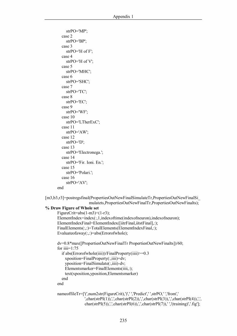
Appendix 1
235
strPO='MP'; case 2 strPO='BP'; case 3 strPO='H of F'; case 4 strPO='H of V'; case 5 strPO='MHC'; case 6 strPO='SHC'; case 7 strPO='TC'; case 8 strPO='EC'; case 9 strPO='WF'; case 10 strPO='LTherExC'; case 11 strPO='AW'; case 12 strPO='D'; case 13 strPO='Electronega.'; case 14 strPO='Fir. Ioni. En.'; case 15 strPO='Polari.'; case 16 strPO='AV'; end [m3,b3,r3]=postregsfinal(PropertiesOutNewFinalSimulateTr,PropertiesOutNewFinalSi_
mulatets,PropertiesOutNewFinalTr,PropertiesOutNewFinalts); % Draw Figure of Whole set FigureCrit=abs(1-m3)+(1-r3); ElementIndex=index(:,1,indexoftime(indexofneuron),indexofneuron); ElementIndexFinal=ElementIndex([iitrFinal,iitstFinal],:); FinalElements(:,:)=TotalElements(ElementIndexFinal,:); Evaluateofaway(:,:)=abs(Errorofwhole); dv=0.8*max([PropertiesOutNewFinalTr PropertiesOutNewFinalts])/60; for iiii=1:75 if abs(Errorofwhole(iiii))/FinalProperty(iiii)>=0.3 xposition=FinalProperty(:,iiii)+dv; yposition=FinalSimulate(:,iiii)-dv; Elementsmarker=FinalElements(iiii,:); text(xposition,yposition,Elementsmarker) end end nameoffileTr=['(',num2str(FigureCrit),')',' ','Predict',' ',strPO,' ','from','
',char(strPI(1)),',',char(strPI(2)),',',char(strPI(3)),',',char(strPI(4)),',',char(strPI(5)),',',char(strPI(6)),',',char(strPI(7)),' ','(training)','.fig'];
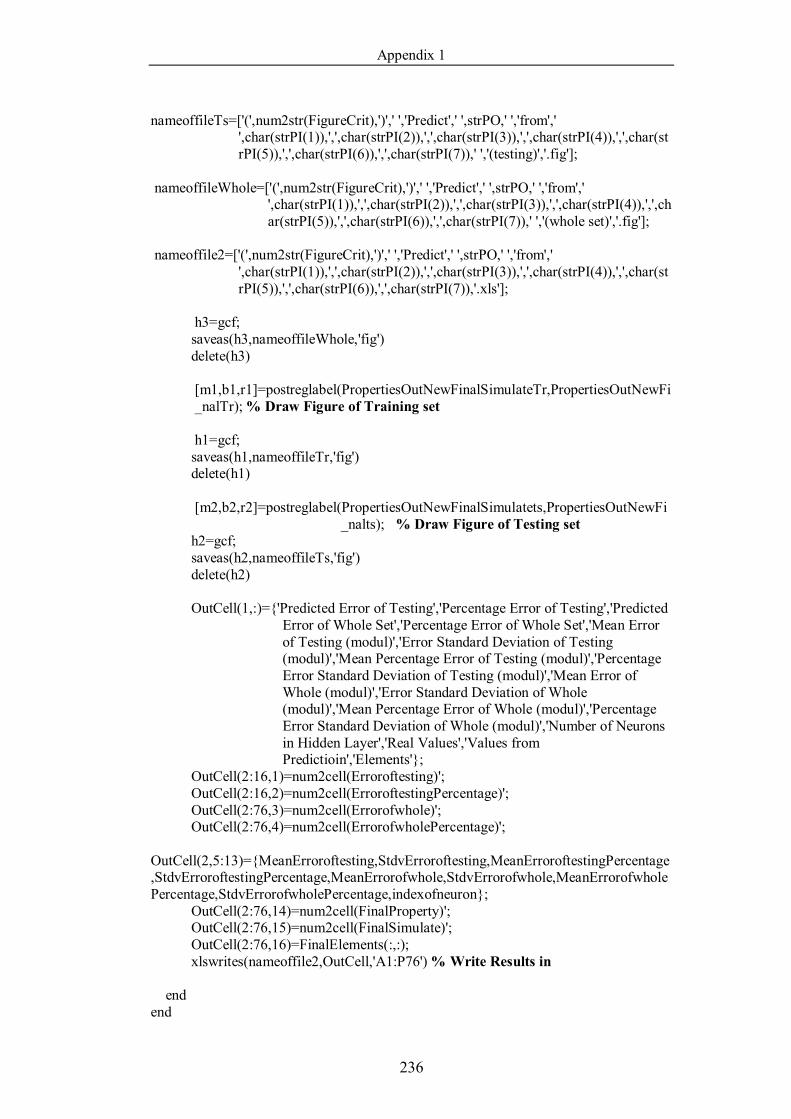
Appendix 1
236
nameoffileTs=['(',num2str(FigureCrit),')',' ','Predict',' ',strPO,' ','from','
',char(strPI(1)),',',char(strPI(2)),',',char(strPI(3)),',',char(strPI(4)),',',char(strPI(5)),',',char(strPI(6)),',',char(strPI(7)),' ','(testing)','.fig'];
nameoffileWhole=['(',num2str(FigureCrit),')',' ','Predict',' ',strPO,' ','from','
',char(strPI(1)),',',char(strPI(2)),',',char(strPI(3)),',',char(strPI(4)),',',char(strPI(5)),',',char(strPI(6)),',',char(strPI(7)),' ','(whole set)','.fig'];
nameoffile2=['(',num2str(FigureCrit),')',' ','Predict',' ',strPO,' ','from','
',char(strPI(1)),',',char(strPI(2)),',',char(strPI(3)),',',char(strPI(4)),',',char(strPI(5)),',',char(strPI(6)),',',char(strPI(7)),'.xls'];
h3=gcf;
saveas(h3,nameoffileWhole,'fig') delete(h3)
[m1,b1,r1]=postreglabel(PropertiesOutNewFinalSimulateTr,PropertiesOutNewFi _nalTr); % Draw Figure of Training set
h1=gcf;
saveas(h1,nameoffileTr,'fig') delete(h1)
[m2,b2,r2]=postreglabel(PropertiesOutNewFinalSimulatets,PropertiesOutNewFi _nalts); % Draw Figure of Testing set
h2=gcf; saveas(h2,nameoffileTs,'fig') delete(h2) OutCell(1,:)={'Predicted Error of Testing','Percentage Error of Testing','Predicted
Error of Whole Set','Percentage Error of Whole Set','Mean Error of Testing (modul)','Error Standard Deviation of Testing (modul)','Mean Percentage Error of Testing (modul)','Percentage Error Standard Deviation of Testing (modul)','Mean Error of Whole (modul)','Error Standard Deviation of Whole (modul)','Mean Percentage Error of Whole (modul)','Percentage Error Standard Deviation of Whole (modul)','Number of Neurons in Hidden Layer','Real Values','Values from Predictioin','Elements'};
OutCell(2:16,1)=num2cell(Erroroftesting)'; OutCell(2:16,2)=num2cell(ErroroftestingPercentage)'; OutCell(2:76,3)=num2cell(Errorofwhole)'; OutCell(2:76,4)=num2cell(ErrorofwholePercentage)'; OutCell(2,5:13)={MeanErroroftesting,StdvErroroftesting,MeanErroroftestingPercentage,StdvErroroftestingPercentage,MeanErrorofwhole,StdvErrorofwhole,MeanErrorofwholePercentage,StdvErrorofwholePercentage,indexofneuron}; OutCell(2:76,14)=num2cell(FinalProperty)'; OutCell(2:76,15)=num2cell(FinalSimulate)'; OutCell(2:76,16)=FinalElements(:,:); xlswrites(nameoffile2,OutCell,'A1:P76') % Write Results in end end
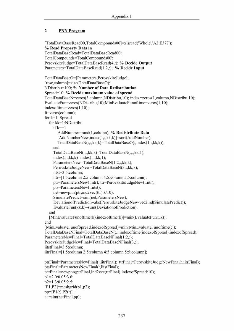
Appendix 1
237
2 PNN Program
[TotalDataBaseRead00,TotalCompounds00]=xlsread('Whole','A2:E377'); % Read Property Data in TotalDataBaseRead=TotalDataBaseRead00'; TotalCompounds=TotalCompounds00'; PerovskiteJudge=TotalDataBaseRead(4,:); % Decide Output Parameters=TotalDataBaseRead(1:2,:); % Decide Input TotalDataBaseO=[Parameters;PerovskiteJudge]; [row,column]=size(TotalDataBaseO); NDistribu=100; % Number of Data Redistribution Spread=10; % Decide maximum value of spread TotalDataBaseN=zeros(3,column,NDistribu,10); index=zeros(1,column,NDistribu,10); EvaluateFun=zeros(NDistribu,10);MinEvaluateFunoftime=zeros(1,10); indexoftime=zeros(1,10); ft=zeros(column); for k=1: Spread for kk=1:NDistribu if k==1 AddNumber=rand(1,column); % Redistribute Data [AddNumberNew,index(1,:,kk,k)]=sort(AddNumber); TotalDataBaseN(:,:,kk,k)=TotalDataBaseO(:,index(1,:,kk,k)); end TotalDataBaseN(:,:,kk,k)=TotalDataBaseN(:,:,kk,1); index(:,:,kk,k)=index(:,:,kk,1); ParametersNew=TotalDataBaseN(1:2,:,kk,k); PerovskiteJudgeNew=TotalDataBaseN(3,:,kk,k); iitst=3:5:column; iitr=[1:5:column 2:5:column 4:5:column 5:5:column]; ptr=ParametersNew(:,iitr); ttr=PerovskiteJudgeNew(:,iitr); pts=ParametersNew(:,iitst); net=newpnn(ptr,ind2vec(ttr),k/10); SimulatePredict=sim(net,ParametersNew); DeviationofPrediction=abs(PerovskiteJudgeNew-vec2ind(SimulatePredict)); EvaluateFun(kk,k)=sum(DeviationofPrediction); end [MinEvaluateFunoftime(k),indexoftime(k)]=min(EvaluateFun(:,k)); end [MinEvaluateFunofSpread,indexofSpread]=min(MinEvaluateFunoftime(:)); TotalDataBaseNFinal=TotalDataBaseN(:,:,indexoftime(indexofSpread),indexofSpread); ParametersNewFinal=TotalDataBaseNFinal(1:2,:); PerovskiteJudgeNewFinal=TotalDataBaseNFinal(3,:); iitstFinal=3:5:column; iitrFinal=[1:5:column 2:5:column 4:5:column 5:5:column]; ptrFinal=ParametersNewFinal(:,iitrFinal); ttrFinal=PerovskiteJudgeNewFinal(:,iitrFinal); ptsFinal=ParametersNewFinal(:,iitstFinal); netFinal=newpnn(ptrFinal,ind2vec(ttrFinal),indexofSpread/10); p1=2.0:0.05:3.6; p2=1.3:0.05:2.5; [P1,P2]=meshgrid(p1,p2); pp=[P1(:) P2(:)]'; aa=sim(netFinal,pp);

Appendix 1
238
aa=full(aa); m=mesh(P1,P2,reshape(aa(1,:),length(p2),length(p1))); set(m,'facecolor','yellow','linestyle','none'); % Non-perovskite hold on m=mesh(P1,P2,reshape(aa(2,:),length(p2),length(p1))); % Perovskite set(m,'facecolor','green','linestyle','none'); plot3(TotalDataBaseRead(1,1:144),TotalDataBaseRead(2,1:144),ones(1,144)+0.1,'x','ma
rkersize',7) plot3(TotalDataBaseRead(1,145:376),TotalDataBaseRead(2,145:376),ones(1,232)+0.1,'
diamond','markersize',7) bb=sim(netFinal,TotalDataBaseRead(1:2,:)); bb=full(bb); for i=1:column ft(i)=isequal(vec2ind(bb(:,i)),TotalDataBaseRead(4,i)); if ft(i)==0 text(TotalDataBaseRead(1,i),TotalDataBaseRead(2,i)+0.01,1.1,TotalCompounds(1,i),'fontsize',8); end end axis([2.0 3.6 1.3 2.5]) hold off view(2) title('The Classification of Perovskites and Non-Perovskites') xlabel('A-O Bond Distance') ylabel('B-O Bond Distance')
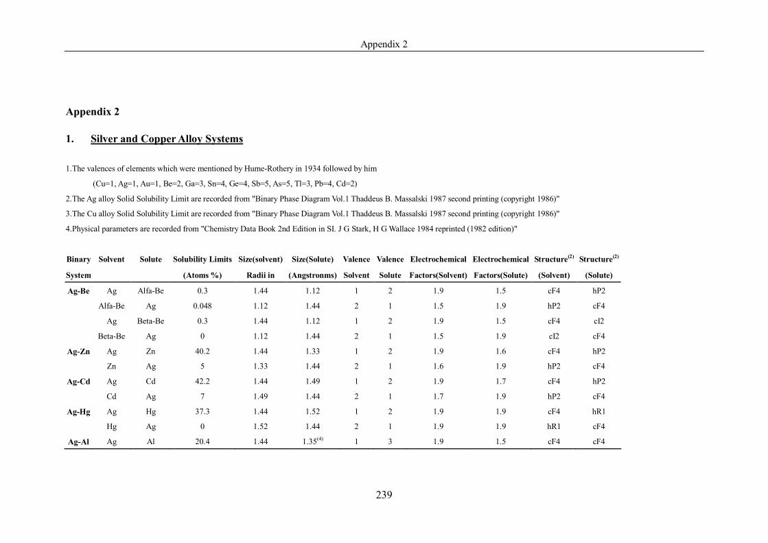
Appendix 2
239
Appendix 2
1. Silver and Copper Alloy Systems
1.The valences of elements which were mentioned by Hume-Rothery in 1934 followed by him
(Cu=1, Ag=1, Au=1, Be=2, Ga=3, Sn=4, Ge=4, Sb=5, As=5, Tl=3, Pb=4, Cd=2)
2.The Ag alloy Solid Solubility Limit are recorded from "Binary Phase Diagram Vol.1 Thaddeus B. Massalski 1987 second printing (copyright 1986)"
3.The Cu alloy Solid Solubility Limit are recorded from "Binary Phase Diagram Vol.1 Thaddeus B. Massalski 1987 second printing (copyright 1986)"
4.Physical parameters are recorded from "Chemistry Data Book 2nd Edition in SI. J G Stark, H G Wallace 1984 reprinted (1982 edition)"
Binary Solvent Solute Solubility Limits Size(solvent) Size(Solute) Valence Valence Electrochemical Electrochemical Structure(2) Structure(2)
System (Atoms %) Radii in (Angstronms) Solvent Solute Factors(Solvent) Factors(Solute) (Solvent) (Solute)
Ag-Be Ag Alfa-Be 0.3 1.44 1.12 1 2 1.9 1.5 cF4 hP2
Alfa-Be Ag 0.048 1.12 1.44 2 1 1.5 1.9 hP2 cF4
Ag Beta-Be 0.3 1.44 1.12 1 2 1.9 1.5 cF4 cI2
Beta-Be Ag 0 1.12 1.44 2 1 1.5 1.9 cI2 cF4
Ag-Zn Ag Zn 40.2 1.44 1.33 1 2 1.9 1.6 cF4 hP2
Zn Ag 5 1.33 1.44 2 1 1.6 1.9 hP2 cF4
Ag-Cd Ag Cd 42.2 1.44 1.49 1 2 1.9 1.7 cF4 hP2
Cd Ag 7 1.49 1.44 2 1 1.7 1.9 hP2 cF4
Ag-Hg Ag Hg 37.3 1.44 1.52 1 2 1.9 1.9 cF4 hR1
Hg Ag 0 1.52 1.44 2 1 1.9 1.9 hR1 cF4
Ag-Al Ag Al 20.4 1.44 1.35(4) 1 3 1.9 1.5 cF4 cF4
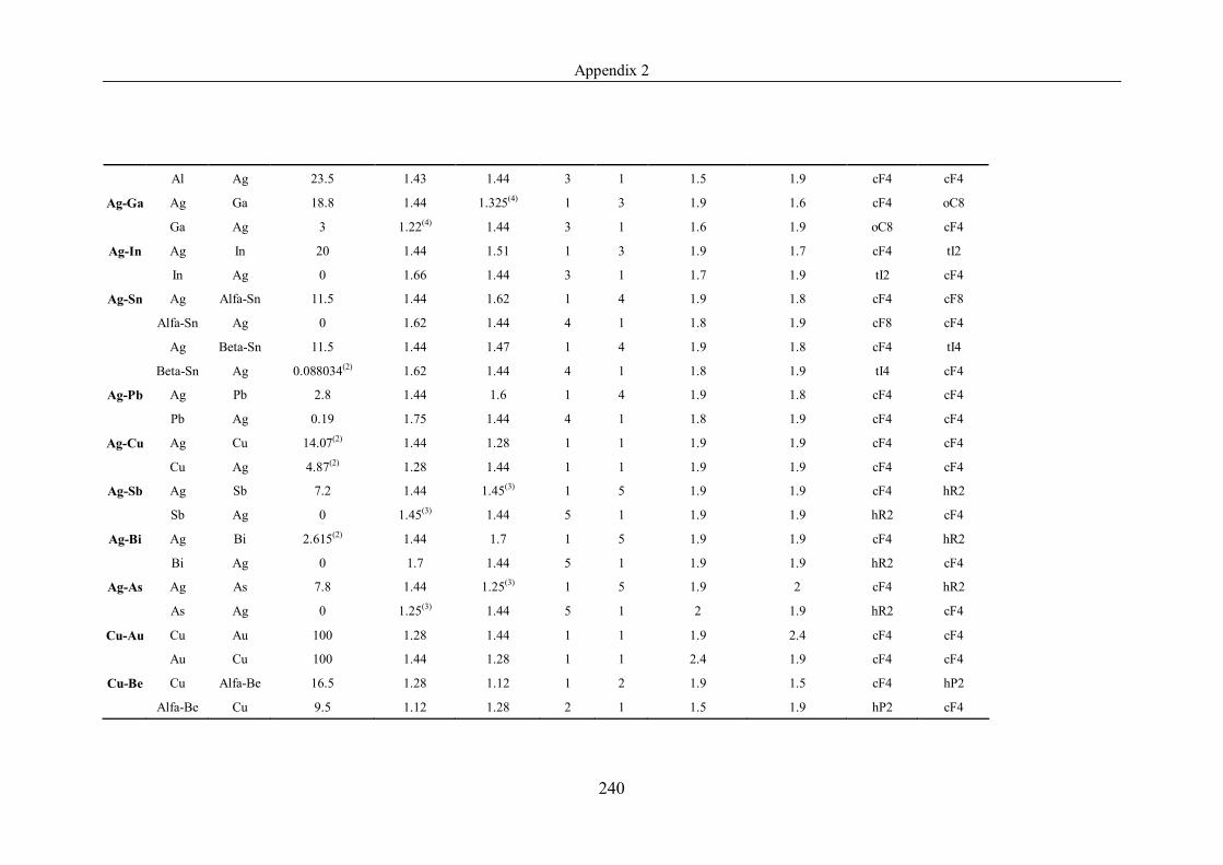
Appendix 2
240
Al Ag 23.5 1.43 1.44 3 1 1.5 1.9 cF4 cF4
Ag-Ga Ag Ga 18.8 1.44 1.325(4) 1 3 1.9 1.6 cF4 oC8
Ga Ag 3 1.22(4) 1.44 3 1 1.6 1.9 oC8 cF4
Ag-In Ag In 20 1.44 1.51 1 3 1.9 1.7 cF4 tI2
In Ag 0 1.66 1.44 3 1 1.7 1.9 tI2 cF4
Ag-Sn Ag Alfa-Sn 11.5 1.44 1.62 1 4 1.9 1.8 cF4 cF8
Alfa-Sn Ag 0 1.62 1.44 4 1 1.8 1.9 cF8 cF4
Ag Beta-Sn 11.5 1.44 1.47 1 4 1.9 1.8 cF4 tI4
Beta-Sn Ag 0.088034(2) 1.62 1.44 4 1 1.8 1.9 tI4 cF4
Ag-Pb Ag Pb 2.8 1.44 1.6 1 4 1.9 1.8 cF4 cF4
Pb Ag 0.19 1.75 1.44 4 1 1.8 1.9 cF4 cF4
Ag-Cu Ag Cu 14.07(2) 1.44 1.28 1 1 1.9 1.9 cF4 cF4
Cu Ag 4.87(2) 1.28 1.44 1 1 1.9 1.9 cF4 cF4
Ag-Sb Ag Sb 7.2 1.44 1.45(3) 1 5 1.9 1.9 cF4 hR2
Sb Ag 0 1.45(3) 1.44 5 1 1.9 1.9 hR2 cF4
Ag-Bi Ag Bi 2.615(2) 1.44 1.7 1 5 1.9 1.9 cF4 hR2
Bi Ag 0 1.7 1.44 5 1 1.9 1.9 hR2 cF4
Ag-As Ag As 7.8 1.44 1.25(3) 1 5 1.9 2 cF4 hR2
As Ag 0 1.25(3) 1.44 5 1 2 1.9 hR2 cF4
Cu-Au Cu Au 100 1.28 1.44 1 1 1.9 2.4 cF4 cF4
Au Cu 100 1.44 1.28 1 1 2.4 1.9 cF4 cF4
Cu-Be Cu Alfa-Be 16.5 1.28 1.12 1 2 1.9 1.5 cF4 hP2
Alfa-Be Cu 9.5 1.12 1.28 2 1 1.5 1.9 hP2 cF4
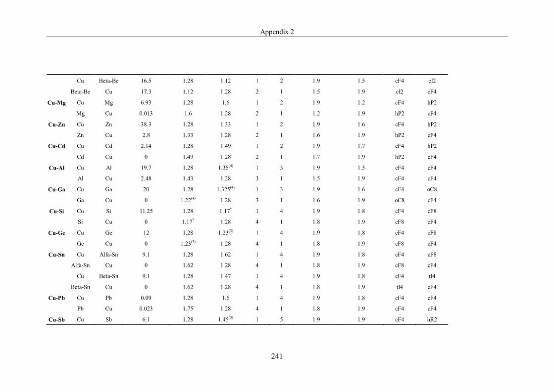
Appendix 2
241
Cu Beta-Be 16.5 1.28 1.12 1 2 1.9 1.5 cF4 cI2
Beta-Be Cu 17.3 1.12 1.28 2 1 1.5 1.9 cI2 cF4
Cu-Mg Cu Mg 6.93 1.28 1.6 1 2 1.9 1.2 cF4 hP2
Mg Cu 0.013 1.6 1.28 2 1 1.2 1.9 hP2 cF4
Cu-Zn Cu Zn 38.3 1.28 1.33 1 2 1.9 1.6 cF4 hP2
Zn Cu 2.8 1.33 1.28 2 1 1.6 1.9 hP2 cF4
Cu-Cd Cu Cd 2.14 1.28 1.49 1 2 1.9 1.7 cF4 hP2
Cd Cu 0 1.49 1.28 2 1 1.7 1.9 hP2 cF4
Cu-Al Cu Al 19.7 1.28 1.35(4) 1 3 1.9 1.5 cF4 cF4
Al Cu 2.48 1.43 1.28 3 1 1.5 1.9 cF4 cF4
Cu-Ga Cu Ga 20 1.28 1.325(4) 1 3 1.9 1.6 cF4 oC8
Ga Cu 0 1.22(4) 1.28 3 1 1.6 1.9 oC8 cF4
Cu-Si Cu Si 11.25 1.28 1.17* 1 4 1.9 1.8 cF4 cF8
Si Cu 0 1.17* 1.28 4 1 1.8 1.9 cF8 cF4
Cu-Ge Cu Ge 12 1.28 1.23(3) 1 4 1.9 1.8 cF4 cF8
Ge Cu 0 1.23(3) 1.28 4 1 1.8 1.9 cF8 cF4
Cu-Sn Cu Alfa-Sn 9.1 1.28 1.62 1 4 1.9 1.8 cF4 cF8
Alfa-Sn Cu 0 1.62 1.28 4 1 1.8 1.9 cF8 cF4
Cu Beta-Sn 9.1 1.28 1.47 1 4 1.9 1.8 cF4 tI4
Beta-Sn Cu 0 1.62 1.28 4 1 1.8 1.9 tI4 cF4
Cu-Pb Cu Pb 0.09 1.28 1.6 1 4 1.9 1.8 cF4 cF4
Pb Cu 0.023 1.75 1.28 4 1 1.8 1.9 cF4 cF4
Cu-Sb Cu Sb 6.1 1.28 1.45(3) 1 5 1.9 1.9 cF4 hR2
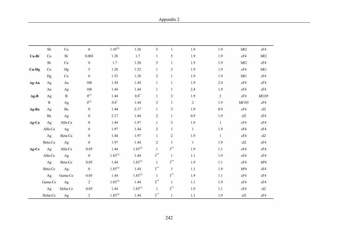
Appendix 2
242
Sb Cu 0 1.45(3) 1.28 5 1 1.9 1.9 hR2 cF4
Cu-Bi Cu Bi 0.003 1.28 1.7 1 5 1.9 1.9 cF4 hR2
Bi Cu 0 1.7 1.28 5 1 1.9 1.9 hR2 cF4
Cu-Hg Cu Hg 5 1.28 1.52 1 2 1.9 1.9 cF4 hR1
Hg Cu 0 1.52 1.28 2 1 1.9 1.9 hR1 cF4
Ag-Au Ag Au 100 1.44 1.44 1 1 1.9 2.4 cF4 cF4
Au Ag 100 1.44 1.44 1 1 2.4 1.9 cF4 cF4
Ag-B Ag B 0(1) 1.44 0.8* 1 3 1.9 2 cF4 hR105
B Ag 0(1) 0.8* 1.44 3 1 2 1.9 hR105 cF4
Ag-Ba Ag Ba 0 1.44 2.17 1 2 1.9 0.9 cF4 cI2
Ba Ag 0 2.17 1.44 2 1 0.9 1.9 cI2 cF4
Ag-Ca Ag Alfa-Ca 0 1.44 1.97 1 2 1.9 1 cF4 cF4
Alfa-Ca Ag 0 1.97 1.44 2 1 1 1.9 cF4 cF4
Ag Beta-Ca 0 1.44 1.97 1 2 1.9 1 cF4 cI2
Beta-Ca Ag 0 1.97 1.44 2 1 1 1.9 cI2 cF4
Ag-Ce Ag Alfa-Ce 0.05 1.44 1.83(3) 1 3** 1.9 1.1 cF4 cF4
Alfa-Ce Ag 0 1.83(3) 1.44 3** 1 1.1 1.9 cF4 cF4
Ag Beta-Ce 0.05 1.44 1.83(3) 1 3** 1.9 1.1 cF4 hP4
Beta-Ce Ag 0 1.83(3) 1.44 3** 1 1.1 1.9 hP4 cF4
Ag Gama-Ce 0.05 1.44 1.83(3) 1 3** 1.9 1.1 cF4 cF4
Gama-Ce Ag 2 1.83(3) 1.44 3** 1 1.1 1.9 cF4 cF4
Ag Delta-Ce 0.05 1.44 1.83(3) 1 3** 1.9 1.1 cF4 cI2
Delta-Ce Ag 2 1.83(3) 1.44 3** 1 1.1 1.9 cI2 cF4
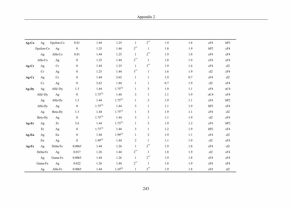
Appendix 2
243
Ag-Co Ag Epsilon-Co 0.81 1.44 1.25 1 2** 1.9 1.8 cF4 hP2
Epsilon-Co Ag 0 1.25 1.44 2** 1 1.8 1.9 hP2 cF4
Ag Alfa-Co 0.81 1.44 1.25 1 2** 1.9 1.8 cF4 cF4
Alfa-Co Ag 0 1.25 1.44 2** 1 1.8 1.9 cF4 cF4
Ag-Cr Ag Cr 0 1.44 1.25 1 3** 1.9 1.6 cF4 cI2
Cr Ag 0 1.25 1.44 3** 1 1.6 1.9 cI2 cF4
Ag-Cs Ag Cs 0 1.44 2.62 1 1 1.9 0.7 cF4 cI2
Cs Ag 0 2.62 1.44 1 1 0.7 1.9 cI2 cF4
Ag-Dy Ag Alfa'-Dy 1.3 1.44 1.75(3) 1 3 1.9 1.1 cF4 oC4
Alfa'-Dy Ag 0 1.75(3) 1.44 3 1 1.1 1.9 oC4 cF4
Ag Alfa-Dy 1.3 1.44 1.75(3) 1 3 1.9 1.1 cF4 hP2
Alfa-Dy Ag 0 1.75(3) 1.44 3 1 1.1 1.9 hP2 cF4
Ag Beta-Dy 1.3 1.44 1.75(3) 1 3 1.9 1.1 cF4 cI2
Bety-Dy Ag 0 1.75(3) 1.44 3 1 1.1 1.9 cI2 cF4
Ag-Er Ag Er 3.6 1.44 1.73(3) 1 3 1.9 1.2 cF4 hP2
Er Ag 0 1.73(3) 1.44 3 1 1.2 1.9 hP2 cF4
Ag-Eu Ag Eu 0 1.44 1.99(3) 1 2 1.9 1.1 cF4 cI2
Eu Ag 0 1.99(3) 1.44 2 1 1.1 1.9 cI2 cF4
Ag-Fe Ag Delta-Fe 0.0065 1.44 1.26 1 2** 1.9 1.8 cF4 cI2
Delta-Fe Ag 0.017 1.26 1.44 2** 1 1.8 1.9 cI2 cF4
Ag Gama-Fe 0.0065 1.44 1.26 1 2** 1.9 1.8 cF4 cF4
Gama-Fe Ag 0.022 1.26 1.44 2** 1 1.8 1.9 cF4 cF4
Ag Alfa-Fe 0.0065 1.44 1.24(4) 1 2** 1.9 1.8 cF4 cI2
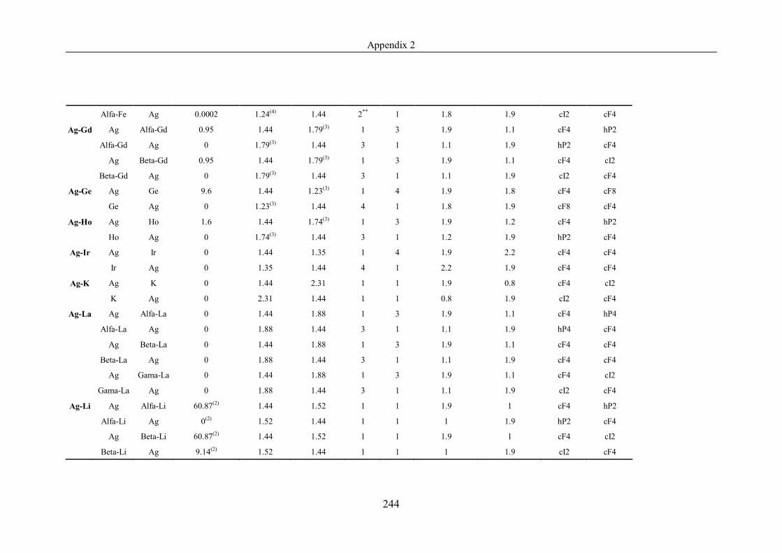
Appendix 2
244
Alfa-Fe Ag 0.0002 1.24(4) 1.44 2** 1 1.8 1.9 cI2 cF4
Ag-Gd Ag Alfa-Gd 0.95 1.44 1.79(3) 1 3 1.9 1.1 cF4 hP2
Alfa-Gd Ag 0 1.79(3) 1.44 3 1 1.1 1.9 hP2 cF4
Ag Beta-Gd 0.95 1.44 1.79(3) 1 3 1.9 1.1 cF4 cI2
Beta-Gd Ag 0 1.79(3) 1.44 3 1 1.1 1.9 cI2 cF4
Ag-Ge Ag Ge 9.6 1.44 1.23(3) 1 4 1.9 1.8 cF4 cF8
Ge Ag 0 1.23(3) 1.44 4 1 1.8 1.9 cF8 cF4
Ag-Ho Ag Ho 1.6 1.44 1.74(3) 1 3 1.9 1.2 cF4 hP2
Ho Ag 0 1.74(3) 1.44 3 1 1.2 1.9 hP2 cF4
Ag-Ir Ag Ir 0 1.44 1.35 1 4 1.9 2.2 cF4 cF4
Ir Ag 0 1.35 1.44 4 1 2.2 1.9 cF4 cF4
Ag-K Ag K 0 1.44 2.31 1 1 1.9 0.8 cF4 cI2
K Ag 0 2.31 1.44 1 1 0.8 1.9 cI2 cF4
Ag-La Ag Alfa-La 0 1.44 1.88 1 3 1.9 1.1 cF4 hP4
Alfa-La Ag 0 1.88 1.44 3 1 1.1 1.9 hP4 cF4
Ag Beta-La 0 1.44 1.88 1 3 1.9 1.1 cF4 cF4
Beta-La Ag 0 1.88 1.44 3 1 1.1 1.9 cF4 cF4
Ag Gama-La 0 1.44 1.88 1 3 1.9 1.1 cF4 cI2
Gama-La Ag 0 1.88 1.44 3 1 1.1 1.9 cI2 cF4
Ag-Li Ag Alfa-Li 60.87(2) 1.44 1.52 1 1 1.9 1 cF4 hP2
Alfa-Li Ag 0(2) 1.52 1.44 1 1 1 1.9 hP2 cF4
Ag Beta-Li 60.87(2) 1.44 1.52 1 1 1.9 1 cF4 cI2
Beta-Li Ag 9.14(2) 1.52 1.44 1 1 1 1.9 cI2 cF4
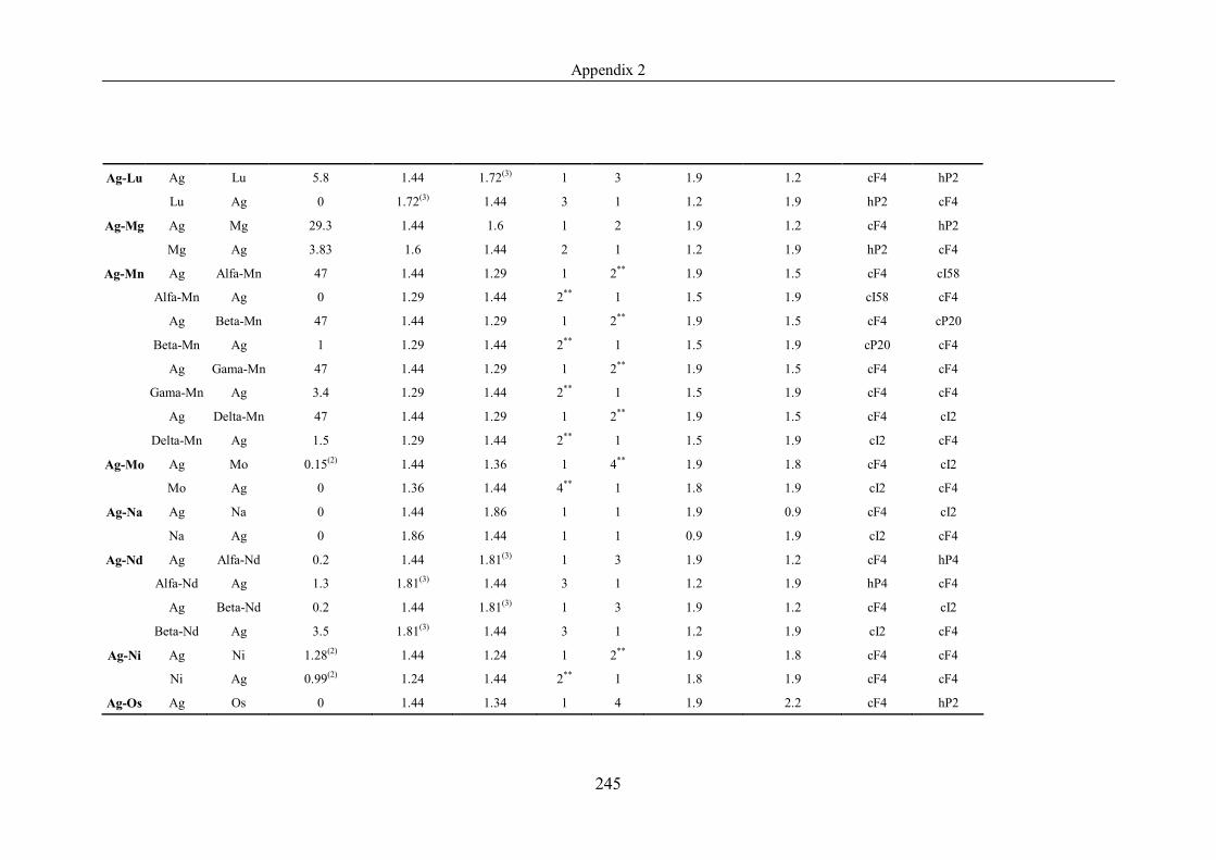
Appendix 2
245
Ag-Lu Ag Lu 5.8 1.44 1.72(3) 1 3 1.9 1.2 cF4 hP2
Lu Ag 0 1.72(3) 1.44 3 1 1.2 1.9 hP2 cF4
Ag-Mg Ag Mg 29.3 1.44 1.6 1 2 1.9 1.2 cF4 hP2
Mg Ag 3.83 1.6 1.44 2 1 1.2 1.9 hP2 cF4
Ag-Mn Ag Alfa-Mn 47 1.44 1.29 1 2** 1.9 1.5 cF4 cI58
Alfa-Mn Ag 0 1.29 1.44 2** 1 1.5 1.9 cI58 cF4
Ag Beta-Mn 47 1.44 1.29 1 2** 1.9 1.5 cF4 cP20
Beta-Mn Ag 1 1.29 1.44 2** 1 1.5 1.9 cP20 cF4
Ag Gama-Mn 47 1.44 1.29 1 2** 1.9 1.5 cF4 cF4
Gama-Mn Ag 3.4 1.29 1.44 2** 1 1.5 1.9 cF4 cF4
Ag Delta-Mn 47 1.44 1.29 1 2** 1.9 1.5 cF4 cI2
Delta-Mn Ag 1.5 1.29 1.44 2** 1 1.5 1.9 cI2 cF4
Ag-Mo Ag Mo 0.15(2) 1.44 1.36 1 4** 1.9 1.8 cF4 cI2
Mo Ag 0 1.36 1.44 4** 1 1.8 1.9 cI2 cF4
Ag-Na Ag Na 0 1.44 1.86 1 1 1.9 0.9 cF4 cI2
Na Ag 0 1.86 1.44 1 1 0.9 1.9 cI2 cF4
Ag-Nd Ag Alfa-Nd 0.2 1.44 1.81(3) 1 3 1.9 1.2 cF4 hP4
Alfa-Nd Ag 1.3 1.81(3) 1.44 3 1 1.2 1.9 hP4 cF4
Ag Beta-Nd 0.2 1.44 1.81(3) 1 3 1.9 1.2 cF4 cI2
Beta-Nd Ag 3.5 1.81(3) 1.44 3 1 1.2 1.9 cI2 cF4
Ag-Ni Ag Ni 1.28(2) 1.44 1.24 1 2** 1.9 1.8 cF4 cF4
Ni Ag 0.99(2) 1.24 1.44 2** 1 1.8 1.9 cF4 cF4
Ag-Os Ag Os 0 1.44 1.34 1 4 1.9 2.2 cF4 hP2
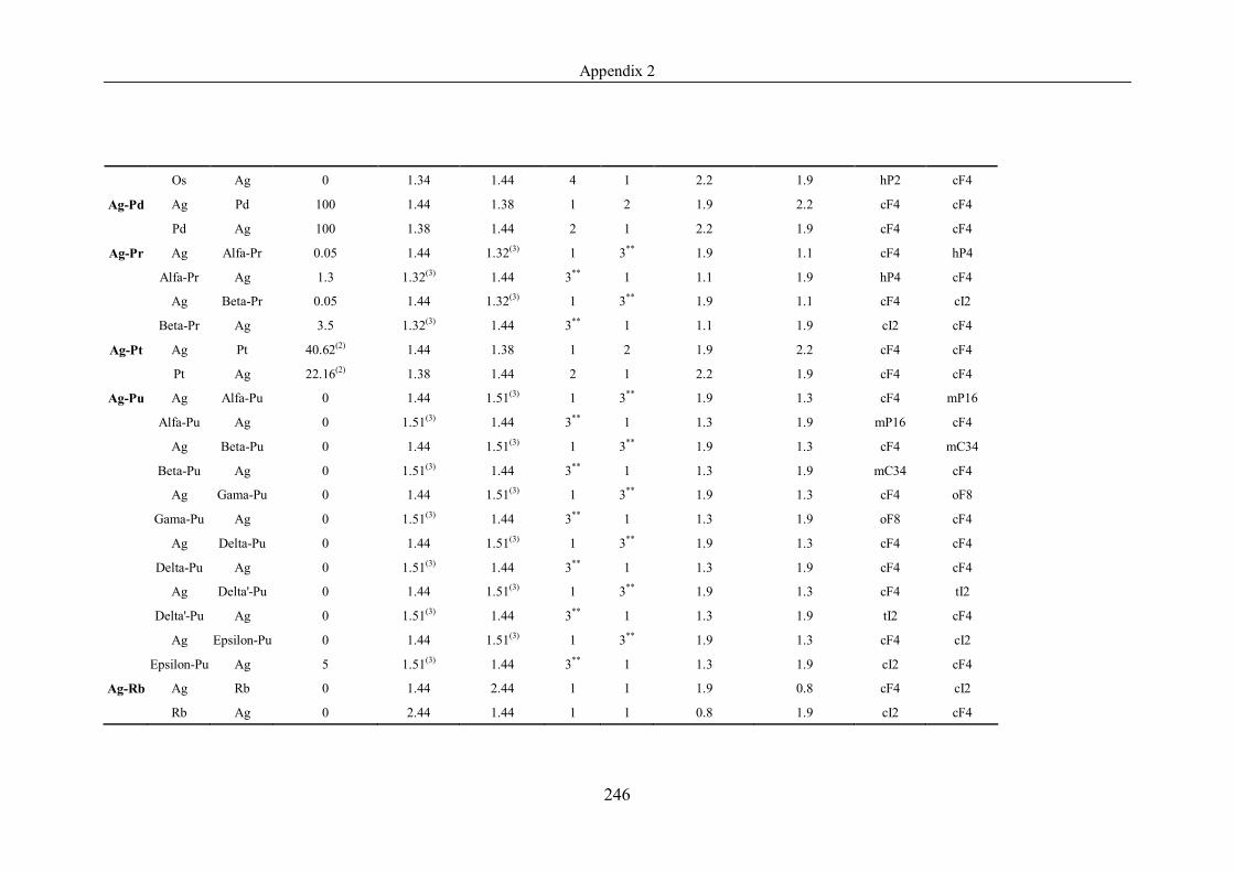
Appendix 2
246
Os Ag 0 1.34 1.44 4 1 2.2 1.9 hP2 cF4
Ag-Pd Ag Pd 100 1.44 1.38 1 2 1.9 2.2 cF4 cF4
Pd Ag 100 1.38 1.44 2 1 2.2 1.9 cF4 cF4
Ag-Pr Ag Alfa-Pr 0.05 1.44 1.32(3) 1 3** 1.9 1.1 cF4 hP4
Alfa-Pr Ag 1.3 1.32(3) 1.44 3** 1 1.1 1.9 hP4 cF4
Ag Beta-Pr 0.05 1.44 1.32(3) 1 3** 1.9 1.1 cF4 cI2
Beta-Pr Ag 3.5 1.32(3) 1.44 3** 1 1.1 1.9 cI2 cF4
Ag-Pt Ag Pt 40.62(2) 1.44 1.38 1 2 1.9 2.2 cF4 cF4
Pt Ag 22.16(2) 1.38 1.44 2 1 2.2 1.9 cF4 cF4
Ag-Pu Ag Alfa-Pu 0 1.44 1.51(3) 1 3** 1.9 1.3 cF4 mP16
Alfa-Pu Ag 0 1.51(3) 1.44 3** 1 1.3 1.9 mP16 cF4
Ag Beta-Pu 0 1.44 1.51(3) 1 3** 1.9 1.3 cF4 mC34
Beta-Pu Ag 0 1.51(3) 1.44 3** 1 1.3 1.9 mC34 cF4
Ag Gama-Pu 0 1.44 1.51(3) 1 3** 1.9 1.3 cF4 oF8
Gama-Pu Ag 0 1.51(3) 1.44 3** 1 1.3 1.9 oF8 cF4
Ag Delta-Pu 0 1.44 1.51(3) 1 3** 1.9 1.3 cF4 cF4
Delta-Pu Ag 0 1.51(3) 1.44 3** 1 1.3 1.9 cF4 cF4
Ag Delta'-Pu 0 1.44 1.51(3) 1 3** 1.9 1.3 cF4 tI2
Delta'-Pu Ag 0 1.51(3) 1.44 3** 1 1.3 1.9 tI2 cF4
Ag Epsilon-Pu 0 1.44 1.51(3) 1 3** 1.9 1.3 cF4 cI2
Epsilon-Pu Ag 5 1.51(3) 1.44 3** 1 1.3 1.9 cI2 cF4
Ag-Rb Ag Rb 0 1.44 2.44 1 1 1.9 0.8 cF4 cI2
Rb Ag 0 2.44 1.44 1 1 0.8 1.9 cI2 cF4
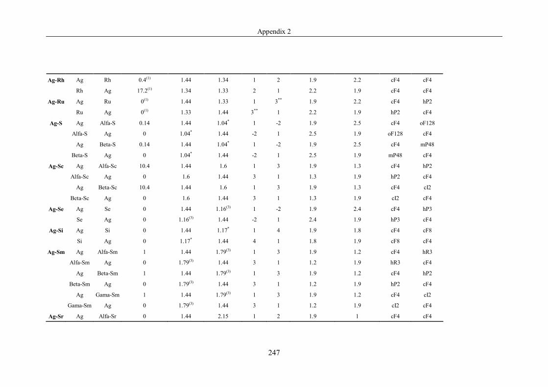
Appendix 2
247
Ag-Rh Ag Rh 0.4(1) 1.44 1.34 1 2 1.9 2.2 cF4 cF4
Rh Ag 17.2(1) 1.34 1.33 2 1 2.2 1.9 cF4 cF4
Ag-Ru Ag Ru 0(1) 1.44 1.33 1 3** 1.9 2.2 cF4 hP2
Ru Ag 0(1) 1.33 1.44 3** 1 2.2 1.9 hP2 cF4
Ag-S Ag Alfa-S 0.14 1.44 1.04* 1 -2 1.9 2.5 cF4 oF128
Alfa-S Ag 0 1.04* 1.44 -2 1 2.5 1.9 oF128 cF4
Ag Beta-S 0.14 1.44 1.04* 1 -2 1.9 2.5 cF4 mP48
Beta-S Ag 0 1.04* 1.44 -2 1 2.5 1.9 mP48 cF4
Ag-Sc Ag Alfa-Sc 10.4 1.44 1.6 1 3 1.9 1.3 cF4 hP2
Alfa-Sc Ag 0 1.6 1.44 3 1 1.3 1.9 hP2 cF4
Ag Beta-Sc 10.4 1.44 1.6 1 3 1.9 1.3 cF4 cI2
Beta-Sc Ag 0 1.6 1.44 3 1 1.3 1.9 cI2 cF4
Ag-Se Ag Se 0 1.44 1.16(3) 1 -2 1.9 2.4 cF4 hP3
Se Ag 0 1.16(3) 1.44 -2 1 2.4 1.9 hP3 cF4
Ag-Si Ag Si 0 1.44 1.17* 1 4 1.9 1.8 cF4 cF8
Si Ag 0 1.17* 1.44 4 1 1.8 1.9 cF8 cF4
Ag-Sm Ag Alfa-Sm 1 1.44 1.79(3) 1 3 1.9 1.2 cF4 hR3
Alfa-Sm Ag 0 1.79(3) 1.44 3 1 1.2 1.9 hR3 cF4
Ag Beta-Sm 1 1.44 1.79(3) 1 3 1.9 1.2 cF4 hP2
Beta-Sm Ag 0 1.79(3) 1.44 3 1 1.2 1.9 hP2 cF4
Ag Gama-Sm 1 1.44 1.79(3) 1 3 1.9 1.2 cF4 cI2
Gama-Sm Ag 0 1.79(3) 1.44 3 1 1.2 1.9 cI2 cF4
Ag-Sr Ag Alfa-Sr 0 1.44 2.15 1 2 1.9 1 cF4 cF4
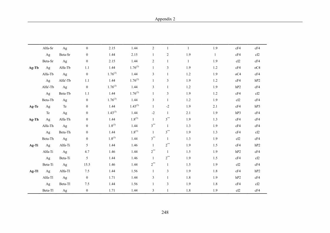
Appendix 2
248
Alfa-Sr Ag 0 2.15 1.44 2 1 1 1.9 cF4 cF4
Ag Beta-Sr 0 1.44 2.15 1 2 1.9 1 cF4 cI2
Beta-Sr Ag 0 2.15 1.44 2 1 1 1.9 cI2 cF4
Ag-Tb Ag Alfa-Tb 1.1 1.44 1.76(3) 1 3 1.9 1.2 cF4 oC4
Alfa-Tb Ag 0 1.76(3) 1.44 3 1 1.2 1.9 oC4 cF4
Ag Alfa'-Tb 1.1 1.44 1.76(3) 1 3 1.9 1.2 cF4 hP2
Alfa'-Tb Ag 0 1.76(3) 1.44 3 1 1.2 1.9 hP2 cF4
Ag Beta-Tb 1.1 1.44 1.76(3) 1 3 1.9 1.2 cF4 cI2
Beta-Tb Ag 0 1.76(3) 1.44 3 1 1.2 1.9 cI2 cF4
Ag-Te Ag Te 0 1.44 1.43(3) 1 -2 1.9 2.1 cF4 hP3
Te Ag 0 1.43(3) 1.44 -2 1 2.1 1.9 hP3 cF4
Ag-Th Ag Alfa-Th 0 1.44 1.8(3) 1 3** 1.9 1.3 cF4 cF4
Alfa-Th Ag 0 1.8(3) 1.44 3** 1 1.3 1.9 cF4 cF4
Ag Beta-Th 0 1.44 1.8(3) 1 3** 1.9 1.3 cF4 cI2
Beta-Th Ag 0 1.8(3) 1.44 3** 1 1.3 1.9 cI2 cF4
Ag-Ti Ag Alfa-Ti 5 1.44 1.46 1 2** 1.9 1.5 cF4 hP2
Alfa-Ti Ag 4.7 1.46 1.44 2** 1 1.5 1.9 hP2 cF4
Ag Beta-Ti 5 1.44 1.46 1 2** 1.9 1.5 cF4 cI2
Beta-Ti Ag 15.5 1.46 1.44 2** 1 1.5 1.9 cI2 cF4
Ag-Tl Ag Alfa-Tl 7.5 1.44 1.56 1 3 1.9 1.8 cF4 hP2
Alfa-Tl Ag 0 1.71 1.44 3 1 1.8 1.9 hP2 cF4
Ag Beta-Tl 7.5 1.44 1.56 1 3 1.9 1.8 cF4 cI2
Beta-Tl Ag 0 1.71 1.44 3 1 1.8 1.9 cI2 cF4

Appendix 2
249
Ag-Tm Ag Tm 4.57 1.44 1.72(3) 1 3 1.9 1.2 cF4 hP2
Tm Ag 0 1.72(3) 1.44 3 1 1.2 1.9 hP2 cF4
Ag-U Ag Alfa-U 2.3 1.44 1.39(3) 1 3** 1.9 1.7 cF4 oC4
Alfa-U Ag 0 1.39(3) 1.44 3** 1 1.7 1.9 oC4 cF4
Ag Beta-U 2.3 1.44 1.39(3) 1 3** 1.9 1.7 cF4 tP30
Beta-U Ag 0 1.39(3) 1.44 3** 1 1.7 1.9 tP30 cF4
Ag Gama-U 2.3 1.44 1.39(3) 1 3** 1.9 1.7 cF4 cI2
Gama-U Ag 0 1.39(3) 1.44 3** 1 1.7 1.9 cI2 cF4
Ag-V Ag V 0(1) 1.44 1.31 1 3** 1.9 1.6 cF4 cI2
V Ag 0(1) 1.31 1.44 3** 1 1.6 1.9 cI2 cF4
Ag-Y Ag Alfa-Y 1.31 1.44 1.8 1 3 1.9 1.2 cF4 hP2
Alfa-Y Ag 0 1.8 1.44 3 1 1.2 1.9 hP2 cF4
Ag Beta-Y 1.31 1.44 1.8 1 3 1.9 1.2 cF4 cI2
Beta-Y Ag 0 1.8 1.44 3 1 1.2 1.9 cI2 cF4
Ag-Yb Ag Alfa-Yb 1.92 1.44 1.94(3) 1 2 1.9 1.1 cF4 hP2
Alfa-Yb Ag 0 1.94(3) 1.44 2 1 1.1 1.9 hP2 cF4
Ag Beta-Yb 1.92 1.44 1.94(3) 1 2 1.9 1.1 cF4 cF4
Beta-Yb Ag 0 1.94(3) 1.44 2 1 1.1 1.9 cF4 cF4
Ag Gama-Yb 1.92 1.44 1.94(3) 1 2 1.9 1.1 cF4 cI2
Gama-Yb Ag 0 1.94(3) 1.44 2 1 1.1 1.9 cI2 cF4
Ag-Zr Ag Alfa-Zr 0.11 1.44 1.57 1 4 1.9 1.4 cF4 hP2
Alfa-Zr Ag 1.1 1.57 1.44 4 1 1.4 1.9 hP2 cF4
Ag Beta-Zr 0.11 1.44 1.57 1 4 1.9 1.4 cF4 cI2
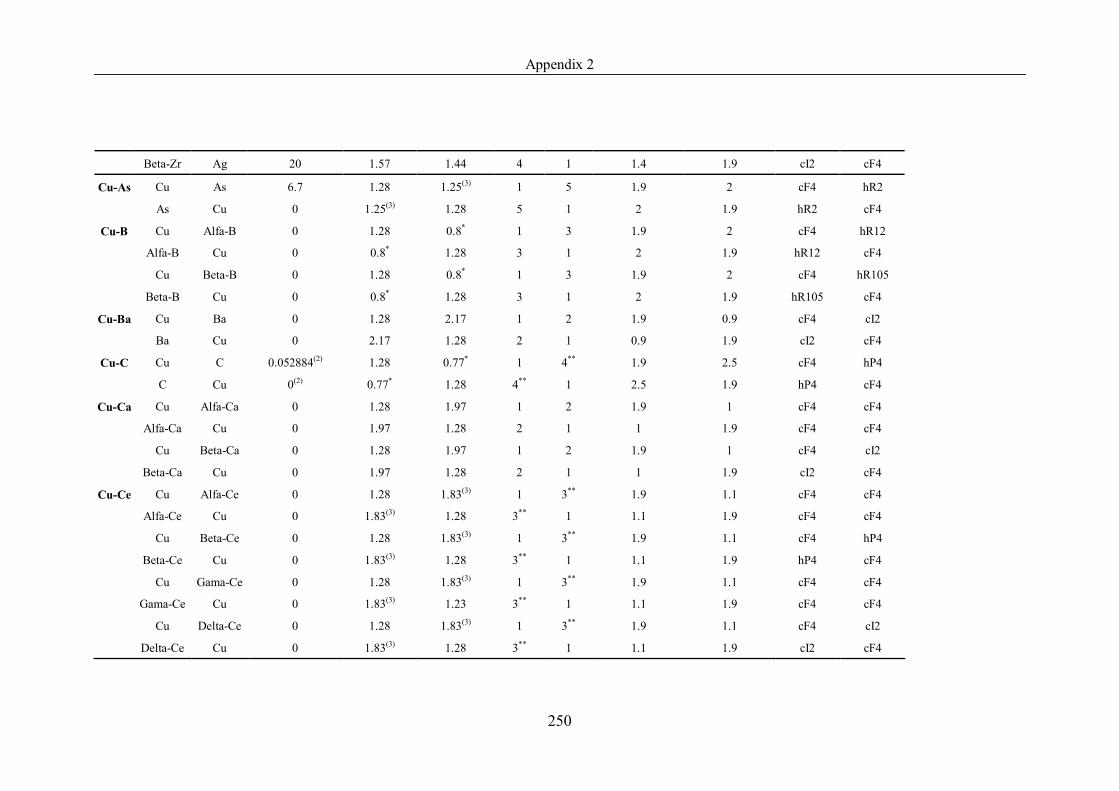
Appendix 2
250
Beta-Zr Ag 20 1.57 1.44 4 1 1.4 1.9 cI2 cF4
Cu-As Cu As 6.7 1.28 1.25(3) 1 5 1.9 2 cF4 hR2
As Cu 0 1.25(3) 1.28 5 1 2 1.9 hR2 cF4
Cu-B Cu Alfa-B 0 1.28 0.8* 1 3 1.9 2 cF4 hR12
Alfa-B Cu 0 0.8* 1.28 3 1 2 1.9 hR12 cF4
Cu Beta-B 0 1.28 0.8* 1 3 1.9 2 cF4 hR105
Beta-B Cu 0 0.8* 1.28 3 1 2 1.9 hR105 cF4
Cu-Ba Cu Ba 0 1.28 2.17 1 2 1.9 0.9 cF4 cI2
Ba Cu 0 2.17 1.28 2 1 0.9 1.9 cI2 cF4
Cu-C Cu C 0.052884(2) 1.28 0.77* 1 4** 1.9 2.5 cF4 hP4
C Cu 0(2) 0.77* 1.28 4** 1 2.5 1.9 hP4 cF4
Cu-Ca Cu Alfa-Ca 0 1.28 1.97 1 2 1.9 1 cF4 cF4
Alfa-Ca Cu 0 1.97 1.28 2 1 1 1.9 cF4 cF4
Cu Beta-Ca 0 1.28 1.97 1 2 1.9 1 cF4 cI2
Beta-Ca Cu 0 1.97 1.28 2 1 1 1.9 cI2 cF4
Cu-Ce Cu Alfa-Ce 0 1.28 1.83(3) 1 3** 1.9 1.1 cF4 cF4
Alfa-Ce Cu 0 1.83(3) 1.28 3** 1 1.1 1.9 cF4 cF4
Cu Beta-Ce 0 1.28 1.83(3) 1 3** 1.9 1.1 cF4 hP4
Beta-Ce Cu 0 1.83(3) 1.28 3** 1 1.1 1.9 hP4 cF4
Cu Gama-Ce 0 1.28 1.83(3) 1 3** 1.9 1.1 cF4 cF4
Gama-Ce Cu 0 1.83(3) 1.23 3** 1 1.1 1.9 cF4 cF4
Cu Delta-Ce 0 1.28 1.83(3) 1 3** 1.9 1.1 cF4 cI2
Delta-Ce Cu 0 1.83(3) 1.28 3** 1 1.1 1.9 cI2 cF4
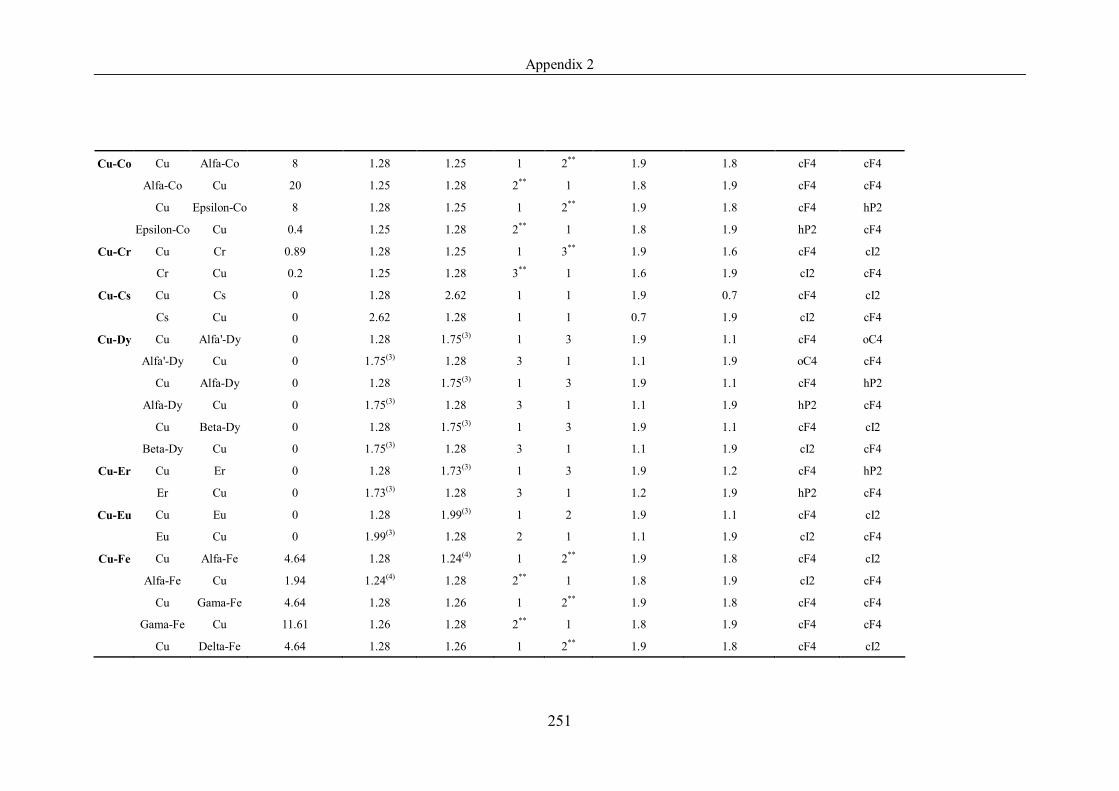
Appendix 2
251
Cu-Co Cu Alfa-Co 8 1.28 1.25 1 2** 1.9 1.8 cF4 cF4
Alfa-Co Cu 20 1.25 1.28 2** 1 1.8 1.9 cF4 cF4
Cu Epsilon-Co 8 1.28 1.25 1 2** 1.9 1.8 cF4 hP2
Epsilon-Co Cu 0.4 1.25 1.28 2** 1 1.8 1.9 hP2 cF4
Cu-Cr Cu Cr 0.89 1.28 1.25 1 3** 1.9 1.6 cF4 cI2
Cr Cu 0.2 1.25 1.28 3** 1 1.6 1.9 cI2 cF4
Cu-Cs Cu Cs 0 1.28 2.62 1 1 1.9 0.7 cF4 cI2
Cs Cu 0 2.62 1.28 1 1 0.7 1.9 cI2 cF4
Cu-Dy Cu Alfa'-Dy 0 1.28 1.75(3) 1 3 1.9 1.1 cF4 oC4
Alfa'-Dy Cu 0 1.75(3) 1.28 3 1 1.1 1.9 oC4 cF4
Cu Alfa-Dy 0 1.28 1.75(3) 1 3 1.9 1.1 cF4 hP2
Alfa-Dy Cu 0 1.75(3) 1.28 3 1 1.1 1.9 hP2 cF4
Cu Beta-Dy 0 1.28 1.75(3) 1 3 1.9 1.1 cF4 cI2
Beta-Dy Cu 0 1.75(3) 1.28 3 1 1.1 1.9 cI2 cF4
Cu-Er Cu Er 0 1.28 1.73(3) 1 3 1.9 1.2 cF4 hP2
Er Cu 0 1.73(3) 1.28 3 1 1.2 1.9 hP2 cF4
Cu-Eu Cu Eu 0 1.28 1.99(3) 1 2 1.9 1.1 cF4 cI2
Eu Cu 0 1.99(3) 1.28 2 1 1.1 1.9 cI2 cF4
Cu-Fe Cu Alfa-Fe 4.64 1.28 1.24(4) 1 2** 1.9 1.8 cF4 cI2
Alfa-Fe Cu 1.94 1.24(4) 1.28 2** 1 1.8 1.9 cI2 cF4
Cu Gama-Fe 4.64 1.28 1.26 1 2** 1.9 1.8 cF4 cF4
Gama-Fe Cu 11.61 1.26 1.28 2** 1 1.8 1.9 cF4 cF4
Cu Delta-Fe 4.64 1.28 1.26 1 2** 1.9 1.8 cF4 cI2
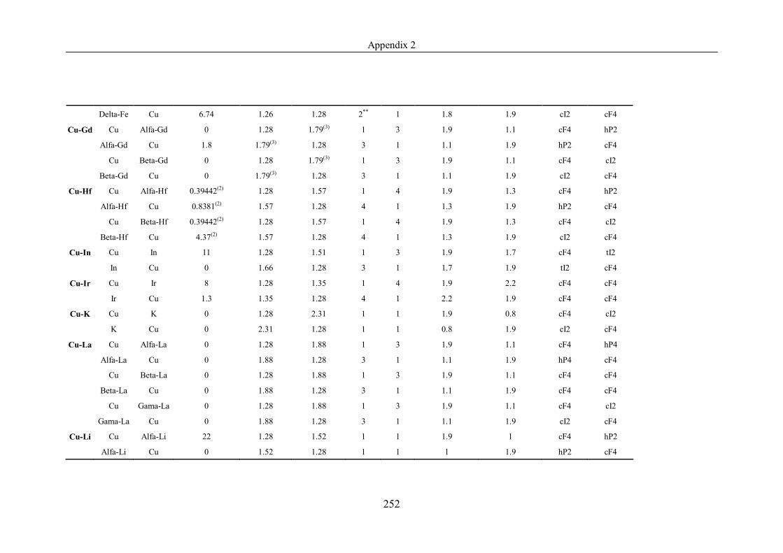
Appendix 2
252
Delta-Fe Cu 6.74 1.26 1.28 2** 1 1.8 1.9 cI2 cF4
Cu-Gd Cu Alfa-Gd 0 1.28 1.79(3) 1 3 1.9 1.1 cF4 hP2
Alfa-Gd Cu 1.8 1.79(3) 1.28 3 1 1.1 1.9 hP2 cF4
Cu Beta-Gd 0 1.28 1.79(3) 1 3 1.9 1.1 cF4 cI2
Beta-Gd Cu 0 1.79(3) 1.28 3 1 1.1 1.9 cI2 cF4
Cu-Hf Cu Alfa-Hf 0.39442(2) 1.28 1.57 1 4 1.9 1.3 cF4 hP2
Alfa-Hf Cu 0.8381(2) 1.57 1.28 4 1 1.3 1.9 hP2 cF4
Cu Beta-Hf 0.39442(2) 1.28 1.57 1 4 1.9 1.3 cF4 cI2
Beta-Hf Cu 4.37(2) 1.57 1.28 4 1 1.3 1.9 cI2 cF4
Cu-In Cu In 11 1.28 1.51 1 3 1.9 1.7 cF4 tI2
In Cu 0 1.66 1.28 3 1 1.7 1.9 tI2 cF4
Cu-Ir Cu Ir 8 1.28 1.35 1 4 1.9 2.2 cF4 cF4
Ir Cu 1.3 1.35 1.28 4 1 2.2 1.9 cF4 cF4
Cu-K Cu K 0 1.28 2.31 1 1 1.9 0.8 cF4 cI2
K Cu 0 2.31 1.28 1 1 0.8 1.9 cI2 cF4
Cu-La Cu Alfa-La 0 1.28 1.88 1 3 1.9 1.1 cF4 hP4
Alfa-La Cu 0 1.88 1.28 3 1 1.1 1.9 hP4 cF4
Cu Beta-La 0 1.28 1.88 1 3 1.9 1.1 cF4 cF4
Beta-La Cu 0 1.88 1.28 3 1 1.1 1.9 cF4 cF4
Cu Gama-La 0 1.28 1.88 1 3 1.9 1.1 cF4 cI2
Gama-La Cu 0 1.88 1.28 3 1 1.1 1.9 cI2 cF4
Cu-Li Cu Alfa-Li 22 1.28 1.52 1 1 1.9 1 cF4 hP2
Alfa-Li Cu 0 1.52 1.28 1 1 1 1.9 hP2 cF4
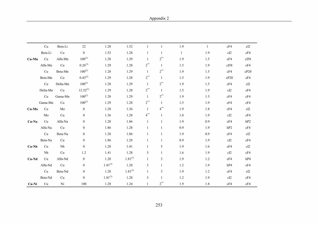
Appendix 2
253
Cu Beta-Li 22 1.28 1.52 1 1 1.9 1 cF4 cI2
Beta-Li Cu 0 1.52 1.28 1 1 1 1.9 cI2 cF4
Cu-Mn Cu Alfa-Mn 100(2) 1.28 1.29 1 2** 1.9 1.5 cF4 cI58
Alfa-Mn Cu 0.26(2) 1.29 1.28 2** 1 1.5 1.9 cI58 cF4
Cu Beta-Mn 100(2) 1.28 1.29 1 2** 1.9 1.5 cF4 cP20
Beta-Mn Cu 0.43(2) 1.29 1.28 2** 1 1.5 1.9 cP20 cF4
Cu Delta-Mn 100(2) 1.28 1.29 1 2** 1.9 1.5 cF4 cI2
Delta-Mn Cu 12.52(2) 1.29 1.28 2** 1 1.5 1.9 cI2 cF4
Cu Gama-Mn 100(2) 1.28 1.29 1 2** 1.9 1.5 cF4 cF4
Gama-Mn Cu 100(2) 1.29 1.28 2** 1 1.5 1.9 cF4 cF4
Cu-Mo Cu Mo 0 1.28 1.36 1 4** 1.9 1.8 cF4 cI2
Mo Cu 0 1.36 1.28 4** 1 1.8 1.9 cI2 cF4
Cu-Na Cu Alfa-Na 0 1.28 1.86 1 1 1.9 0.9 cF4 hP2
Alfa-Na Cu 0 1.86 1.28 1 1 0.9 1.9 hP2 cF4
Cu Beta-Na 0 1.28 1.86 1 1 1.9 0.9 cF4 cI2
Beta-Na Cu 0 1.86 1.28 1 1 0.9 1.9 cI2 cF4
Cu-Nb Cu Nb 0 1.28 1.41 1 5 1.9 1.6 cF4 cI2
Nb Cu 1.2 1.41 1.28 5 1 1.6 1.9 cI2 cF4
Cu-Nd Cu Alfa-Nd 0 1.28 1.81(3) 1 3 1.9 1.2 cF4 hP4
Alfa-Nd Cu 0 1.81(3) 1.28 3 1 1.2 1.9 hP4 cF4
Cu Beta-Nd 0 1.28 1.81(3) 1 3 1.9 1.2 cF4 cI2
Beta-Nd Cu 0 1.81(3) 1.28 3 1 1.2 1.9 cI2 cF4
Cu-Ni Cu Ni 100 1.28 1.24 1 2** 1.9 1.8 cF4 cF4
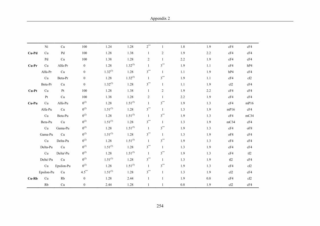
Appendix 2
254
Ni Cu 100 1.24 1.28 2** 1 1.8 1.9 cF4 cF4
Cu-Pd Cu Pd 100 1.28 1.38 1 2 1.9 2.2 cF4 cF4
Pd Cu 100 1.38 1.28 2 1 2.2 1.9 cF4 cF4
Cu-Pr Cu Alfa-Pr 0 1.28 1.32(3) 1 3** 1.9 1.1 cF4 hP4
Alfa-Pr Cu 0 1.32(3) 1.28 3** 1 1.1 1.9 hP4 cF4
Cu Beta-Pr 0 1.28 1.32(3) 1 3** 1.9 1.1 cF4 cI2
Beta-Pr Cu 0 1.32(3) 1.28 3** 1 1.1 1.9 cI2 cF4
Cu-Pt Cu Pt 100 1.28 1.38 1 2 1.9 2.2 cF4 cF4
Pt Cu 100 1.38 1.28 2 1 2.2 1.9 cF4 cF4
Cu-Pu Cu Alfa-Pu 0(2) 1.28 1.51(3) 1 3** 1.9 1.3 cF4 mP16
Alfa-Pu Cu 0(2) 1.51(3) 1.28 3** 1 1.3 1.9 mP16 cF4
Cu Beta-Pu 0(2) 1.28 1.51(3) 1 3** 1.9 1.3 cF4 mC34
Beta-Pu Cu 0(2) 1.51(3) 1.28 3** 1 1.3 1.9 mC34 cF4
Cu Gama-Pu 0(2) 1.28 1.51(3) 1 3** 1.9 1.3 cF4 oF8
Gama-Pu Cu 0(2) 1.51(3) 1.28 3** 1 1.3 1.9 oF8 cF4
Cu Delta-Pu 0(2) 1.28 1.51(3) 1 3** 1.9 1.3 cF4 cF4
Delta-Pu Cu 0(2) 1.51(3) 1.28 3** 1 1.3 1.9 cF4 cF4
Cu Delta'-Pu 0(2) 1.28 1.51(3) 1 3** 1.9 1.3 cF4 tI2
Delta'-Pu Cu 0(2) 1.51(3) 1.28 3** 1 1.3 1.9 tI2 cF4
Cu Epsilon-Pu 0(2) 1.28 1.51(3) 1 3** 1.9 1.3 cF4 cI2
Epsilon-Pu Cu 4.5** 1.51(3) 1.28 3** 1 1.3 1.9 cI2 cF4
Cu-Rb Cu Rb 0 1.28 2.44 1 1 1.9 0.8 cF4 cI2
Rb Cu 0 2.44 1.28 1 1 0.8 1.9 cI2 cF4
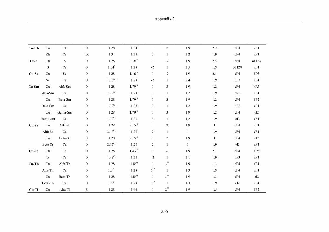
Appendix 2
255
Cu-Rh Cu Rh 100 1.28 1.34 1 2 1.9 2.2 cF4 cF4
Rh Cu 100 1.34 1.28 2 1 2.2 1.9 cF4 cF4
Cu-S Cu S 0 1.28 1.04* 1 -2 1.9 2.5 cF4 oF128
S Cu 0 1.04* 1.28 -2 1 2.5 1.9 oF128 cF4
Cu-Se Cu Se 0 1.28 1.16(3) 1 -2 1.9 2.4 cF4 hP3
Se Cu 0 1.16(3) 1.28 -2 1 2.4 1.9 hP3 cF4
Cu-Sm Cu Alfa-Sm 0 1.28 1.79(3) 1 3 1.9 1.2 cF4 hR3
Alfa-Sm Cu 0 1.79(3) 1.28 3 1 1.2 1.9 hR3 cF4
Cu Beta-Sm 0 1.28 1.79(3) 1 3 1.9 1.2 cF4 hP2
Beta-Sm Cu 0 1.79(3) 1.28 3 1 1.2 1.9 hP2 cF4
Cu Gama-Sm 0 1.28 1.79(3) 1 3 1.9 1.2 cF4 cI2
Gama-Sm Cu 0 1.79(3) 1.28 3 1 1.2 1.9 cI2 cF4
Cu-Sr Cu Alfa-Sr 0 1.28 2.15(3) 1 2 1.9 1 cF4 cF4
Alfa-Sr Cu 0 2.15(3) 1.28 2 1 1 1.9 cF4 cF4
Cu Beta-Sr 0 1.28 2.15(3) 1 2 1.9 1 cF4 cI2
Beta-Sr Cu 0 2.15(3) 1.28 2 1 1 1.9 cI2 cF4
Cu-Te Cu Te 0 1.28 1.43(3) 1 -2 1.9 2.1 cF4 hP3
Te Cu 0 1.43(3) 1.28 -2 1 2.1 1.9 hP3 cF4
Cu-Th Cu Alfa-Th 0 1.28 1.8(3) 1 3** 1.9 1.3 cF4 cF4
Alfa-Th Cu 0 1.8(3) 1.28 3** 1 1.3 1.9 cF4 cF4
Cu Beta-Th 0 1.28 1.8(3) 1 3** 1.9 1.3 cF4 cI2
Beta-Th Cu 0 1.8(3) 1.28 3** 1 1.3 1.9 cI2 cF4
Cu-Ti Cu Alfa-Ti 8 1.28 1.46 1 2** 1.9 1.5 cF4 hP2
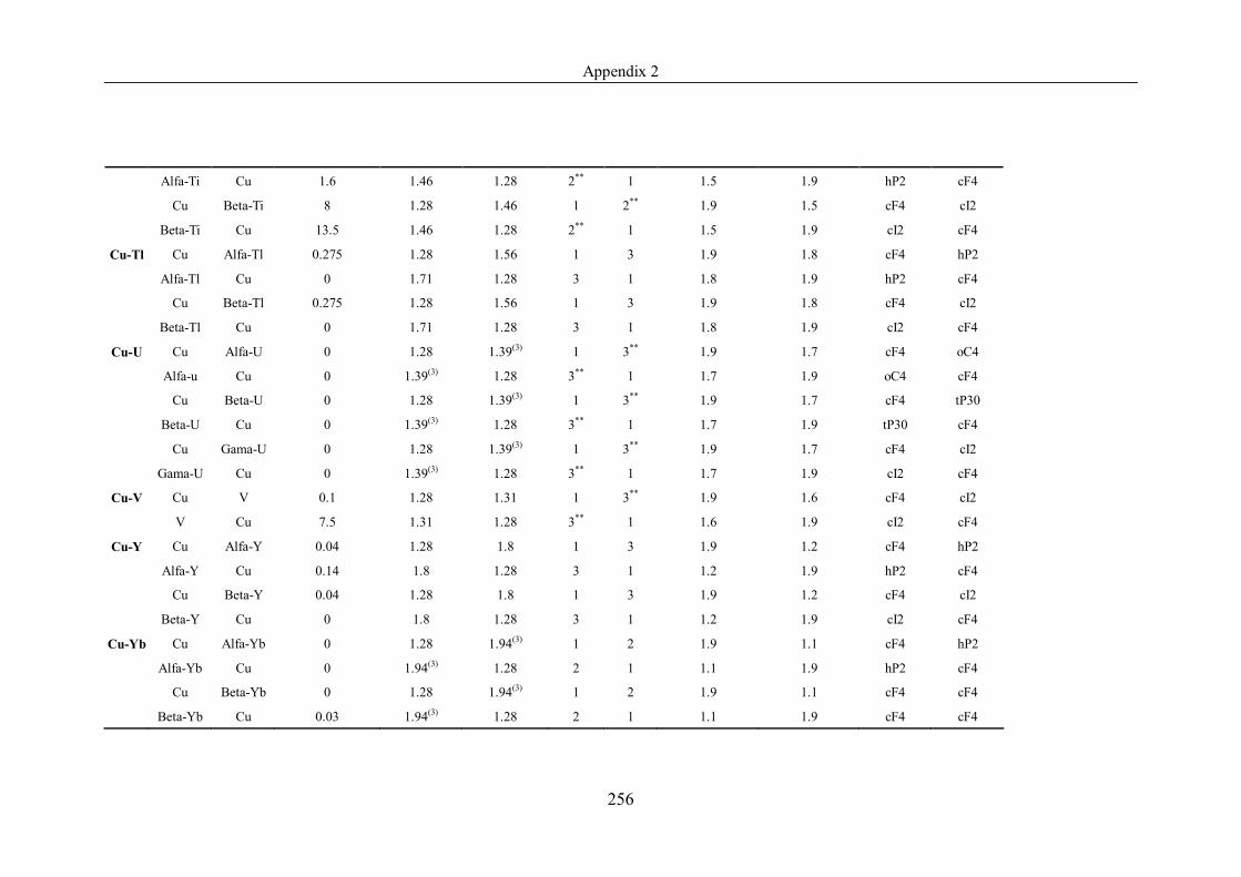
Appendix 2
256
Alfa-Ti Cu 1.6 1.46 1.28 2** 1 1.5 1.9 hP2 cF4
Cu Beta-Ti 8 1.28 1.46 1 2** 1.9 1.5 cF4 cI2
Beta-Ti Cu 13.5 1.46 1.28 2** 1 1.5 1.9 cI2 cF4
Cu-Tl Cu Alfa-Tl 0.275 1.28 1.56 1 3 1.9 1.8 cF4 hP2
Alfa-Tl Cu 0 1.71 1.28 3 1 1.8 1.9 hP2 cF4
Cu Beta-Tl 0.275 1.28 1.56 1 3 1.9 1.8 cF4 cI2
Beta-Tl Cu 0 1.71 1.28 3 1 1.8 1.9 cI2 cF4
Cu-U Cu Alfa-U 0 1.28 1.39(3) 1 3** 1.9 1.7 cF4 oC4
Alfa-u Cu 0 1.39(3) 1.28 3** 1 1.7 1.9 oC4 cF4
Cu Beta-U 0 1.28 1.39(3) 1 3** 1.9 1.7 cF4 tP30
Beta-U Cu 0 1.39(3) 1.28 3** 1 1.7 1.9 tP30 cF4
Cu Gama-U 0 1.28 1.39(3) 1 3** 1.9 1.7 cF4 cI2
Gama-U Cu 0 1.39(3) 1.28 3** 1 1.7 1.9 cI2 cF4
Cu-V Cu V 0.1 1.28 1.31 1 3** 1.9 1.6 cF4 cI2
V Cu 7.5 1.31 1.28 3** 1 1.6 1.9 cI2 cF4
Cu-Y Cu Alfa-Y 0.04 1.28 1.8 1 3 1.9 1.2 cF4 hP2
Alfa-Y Cu 0.14 1.8 1.28 3 1 1.2 1.9 hP2 cF4
Cu Beta-Y 0.04 1.28 1.8 1 3 1.9 1.2 cF4 cI2
Beta-Y Cu 0 1.8 1.28 3 1 1.2 1.9 cI2 cF4
Cu-Yb Cu Alfa-Yb 0 1.28 1.94(3) 1 2 1.9 1.1 cF4 hP2
Alfa-Yb Cu 0 1.94(3) 1.28 2 1 1.1 1.9 hP2 cF4
Cu Beta-Yb 0 1.28 1.94(3) 1 2 1.9 1.1 cF4 cF4
Beta-Yb Cu 0.03 1.94(3) 1.28 2 1 1.1 1.9 cF4 cF4
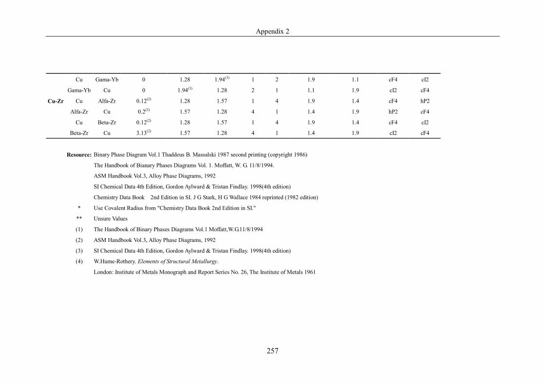
Appendix 2
257
Cu Gama-Yb 0 1.28 1.94(3) 1 2 1.9 1.1 cF4 cI2
Gama-Yb Cu 0 1.94(3) 1.28 2 1 1.1 1.9 cI2 cF4
Cu-Zr Cu Alfa-Zr 0.12(2) 1.28 1.57 1 4 1.9 1.4 cF4 hP2
Alfa-Zr Cu 0.2(2) 1.57 1.28 4 1 1.4 1.9 hP2 cF4
Cu Beta-Zr 0.12(2) 1.28 1.57 1 4 1.9 1.4 cF4 cI2
Beta-Zr Cu 3.13(2) 1.57 1.28 4 1 1.4 1.9 cI2 cF4
Resource: Binary Phase Diagram Vol.1 Thaddeus B. Massalski 1987 second printing (copyright 1986)
The Handbook of Bianary Phases Diagrams Vol. 1. Moffatt, W. G. 11/8/1994.
ASM Handbook Vol.3, Alloy Phase Diagrams, 1992
SI Chemical Data 4th Edition, Gordon Aylward & Tristan Findlay. 1998(4th edition)
Chemistry Data Book 2nd Edition in SI. J G Stark, H G Wallace 1984 reprinted (1982 edition)
* Use Covalent Radius from "Chemistry Data Book 2nd Edition in SI."
** Unsure Values
(1) The Handbook of Binary Phases Diagrams Vol.1 Moffatt,W.G.11/8/1994
(2) ASM Handbook Vol.3, Alloy Phase Diagrams, 1992
(3) SI Chemical Data 4th Edition, Gordon Aylward & Tristan Findlay. 1998(4th edition)
(4) W.Hume-Rothery. Elements of Structural Metallurgy.
London: Institute of Metals Monograph and Report Series No. 26, The Institute of Metals 1961
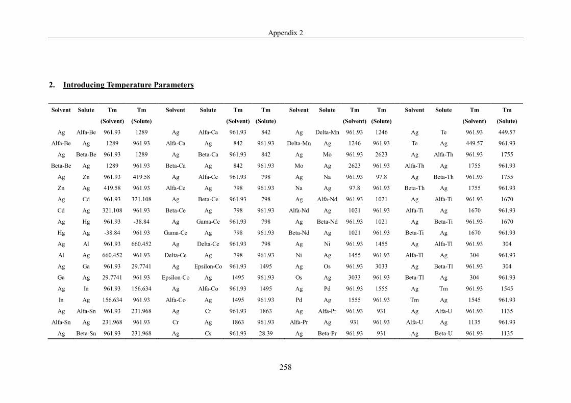
Appendix 2
258
2. Introducing Temperature Parameters Solvent Solute Tm Tm Solvent Solute Tm Tm Solvent Solute Tm Tm Solvent Solute Tm Tm
(Solvent) (Solute) (Solvent) (Solute) (Solvent) (Solute) (Solvent) (Solute)
Ag Alfa-Be 961.93 1289 Ag Alfa-Ca 961.93 842 Ag Delta-Mn 961.93 1246 Ag Te 961.93 449.57
Alfa-Be Ag 1289 961.93 Alfa-Ca Ag 842 961.93 Delta-Mn Ag 1246 961.93 Te Ag 449.57 961.93
Ag Beta-Be 961.93 1289 Ag Beta-Ca 961.93 842 Ag Mo 961.93 2623 Ag Alfa-Th 961.93 1755
Beta-Be Ag 1289 961.93 Beta-Ca Ag 842 961.93 Mo Ag 2623 961.93 Alfa-Th Ag 1755 961.93
Ag Zn 961.93 419.58 Ag Alfa-Ce 961.93 798 Ag Na 961.93 97.8 Ag Beta-Th 961.93 1755
Zn Ag 419.58 961.93 Alfa-Ce Ag 798 961.93 Na Ag 97.8 961.93 Beta-Th Ag 1755 961.93
Ag Cd 961.93 321.108 Ag Beta-Ce 961.93 798 Ag Alfa-Nd 961.93 1021 Ag Alfa-Ti 961.93 1670
Cd Ag 321.108 961.93 Beta-Ce Ag 798 961.93 Alfa-Nd Ag 1021 961.93 Alfa-Ti Ag 1670 961.93
Ag Hg 961.93 -38.84 Ag Gama-Ce 961.93 798 Ag Beta-Nd 961.93 1021 Ag Beta-Ti 961.93 1670
Hg Ag -38.84 961.93 Gama-Ce Ag 798 961.93 Beta-Nd Ag 1021 961.93 Beta-Ti Ag 1670 961.93
Ag Al 961.93 660.452 Ag Delta-Ce 961.93 798 Ag Ni 961.93 1455 Ag Alfa-Tl 961.93 304
Al Ag 660.452 961.93 Delta-Ce Ag 798 961.93 Ni Ag 1455 961.93 Alfa-Tl Ag 304 961.93
Ag Ga 961.93 29.7741 Ag Epsilon-Co 961.93 1495 Ag Os 961.93 3033 Ag Beta-Tl 961.93 304
Ga Ag 29.7741 961.93 Epsilon-Co Ag 1495 961.93 Os Ag 3033 961.93 Beta-Tl Ag 304 961.93
Ag In 961.93 156.634 Ag Alfa-Co 961.93 1495 Ag Pd 961.93 1555 Ag Tm 961.93 1545
In Ag 156.634 961.93 Alfa-Co Ag 1495 961.93 Pd Ag 1555 961.93 Tm Ag 1545 961.93
Ag Alfa-Sn 961.93 231.968 Ag Cr 961.93 1863 Ag Alfa-Pr 961.93 931 Ag Alfa-U 961.93 1135
Alfa-Sn Ag 231.968 961.93 Cr Ag 1863 961.93 Alfa-Pr Ag 931 961.93 Alfa-U Ag 1135 961.93
Ag Beta-Sn 961.93 231.968 Ag Cs 961.93 28.39 Ag Beta-Pr 961.93 931 Ag Beta-U 961.93 1135
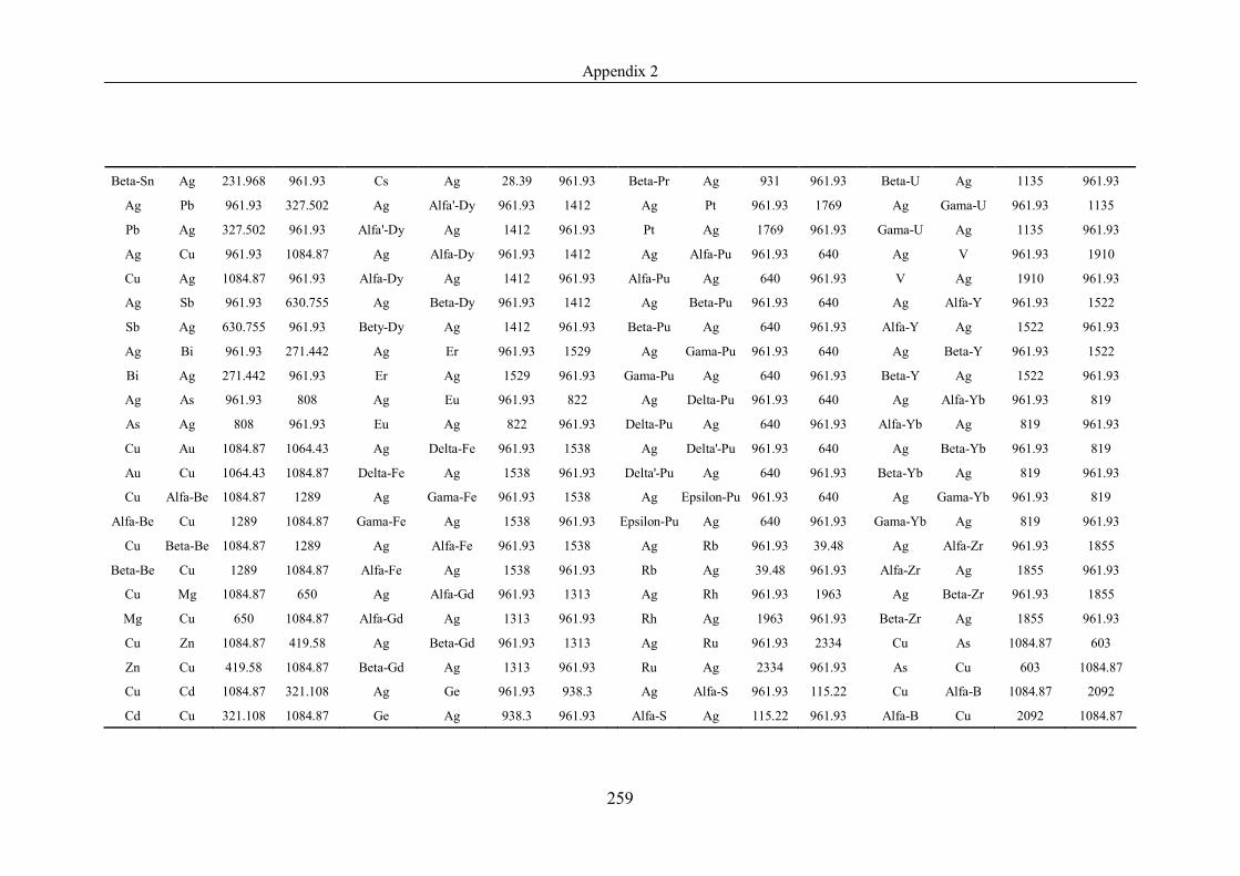
Appendix 2
259
Beta-Sn Ag 231.968 961.93 Cs Ag 28.39 961.93 Beta-Pr Ag 931 961.93 Beta-U Ag 1135 961.93
Ag Pb 961.93 327.502 Ag Alfa'-Dy 961.93 1412 Ag Pt 961.93 1769 Ag Gama-U 961.93 1135
Pb Ag 327.502 961.93 Alfa'-Dy Ag 1412 961.93 Pt Ag 1769 961.93 Gama-U Ag 1135 961.93
Ag Cu 961.93 1084.87 Ag Alfa-Dy 961.93 1412 Ag Alfa-Pu 961.93 640 Ag V 961.93 1910
Cu Ag 1084.87 961.93 Alfa-Dy Ag 1412 961.93 Alfa-Pu Ag 640 961.93 V Ag 1910 961.93
Ag Sb 961.93 630.755 Ag Beta-Dy 961.93 1412 Ag Beta-Pu 961.93 640 Ag Alfa-Y 961.93 1522
Sb Ag 630.755 961.93 Bety-Dy Ag 1412 961.93 Beta-Pu Ag 640 961.93 Alfa-Y Ag 1522 961.93
Ag Bi 961.93 271.442 Ag Er 961.93 1529 Ag Gama-Pu 961.93 640 Ag Beta-Y 961.93 1522
Bi Ag 271.442 961.93 Er Ag 1529 961.93 Gama-Pu Ag 640 961.93 Beta-Y Ag 1522 961.93
Ag As 961.93 808 Ag Eu 961.93 822 Ag Delta-Pu 961.93 640 Ag Alfa-Yb 961.93 819
As Ag 808 961.93 Eu Ag 822 961.93 Delta-Pu Ag 640 961.93 Alfa-Yb Ag 819 961.93
Cu Au 1084.87 1064.43 Ag Delta-Fe 961.93 1538 Ag Delta'-Pu 961.93 640 Ag Beta-Yb 961.93 819
Au Cu 1064.43 1084.87 Delta-Fe Ag 1538 961.93 Delta'-Pu Ag 640 961.93 Beta-Yb Ag 819 961.93
Cu Alfa-Be 1084.87 1289 Ag Gama-Fe 961.93 1538 Ag Epsilon-Pu 961.93 640 Ag Gama-Yb 961.93 819
Alfa-Be Cu 1289 1084.87 Gama-Fe Ag 1538 961.93 Epsilon-Pu Ag 640 961.93 Gama-Yb Ag 819 961.93
Cu Beta-Be 1084.87 1289 Ag Alfa-Fe 961.93 1538 Ag Rb 961.93 39.48 Ag Alfa-Zr 961.93 1855
Beta-Be Cu 1289 1084.87 Alfa-Fe Ag 1538 961.93 Rb Ag 39.48 961.93 Alfa-Zr Ag 1855 961.93
Cu Mg 1084.87 650 Ag Alfa-Gd 961.93 1313 Ag Rh 961.93 1963 Ag Beta-Zr 961.93 1855
Mg Cu 650 1084.87 Alfa-Gd Ag 1313 961.93 Rh Ag 1963 961.93 Beta-Zr Ag 1855 961.93
Cu Zn 1084.87 419.58 Ag Beta-Gd 961.93 1313 Ag Ru 961.93 2334 Cu As 1084.87 603
Zn Cu 419.58 1084.87 Beta-Gd Ag 1313 961.93 Ru Ag 2334 961.93 As Cu 603 1084.87
Cu Cd 1084.87 321.108 Ag Ge 961.93 938.3 Ag Alfa-S 961.93 115.22 Cu Alfa-B 1084.87 2092
Cd Cu 321.108 1084.87 Ge Ag 938.3 961.93 Alfa-S Ag 115.22 961.93 Alfa-B Cu 2092 1084.87
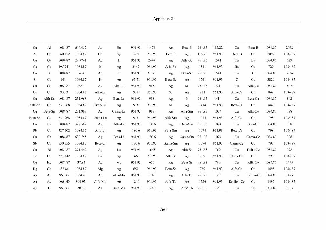
Appendix 2
260
Cu Al 1084.87 660.452 Ag Ho 961.93 1474 Ag Beta-S 961.93 115.22 Cu Beta-B 1084.87 2092
Al Cu 660.452 1084.87 Ho Ag 1474 961.93 Beta-S Ag 115.22 961.93 Beta-B Cu 2092 1084.87
Cu Ga 1084.87 29.7741 Ag Ir 961.93 2447 Ag Alfa-Sc 961.93 1541 Cu Ba 1084.87 729
Ga Cu 29.7741 1084.87 Ir Ag 2447 961.93 Alfa-Sc Ag 1541 961.93 Ba Cu 729 1084.87
Cu Si 1084.87 1414 Ag K 961.93 63.71 Ag Beta-Sc 961.93 1541 Cu C 1084.87 3826
Si Cu 1414 1084.87 K Ag 63.71 961.93 Beta-Sc Ag 1541 961.93 C Cu 3826 1084.87
Cu Ge 1084.87 938.3 Ag Alfa-La 961.93 918 Ag Se 961.93 221 Cu Alfa-Ca 1084.87 842
Ge Cu 938.3 1084.87 Alfa-La Ag 918 961.93 Se Ag 221 961.93 Alfa-Ca Cu 842 1084.87
Cu Alfa-Sn 1084.87 231.968 Ag Beta-La 961.93 918 Ag Si 961.93 1414 Cu Beta-Ca 1084.87 842
Alfa-Sn Cu 231.968 1084.87 Beta-La Ag 918 961.93 Si Ag 1414 961.93 Beta-Ca Cu 842 1084.87
Cu Beta-Sn 1084.87 231.968 Ag Gama-La 961.93 918 Ag Alfa-Sm 961.93 1074 Cu Alfa-Ce 1084.87 798
Beta-Sn Cu 231.968 1084.87 Gama-La Ag 918 961.93 Alfa-Sm Ag 1074 961.93 Alfa-Ce Cu 798 1084.87
Cu Pb 1084.87 327.502 Ag Alfa-Li 961.93 180.6 Ag Beta-Sm 961.93 1074 Cu Beta-Ce 1084.87 798
Pb Cu 327.502 1084.87 Alfa-Li Ag 180.6 961.93 Beta-Sm Ag 1074 961.93 Beta-Ce Cu 798 1084.87
Cu Sb 1084.87 630.755 Ag Beta-Li 961.93 180.6 Ag Gama-Sm 961.93 1074 Cu Gama-Ce 1084.87 798
Sb Cu 630.755 1084.87 Beta-Li Ag 180.6 961.93 Gama-Sm Ag 1074 961.93 Gama-Ce Cu 798 1084.87
Cu Bi 1084.87 271.442 Ag Lu 961.93 1663 Ag Alfa-Sr 961.93 769 Cu Delta-Ce 1084.87 798
Bi Cu 271.442 1084.87 Lu Ag 1663 961.93 Alfa-Sr Ag 769 961.93 Delta-Ce Cu 798 1084.87
Cu Hg 1084.87 -38.84 Ag Mg 961.93 650 Ag Beta-Sr 961.93 769 Cu Alfa-Co 1084.87 1495
Hg Cu -38.84 1084.87 Mg Ag 650 961.93 Beta-Sr Ag 769 961.93 Alfa-Co Cu 1495 1084.87
Ag Au 961.93 1064.43 Ag Alfa-Mn 961.93 1246 Ag Alfa-Tb 961.93 1356 Cu Epsilon-Co 1084.87 1495
Au Ag 1064.43 961.93 Alfa-Mn Ag 1246 961.93 Alfa-Tb Ag 1356 961.93 Epsilon-Co Cu 1495 1084.87
Ag B 961.93 2092 Ag Beta-Mn 961.93 1246 Ag Alfa'-Tb 961.93 1356 Cu Cr 1084.87 1863
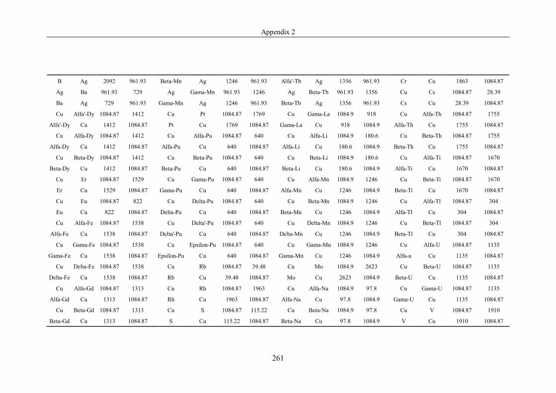
Appendix 2
261
B Ag 2092 961.93 Beta-Mn Ag 1246 961.93 Alfa'-Tb Ag 1356 961.93 Cr Cu 1863 1084.87
Ag Ba 961.93 729 Ag Gama-Mn 961.93 1246 Ag Beta-Tb 961.93 1356 Cu Cs 1084.87 28.39
Ba Ag 729 961.93 Gama-Mn Ag 1246 961.93 Beta-Tb Ag 1356 961.93 Cs Cu 28.39 1084.87
Cu Alfa'-Dy 1084.87 1412 Cu Pt 1084.87 1769 Cu Gama-La 1084.9 918 Cu Alfa-Th 1084.87 1755
Alfa'-Dy Cu 1412 1084.87 Pt Cu 1769 1084.87 Gama-La Cu 918 1084.9 Alfa-Th Cu 1755 1084.87
Cu Alfa-Dy 1084.87 1412 Cu Alfa-Pu 1084.87 640 Cu Alfa-Li 1084.9 180.6 Cu Beta-Th 1084.87 1755
Alfa-Dy Cu 1412 1084.87 Alfa-Pu Cu 640 1084.87 Alfa-Li Cu 180.6 1084.9 Beta-Th Cu 1755 1084.87
Cu Beta-Dy 1084.87 1412 Cu Beta-Pu 1084.87 640 Cu Beta-Li 1084.9 180.6 Cu Alfa-Ti 1084.87 1670
Beta-Dy Cu 1412 1084.87 Beta-Pu Cu 640 1084.87 Beta-Li Cu 180.6 1084.9 Alfa-Ti Cu 1670 1084.87
Cu Er 1084.87 1529 Cu Gama-Pu 1084.87 640 Cu Alfa-Mn 1084.9 1246 Cu Beta-Ti 1084.87 1670
Er Cu 1529 1084.87 Gama-Pu Cu 640 1084.87 Alfa-Mn Cu 1246 1084.9 Beta-Ti Cu 1670 1084.87
Cu Eu 1084.87 822 Cu Delta-Pu 1084.87 640 Cu Beta-Mn 1084.9 1246 Cu Alfa-Tl 1084.87 304
Eu Cu 822 1084.87 Delta-Pu Cu 640 1084.87 Beta-Mn Cu 1246 1084.9 Alfa-Tl Cu 304 1084.87
Cu Alfa-Fe 1084.87 1538 Cu Delta'-Pu 1084.87 640 Cu Delta-Mn 1084.9 1246 Cu Beta-Tl 1084.87 304
Alfa-Fe Cu 1538 1084.87 Delta'-Pu Cu 640 1084.87 Delta-Mn Cu 1246 1084.9 Beta-Tl Cu 304 1084.87
Cu Gama-Fe 1084.87 1538 Cu Epsilon-Pu 1084.87 640 Cu Gama-Mn 1084.9 1246 Cu Alfa-U 1084.87 1135
Gama-Fe Cu 1538 1084.87 Epsilon-Pu Cu 640 1084.87 Gama-Mn Cu 1246 1084.9 Alfa-u Cu 1135 1084.87
Cu Delta-Fe 1084.87 1538 Cu Rb 1084.87 39.48 Cu Mo 1084.9 2623 Cu Beta-U 1084.87 1135
Delta-Fe Cu 1538 1084.87 Rb Cu 39.48 1084.87 Mo Cu 2623 1084.9 Beta-U Cu 1135 1084.87
Cu Alfa-Gd 1084.87 1313 Cu Rh 1084.87 1963 Cu Alfa-Na 1084.9 97.8 Cu Gama-U 1084.87 1135
Alfa-Gd Cu 1313 1084.87 Rh Cu 1963 1084.87 Alfa-Na Cu 97.8 1084.9 Gama-U Cu 1135 1084.87
Cu Beta-Gd 1084.87 1313 Cu S 1084.87 115.22 Cu Beta-Na 1084.9 97.8 Cu V 1084.87 1910
Beta-Gd Cu 1313 1084.87 S Cu 115.22 1084.87 Beta-Na Cu 97.8 1084.9 V Cu 1910 1084.87
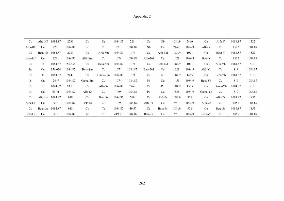
Appendix 2
262
Cu Alfa-Hf 1084.87 2231 Cu Se 1084.87 221 Cu Nb 1084.9 2469 Cu Alfa-Y 1084.87 1522
Alfa-Hf Cu 2231 1084.87 Se Cu 221 1084.87 Nb Cu 2469 1084.9 Alfa-Y Cu 1522 1084.87
Cu Beta-Hf 1084.87 2231 Cu Alfa-Sm 1084.87 1074 Cu Alfa-Nd 1084.9 1021 Cu Beta-Y 1084.87 1522
Beta-Hf Cu 2231 1084.87 Alfa-Sm Cu 1074 1084.87 Alfa-Nd Cu 1021 1084.9 Beta-Y Cu 1522 1084.87
Cu In 1084.87 156.634 Cu Beta-Sm 1084.87 1074 Cu Beta-Nd 1084.9 1021 Cu Alfa-Yb 1084.87 819
In Cu 156.634 1084.87 Beta-Sm Cu 1074 1084.87 Beta-Nd Cu 1021 1084.9 Alfa-Yb Cu 819 1084.87
Cu Ir 1084.87 2447 Cu Gama-Sm 1084.87 1074 Cu Ni 1084.9 1455 Cu Beta-Yb 1084.87 819
Ir Cu 2447 1084.87 Gama-Sm Cu 1074 1084.87 Ni Cu 1455 1084.9 Beta-Yb Cu 819 1084.87
Cu K 1084.87 63.71 Cu Alfa-Sr 1084.87 7769 Cu Pd 1084.9 1555 Cu Gama-Yb 1084.87 819
K Cu 63.71 1084.87 Alfa-Sr Cu 769 1084.87 Pd Cu 1555 1084.9 Gama-Yb Cu 819 1084.87
Cu Alfa-La 1084.87 918 Cu Beta-Sr 1084.87 769 Cu Alfa-Pr 1084.9 931 Cu Alfa-Zr 1084.87 1855
Alfa-La Cu 918 1084.87 Beta-Sr Cu 769 1084.87 Alfa-Pr Cu 931 1084.9 Alfa-Zr Cu 1855 1084.87
Cu Beta-La 1084.87 918 Cu Te 1084.87 449.57 Cu Beta-Pr 1084.9 931 Cu Beta-Zr 1084.87 1855
Beta-La Cu 918 1084.87 Te Cu 449.57 1084.87 Beta-Pr Cu 931 1084.9 Beta-Zr Cu 1855 1084.87
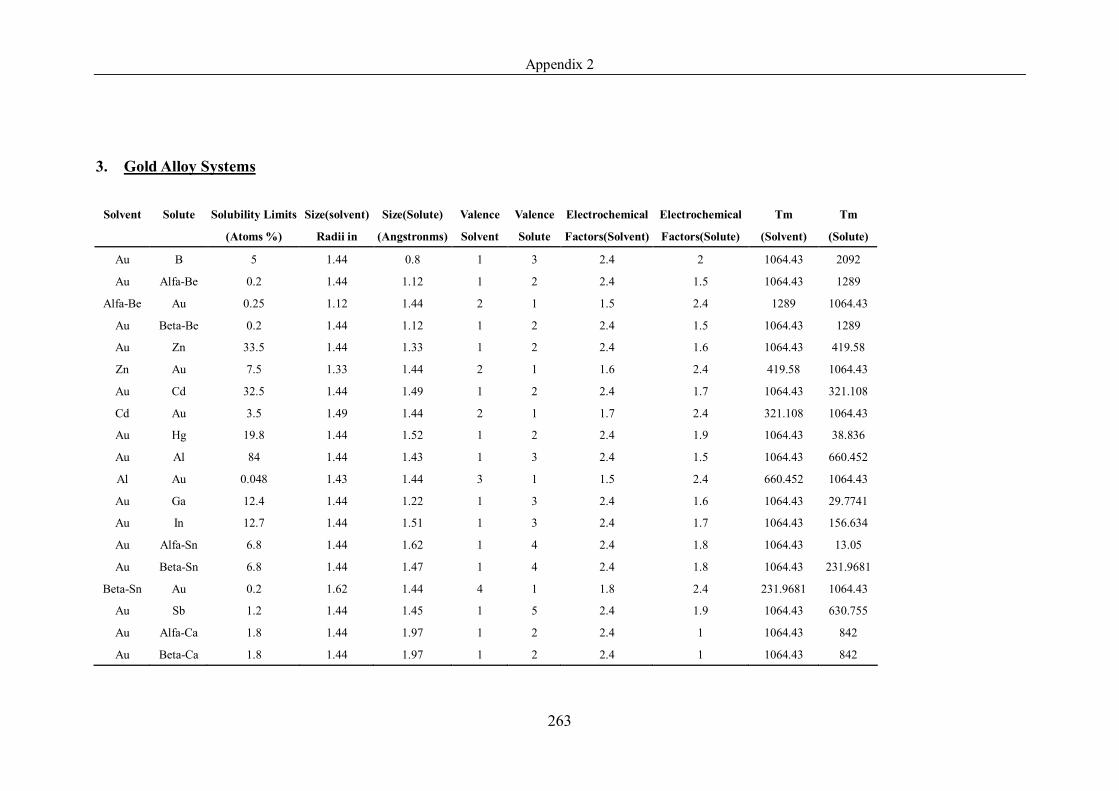
Appendix 2
263
3. Gold Alloy Systems
Solvent Solute Solubility Limits Size(solvent) Size(Solute) Valence Valence Electrochemical Electrochemical Tm Tm
(Atoms %) Radii in (Angstronms) Solvent Solute Factors(Solvent) Factors(Solute) (Solvent) (Solute)
Au B 5 1.44 0.8 1 3 2.4 2 1064.43 2092
Au Alfa-Be 0.2 1.44 1.12 1 2 2.4 1.5 1064.43 1289
Alfa-Be Au 0.25 1.12 1.44 2 1 1.5 2.4 1289 1064.43
Au Beta-Be 0.2 1.44 1.12 1 2 2.4 1.5 1064.43 1289
Au Zn 33.5 1.44 1.33 1 2 2.4 1.6 1064.43 419.58
Zn Au 7.5 1.33 1.44 2 1 1.6 2.4 419.58 1064.43
Au Cd 32.5 1.44 1.49 1 2 2.4 1.7 1064.43 321.108
Cd Au 3.5 1.49 1.44 2 1 1.7 2.4 321.108 1064.43
Au Hg 19.8 1.44 1.52 1 2 2.4 1.9 1064.43 38.836
Au Al 84 1.44 1.43 1 3 2.4 1.5 1064.43 660.452
Al Au 0.048 1.43 1.44 3 1 1.5 2.4 660.452 1064.43
Au Ga 12.4 1.44 1.22 1 3 2.4 1.6 1064.43 29.7741
Au In 12.7 1.44 1.51 1 3 2.4 1.7 1064.43 156.634
Au Alfa-Sn 6.8 1.44 1.62 1 4 2.4 1.8 1064.43 13.05
Au Beta-Sn 6.8 1.44 1.47 1 4 2.4 1.8 1064.43 231.9681
Beta-Sn Au 0.2 1.62 1.44 4 1 1.8 2.4 231.9681 1064.43
Au Sb 1.2 1.44 1.45 1 5 2.4 1.9 1064.43 630.755
Au Alfa-Ca 1.8 1.44 1.97 1 2 2.4 1 1064.43 842
Au Beta-Ca 1.8 1.44 1.97 1 2 2.4 1 1064.43 842
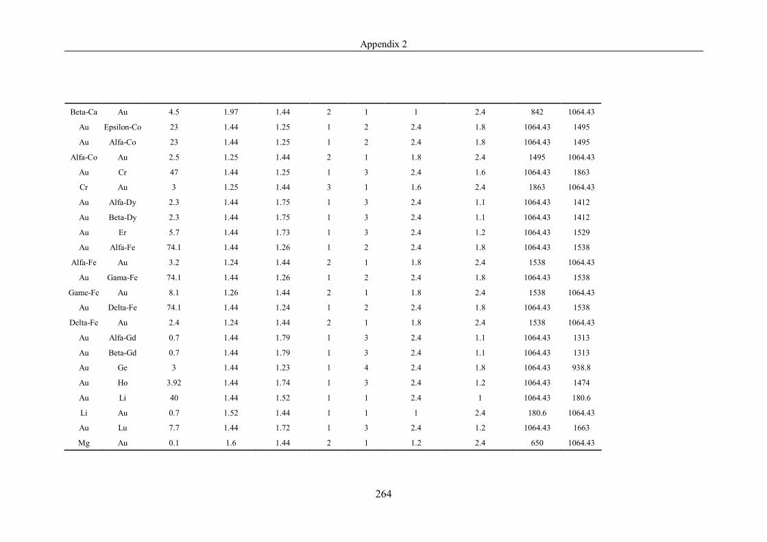
Appendix 2
264
Beta-Ca Au 4.5 1.97 1.44 2 1 1 2.4 842 1064.43
Au Epsilon-Co 23 1.44 1.25 1 2 2.4 1.8 1064.43 1495
Au Alfa-Co 23 1.44 1.25 1 2 2.4 1.8 1064.43 1495
Alfa-Co Au 2.5 1.25 1.44 2 1 1.8 2.4 1495 1064.43
Au Cr 47 1.44 1.25 1 3 2.4 1.6 1064.43 1863
Cr Au 3 1.25 1.44 3 1 1.6 2.4 1863 1064.43
Au Alfa-Dy 2.3 1.44 1.75 1 3 2.4 1.1 1064.43 1412
Au Beta-Dy 2.3 1.44 1.75 1 3 2.4 1.1 1064.43 1412
Au Er 5.7 1.44 1.73 1 3 2.4 1.2 1064.43 1529
Au Alfa-Fe 74.1 1.44 1.26 1 2 2.4 1.8 1064.43 1538
Alfa-Fe Au 3.2 1.24 1.44 2 1 1.8 2.4 1538 1064.43
Au Gama-Fe 74.1 1.44 1.26 1 2 2.4 1.8 1064.43 1538
Game-Fe Au 8.1 1.26 1.44 2 1 1.8 2.4 1538 1064.43
Au Delta-Fe 74.1 1.44 1.24 1 2 2.4 1.8 1064.43 1538
Delta-Fe Au 2.4 1.24 1.44 2 1 1.8 2.4 1538 1064.43
Au Alfa-Gd 0.7 1.44 1.79 1 3 2.4 1.1 1064.43 1313
Au Beta-Gd 0.7 1.44 1.79 1 3 2.4 1.1 1064.43 1313
Au Ge 3 1.44 1.23 1 4 2.4 1.8 1064.43 938.8
Au Ho 3.92 1.44 1.74 1 3 2.4 1.2 1064.43 1474
Au Li 40 1.44 1.52 1 1 2.4 1 1064.43 180.6
Li Au 0.7 1.52 1.44 1 1 1 2.4 180.6 1064.43
Au Lu 7.7 1.44 1.72 1 3 2.4 1.2 1064.43 1663
Mg Au 0.1 1.6 1.44 2 1 1.2 2.4 650 1064.43
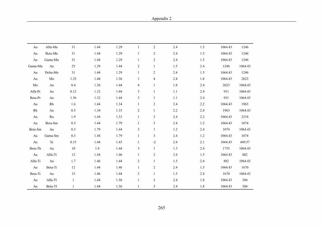
Appendix 2
265
Au Alfa-Mn 31 1.44 1.29 1 2 2.4 1.5 1064.43 1246
Au Beta-Mn 31 1.44 1.29 1 2 2.4 1.5 1064.43 1246
Au Gama-Mn 31 1.44 1.29 1 2 2.4 1.5 1064.43 1246
Gama-Mn Au 25 1.29 1.44 2 1 1.5 2.4 1246 1064.43
Au Delta-Mn 31 1.44 1.29 1 2 2.4 1.5 1064.43 1246
Au Mo 1.25 1.44 1.36 1 4 2.4 1.8 1064.43 2623
Mo Au 0.4 1.36 1.44 4 1 1.8 2.4 2623 1064.43
Alfa-Pr Au 0.12 1.32 1.44 3 1 1.1 2.4 931 1064.43
Beta-Pr Au 1.56 1.32 1.44 3 1 1.1 2.4 931 1064.43
Au Rh 1.6 1.44 1.34 1 2 2.4 2.2 1064.43 1963
Rh Au 0.5 1.34 1.33 2 1 2.2 2.4 1963 1064.43
Au Ru 1.9 1.44 1.33 1 3 2.4 2.2 1064.43 2334
Au Beta-Sm 0.3 1.44 1.79 1 3 2.4 1.2 1064.43 1074
Beta-Sm Au 0.3 1.79 1.44 3 1 1.2 2.4 1074 1064.43
Au Gama-Sm 0.3 1.44 1.79 1 3 2.4 1.2 1064.43 1074
Au Te 0.15 1.44 1.43 1 -2 2.4 2.1 1064.43 449.57
Beta-Th Au 10 1.8 1.44 3 1 1.3 2.4 1755 1064.43
Au Alfa-Ti 12 1.44 1.46 1 2 2.4 1.5 1064.43 882
Alfa-Ti Au 1.7 1.46 1.44 2 1 1.5 2.4 882 1064.43
Au Beta-Ti 12 1.44 1.46 1 2 2.4 1.5 1064.43 1670
Beta-Ti Au 15 1.46 1.44 2 1 1.5 2.4 1670 1064.43
Au Alfa-Tl 1 1.44 1.56 1 3 2.4 1.8 1064.43 304
Au Beta-Tl 1 1.44 1.56 1 3 2.4 1.8 1064.43 304
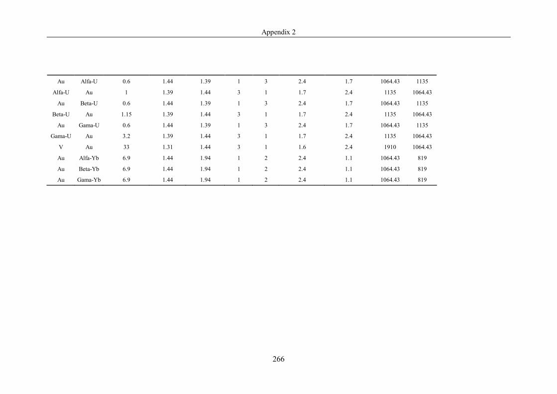
Appendix 2
266
Au Alfa-U 0.6 1.44 1.39 1 3 2.4 1.7 1064.43 1135
Alfa-U Au 1 1.39 1.44 3 1 1.7 2.4 1135 1064.43
Au Beta-U 0.6 1.44 1.39 1 3 2.4 1.7 1064.43 1135
Beta-U Au 1.15 1.39 1.44 3 1 1.7 2.4 1135 1064.43
Au Gama-U 0.6 1.44 1.39 1 3 2.4 1.7 1064.43 1135
Gama-U Au 3.2 1.39 1.44 3 1 1.7 2.4 1135 1064.43
V Au 33 1.31 1.44 3 1 1.6 2.4 1910 1064.43
Au Alfa-Yb 6.9 1.44 1.94 1 2 2.4 1.1 1064.43 819
Au Beta-Yb 6.9 1.44 1.94 1 2 2.4 1.1 1064.43 819
Au Gama-Yb 6.9 1.44 1.94 1 2 2.4 1.1 1064.43 819
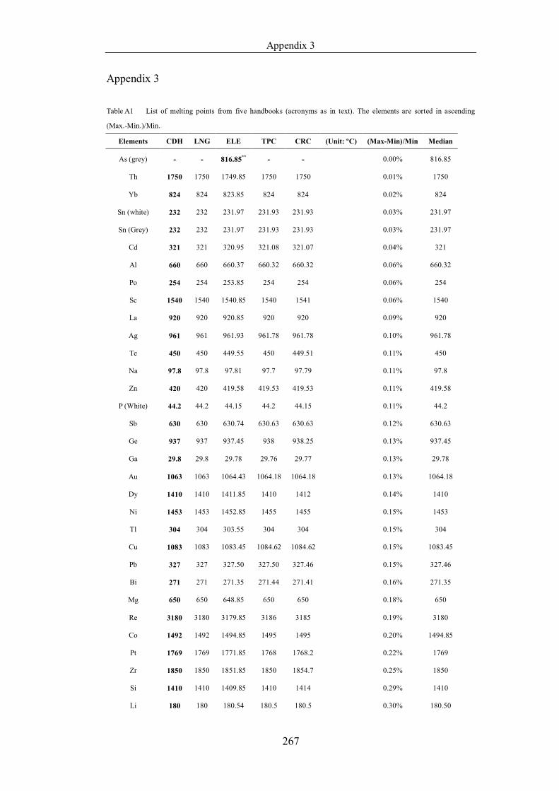
Appendix 3
267
Appendix 3 Table A1 List of melting points from five handbooks (acronyms as in text). The elements are sorted in ascending
(Max.-Min.)/Min.
Elements CDH LNG ELE TPC CRC (Unit: ºC) (Max-Min)/Min Median
As (grey) - - 816.85** - - 0.00% 816.85
Th 1750 1750 1749.85 1750 1750 0.01% 1750
Yb 824 824 823.85 824 824 0.02% 824
Sn (white) 232 232 231.97 231.93 231.93 0.03% 231.97
Sn (Grey) 232 232 231.97 231.93 231.93 0.03% 231.97
Cd 321 321 320.95 321.08 321.07 0.04% 321
Al 660 660 660.37 660.32 660.32 0.06% 660.32
Po 254 254 253.85 254 254 0.06% 254
Sc 1540 1540 1540.85 1540 1541 0.06% 1540
La 920 920 920.85 920 920 0.09% 920
Ag 961 961 961.93 961.78 961.78 0.10% 961.78
Te 450 450 449.55 450 449.51 0.11% 450
Na 97.8 97.8 97.81 97.7 97.79 0.11% 97.8
Zn 420 420 419.58 419.53 419.53 0.11% 419.58
P (White) 44.2 44.2 44.15 44.2 44.15 0.11% 44.2
Sb 630 630 630.74 630.63 630.63 0.12% 630.63
Ge 937 937 937.45 938 938.25 0.13% 937.45
Ga 29.8 29.8 29.78 29.76 29.77 0.13% 29.78
Au 1063 1063 1064.43 1064.18 1064.18 0.13% 1064.18
Dy 1410 1410 1411.85 1410 1412 0.14% 1410
Ni 1453 1453 1452.85 1455 1455 0.15% 1453
Tl 304 304 303.55 304 304 0.15% 304
Cu 1083 1083 1083.45 1084.62 1084.62 0.15% 1083.45
Pb 327 327 327.50 327.50 327.46 0.15% 327.46
Bi 271 271 271.35 271.44 271.41 0.16% 271.35
Mg 650 650 648.85 650 650 0.18% 650
Re 3180 3180 3179.85 3186 3185 0.19% 3180
Co 1492 1492 1494.85 1495 1495 0.20% 1494.85
Pt 1769 1769 1771.85 1768 1768.2 0.22% 1769
Zr 1850 1850 1851.85 1850 1854.7 0.25% 1850
Si 1410 1410 1409.85 1410 1414 0.29% 1410
Li 180 180 180.54 180.5 180.5 0.30% 180.50
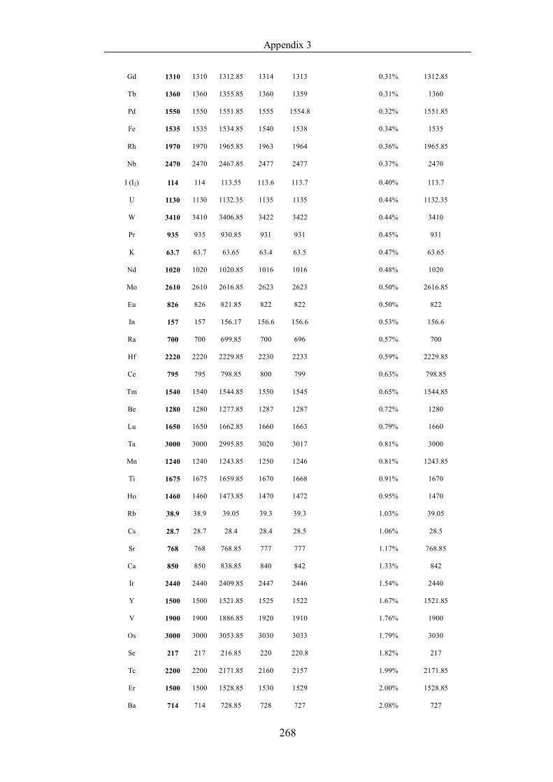
Appendix 3
268
Gd 1310 1310 1312.85 1314 1313 0.31% 1312.85
Tb 1360 1360 1355.85 1360 1359 0.31% 1360
Pd 1550 1550 1551.85 1555 1554.8 0.32% 1551.85
Fe 1535 1535 1534.85 1540 1538 0.34% 1535
Rh 1970 1970 1965.85 1963 1964 0.36% 1965.85
Nb 2470 2470 2467.85 2477 2477 0.37% 2470
I (I2) 114 114 113.55 113.6 113.7 0.40% 113.7
U 1130 1130 1132.35 1135 1135 0.44% 1132.35
W 3410 3410 3406.85 3422 3422 0.44% 3410
Pr 935 935 930.85 931 931 0.45% 931
K 63.7 63.7 63.65 63.4 63.5 0.47% 63.65
Nd 1020 1020 1020.85 1016 1016 0.48% 1020
Mo 2610 2610 2616.85 2623 2623 0.50% 2616.85
Eu 826 826 821.85 822 822 0.50% 822
In 157 157 156.17 156.6 156.6 0.53% 156.6
Ra 700 700 699.85 700 696 0.57% 700
Hf 2220 2220 2229.85 2230 2233 0.59% 2229.85
Ce 795 795 798.85 800 799 0.63% 798.85
Tm 1540 1540 1544.85 1550 1545 0.65% 1544.85
Be 1280 1280 1277.85 1287 1287 0.72% 1280
Lu 1650 1650 1662.85 1660 1663 0.79% 1660
Ta 3000 3000 2995.85 3020 3017 0.81% 3000
Mn 1240 1240 1243.85 1250 1246 0.81% 1243.85
Ti 1675 1675 1659.85 1670 1668 0.91% 1670
Ho 1460 1460 1473.85 1470 1472 0.95% 1470
Rb 38.9 38.9 39.05 39.3 39.3 1.03% 39.05
Cs 28.7 28.7 28.4 28.4 28.5 1.06% 28.5
Sr 768 768 768.85 777 777 1.17% 768.85
Ca 850 850 838.85 840 842 1.33% 842
Ir 2440 2440 2409.85 2447 2446 1.54% 2440
Y 1500 1500 1521.85 1525 1522 1.67% 1521.85
V 1900 1900 1886.85 1920 1910 1.76% 1900
Os 3000 3000 3053.85 3030 3033 1.79% 3030
Se 217 217 216.85 220 220.8 1.82% 217
Tc 2200 2200 2171.85 2160 2157 1.99% 2171.85
Er 1500 1500 1528.85 1530 1529 2.00% 1528.85
Ba 714 714 728.85 728 727 2.08% 727
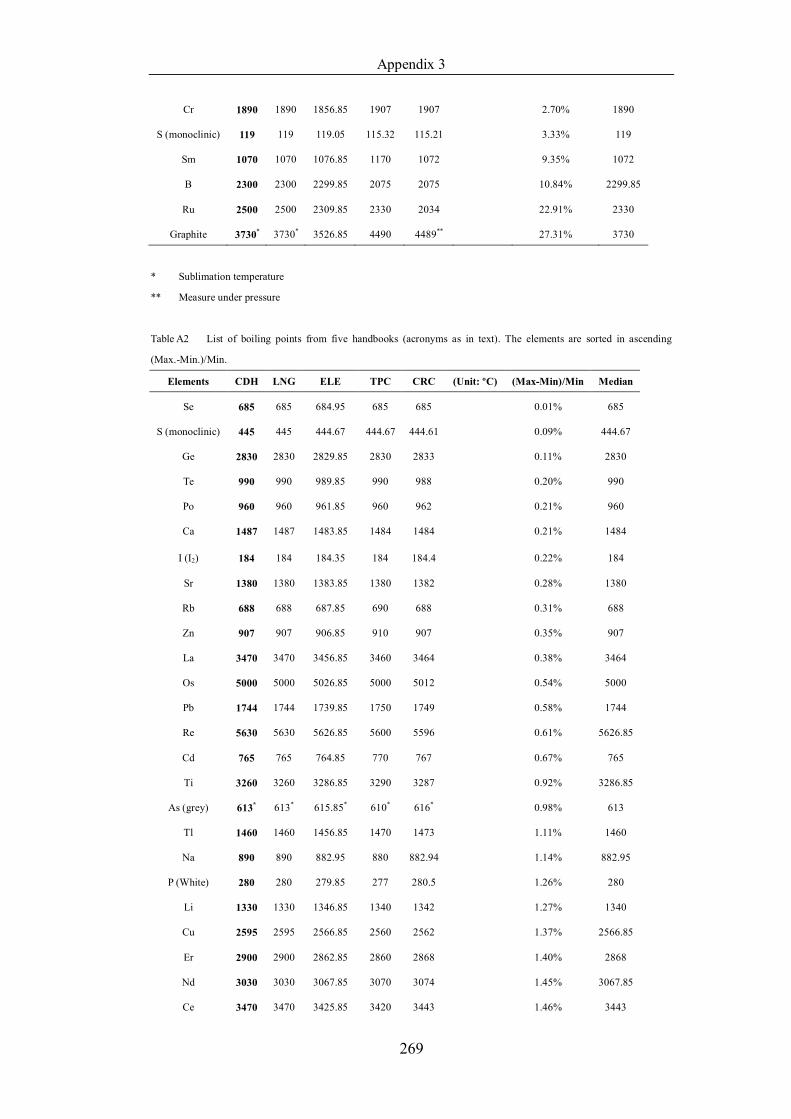
Appendix 3
269
Cr 1890 1890 1856.85 1907 1907 2.70% 1890
S (monoclinic) 119 119 119.05 115.32 115.21 3.33% 119
Sm 1070 1070 1076.85 1170 1072 9.35% 1072
B 2300 2300 2299.85 2075 2075 10.84% 2299.85
Ru 2500 2500 2309.85 2330 2034 22.91% 2330
Graphite 3730* 3730* 3526.85 4490 4489** 27.31% 3730
* Sublimation temperature
** Measure under pressure
Table A2 List of boiling points from five handbooks (acronyms as in text). The elements are sorted in ascending
(Max.-Min.)/Min.
Elements CDH LNG ELE TPC CRC (Unit: ºC) (Max-Min)/Min Median
Se 685 685 684.95 685 685 0.01% 685
S (monoclinic) 445 445 444.67 444.67 444.61 0.09% 444.67
Ge 2830 2830 2829.85 2830 2833 0.11% 2830
Te 990 990 989.85 990 988 0.20% 990
Po 960 960 961.85 960 962 0.21% 960
Ca 1487 1487 1483.85 1484 1484 0.21% 1484
I (I2) 184 184 184.35 184 184.4 0.22% 184
Sr 1380 1380 1383.85 1380 1382 0.28% 1380
Rb 688 688 687.85 690 688 0.31% 688
Zn 907 907 906.85 910 907 0.35% 907
La 3470 3470 3456.85 3460 3464 0.38% 3464
Os 5000 5000 5026.85 5000 5012 0.54% 5000
Pb 1744 1744 1739.85 1750 1749 0.58% 1744
Re 5630 5630 5626.85 5600 5596 0.61% 5626.85
Cd 765 765 764.85 770 767 0.67% 765
Ti 3260 3260 3286.85 3290 3287 0.92% 3286.85
As (grey) 613* 613* 615.85* 610* 616* 0.98% 613
Tl 1460 1460 1456.85 1470 1473 1.11% 1460
Na 890 890 882.95 880 882.94 1.14% 882.95
P (White) 280 280 279.85 277 280.5 1.26% 280
Li 1330 1330 1346.85 1340 1342 1.27% 1340
Cu 2595 2595 2566.85 2560 2562 1.37% 2566.85
Er 2900 2900 2862.85 2860 2868 1.40% 2868
Nd 3030 3030 3067.85 3070 3074 1.45% 3067.85
Ce 3470 3470 3425.85 3420 3443 1.46% 3443
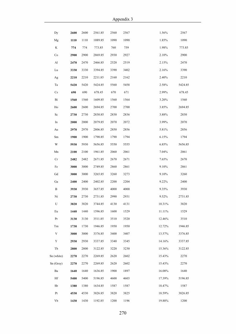
Appendix 3
270
Dy 2600 2600 2561.85 2560 2567 1.56% 2567
Mg 1110 1110 1089.85 1090 1090 1.85% 1090
K 774 774 773.85 760 759 1.98% 773.85
Co 2900 2900 2869.85 2930 2927 2.10% 2900
Al 2470 2470 2466.85 2520 2519 2.15% 2470
Lu 3330 3330 3394.85 3390 3402 2.16% 3390
Ag 2210 2210 2211.85 2160 2162 2.40% 2210
Ta 5420 5420 5424.85 5560 5458 2.58% 5424.85
Cs 690 690 678.45 670 671 2.99% 678.45
Bi 1560 1560 1609.85 1560 1564 3.20% 1560
Ho 2600 2600 2694.85 2700 2700 3.85% 2694.85
Sc 2730 2730 2830.85 2830 2836 3.88% 2830
In 2000 2000 2079.85 2070 2072 3.99% 2070
Au 2970 2970 2806.85 2850 2856 5.81% 2856
Sm 1900 1900 1790.85 1790 1794 6.15% 1794
W 5930 5930 5656.85 5550 5555 6.85% 5656.85
Mn 2100 2100 1961.85 2060 2061 7.04% 2061
Cr 2482 2482 2671.85 2670 2671 7.65% 2670
Fe 3000 3000 2749.85 2860 2861 9.10% 2861
Gd 3000 3000 3265.85 3260 3273 9.10% 3260
Ga 2400 2400 2402.85 2200 2204 9.22% 2400
B 3930 3930 3657.85 4000 4000 9.35% 3930
Ni 2730 2730 2731.85 2990 2931 9.52% 2731.85
U 3820 3820 3744.85 4130 4131 10.31% 3820
Eu 1440 1440 1596.85 1600 1529 11.11% 1529
Pr 3130 3130 3511.85 3510 3520 12.46% 3510
Tm 1730 1730 1946.85 1950 1950 12.72% 1946.85
V 3000 3000 3376.85 3400 3407 13.57% 3376.85
Y 2930 2930 3337.85 3340 3345 14.16% 3337.85
Tb 2800 2800 3122.85 3220 3230 15.36% 3122.85
Sn (white) 2270 2270 2269.85 2620 2602 15.43% 2270
Sn (Grey) 2270 2270 2269.85 2620 2602 15.43% 2270
Ba 1640 1640 1636.85 1900 1897 16.08% 1640
Hf 5400 5400 5196.85 4600 4603 17.39% 5196.85
Sb 1380 1380 1634.85 1587 1587 18.47% 1587
Pt 4530 4530 3826.85 3820 3825 18.59% 3826.85
Yb 1430 1430 1192.85 1200 1196 19.88% 1200
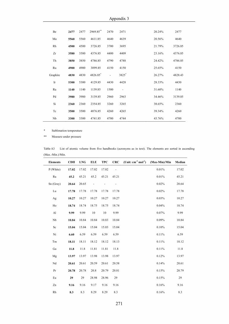
Appendix 3
271
Be 2477 2477 2969.85** 2470 2471 20.24% 2477
Mo 5560 5560 4611.85 4640 4639 20.56% 4640
Rh 4500 4500 3726.85 3700 3695 21.79% 3726.85
Zr 3580 3580 4376.85 4400 4409 23.16% 4376.85
Th 3850 3850 4786.85 4790 4788 24.42% 4786.85
Ru 4900 4900 3899.85 4150 4150 25.65% 4150
Graphite 4830 4830 4826.85* - 3825* 26.27% 4828.43
Ir 5300 5300 4129.85 4430 4428 28.33% 4430
Ra 1140 1140 1139.85 1500 - 31.60% 1140
Pd 3980 3980 3139.85 2960 2963 34.46% 3139.85
Si 2360 2360 2354.85 3260 3265 38.65% 2360
Tc 3500 3500 4876.85 4260 4265 39.34% 4260
Nb 3300 3300 4741.85 4700 4744 43.76% 4700
* Sublimation temperature
** Measure under pressure
Table A3 List of atomic volume from five handbooks (acronyms as in text). The elements are sorted in ascending
(Max.-Min.)/Min.
Elements CDH LNG ELE TPC CRC (Unit: cm-3 mol-1) (Max-Min)/Min Median
P (White) 17.02 17.02 17.02 17.02 - 0.01% 17.02
Ra 45.2 45.21 45.2 45.21 45.21 0.01% 45.21
Sn (Grey) 20.64 20.65 - - - 0.02% 20.64
Lu 17.78 17.78 17.78 17.78 17.78 0.02% 17.78
Ag 10.27 10.27 10.27 10.27 10.27 0.03% 10.27
Ho 18.74 18.74 18.75 18.75 18.74 0.04% 18.74
Al 9.99 9.99 10 10 9.99 0.07% 9.99
Nb 10.84 10.84 10.84 10.83 10.84 0.09% 10.84
Sc 15.04 15.04 15.04 15.03 15.04 0.10% 15.04
Ni 6.60 6.59 6.59 6.59 6.59 0.11% 6.59
Tm 18.11 18.11 18.12 18.12 18.13 0.11% 18.12
Ga 11.8 11.8 11.81 11.81 11.8 0.11% 11.8
Mg 13.97 13.97 13.98 13.98 13.97 0.12% 13.97
Nd 20.61 20.61 20.59 20.61 20.58 0.14% 20.61
Pr 20.78 20.78 20.8 20.79 20.81 0.15% 20.79
Eu 29 29 28.98 28.96 29 0.15% 29
Zn 9.16 9.16 9.17 9.16 9.16 0.16% 9.16
Rh 8.3 8.3 8.29 8.29 8.3 0.16% 8.3

Appendix 3
272
Rb 55.86 55.86 55.79 55.75 55.86 0.20% 55.86
Th 19.83 19.83 19.8 19.79 19.83 0.21% 19.83
Fe 7.11 7.11 7.09 7.09 7.1 0.21% 7.1
Be 4.87 4.87 4.88 4.88 4.87 0.22% 4.87
Mo 9.41 9.41 9.39 9.39 9.41 0.24% 9.41
Pd 8.87 8.87 8.85 8.87 8.87 0.25% 8.87
Au 10.21 10.21 10.19 10.22 10.21 0.25% 10.21
Hf 13.42 13.42 13.41 13.44 13.42 0.26% 13.42
In 15.73 15.73 15.71 15.75 15.71 0.27% 15.73
Sm 19.95 19.94 20 19.95 19.99 0.29% 19.95
Dy 18.98 18.98 19 19.05 19.01 0.34% 19
Os 8.45 8.45 8.43 8.42 8.42 0.38% 8.43
Pb 18.34 18.34 18.26 18.27 18.34 0.42% 18.34
Zr 14.06 14.06 14.02 14.02 13.99 0.46% 14.02
I (I2) 25.74 25.74 25.74 25.62 - 0.47% 25.74
Pt 9.12 9.12 9.10 9.09 9.07 0.47% 9.10
Cu 7.12 7.12 7.09 7.11 7.09 0.48% 7.11
Tb 19.22 19.22 19.31 19.22 19.31 0.49% 19.22
Na 23.7 23.7 23.68 23.8 23.7 0.50% 23.7
Ir 8.54 8.54 8.57 8.52 8.54 0.54% 8.54
Bi 21.32 21.32 21.44 21.32 21.35 0.57% 21.32
Cd 13.01 13.01 13 13 12.94 0.58% 13
Tl 17.32 17.32 17.24 17.22 17.32 0.60% 17.32
Cr 7.23 7.23 7.23 7.23 7.27 0.62% 7.23
Sn (white) 16.30 16.31 16.24 16.3 16.35 0.68% 16.3
Ti 10.55 10.55 10.55 10.62 10.61 0.71% 10.55
Graphite 5.34 5.34 - 5.3 - 0.71% 5.34
La 22.44 22.44 22.6 22.5 22.59 0.71% 22.5
W 9.48 9.48 9.53 9.55 9.53 0.75% 9.53
Li 13.1 13.1 13 13.02 13 0.75% 13.02
U 12.46 12.46 12.56 12.49 12.46 0.78% 12.46
Gd 19.78 19.78 19.9 19.98 19.91 1.02% 19.9
Sb 18.39 18.39 18.20 18.19 18.23 1.08% 18.23
Co 6.62 6.62 6.62 6.7 6.65 1.16% 6.62
Yb 24.79 24.79 24.84 24.84 25.08 1.17% 24.84
Er 18.26 18.26 18.44 18.49 18.44 1.28% 18.44
Ca 26.03 26.03 25.86 26.19 26.02 1.29% 26.03
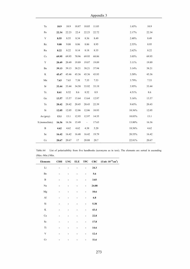
Appendix 3
273
Ta 10.9 10.9 10.87 10.85 11.03 1.65% 10.9
Po 22.34 22.23 22.4 22.23 22.72 2.17% 22.34
V 8.55 8.55 8.34 8.36 8.49 2.48% 8.49
Re 9.08 9.08 8.86 8.86 8.95 2.55% 8.95
Ru 8.22 8.22 8.14 8.18 8.35 2.62% 8.22
Cs 69.95 69.95 70.96 69.95 68.86 3.05% 69.95
Y 20.49 20.49 19.89 19.87 19.89 3.11% 19.89
Ba 39.13 39.13 38.21 38.21 37.94 3.14% 38.21
K 45.47 45.46 45.36 45.36 43.93 3.50% 45.36
Mn 7.63 7.63 7.38 7.35 7.53 3.79% 7.53
Sr 33.44 33.44 34.50 33.92 33.19 3.95% 33.44
Tc 8.61 8.52 8.6 8.52 8.9 4.51% 8.6
Ge 13.57 13.57 13.64 13.64 12.97 5.16% 13.57
Te 20.42 20.42 20.45 20.43 22.39 9.65% 20.43
Si 12.05 12.05 12.06 12.06 10.93 10.36% 12.05
As (grey) 13.1 13.1 12.95 12.97 14.35 10.83% 13.1
S (monoclinic) 16.36 16.36 15.49 - 17.63 13.80% 16.36
B 4.62 4.62 4.62 4.38 5.20 18.56% 4.62
Se 16.42 16.42 16.48 16.42 19.79 20.55% 16.42
Ce 20.67 20.67 17 20.88 20.7 22.81% 20.67
Table A4 List of polarizability from five handbooks (acronyms as in text). The elements are sorted in ascending
(Max.-Min.)/Min.
Elements CDH LNG ELE TPC CRC (Unit: 10-24cm3)
Li - - - - 24.3
Be - - - - 5.6
B - - - - 3.03
Na - - - - 24.08
Mg - - - - 10.6
Al - - - - 6.8
Si - - - - 5.38
K - - - - 43.4
Ca - - - - 22.8
Sc - - - - 17.8
Ti - - - - 14.6
V - - - - 12.4
Cr - - - - 11.6
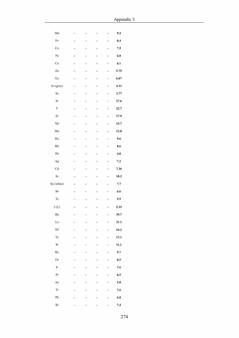
Appendix 3
274
Mn - - - - 9.4
Fe - - - - 8.4
Co - - - - 7.5
Ni - - - - 6.8
Cu - - - - 6.1
Zn - - - - 5.75
Ge - - - - 6.07
As (grey) - - - - 4.31
Se - - - - 3.77
Sr - - - - 27.6
Y - - - - 22.7
Zr - - - - 17.9
Nb - - - - 15.7
Mo - - - - 12.8
Ru - - - - 9.6
Rh - - - - 8.6
Pd - - - - 4.8
Ag - - - - 7.2
Cd - - - - 7.36
In - - - - 10.2
Sn (white) - - - - 7.7
Sb - - - - 6.6
Te - - - - 5.5
I (I2) - - - - 5.35
Ba - - - - 39.7
La - - - - 31.1
Hf - - - - 16.2
Ta - - - - 13.1
W - - - - 11.1
Re - - - - 9.7
Os - - - - 8.5
Ir - - - - 7.6
Pt - - - - 6.5
Au - - - - 5.8
Tl - - - - 7.6
Pb - - - - 6.8
Bi - - - - 7.4
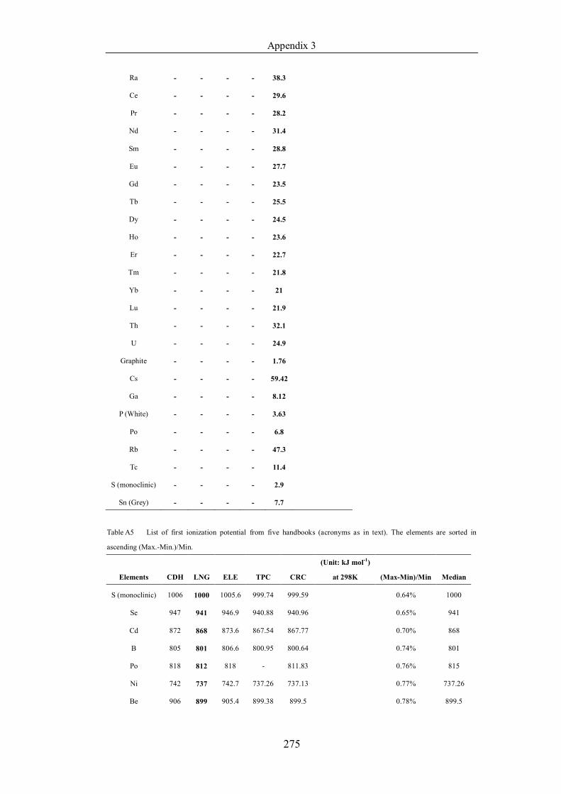
Appendix 3
275
Ra - - - - 38.3
Ce - - - - 29.6
Pr - - - - 28.2
Nd - - - - 31.4
Sm - - - - 28.8
Eu - - - - 27.7
Gd - - - - 23.5
Tb - - - - 25.5
Dy - - - - 24.5
Ho - - - - 23.6
Er - - - - 22.7
Tm - - - - 21.8
Yb - - - - 21
Lu - - - - 21.9
Th - - - - 32.1
U - - - - 24.9
Graphite - - - - 1.76
Cs - - - - 59.42
Ga - - - - 8.12
P (White) - - - - 3.63
Po - - - - 6.8
Rb - - - - 47.3
Tc - - - - 11.4
S (monoclinic) - - - - 2.9
Sn (Grey) - - - - 7.7
Table A5 List of first ionization potential from five handbooks (acronyms as in text). The elements are sorted in
ascending (Max.-Min.)/Min.
Elements CDH LNG ELE TPC CRC
(Unit: kJ mol-1)
at 298K (Max-Min)/Min Median
S (monoclinic) 1006 1000 1005.6 999.74 999.59 0.64% 1000
Se 947 941 946.9 940.88 940.96 0.65% 941
Cd 872 868 873.6 867.54 867.77 0.70% 868
B 805 801 806.6 800.95 800.64 0.74% 801
Po 818 812 818 - 811.83 0.76% 815
Ni 742 737 742.7 737.26 737.13 0.77% 737.26
Be 906 899 905.4 899.38 899.5 0.78% 899.5
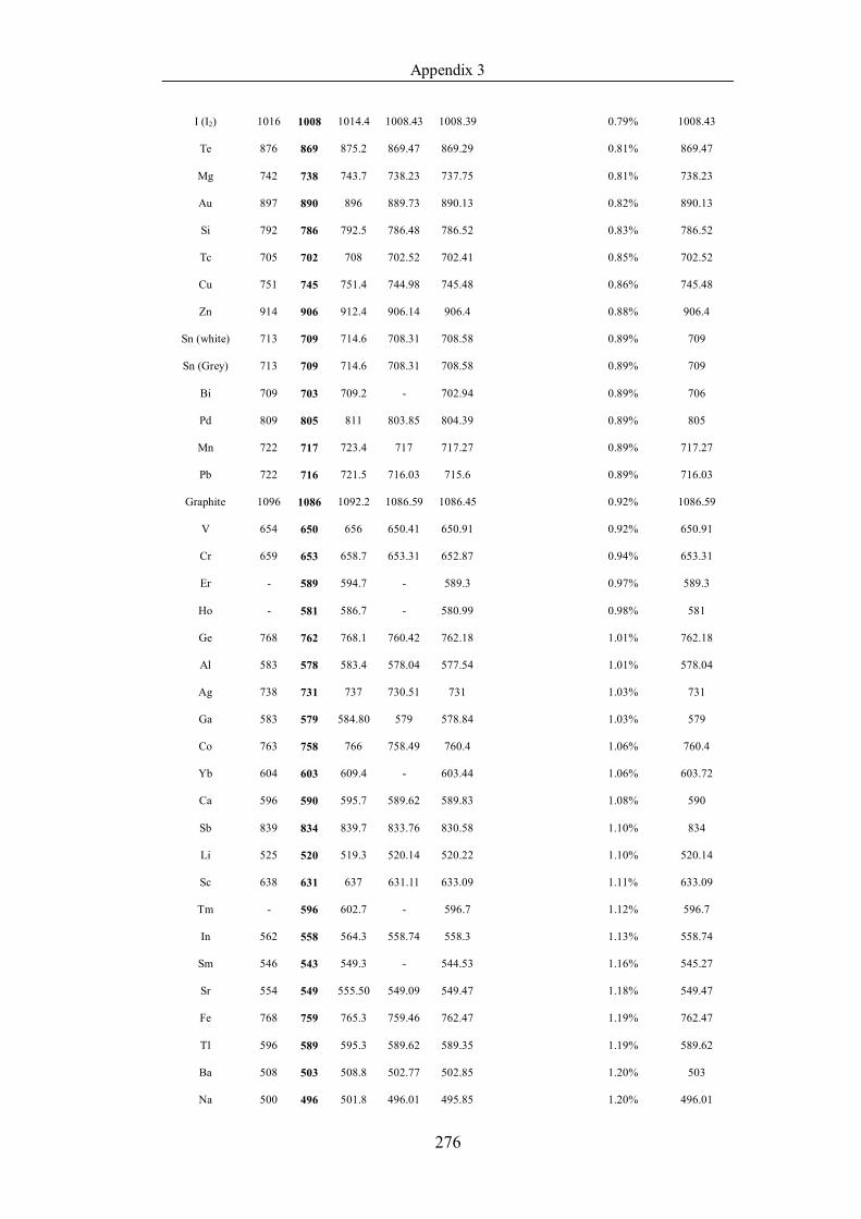
Appendix 3
276
I (I2) 1016 1008 1014.4 1008.43 1008.39 0.79% 1008.43
Te 876 869 875.2 869.47 869.29 0.81% 869.47
Mg 742 738 743.7 738.23 737.75 0.81% 738.23
Au 897 890 896 889.73 890.13 0.82% 890.13
Si 792 786 792.5 786.48 786.52 0.83% 786.52
Tc 705 702 708 702.52 702.41 0.85% 702.52
Cu 751 745 751.4 744.98 745.48 0.86% 745.48
Zn 914 906 912.4 906.14 906.4 0.88% 906.4
Sn (white) 713 709 714.6 708.31 708.58 0.89% 709
Sn (Grey) 713 709 714.6 708.31 708.58 0.89% 709
Bi 709 703 709.2 - 702.94 0.89% 706
Pd 809 805 811 803.85 804.39 0.89% 805
Mn 722 717 723.4 717 717.27 0.89% 717.27
Pb 722 716 721.5 716.03 715.6 0.89% 716.03
Graphite 1096 1086 1092.2 1086.59 1086.45 0.92% 1086.59
V 654 650 656 650.41 650.91 0.92% 650.91
Cr 659 653 658.7 653.31 652.87 0.94% 653.31
Er - 589 594.7 - 589.3 0.97% 589.3
Ho - 581 586.7 - 580.99 0.98% 581
Ge 768 762 768.1 760.42 762.18 1.01% 762.18
Al 583 578 583.4 578.04 577.54 1.01% 578.04
Ag 738 731 737 730.51 731 1.03% 731
Ga 583 579 584.80 579 578.84 1.03% 579
Co 763 758 766 758.49 760.4 1.06% 760.4
Yb 604 603 609.4 - 603.44 1.06% 603.72
Ca 596 590 595.7 589.62 589.83 1.08% 590
Sb 839 834 839.7 833.76 830.58 1.10% 834
Li 525 520 519.3 520.14 520.22 1.10% 520.14
Sc 638 631 637 631.11 633.09 1.11% 633.09
Tm - 596 602.7 - 596.7 1.12% 596.7
In 562 558 564.3 558.74 558.3 1.13% 558.74
Sm 546 543 549.3 - 544.53 1.16% 545.27
Sr 554 549 555.50 549.09 549.47 1.18% 549.47
Fe 768 759 765.3 759.46 762.47 1.19% 762.47
Tl 596 589 595.3 589.62 589.35 1.19% 589.62
Ba 508 503 508.8 502.77 502.85 1.20% 503
Na 500 496 501.8 496.01 495.85 1.20% 496.01
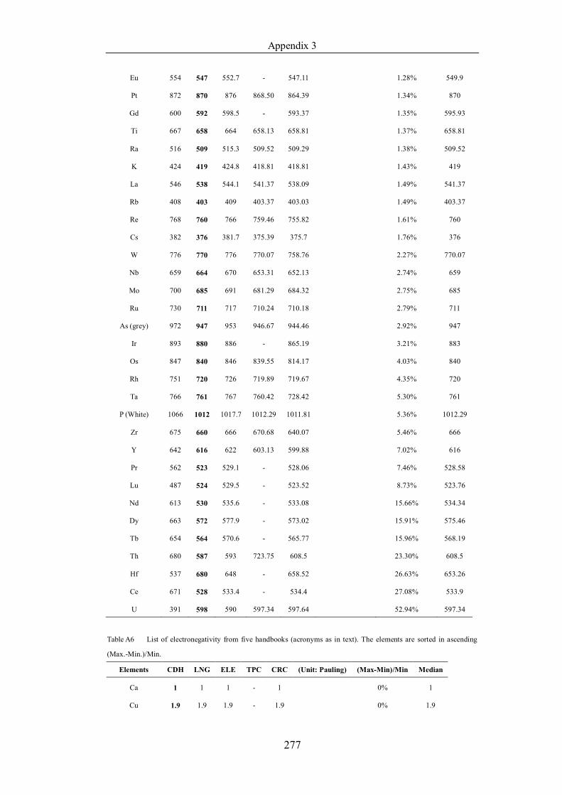
Appendix 3
277
Eu 554 547 552.7 - 547.11 1.28% 549.9
Pt 872 870 876 868.50 864.39 1.34% 870
Gd 600 592 598.5 - 593.37 1.35% 595.93
Ti 667 658 664 658.13 658.81 1.37% 658.81
Ra 516 509 515.3 509.52 509.29 1.38% 509.52
K 424 419 424.8 418.81 418.81 1.43% 419
La 546 538 544.1 541.37 538.09 1.49% 541.37
Rb 408 403 409 403.37 403.03 1.49% 403.37
Re 768 760 766 759.46 755.82 1.61% 760
Cs 382 376 381.7 375.39 375.7 1.76% 376
W 776 770 776 770.07 758.76 2.27% 770.07
Nb 659 664 670 653.31 652.13 2.74% 659
Mo 700 685 691 681.29 684.32 2.75% 685
Ru 730 711 717 710.24 710.18 2.79% 711
As (grey) 972 947 953 946.67 944.46 2.92% 947
Ir 893 880 886 - 865.19 3.21% 883
Os 847 840 846 839.55 814.17 4.03% 840
Rh 751 720 726 719.89 719.67 4.35% 720
Ta 766 761 767 760.42 728.42 5.30% 761
P (White) 1066 1012 1017.7 1012.29 1011.81 5.36% 1012.29
Zr 675 660 666 670.68 640.07 5.46% 666
Y 642 616 622 603.13 599.88 7.02% 616
Pr 562 523 529.1 - 528.06 7.46% 528.58
Lu 487 524 529.5 - 523.52 8.73% 523.76
Nd 613 530 535.6 - 533.08 15.66% 534.34
Dy 663 572 577.9 - 573.02 15.91% 575.46
Tb 654 564 570.6 - 565.77 15.96% 568.19
Th 680 587 593 723.75 608.5 23.30% 608.5
Hf 537 680 648 - 658.52 26.63% 653.26
Ce 671 528 533.4 - 534.4 27.08% 533.9
U 391 598 590 597.34 597.64 52.94% 597.34
Table A6 List of electronegativity from five handbooks (acronyms as in text). The elements are sorted in ascending
(Max.-Min.)/Min.
Elements CDH LNG ELE TPC CRC (Unit: Pauling) (Max-Min)/Min Median
Ca 1 1 1 - 1 0% 1
Cu 1.9 1.9 1.9 - 1.9 0% 1.9
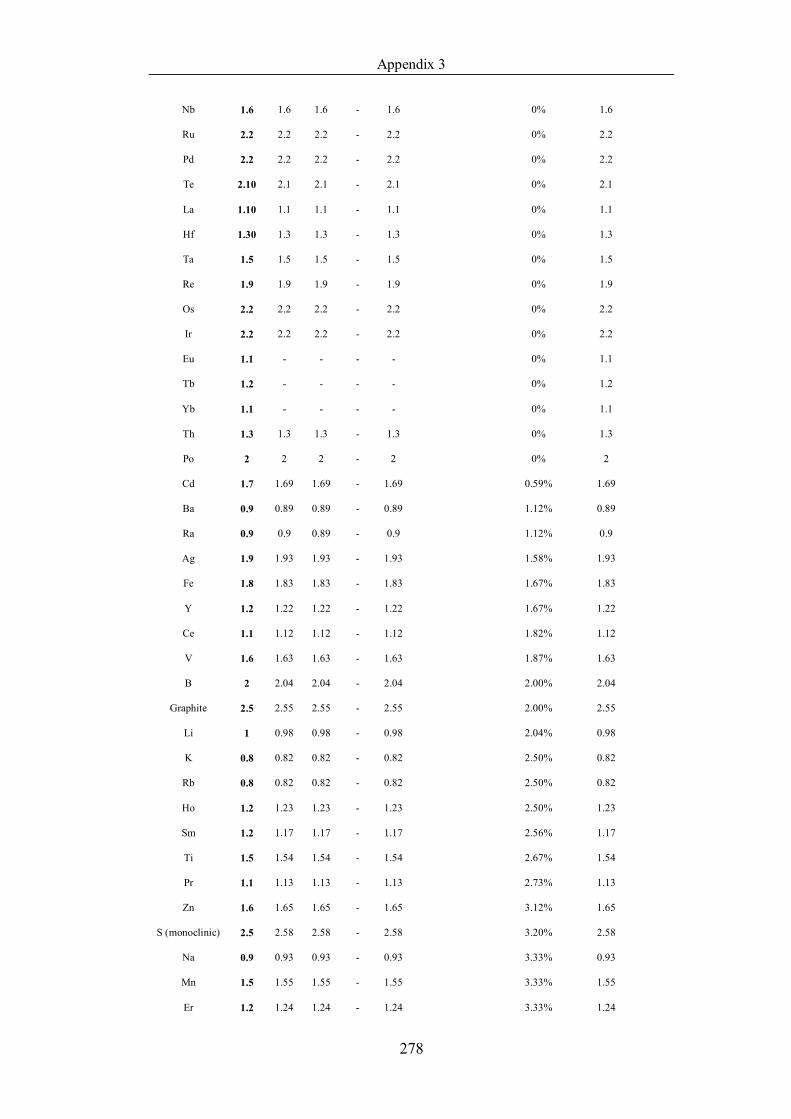
Appendix 3
278
Nb 1.6 1.6 1.6 - 1.6 0% 1.6
Ru 2.2 2.2 2.2 - 2.2 0% 2.2
Pd 2.2 2.2 2.2 - 2.2 0% 2.2
Te 2.10 2.1 2.1 - 2.1 0% 2.1
La 1.10 1.1 1.1 - 1.1 0% 1.1
Hf 1.30 1.3 1.3 - 1.3 0% 1.3
Ta 1.5 1.5 1.5 - 1.5 0% 1.5
Re 1.9 1.9 1.9 - 1.9 0% 1.9
Os 2.2 2.2 2.2 - 2.2 0% 2.2
Ir 2.2 2.2 2.2 - 2.2 0% 2.2
Eu 1.1 - - - - 0% 1.1
Tb 1.2 - - - - 0% 1.2
Yb 1.1 - - - - 0% 1.1
Th 1.3 1.3 1.3 - 1.3 0% 1.3
Po 2 2 2 - 2 0% 2
Cd 1.7 1.69 1.69 - 1.69 0.59% 1.69
Ba 0.9 0.89 0.89 - 0.89 1.12% 0.89
Ra 0.9 0.9 0.89 - 0.9 1.12% 0.9
Ag 1.9 1.93 1.93 - 1.93 1.58% 1.93
Fe 1.8 1.83 1.83 - 1.83 1.67% 1.83
Y 1.2 1.22 1.22 - 1.22 1.67% 1.22
Ce 1.1 1.12 1.12 - 1.12 1.82% 1.12
V 1.6 1.63 1.63 - 1.63 1.87% 1.63
B 2 2.04 2.04 - 2.04 2.00% 2.04
Graphite 2.5 2.55 2.55 - 2.55 2.00% 2.55
Li 1 0.98 0.98 - 0.98 2.04% 0.98
K 0.8 0.82 0.82 - 0.82 2.50% 0.82
Rb 0.8 0.82 0.82 - 0.82 2.50% 0.82
Ho 1.2 1.23 1.23 - 1.23 2.50% 1.23
Sm 1.2 1.17 1.17 - 1.17 2.56% 1.17
Ti 1.5 1.54 1.54 - 1.54 2.67% 1.54
Pr 1.1 1.13 1.13 - 1.13 2.73% 1.13
Zn 1.6 1.65 1.65 - 1.65 3.12% 1.65
S (monoclinic) 2.5 2.58 2.58 - 2.58 3.20% 2.58
Na 0.9 0.93 0.93 - 0.93 3.33% 0.93
Mn 1.5 1.55 1.55 - 1.55 3.33% 1.55
Er 1.2 1.24 1.24 - 1.24 3.33% 1.24
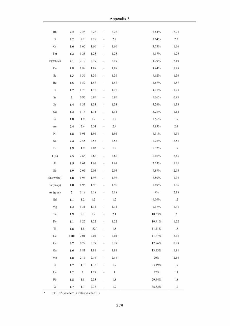
Appendix 3
279
Rh 2.2 2.28 2.28 - 2.28 3.64% 2.28
Pt 2.2 2.2 2.28 - 2.2 3.64% 2.2
Cr 1.6 1.66 1.66 - 1.66 3.75% 1.66
Tm 1.2 1.25 1.25 - 1.25 4.17% 1.25
P (White) 2.1 2.19 2.19 - 2.19 4.29% 2.19
Co 1.8 1.88 1.88 - 1.88 4.44% 1.88
Sc 1.3 1.36 1.36 - 1.36 4.62% 1.36
Be 1.5 1.57 1.57 - 1.57 4.67% 1.57
In 1.7 1.78 1.78 - 1.78 4.71% 1.78
Sr 1 0.95 0.95 - 0.95 5.26% 0.95
Zr 1.4 1.33 1.33 - 1.33 5.26% 1.33
Nd 1.2 1.14 1.14 - 1.14 5.26% 1.14
Si 1.8 1.9 1.9 - 1.9 5.56% 1.9
Au 2.4 2.4 2.54 - 2.4 5.83% 2.4
Ni 1.8 1.91 1.91 - 1.91 6.11% 1.91
Se 2.4 2.55 2.55 - 2.55 6.25% 2.55
Bi 1.9 1.9 2.02 - 1.9 6.32% 1.9
I (I2) 2.5 2.66 2.66 - 2.66 6.40% 2.66
Al 1.5 1.61 1.61 - 1.61 7.33% 1.61
Sb 1.9 2.05 2.05 - 2.05 7.89% 2.05
Sn (white) 1.8 1.96 1.96 - 1.96 8.89% 1.96
Sn (Grey) 1.8 1.96 1.96 - 1.96 8.89% 1.96
As (grey) 2 2.18 2.18 - 2.18 9% 2.18
Gd 1.1 1.2 1.2 - 1.2 9.09% 1.2
Mg 1.2 1.31 1.31 - 1.31 9.17% 1.31
Tc 1.9 2.1 1.9 - 2.1 10.53% 2
Dy 1.1 1.22 1.22 - 1.22 10.91% 1.22
Tl 1.8 1.8 1.62* - 1.8 11.11% 1.8
Ge 1.80 2.01 2.01 - 2.01 11.67% 2.01
Cs 0.7 0.79 0.79 - 0.79 12.86% 0.79
Ga 1.6 1.81 1.81 - 1.81 13.13% 1.81
Mo 1.8 2.16 2.16 - 2.16 20% 2.16
U 1.7 1.7 1.38 - 1.7 23.19% 1.7
Lu 1.2 1 1.27 - 1 27% 1.1
Pb 1.8 1.8 2.33 - 1.8 29.44% 1.8
W 1.7 1.7 2.36 - 1.7 38.82% 1.7
* Tl: 1.62 (valence: I), 2.04 (valence: II)
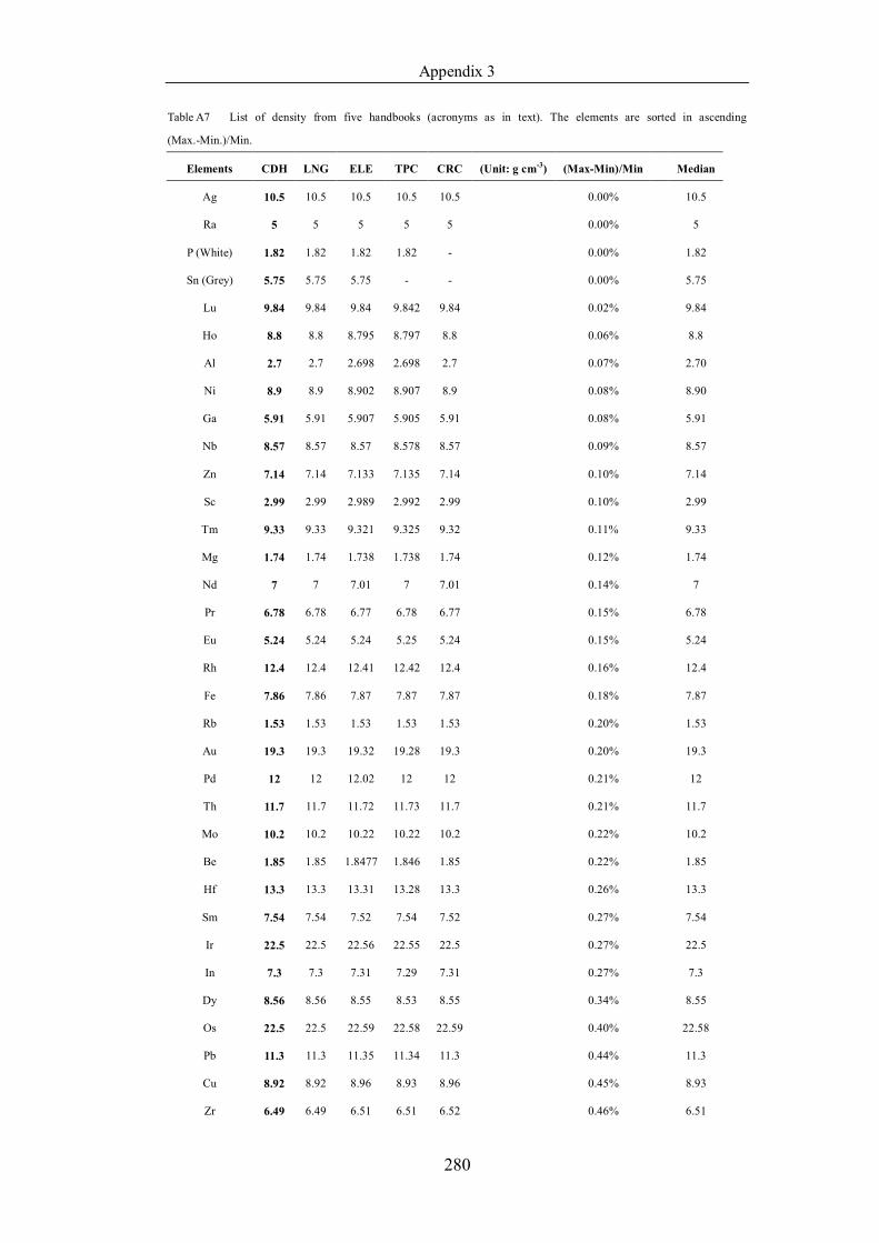
Appendix 3
280
Table A7 List of density from five handbooks (acronyms as in text). The elements are sorted in ascending
(Max.-Min.)/Min.
Elements CDH LNG ELE TPC CRC (Unit: g cm-3) (Max-Min)/Min Median
Ag 10.5 10.5 10.5 10.5 10.5 0.00% 10.5
Ra 5 5 5 5 5 0.00% 5
P (White) 1.82 1.82 1.82 1.82 - 0.00% 1.82
Sn (Grey) 5.75 5.75 5.75 - - 0.00% 5.75
Lu 9.84 9.84 9.84 9.842 9.84 0.02% 9.84
Ho 8.8 8.8 8.795 8.797 8.8 0.06% 8.8
Al 2.7 2.7 2.698 2.698 2.7 0.07% 2.70
Ni 8.9 8.9 8.902 8.907 8.9 0.08% 8.90
Ga 5.91 5.91 5.907 5.905 5.91 0.08% 5.91
Nb 8.57 8.57 8.57 8.578 8.57 0.09% 8.57
Zn 7.14 7.14 7.133 7.135 7.14 0.10% 7.14
Sc 2.99 2.99 2.989 2.992 2.99 0.10% 2.99
Tm 9.33 9.33 9.321 9.325 9.32 0.11% 9.33
Mg 1.74 1.74 1.738 1.738 1.74 0.12% 1.74
Nd 7 7 7.01 7 7.01 0.14% 7
Pr 6.78 6.78 6.77 6.78 6.77 0.15% 6.78
Eu 5.24 5.24 5.24 5.25 5.24 0.15% 5.24
Rh 12.4 12.4 12.41 12.42 12.4 0.16% 12.4
Fe 7.86 7.86 7.87 7.87 7.87 0.18% 7.87
Rb 1.53 1.53 1.53 1.53 1.53 0.20% 1.53
Au 19.3 19.3 19.32 19.28 19.3 0.20% 19.3
Pd 12 12 12.02 12 12 0.21% 12
Th 11.7 11.7 11.72 11.73 11.7 0.21% 11.7
Mo 10.2 10.2 10.22 10.22 10.2 0.22% 10.2
Be 1.85 1.85 1.8477 1.846 1.85 0.22% 1.85
Hf 13.3 13.3 13.31 13.28 13.3 0.26% 13.3
Sm 7.54 7.54 7.52 7.54 7.52 0.27% 7.54
Ir 22.5 22.5 22.56 22.55 22.5 0.27% 22.5
In 7.3 7.3 7.31 7.29 7.31 0.27% 7.3
Dy 8.56 8.56 8.55 8.53 8.55 0.34% 8.55
Os 22.5 22.5 22.59 22.58 22.59 0.40% 22.58
Pb 11.3 11.3 11.35 11.34 11.3 0.44% 11.3
Cu 8.92 8.92 8.96 8.93 8.96 0.45% 8.93
Zr 6.49 6.49 6.51 6.51 6.52 0.46% 6.51

Appendix 3
281
I (I2) 4.93 4.93 4.93 4.95 - 0.47% 4.93
Pt 21.4 21.4 21.45 21.45 21.5 0.47% 21.45
Tb 8.27 8.27 8.23 8.27 8.23 0.50% 8.27
Na 0.97 0.97 0.971 0.966 0.97 0.52% 0.97
Bi 9.8 9.8 9.75 9.8 9.79 0.57% 9.8
Cd 8.64 8.64 8.65 8.65 8.69 0.58% 8.65
Tl 11.8 11.8 11.85 11.87 11.8 0.60% 11.8
Cr 7.19 7.19 7.19 7.19 7.15 0.62% 7.19
Sn (white) 7.28 7.28 7.31 7.29 7.26 0.69% 7.28
Ti 4.54 4.54 4.54 4.51 4.51 0.71% 4.54
Graphite 2.25 2.25 2.26 2.27 - 0.71% 2.26
La 6.19 6.19 6.15 6.17 6.15 0.73% 6.17
Li 0.53 0.53 0.53 0.53 0.53 0.75% 0.53
W 19.4 19.4 19.3 19.25 19.3 0.76% 19.3
U 19.1 19.1 18.95 19.05 19.1 0.79% 19.1
Gd 7.95 7.95 7.9 7.87 7.9 1.02% 7.9
Ce 6.78 6.78 6.77* 6.71 6.77 1.03% 6.77
Sb 6.62 6.62 6.69 6.69 6.68 1.09% 6.68
Co 8.9 8.9 8.9 8.8 8.86 1.14% 8.9
Yb 6.98 6.98 6.97 6.97 6.9 1.16% 6.97
Er 9.16 9.16 9.07 9.04 9.07 1.28% 9.07
Ca 1.54 1.54 1.55 1.53 1.54 1.31% 1.54
Ta 16.6 16.6 16.65 16.67 16.4 1.65% 16.6
Po 9.4 9.4 9.32 9.4 9.2 2.17% 9.4
Ru 12.3 12.3 12.37 12.36 12.1 2.23% 12.3
V 5.96 5.96 6.11 6.09 6 2.52% 6
Re 20.5 20.5 21.02 21.02 20.8 2.55% 20.8
Cs 1.9 1.9 1.87 1.9 1.93 3.04% 1.9
Y 4.34 4.34 4.47 4.48 4.47 3.11% 4.47
Ba 3.51 3.51 3.59 3.59 3.62 3.13% 3.59
K 0.86 0.86 0.86 0.86 0.89 3.49% 0.86
Mn 7.2 7.2 7.44 7.47 7.3 3.79% 7.3
Sr 2.62 2.62 2.54 2.58 2.64 3.94% 2.62
Tc 11.5 11.5 11.5 11.5 11 4.55% 11.5
Ge 5.35 5.35 5.32 5.32 5.6** 5.20% 5.35
S (monoclinic) 1.96 1.96 1.96 - 1.82** 7.75% 1.96
Te 6.25 6.25 6.24 6.25 5.7** 9.65% 6.25
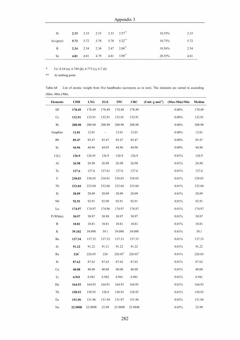
Appendix 3
282
Si 2.33 2.33 2.33 2.33 2.57** 10.35% 2.33
As (grey) 5.72 5.72 5.78 5.78 5.22** 10.73% 5.72
B 2.34 2.34 2.34 2.47 2.08** 18.56% 2.34
Se 4.81 4.81 4.79 4.81 3.99** 20.55% 4.81
* Ce: 8.24 (α), 6.749 (β), 6.773 (γ), 6.7 (δ)
** At melting point
Table A8 List of atomic weight from five handbooks (acronyms as in text). The elements are sorted in ascending
(Max.-Min.)/Min.
Elements CDH LNG ELE TPC CRC (Unit: g mol-1) (Max-Min)/Min Median
Hf 178.49 178.49 178.49 178.49 178.49 0.00% 178.49
Cs 132.91 132.91 132.91 132.91 132.91 0.00% 132.91
Bi 208.98 208.98 208.98 208.98 208.98 0.00% 208.98
Graphite 12.01 12.01 - 12.01 12.01 0.00% 12.01
Rb 85.47 85.47 85.47 85.47 85.47 0.00% 85.47
Sc 44.96 44.96 44.95 44.96 44.96 0.00% 44.96
I (I2) 126.9 126.91 126.9 126.9 126.9 0.01% 126.9
Al 26.98 26.98 26.98 26.98 26.98 0.01% 26.98
Te 127.6 127.6 127.61 127.6 127.6 0.01% 127.6
U 238.03 238.03 238.01 238.03 238.03 0.01% 238.03
Th 232.04 232.04 232.06 232.04 232.04 0.01% 232.04
Si 28.09 28.09 28.09 28.09 28.09 0.01% 28.09
Nb 92.91 92.91 92.90 92.91 92.91 0.01% 92.91
Lu 174.97 174.97 174.96 174.97 174.97 0.01% 174.97
P (White) 30.97 30.97 30.98 30.97 30.97 0.01% 30.97
B 10.81 10.81 10.81 10.81 10.81 0.01% 10.81
K 39.102 39.098 39.1 39.098 39.098 0.01% 39.1
Ba 137.34 137.33 137.33 137.33 137.33 0.01% 137.33
Zr 91.22 91.22 91.21 91.22 91.22 0.01% 91.22
Ra 226* 226.03 226 226.03* 226.03* 0.01% 226.03
Sr 87.62 87.62 87.63 87.62 87.62 0.01% 87.62
Ca 40.08 40.08 40.08 40.08 40.08 0.01% 40.08
Li 6.941 6.941 6.942 6.941 6.941 0.01% 6.941
Ho 164.93 164.93 164.91 164.93 164.93 0.01% 164.93
Tb 158.93 158.93 158.9 158.93 158.93 0.01% 158.93
Eu 151.96 151.96 151.94 151.97 151.96 0.02% 151.96
Na 22.9898 22.9898 22.99 22.9898 22.9898 0.02% 22.99
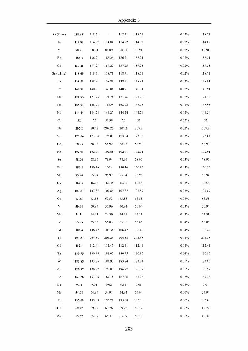
Appendix 3
283
Sn (Grey) 118.69* 118.71 - 118.71 118.71 0.02% 118.71
In 114.82 114.82 114.84 114.82 114.82 0.02% 114.82
Y 88.91 88.91 88.89 88.91 88.91 0.02% 88.91
Re 186.2 186.21 186.24 186.21 186.21 0.02% 186.21
Gd 157.25 157.25 157.22 157.25 157.25 0.02% 157.25
Sn (white) 118.69 118.71 118.71 118.71 118.71 0.02% 118.71
La 138.91 138.91 138.88 138.91 138.91 0.02% 138.91
Pr 140.91 140.91 140.88 140.91 140.91 0.02% 140.91
Sb 121.75 121.75 121.78 121.76 121.76 0.02% 121.76
Tm 168.93 168.93 168.9 168.93 168.93 0.02% 168.93
Nd 144.24 144.24 144.27 144.24 144.24 0.02% 144.24
Cr 52 52 51.98 52 52 0.02% 52
Pb 207.2 207.2 207.25 207.2 207.2 0.02% 207.2
Yb 173.04 173.04 173.01 173.04 173.05 0.03% 173.04
Co 58.93 58.93 58.92 58.93 58.93 0.03% 58.93
Rh 102.91 102.91 102.88 102.91 102.91 0.03% 102.91
Se 78.96 78.96 78.94 78.96 78.96 0.03% 78.96
Sm 150.4 150.36 150.4 150.36 150.36 0.03% 150.36
Mo 95.94 95.94 95.97 95.94 95.96 0.03% 95.94
Dy 162.5 162.5 162.45 162.5 162.5 0.03% 162.5
Ag 107.87 107.87 107.84 107.87 107.87 0.03% 107.87
Cu 63.55 63.55 63.53 63.55 63.55 0.03% 63.55
V 50.94 50.94 50.96 50.94 50.94 0.03% 50.94
Mg 24.31 24.31 24.30 24.31 24.31 0.03% 24.31
Fe 55.85 55.85 55.83 55.85 55.85 0.04% 55.85
Pd 106.4 106.42 106.38 106.42 106.42 0.04% 106.42
Tl 204.37 204.38 204.29 204.38 204.38 0.04% 204.38
Cd 112.4 112.41 112.45 112.41 112.41 0.04% 112.41
Ta 180.95 180.95 181.03 180.95 180.95 0.04% 180.95
W 183.85 183.85 183.93 183.84 183.84 0.05% 183.85
Au 196.97 196.97 196.87 196.97 196.97 0.05% 196.97
Er 167.26 167.26 167.18 167.26 167.26 0.05% 167.26
Be 9.01 9.01 9.02 9.01 9.01 0.05% 9.01
Mn 54.94 54.94 54.91 54.94 54.94 0.06% 54.94
Pt 195.09 195.08 195.20 195.08 195.08 0.06% 195.08
Ga 69.72 69.72 69.76 69.72 69.72 0.06% 69.72
Zn 65.37 65.39 65.41 65.39 65.38 0.06% 65.39
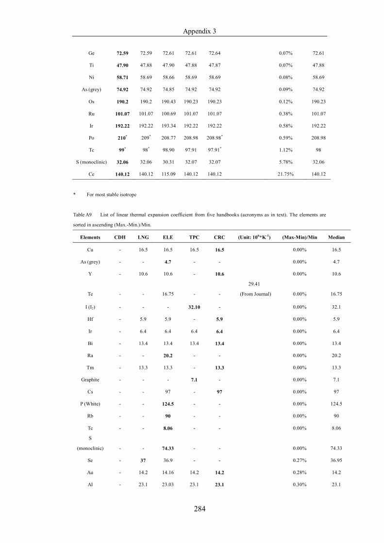
Appendix 3
284
Ge 72.59 72.59 72.61 72.61 72.64 0.07% 72.61
Ti 47.90 47.88 47.90 47.88 47.87 0.07% 47.88
Ni 58.71 58.69 58.66 58.69 58.69 0.08% 58.69
As (grey) 74.92 74.92 74.85 74.92 74.92 0.09% 74.92
Os 190.2 190.2 190.43 190.23 190.23 0.12% 190.23
Ru 101.07 101.07 100.69 101.07 101.07 0.38% 101.07
Ir 192.22 192.22 193.34 192.22 192.22 0.58% 192.22
Po 210* 209* 208.77 208.98 208.98* 0.59% 208.98
Tc 99* 98* 98.90 97.91 97.91* 1.12% 98
S (monoclinic) 32.06 32.06 30.31 32.07 32.07 5.78% 32.06
Ce 140.12 140.12 115.09 140.12 140.12 21.75% 140.12
* For most stable isotrope
Table A9 List of linear thermal expansion coefficient from five handbooks (acronyms as in text). The elements are
sorted in ascending (Max.-Min.)/Min.
Elements CDH LNG ELE TPC CRC (Unit: 106*K-1) (Max-Min)/Min Median
Cu - 16.5 16.5 16.5 16.5 0.00% 16.5
As (grey) - - 4.7 - - 0.00% 4.7
Y - 10.6 10.6 - 10.6 0.00% 10.6
Te - - 16.75 - -
29.41
(From Journal) 0.00% 16.75
I (I2) - - - 32.10 - 0.00% 32.1
Hf - 5.9 5.9 - 5.9 0.00% 5.9
Ir - 6.4 6.4 6.4 6.4 0.00% 6.4
Bi - 13.4 13.4 13.4 13.4 0.00% 13.4
Ra - - 20.2 - - 0.00% 20.2
Tm - 13.3 13.3 - 13.3 0.00% 13.3
Graphite - - - 7.1 - 0.00% 7.1
Cs - - 97 - 97 0.00% 97
P (White) - - 124.5 - - 0.00% 124.5
Rb - - 90 - - 0.00% 90
Tc - - 8.06 - - 0.00% 8.06
S
(monoclinic) - - 74.33 - - 0.00% 74.33
Se - 37 36.9 - - 0.27% 36.95
Au - 14.2 14.16 14.2 14.2 0.28% 14.2
Al - 23.1 23.03 23.1 23.1 0.30% 23.1
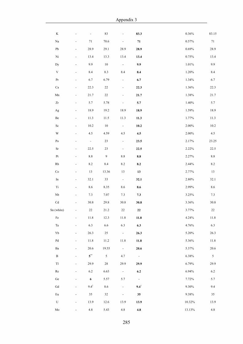
Appendix 3
285
K - - 83 - 83.3 0.36% 83.15
Na - 71 70.6 - 71 0.57% 71
Pb - 28.9 29.1 28.9 28.9 0.69% 28.9
Ni - 13.4 13.3 13.4 13.4 0.75% 13.4
Dy - 9.9 10 - 9.9 1.01% 9.9
V - 8.4 8.3 8.4 8.4 1.20% 8.4
Pr - 6.7 6.79 - 6.7 1.34% 6.7
Ca - 22.3 22 - 22.3 1.36% 22.3
Mn - 21.7 22 - 21.7 1.38% 21.7
Zr - 5.7 5.78 - 5.7 1.40% 5.7
Ag - 18.9 19.2 18.9 18.9 1.59% 18.9
Be - 11.3 11.5 11.3 11.3 1.77% 11.3
Sc - 10.2 10 - 10.2 2.00% 10.2
W - 4.5 4.59 4.5 4.5 2.00% 4.5
Po - - 23 - 23.5 2.17% 23.25
Sr - 22.5 23 - 22.5 2.22% 22.5
Pt - 8.8 9 8.8 8.8 2.27% 8.8
Rh - 8.2 8.4 8.2 8.2 2.44% 8.2
Co - 13 13.36 13 13 2.77% 13
In - 32.1 33 - 32.1 2.80% 32.1
Ti - 8.6 8.35 8.6 8.6 2.99% 8.6
Nb - 7.3 7.07 7.3 7.3 3.25% 7.3
Cd - 30.8 29.8 30.8 30.8 3.36% 30.8
Sn (white) - 22 21.2 22 22 3.77% 22
Fe - 11.8 12.3 11.8 11.8 4.24% 11.8
Ta - 6.3 6.6 6.3 6.3 4.76% 6.3
Yb - 26.3 25 - 26.3 5.20% 26.3
Pd - 11.8 11.2 11.8 11.8 5.36% 11.8
Ba - 20.6 19.55 - 20.6 5.37% 20.6
B - 5** 5 4.7 - 6.38% 5
Tl - 29.9 28 29.9 29.9 6.79% 29.9
Re - 6.2 6.63 - 6.2 6.94% 6.2
Ge - 6 5.57 5.7 - 7.72% 5.7
Gd - 9.4↑ 8.6 - 9.4↑ 9.30% 9.4
Eu - 35 32 - 35 9.38% 35
U - 13.9 12.6 13.9 13.9 10.32% 13.9
Mo - 4.8 5.43 4.8 4.8 13.13% 4.8
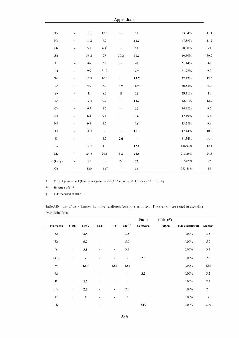
Appendix 3
286
Th - 11.1 12.5 - 11 13.64% 11.1
Ho - 11.2 9.5 - 11.2 17.89% 11.2
Os - 5.1 4.3* - 5.1 18.60% 5.1
Zn - 30.2 25 30.2 30.2 20.80% 30.2
Li - 46 56 - 46 21.74% 46
Lu - 9.9 8.12 - 9.9 21.92% 9.9
Sm - 12.7 10.4 - 12.7 22.12% 12.7
Cr - 4.9 6.2 4.9 4.9 26.53% 4.9
Sb - 11 8.5 11 11 29.41% 11
Er - 12.2 9.2 - 12.2 32.61% 12.2
Ce - 6.3 8.5 - 6.3 34.92% 6.3
Ru - 6.4 9.1 - 6.4 42.19% 6.4
Nd - 9.6 6.7 - 9.6 43.28% 9.6
Tb - 10.3 7 - 10.3 47.14% 10.3
Si - - 4.2 2.6 - 61.54% 3.4
La - 12.1 4.9 - 12.1 146.94% 12.1
Mg - 24.8 26.1 8.2 24.8 218.29% 24.8
Sn (Grey) - 22 5.3 22 22 315.09% 22
Ga - 120 11.5* - 18 943.48% 18
* Os: 4.3 (a axis), 6.1 (b axis), 6.8 (c axis); Ga: 11.5 (a axis), 31.5 (b axis), 16.5 (c axis)
** B: range of 5~7
↑ Gd: recorded at 100 ºC
Table A10 List of work function from five handbooks (acronyms as in text). The elements are sorted in ascending
(Max.-Min.)/Min.
Elements CDH LNG ELE TPC CRC**
Ptable
Software
(Unit: eV)
Polycr. (Max-Min)/Min Median
Sc - 3.5 - - 3.5 0.00% 3.5
Se - 5.9 - - 5.9 0.00% 5.9
Y - 3.1 - - 3.1 0.00% 3.1
I (I2) - - - - - 2.8 0.00% 2.8
W - 4.55 - 4.55 4.55 0.00% 4.55
Ra - - - - - 3.2 0.00% 3.2
Pr - 2.7 - - - 0.00% 2.7
Eu - 2.5 - - 2.5 0.00% 2.5
Tb - 3 - - 3 0.00% 3
Dy - - - - - 3.09 0.00% 3.09
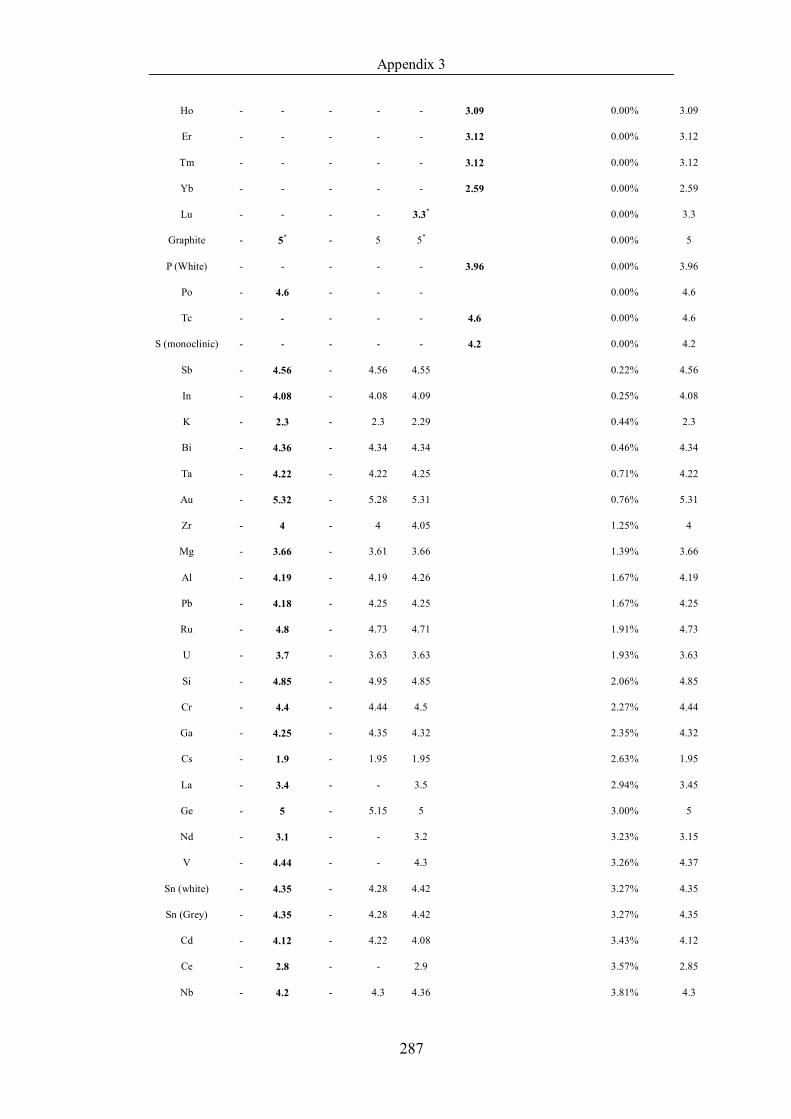
Appendix 3
287
Ho - - - - - 3.09 0.00% 3.09
Er - - - - - 3.12 0.00% 3.12
Tm - - - - - 3.12 0.00% 3.12
Yb - - - - - 2.59 0.00% 2.59
Lu - - - - 3.3* 0.00% 3.3
Graphite - 5* - 5 5* 0.00% 5
P (White) - - - - - 3.96 0.00% 3.96
Po - 4.6 - - - 0.00% 4.6
Tc - - - - - 4.6 0.00% 4.6
S (monoclinic) - - - - - 4.2 0.00% 4.2
Sb - 4.56 - 4.56 4.55 0.22% 4.56
In - 4.08 - 4.08 4.09 0.25% 4.08
K - 2.3 - 2.3 2.29 0.44% 2.3
Bi - 4.36 - 4.34 4.34 0.46% 4.34
Ta - 4.22 - 4.22 4.25 0.71% 4.22
Au - 5.32 - 5.28 5.31 0.76% 5.31
Zr - 4 - 4 4.05 1.25% 4
Mg - 3.66 - 3.61 3.66 1.39% 3.66
Al - 4.19 - 4.19 4.26 1.67% 4.19
Pb - 4.18 - 4.25 4.25 1.67% 4.25
Ru - 4.8 - 4.73 4.71 1.91% 4.73
U - 3.7 - 3.63 3.63 1.93% 3.63
Si - 4.85 - 4.95 4.85 2.06% 4.85
Cr - 4.4 - 4.44 4.5 2.27% 4.44
Ga - 4.25 - 4.35 4.32 2.35% 4.32
Cs - 1.9 - 1.95 1.95 2.63% 1.95
La - 3.4 - - 3.5 2.94% 3.45
Ge - 5 - 5.15 5 3.00% 5
Nd - 3.1 - - 3.2 3.23% 3.15
V - 4.44 - - 4.3 3.26% 4.37
Sn (white) - 4.35 - 4.28 4.42 3.27% 4.35
Sn (Grey) - 4.35 - 4.28 4.42 3.27% 4.35
Cd - 4.12 - 4.22 4.08 3.43% 4.12
Ce - 2.8 - - 2.9 3.57% 2.85
Nb - 4.2 - 4.3 4.36 3.81% 4.3
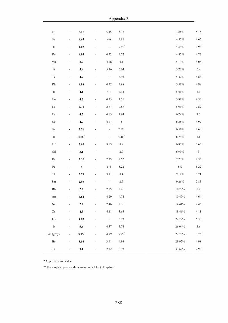
Appendix 3
288
Ni - 5.15 - 5.15 5.35 3.88% 5.15
Fe - 4.65 - 4.6 4.81 4.57% 4.65
Tl - 4.02 - - 3.84* 4.69% 3.93
Re - 4.95 - 4.72 4.72 4.87% 4.72
Mn - 3.9 - 4.08 4.1 5.13% 4.08
Pt - 5.4 - 5.36 5.64 5.22% 5.4
Te - 4.7 - - 4.95 5.32% 4.83
Rh - 4.98 - 4.72 4.98 5.51% 4.98
Ti - 4.1 - 4.1 4.33 5.61% 4.1
Mo - 4.3 - 4.33 4.55 5.81% 4.33
Ca - 2.71 - 2.87 2.87 5.90% 2.87
Cu - 4.7 - 4.65 4.94 6.24% 4.7
Co - 4.7 - 4.97 5 6.38% 4.97
Sr - 2.76 - - 2.59* 6.56% 2.68
B - 4.75* - - 4.45* 6.74% 4.6
Hf - 3.65 - 3.65 3.9 6.85% 3.65
Gd - 3.1 - - 2.9 6.90% 3
Ba - 2.35 - 2.35 2.52 7.23% 2.35
Pd - 5 - 5.4 5.22 8% 5.22
Th - 3.71 - 3.71 3.4 9.12% 3.71
Sm - 2.95 - - 2.7 9.26% 2.83
Rb - 2.2 - 2.05 2.26 10.29% 2.2
Ag - 4.64 - 4.29 4.74 10.49% 4.64
Na - 2.7 - 2.46 2.36 14.41% 2.46
Zn - 4.3 - 4.11 3.63 18.46% 4.11
Os - 4.83 - - 5.93 22.77% 5.38
Ir - 5.6 - 4.57 5.76 26.04% 5.6
As (grey) - 3.75* - 4.79 3.75* 27.73% 3.75
Be - 5.08 - 3.91 4.98 29.92% 4.98
Li - 3.1 - 2.32 2.93 33.62% 2.93
* Approximation value
** For single crystals, values are recorded for (111) plane
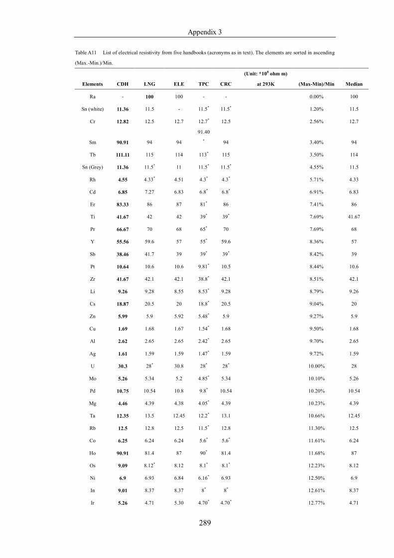
Appendix 3
289
Table A11 List of electrical resistivity from five handbooks (acronyms as in text). The elements are sorted in ascending
(Max.-Min.)/Min.
Elements CDH LNG ELE TPC CRC
(Unit: *108 ohm m)
at 293K (Max-Min)/Min Median
Ra - 100 100 - - 0.00% 100
Sn (white) 11.36 11.5 - 11.5* 11.5* 1.20% 11.5
Cr 12.82 12.5 12.7 12.7* 12.5 2.56% 12.7
Sm 90.91 94 94
91.40* 94 3.40% 94
Tb 111.11 115 114 113* 115 3.50% 114
Sn (Grey) 11.36 11.5* 11 11.5* 11.5* 4.55% 11.5
Rh 4.55 4.33* 4.51 4.3* 4.3* 5.71% 4.33
Cd 6.85 7.27 6.83 6.8* 6.8* 6.91% 6.83
Er 83.33 86 87 81* 86 7.41% 86
Ti 41.67 42 42 39* 39* 7.69% 41.67
Pr 66.67 70 68 65* 70 7.69% 68
Y 55.56 59.6 57 55* 59.6 8.36% 57
Sb 38.46 41.7 39 39* 39* 8.42% 39
Pt 10.64 10.6 10.6 9.81* 10.5 8.44% 10.6
Zr 41.67 42.1 42.1 38.8* 42.1 8.51% 42.1
Li 9.26 9.28 8.55 8.53* 9.28 8.79% 9.26
Cs 18.87 20.5 20 18.8* 20.5 9.04% 20
Zn 5.99 5.9 5.92 5.48* 5.9 9.27% 5.9
Cu 1.69 1.68 1.67 1.54* 1.68 9.50% 1.68
Al 2.62 2.65 2.65 2.42* 2.65 9.70% 2.65
Ag 1.61 1.59 1.59 1.47* 1.59 9.72% 1.59
U 30.3 28* 30.8 28* 28* 10.00% 28
Mo 5.26 5.34 5.2 4.85* 5.34 10.10% 5.26
Pd 10.75 10.54 10.8 9.8* 10.54 10.20% 10.54
Mg 4.46 4.39 4.38 4.05* 4.39 10.23% 4.39
Ta 12.35 13.5 12.45 12.2* 13.1 10.66% 12.45
Rb 12.5 12.8 12.5 11.5* 12.8 11.30% 12.5
Co 6.25 6.24 6.24 5.6* 5.6* 11.61% 6.24
Ho 90.91 81.4 87 90* 81.4 11.68% 87
Os 9.09 8.12* 8.12 8.1* 8.1* 12.23% 8.12
Ni 6.9 6.93 6.84 6.16* 6.93 12.50% 6.9
In 9.01 8.37 8.37 8* 8* 12.61% 8.37
Ir 5.26 4.71 5.30 4.70* 4.70* 12.77% 4.71
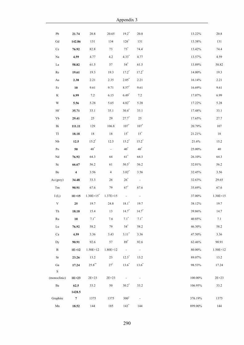
Appendix 3
290
Pb 21.74 20.8 20.65 19.2* 20.8 13.22% 20.8
Gd 142.86 131 134 126* 131 13.38% 131
Ce 76.92 82.8¦ 73 73* 74.4¦ 13.42% 74.4
Na 4.59 4.77 4.2 4.33* 4.77 13.57% 4.59
La 58.82 61.5 57 54* 61.5 13.89% 58.82
Re 19.61 19.3 19.3 17.2* 17.2* 14.00% 19.3
Au 2.38 2.21 2.35 2.05* 2.21 16.14% 2.21
Fe 10 9.61 9.71 8.57* 9.61 16.69% 9.61
K 6.99 7.2 6.15 6.49* 7.2 17.07% 6.99
W 5.56 5.28 5.65 4.82* 5.28 17.22% 5.28
Hf 35.71 33.1 35.1 30.4* 33.1 17.48% 33.1
Yb 29.41 25 29 27.7* 25 17.65% 27.7
Bi 111.11 129 106.8 107* 107* 20.79% 107
Tl 18.18 18 18 15* 15* 21.21% 18
Nb 12.5 15.2* 12.5 15.2* 15.2* 21.6% 15.2
Po 50 40* - 40* 40* 25.00% 40
Nd 76.92 64.3 64 61* 64.3 26.10% 64.3
Sc 66.67 56.2 61 50.5* 56.2 32.01% 56.2
Be 4 3.56 4 3.02* 3.56 32.45% 3.56
As (grey) 34.48 33.3 26 26* - 32.63% 29.65
Tm 90.91 67.6 79 67* 67.6 35.69% 67.6
I (I2) 1E+15 1.30E+15* 1.37E+15 - - 37.00% 1.30E+15
V 25 19.7 24.8 18.1* 19.7 38.12% 19.7
Th 18.18 15.4 13 14.7* 14.7* 39.86% 14.7
Ru 10 7.1* 7.6 7.1* 7.1* 40.85% 7.1
Lu 76.92 58.2 79 54* 58.2 46.30% 58.2
Ca 4.59 3.36 3.43 3.11* 3.36 47.50% 3.36
Dy 90.91 92.6 57 89* 92.6 62.46% 90.91
B 1E+12 1.50E+12 1.80E+12 - - 80.00% 1.50E+12
Sr 23.26 13.2 23 12.3* 13.2 89.07% 13.2
Ga 17.24 25.8** 27↑ 13.6* 13.6* 98.53% 17.24
S
(monoclinic) 1E+23 2E+23 2E+23 - - 100.00% 2E+23
Ba 62.5 33.2 50 30.2* 33.2 106.95% 33.2
Graphite
1428.5
7 1375 1375 300↕ - 376.19% 1375
Mn 18.52 144 185 143* 144 899.00% 144
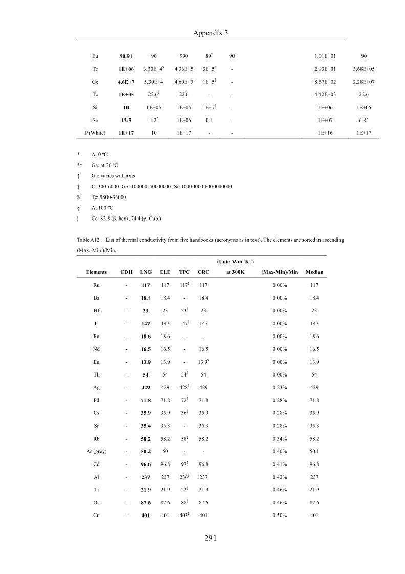
Appendix 3
291
Eu 90.91 90 990 89* 90 1.01E+01 90
Te 1E+06 3.30E+4$ 4.36E+5 3E+5$ - 2.93E+01 3.68E+05
Ge 4.6E+7 5.30E+4 4.60E+7 1E+5↕ - 8.67E+02 2.28E+07
Tc 1E+05 22.6§ 22.6 - - 4.42E+03 22.6
Si 10 1E+05 1E+05 1E+7↕ - 1E+06 1E+05
Se 12.5 1.2* 1E+06 0.1 - 1E+07 6.85
P (White) 1E+17 10 1E+17 - - 1E+16 1E+17
* At 0 ºC
** Ga: at 30 ºC
↑ Ga: varies with axis
↕ C: 300-6000; Ge: 100000-50000000; Si: 10000000-6000000000
$ Te: 5800-33000
§ At 100 ºC
¦ Ce: 82.8 (β, hex), 74.4 (γ, Cub.)
Table A12 List of thermal conductivity from five handbooks (acronyms as in text). The elements are sorted in ascending
(Max.-Min.)/Min.
Elements CDH LNG ELE TPC CRC
(Unit: Wm-1K-1)
at 300K (Max-Min)/Min Median
Ru - 117 117 117↕ 117 0.00% 117
Ba - 18.4 18.4 - 18.4 0.00% 18.4
Hf - 23 23 23↕ 23 0.00% 23
Ir - 147 147 147↕ 147 0.00% 147
Ra - 18.6 18.6 - - 0.00% 18.6
Nd - 16.5 16.5 - 16.5 0.00% 16.5
Eu - 13.9 13.9 - 13.9$ 0.00% 13.9
Th - 54 54 54↕ 54 0.00% 54
Ag - 429 429 428↕ 429 0.23% 429
Pd - 71.8 71.8 72↕ 71.8 0.28% 71.8
Cs - 35.9 35.9 36↕ 35.9 0.28% 35.9
Sr - 35.4 35.3 - 35.3 0.28% 35.3
Rb - 58.2 58.2 58↕ 58.2 0.34% 58.2
As (grey) - 50.2 50 - - 0.40% 50.1
Cd - 96.6 96.8 97↕ 96.8 0.41% 96.8
Al - 237 237 236↕ 237 0.42% 237
Ti - 21.9 21.9 22↕ 21.9 0.46% 21.9
Os - 87.6 87.6 88↕ 87.6 0.46% 87.6
Cu - 401 401 403↕ 401 0.50% 401
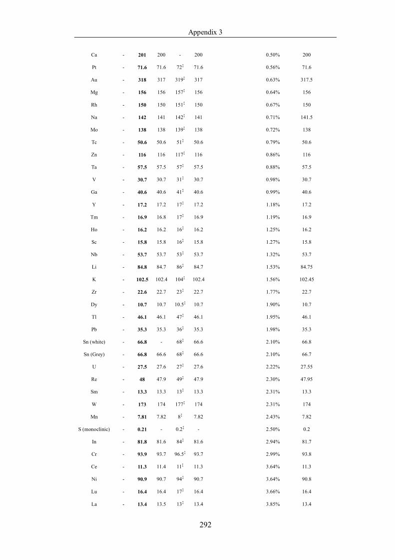
Appendix 3
292
Ca - 201 200 - 200 0.50% 200
Pt - 71.6 71.6 72↕ 71.6 0.56% 71.6
Au - 318 317 319↕ 317 0.63% 317.5
Mg - 156 156 157↕ 156 0.64% 156
Rh - 150 150 151↕ 150 0.67% 150
Na - 142 141 142↕ 141 0.71% 141.5
Mo - 138 138 139↕ 138 0.72% 138
Tc - 50.6 50.6 51↕ 50.6 0.79% 50.6
Zn - 116 116 117↕ 116 0.86% 116
Ta - 57.5 57.5 57↕ 57.5 0.88% 57.5
V - 30.7 30.7 31↕ 30.7 0.98% 30.7
Ga - 40.6 40.6 41↕ 40.6 0.99% 40.6
Y - 17.2 17.2 17↕ 17.2 1.18% 17.2
Tm - 16.9 16.8 17↕ 16.9 1.19% 16.9
Ho - 16.2 16.2 16↕ 16.2 1.25% 16.2
Sc - 15.8 15.8 16↕ 15.8 1.27% 15.8
Nb - 53.7 53.7 53↕ 53.7 1.32% 53.7
Li - 84.8 84.7 86↕ 84.7 1.53% 84.75
K - 102.5 102.4 104↕ 102.4 1.56% 102.45
Zr - 22.6 22.7 23↕ 22.7 1.77% 22.7
Dy - 10.7 10.7 10.5↕ 10.7 1.90% 10.7
Tl - 46.1 46.1 47↕ 46.1 1.95% 46.1
Pb - 35.3 35.3 36↕ 35.3 1.98% 35.3
Sn (white) - 66.8 - 68↕ 66.6 2.10% 66.8
Sn (Grey) - 66.8 66.6 68↕ 66.6 2.10% 66.7
U - 27.5 27.6 27↕ 27.6 2.22% 27.55
Re - 48 47.9 49↕ 47.9 2.30% 47.95
Sm - 13.3 13.3 13↕ 13.3 2.31% 13.3
W - 173 174 177↕ 174 2.31% 174
Mn - 7.81 7.82 8↕ 7.82 2.43% 7.82
S (monoclinic) - 0.21 - 0.2↕ - 2.50% 0.2
In - 81.8 81.6 84↕ 81.6 2.94% 81.7
Cr - 93.9 93.7 96.5↕ 93.7 2.99% 93.8
Ce - 11.3 11.4 11↕ 11.3 3.64% 11.3
Ni - 90.9 90.7 94↕ 90.7 3.64% 90.8
Lu - 16.4 16.4 17↕ 16.4 3.66% 16.4
La - 13.4 13.5 13↕ 13.4 3.85% 13.4
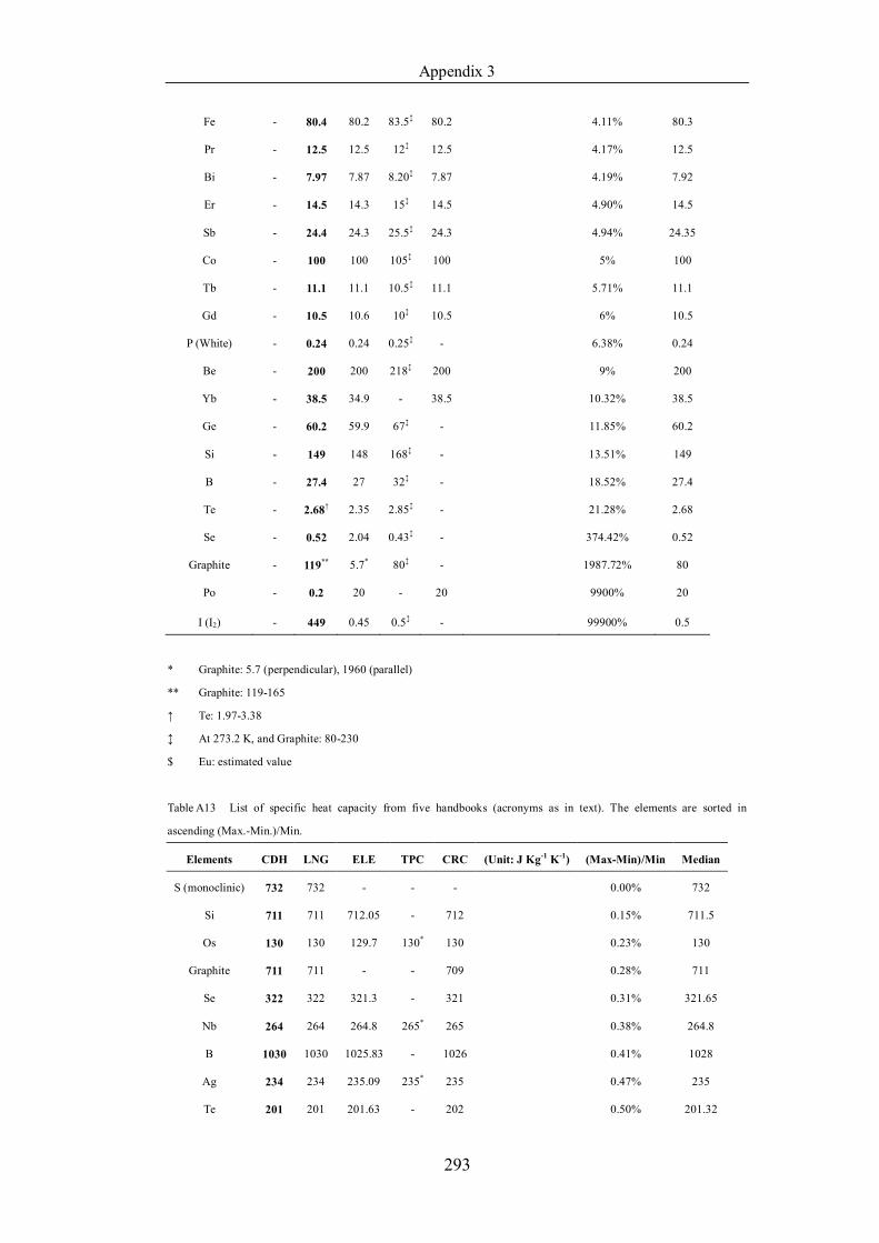
Appendix 3
293
Fe - 80.4 80.2 83.5↕ 80.2 4.11% 80.3
Pr - 12.5 12.5 12↕ 12.5 4.17% 12.5
Bi - 7.97 7.87 8.20↕ 7.87 4.19% 7.92
Er - 14.5 14.3 15↕ 14.5 4.90% 14.5
Sb - 24.4 24.3 25.5↕ 24.3 4.94% 24.35
Co - 100 100 105↕ 100 5% 100
Tb - 11.1 11.1 10.5↕ 11.1 5.71% 11.1
Gd - 10.5 10.6 10↕ 10.5 6% 10.5
P (White) - 0.24 0.24 0.25↕ - 6.38% 0.24
Be - 200 200 218↕ 200 9% 200
Yb - 38.5 34.9 - 38.5 10.32% 38.5
Ge - 60.2 59.9 67↕ - 11.85% 60.2
Si - 149 148 168↕ - 13.51% 149
B - 27.4 27 32↕ - 18.52% 27.4
Te - 2.68↑ 2.35 2.85↕ - 21.28% 2.68
Se - 0.52 2.04 0.43↕ - 374.42% 0.52
Graphite - 119** 5.7* 80↕ - 1987.72% 80
Po - 0.2 20 - 20 9900% 20
I (I2) - 449 0.45 0.5↕ - 99900% 0.5
* Graphite: 5.7 (perpendicular), 1960 (parallel)
** Graphite: 119-165
↑ Te: 1.97-3.38
↕ At 273.2 K, and Graphite: 80-230
$ Eu: estimated value
Table A13 List of specific heat capacity from five handbooks (acronyms as in text). The elements are sorted in
ascending (Max.-Min.)/Min.
Elements CDH LNG ELE TPC CRC (Unit: J Kg-1 K-1) (Max-Min)/Min Median
S (monoclinic) 732 732 - - - 0.00% 732
Si 711 711 712.05 - 712 0.15% 711.5
Os 130 130 129.7 130* 130 0.23% 130
Graphite 711 711 - - 709 0.28% 711
Se 322 322 321.3 - 321 0.31% 321.65
Nb 264 264 264.8 265* 265 0.38% 264.8
B 1030 1030 1025.83 - 1026 0.41% 1028
Ag 234 234 235.09 235* 235 0.47% 235
Te 201 201 201.63 - 202 0.50% 201.32
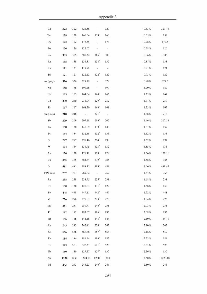
Appendix 3
294
Ge 322 322 321.56 - 320 0.63% 321.78
Tm 159 159 160.04 159* 160 0.65% 159
Dy 172 172 173.35 - 173 0.78% 172.5
Po 126 126 125.02 - - 0.78% 126
Zn 385 385 388.32 385* 388 0.86% 385
Re 138 138 136.81 138* 137 0.87% 138
Ra 121 121 119.91 - - 0.91% 121
Bi 121 121 122.12 122* 122 0.93% 122
As (grey) 326 326 329.19 - 329 0.98% 327.5
Nd 188 188 190.26 - 190 1.20% 189
Ho 163 163 164.64 164* 165 1.23% 164
Cd 230 230 231.04 229* 232 1.31% 230
Er 167 167 168.20 166* 168 1.33% 167
Sn (Grey) 218 218 - 221* - 1.38% 218
Sb 209 209 207.18 206* 207 1.46% 207.18
Ta 138 138 140.09 139* 140 1.51% 139
Pt 134 134 132.48 132* 133 1.52% 133
Y 297 297 298.46 294* 298 1.52% 297
W 134 134 131.95 133* 132 1.55% 133
Au 130 130 129.11 128* 129 1.56% 129.11
Cu 385 385 384.64 379* 385 1.58% 385
V 481 481 488.45 489* 489 1.66% 488.45
P (White) 757 757 769.62 - 769 1.67% 763
Ru 238 238 238.95 235* 238 1.68% 238
Tl 130 130 128.83 131* 129 1.68% 130
Fe 448 448 449.61 442* 449 1.72% 448
Zr 276 276 278.03 273* 278 1.84% 276
Mo 251 251 250.71 246* 251 2.03% 251
Pr 192 192 193.07 196* 193 2.08% 193
Hf 146 146 144.16 143* 144 2.10% 144.16
Rh 243 243 242.81 238* 243 2.10% 243
Sc 556 556 567.68 557* 568 2.16% 557
Tb 184 184 181.94 186* 182 2.23% 184
Ti 523 523 522.37 511* 523 2.35% 523
Pb 130 130 127.57 127* 130 2.36% 130
Na 1230 1230 1228.18 1200* 1228 2.50% 1228.18
Pd 243 243 244.23 240* 246 2.50% 243
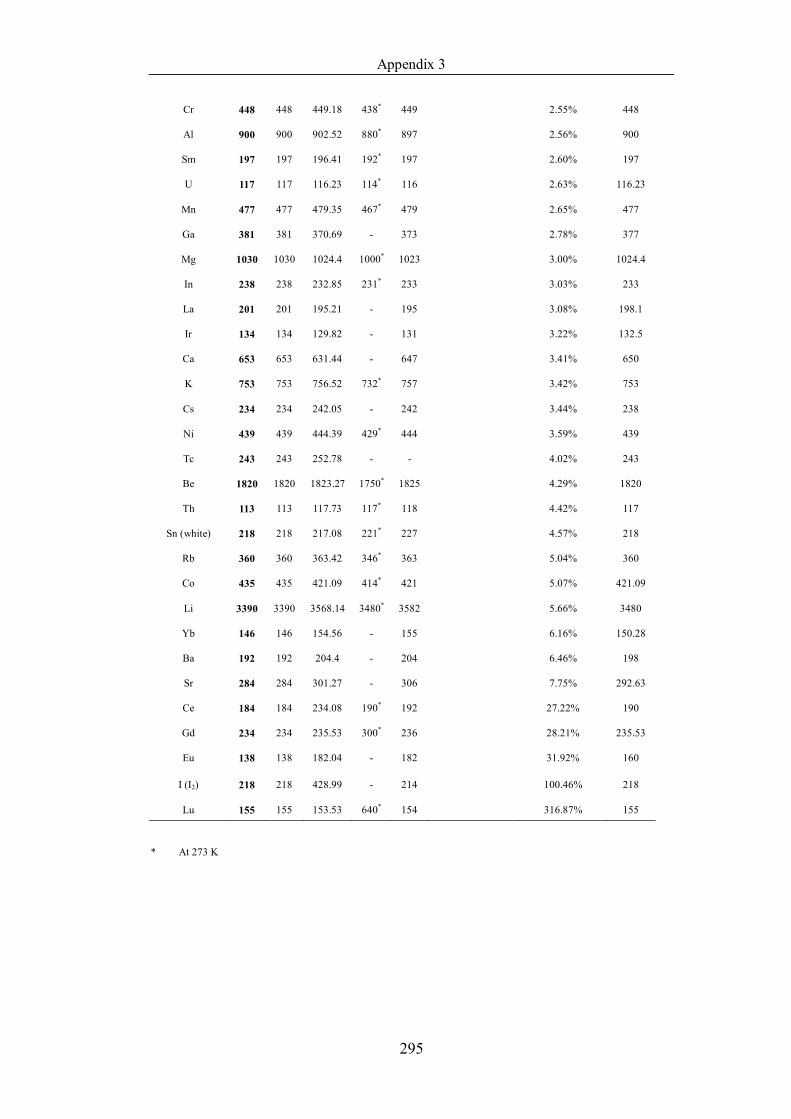
Appendix 3
295
Cr 448 448 449.18 438* 449 2.55% 448
Al 900 900 902.52 880* 897 2.56% 900
Sm 197 197 196.41 192* 197 2.60% 197
U 117 117 116.23 114* 116 2.63% 116.23
Mn 477 477 479.35 467* 479 2.65% 477
Ga 381 381 370.69 - 373 2.78% 377
Mg 1030 1030 1024.4 1000* 1023 3.00% 1024.4
In 238 238 232.85 231* 233 3.03% 233
La 201 201 195.21 - 195 3.08% 198.1
Ir 134 134 129.82 - 131 3.22% 132.5
Ca 653 653 631.44 - 647 3.41% 650
K 753 753 756.52 732* 757 3.42% 753
Cs 234 234 242.05 - 242 3.44% 238
Ni 439 439 444.39 429* 444 3.59% 439
Tc 243 243 252.78 - - 4.02% 243
Be 1820 1820 1823.27 1750* 1825 4.29% 1820
Th 113 113 117.73 117* 118 4.42% 117
Sn (white) 218 218 217.08 221* 227 4.57% 218
Rb 360 360 363.42 346* 363 5.04% 360
Co 435 435 421.09 414* 421 5.07% 421.09
Li 3390 3390 3568.14 3480* 3582 5.66% 3480
Yb 146 146 154.56 - 155 6.16% 150.28
Ba 192 192 204.4 - 204 6.46% 198
Sr 284 284 301.27 - 306 7.75% 292.63
Ce 184 184 234.08 190* 192 27.22% 190
Gd 234 234 235.53 300* 236 28.21% 235.53
Eu 138 138 182.04 - 182 31.92% 160
I (I2) 218 218 428.99 - 214 100.46% 218
Lu 155 155 153.53 640* 154 316.87% 155
* At 273 K
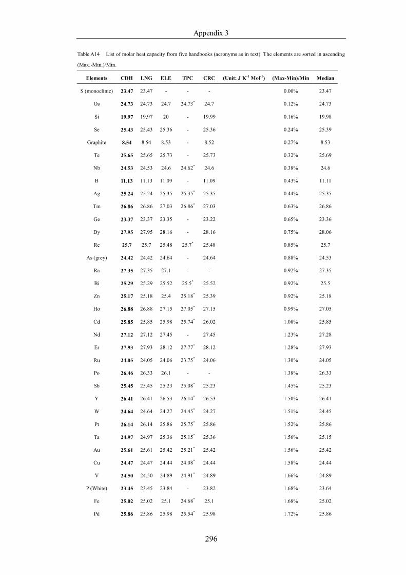
Appendix 3
296
Table A14 List of molar heat capacity from five handbooks (acronyms as in text). The elements are sorted in ascending
(Max.-Min.)/Min.
Elements CDH LNG ELE TPC CRC (Unit: J K-1 Mol-1) (Max-Min)/Min Median
S (monoclinic) 23.47 23.47 - - - 0.00% 23.47
Os 24.73 24.73 24.7 24.73* 24.7 0.12% 24.73
Si 19.97 19.97 20 - 19.99 0.16% 19.98
Se 25.43 25.43 25.36 - 25.36 0.24% 25.39
Graphite 8.54 8.54 8.53 - 8.52 0.27% 8.53
Te 25.65 25.65 25.73 - 25.73 0.32% 25.69
Nb 24.53 24.53 24.6 24.62* 24.6 0.38% 24.6
B 11.13 11.13 11.09 - 11.09 0.43% 11.11
Ag 25.24 25.24 25.35 25.35* 25.35 0.44% 25.35
Tm 26.86 26.86 27.03 26.86* 27.03 0.63% 26.86
Ge 23.37 23.37 23.35 - 23.22 0.65% 23.36
Dy 27.95 27.95 28.16 - 28.16 0.75% 28.06
Re 25.7 25.7 25.48 25.7* 25.48 0.85% 25.7
As (grey) 24.42 24.42 24.64 - 24.64 0.88% 24.53
Ra 27.35 27.35 27.1 - - 0.92% 27.35
Bi 25.29 25.29 25.52 25.5* 25.52 0.92% 25.5
Zn 25.17 25.18 25.4 25.18* 25.39 0.92% 25.18
Ho 26.88 26.88 27.15 27.05* 27.15 0.99% 27.05
Cd 25.85 25.85 25.98 25.74* 26.02 1.08% 25.85
Nd 27.12 27.12 27.45 - 27.45 1.23% 27.28
Er 27.93 27.93 28.12 27.77* 28.12 1.28% 27.93
Ru 24.05 24.05 24.06 23.75* 24.06 1.30% 24.05
Po 26.46 26.33 26.1 - - 1.38% 26.33
Sb 25.45 25.45 25.23 25.08* 25.23 1.45% 25.23
Y 26.41 26.41 26.53 26.14* 26.53 1.50% 26.41
W 24.64 24.64 24.27 24.45* 24.27 1.51% 24.45
Pt 26.14 26.14 25.86 25.75* 25.86 1.52% 25.86
Ta 24.97 24.97 25.36 25.15* 25.36 1.56% 25.15
Au 25.61 25.61 25.42 25.21* 25.42 1.56% 25.42
Cu 24.47 24.47 24.44 24.08* 24.44 1.58% 24.44
V 24.50 24.50 24.89 24.91* 24.89 1.66% 24.89
P (White) 23.45 23.45 23.84 - 23.82 1.68% 23.64
Fe 25.02 25.02 25.1 24.68* 25.1 1.68% 25.02
Pd 25.86 25.86 25.98 25.54* 25.98 1.72% 25.86
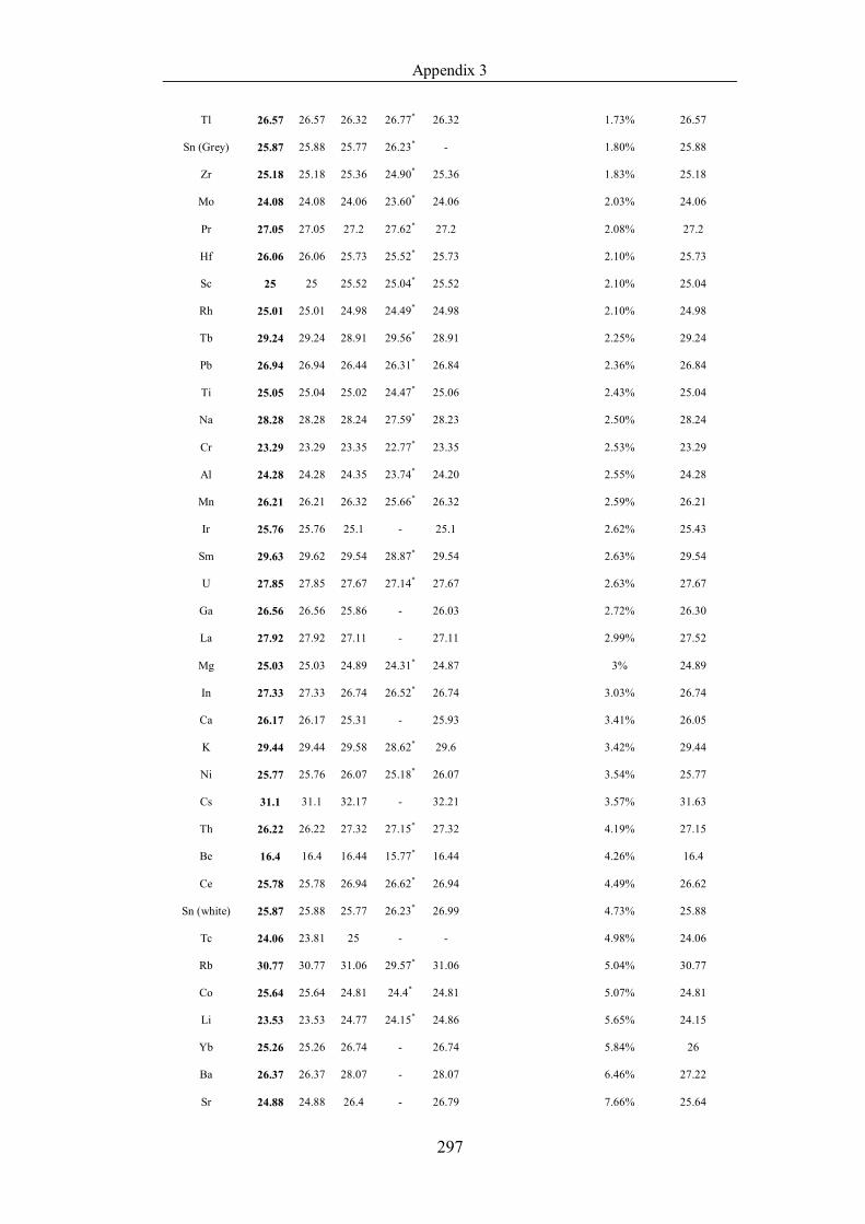
Appendix 3
297
Tl 26.57 26.57 26.32 26.77* 26.32 1.73% 26.57
Sn (Grey) 25.87 25.88 25.77 26.23* - 1.80% 25.88
Zr 25.18 25.18 25.36 24.90* 25.36 1.83% 25.18
Mo 24.08 24.08 24.06 23.60* 24.06 2.03% 24.06
Pr 27.05 27.05 27.2 27.62* 27.2 2.08% 27.2
Hf 26.06 26.06 25.73 25.52* 25.73 2.10% 25.73
Sc 25 25 25.52 25.04* 25.52 2.10% 25.04
Rh 25.01 25.01 24.98 24.49* 24.98 2.10% 24.98
Tb 29.24 29.24 28.91 29.56* 28.91 2.25% 29.24
Pb 26.94 26.94 26.44 26.31* 26.84 2.36% 26.84
Ti 25.05 25.04 25.02 24.47* 25.06 2.43% 25.04
Na 28.28 28.28 28.24 27.59* 28.23 2.50% 28.24
Cr 23.29 23.29 23.35 22.77* 23.35 2.53% 23.29
Al 24.28 24.28 24.35 23.74* 24.20 2.55% 24.28
Mn 26.21 26.21 26.32 25.66* 26.32 2.59% 26.21
Ir 25.76 25.76 25.1 - 25.1 2.62% 25.43
Sm 29.63 29.62 29.54 28.87* 29.54 2.63% 29.54
U 27.85 27.85 27.67 27.14* 27.67 2.63% 27.67
Ga 26.56 26.56 25.86 - 26.03 2.72% 26.30
La 27.92 27.92 27.11 - 27.11 2.99% 27.52
Mg 25.03 25.03 24.89 24.31* 24.87 3% 24.89
In 27.33 27.33 26.74 26.52* 26.74 3.03% 26.74
Ca 26.17 26.17 25.31 - 25.93 3.41% 26.05
K 29.44 29.44 29.58 28.62* 29.6 3.42% 29.44
Ni 25.77 25.76 26.07 25.18* 26.07 3.54% 25.77
Cs 31.1 31.1 32.17 - 32.21 3.57% 31.63
Th 26.22 26.22 27.32 27.15* 27.32 4.19% 27.15
Be 16.4 16.4 16.44 15.77* 16.44 4.26% 16.4
Ce 25.78 25.78 26.94 26.62* 26.94 4.49% 26.62
Sn (white) 25.87 25.88 25.77 26.23* 26.99 4.73% 25.88
Tc 24.06 23.81 25 - - 4.98% 24.06
Rb 30.77 30.77 31.06 29.57* 31.06 5.04% 30.77
Co 25.64 25.64 24.81 24.4* 24.81 5.07% 24.81
Li 23.53 23.53 24.77 24.15* 24.86 5.65% 24.15
Yb 25.26 25.26 26.74 - 26.74 5.84% 26
Ba 26.37 26.37 28.07 - 28.07 6.46% 27.22
Sr 24.88 24.88 26.4 - 26.79 7.66% 25.64
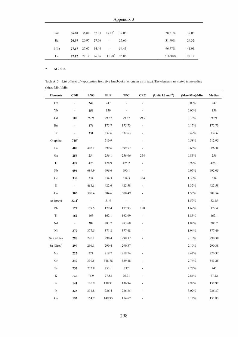
Appendix 3
298
Gd 36.80 36.80 37.03 47.18* 37.03 28.21% 37.03
Eu 20.97 20.97 27.66 - 27.66 31.90% 24.32
I (I2) 27.67 27.67 54.44 - 54.43 96.77% 41.05
Lu 27.12 27.12 26.86 111.98* 26.86 316.90% 27.12
* At 273 K
Table A15 List of heat of vaporization from five handbooks (acronyms as in text). The elements are sorted in ascending
(Max.-Min.)/Min.
Elements CDH LNG ELE TPC CRC (Unit: kJ mol-1) (Max-Min)/Min Median
Tm - 247 247 - - 0.00% 247
Yb - 159 159 - - 0.00% 159
Cd 100 99.9 99.87 99.87 99.9 0.13% 99.9
Eu - 176 175.7 175.73 - 0.17% 175.73
Pr - 331 332.6 332.63 - 0.49% 332.6
Graphite 715* - 710.9 - - 0.58% 712.95
La 400 402.1 399.6 399.57 - 0.63% 399.8
Ga 256 254 256.1 256.06 254 0.83% 256
Ti 427 425 428.9 425.2 - 0.92% 426.1
Nb 694 689.9 696.6 690.1 - 0.97% 692.05
Ge 330 334 334.3 334.3 334 1.30% 334
U - 417.1 422.6 422.58 - 1.32% 422.58
Cu 305 300.4 304.6 300.49 - 1.53% 302.54
As (grey) 32.4* - 31.9 - - 1.57% 32.15
Pb 177 179.5 179.4 177.93 180 1.69% 179.4
Tl 162 165 162.1 162.09 - 1.85% 162.1
Nd - 289 283.7 283.68 - 1.87% 283.7
Ni 379 377.5 371.8 377.48 - 1.94% 377.49
Sn (white) 290 296.1 290.4 290.37 - 2.10% 290.38
Sn (Grey) 290 296.1 290.4 290.37 - 2.10% 290.38
Mn 225 221 219.7 219.74 - 2.41% 220.37
Cr 347 339.5 348.78 339.48 - 2.74% 343.25
Ta 753 732.8 753.1 737 - 2.77% 745
K 79.1 76.9 77.53 76.91 - 2.86% 77.22
Sr 141 136.9 138.91 136.94 - 2.99% 137.92
In 225 231.8 226.4 226.35 - 3.02% 226.37
Ca 153 154.7 149.95 154.67 - 3.17% 153.83
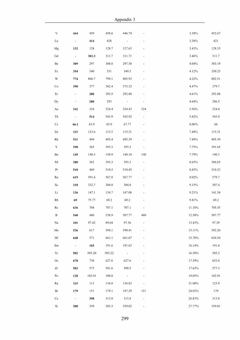
Appendix 3
299
V 444 459 458.6 446.74 - 3.38% 452.67
Lu - 414 428 - - 3.38% 421
Mg 132 128 128.7 127.63 - 3.43% 128.35
Gd - 301.3 311.7 311.71 - 3.46% 311.7
Be 309 297 308.8 297.58 - 4.04% 303.19
Fe 354 340 351 349.5 - 4.12% 350.25
W 774 806.7 799.1 805.93 - 4.22% 802.51
Co 390 377 382.4 373.32 - 4.47% 379.7
Er - 280 292.9 292.88 - 4.61% 292.88
Dy - 280 293 - - 4.64% 286.5
Au 342 324 324.4 324.43 324 5.56% 324.4
Th - 514 543.9 543.92 - 5.82% 543.9
Cs 66.1 63.9 65.9 67.77 - 6.06% 66
Zn 115 123.6 115.3 115.31 - 7.48% 115.31
Rh 531 494 495.4 495.39 - 7.49% 495.39
Y 390 365 393.3 393.3 - 7.75% 391.65
Ba 149 140.3 150.9 140.18 140 7.79% 140.3
Pd 380 362 393.3 393.3 - 8.65% 386.65
Pt 510 469 510.5 510.45 - 8.85% 510.23
Ru 619 591.6 567.8 567.77 - 9.02% 579.7
Sc 310 332.7 304.8 304.8 - 9.15% 307.4
Li 136 147.1 134.7 147.08 - 9.21% 141.54
Rb 69 75.77 69.2 69.2 - 9.81% 69.2
Re 636 704 707.1 707.1 - 11.18% 705.55
B 540 480 538.9 507.77 480 12.50% 507.77
Na 101 97.42 89.04 97.36 - 13.43% 97.39
Mo 536 617 594.1 590.41 - 15.11% 592.26
Hf 648 571 661.1 661.07 - 15.78% 654.54
Sm - 165 191.6 191.63 - 16.14% 191.6
Tc 502 585.20 585.22 - - 16.58% 585.2
Os 678 738 627.6 627.6 - 17.59% 652.8
Zr 502 573 581.6 590.5 - 17.63% 577.3
Po 120 102.91 100.8 - - 19.05% 102.91
Ra 115 113 136.8 136.82 - 21.08% 125.9
Bi 179 151 179.1 187.29 151 24.03% 179
Ce - 398 313.8 313.8 - 26.83% 313.8
Si 300 359 383.3 359.02 - 27.77% 359.01
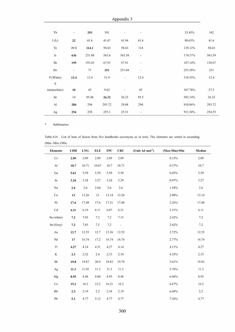
Appendix 3
300
Tb - 293 391 - - 33.45% 342
I (I2) 22 41.6 41.67 41.94 41.6 90.63% 41.6
Te 49.8 114.1 50.63 50.63 114 129.12% 50.63
Ir 636 231.80 563.6 563.58 - 174.37% 563.59
Sb 195 193.43 67.91 67.91 - 187.14% 130.67
Ho - 71 251 251.04 - 253.58% 251
P (White) 12.4 12.4 51.9 - 12.4 318.55% 12.4
S
(monoclinic) 10 45 9.62 - 45 367.78% 27.5
Se 14 95.48 26.32 26.32 95.5 582.14% 26.32
Al 284 294 293.72 29.08 294 910.86% 293.72
Ag 254 258 255.1 25.51 - 911.54% 254.55
* Sublimation
Table A16 List of heat of fusion from five handbooks (acronyms as in text). The elements are sorted in ascending
(Max.-Min.)/Min.
Elements CDH LNG ELE TPC CRC (Unit: kJ mol-1) (Max-Min)/Min Median
Cs 2.09 2.09 2.09 2.09 2.09 0.15% 2.09
Al 10.7 10.71 10.67 10.7 10.71 0.37% 10.7
Ga 5.61 5.59 5.59 5.59 5.59 0.45% 5.59
In 3.26 3.28 3.27 3.26 3.29 0.97% 3.27
Na 2.6 2.6 2.64 2.6 2.6 1.54% 2.6
Cu 13 13.26 13 13.14 13.26 2.00% 13.14
Ni 17.6 17.48 17.6 17.21 17.48 2.26% 17.48
Cd 6.11 6.19 6.11 6.07 6.21 2.31% 6.11
Sn (white) 7.2 7.03 7.2 7.2 7.15 2.42% 7.2
Sn (Grey) 7.2 7.03 7.2 7.2 - 2.42% 7.2
Au 12.7 12.55 12.7 12.36 12.55 2.72% 12.55
Pd 17 16.74 17.2 16.74 16.74 2.77% 16.74
Tl 4.27 4.14 4.31 4.27 4.14 4.11% 4.27
K 2.3 2.32 2.4 2.33 2.34 4.35% 2.33
Sb 19.8 19.87 20.9 19.83 19.79 5.61% 19.83
Ag 11.3 11.95 11.3 11.3 11.3 5.76% 11.3
Mg 8.95 8.48 9.04 8.95 8.48 6.60% 8.95
Co 15.2 16.2 15.2 16.21 16.2 6.67% 16.2
Rb 2.3 2.19 2.2 2.34 2.19 6.68% 2.2
Pb 5.1 4.77 5.12 4.77 4.77 7.36% 4.77
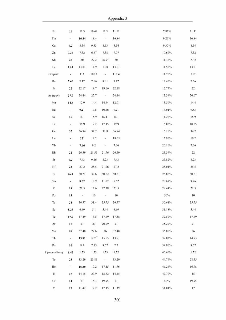
Appendix 3
301
Bi 11 11.3 10.48 11.3 11.11 7.82% 11.11
Tm - 16.84 18.4 - 16.84 9.26% 16.84
Ca 9.2 8.54 9.33 8.53 8.54 9.37% 8.54
Zn 7.36 7.32 6.67 7.38 7.07 10.69% 7.32
Nb 27 30 27.2 26.94 30 11.36% 27.2
Fe 15.4 13.81 14.9 13.8 13.81 11.58% 13.81
Graphite - 117 105.1 - 117.4 11.70% 117
Ba 7.66 7.12 7.66 8.01 7.12 12.46% 7.66
Pt 22 22.17 19.7 19.66 22.18 12.77% 22
As (grey) 27.7 24.44 27.7 - 24.44 13.34% 26.07
Mn 14.6 12.9 14.4 14.64 12.91 13.50% 14.4
Eu - 9.21 10.5 10.46 9.21 14.01% 9.83
Sc 16 14.1 15.9 16.11 14.1 14.28% 15.9
Er - 19.9 17.2 17.15 19.9 16.02% 18.55
Ge 32 36.94 34.7 31.8 36.94 16.15% 34.7
Lu - 22* 19.2 - 18.65 17.96% 19.2
Yb - 7.66 9.2 - 7.66 20.10% 7.66
Rh 22 26.59 21.55 21.76 26.59 23.39% 22
Sr 9.2 7.43 9.16 8.23 7.43 23.82% 8.23
Hf 22 27.2 25.5 21.76 27.2 25.01% 25.5
Si 46.4 50.21 39.6 50.22 50.21 26.82% 50.21
Sm - 8.62 10.9 11.09 8.62 28.67% 9.76
V 18 21.5 17.6 22.78 21.5 29.44% 21.5
Po 13 - 10 - 10 30% 10
Ta 28 36.57 31.4 35.75 36.57 30.61% 35.75
Se 5.23 6.69 5.1 5.44 6.69 31.18% 5.44
Te 17.9 17.49 13.5 17.49 17.38 32.59% 17.49
Zr 17 21 23 20.79 21 35.29% 21
Mo 28 37.48 27.6 36 37.48 35.80% 36
Th - 13.81 19.2** 15.65 13.81 39.03% 14.73
Ra 10 8.5 7.15 8.37 7.7 39.86% 8.37
S (monoclinic) 1.42 1.73 1.23 1.73 1.72 40.60% 1.72
Tc 23 33.29 23.81 - 33.29 44.74% 28.55
Ho - 16.80 17.2 17.15 11.76 46.26% 16.98
Ti 15 14.15 20.9 18.62 14.15 47.70% 15
Cr 14 21 15.3 19.95 21 50% 19.95
Y 17 11.42 17.2 17.15 11.39 51.01% 17
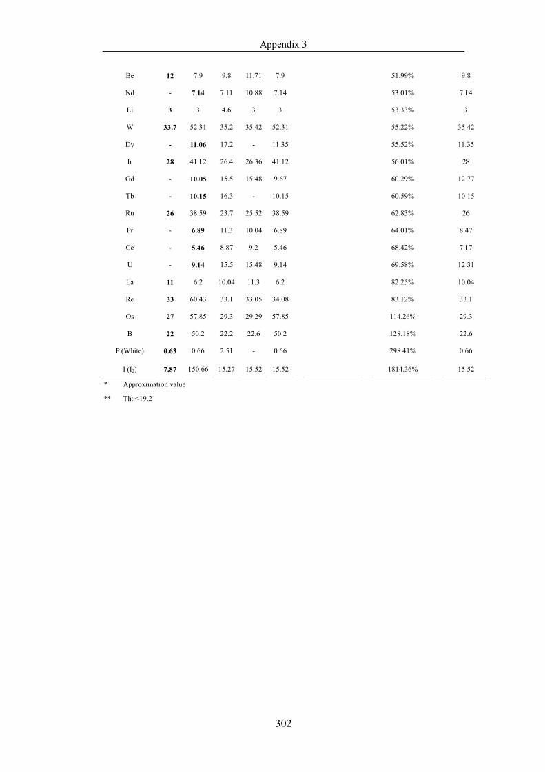
Appendix 3
302
Be 12 7.9 9.8 11.71 7.9 51.99% 9.8
Nd - 7.14 7.11 10.88 7.14 53.01% 7.14
Li 3 3 4.6 3 3 53.33% 3
W 33.7 52.31 35.2 35.42 52.31 55.22% 35.42
Dy - 11.06 17.2 - 11.35 55.52% 11.35
Ir 28 41.12 26.4 26.36 41.12 56.01% 28
Gd - 10.05 15.5 15.48 9.67 60.29% 12.77
Tb - 10.15 16.3 - 10.15 60.59% 10.15
Ru 26 38.59 23.7 25.52 38.59 62.83% 26
Pr - 6.89 11.3 10.04 6.89 64.01% 8.47
Ce - 5.46 8.87 9.2 5.46 68.42% 7.17
U - 9.14 15.5 15.48 9.14 69.58% 12.31
La 11 6.2 10.04 11.3 6.2 82.25% 10.04
Re 33 60.43 33.1 33.05 34.08 83.12% 33.1
Os 27 57.85 29.3 29.29 57.85 114.26% 29.3
B 22 50.2 22.2 22.6 50.2 128.18% 22.6
P (White) 0.63 0.66 2.51 - 0.66 298.41% 0.66
I (I2) 7.87 150.66 15.27 15.52 15.52 1814.36% 15.52
* Approximation value
** Th: <19.2
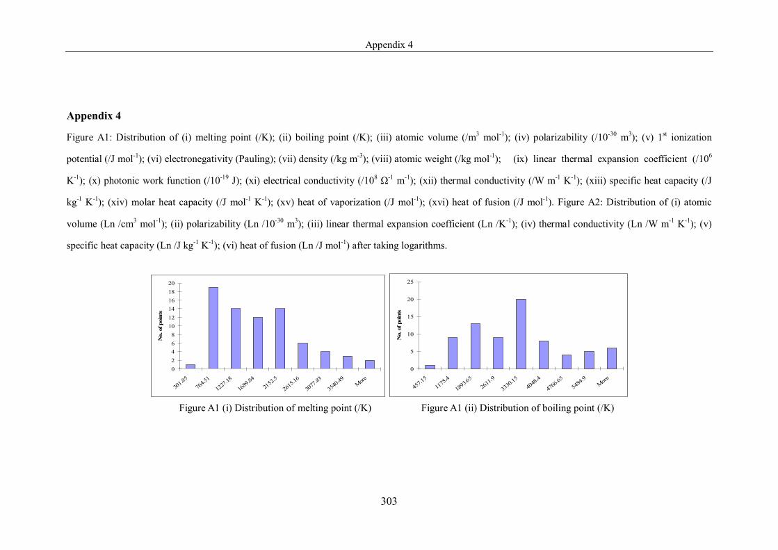
Appendix 4
303
Appendix 4
Figure A1: Distribution of (i) melting point (/K); (ii) boiling point (/K); (iii) atomic volume (/m3 mol-1); (iv) polarizability (/10-30 m3); (v) 1st ionization
potential (/J mol-1); (vi) electronegativity (Pauling); (vii) density (/kg m-3); (viii) atomic weight (/kg mol-1); (ix) linear thermal expansion coefficient (/106
K-1); (x) photonic work function (/10-19 J); (xi) electrical conductivity (/108 Ω-1 m-1); (xii) thermal conductivity (/W m-1 K-1); (xiii) specific heat capacity (/J
kg-1 K-1); (xiv) molar heat capacity (/J mol-1 K-1); (xv) heat of vaporization (/J mol-1); (xvi) heat of fusion (/J mol-1). Figure A2: Distribution of (i) atomic
volume (Ln /cm3 mol-1); (ii) polarizability (Ln /10-30 m3); (iii) linear thermal expansion coefficient (Ln /K-1); (iv) thermal conductivity (Ln /W m-1 K-1); (v)
specific heat capacity (Ln /J kg-1 K-1); (vi) heat of fusion (Ln /J mol-1) after taking logarithms.
02468
101214161820
301.8
576
4.51
1227
.18
1689
.8421
52.5
2615
.16
3077
.83
3540
.49 More
No.
of p
oint
s
0
5
10
15
20
25
457.1
511
75.4
1893
.6526
11.9
3330
.1540
48.4
4766
.6554
84.9
More
No.
of p
oint
s
Figure A1 (i) Distribution of melting point (/K) Figure A1 (ii) Distribution of boiling point (/K)
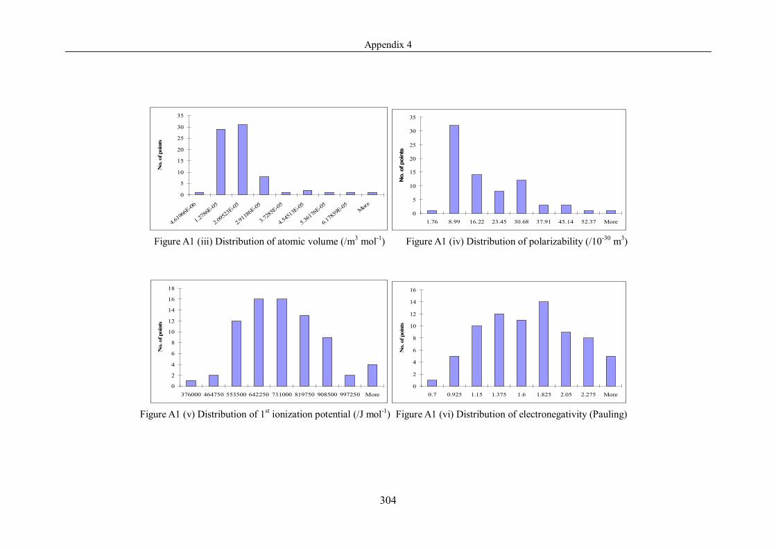
Appendix 4
304
0
5
10
15
20
25
30
35
4.619
66E-06
1.278
6E-05
2.095
23E-05
2.911
86E-05
3.728
5E-05
4.545
13E-05
5.361
76E-05
6.178
39E-05 More
No.
of p
oint
s
0
5
10
15
20
25
30
35
1.76 8.99 16.22 23.45 30.68 37.91 45.14 52.37 More
No.
of p
oint
s
Figure A1 (iii) Distribution of atomic volume (/m3 mol-1) Figure A1 (iv) Distribution of polarizability (/10-30 m3)
0
2
4
6
8
10
12
14
16
18
376000 464750 553500 642250 731000 819750 908500 997250 More
No.
of p
oint
s
0
2
4
6
8
10
12
14
16
0.7 0.925 1.15 1.375 1.6 1.825 2.05 2.275 MoreN
o. o
f poi
nts
Figure A1 (v) Distribution of 1st ionization potential (/J mol-1) Figure A1 (vi) Distribution of electronegativity (Pauling)
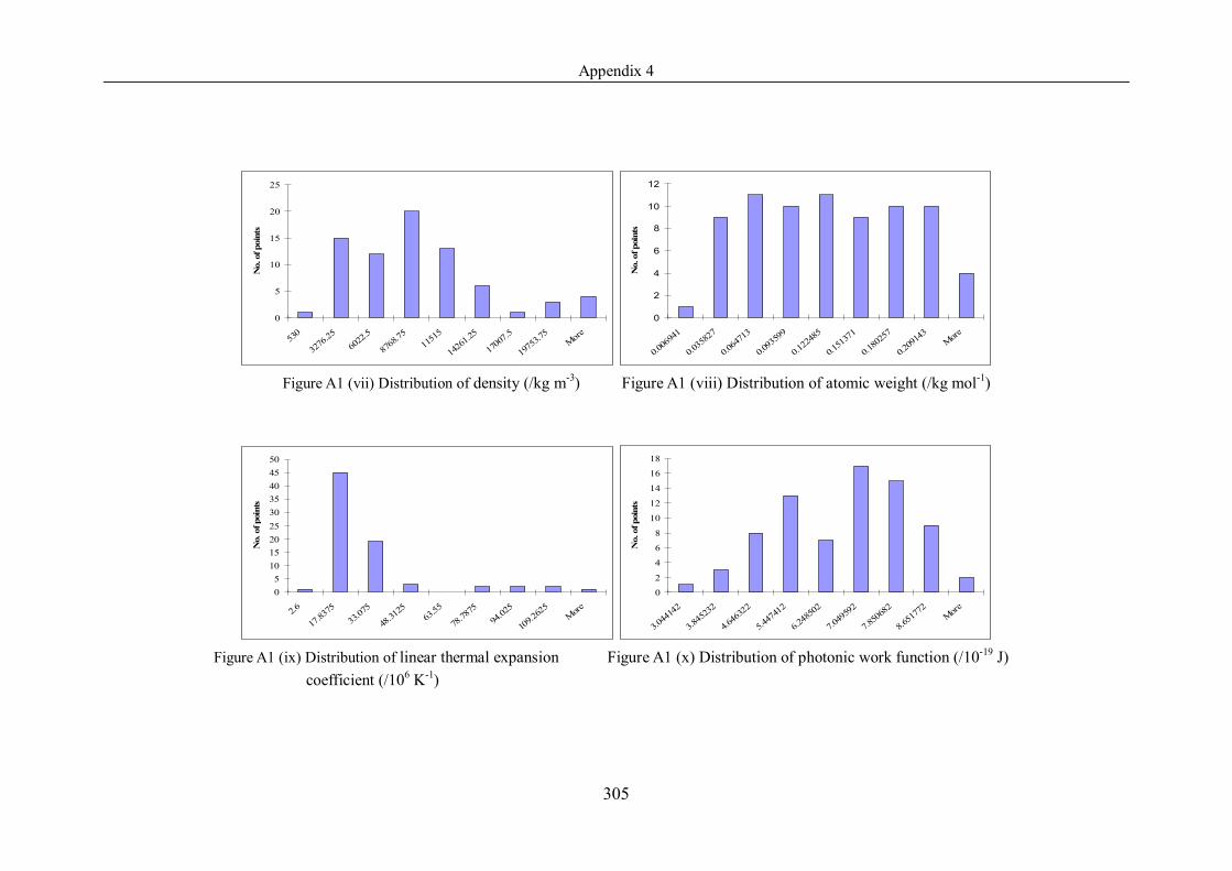
Appendix 4
305
0
5
10
15
20
25
530
3276
.2560
22.5
8768
.7511
515
1426
1.25
1700
7.5
1975
3.75
More
No.
of p
oint
s
0
2
4
6
8
10
12
0.006
941
0.035
827
0.064
713
0.093
599
0.122
485
0.151
371
0.180
257
0.209
143
More
No.
of p
oint
s
Figure A1 (vii) Distribution of density (/kg m-3) Figure A1 (viii) Distribution of atomic weight (/kg mol-1)
05
101520253035404550
2.6
17.83
7533
.075
48.31
2563
.55
78.78
7594
.025
109.2
625
More
No.
of p
oint
s
0
2
4
6
8
10
12
14
16
18
3.044
142
3.845
232
4.646
322
5.447
412
6.248
502
7.049
592
7.850
682
8.651
772
More
No.
of p
oint
s
Figure A1 (ix) Distribution of linear thermal expansion Figure A1 (x) Distribution of photonic work function (/10-19 J) coefficient (/106 K-1)
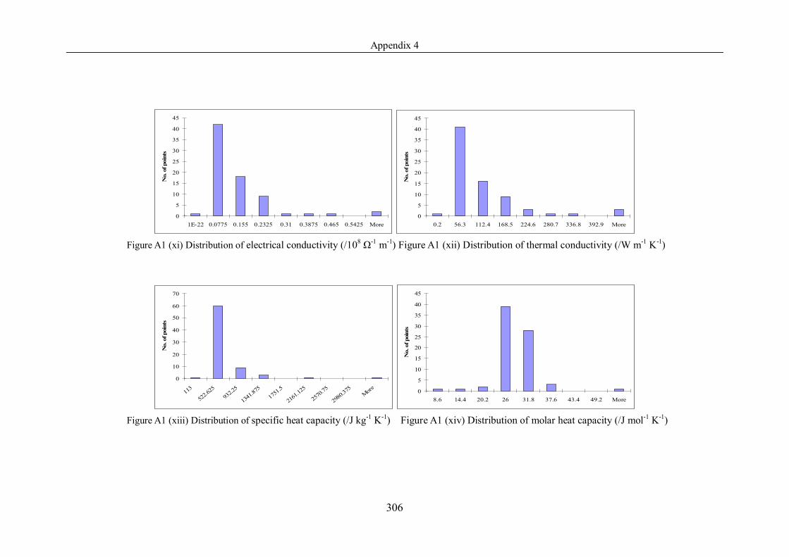
Appendix 4
306
0
5
10
15
20
25
30
35
40
45
1E-22 0.0775 0.155 0.2325 0.31 0.3875 0.465 0.5425 More
No.
of p
oint
s
0
5
10
15
20
25
30
35
40
45
0.2 56.3 112.4 168.5 224.6 280.7 336.8 392.9 More
No.
of p
oint
s
Figure A1 (xi) Distribution of electrical conductivity (/108 Ω-1 m-1) Figure A1 (xii) Distribution of thermal conductivity (/W m-1 K-1)
0
10
20
30
40
50
60
70
113
522.6
2593
2.25
1341
.875
1751
.5
2161
.125
2570
.75
2980
.375
More
No.
of p
oint
s
0
5
10
15
20
25
30
35
40
45
8.6 14.4 20.2 26 31.8 37.6 43.4 49.2 MoreN
o. o
f poi
nts
Figure A1 (xiii) Distribution of specific heat capacity (/J kg-1 K-1) Figure A1 (xiv) Distribution of molar heat capacity (/J mol-1 K-1)
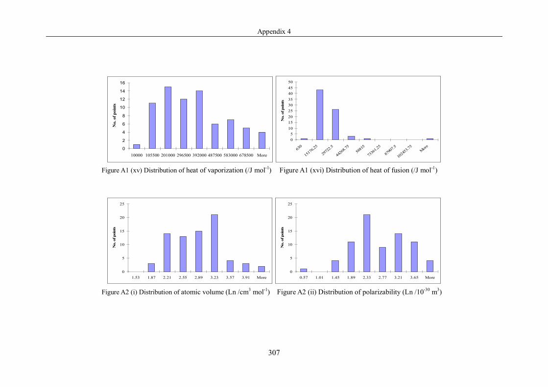
Appendix 4
307
0
2
4
6
8
10
12
14
16
10000 105500 201000 296500 392000 487500 583000 678500 More
No.
of p
oint
s
05
101520253035404550
630
1517
6.25
2972
2.5
4426
8.75
5881
5
7336
1.25
8790
7.5
1024
53.75 More
No.
of p
oint
s
Figure A1 (xv) Distribution of heat of vaporization (/J mol-1) Figure A1 (xvi) Distribution of heat of fusion (/J mol-1)
0
5
10
15
20
25
1.53 1.87 2.21 2.55 2.89 3.23 3.57 3.91 More
No.
of p
oint
s
0
5
10
15
20
25
0.57 1.01 1.45 1.89 2.33 2.77 3.21 3.65 MoreN
o. o
f poi
nts
Figure A2 (i) Distribution of atomic volume (Ln /cm3 mol-1) Figure A2 (ii) Distribution of polarizability (Ln /10-30 m3)
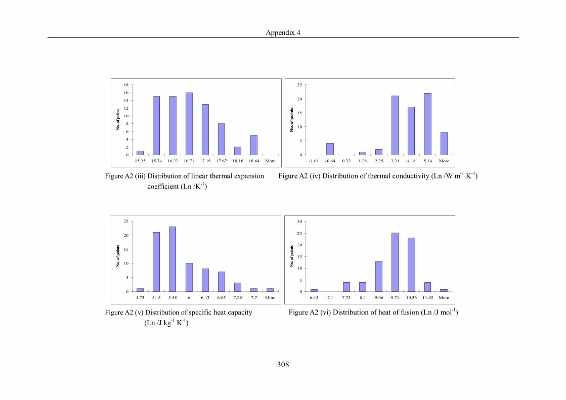
Appendix 4
308
0
2
4
6
8
10
12
14
16
18
15.25 15.74 16.22 16.71 17.19 17.67 18.16 18.64 More
No.
of p
oint
s
0
5
10
15
20
25
-1.61 -0.64 0.32 1.28 2.25 3.21 4.18 5.14 More
No.
of p
oint
s
Figure A2 (iii) Distribution of linear thermal expansion Figure A2 (iv) Distribution of thermal conductivity (Ln /W m-1 K-1) coefficient (Ln /K-1)
0
5
10
15
20
25
4.73 5.15 5.58 6 6.43 6.85 7.28 7.7 More
No.
of p
oint
s
0
5
10
15
20
25
30
6.45 7.1 7.75 8.4 9.06 9.71 10.36 11.02 MoreN
o. o
f poi
nts
Figure A2 (v) Distribution of specific heat capacity Figure A2 (vi) Distribution of heat of fusion (Ln /J mol-1) (Ln /J kg-1 K-1)
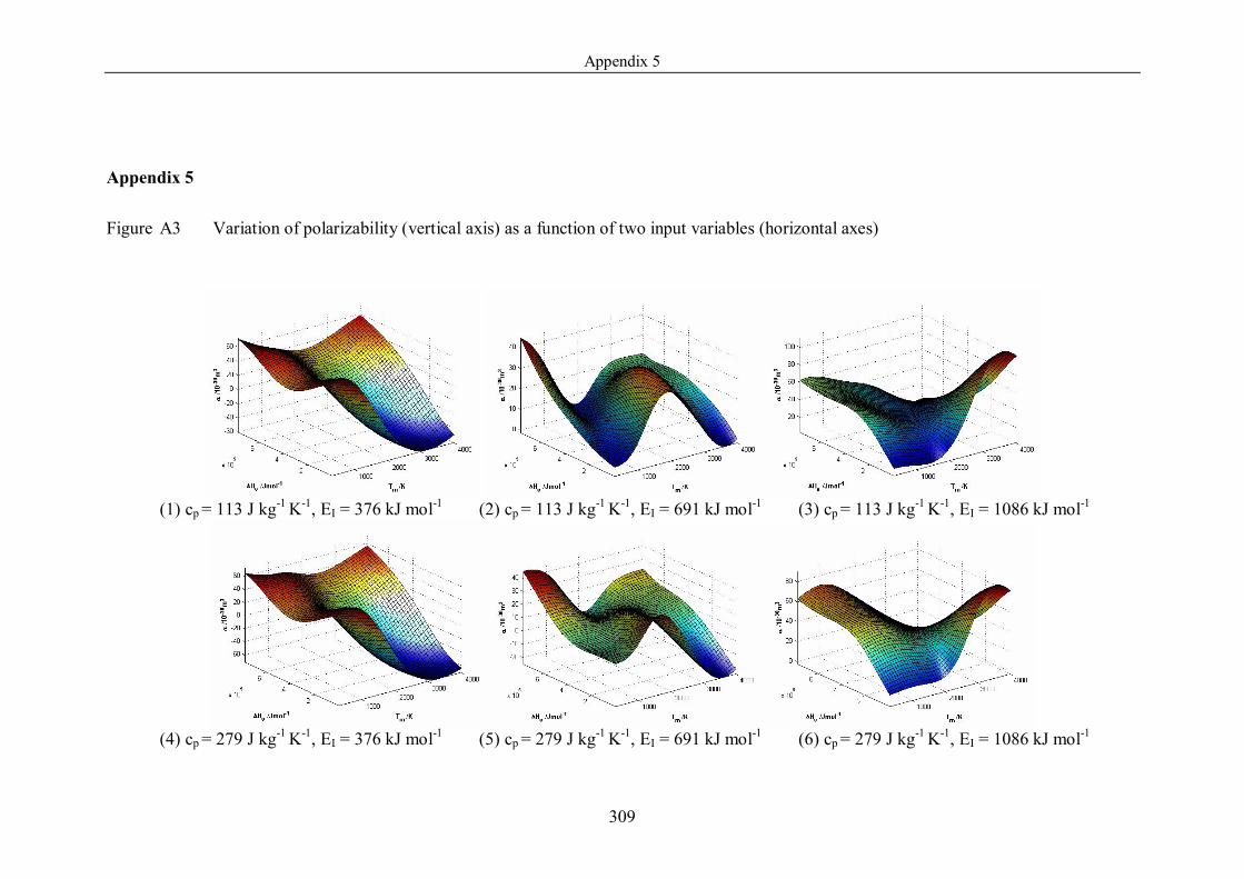
Appendix 5
309
Appendix 5
Figure A3 Variation of polarizability (vertical axis) as a function of two input variables (horizontal axes)
(1) cp = 113 J kg-1 K-1, EI = 376 kJ mol-1 (2) cp = 113 J kg-1 K-1, EI = 691 kJ mol-1 (3) cp = 113 J kg-1 K-1, EI = 1086 kJ mol-1
(4) cp = 279 J kg-1 K-1, EI = 376 kJ mol-1 (5) cp = 279 J kg-1 K-1, EI = 691 kJ mol-1 (6) cp = 279 J kg-1 K-1, EI = 1086 kJ mol-1
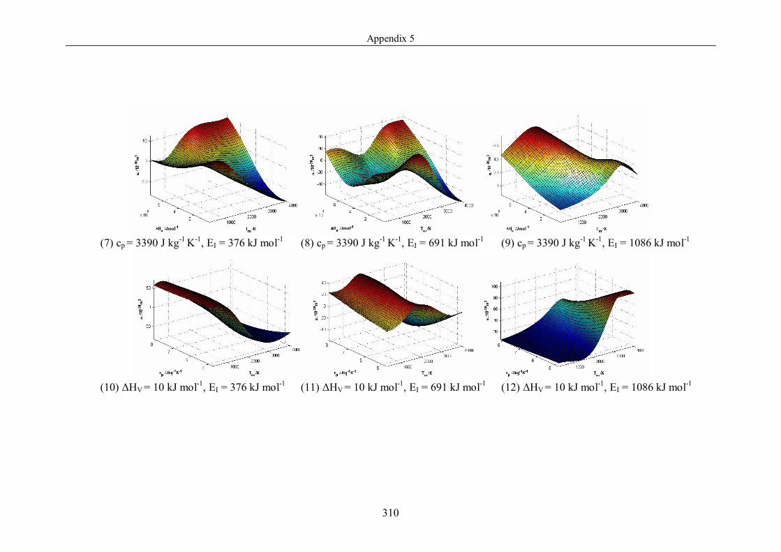
Appendix 5
310
(7) cp = 3390 J kg-1 K-1, EI = 376 kJ mol-1 (8) cp = 3390 J kg-1 K-1, EI = 691 kJ mol-1 (9) cp = 3390 J kg-1 K-1, EI = 1086 kJ mol-1
(10) ΔHV = 10 kJ mol-1, EI = 376 kJ mol-1 (11) ΔHV = 10 kJ mol-1, EI = 691 kJ mol-1 (12) ΔHV = 10 kJ mol-1, EI = 1086 kJ mol-1
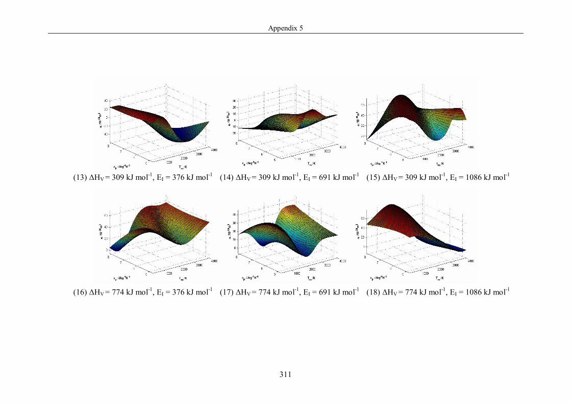
Appendix 5
311
(13) ΔHV = 309 kJ mol-1, EI = 376 kJ mol-1 (14) ΔHV = 309 kJ mol-1, EI = 691 kJ mol-1 (15) ΔHV = 309 kJ mol-1, EI = 1086 kJ mol-1
(16) ΔHV = 774 kJ mol-1, EI = 376 kJ mol-1 (17) ΔHV = 774 kJ mol-1, EI = 691 kJ mol-1 (18) ΔHV = 774 kJ mol-1, EI = 1086 kJ mol-1
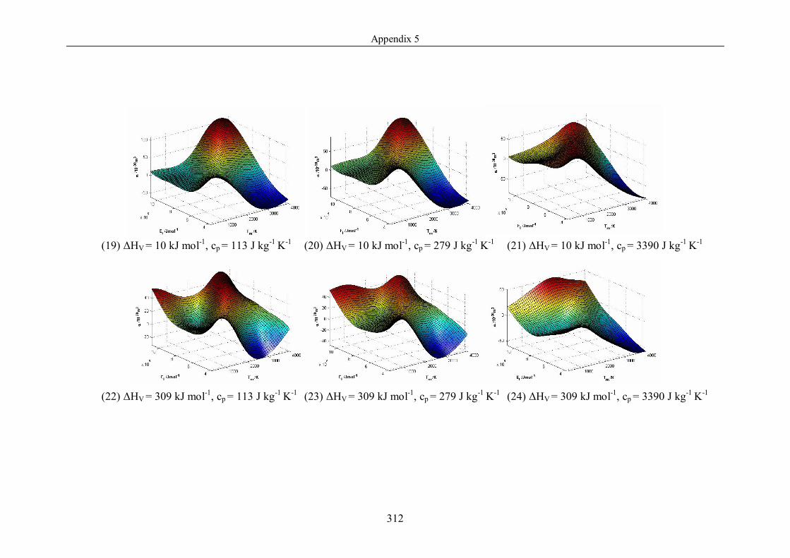
Appendix 5
312
(19) ΔHV = 10 kJ mol-1, cp = 113 J kg-1 K-1 (20) ΔHV = 10 kJ mol-1, cp = 279 J kg-1 K-1 (21) ΔHV = 10 kJ mol-1, cp = 3390 J kg-1 K-1
(22) ΔHV = 309 kJ mol-1, cp = 113 J kg-1 K-1 (23) ΔHV = 309 kJ mol-1, cp = 279 J kg-1 K-1 (24) ΔHV = 309 kJ mol-1, cp = 3390 J kg-1 K-1
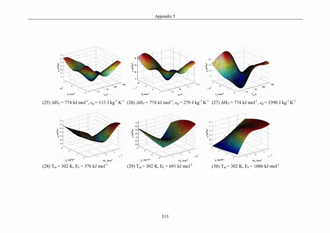
Appendix 5
313
(25) ΔHV = 774 kJ mol-1, cp = 113 J kg-1 K-1 (26) ΔHV = 774 kJ mol-1, cp = 279 J kg-1 K-1 (27) ΔHV = 774 kJ mol-1, cp = 3390 J kg-1 K-1
(28) Tm = 302 K, EI = 376 kJ mol-1 (29) Tm = 302 K, EI = 691 kJ mol-1 (30) Tm = 302 K, EI = 1086 kJ mol-1
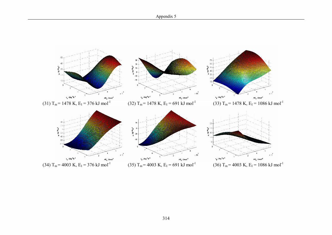
Appendix 5
314
(31) Tm = 1478 K, EI = 376 kJ mol-1 (32) Tm = 1478 K, EI = 691 kJ mol-1 (33) Tm = 1478 K, EI = 1086 kJ mol-1
(34) Tm = 4003 K, EI = 376 kJ mol-1 (35) Tm = 4003 K, EI = 691 kJ mol-1 (36) Tm = 4003 K, EI = 1086 kJ mol-1
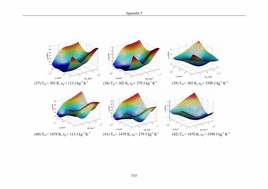
Appendix 5
315
(37) Tm = 302 K, cp = 113 J kg-1 K-1 (38) Tm = 302 K, cp = 279 J kg-1 K-1 (39) Tm = 302 K, cp = 3390 J kg-1 K-1
(40) Tm = 1478 K, cp = 113 J kg-1 K-1 (41) Tm = 1478 K, cp = 279 J kg-1 K-1 (42) Tm = 1478 K, cp = 3390 J kg-1 K-1
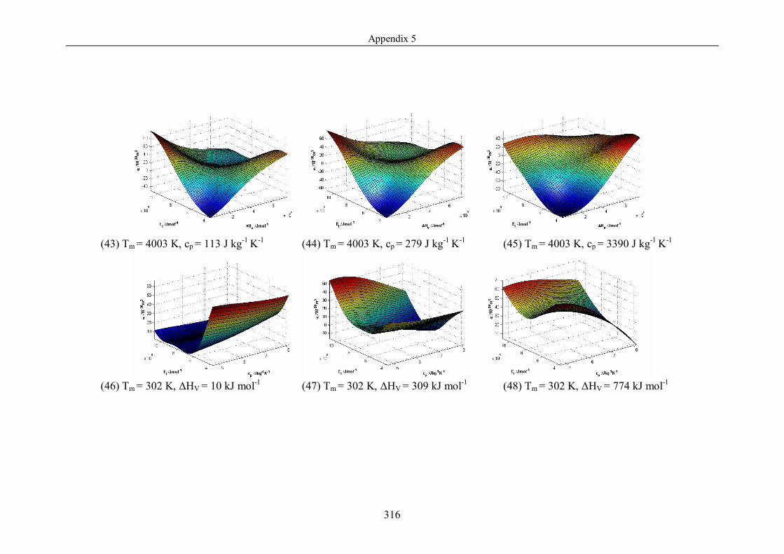
Appendix 5
316
(43) Tm = 4003 K, cp = 113 J kg-1 K-1 (44) Tm = 4003 K, cp = 279 J kg-1 K-1 (45) Tm = 4003 K, cp = 3390 J kg-1 K-1
(46) Tm = 302 K, ΔHV = 10 kJ mol-1 (47) Tm = 302 K, ΔHV = 309 kJ mol-1 (48) Tm = 302 K, ΔHV = 774 kJ mol-1
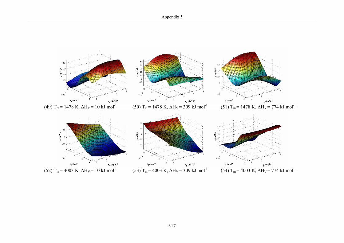
Appendix 5
317
(49) Tm = 1478 K, ΔHV = 10 kJ mol-1 (50) Tm = 1478 K, ΔHV = 309 kJ mol-1 (51) Tm = 1478 K, ΔHV = 774 kJ mol-1
(52) Tm = 4003 K, ΔHV = 10 kJ mol-1 (53) Tm = 4003 K, ΔHV = 309 kJ mol-1 (54) Tm = 4003 K, ΔHV = 774 kJ mol-1


