Embed Size (px)
Citation preview

© 2009
Sock Hwan Lee
All Rights Reserved

Tax Competition among Governments and the Effects on Government
Performance: Empirical Evidence from Local Governments in New Jersey
By Sock Hwan Lee
A dissertation submitted to the Graduate School-Newark
Rutgers, The State University of New Jersey
in partial fulfillment of requirements
for the degree of Doctor of Philosophy
Ph.D. Program in Public Administration
Written under the direction of Dr. Peter D. Loeb
and approved by
Peter D. Loeb Professor, Department of Economics, Rutgers-Newark
Marc Holzer Dean, School of Public Affairs and Administration, Rutgers-Newark
Gerald J. Miller Professor, School of Public Affairs, Arizona State University
Tae-Ho Eom Assistant Professor, Department of Public Administration, Yonsei University
Jeffrey P. Cohen Associate Professor, Department of Economics, Finance, and Insurance, University of Hartford
Newark, New Jersey
May, 2009
ii
Tax Competition among Governments and the Effects on Government
Performance: Empirical Evidence from Local Governments in New Jersey
By Sock Hwan Lee
Thesis director: Dr. Peter D. Loeb
This thesis addresses two fundamental issues highlighted in the literature on
competition among governments: 1) Do local governments engage in tax competition?
and 2) What are the effects of competition on government performance?
In a multi-level government system, we can observe two types of competition:
inter-jurisdictional competition between the same level of governments and intra-
jurisdictional competition between governments sharing the same tax base. To examine
the presence of competition and the effects on government performance, we estimate
several equations using data on New Jersey local governments. New Jersey is an optimal
location to examine both types of competition simultaneously given its diversity in
political institutions, its highly fragmented local governmental structure, and the property
tax base sharing between municipalities, school districts, and counties.
This study contributes to the literature on government competition by examining
the presence of both types of competition within a comprehensive framework and the
effect of competition in terms of government efficiency. To investigate the presence of
both inter- and intra-jurisdictional competition, we estimate property tax rate models
which relate municipal tax rates to those of competing jurisdictions, school districts, and

iii
counties, using spatial econometric techniques. The spatial regression results provide
strong evidence for the existence of both types of competition, showing that
municipalities react negatively to the changes in county tax rates and positively to the
changes in tax rates of school districts and competing municipalities.
We also examine the effects of competition among governments on government
performance. More specifically, we estimate the effect of competition on the combined
tax rates of municipalities and school districts, on property values, and on DEA technical
efficiency scores. We find that inter-jurisdictional competition leads to lower tax rates
and enhances both allocative and technical efficiency. This confirms the beneficial effect
espoused by Tiebout, the Leviathan hypothesis, and yardstick competition, but not the
harmful effect of the tax competition theory. We also find that school district
consolidation reduces tax rates but does not have any significant effect on allocative and
technical efficiency. In addition, we find that school budget referendums lower tax rates
and lead to allocative efficiency.

iv
Acknowledgements
Completing this dissertation would not have been possible without the support of
a number of people. First and foremost, I would like to thank my dissertation adviser, Dr.
Peter D. Loeb for his guidance, support, and commitment throughout this lengthy process.
I would also like to record my sincere thanks and gratitude to the other members of my
dissertation committee: Dr. Marc Holzer, Dr. Gerald J. Miller, Dr. Tae-Ho Eom, and Dr.
Jeffrey P. Cohen.
I benefited from the help of other individuals at the Department of Public
Administration. I would like to thank Gail Daniels, Melissa Rivera, and Madelene Perez.
I would also like to thank the following fellow graduate students who became great
friends in the preceding years: Audrey Redding-Raines, Chulwoo Kim, Dong Chul Shim,
Dong Young Rhee, Jong One Cheong, Weerasak Krueathep, Weiwei Lin, and especially
Jonathan Woolley for his help.
I would like to thank my parents, mother-in-law, brother, sisters, brothers-in-law,
and sisters-in-law for their love, support, and encouragement. Finally, I would like to
thank my wife, Mi-Sun Jeong and my source of joy and hope for the future, my son, Ji-
Woo Lee. I could not have completed this dissertation without my wife’s love, patience,
and understanding. I would like to dedicate this dissertation to my parents and my wife.

v
Table of Contents
Chapter I. Introduction......................................................................................................... 1
Chapter II. Alternative Theories of Fiscal Competition among Governments ............... 6
2-1. Tiebout – The Origin of Inter-jurisdictional Competition Theory .......................................... 8
2-2. Tax Competition.................................................................................................................. 9
2-3. Leviathan Literature .......................................................................................................... 33
2-4. Yardstick Competition ....................................................................................................... 53
2-5. Intra-jurisdictional Competition.......................................................................................... 71
2-6. Conclusion ........................................................................................................................ 89
Chapter III. Structure and Budget Process of Local Governments in New Jersey ..... 99
3-1. Structure of Local Governments ....................................................................................... 99
3-2. Expenditures and Revenues of Local Governments ....................................................... 126
3-3. Property Tax Administration............................................................................................ 137
3-4. Conclusion ...................................................................................................................... 155
Chapter IV. Hypotheses, Research Models, and Data..................................................158
4-1. Hypotheses..................................................................................................................... 159
4-2. Definition of Public Market .............................................................................................. 172
4-3. Research Models ............................................................................................................ 179
4-4. Source of Data and Descriptive Statistics ....................................................................... 219
Chapter V. Empirical Results ..........................................................................................223
5-1. Existence of Tax Competition ......................................................................................... 223
5-2. Effect of Competition on Property Tax Rates .................................................................. 237
5-3. Effect of Competition on Allocative Efficiency ................................................................. 243
5-4. Effect of Competition on Technical Efficiency ................................................................. 248
Chapter VI. Conclusion.................................................................................................... 254
6-1. Summary of Empirical Findings ...................................................................................... 254
6-2. Contribution to the Existing Literature ............................................................................. 257
6-3. Limitations and Recommendations for Future Researches............................................. 258

vi
Appendices .......................................................................................................................260
Appendix A. First-Stage Regression Outputs of Non-Spatial Model ...................................... 260
Appendix B. First-Stage Regression Outputs of Spatial Lag Model by 2SLS......................... 262
Appendix C. SARMA Municipal Tax Rate Model with County Weights by GMM.................... 271
Appendix D. Combined Tax Rate Model by Random-Effects................................................. 272
Appendix E. Property Value Model by GEE ........................................................................... 276
Appendix F. Property Value Model by Random-Effects ......................................................... 280
Bibliography......................................................................................................................284
Curriculum Vitae...............................................................................................................297

vii
List of Tables
Table 2-1. Summary of Empirical Studies on Tax Competition ................................................ 31 Table 2-2. Summary of Empirical Studies on Leviathan Hypothesis ........................................ 51 Table 2-3. Summary of Empirical Studies on Yardstick Competition ....................................... 69 Table 2-4. Summary of Empirical Studies on Intra-jurisdictional Competition .......................... 88 Table 2-5. Summary of Alternative Theories on Inter-jurisdictional Competition ...................... 89 Table 3-1. County Classification Criteria ................................................................................ 104 Table 3-2. Governmental Structure and Classification of the County..................................... 105 Table 3-3. Forms of Municipal Government in 2005 .............................................................. 112 Table 3-4. Forms of Municipal Government by General Pattern of Organization in 2005 ...... 115 Table 3-5. Public Schools and Enrollments (2000-2005) ....................................................... 117 Table 3-6. Number of School Districts (2000-2007) ............................................................... 119 Table 3-7. Characteristics of Type I and II School Districts.................................................... 121 Table 3-8. Number of Special Districts in New Jersey ........................................................... 125 Table 3-9. State and Local Government Expenditure by Functions (2003-04 ~ 2005-06)...... 130 Table 3-10. Local Government Spending by the Type of Local Government (2004-2007)..... 132 Table 3-11. State and Local Government Revenues by Source (2003-04 ~ 2005-06)........... 135 Table 3-12. Revenues by the Type of Local Government (2000-2007).................................. 137 Table 3-13. Property Tax Base (2000-2007) .......................................................................... 149 Table 3-14. Property Tax Rates by the Type of Local Government (2000-2007) ................... 152 Table 3-15. Property Tax Collections by the Type of Local Government (2000-2007)........... 154 Table 4-1. Number of Competitors by Public Market.............................................................. 178 Table 4-2. Descriptive Statistics and Data Source ................................................................. 221 Table 5-1. Spatial Autocorrelation in Residuals of the Non-spatial Municipal Tax Rate Model
............................................................................................................................. 230 Table 5-2. Results of Municipal Tax Rate Models (2004)....................................................... 236 Table 5-3. Results of Combined Municipal-School District Tax Rate Model by GEE (2001-
2004) .................................................................................................................... 242 Table 5-4. Results of Hedonic Property Value Model by OLS (2004) .................................... 247 Table 5-5. Summary Statistics for the DEA Technical Efficiency Score (2001-2004)............. 249 Table 5-6. Results of Technical Efficiency Model by Tobit Random-Effects (2001-2004) ...... 253

viii
List of Figures
Figure 5-1. Property Tax Rates by the Type of Local Government (2004) ............................. 225 Figure 5-2. Moran I Statistics and Moran Scatter Plot for Municipal Property Tax Rates (2004)
............................................................................................................................. 227

1
Chapter I. Introduction
Competition among governments can be defined as “rivalrous behavior in which
each government attempts to win some scarce benefit resources” or “avoid a particular
cost” (ACIR, 1991, p.xv). In a multi-tier government system, two types of competition
can take place: horizontal and vertical competition. The horizontal or inter-jurisdictional
competition entails competition among the same level of governments. On the other hand,
vertical or intra-jurisdictional competition, involves competition between governments
having different powers.
The efficiency implications of inter-jurisdictional competition have been explored
in the public finance literature since Tiebout’s (1956) seminal paper, “A Pure Theory of
Local Expenditures.” According to Tiebout, if local governments compete with each
other and citizens are able to “vote with their feet,” there may be fairly strong pressures
for local governments to respond to the wishes of the resident. Moreover, competition
among local governments would create pressures to increase productivity and reduce
waste in order to avoid becoming uncompetitive relative to other local governments.
While Tiebout’s paper was a purely theoretical piece, it has had wide theoretical and
empirical applications.
Depending on the assumed channel of competition, on the developmental history,
and on the assumption of government behavior, the existing studies on inter-jurisdictional
competition can be further grouped into three broad categories: tax competition,
Leviathan hypothesis, and yardstick competition. The three models have different views
on the mechanisms in which competition arises and the effect of competition on
government performance. The Leviathan hypothesis and tax competition models are

2
based on the mobility of residents, capital, or factors of production, while yardstick
competition arises through the fact that citizen-voters comparatively evaluate the
performance of politicians in an election. In terms of effects of competition, all models
have in common a prediction that competition reduces tax rates and the provision of
public services, but they seem to interpret differently the reduced tax rates and public
services. While the Leviathan hypothesis and yardstick competition view the reduced tax
rates and public services as the elimination of waste, tax competition regards it as the loss
of welfare.
More recently, attention has turned to intra-jurisdictional competition arising from
tax base sharing and overlapping services between different levels of government. The
intra-jurisdictional competition literature analyzes the equilibrium tax levels and the
reaction of the lower level of government to the policy changes of the higher level of
government. Most equilibrium analyses have in common the result that an increase in
taxes by one level of government results in a reduction in revenue to the other level and
this negative externality leads to excessive taxation compared with coordinated or unitary
government policies. The intra-jurisdictional competition literature also theoretically
investigates the reaction of one level of government to a change in the fiscal policy of the
other level of government. However, no clear-cut sign of a reaction arises from a
theoretical analysis. It is an empirical matter to determine the sign of reaction.
The main purpose of this study is to assess the existence of competition among
local governments and its effect on government performance. As theoretical and
empirical studies suggest, both inter- and intra-jurisdictional competition take place
simultaneously, although different branches of literature have often tended to emphasize

3
one or the other of these forms of competition. This study incorporates various theories
on competition among governments into a comprehensive framework. Specifically, the
following questions are addressed in this study: 1) Do local governments compete with
each other? 2) Does competition among governments increase or decrease tax rates? 3)
Does competition among governments enhance the allocative efficiency of local
governments? 4) Does competition among governments enhance the technical efficiency
of local governments?
To examine the above questions, several equations are estimated by using a data
set of local governments in New Jersey from 2001 to 2004. First, to examine the
existence of both inter- and intra-jurisdictional competition, this study estimates spatial
tax rate setting models, which relate the tax rate of a given municipality to those in
competing municipalities, in school districts, in counties, and other determinants of tax
rates, using spatial econometric techniques. Second, to examine the effects of competition
on government performance, this study estimates three government performance
regression models, which link government performance to the measures of inter- and
intra-jurisdictional competition and to other determinants of government performance.
Government performance is defined as the combined municipal-school district property
tax rates, property values, and DEA technical efficiency scores.
This study extends the existing literature on fiscal competition among
governments by examining the following ignored or less understood issues: 1) the effect
of competition both on allocative efficiency and on technical efficiency and 2) the
presence of tax competition between municipalities and school districts. This study also
contributes to understanding the competition among governments by simultaneously

4
exploring 1) the presence of inter- and intra-jurisdictional competition at the local
municipal level and 2) the presence and the effect of inter- and intra-jurisdictional
competition using the same data. In addition, by examining the effects of local
government consolidation on allocative and technical efficiency, this study can suggest
an answer to the ongoing debates on the consolidation of local governments in New
Jersey.
This study consists of six chapters, including the introduction. Chapter II provides
a background for this study by reviewing the theoretical and empirical literature on
competition among governments. For each theory of inter- and intra-jurisdictional
competition, the mechanisms in which governments compete and the effect of such
competition on government performance is reviewed. Then, empirical evidence in
support of each theoretical claim is provided. At the end of the chapter, a summary of
theoretical arguments and empirical findings are provided and theoretical issues to be
further examined and methodological issues of empirical studies are suggested.
Chapter III presents a broad overview of how New Jersey local governments are
organized, what services they provide, and how they are financed. The first section
examines the governmental structure for providing local public goods and services. The
types of local governments, functions and decision-making frameworks of each type of
local government are examined. The second section outlines the budget process of local
governments in New Jersey and analyzes what services local governments provide and
how they are financed. The third section is devoted to property tax administration
because of its importance in financing local public goods and services.

5
Chapter IV derives hypotheses to be examined and develops empirical models
examining the hypotheses. The first section derives hypotheses from the theoretical and
empirical research on inter- and intra-jurisdictional competition. The second section
defines four different public markets in which local governments are assumed to compete
with each other. The third section specifies two types of empirical models to test the
hypotheses. In specifying each empirical model, dependent and independent variables are
identified and defined, and their empirical measurements are provided. The final section
presents the data sources to be used for estimating the empirical models along with
descriptive statistics of the variables.
Chapter V presents the results of the empirical analyses. The first section provides
the results of spatial regression analyses examining the existence of both inter- and intra-
jurisdictional competition. The remaining section reports the results of cross-sectional or
panel regressions, which are intended to examine the effect of inter- and intra-
jurisdictional competition in terms of the combined municipal-school district tax rate,
allocative efficiency, and technical efficiency. Chapter VI concludes with a review of the
main findings, limitations, and recommendations for future research directions.

6
Chapter II. Alternative Theories of Fiscal Competition among Governments
This chapter provides the background for this study by reviewing the theoretical
and empirical literature on competition among governments. Competition among
governments can be defined as “rivalrous behavior in which each government attempts to
win some scarce benefit resources” or “avoid a particular cost” (ACIR, 1991, p.xv).
Kincaid (1991), among others, provides the typology of competition among governments
in a federal system: horizontal and vertical competition. The horizontal competition,
which is also called inter-jurisdictional competition, entails competition among the same
level of governments having compatible powers but different geographic jurisdictions,
such as competition among states, competition among counties, and competition among
municipalities.
On the other hand, vertical competition, which is also called intergovernmental
competition, involves competition between governments having different powers, such as
competition between the federal government and the states, between a state and its local
governments, and a county and its local governments (Kincaid, 1991). In addition to the
hierarchical case, competition can take place among political jurisdictions that have co-
equal powers and share the same jurisdiction, such as competition between a municipality
and a special district. Instead of vertical or intergovernmental competition, intra-
jurisdictional competition is used in describing competition among different types of
governments having co-equal powers. However, in hierarchical cases, these three terms,
inter-jurisdictional, vertical, and intergovernmental competition, are used interchangeably
throughout this study.

7
Governments compete for scare resources through various policy tools. Inter-
jurisdictional competition may take place via tax, regulation, welfare, expenditure, and
other government policy initiative. Intra-jurisdictional competition can take place for two
main reasons: co-occupancy of a tax base on the revenue side of the budget and
overlapping service provisions on the spending side of the budget (ACIR, 1991). The
literature has also examined competition among governments based on the use of various
government policies, from both a theoretical and empirical framework. However, for the
purposes of this study, the literature review is constrained so as to focus on studies
examining competition in tax policies among local governments. 1
Depending on the assumed channel of competition, on the developmental history,
and on the assumption of government behavior, the existing studies on inter-jurisdictional
competition can be grouped into four broad categories: Tiebout (1956), tax competition,
Leviathan hypothesis, and yardstick competition. For each theory, including intra-
jurisdictional competition, the mechanism in which governments compete and the effect
of such competition on government performance are reviewed. Then, empirical evidence
in support of each theoretical claim is provided. At the end of this chapter, a summary of
theoretical arguments and empirical findings is provided and theoretical issues to be
further examined and methodological issues of empirical studies are suggested.
1. For theoretical analyses, see Saavedra (2000) and Wilson (2005) for welfare competition and Wilson and
Gordon (2003) for expenditure competition. For empirical studies, see Brueckner (1998) for growth control policies in California cities, Fredriksson and Millimet (2002) for environmental policies in U.S. states, Revelli (2003) for expenditures in UK local governments, and Solé-Ollé (2006) for expenditure spillover in Spanish local governments.

8
2-1. Tiebout – The Origin of Inter-jurisdictional Competition Theory
One of the most important and influential models of competition among
governments is the Tiebout model.2 In Tiebout’s (1956) seminal paper, “A Pure Theory
of Local Government Expenditures,” he proposes that citizen mobility combined with
competition among governments leads to market-like efficiency in the provision of local
public services. A large body of literature, including tax competition and the Leviathan
hypothesis, has addressed the theoretical and empirical questions raised by Tiebout (1956).
Tiebout’s paper was written as a response to Samuelson’s (1954) argument that
the market cannot correctly identify demand for collective goods and the absence of a
market mechanism for public goods results in an inefficient allocation compared to the
market for private goods (Mieszkowski and Zodorow, 1989). Tiebout constructed a model
in which numerous local governments provided different public services and tax packages,
thus offering potential residents a wide variety of fiscal choices. Local public services were
financed by head taxes and had no benefit-spillover across jurisdictions. Residents were
assumed to be costlessly mobile and to have perfect information about tax and expenditure
policies.
Tiebout argued that under such circumstances residents would reveal their
preferences for local public goods through their choice of their residential community, and
that the resulting level of local public service provision would be efficient. This result of
efficient provision of local public services is based on such unrealistic assumptions as
identical preferences of citizens, no externality of public services, costless mobility of
2. According to Dowding, John, and Biggs (1994), over 1,000 articles and books have cited Tiebout (1956) since
1970.
9
citizens, perfect information about taxes and expenditures, and exclusively relying on head
taxes to finance expenditures.
A large body of literature has been devoted to assessing the validity of Tiebout’s
contention by generalizing Tiebout’s model and testing it empirically.3 Different tests
concentrate on different implications and assumptions of the Tiebout model. These
include the capitalization studies, migration studies, tax competition, and Leviathan
hypothesis, among others. Capitalization studies have focused on the extent to which
property taxes and local government expenditures are capitalized into house values.
Migration studies have examined the links between the residents’ mobility and the local
government tax and expenditure policies.
Tiebout’s primary concern was not to analyze the effects of inter-jurisdictional
competition but to find a market-like mechanism that would achieve an efficient
allocation of resources in the local public sector. However, competition among local
governments was a key component of the Tiebout model. The Tibout model’s efficiency
implication of competition among governments has been extended and elaborated by the
tax competition and the Leviathan literatures, which are reviewed in the following section,
respectively.
2-2. Tax Competition
Since the mid 1980s, one line of public finance literature has focused on the fiscal
competition among local governments induced by the mobility of the tax base, which
generates what is known as tax competition. The basic argument of tax competition
3. For a review of theoretical extensions and empirical tests of the Tiebout model, see Mieszkowski and Zodorow
(1989) and Dowding, John, and Biggs (1994).

10
originally raised by Oates (1972) is that attempts by local governments to attract business
investment may lead to inefficiently low levels of local public goods, which is usually
termed ‘under-provision’ of public goods or ‘allocative inefficiency’ in the tax
competition literature.
The Oates’s (1972) intuitive reasoning was first formalized by Zodrow and
Mieszkowski (1986) and Wilson (1986) and many subsequent formal theoretical studies
have extended those initial tax competition models by allowing more realistic
assumptions. While the formal theoretical analyses have focused on the potential
allocative efficiency problems associated with competition for mobile capital by local
governments, empirical studies have exclusively explored the existence of tax
competition with few exceptions.
2-3-1. Theoretical Analysis
Oates (1972) counters Tiebout’s (1956) optimistic view on competition among
local governments, suggesting that competition for mobile capital among local
governments may lead to suboptimal provision of public goods. A sizable formal
theoretical literature analyzes Oates’s (1972) intuitive prediction, investigating
equilibrium tax rates and expenditure levels in a non-cooperative Nash game framework,
where tax rates are the strategic variable.
The common features of all formal theoretical models are as follows: Each local
government simultaneously sets its tax rate and expenditure levels to maximize the
welfare of residents within its jurisdictions, given the tax rates chosen by all other
jurisdictions. Each local government is concerned that higher tax rates will drive out

11
capital and decrease its tax revenues. Therefore, each government attempts to increase the
capital investment and tax revenues in its jurisdiction by lowering its tax rate. Because a
higher tax rate drives away capital, reducing the local tax base, governments are reluctant
to levy high taxes.
The initial tax competition models stick to the situation that Oates (1972)
envisioned. Therefore, in contrast to the Tiebout’s (1956) model, the initial tax
competition model assumes that residents are immobile and their preferences are
identical across jurisdictions. In addition, instead of relying on non-distortionary head
taxes, local governments finance the provision of public goods with a tax on mobile
capital, which is fixed in total supply. Subsequent formal theoretical models extend the
initial model by allowing mobility of residents, heterogeneous demand for public goods,
and multiple tax instruments.
A. Origin of Tax Competition
Tax competition models have their roots in Tiebout (1956). The Tiebout
competition model posits that the equilibrium level of public goods will be efficient in a
local jurisdiction due to citizen mobility. This theoretical prediction did not receive much
attention until Oates’s (1969) empirical study of property tax capitalization, which
intended to examine one proposition of Tiebout’s (1956) competition model that local
public service will tend toward efficient provision. In his study, Oates (1969) seems to
suggest a positive influence of local public expenditures and a negative effect of property
taxes on property values as evidence for the Tiebout’s proposition. The Oates’s study
(1969) has spawned a large number of empirical studies, which is known as the
capitalization literature.

12
On the other hand, Oates (1972) counters Tiebout’s (1956) argument by
indicating the possible bad side of competition among governments. First, Oates (1972,
p.140) suggests the possibility of competition among local governments without citizen
mobility such that “even where individuals are wholly immobile among jurisdictions, a
high degree of mobility of capital can itself lead to serious problem for decentralization.”
Then, Oates (1972, p.142) describes the tax competition among local governments for
mobile capital in more detail such that, “Local officials, in an attempt to attract new
investment to stimulate local employment and income, compete with neighboring
jurisdictions by holding down local tax rates.”
Finally, Oates (1972, p.143) describes the possible harmful effects of the tax
competition as follows:
“The result of tax competition may well be a tendency toward less than efficient levels of output of local services. In an attempt to keep taxes low to attract business investment, local officials may hold spending below those levels for which marginal benefits equal marginal costs, particularly for those programs that do not offer direct benefits to local business.”
In addition, he also recognizes potential disadvantages from fiscal decentralization, which
can produce competition among governments, in other aspects. He argues that, by
reducing jurisdiction sizes, decentralization could require a sacrifice of economies of
scale in the production of public goods.
A number of formal theoretical studies have examined and, in general, confirmed
Oates’s (1972) intuitive conclusions about harmful effects of competition among local
governments for mobile capital. Based on assumptions that yield different implications
about local government fiscal behavior, these formal tax competition models can be
grouped into three categories: a purely competitive tax competition model, a strategic tax

13
competition model, and an asymmetric tax competition model. While the strategic model
assumes that, to set its optimal tax rate, governments in each jurisdiction take into
account tax rates in other jurisdiction, this strategic competition among governments is
absent in the purely competitive model. The asymmetric tax competition models extend
the competitive and strategic competition models by allowing difference in population
size or heterogeneous preferences of residents between jurisdictions.
B. Purely Competitive Tax Competition Models
Zodrow and Mieszkowski (1986) and Wilson (1986) first offer theoretical models
that examine the intuitive idea of tax competition described by Oates (1972). These initial
studies analyze tax competition within a purely competitive framework in which there are
a large number of jurisdictions and each jurisdiction is small relative to the national
economy. Due to its small size, any jurisdiction cannot affect the national net tax return
to capital. Consequently, any single jurisdiction’s policy has no direct effect on policies
in any other jurisdictions and all other jurisdictions do not respond to changes in that
jurisdiction’s policy.
Zodrow and Mieszkowski (1986) build a model consisting of a large number of
identical jurisdictions. Each jurisdiction has two factors of production, mobile capital
whose stock is fixed nationally and an immobile factor which may be thought of as land
or labor. Each jurisdiction has the same number of identical residents. Governments in
each jurisdiction finance public goods with a tax on the mobile capital. The public goods
are consumed by the residents. Each government sets its tax and expenditure levels to
maximize the welfare of a representative resident. In doing so, each government
perceives that a rise in the tax rate creates disincentives for capital investment within the

14
region. They demonstrate that the existence of these disincentives causes governments to
set inefficiently low rates of taxes on the capital. As a result, the public goods are
underprovided.
An alternative approach to Zodrow and Mieszkowski (1986) is taken by Wilson
(1986), who also shows a similar result. Wilson models an economy with many small
identical jurisdictions. Each jurisdiction has two primary factors of production, mobile
capital and immobile land. Expenditures on public goods are financed by a property tax
on the mobile capital. Wilson demonstrates that tax competition results in the
undersupply of public goods through an analysis of capital to labor ratios within each
jurisdiction. In particular, Wilson finds that firms substitute labor for capital when the
mobile capital is taxed to finance the public goods. In addition, Wilson characterizes tax
competition as a form of fiscal externality.
Zodrow and Mieszkowski (1986) and Wilson (1986) prove that public goods are
underprovided if a number of jurisdictions compete for mobile capital and are required to
finance expenditures by a property tax on this mobile capital. Both Zodrow and
Mieszkowski (1986) and Wilson (1986) also demonstrate that if a head tax is allowed,
governments will use only the head tax and provide public goods up to the optimal level.
Zodrow and Mieszkowski’s (1986) model became the benchmark model of tax
competition due to its algebraically simple characteristics and simple production structure
compared to Wilson’s (1986) model. Zodrow and Mieszkowski’s (1986) work has
spawned numerous theoretical studies exploring the effects of relaxing the assumptions
of their tax competition model.

15
C. Strategic Tax Competition Models
The theoretical models of Zodrow and Mieszkowski (1986) and Wilson (1986)
deal with the purely competitive case where the number of jurisdictions engaging in tax
competition is large. More recently, some studies have explored the tax competition in a
limited number framework where strategic interactions are possible. In this strategic
competition framework, there are a small number of jurisdictions, which are large relative
to the economy and are able to affect the net of tax return by changing their tax rates.
Therefore, to choose their optimal tax rates, jurisdictions take into account inter-
jurisdictional capital outflow and their effects on the net return to capital.
Wildasin (1988) first analyzes tax competition among a small number of regions,
especially two regions. In particular, to examine and compare strategic competition in the
tax rate and that in the expenditure level, Wildasin constructs a two-stage model, in
which regions choose their strategic variables in the first stage and, then, choose the
levels of the chosen variables in the second stage. In the model, each region assumes that
if it changes its tax rate (expenditure) the other region will maintain balanced budgets by
keeping taxes (expenditure) constant and adjusting expenditures (taxes). In both tax and
expenditure competition cases, Wildasin confirms the results of standard tax competition
that competition leads to inefficiently low tax rates and thus under-provision of public
goods. In addition, Wildasin demonstrates that tax and expenditure levels are lower in the
expenditure competition case than in the tax competition case.
Hoyt (1991) explores tax competition within the strategic competition framework,
in which policies in a jurisdiction are assumed to result in responses from other
jurisdictions. In particular, he examines how tax rates and public service levels change as

16
the number of jurisdictions engaging in competition expands. He follows Wildasin (1988)
in that it is assumed that other jurisdictions respond to changes in a jurisdiction’s tax rate
by altering public service levels but not their tax rates. Like most other studies, he shows
that inter-jurisdictional competition in tax rates leads to inefficiently low tax rates and
thus under-provision of public services. Furthermore, he demonstrates that an increase in
the number of jurisdictions leads to greater under-provision of public goods and therefore
to lower welfare of residents in all jurisdictions. He suggests the consolidation of
jurisdictions as the solution to the inefficiency caused by tax competition.
Bucovetsky and Wilson (1991) analyze tax competition with multiple tax
instruments in a strategic tax competition framework. In their model, in addition to a
source-based capital tax, governments have access to either a residence-based capital tax
or a tax on wage income to finance public goods. Except for the presence of multiple tax
instruments and the small number of jurisdictions, all other features of their model are
identical to that of Zodrow and Mieszkowski (1986). They find that, while competition
between jurisdictions for scarce capital leads to inefficiently low levels of public goods
provision in the absence of the residence-based capital tax, governments choose the
efficient level of public good provision in the absence of the tax on wage income. Thus,
they conclude that not the presence of the source-based capital tax, but the absence of the
residence-based capital tax is responsible for the under-provision of public goods.
D. Asymmetric Tax Competition Models
The reviewed tax competition models to this point focus on the case where all
jurisdictions are identical and therefore choose the same tax rates. In these symmetric tax
competition models, the cost of a capital outflow from one region is exactly offset by the

17
benefits from the accompanying capital inflows to other jurisdictions (Wilson, 1999).
Some studies explore tax competition with asymmetry among jurisdictions. Two
previously studied sources of asymmetry are size of jurisdiction in terms of population
(Bucovetsky, 1991; Wilson, 1991) and preferences of residents (Brueckner, 2000).
Bucovetsky (1991) considers a tax competition between two regions with
different numbers of identical residents and thus different total endowments of labor and
capital. His model is similar to that of Wildasin (1988) in most respects. Bucovetsky’s
main finding is that the residents of the smaller region are better off than residents of the
larger region. This result is due to the difference in elasticity of supply with respect to
capital between the two regions. Because the larger region is the relatively larger
demander in the capital market, the supply of capital to the larger region is less
responsive to tax rate changes. Consequently, the larger region is less motivated to cut tax
rates to attract additional capital and therefore ends up with the higher tax rate. This tax
rate differential between the two regions generates a capital flow from the larger region to
the smaller region, enabling residents of the smaller region to consume more public
goods than those in the larger region.
Wilson (1991) generalizes Bucovetsky’s (1991) result using the strategic tax
competition model with multiple tax instruments. First, Wilson examines the asymmetric
tax competition under the standard tax competition assumptions and confirms the results
of Bucovetsky’s (1991) analysis that the smaller region is better off than the larger region.
Further, Wilson explores whether the strategic advantages of the smaller region under the
standard tax competition framework carries over to the case where both a capital tax and
a labor tax are available to governments for financing public service provision. In this

18
case, two regions compete in capital tax rates to attract mobile capitals, but each region
alters the labor tax rate rather than expenditure levels to respond to the other’s capital tax
rate changes. Under the tax competition model with multiple tax instruments, Wilson
again demonstrates that the smaller region has the strategic advantage.
Brueckner (2000) blends Tiebout’s (1956) model and the tax competition model
by introducing heterogeneous preferences between jurisdictions and mobile residents into
a tax competition framework. Then, he compares the welfare of different consumer types
in terms of public service demand between capital tax and head tax cases. In the model, a
large number of competitive “developers” choose public good levels and tax rates on
mobile capital to maximize the profits from providing the public goods, and mobile
residents sort themselves across communities according to their preferences. In the
equilibrium, high (low) service demanders locate in communities with high (low) public
good levels and low (high) wages, implying low (high) consumption of the private good.
He shows that the capital tax continues to create a positive externality, resulting in
inefficiently low tax rates and public good levels. Furthermore, he demonstrates that,
under the capital tax, high demand communities are worse off and low demand
communities may be better off than under the head tax.
E. Summary of Theoretical Analysis
A perennial question in the tax competition literature is whether tax competition
results in under-provision of public goods, i.e. tax rates and expenditure levels that are
lower than the optimal level. In general, but not always, the formal theoretical analyses
have confirmed Oates’s (1972) intuitive conclusions about the tax competition among
local governments. The main results of the formal theoretical analyses can be

19
summarized as follows: Because a higher tax rate drives away capital, reducing the tax
base, governments are reluctant to levy high taxes and this reluctance leads to under-
provision of public goods or allocative inefficiency.
Some studies, including Wilson’s (1986, 1995) and Wildasin’s (1989), explain the
tax competition in terms of a fiscal externality created by tax rate differentials across
regions. A cut in the tax rate of a region causes a capital inflow from other regions that
decreases their tax base and thus their tax revenues. But, the government in the region
creating this externality ignores it when setting its tax and expenditure levels because it is
concerned with only the welfare of its own residents. Consequently, it sets its tax rates
and public good levels at inefficiently low levels. A tax rate-induced capital outflow is a
cost from the single region’s viewpoint, but not from the entire economy’s view point
because the economy’s total capital stock is assumed to be fixed in the tax competition
model.
In addition to the allocative efficiency issue, several other results from the formal
theoretical analysis are noteworthy. When multiple tax instruments are available,
Bucovetsky and Wilson (1991) show that the existence of source-based taxes on mobile
capital income does not necessarily imply under-provision of public goods if other taxes
are available, and that the absence of the residence-based tax is responsible for the under-
provision of public goods. When jurisdictions differ in population size, Bucovetsky
(1991) and Wilson (1991) show that the smaller jurisdiction levies a lower tax rate and its
residents are better off than residents of the larger jurisdiction. When residents’
preferences are heterogeneous between jurisdictions, Brueckner (2000) demonstrates that

20
while public goods are under-provided in high demand jurisdictions, public goods may be
under- or over-provided in low demand jurisdictions.
Oates (1972) and subsequent formal theoretical studies yield several theoretical
predictions that can be empirically testable, give insights into understanding the fiscal
behavior of local governments, and provide policy recommendations. Tax competition
theory provides two main predictions about how the presence of tax competition can be
detected. First, the tax rate in a jurisdiction is influenced by the tax rates in neighboring
or competing jurisdictions. The strategic tax competition model posits that, in setting its
tax rate, government in each jurisdiction considers tax rates of other jurisdictions. This
strategic behavior of each governments leads to interdependency in tax rates among
jurisdictions. Second, the tax competition theory provides predictions that can help in
discriminating tax competition from alternative theoretical explanation of competition.
Tax competition theory implies that one’s own tax rate has a negative impact on the tax
base, while neighbors’ tax rates have a positive impact on it.
The following two theoretical predictions are related to the consequences of tax
competition. First, asymmetric tax competition models yield a proposition that market
share of a jurisdiction in terms of population is inversely related to its tax rate and
allocative efficiency. Bucovetsky (1991) and Wilson (1991) demonstrate that relatively
small regions have a competitive advantage in tax competition, showing that larger
jurisdictions are found to set higher taxes in equilibrium, but smaller jurisdictions are
found to enjoy higher welfare. Second, Hoyt (1991) provides a prediction that an increase
in the number of jurisdiction engaging in tax competition leads to greater under-provision
of public goods. With a strategic competition framework, Hoyt demonstrates the

21
proposition and suggests consolidation as a solution to this allocative inefficiency caused
by competition for mobile capital.
2-3-2. Empirical Evidence of Tax Competition
Normative and theoretical literatures on tax competition bring two fundamental
issues, whether or not governments engage in tax competition and what are the
consequences of tax competition. Most empirical studies on tax competition have focused
on examining the presence of tax competition by using spatial econometric techniques.
These studies can be classified into two strands. One strand has focused on only the tax
competition among the same level of governments. The other strand allows intra-
jurisdictional interaction between different levels of government in their models.
On the other hand, only a few studies have examined the effect of tax competition
on the allocative efficiency, which is the main theme of theoretical analyses. Based on
Breuckner’s (1979, 1982) theoretical theses and empirical demonstrations by subsequent
studies including his own, these empirical studies regress property values, which are
assumed to measure allocative efficiency, on measures for the degree of competition and
property value determinants.4 The empirical study on tax competition is summarized in
Table 2-1.
A. Inter-jurisdictional Competition
To examine the existence of tax competition, empirical studies estimate a reaction
function, which relates each government’s tax rate to its own characteristics and to its
4. Brueckner’s model for the evaluation of allocative efficiency is explained more in detail in Chapter V,
Research Design.

22
competitors’ tax rates. 5 The presence of tax competition is tested by examining the
significance of the slope coefficient of the reaction function, which estimates the effect of
the average tax rates of competitors on a given government’s tax rate. 6 Because the
direction of the effect of competitors’ tax rate is theoretically ambiguous (Bruckner,
2003), the significant slope coefficient is suggested as evidence for the presence of tax
competition.
Based on a data set of 248 large U.S. counties in 1978 and 1985,7 Ladd (1992)
examines inter-jurisdictional competition in total taxes, property taxes, residential
property taxes, general sales taxes, and other taxes. All tax variables are aggregated for
all local governments in a county and are deflated by personal income. Neighbors are
defined as non-central counties in the same SMSA. The regression results confirm the
existence of competition for total taxes, property taxes, and residential property taxes.
The coefficients on neighbors’ average total taxes and property taxes in both 1978 and
1985 and the coefficient on neighbors’ average residential property taxes in 1978 is
positive and significant. The results are consistent with the tax competition theory.
Brueckner and Saavedra (2001) investigate property tax competition among local
governments, based on data of 70 cities in the Boston metropolitan area in 1980 and 1990.
They estimate property tax reaction functions under four different average tax rates of
competitors: simple and population-weighted average tax rates of competitors, which are
defined by contiguity and distance decay. Their research findings suggest evidence of
5. Neighbors, competitors, and rivals are used interchangeably in the literature dealing with the inter-jurisdictional
competition and spatial econometrics. 6. In the spatial econometrics, the slope coefficient is usually called the spatial lag coefficient and the average tax
rate of competitors is called the spatially lagged dependent variable. See Chapter IV and V for discussion pertaining to spatial econometrics.
7. In the regression analyses, only 94 counties are used.

23
competition among cities in setting property tax rates. The slope coefficient is positive
and statistically significant under all four average tax rates of competitors in 1980.
However, regression results in 1990 are somewhat mixed. While the slope coefficients
are positive and statistically significant in the business tax rate, they are not significant in
the total tax rate.
Using data on 296 UK non-metropolitan districts, Revelli (2002b) investigates
competition in both expenditure levels and property tax rates and discriminates between
alterative sources of competition in expenditure levels, benefit spillovers and tax
competition. He defines competitors based on contiguity criterion. His regression results
show that spatial lag coefficients are positive and significant in both expenditure level
and property tax rate equations. However, further analysis shows that the positive and
significant spatial lag coefficient in the expenditure level equation is caused by spatial
autocorrelation in the error term. Based on the above results, he concludes that districts
engage in property tax competition and this, in turn, causes the observed spatial
interaction in the expenditure levels.
Unlike most other studies, Buettner (2003) directly examines the tax competition
and discriminates it from other sources of competition. He estimates business tax base
reaction functions, which relate a given government’s tax base to its own and
competitors’ tax rates and to other control variables, using a panel of 966 German
municipalities. The results show the negative effect of the own tax rate on the tax base.
However, the average tax rate of competitors has a positive and significant effect on the
tax base only when it is interacted with the relative population size of competitors in the
public market, which is defined by distance. He suggests the above results as evidence

24
confirming the asymmetric tax competition theory (Bucovetsky, 1991; Wilson, 1991) that
smaller jurisdictions are more sensitive to the changes in competitors’ tax rates.
Hernández-Murillo (2003) examines competition in capital income tax rates,
using a panel data set of 48 U.S. states and the District of Columbia for the period of
1977-1999. He defines rival states based on contiguity and Crone’s (1998/1999) region,
and the average tax rates of competitors are weighted by population, geographic distance,
and Mahalanobis (1930) distance. 8 Under all cases of spatially lagged dependent
variables, he confirms the presence of the tax competition, showing that the slope
coefficient is positive and statistically significant.
Egger, Pfsffermayr, and Winner (2005) investigate tax competition in four excise
taxes: gasoline, cigarettes, beer, and wine taxes. Using a panel data set of U.S. states over
the time period 1975-1999, they estimate each reaction function for the four taxes by both
random-effects and fixed effects estimation methods. In the reaction functions,
competitors are assigned to a given state based on contiguity criterion. They find a
positive and statistically significant slope coefficient of the reaction function for each tax,
which confirms the presence of tax competition.
B. Inter-and Intra-jurisdictional Competition
As intra-jurisdictional competition theory suggests, in a multilevel governmental
structure, fiscal competition can occur between different types of government and
between different levels of government when they share the same tax base. Some recent
studies on tax competition allow this intra-jurisdictional competition in their model,
although their main purpose is to examine the inter-jurisdictional competition in tax
8. The Mahalanobis distance is calculated using population density, average temperature, and personal income.

25
policy decision-makings. In the empirical specification, the effect of intra-jurisdictional
competition is controlled for by including the tax rate of the higher level of government.
Brett and Pinkse (2000) examine the presence of competition and the reciprocal
effect between the tax rate and the tax base in business property taxes. Using panel data
of 142 municipalities for British Columbia in 1987 and 1991, they estimate structural
equations, which also allow the interaction between municipal and non-municipal tax
rates. The results show that coefficients on the tax rates of competitors, which are
defined by road, are positive and significant in the tax rate equation, but both coefficients
on own and competitors’ tax rates are statistically insignificant in the tax base equation.
Thus, their results provide evidence for the presence of competition in a business tax rate
setting, but, unlike Buettner (2003), can not confirm that it is caused by the tax
competition. Their results also provide some evidence for intra-jurisdictional interaction,
showing that the coefficient on the non-municipal tax rate is negative and significant in
the random-effects but not in fixed effects estimations.
Luna (2004) examines sales tax competition for 95 counties in Tennessee for the
period of 1977-1993. She estimates both the tax rate and the tax base reaction functions.
Competitors are defined as border sharing counties and the average tax rates and tax
bases of competitors are weighted by population. The results show that the own tax rate
has a negative affect on the tax base and competitors’ tax rates positively affect it, and
that competitors’ tax rates have a positive effect on the tax rate. The results are consistent
with sales tax competition theories of Mintz and Tulkense (1986) and Kanbur and Keen
(1993). Her findings also provide evidence for intra-jurisdictional interaction between

26
counties and the state in setting sales tax rates, showing the positive and significant
coefficient on the state sales tax rate.
To examine both horizontal competition and vertical interaction, Hendrick, Wu,
and Jacob (2007) estimate property and sales tax reaction functions for 238 municipalities
in the Chicago metropolitan area from 1998 to 2000. In their model, competitors are
assigned to each municipality based on contiguity and distance. Their results provide
evidence supporting the presence of competition among municipalities in setting the
property tax rate, showing that the coefficients on the competitors’ tax rates are positive
and significant in the property tax equation. However, their results show that the
coefficients on the competitors’ tax rates are not statistically significant in the sales tax
equation, indicating the absence of competition in the sales tax. Their results also provide
a little evidence of vertical interaction between municipalities and counties, showing that
the coefficient on county tax rates is statistically significant in the property tax equation
with the distance based competitors’ tax rates.
C. Effect on Allocative Efficiency
There are two contrasting views on inter-jurisdictional competition in terms of
allocative efficiency. While Tiebout (1956) and yardstick competition suggest that inter-
jurisdictional competition induced by “vote with one’s feet” results in the efficient
allocation and production of public goods, the traditional tax competition literature argues
that inter-jurisdictional competition for mobile factors leads to under-provision of public
goods and, thus, to allocative inefficiency. Given such competing perspectives on the
effect of inter-jurisdictional competition, the implication of competition in terms of
allocative efficiency becomes an empirical question. Deller (1990) and Bates and
27
Santerre (2006) have examined the effect of inter-jurisdictional competition on allocative
efficiency in local governments using Brueckner’s (1979, 1982) results that property
values are maximized when public goods are provided efficiently.
Deller (1990) explores whether the provision of local public goods is allocatively
efficient and whether inter-jurisdictional competition leads to allocative efficiency in the
local public sector. Using a data set of 96 counties in Illinois, he regresses aggregate
property values on the number of governments per 1000 capita within a county,
expenditures on education, transportation, and police, and other control variables, which
are specified in Brueckner’s model (1979, 1982). The results show that coefficients on
police and transportation are significant and positive, and the coefficient on education is
insignificant. He suggests this as evidence that police and transportation services are
under-provided and education is neither over- nor under-provided. He also suggests that
inter-jurisdictional competition improves the allocation of public goods in the local
public sector by showing that the number of governments positively affects property
values.
Recently, Bates and Santerre (2006) examine the impact of the degree of inter-
jurisdictional competition on allocative efficiency, based on 169 towns and cities in
Connecticut. As in Deller’s (1990) study, they use aggregate property values in each
municipality as the measure of allocative efficiency. The public market for municipalities is
defined as the SMSA for urban towns and cities and the county for rural communities. The
degree of competition is measured by market share and Herfindahl-Hirschman Index (HHI)
of market concentration. The regression results show that the market share is positively
related to the aggregate property values, indicating that larger market shares may enjoy

28
some economies. The results also show that the HHI has a negative effect on the aggregate
property values. They suggest this result as the evidence supporting the hypothesis that
competition among local governments improves resource allocation in the local
government.
D. Summary of Empirical Studies
Most empirical studies examine whether or not local governments engage in tax
competition using property taxes. While there has been a debate on whether the property
tax can be regarded as the capital tax analyzed in the theoretical tax competition literature,
the property tax is the most similar real tax to the capital tax (Brueckner and Saavedra,
2001; Brueckner, 2004). The empirical studies estimate the spatial dependency in tax
rates among local governments by employing spatial econometric techniques. Most
studies provide evidence for the presence of tax competition, showing that neighbors’ or
competitors’ tax rates significantly affect the tax rate of a given government.
Some studies try to discriminate tax competition from alternative competition
theories, especially yardstick competition. For example, Buettner (2003) and Brett and
Pinkse (2000) estimate the tax base reaction function and the structural equation of tax
rate and tax base, respectively. Buettner confirms that the observed spatial interaction is
caused by tax competition, finding a negative effect of own tax rate and a positive effect
of neighbors’ tax rates on the business tax base. On the other hand, Brett and Pinkse find
no statistically significant effect of both own and competitors’ tax rates on the tax base,
which cannot confirm that the spatial dependency in tax rate is attributed to tax
competition.

29
Some recent empirical studies examine the presence of tax competition,
controlling for intra-jurisdictional competition between different levels of government.
While Brett and Pinkse (2000) and Luna (2004) provide evidence for the presence of both
inter- and intra-jurisdictional competition, Hendrick et al. (2007) find that only inter-
jurisdictional competition is statistically significant. Compared to studies ignoring intra-
jurisdictional competition, this line of studies is superior in examining the magnitude and
the statistical significance of tax competition because the omission of the intra-
jurisdictional competition may lead to biased results when it is actually present.
Compared to a large number of studies on the presence of tax competition, only
two studies have investigated the allocative efficiency implication of tax competition
(Deller, 1990; Santerre and Bates, 2006). While Deller (1990) examines the allocative
efficiency in the public sector by aggregating data up to the county level, Santerre and
Bates (2006) explore the allocative efficiency in individual government levels. Both
studies show that inter-jurisdictional competition leads to allocative efficiency. This can
be interpreted as rejecting the harmful effect of tax competition and supporting the
beneficial view of Tiebout (1956) on inter-jurisdictional competition.
There are a number of empirical studies examining the theoretical predictions of
tax competition. While some propositions have been extensively examined, other
theoretical predictions need to be further empirically examined. First, it is needed to
discriminate tax competition from other possible explanations of fiscal interaction among
governments. Although many studies suggest the significant spatial interdependency in
tax rates as evidence of tax competition, the significant spatial pattern of tax rates can be

30
explained by yardstick competition. As shown by Brett and Pinkse (2000), the observed
spatial interdependency may not be attributed to tax competition theory.
Second, as shown above, empirical studies have exclusively focused on the
presence of tax competition, while the consequence of tax competition, which is the main
issue of the tax competition theory, is rarely investigated. This may reflect the lack of
data and the difficulty in measuring allocative efficiency in the public sector. Only two
studies examine the effect of degree of competition on allocative efficiency and their
results reject the prediction of tax competition that tax competition leads to allocative
inefficiency. However, the evidence is not sufficient to draw a definitive conclusion.

31
Table 2-1. Summary of Empirical Studies on Tax Competition
Study Unit of Analysis Method 1 Dependent Variable Horizontal / Vertical Interaction 2 Findings of Interaction 3
I. Existence of Tax Competition I-1. Inter-jurisdictional Competition
Ladd (1992) County, US (1978, 1985)
IV Total and property tax burden Residential property tax burden Sales tax burden Other tax burden
Wy by SMSA Positive Positive (NS in 1985) Negative (NS in 1978) Negative (NS in 1978, 1985)
Brueckner & Saavedra (2001)
City in Boston, US (1980, 1990)
ML Property tax rate (P) Business property tax rate (B)
Wy by Contiguity Wy by Contiguity-DDW, PDW Wy by Contiguity-PW
Positive Positive (NS) Positive (NS in 1990 B)
Revelli (2002b) District, UK (1990)
ML Property tax rate Expenditure per capita
Wy by Contiguity Positive No spatial lag dependence
Buettner (2003) Municipality, Germany (1980-2000)
GMM Business tax base Neighbors tax rate (Distance) Neighbors tax rate (Distance-PW)
Positive Positive
Hernández-Murillo (2003)
State, US (1977-1999)
IV Capital income tax rate Wy by Contiguity Wy by Socio-economic similarity
Positive Positive
Egger et al (2005) State, US (1975-1999)
GMM (FE, RE)
State excise tax rate (gasoline, cigarettes, beer, and wine)
Wy by Contiguity
Positive
(Continued)

32
Table 2-1. (Continued)
Study Unit of Analysis Method 1 Dependent Variable Horizontal / Vertical Interaction 2 Findings of Interaction 3
I-2. Inter- and Intra-jurisdictional Competition Study
Brett & Pinkse (2000)
Municipality in BC 4, Canada (1987, 1991)
IV (RE, FE)
Business property tax base (B) Business property tax rate (R)
Wy by Road Tax rates set by other governments
Negative on B, Positive on R (NS in RE) Negative (NS in FE)
Luna (2004) County in TN, US OLS County sales tax rate Wy by Contiguity-PW State sales tax rate
Positive Positive
Hendrick et al (2007) Municipality in Chicago Metropolitan Area, US (1998-2000)
IV, ML Property tax rate Sales tax rate
Wy by Contiguity Wy by Distance County property tax rate County sales tax rate
Positive Positive (NS) Positive (NS except in IV-Distance) Negative (NS)
II. Effect on Allocative Efficiency
Study Unit of Analysis Method 1 Dependent Variable Measure of Competition 2 Effect on Government Performance 3
Deller (1990) County in IL, US (1983)
OLS Aggregate property value NTP by County Positive
Bates & Santerre (2006)
Municipality in CT, US (1998)
OLS Aggregate property value MSG by SMSA, County HHI by SMSA, County
Positive Positive
1. FE-Fixed effects, GMM-Generalized method of moments, IV-Instrumental variables, ML-Maximum likelihood, OLS-Ordinary least squares, and RE-Random-effects. 2. DDW-Distance decay weighted, PDW-Population/distance weighted, and PW-Population weighted, Wy-Spatially lagged dependent variable, SMSA-standard metropolitan statistical area, HHI-
Herfindahl-Hirschman index of market concentration, MSG-Market share of the individual government, and NTP-Number of independent government per capita or 1000 persons. 3. NS-Not significant at the conventional confidence levels. 4. BC-British Columbia.

33
2-3. Leviathan Literature
Tiebout’s (1956) beneficial view on the inter-jurisdictional competition for
mobile residents is followed by the Leviathan literature. Tiebout’s (1956) model of local
public service provision and Niskanen’s (1971) model of budget maximizing bureaucrats
come together in Brennan and Buchanan’s (1980) Leviathan hypothesis. Brennan and
Buchanan (1980) suggest that inter-jurisdictional competition for a scarce mobile tax
base is beneficial, limiting the taxing power of a revenue-maximizing Leviathan-type
government and, thus, reducing government waste.
The subsequent formal theoretical analyses, in general, confirm the Leviathan
hypothesis, showing that, at least in some degree, inter-jurisdictional competition can
reduce government rent-seeking behavior. To empirically examine the Leviathan
hypothesis, a large number of studies have analyzed the effect of inter-jurisdictional
competition on government fiscal performance, which is usually measured by the
government budget size. However, the empirical evidence is not consistently supportive
of the Leviathan hypothesis.
2-2-1. Theoretical Analysis
The traditional public finance literature views government decision makers as
benevolent rulers who maximize society’s welfare. Niskanen (1971) develops a model of
budget-maximizing bureaucracy, which is in remarkable contrast to the traditional public
finance’s view on governments. Following Niskanen (1971), Brennan and Buchanan
(1980) model a government as a Leviathan who maximizes revenues from whatever
sources of taxation. Then, they suggest a theoretical proposition that inter-jurisdictional

34
competition induced by citizen mobility can serve as an indirect constraint on the
potential fiscal exploitation of the Leviathan. This intuitive idea, the Leviathan
hypothesis, has been examined in several formal theoretical studies by modeling tax
competition in various Leviathan models of government, where governments are
concerned in part with maximizing their budget.
A. Niskanen’s Budget-maximizing Bureaucrats
In his famous seminal book, Bureaucracy and Representative Government,
Niskanen (1971) developed the first rigorous economic model of bureaucracy, which
provoked much subsequent modeling of government behavior (Mueller, 2003). The main
idea of Niskanen’s model of budget-maximizing bureaucracy is that bureaucrats are
primarily self-interested individuals and, thus, they attempt to maximize their own utility
through larger budgets. This model of budget-maximizing bureaucracy represents a public
choice critique of the traditional view of public finance, which assumes that bureaucrats are
benevolent maximizers of citizens’ welfare and their main job is to execute policies made
by politicians (Cope, 2000).
How are bureaucrats able to maximize their budget? Niskanen (1971) suggests that
bureaucrats can maximize their budget by exploiting an asymmetry of information. In his
model, it is assumed that, although politicians know something of citizens’ demand for
public services, they know little or nothing about the costs of production. Therefore,
bureaucrats are able to request a large budget and expect political approval. This budget-
maximizing behavior of bureaucrats results in government budgets being too large.
Consequently, the bureaucrats’ budget-maximizing behavior leads to bureaucratic “over-
supply” of goods and services provided by government (Niskanen, 1978).

35
The initial Niskanen’s (1971) model has been criticized and extended by other
public choice theorists. Among the critiques and extensions of Niskanen’s (1971) initial
model, Migué and Bélanger (1974) are noteworthy. They argue that bureaucrats act to
maximize their bureaus’ discretionary budget, not just the total budget, which is assumed
to be maximized in the initial Niskaen’s (1971) model. Later, Niskanen (1991) accepted
Migué and Bélanger’s (1974) model as the general model and claimed that his initial
model constituted a special case. Finally, Nikanen (1991, p.28) revised his initial model
and argued that bureaucrats “maximize their bureau’s discretionary budget, defined as the
difference between the total budget and the minimum cost of producing the output expected
by the political authorities.”
Although Niskanen (1971) views the reform of the political environment or the
polity as a critical way to restrain budget-maximizing bureaucrats, he also views
competition among bureaus as helpful. In this respect, his main policy implication is to
allow several bureaus to produce the same kind of public good and compete with each
other. The main rationale for this policy suggestion is that competition among bureaus
induces them to produce public goods in a more efficient way. Although the effects of
competition among bureaus have not been well tested, Niskanen (1975) himself provided
some evidence for the budget-maximizing effect of reducing competition by merging
bureaus. Using a dummy variable for a merger of bureaus, he showed that the merged
bureaus get larger budgets than if they had remained separate. He suggests this result as
evidence for supporting his argument.
Niskanen’s budget-maximizing model of bureaucracy still represents the
mainstream position of American public choice theorists (Mueller, 2003). Although

36
Niskanen’s model deals with individual bureaucrats, it has been applied to the behavior
of bureau and government levels, including his own empirical study of 1975. The
underlying assumption, which is usually implicit in applying Niskanen’s model to
organizational behavior, is that there is a close translation of the preferences and
motivations of the individual bureaucrats into organizational results (Sigelman, 1986).
Niskanen’s model of budget-maximizing bureaucrats and his suggestion for the
introduction of competition among bureaus give insights into understanding government
behavior, in general, and contribute to the development of Brennan and Buchanan’s (1980)
Leviathan hypothesis.
B. Brennan and Buchanan’s Leviathan Hypothesis
The Leviathan hypothesis of Brennan and Buchanan (1980) extends the Tiebout
model by combining the inter-jurisdictional competition induced by citizen mobility with
Nikanen’s (1971) budget maximizing bureaucrats thesis. Brennan and Buchanan’s (1980)
suggestion is one of the most powerful statements of the view that inter-jurisdictional
competition may serve as a useful supplement to inadequate direct constitutional
constraints and imperfect political institutions to limit the power of the revenue
maximizing Leviathan. The Leviathan hypothesis has also spawned a large and somewhat
inconclusive empirical literature.
Following Niskanen (1971), Brennan and Buchanan (1980) reject the traditional
public finance assumption that governments are benevolent welfare maximizers. Drawing
by analogy on the conventional theory of monopoly in the private sector, they model a
government as a monolithic Leviathan that systematically seeks to maximize tax
revenues from whatever sources of taxation made available to it ‘constitutionally’ in its

37
own interest but not the citizen-taxpayer’s. Therefore, they come up with ‘constitutional’
tax rules intended to constrain the Leviathan and to induce it to serve in accordance with
the wishes of the citizen-taxpayer.
How can the Leviathan be tamed and be made reflective to the interests of its
electorates? Early public choice theory concentrated its attention largely on political
competition with periodic elections as the primary means of constraining the natural
proclivities of governments to expand. Brennan and Buchanan (1980) argue that tax
limitation proposals did not emerge from the electoral process and electoral constraints
have not been effective in limiting government to the level desired by the citizen-
taxpayer. Instead, they suggest constraints and rules at the constitutional level and inter-
jurisdical competition for fiscal resources as additional constraints to tame the Leviathan.
In discussing the means of constraining the Leviathan, Brennan and Buchanan’s
(1980) emphasis is on the arrangement of powers and duties among different levels of
government, which allows citizen-taxpayers to choose the fiscal institutions that closely
match their preferences for local public goods. They regard fiscal constraints and rules as
adequate means of limiting the taxing power of the Leviathan at the higher levels of
government. At the lower levels of government, they see inter-jurisdictional competition
with citizen mobility as a valuable means of supplementing inadequate constitutional
constraints on the Leviathan. Brennan and Buchanan (1980, p.184) argue that
“Intergovernmental competition for fiscal resources and interjurisdictional mobility of
persons in pursuit of “fiscal gains” can offer partial or possibly complete substitutes for
explicit fiscal constraints on the taxing power.”

38
Brennan and Buchanan (1980) argue that the decentralized and fragmented
governmental structure produces greater inter-jurisdictional competition and allows
citizen-taxpayers to effectively exercise “vote with their feet”. The fragmentation of
governmental units enhances inter-jurisdictional competition in that “the costs of
organizing and enforcing collusive agreements increase disproportionately as the number
of competitors increases” (p. 185). The fragmentation can limit the Leviathan such that
“the potential for fiscal exploitation varies inversely with the number of competing
governmental units in the inclusive territory. This element, taken alone, implies the
efficacy of a large number of subordinate governmental units.” (p.180).
They also suggest that the decentralization can serve as a constraint on Leviathan
such that “Total government intrusion into the economy should be smaller, ceteris
paribus, the greater the extent to which taxes and expenditures are decentralized ...” (p.
185). The logical reasoning is that the decentralization of revenue and expenditure
assignments can create a market-like solution in which citizens’ mobility induces
governments to compete with each other and, therefore, limit government’s excessive
taxing power. Those Brennan and Buchanan’s (1980) theoretical predictions have
spawned numerous studies, especially empirical ones, examining the effects of
decentralization and fragmentation on government budget size.
C. Formal Theoretical Analysis of the Leviathan Hypothesis
Brennan and Buchanan (1980) suggest the Leviathan hypothesis that competition
among governments limits the size of government and reduces government waste,
because the size of government would be excessive in the absence of this competition.
This intuitive theoretical prediction has been examined in several formal theoretical

39
analyses in which assumptions are similar to those of the tax competition model. The main
focus of these formal theoretical analyses is on the efficiency implication of inter-
jurisdictional competition under the Leviathan model of government.
Epple and Zelenitz (1981) investigate the extent to which competition among
local governments for mobile residents ensures the efficient provision of local public
goods. They model a metropolitan area with a number of identical jurisdictions.
Governments finance public goods by property taxes imposed on the market value of
housing in their jurisdictions by a flat rate. Housing service is provided by competitive
firms in the jurisdiction. Governments compete for mobile residents, who are identical
across jurisdictions. Each jurisdiction is governed by a monopolist government whose
objective is to maximize governmental rent, defined as the excess of tax revenue over
government expenditure. They find that, although increasing the number of jurisdictions
reduces each government’s ability to levy taxes in excess of expenditures, competition
among jurisdictions is not sufficient to prevent individual governments from pursuing
policies which are not in the interests of their residents. This is because governments
compete for residents who can “vote with their feet” but not for immobile land and,
therefore, can usurp some land rents for their own ends.
Edwards and Keen (1996) articulate and compare the two contrasting views of tax
competition, the conventional tax competition model and the Leviathan model, by
assuming that governments are neither the entirely benevolent maximizer of citizens’
welfare nor the fully self-interested Leviathan.9 In their model, many small identical
countries compete for internationally mobile capital. In each jurisdiction, there is a
9. Their model is identical to Zodrow and Mieszkowski’s (1986) standard tax competition model, with the
critical difference that policy-makers’ preferences incorporate some degree of self-interest.

40
representative citizen-consumer, who is completely immobile. Countries impose a
source-based tax on capital, which is freely mobile across countries. Tax revenues are
used in part for the welfare of their representative citizen and in part to benefit only the
policy-maker. They confirm both the tax competition model and the Leviathan hypothesis,
showing that inter-jurisdictional competition for mobile capital distorts the allocation of
resources between private and public sectors and that, if governments waste part of their
tax revenues, then the competition is not necessarily harmful because the efficiency gain
from the competition may be sufficient to outweigh the policy-maker’s tendency to waste.
Rauscher (1998) explores whether inter-jurisdictional competition for mobile
factors of production enhances public sector efficiency with the Leviathan model of
government. His model consists of many small identical jurisdictions. In each jurisdiction,
there are an immobile factor of production provided by government, i.e., infrastructure or
institutional capital, and a mobile private capital. Governments produce a public good,
which can be used for consumption and/or for the public sector input. Governments raise
their revenues through lump-sum taxes and benefit taxes. Following the Leviathan model,
governments are assumed to maximize rent. The rent is defined as the part of tax revenues
which is not spent to provide the public good but consumed for government itself. He
shows that, when benefit taxes are used to generate rent, then the inter-jurisdictional
competition for the mobile capital leads to lower tax rates and improves welfare of citizens
by forcing governments to redistribute the rent to the rest of the society. However, it is
shown that inter-jurisdictional competition has no effect and even leads to inefficiency in
the case of distortion free lump-sum taxes.
41
D. Summary of the Theoretical Analysis
Brennan and Buchanan (1980) argue that decentralization of tax and spending
decisions and fragmentation of governmental units enhance competition among
governments seeking to attract citizens and other mobile resources, and this competition, in
turn, reduces Leviathan’s excessive taxing power and, thus eventually, waste or rent. This
Brennan and Buchanan’s Leviathan hypothesis has been examined by formal theoretical
studies with different assumptions on taxes used to finance government expenditures, on
the mobility of citizens, and on the objective of government competition.
Despite such different assumptions, all formal theoretical analyses generally
confirm the Leviathan hypothesis, demonstrating that, at least in some degree, inter-
jurisdictional competition for mobile resources can constrain government rent-seeking
behavior. Two key empirical predictions are a decentralization hypothesis and a
fragmentation hypothesis. The fragmentation hypothesis predicts that the number of local
governmental units in a public sector is inversely related to tax revenues, expenditures, and
waste of governments. The decentralization hypothesis is that the degree of decentralization
leads to lower levels of taxation, spending, and waste of local governments.
2-2-2. Empirical Evidence of Leviathan Hypothesis
Empirical studies on the Leviathan hypotheses analyze the effect of inter-
jurisdictional competition on government fiscal performance. The degree of competition is
usually measured by the total number of governmental units in a public market, which is
defined based on various criteria, such as contiguity, geographical distance, and political
jurisdiction. Based on the measure of government performance, these studies are roughly

42
classified into three groups: studies of the public sector size, studies of the individual
government size, and studies of the government technical efficiency. Studies suggest the
negative relationship between the measure of competition and the public sector or the
government size as evidence supporting the Leviathan hypothesis. These studies are
summarized in Table 2-2.
A. Public Sector Size
The studies of public sector size examine the relationship between the intensity of
competition within a public market and the sum of government revenues or expenditures
within that public market. Therefore, the unit of analysis is the public market for
government goods and services rather than any particular governmental unit in that public
market. The public market is defined as a country, a state or a province, a Standard
Metropolitan Statistical Area (SMSA), or a county. The results of public sector size studies
are somewhat mixed.
Using both an international sample of 57 countries and a sample of 48 contiguous
U.S. states, Oates (1972, 1985) conducted the first empirical test on the relationship
between competition and public sector size. In his first international study (1972), he
found that the centralization, which is measured by central government percentage of
total government revenues, did not have any significant effect on the public sector size
measured by tax revenues as a percent of national income. In his second U.S. state study
(1985), the public sector size was measured by aggregate state and local tax revenues as a
fraction of personal income. The degree of competition was measured by two
centralization ratios and an index of decentralization. The two centralization ratios are the
state share of state-local general revenues and the state share of state-local total

43
expenditure. The decentralization index, which is usually interpreted as the measure of
competition or fragmentation in the Leviathan literature, was the absolute number of
local governments in a state. The regression results showed that there is no systematic
relationship between the public sector size and the degree of competition within a state.
Using the same data set, Nelson (1987) modifies Oates’s (1985) study by
distinguishing between general-purpose and single-purpose governments. Dependent
variables are three measures of state-local public sector size: state-local taxes per
personal income, state-local expenditures per personal income, and local expenditures on
fire protection per personal income. The degree of competition is measured by average
population per local government within a state by the type of local government. The
results show that, for all three measures of state-local public sector size, the coefficients
on the average population per general-purpose government are positive and statistically
significant. On the other hand, the coefficient on the average population per single-
purpose government is found to have no statistically significant effect on all measures of
state-local sector size.
Based on 2,900 counties and 280 SMSAs in the U.S., Eberts and Gronberg (1988)
investigate the relationship between local public sector size and the degree of competition.
The public sector size is measured by expenditures on the major local public services as a
percentage of personal income in the public market, which is defined as the county, the
SMSA, or the state. The degree of competition is measured by the number of
governments, the number of governments per capita, and the number of governments per
square mile. They find that, at the county and the SMSA levels, the three competition
measures for general-purpose governments reduce and the three competition measures for

44
single-purpose governments increase the public sector size. However, they find that the
relationship between competition and the public sector size is not statistically significant
at the state level, which is consistent with the results of Oates (1985).
Eberts and Gronberg (1990) examine the effects of fragmentation and concentration
on public sector size using 128 U.S. SMSAs. This study extends their former study (1988)
by classifying the public sector into suburb municipalities, central cities, and special
districts, and by using different estimation methods. The public sector size is measured by
own-source revenues per personal income and expenditures per personal income.
Fragmentation is defined as the number of governments within a SMSA per 1,000 capita.
Suburb concentration is calculated as the four most populated municipalities’ share of
suburban population and central city concentration is measured by the central city share
of SMSA population. Their results support the Leviathan hypothesis, by showing that the
fragmentation of the municipality reduces expenditures and own-source revenues of all
three types of public sector and the suburb concentration increases suburban revenues.
Zax (1989) uses 3,022 counties in the U.S to examine the effects of competition and
concentration on public sector size. He uses two measures of public sector size: own-
source revenue per personal income and total tax revenue per personal income in a
county, which is defined as the public market. He measures competition and
concentration by the number of governments per square mile and the county share of total
revenue, respectively. Like Nelson (1987) and Eberts and Gronberg (1988), he also
distinguishes between general and single purpose governments in measuring the intensity
of competition. He finds some evidence supporting the Leviathan hypothesis. The
regression results show that, while competition among general-purpose governments
45
reduces the public sector size, competition among special-purpose government does not
have any significant effect on the public sector size. He also finds that concentration
increases the size of public sector.
Stansel (2006) tests the relationship between competition and public sector size
using a panel data set of 314 U.S. SMSAs from 1962 to 1992. The public sector size is
measured by both the level and the growth of per capita local general expenditure and its
share of money income. The number of local governments per 100,000 capita and the
central city share of SMSA population are used as proxies for inter-jurisdictional
competition. He finds that the number of general-purpose governments reduces both level
and growth of expenditure share. However, it is found to have an insignificant
relationship with both level and growth of per capita expenditure. The number of special-
districts increases both the level and the growth of per capita expenditure and the growth
of expenditure share. The central city share increases the level and the growth of per
capita expenditure and the growth of expenditure share. These results are generally
consistent with Leviathan hypothesis.
B. Individual Government Size
Compared to the public sector size studies, the individual government size literature
is very thin. One finds only two studies, which examine the relationship between the size of
individual government and the degree of competition in its respective public market. While
the public sector size literature’s unit of analysis is the public market, the individual
government literature uses a specific type of government as the unit of analysis. The public
market is defined based on a fixed geographic area or contiguity. The results of the two
studies are inconsistent.

46
Forbes and Zampelli (1989) test the Leviathan hypothesis using data for 345
counties in 157 SMSAs. The dependent variable is the county government size measured
by county taxes per dollar of income, county own-revenue per dollar of income, county
taxes per capita, and county own-revenue per capita. They use the number of counties in
the SMSA as the measure of inter-jurisdictional competition. Their results show that the
number of counties in the SMSA has a positive and significant impact on the government
size as measured by county taxes per capita, county own-revenue per capita, and county
own-revenue per dollar of income. This finding is the opposite of the Leviathan hypothesis
that an increase in inter-jurisdictional competition will decrease the size of the public
sector. As a rationale for their results, they suggest that fragmentation may result in the loss
of scale economies which, in turn, leads to an increase in the costs of providing public
services.
Schneider (1989) investigates the effects of competition on government size using a
panel data set on 839 suburban municipalities in 39 U.S. SMSAs. Government size is
measured by total expenditure per capita. The intensity of competition in the public market
is operationalized by the number of municipalities in an SMSA, the number of
contiguous municipalities, and standard deviation of expenditures and tax bills. The
number of municipalities measures alternative providers and standard deviations measures
consumer choices. The results show that each of two measures of alternative providers and
standard deviation of tax bills has negative effects on municipal expenditures. However,
standard deviation in expenditures is found to have no significant effect on expenditures.
Unlike Forbes and Zampelli (1989), these results support for Leviathan hypothesis by
showing that competition constrains municipal expenditures.

47
C. Effect on Technical Efficiency
With the development of techniques measuring efficiency, more recent studies
empirically explore the implication of competition among governments in terms of
government technical efficiency. These studies usually use a two-step approach to examine
the relationship between the intensity of competition and government technical efficiency.
In the first stage, efficiency scores are estimated by econometric or mathematical
approaches, and, then, the efficiency measures are regressed on measures of competition
with other control variables in the second stage.
Using a panel data set of 101 Illinois municipalities in 1986, 1988, and 1990, Hayes,
Razzolini, and Ross (1998) investigate the relationship between the degree of competitive
pressure and the relative technical efficiency of local governments. They estimate the
relative efficiency scores for municipalities with respect to the provision of police and fire
services by the Indirect Output Distance Function (IODF) technique. The relative
efficiency scores are, then, regressed on a set of socio-economic characteristics of
municipalities, including dummy variables for Chicago suburbs and for urban areas. These
two dummy variables are interpreted as measures for the degree of competition facing
municipalities. They suggest that local governments under competitive pressures are more
technically efficient in providing public services, showing that the relative efficiency scores
of municipalities in Chicago suburbs and urban areas are higher than those of other
municipalities in Illinois.
Grossman, Mavros, and Wassmer (1999) test the relationship between competition
and technical inefficiency for 169 U.S. cities of 49 SMSAs from 1967 to 1982. To measure
absolute technical inefficiency, they use the Stochastic Frontier Production Function

48
(SFPF) approach. The production function is constructed based on Brueckner’s (1979,
1982) model of property value determination, which was originally developed for a test of
allocative efficiency in the local public sector. The degree of competition is measured by
the number of cities in the SMSA, the average population of cities in the SMSA, and the
number of cities in the same U.S. census population group. They provide evidence in
support of their hypothesis that competitive pressure acts as a check on technical
inefficiency, showing that the number of cities in the SMSA and the average population of
cities in the SMSA are inversely associated with the absolute technical inefficiency scores.
Hughes and Edwards (2000) evaluate technical efficiency for 87 counties in
Minnesota and explore the cause of inefficiency. They measure both relative and absolute
technical efficiency of the public sector, which is defined as the county, by using the Data
Envelopment Analysis (DEA) and the Stochastic Frontier Production Function (SFPF)
approach, respectively. Like Grossman, Mavros, and Wassmer (1999), they also construct
both the DEA and the SFPF models based on Brueckner’s (1979, 1982) property value
determination model. Both the scale efficiency scores from the DEA and the absolute
technical efficiency scores from the SFPF are regressed on the per capita number of local
governments in a county, per capita total local expenditure in a county, and county’s land
area.10 Tobit regression results support the Leviathan hypothesis, showing that the number
of governments per capita increases both efficiency scores. The results also show that
increasing county size as measured by land area reduces both efficiency scores of the
public sector. This indicates that diseconomies of scale are present in the public sector.
10. Due to the lack of variation in the pure technical efficiency score from the DEA, they use the scale
efficiency score as the dependent variable in the Tobit regression.
49
D. Summary of Empirical Studies
The Leviathan hypothesis has resulted in a relatively large number of studies
empirically examining how inter-jurisdictional competition affects government behavior,
especially in terms of government budget size. The theoretical analyses concern the
impact of inter-jurisdictional competition more on the technical efficiency of public
service provision rather than on the public sector size or the individual government size.
However, empirical studies of the Leviathan hypothesis have concentrated not on
technical efficiency but on the public sector size or the individual government size. The
absence of a direct focus on technical efficiency reflects the difficulty of defining and
measuring this concept in the context of local public services.
The empirical studies on the public sector size or the individual government size
can be summarized as follows. First, the results of empirical studies on the effect of
competition on the public sector or on the individual government size are inconsistent.
While Schneider (1989), Zax (1989), Eberts and Gronberg (1990), and Stansel (2006)
find evidence for the Leviathan hypothesis, Nelson (1987) and Forbes and Zampelli
(1989) suggest the opposite. These inconsistent results may stem from differences in the
definition of the public market, the unit of analysis, measures of competition, or measures
of government size.
Second, there seems to be an important distinction between general-purpose
governments and special-purpose governments in the public sector size literature. The
public sector literature generally suggests that competition among general-purpose
governments reduces the size of the aggregate public sector, while competition among
special purpose governments may increase it. Third, local governments compete with

50
each other in a public market which is geographically limited. While Oates (1985) and
Nelson (1987), who use states as the unit of public market, do not find significant results,
others generally find significant results.
While enormous attention has been given to public sector efficiency in the
theoretical analyses, only a few studies have formally examined the link between
government efficiency and the degree of inter-jurisdictional competition. In technical
efficiency studies, while Hayes, Razzolini, and Ross (1998) and Grossman, Mavros, and
Wassmer (1999) investigate the effect of competition on an individual government’s
technical efficiency, Hughes and Edwards (2000) explore the cause of the public sector’s
technical efficiency. Their results are consistent in that competition leads to the technical
efficiency of individual governments and the overall public sector. Although these results
are consistent with the theoretical proposition of Leviathan hypothesis, further empirical
evidence is required to draw a more general and definitive conclusion.

51
Table 2-2. Summary of Empirical Studies on Leviathan Hypothesis
Study Unit of Analysis Public Market 1 Method 2 Measure of Government Performance 3 Measure of Competition 4,5
Effect on Government Performance 6
I. Public Sector Size
Oates (1972) (1985)
Country (1968) State, US (1977)
Country State
OLS OLS
Tax revenues as a percent of national income State-local tax revenues per personal income
CGSR NG, SSR, SSE
Negative (NS) Negative (NS)
Nelson (1987) State, US (1977) State OLS State-local tax revenues per personal income (R) State-local expenditures per personal income (E) Expenditures on fire per personal income (F)
NGP NSP
Positive Negative (NS in R), Positive (E)
Eberts & Gronberg (1988)
County and SMSA, US (1977)
County SMSA
OLS Expenditures per personal income NG, NGP, NGM NS, NSP, NSM
Negative Positive
Zax (1989) County, US (1982) County OLS Own-source revenue per personal income (O) Tax revenue per personal income (T)
NGP NGM NSP NSM CSR
Negative (NS in O), Positive (T) Negative (NS in T) Positive Negative (NS) Positive
Eberts & Gronberg (1990)
SMSA, US (1977) SMSA SUR Own-source revenue per personal income Expenditures per personal income
NGP, CCC NSP, FSC
Negative Positive
Stansel (2006) SMSA, US (1962-1992)
SMSA OLS Growth in expenditure per capita Growth in expenditure share of income
NGP NSP CSP
Negative Positive Positive (NS)
II. Individual Government Size
Forbes & Zampelli (1989)
County, US (1977) SMSA OLS ML
Tax revenue per dollar of income Tax revenue per capita Own-revenue per dollar of income Own-revenue per capita Employee wage
NG Positive (NS in OLS) Positive Positive Positive Negative (NS)
(Continued)

52
Table 2-2. (Continued)
Study Unit of Analysis Public Market 1 Method 2 Measure of Government Performance 3 Measure of Competition 4,5
Effect on Government Performance 6
II. Individual Government Size (Continued)
Schneider (1989) Municipality, US (1972, 77, 82)
SMSA Contiguity
FE Expenditure per capita NG, NGC, VT VE
Negative Positive (NS)
III. Technical Efficiency
Hayes et al. (1998) Municipality in IL, US (1986, 88, 90)
State OLS Technical efficiency by IODF DS DU
Positive Positive
Grossman et al. (1999)
City, US (1967, 73, 77, 82)
US SMSA
ML Technical inefficiency by SFPF NG, PNC NGS
Negative Negative (NS)
Hughes & Edwards (2000)
County in MN, US (1987)
County Tobit Scale efficiency by DEA Efficiency by SFPF
NTP NTP
Positive Positive (NS)
1. SMSA-standard metropolitan statistical area. 2. FE-Fixed effects, ML-Maximum likelihood, OLS-Ordinary least squares, and SUR-Seemingly unrelated regression. 3. DEA-Data envelopment analysis, IODF-Indirect output distance function, and SFPF-Stochastic frontier production function. 4. Measure of fragmentation: DS-Dummy for Chicago suburb, DU-Dummy for urban area, NG-Number of general purpose government, NGC-Number of government sharing border, NGM-Number of
general purpose government per square miles, NGP-Number of general purpose government per capita or 1000 persons, NGS-Number of comparable-sized government, NS-Number of special purpose government, NSP-Number of special purpose government per capita or 1000 persons, NSM-Number of special purpose government per square miles, NT-Number of independent government, NTP-Number of independent government per capita or 1000 persons, VE-Variation in expenditure, and VT-Variation in the tax bill.
5. Measure of concentration: CCC-Central city concentration ratio, CGSR-Central government share of total government revenues, CSP-Central city share of SMSA population, CSR-County share of total revenue, FSC-Four suburb concentration ratio, HHI-Herfindahl-Hirschman index of market concentration, MSG-Market share of the individual government, PNC-Average population of non-central cities in the SMSA, SSE-State share of state-local total expenditure, and SSR-State share of state-local general revenue.
6. NS-Not significant at the conventional confidence levels.

53
2-4. Yardstick Competition
A recent justification for the existence of fiscal competition among local
governments is the yardstick competition theory. As a means of creating incentives for
elected representatives to emulate neighbors’ policies and to provide public goods in
accordance with citizen-voters’ preferences, the yardstick competition theory gives its
attention to the role of periodic elections, which are ignored in the Tiebout (1956), the tax
competition, and the Leviathan models. While the political process is absent in the
Tiebout and the tax competition models by implicitly or explicitly assuming that the
preferences of residents are identical, the Leviathan hypothesis argues that electoral
constraints are inadequate to limit government.
The main idea of the yardstick competition theory is that citizen-voters use other
jurisdictions as a yardstick against which they evaluate their incumbents’ performance
when deciding their votes, and, due to their concerns for re-election, citizen-voters’
retrospective voting based on this comparative performance evaluation induces
incumbents to emulate competitors’ policies and to perform better than competitors.
Formal theoretical analyses examine this intuitive idea under various situations and, in
general, show that yardstick competition reduces incumbents’ rent-seeking behaviors and
enhances government efficiency. Empirical studies have explored the presence of
yardstick competition by estimating a popularity equation or a policy reaction function.
Most empirical studies provide evidence for the presence of the yardstick competition.
2-4-1. Theoretical Analysis
The yardstick competition theory typically relies on a principal-agent framework
with information asymmetry between citizen-voters and elected representatives about the

54
costs and benefits of public goods (Besley and Case, 1995). Salmon (1987) examines
whether competition between governments can solve both the information asymmetry
and the lack of incentives for politicians to behave in the interests of citizen-voters. He
suggests that the retrospective voting strategy based on relative performance evaluation
can solve the information asymmetry and incentive problems. Subsequent formal
theoretical studies examine Salmon’s (1987) yardstick competition thesis, exploring the
effect of the retrospective voting based on comparative performance evaluation on the
incumbents’ rent-seeking behavior within various political agency frameworks.
A. Origin of Yardstick Competition Theory in the Public Sector
In a representative democracy, citizen-voters delegate the power over public
spending and taxes to elected representatives. This delegation of power to the elected
representatives gives rise to a principal-agent relationship between citizen-voters and
elected representatives (Von Hagen and Harden, 1996). In this principal-agent
relationship, one of the main problems is an information asymmetry, which makes it
difficult for citizen-voters to judge the performance of their elected representatives. The
information asymmetry between politicians and citizen-voters, in turn, provides elected
representatives substantial managerial slack or rents (Salmon, 1987). The agency problem
between politicians and citizen-voters and issues of asymmetric information between
them has been extensively considered in political science (Wrede, 2001).
The political science literature has explored how politicians can be induced to
behave in accordance with the interests of the citizen-voters. A number of studies have
stressed the role of retrospective voting in elections as a means of constraining the
politicians who seek rent. Theories of voting have distinguished between prospective and

55
retrospective evaluations of politicians. Prospective voting models suggest that even if
voters evaluate candidates’ past performance, they use this retrospective evaluation as a
predictor of future performance and vote based on a candidates’ future promise (Downs,
1957). Retrospective voting models argue that voters evaluate incumbents’ past
performance and then reelect incumbents if the past performance of the incumbents
exceeds some given performance standard (Key, 1966; Fiorina, 1981).
The retrospective voting model gives its attention to the role of repeated elections
in constraining the politicians who seek rent. Especially, Barro (1973) and Ferejohn
(1986), among others, suggest that a major role of repeated elections is to create
incentives for politicians to behave in accordance with the interests of citizen-voters by
rewarding or punishing them in elections based on their past performance. The
retrospective voting model assumes that there is a cut-off level or critical level of
government performance which citizen-voters use to decide whether to punish or reward
their incumbents. However, the retrospective voting model does not explain how voters
can set the cut-off level of incumbents’ performance or how they can get information on
it if it exists. As Salmon (1987) suggests, it is not easy for citizen-voters to get direct
information on the absolute or cut-off level of incumbents’ performance.
Although an absolute performance evaluation is impossible, citizen-voters are still
able to evaluate the performance of their incumbents in terms of rank-order by comparing
their incumbents’ performance with other governments’ performance. Tournaments
theory, which was developed by Lazear and Rosen (1981), Baiman and Demski (1980),
and Holmström (1982), among others, in labor economics, provides the basis of the
comparative performance evaluation. The tournaments theory argues that although the

56
absolute level of performance of individual agents within the organization cannot be
observed by their superiors, their relative performance can be assessed in terms of rank-
order. Shleifer (1985) coined the term of “yardstick competition” in applying the
tournaments theory to regulation schemes of franchise monopolies.
The retrospective voting model and the relative performance evaluation of
tournaments theory are combined into Salmon’s (1987) yardstick competition thesis.
Salmon (1987) suggests that the combination of the retrospective voting strategy and the
comparative performance evaluation can overcome or relieve the information asymmetry
problem and create incentives for politicians to do a better job. Even though citizen-
voters are poorly informed about the performance or policies of their incumbents, they
are still able to properly evaluate the performance of their incumbents by comparing their
incumbents’ performance to that of other governments. If citizen-voters reward or punish
their incumbents based on the relative performance evaluation in an election, this creates
incentives for incumbents to do better than incombents in other jurisdictions. Thus, the
retrospective voting strategy based on comparative performance evaluation can induce
politicians to engage in competition and prevent them from rent-seeking.
B. Formal Theoretical Analysis of Yardstick Competition
With various political agency models, formal theoretical studies have examined
Salmon’s (1987) idea of yardstick competition in the decentralized local government
system. All models have in common assumptions that there is an information asymmetry
between citizen-voters and politicians about policies, political rents, or incumbent types,
that citizen-voters compare their incumbents’ performance to that of neighboring, and
that citizen-voters decide whether or not to reelect their incumbents based on this
57
comparative performance evaluation in elections. The main interests of formal theoretical
analyses are in whether yardstick competition can reduce politicians’ rent-seeking
behaviors and enhance citizen-voters’ ability to distinguish between bad politicians and
good ones.
Besley and Case (1995) examine how yardstick competition affects incumbents’
reelection chances and incumbents’ rent-seeking behavior. They develop a yardstick
competition model of tax setting with two jurisdictions. Each jurisdiction is run by
elected representatives, who potentially either do or do not seek rent. The incumbents
know more about the cost of public services than the citizen-voters. The bad incumbent
seeks rent by charging more than the cost of services in taxes. The incumbents know each
other’s type, good or bad. Besley and Case demonstrate that voters’ retrospective voting
based on relative performance evaluation forces incumbents into a yardstick competition
in which they care about other jurisdictions’ taxing behavior before setting their own
taxes due to concerns for reelection. They conclude that this yardstick competition
distinguishes good politicians from bad ones, and reduces bad incumbents’ rent-seeking
behavior and their reelection probability.
Wrede (2001) explores whether yardstick competition can tame the Leviathan. He
compares a multi-candidate model with a two-party model. All politicians are assumed to
be Leviathans who maximize expected rents. Policy costs consist of political rent and the
costs of public services. Citizen-voters can observe the realized total policy costs but not
the rents while politicians know their rents. Wrede demonstrates that a retrospective
voting strategy based on relative performance evaluation prevents politicians from rent-
seeking in both the multi-candidate and the two-party model. The possibility of taming

58
the Leviathan is higher in the multi-candidate model than in the two-party system. The
results also suggest that citizen-voters not only discipline their elected representative but
also implicitly participate in taming the Leviathan in the other jurisdiction.
Besley and Smart (2002) examine whether yardstick competition prevents
incumbents from rent-seeking and helps voters to distinguish between good and bad
politicians. They construct a political agency model with two jurisdictions. Politicians are
assumed to be either benevolent welfare maximizers or Leviathans. Citizen-voters
observe the quantity of public goods and the total government spending but they can not
know the types of incumbent and challenger, the unit cost of public goods, and the
amount of rent. The results show that the effects of yardstick competition depends on
how likely it is that politicians are bad. When politicians are benevolent, then yardstick
competition is a valuable means of generating better information about the type of the
incumbent. However, when politicians are of the Leviathan type, yardstick competition
may have effects encouraging incumbents to seek rent.
Belleflamme and Hindricks (2005) examine how yardstick competition affects the
possibility that incumbents engage in rent-seeking. They consider a multi-jurisdiction
version of a political agency model in which politicians’ rents are modeled as a cash
transfer from voters to a special interest group. Each incumbent may be either good or
bad. A good incumbent always behaves in the interests of citizen-voters, while a bad
incumbent may do rent-seeking at the cost of citizen-voters. There is asymmetric
information between the incumbents and citizen-voters about the type of incumbents and
the desirability of a public policy. They show that yardstick competition can reduce and
59
even eliminate the risk of undertaking non-valuable policies by improving the ability of
citizen-voters to detect those policies that are not in their interest.
C. Summary of Theoretical Analysis
Salmon (1987) developed yardstick competition theory in the decentralized local
public sector by combining the theory of labor tournaments and the retrospective voting
model. The main idea of Salmon’s yardstick competition theory is that in a decentralized
government system, citizen-voters use performance of neighboring governments to
appraise their government’s performance, citizen-voters decide their vote based on this
comparative evaluation in elections, and this induce their own government to do as well
as better than neighboring governments. Formal theoretical models have examined the
initial formation of Salmon’s yardstick competition, focusing on two effects of yardstick
competition, a “discipline effect” and a “selection effect” (Revelli, 2006, p.463).
All formal theoretical analyses confirm the selection effect of yardstick
competition, showing that, by providing information about the type of incumbents,
yardstick competition can help citizen-voters to distinguish bad politicians and good ones
and, thus, punish bad ones and reward good ones in elections. Regarding the discipline
effect, most formal theoretical analyses also demonstrate that citizens’ retrospective
voting strategy based on relative performance evaluation in elections constrain
incumbents’ rent-seeking behaviors. However, Besley and Smart (2002) suggest that,
when incumbents are Leviathan types, yardstick competition may make things worse,
encouraging incumbents to seek rent.
Yardstick competition models provide several theoretical propositions, which can
be empirically testable. First, yardstick competition theory predicts that government

60
policies tend to be correlated among neighboring jurisdictions. Theoretical analyses of
yardstick competition suggest that if citizen-voters take into account policies in
neighboring jurisdictions, incumbents are forced to consider policies in neighboring
jurisdictions too and, thus, set their policies in line with those in neighboring jurisdictions
in order to be reelected.
Second, yardstick competition theory predicts that electoral results in a
jurisdiction depend both on own policy and on neighboring jurisdictions’ policies. In the
yardstick competition models, citizen-voters make relative evaluation of their
incumbents’ performance based on neighboring governments’ performance and they
decide their votes based on this comparative evaluation. Consequently, the popularity or
reelection probability of incumbent in a jurisdiction is related to own policy and
neighboring jurisdictions’ policies.
Third, yardstick competition theory provides a proposition that inter-jurisdictional
competition leads to technical efficiency in providing public goods by reducing
government waste or rent. Except for Besley and Smart’s (2002) model in which
incumbents are Leviathans, all other formal theoretical analyses demonstrate that citizen-
voters’ retrospective voting strategy with comparative performance evaluation in
elections enhances technical efficiency in local public service provision by constraining
incumbents’ rent-seeking behaviors.
2-4-2. Empirical Evidence of Yardstick Competition
While formal theoretical studies have focused on the consequences of yardstick
competition, empirical studies have examined exclusively the presence of yardstick

61
competition. These empirical studies can be classified into popularity studies and spatial
policy interdependency studies. To discriminate yardstick competition from alternative
explanations, popularity studies examine the effect of fiscal policies on election results
and spatial policy interdependency studies test a link between spatial interaction in a
fiscal policy and rules or institutions, which are assumed to affect governments’ policy
mimicking behaviors. Although yardstick competition can take place in various policy
areas, only empirical studies on yardstick competition in tax policies are reviewed. 11
Table 2-3 provides the summary of these empirical studies.
A. Popularity Study
To verify yardstick competition and to discriminate it from other theories,
popularity studies investigate the effect of own and neighboring governments’ tax
policies on incumbents’ vote share or reelection probability. The rational of this approach
is that an impact of neighboring governments’ tax policies on an incumbent’s popularity
or reelection chances can hardly be explained by other theories than yardstick
competition. As empirical evidence for the presence of yardstick competition, these
studies suggest a positive effect of neighbors’ tax rates and a negative effect of own tax
rate on incumbents’ vote share or reelection chances.
Case (1993) first examines the existence of yardstick competition based on panel
data of U.S. 48 states from 1979 to 1988. First, she estimates an incumbents’ defeat
equation, which relates governors’ defeat to own and neighboring states’ income tax
changes. As yardstick competition theory predicts, the results show that the incumbent’s
11. For empirical studies on yardstick competition in government expenditures, see, for example, Bivand and
Szymanski (2000) for expenditures on garbage collection in UK districts and Revelli (2006) for social spending in UK local governments.

62
defeat is positively related to own income tax increases and negatively related to
neighbors’ income tax increases. Second, using tax setting equations, she compares
states’ sensitivity to neighbors’ income tax changes between states in which governors
are eligible for reelection and those in which governors are ineligible for it, and between
before and after the Tax Reform Act of 1986 (TRA86), which reduces federal marginal
tax rates. Her findings are consistent with yardstick competition theory. The results show
that states’ tax changes are positively related to neighbors’ tax changes, governors
ineligible for reelection are less sensitive to neighbors’ tax changes than governors
eligible for reelection, and governors became more sensitive to neighbors’ behavior after
the TRA86.
Based on panel data of 48 U.S. states from 1960 to 1988, Besley and Case (1995)
provide empirical evidence for yardstick competition. To discriminate yardstick
competition from alternative theories, they estimate both the reelection probability
equation, in which the probability of incumbent defeat is a function of the tax change of
own state and its neighbors’ tax changes, and the tax change equation, which relates the
tax change in a state to its characteristics and its neighbors’ tax changes. In both
equations, neighbors are defined based on contiguity. The results of the reelection
probability equation show that own tax increases raise the probability of incumbent
defeat and neighbor’s tax increases reduce the probability. The tax change equation
results show that governors ineligible for reelection are less sensitive to neighbor states’
tax changes than governors eligible for reelection. These results are consistent with
yardstick competition theory but hardly reconcile with the tax competition theory.

63
Based on panel data of the English districts from 1979 to 1990, Revelli (2002a)
examines yardstick competition by estimating a popularity equation. In the popularity
equation, the vote share of the incumbent party is a function of own property tax rate and
neighbors’ property tax rates and neighbors are assigned to each district based on
contiguity. He estimates the popularity equation separately for the 87 districts having
annual by-third elections and for the 122 districts having all-out elections every four
years. He provides little evidence of yardstick competition. As yardstick competition
theory suggests, the results show that own tax rates have a negative impact and
neighbors’ tax rates have a positive impact on incumbent’s vote share. However, only the
coefficient on own tax rates is statistically significant in the sample of 87 by-thirds
election districts. Furthermore, after controlling for the influence of national politics, the
estimated coefficients on own and neighbors’ tax rates become less significant.
Vermeir and Heyndels (2006) analyze municipal elections of 1988, 1994, and
2000 in 307 Flemish municipalities and suggest some evidence for the existence of
yardstick voting. They estimate a popularity equation relating the vote share of
incumbent party to income tax rates, property tax rates, and per capita expenditures of
own and neighboring municipalities. They define border sharing municipalities as
neighbors to each municipality. Their results show that although neighbors’ income and
property tax rates are insignificant at the conventional levels, neighbors’ expenditures
have a negative and statistically significant impact on the vote share of incumbent party.
These results support the yardstick competition theory that voters use fiscal policies in
neighboring municipalities as a yardstick.

64
Using a panel data set on elections of 2,799 Spanish municipalities in 1991, 1995,
1999 and 2003, Bosch and Solé-Ollé (2007) investigate yardstick voting behavior. They
estimate a popularity equation, in which the incumbent parties’ vote share is a function of
own and neighboring municipalities’ property tax changes and the neighbors are assigned
to each municipality based on distance. They provide strong evidence for yardstick
competition among Spanish municipalities. The IV regression results show that, while the
municipality’s own property tax increases have a negative and statistically significant
impact on the incumbent parties’ vote share, property tax increases in neighboring
municipalities have a positive and statistically significant effect on it.
B. Spatial Policy Interdependency Study
Using various political factors which can generate differences in politicians’
policy mimicking behaviors, spatial policy interdependency studies try to discriminate
yardstick competition from alterative theories. Such political factors include term limits,
ideologies of incumbent governments, direct democracy institutions, degree of autonomy,
party systems, and degree of incumbents’ popularity. Some studies incorporate an
interaction term between neighbors’ tax rates and a political factor in a tax rate reaction
function, and examine the effect of the interaction term. Other studies split data into two
or more sub-data sets, based on a political factor, and compare the magnitude of the
coefficient on neighbors’ tax rates between sub-data sets.
Heyndels and Vuchelen (1998) examine yardstick competition in income and
property tax rate setting of 589 Belgian municipalities. In estimating income and property
tax rate reaction functions, they define neighbors based on both the first and the second
order contiguity. The second order neighbors are municipalities sharing a common border

65
with the first order neighbors, excluding the first order neighbors. Their results show that
the coefficient on the neighbors’ tax rates is positive and significant in both the income
and property tax equations. The intensity of the impacts diminishes with geographical
distance, showing that the coefficient on second order neighbors’ tax rates is smaller than
that on first order neighbors’ tax rates. They suggest the above results as evidence for
yardstick competition. However, the results also can be attributed to tax competition.
Revelli (2001) examines yardstick competition in property tax rate setting of 296
UK non-metropolitan districts for the years 1983-1990. He estimates a property tax rate
reaction function, which incorporates both the horizontal competition among districts and
the vertical interaction between districts and counties. In estimating the reaction function,
neighbors are assigned to each district based on contiguity. The results show that while
the coefficient on neighbors’ tax rates is positive and statistically significant, the
coefficient on county tax rates is statistically insignificant. This confirms the presence of
competition among districts but not the vertical interaction between districts and county
in property tax rate setting. Like Heyndels and Vuchelen (1998), this study can not
eliminate the possibility that the results are also explained by tax competition.
Schaltegger and Küttel (2002) investigate yardstick competition in expenditures,
revenues, and tax revenues of 26 Swiss cantons from 1980 to 1998. To discriminate
yardstick competition from alternative sources of competition, they compare the
mimicking behavior of incumbents by the extent of direct democracy and by the degree
of autonomy. In their models, neighbors are defined as cantons in the same statistical
region. Their results show that in all three fiscal policy equations, the coefficient on
neighbors’ policies is positive and significant and the coefficient on the interaction

66
between neighbors’ policies and direct democracy is negative and significant. These
results support their yardstick competition hypothesis that fiscal policy decisions are
copied among neighbors and incumbents under strong direct democracy engage less in
this policy mimicking.
Bordignon, Cerniglia, and Revelli (2003) investigate yardstick competition, based
on the business property tax rate of 143 municipalities in Italy. To test whether the tax
mimicking behavior can be attributed to yardstick competition, they divide the data set
into two and three parts based on term limits and the size of the majorities supporting
mayors, and then estimate a tax rate reaction function for each sub-data set. In the
reaction function, neighbors are defined based on contiguity criterion. The results show
that the coefficient on neighbors’ tax rates is positive and significant only in
municipalities where either the mayors run for re-election or are not backed by large
majorities, but it is not statistically significant in municipalities where either mayors face
a term limit or are backed by large majorities. These results are consistent with their
yardstick competition hypothesis that the mayors with term limits or the mayors
supported by large majorities tend to be less sensitive to neighboring municipalities’
property tax rates.
Solé-Ollé (2003) investigates yardstick competition in the property tax rate, the
motor vehicle tax rate, and the local business tax rate of 105 Spanish municipalities
during the period 1992-1999. To discriminate yardstick competition from competing
theories, he compares mimicking behavior of incumbents by the ideology of incumbent
parties and by the degree of electoral margin. He defines neighbors based on the
geographic distance. His findings provide evidence for the presence of mimicking
67
behavior in tax rate setting, showing that there is a significant positive response of
property and vehicle tax rates to neighbors’ tax rate changes. Furthermore, his findings
suggest that this mimicking behavior is attributed to the yardstick competition, showing
that the reaction of governments on the left tends to be much lower than that of
governments on the right for property and business taxes and mimicking behavior
decreases as the electoral margin increases for all three taxes.
Allers and Elhorst (2005) analyze the mimicking behavior in property tax rates of
496 Dutch municipalities. To investigate whether the source of tax mimicking is
yardstick competition, they compare mimicking behaviors between governing parties
backed by a large majority and those depending on a small majority. In estimating a
reaction function, neighbors are defined based on the contiguity criterion. They find that
Dutch municipalities are engaged in tax mimicking, showing that the coefficient on
neighbors’ tax rates is positive and significant. They also find that, as the yardstick
competition hypothesis predicts, governing parties backed by a large majority mimic
neighboring tax rates to a lesser extent than those depending on a small majority. This
result suggests yardstick competition as the most likely source of tax mimicking.
C. Summary of Empirical Studies
Empirical studies have tried to look for evidence for the presence of yardstick
competition and to discriminate yardstick competition from alternative theories,
especially tax competition. Several studies have attempted to test the yardstick
competition directly by estimating a popularity equation that relates incumbents’ vote
share or reelection chances to their jurisdictions’ tax policies as well as neighboring or
competing governments’ tax policies. Except for Revelli (2002a), all other studies

68
provide empirical evidence for yardstick competition, showing that a given jurisdiction’s
tax increase reduce the incumbent’s vote share or reelection chances while increases in
neighbors’ taxes increase the vote share or the reelection probability.
To discriminate yardstick competition from other expiations, spatial policy
interdependency studies test a link between incumbents’ policy mimicking behaviors and
political factors, which are assumed to affect the mimicking behavior. All these studies
point to yardstick competition as the source of the observed spatial autocorrelation in tax
policies among local governments. On the other hand, Heyndels and Vuchelen (1998)
and Revelli (2001) suggest the statistically significant coefficient on neighbors’ tax
policies as evidence for yardstick competition, but they do not rule out tax competition as
an alternative explanation of their results.
While empirical studies have provided sufficient evidence verifying the presence
of yardstick competition, the effect of yardstick competition on government waste are
rarely examined. Salmon’s (1987) initial formation of yardstick competition was initiated
by his concern about the potential effect of inter-jurisdictional competition constraining
politicians’ rent-seeking behavior in a decentralized local government system. Therefore,
subsequent formal theoretical analyses have also focused on examining whether yardstick
competition can constrain politicians’ rent-seeking behavior. The effect of yardstick
competition on government waste can be tested by comparing the degree of government
waste or technical inefficiency between jurisdictions in which yardstick competition takes
place and jurisdictions in which it does not take place.

69
Table 2-3. Summary of Empirical Studies on Yardstick Competition
Study Unit of Analysis Neighbors Method 1 Dependent Variable Independent Variable 2 Findings of Interaction 3
I. Non-Spatial Popularity
Case (1993) State, US (1979-1988)
Contiguity Probit Governor's defeat Own income tax change Neighbors' income tax change
Positive (NS) Negative (NS)
Besley & Case (1995)
State, US (1977-1988)
Contiguity Probit Governor's defeat Own income tax change Neighbors’ income tax change
Positive (NS) Negative
Revelli (2002a) District, UK (1979-1990)
Contiguity IV, GMM
Incumbent vote share Own property tax rate Neighbors’ property tax rate
Negative (NS) Positive (NS)
Vermeir & Heyndels (2006)
Municipality, Belgium (1988-2000)
Contiguity IV Incumbent vote share Neighbors’ property tax rate Neighbors’ income tax rate Neighbors’ per capita expenditure
Positive (NS) Positive (NS) Negative
Bosch & Solé-Ollé (2007)
Municipality, Spain (1991-2003)
Distance IV Incumbent vote share Neighbors’ property tax change Positive
II. Spatial Policy Interdependency
Case (1993) State, US (1979-1988)
Contiguity IV Income tax change Wy×TLD Wy×TRA86
Negative Positive
Besley & Case (1995)
State, US (1960-1988)
Contiguity IV Income tax change Wy by term limit and non-term limit states
Negative (NS) in term limit Positive in non-term limit
Heyndels & Vuchelen (1998)
Municipality, Belgium (1991)
1st order contiguity 2nd order contiguity
IV Property tax rate Income tax rate
Wy Positive
Revelli (2001) District, UK (1983-1990) Contiguity GMM Property tax rate Wy County property tax rate
Positive Positive (NS)
(Continued)

70
Table 2-3. (Continued)
Study Unit of Analysis Neighbors Method 1 Dependent Variable Independent Variable 2 Findings of Interaction 3
II. Spatial Policy Interdependency (Continued)
Schaltegger & Küttel (2002)
Canton, Switzerland (1980-1998)
Contiguity Socio-economic similarity Statistical region
IV Expenditure per capita Revenue Revenue per capita
Wy Wy×DDD
Positive Negative
Bordignon et al (2003)
Municipality, Italy (2000)
Contiguity ML Property tax rate Model A Wy×TLD Wy×NTLD Model B Wy×TLD Wy×TLMBD Wy×TLNMD
Positive (NS) Positive
Positive (NS) Negative (NS) Positive
Solé-Ollé (2003) Municipality, Spain (1992-1999)
Distance Socio-economic similarity
IV Property tax rate (P) Motor vehicle tax rate (M) Business tax rate (B)
Wy EM EM×Coalition government EM×Left wing government EM×Communist government EM× Independent government
Positive (NS in B) Positive (NS in M) Positive (NS in P, M) Positive (NS in B, M) Positive (B), Negative (P, M) Positive (NS in M)
Allers & Elhorst (2005)
Municipality, Netherlands (2002)
Contiguity ML Property tax rate Wy Wy by Level of council support Wy by Ideology Wy by Political fragmentation
Positive Positive (MS<NMS) Positive (RW=NRW) Positive (FG=NFG)
1. GMM-Generalized method of moments, IV-Instrumental variables, and ML-Maximum likelihood. 2. DDD-Direct democracy dummy, EM-Electoral margin, NTLD-No term limits dummy, TLD-Term limits dummy, TLMBD-Term limits and majority backing dummy, TLNMD-Term limits and non-
majority backing dummy, and Wy-Spatially lagged dependent variable (Average of neighbors’ dependent variable). 3. ACCT-After Compulsory Competitive Tendering (CCT), BCCT-Before CCT, ASSPR-After the System of Social Service Performance Rating (SSPR), BSSPR-Before SSPR, FG-Government with
fragmented political party, MS-Government supported by majority party (75%), NFG-Government with not fragmented political party, NMS-Government not supported by majority party, NRW-Government not controlled by right wing party, RW-Government controlled by Right wing party, and NS-Not significant at the conventional confidence levels.

71
2-5. Intra-jurisdictional Competition
In addition to the inter-jurisdictional competition, fiscal interaction or competition
also exists between different levels or types of government, such as between the federal
government and the states, between a state and its counties, and between a municipality
and a special district. On the revenue side of the budget, the intra-jurisdictional
interaction arises from tax base sharing or co-occupancy of the tax base between different
levels or types of government. This tax base co-occupancy is common in the federal
system of government. Although this vertical or intra-jurisdictional interaction can arise
in the spending side of the government budget, only the theoretical and empirical
literature on the revenue side is reviewed for the purposes of this study.12
2-5-1. Theoretical Analysis
Two aspects of intra-jurisdictional interaction have been analyzed in the
theoretical literature: interdependency between different levels or types of government
and equilibrium tax levels. On the revenue side of the budget, intra-jurisdictional
interaction arises when two or more governments impose taxes on a shared tax base. In
this case, if one government increases its tax rates, the other governments face a reduced
tax base. One issue in this negative vertical externality concerns the way in which the
change in the tax rate of a government affects the others’ choices of tax rates. Few
theoretical analyses have discussed the sign of this interdependency, especially, in the
U.S. context.
12. The vertical interaction on the expenditure side of the budget also has been explored in the literature. For
theoretical analysis, see, Dahlby (1996) and Dahlby and Wilson (2003). For empirical studies, see Turnbull and Djoundourian (1993) for general, police, and transportation expenditures between municipalities and counties in 5 U.S. states, Aronsson et al. (2000) for expenditures between municipalities and counties in Sweden, and Campbell (2004) for expenditures between municipalities and counties in US.

72
On the other hand, the equilibrium tax level analysis has focused on the allocative
efficiency implication of intra-jurisdictional competition arising from tax base sharing by
comparing the equilibrium tax levels of overlapping governments with those of unitary or
coordinated cases. Based on the relationship between governments sharing a tax base, the
equilibrium analyses can be classified into a hierarchical case and a non-hierarchical or
co-equal case. More recent equilibrium analyses extend the hierarchical intra-
jurisdictional interaction studies by allowing inter-jurisdictional competition among the
lower level of governments. In the non-hierarchical case, inter-jurisdictional competition
for mobile factors can not exist by its nature.
All formal theoretical equilibrium studies utilize game theoretic frameworks. The
game theoretic frameworks can be classified into either a Nash game or a Stackelberg
game framework. In the Nash game framework, it is assumed that both levels of
government simultaneously set their tax rates and ignore the vertical externality imposed
on the other level or type of government. On the other hand, the Stackelberg game
framework assumes that the higher level of government sets its tax rate first and takes
into account the effects of its tax policy on the lower level of governments. Then, the
lower level of governments react to the higher level of government’s decision.
A. Interdependency Studies
When two or more governments share a tax base, does an increase in tax rates of a
government lead to an increase or to a decrease in tax rates of the others? The theoretical
analysis on this interdependency in tax policies offers four possible factors affecting the
reaction of one level of government to the change in the tax rate of the other level of
government: a revenue effect, a deadweight loss effect, an expenditure effect, and a tax

73
substitutability or complementarity effect. Boadway and Keen (1996) derive the last two
effects in considering the effect of a federal labor tax on the state labor tax. Besley and
Rosen (1998) provide a theoretical framework incorporating all four effects in the case of
U.S. federal and state commodity taxes. Keen (1998) also considers the sign of states’
response to the change in federal tax rate in the case of commodity taxes.
The revenue effect represents the reaction of the one level of government to
maintain its revenues when the other level of government raises its tax rate. An increase
in tax rate of the one level of government leads to a decrease in tax revenues of the other
level of government, when two different levels of government share the same tax base.
To maintain tax revenues, this negative externality requires the each level of governments
to raise their tax rates (Besley and Rosen, 1998). Thus, the sign of the revenue effect is
positive.
When the negative externality created by intra-jurisdictional interaction exists, the
expenditure effect denotes the reaction of the one level of government to increases in tax
rates of the other level government by adjusting expenditure levels to the reduced tax
base. Each level of government may react by reducing expenditure levels and thereby its
tax rate when the other level of government raises its tax rate (Besley and Rosen, 1996;
Boadway and Keen, 1996). Thus, the expenditure effect takes a negative sign.
The tax substitutability or complementarity effect occurs between different taxes.
A change in the tax rate on one tax base may have an impact on the tax revenues from the
tax on another tax base because the tax bases are substitutes or complements.
Substitutability or complementarity between different tax bases lead to a more complex

74
and ambiguous response of one level of government to tax rate changes of the other level
of government (Besley and Rosen, 1998; Boadway and Keen, 1996).
The sign of the deadweight loss effect depends on whether each level of
government takes into account only its own excess burden or the total excess burden
when setting its tax rate. If each level of government ignores the excess burden created by
the other level of government, an increase in tax rate of one level of government leads to
an increase in tax rate of the other level of government. However, if each level of
government considers the total excess burden, a higher tax rate of one level of
government induces the other level of government to lower its tax rate (Besley and Rosen,
1998). Therefore, the sign of the deadweight loss effect is theoretically ambiguous.
In sum, the direction of a given government’s reaction to a change in the tax rate
of the other governments is theoretically ambiguous. The tax base of the other level of
government decreases, when one level of government increases its tax rate. Then, the
other level of government can respond by adjusting its revenue or expenditure policies. If
the other level of government chooses to maintain its revenues, it can respond by
increasing its tax rate. On the other hand, the other level of government can lower its tax
rate if it chooses to decrease its expenditures. In addition to the revenue effect and the
expenditure effect, considering the tax substitutability or complementarity effect and the
deadweight loss effect makes the direction of interdependency more complex and
ambiguous.
B. Equilibrium Analyses of Hierarchical Cases
Early theoretical equilibrium analyses examine the intra-jurisdictional
competition in a hierarchy of governments, especially between the federal and state

75
governments in the U.S. context. Flowers (1988) was the first to analyze intra-
jurisdictional competition in tax rate setting in a hierarchical case within a Nash game
framework. With either a Nash or a Stackelberg game framework, more recent formal
theoretical studies examine not only the vertical interaction between different levels of
government in a federal system, but also the horizontal competition among the lower
level of governments.13
Within a Nash game framework and a Leviathan model of government, Flowers
(1988) examines intra-jurisdictional competition in tax rates between a federal
government and a single state government. Flowers finds that if one level of government
raises its tax rate, the other level of government lowers its own tax rate by a smaller
amount than required to offset the initial increase. This underestimation of the negative
fiscal externality between the two levels of government leads both levels of government
to impose a higher tax rate on the shared tax base than they would if it was taxed by only
one level of government.
Wrede (2000) examines the equilibrium tax rates and expenditure levels with a
model based on a Nash game, in which both inter- and intra-jurisdictional competition
exists. In the model, federal and state governments share both the tax base and
expenditures on public services and both of them are modeled as Leviathan maximizers
of surplus, which is defined as the difference between revenue and expenditure. Wrede
finds that equilibrium tax rates are higher than the coordinated case, but the expenditure
levels can be either higher or lower than the coordinated case.
13. This strand of theoretical analyses can be regarded as the extension of theoretical analyses on inter-
jurisdictional competition incorporating intra-jurisdictional interaction between different tiers of government.

76
Flochel and Madies (2002) analyze inter-jurisdictional tax competition and
vertical interaction simultaneously. They model both federal and state governments as
revenue maximizing Leviathans. When only intra-jurisdictional competition exists, they
find that the combined tax rate of federal and state governments is higher than the tax rate
of a single government, and that the equilibrium tax rate is higher in the Stackelberg
game than in Nash game. When both inter- and intra-jurisdictional competition are
considered, they find that inter-jurisdictional competition lowers combined tax rates
compared to uncompetitive case, but an increase in the number of states results in higher
combined tax rates.
Keen and Kotsogiannis (2002) investigate the interrelationship between inter-and
intra-jurisdictional competition. They incorporate intra-jurisdictional competition
between federal and states into the standard tax competition model of Zodrow and
Mieszkowski (1986). Keen and Kotsogiannis (2002, p.369) suggest that equilibrium tax
rates depend on the dominance between the vertical externality and the horizontal
externality, and that the former dominates if “the aggregate tax base is sufficiently
responsive to the state tax instrument” and the latter dominates if “the interstate mobility
of tax base is great enough.” Keen and Kotsogiannis (2003) examine equilibrium tax
rates and the impact of intensified inter-jurisdictional competition on tax revenues using
their former model (2002) with a Leviathan model of government. They show that
intensifying inter-jurisdictional competition by increasing number of states increases
combined tax revenues.

77
C. Equilibrium Analyses of Non-Hierarchical Cases
The equilibrium analyses mentioned above have focused on intra-jurisdictional
competition in a hierarchy of governments, especially between the federal and state
governments in the U.S. context. The intra-jurisdictional competition can also occur
between political jurisdictions that have effectively co-equal taxing powers, share the
same jurisdiction, and occupy the same tax base. Therefore, in this non-hierarchical case,
citizens and other resources are not mobile and there is no inter-jurisdictional competition.
Beck (1993) was the first to examine the consequences of intra-jurisdictional
competition in a non-hierarchical case. With a Nash game framework, Beck analyzes
equilibrium tax levels of two overlapping revenue maximizing governments, a
municipality and a school district. Beck finds that the tax rate set by the single
government is less than the combined tax rate of the overlapping governments, and the
single government’s revenues are greater than the combined revenues of the two
overlapping governments. This result confirms Flowers’ (1988) conclusion that the
combined tax rate of two revenue-maximizing governments sharing the same tax base
exceeds the revenue-maximizing rate.
With a Nash game framework and a benevolent model of government, Wagoner
(1995) examines the competition between political jurisdictions that occupy the same
physical space and share the same tax base. In particular, Wagoner compares equilibrium
tax rate and public good provision levels under two different assumptions on the
government behavior, a “myopic behavior” and a non-myopic behavior. In the case of tax
base sharing, each government may or may not consider the impact of its decision on the
overall tax burden and on the tax revenue of the other governments. Wagoner refers to

78
the latter case as the myopic behavior. Wagoner demonstrates that, in both cases, intra-
jurisdictional competition leads to super-optimal tax rates and over-provision of public
goods, and that tax rates and public good provision levels are higher in the myopic case
than in the non-myopic case.
Klick and Parisi (2005) investigate intra-jurisdictional competition among
multiple co-equal taxing authorities that share the same tax base within a Nash game
framework and a Leviathan model of government. They show that when there are
relatively a large number of taxing authorities, each has incentive to ignore the effect of
raising its tax rate on the tax revenue of the other taxing authorities, generating aggregate
tax rates that are higher than the tax rate of a unified tax authority. In addition, they
demonstrate that the equilibrium tax rate declines as the number of taxing authorities
increases until a sufficiently large number of taxing authorities are present.
D. Summary of Theoretical Analyses
The theoretical analysis on intra-jurisdictional competition has examined vertical
externality which arises from co-occupancy of tax bases among multiple governments.
Two main aspects of the theoretical analysis are the sign of interdependency between
federal and regional tax rates and the equilibrium levels of taxation. The theoretical
analysis on the interdependency in tax rates explores how the lower level of governments
react to a change in tax rate of the higher level of government. It is shown that the sign of
reaction of the lower level of governments is theoretically ambiguous.
The theoretical analysis on the equilibrium levels of taxation generally shows that
an increase in taxes by one level of government results in a reduction in revenue to the

79
other level. This negative vertical externality causes one level of government to
underestimate the social marginal cost of raising tax revenue from the common tax base,
since it ignores its impact on others of choosing its tax rate. This, in turn, makes both
levels of government set a higher total tax rate on the shared tax base than they would if it
was only taxed by one level of government or coordinated case. Some formal theoretical
analyses also investigate intra-jurisdictional competition in non-hierarchical case.
Consistent with the results of hierarchical cases, their results generally show that the
intra-jurisdictional competition leads to a super-optimal tax rate and over-provision of
public goods because each government underestimates the true social cost of any
proposed tax increase.
On the other hand, when vertical and horizontal externalities are at work in a
federation at the same time, they generally distort levels of taxation in opposite directions.
The theoretical analysis shows that vertical fiscal externalities provide an incentive for
lower levels of governments to set their tax rates too high, while horizontal fiscal
externalities provide the opposite incentive. An interesting prediction is that intensifying
inter-jurisdictional competition, by increasing the number of lower level governments,
leads to lower combined tax rates (Flochel and Madies, 2002) but to higher combined tax
revenues (Flochel and Madies, 2002; Keen and Kotsogiannis, 2003). This is because
while an increase in the number of local jurisdictions leads to a decrease in local tax rates,
the federal government reacts by increasing its own tax rate, but by less than the increase
of the local tax rate.
There are two primary empirical predictions drawn from the theoretical analysis
of intra-jurisdictional competition. The first clear empirical prediction is to do with the

80
existence of interdependency in tax rates between governments sharing the same tax base.
Theoretical analyses provide four possible effects influencing the direction of a
government’s response to a change in the tax rate of the other government: the revenue
effect, the expenditure effect, the tax substitutability and complementarity effect, and the
deadweight loss effect. Theoretical analyses show that the revenue effect is positive, the
expenditure effect is negative, and the other two effects are ambiguous. Therefore, the
sign of the reaction is theoretically ambiguous and it can only be determined empirically.
Second, regardless of whether the relationship between governments is
hierarchical or co-equal and whether the analytical framework is the Nash or the
Stackelberg game, all of the theoretical analyses predict that intra-jurisdictional
competition leads to a higher combined tax rate than that of a unitary or a coordinated
case. The theoretical rationale for this prediction is that, when multiple governments
share the same tax base, each government ignores or underestimates the negative impact
of an increase in its tax rate on the tax base and on the tax revenue of the other
governments and, consequently, this ignorance or underestimation of the negative
externality leads to a higher combined tax rate.
2-5-2. Empirical Evidence of Intra-jurisdictional Competition
Compared to the inter-jurisdictional competition studies and to the theoretical
analysis on vertical interaction, very few studies have recently started to empirically
examine the vertical interaction issues. As shown above, theoretical analyses have
focused on the efficiency implication of vertical interaction which is assumed to occur
when different levels of governments co-occupy the same tax base. However, empirical

81
studies have concentrated on the presence of vertical interaction by estimating the lower
level of governments’ reactions to the policy changes of the higher level of government.
The presence of vertical interaction is examined by testing the statistical
significance of the coefficient on the higher level of government’s tax policy because the
sign of the reaction is theoretically ambiguous as shown in the theoretical literature
review. These studies can be grouped into two types. While one type of studies examines
exclusively the vertical interaction, the other type of studies investigates both the
horizontal and the vertical interactions simultaneously. These empirical studies on the
vertical interaction are summarized in Table 2-4.
A. Intra-jurisdictional Competition
Early empirical studies on the vertical interaction in taxation between different
levels of governments ignore the possibility of horizontal competition among the lower
level of governments. These early studies may suffer from the omitted variable bias,
which leads to biased results, ignoring the horizontal competition. Only two studies,
Besely and Rosen (1998) and Goodspeed (2000), are reviewed and their results are
contradictory. While Besely and Rosen (1998) find a positive reaction of states to federal
excise tax rates, Goodspeed (2000) finds a negative reaction of local governments to the
central or federal income tax revenues.
Besley and Rosen (1998) perform one of the first empirical tests for the intra-
jurisdictional or vertical interaction between different levels of government. They
examine the reaction of U.S. continental states to changes in federal excise taxes on
cigarettes and gasoline for the period 1975-1989. They find that changes in federal excise

82
tax rates on cigarettes and gasoline have positive and statistically significant effects on
the corresponding state tax rates, confirming the vertical interaction hypothesis. They
also find that increases in the federal cigarette tax rate induce the states to increase their
general sales tax rates. Based on the above results, they suggest that federal systems may
be susceptible to a “tragedy of the commons” in which non-cooperative tax setting
between different levels of government leads to excessive taxation of common tax bases
(p.397).
Goodspeed (2000) investigates vertical interaction in income tax revenues
between the central or federal and local government, based on panel data of 13 OECD
countries for the period 1975-1984. He controls for horizontal tax competition by
introducing a proxy for tax base mobility, a poverty index, in a local income tax revenue
equation. He finds that an increase in central or federal income tax revenues induces local
governments to lower their income tax revenues. Regardless of whether or not the
poverty index is appropriate as a proxy for the measure of horizontal competition, he also
finds that lower poverty rates, which indicate a high degree of horizontal competition,
lead to lower income tax revenues of local governments.
B. Intra- and Inter-jurisdictional Competition
The recent empirical studies examine the vertical interaction in various tax
policies between different layers of government, controlling for the horizontal
competition among the lower level of governments. As the empirical literature on tax
competition and yardstick competition has demonstrated, it is highly likely that
governments compete with each other through taxations. While considering both
horizontal and vertical interaction may complicate the analysis, it is surely helpful to

83
identify the direction and the size of the vertical interaction. The empirical studies
reviewed below test the robustness of the previous empirical results and generalize it by
allowing for horizontal competition.
Esteller-Moré and Solé-Ollé (2001) examine the reaction of state personal income
and the combined income and general sales taxes to federal personal income tax changes
using panel data of 41 U.S. states for the period 1979-1996. They control for horizontal
competition by including the average tax rates of competing states, which is defined by
the contiguity criterion, in the state reaction functions. They find that increases in the
federal income tax rate have positive and significant impacts both on state income tax
rates and on the combined income plus general sales tax rates, indicating the positive
reaction of state income and combined income plus sales tax rates to the federal income
tax rate changes. They also find that the coefficient on competing states’ income tax rates
is positive and significant, confirming the presence of horizontal competition among
states in setting income tax rates.
Hayashi and Boadway (2001) analyze vertical interaction in business income tax
rate setting by federal and provincial governments using panel data of Canada for the
period 1963-1996. They estimate separate tax rate setting equations, which also allow
horizontal competition among provinces, for the federal government, Ontario, Quebec,
and an aggregate of the remaining other eight provinces. They find some evidence of
significant vertical and horizontal interactions in the setting of business income tax rates.
The results show that the federal tax rate has negative effects on Quebec’s and the eight
provinces’ tax rates, while Ontario’s tax rate is not significantly affected by the federal
tax rate. This, in general, indicates negative responses of provincial tax rates to the

84
federal tax rate. Their results also confirm the presence of horizontal competition among
the provinces. Ontario’s tax rate has a significant positive effect on Quebec’s and the
eight provinces’ tax rates, although all other horizontal competitions are not significant.
Brülhart and Jametti (2006) examine the presence of both horizontal and vertical
competition and the dominance between them, using a panel data set for 38 Swiss
municipalities. Based on Keen and Kotsogiannis’s (2002) theoretical prediction, they
derive a dominance hypothesis that smallness leads to lower tax rates if the horizontal
competition dominates, but it leads to higher tax rates if the vertical competition
dominates. In the model, the dependent variable is a tax index calculated using 9 taxes
and the smallness is measured by subtracting the municipality’s share of cantonal
population from unity. Their results show that the coefficient on smallness is positive and
statistically significant. This supports the vertical competition dominance hypothesis that
municipalities accounting for a smaller share of the cantonal population have higher tax
indices. They also provide evidence for the presence of both horizontal competition
among municipalities and vertical interaction between municipalities and cantons,
showing that the competitor’s tax indices have positive and significant effects on the tax
index and the coefficients on the cantonal tax index are positive and significant.
Devereux, Lockwood, and Redoano (2007) extend Besley and Rosen’s (1998)
study by allowing for horizontal competition among states and, consequently, test the
robustness of Besley and Rosen’s (1998) results. They estimate separate state reaction
functions for cigarette and gasoline taxes, using panel data of 48 U.S. states for the period
1977-1997. In the reaction functions, the neighbors’ tax rates, which control for
horizontal competition, are measured by the simple or the population density weighted

85
average tax rates of border sharing states, or the simple average tax rates of all other
states. They find evidence of vertical interaction in gasoline taxes, especially when the
neighbors’ tax rates are measured by the population density weighted average of border
sharing states. This confirms the results of Besley and Rosen’s (1998) study in gasoline
taxes but not in cigarettes taxes. They also find evidence of horizontal competition among
states in cigarettes taxes, but not in gasoline taxes.
C. Summary of Empirical Studies
In general, most studies reviewed above find some statistically significant
evidence of vertical interaction in various tax policies between different tiers of
government. In addition, in examining the presence of horizontal competition, some
empirical studies allow for vertical interactions (for example, Brett and Pinkse, 2000;
Revelli, 2001; Luna, 2004; Hendrick et al., 2007). Most of these studies also provide
evidence of vertical interaction, finding a statistically significant reaction of the lower
level of governments to changes in tax policies of the higher level of government.
However, the direction of the vertical interaction is inconsistent among the
empirical studies. While Besley and Rosen (1998), Luna (2004), Brülhart and Jametti
(2006), Devereux et al. (2007), and Hendrick et al. (2007) find a positive reaction of the
lower level of governments to a change in tax policies of the higher level of government,
Brett and Pinkse (2000), Goodspeed (2000), and Hayashi and Boadway (2001) find
contrasting results. These contrasting results of the sign of the reaction are consistent with
the theoretical ambiguity of the direction. However, it may also reflect differences in
analytical methods, taxes analyzed, and institutional relations between different levels of
government.

86
Several empirical studies confirm the simultaneous existence of vertical and
horizontal competition in setting tax policies (for example, Esteller-Moré and Solé-Ollé,
2001; Hayashi and Boadway, 2001; Luna, 2004; Brülhart and Jametti, 2006). The
presence of both horizontal and vertical interaction implies that the tax policy of a
government is affected not only by competing governments’ tax policies but also by the
tax policy of governments sharing the same tax base. Devereux et al. (2007) formally
show that the addition of the spatially lagged dependent variable to control for the
horizontal competition reduces the magnitude and the statistical significance of the
coefficient on the higher level of government’s tax policy, which measures the effect of
vertical interaction. Therefore, to get robust and unbiased results, it is important to
consider both horizontal and vertical interaction simultaneously.
Several empirical studies have examined the theoretical predictions of the intra-
jurisdictional competition theory. However, there is still a gap between the theoretical
prediction and the empirical understanding. First, the efficiency implication of vertical
interaction remains empirically untouched. Theoretical analysis has concentrated on the
efficiency implications by comparing the equilibrium tax levels of overlapping
governments with those of unitary or coordinated cases. However, empirical studies on
vertical interaction have explored exclusively the interdependency in setting tax policies
between different levels of government.
Second, there is no empirical study on the interaction in tax policies between
effectively co-equal taxing authorities, which share the same tax base. In the U.S, for
instance, school districts and municipalities share the same tax base and independently
set tax rates without any kind of hierarchical structure. However, in the U.S. context,

87
empirical studies have focused on the vertical competition in tax policies among
hierarchically nested governments, especially between states and the federal government.
Solving these two untouched issues can enhance our understanding of how governments
interact or compete and what are the consequences in a federal or multi-level structure of
government.

88
Table 2-4. Summary of Empirical Studies on Intra-jurisdictional Competition
Study Unit of Analysis Neighbors 1 Method 2 Dependent Variable Horizontal / Vertical Interaction 3 Findings of Interaction 4
I. Intra-Jurisdictional Competition
Besley & Rosen (1998)
State, US (1975-1989)
FE Cigarette tax rate Gasoline tax rate
Federal cigarette tax rate Federal gasoline tax rate
Positive Positive
Goodspeed (2000) OECD Country (1975-1984)
Tobit (FE)
Local income tax rate National income tax rate Poverty index
Negative Positive
II. Intra- and Inter-jurisdictional Competition
Esteller-Moré & Solé-Ollé (2001)
State, US (1987-1996)
Contiguity IV (FE)
Income tax rate Income & Sales tax rate
Federal income tax rate Wy Federal income & sales tax rate Wy
Positive Positive Positive Positive (NS)
Hayashi & Boadway (2001)
Province, Canada (1963-1996)
Uniform SUR (IFGLS)
Income tax rate Federal income tax rate Wy
Negative Positive
Brülhart & Jametti (2006)
Municipality, Swiss (1985-2001)
Municipalities in the same Canton
IV Tax index (income, wealth, capital)
Cantonal tax index Wy by Canton Fragmentation
Positive Positive Positive
Devereux et al (2007) State, US (1977-1997)
Uniform (U) Contiguity (C) Neighbor density (D)
IV Cigarette tax rate Gasoline tax rate
Federal cigarette tax rate Wy Federal gasoline tax rate Wy
Positive (NS) Positive (NS with U) Positive (NS with D) Positive (NS with U, C), Negative (NS with D)
1. SMSA-Standard metropolitan statistical area and Uniform-All other provinces or states. 2. FE-Fixed effects, IFGLS-Iterated feasible generalized least squares, IV-Instrumental variables, and SUR-Seemingly unrelated regression. 3. Wy-Spatially lagged dependent variable (Average of neighbors’ dependent variable). 4. NS-Not significant at the conventional confidence levels.

89
2-6. Conclusion
This chapter has reviewed theoretical and empirical studies that examined the
existence of fiscal competition among governments and its effects on government
performance. Through the literature review, it is concluded that there are both theoretical
and empirical reasons to believe that local governments engage in fiscal competition.
However, the literature offers no precise conclusion on the mechanism under which such
fiscal competition occurs and on the effect of competition on government performance.
2-6-1. Summary of Theories on Government Competition
The four theories on inter-jurisdictional competition and the intra-jurisdictional
competition theory have different views on the mechanism in which competition arises
and the effect of competition on government performance, especially in terms of
efficiency. Table 2-5 summarizes the source of, tools for, and effects of inter- and intra-
jurisdictional competition by theory.
Table 2-5. Summary of Alternative Theories on Competition among Governments Inter-jurisdictional Competition
Theory Tiebout (1956) Tax competition Leviathan hypothesis Yardstick competition
Intra-Jurisdictional Competition
Tools for competition Head taxes and expenditures
Capital taxes Taxes and expenditures
Taxes and expenditures
Taxes and expenditures
Source of competition Mobility of citizen Mobility of capital Mobility of citizen Citizens’ relative performance evaluation
Tax base sharing Overlapping service provision
Effect on tax rates Negative Negative Negative Negative Positive
Effect on government size
Negative Negative Negative Negative Positive
Assumption on government
Benevolent welfare maximizer
Benevolent welfare maximizer
Self-interested budget maximizer
Budget maximizer or welfare maximizer
Budget maximizer or welfare maximizer
Effect on government efficiency
Technical efficiency Allocative efficiency
Allocative inefficiency (Underprovision of public goods )
Technical efficiency Allocative efficiency
Technical efficiency Allocative efficiency
Allocative inefficiency (Overprovision of public goods)

90
A. Inter-Jurisdictional Competition
The concern on inter-jurisdictional competition was initiated by Tiebout (1956),
although his main concern was to find a market-like mechanism that would achieve an
efficient allocation of resources in the public sector. The Tiebout model has been
elaborated and extended by the tax competition and Leviathan literatures. On the other
hand, yardstick competition focuses on political institutions as a source of competition
which is ignored in the Tiebout, tax competition, and Leviathan literatures.
Tiebout (1956) examines a situation in which a large number of local jurisdictions
exist in a metropolitan area. The core of the Tiebout model is mobility of residents. Since
residents are costlessly mobile across jurisdictions, they tend to choose the jurisdiction that
offers them the best combination of public goods and taxes to pay for them. Tiebout
concludes that public goods and services provided by the local government exhibit both
allocative efficiency and technical efficiency. Although the process of competition in the
Tiebout model has been labeled ‘voting with one’s feet’, there is actually no politics
involved.
Oates (1972) counters Tiebout (1956) by arguing that attempts by local
governments to attract business investment may lead to inefficiently low levels of local
public goods. This reasoning has been formalized by Zodrow and Mieszkowski (1986),
Wilson (1986), and many subsequent studies. In contrast to Tiebout’s model, tax
competition models assume that, instead of a non-distortionary head tax, public services
must be financed by a property tax defined as a tax on mobile capital, residents are
immobile, and their preferences are homogeneous between jurisdictions. In general, formal
theoretical analyses confirm Oates’s (1972) argument, demonstrating that inter-

91
jurisdictional tax competition leads to sub-optimal tax rates and, thus, to under-provision of
public goods.
The Leviathan hypothesis extends the Tiebout model by combining the inter-
jurisdictional competition induced by citizen mobility in the Tiebout model with
Niskanen’s (1971) budget maximizing bureaucrats thesis. Brennan and Buchanan (1980)
argue that competition among jurisdictions serves as a powerful constraint on the
undesirable expansionary tendencies of the public sector. Subsequent formal theoretical
analyses, in general, confirm the Brennan and Buchanan’s Leviathan hypothesis, showing
that inter-jurisdictional competition for a mobile tax base can enhance technical efficiency
in local public goods provision by reducing government’s rent-seeking behavior.
Salmon (1987) extends the retrospective voting model developed in political
science into a yardstick competition theory by adding the concept of relative performance
evaluation from labor economics. The main idea of yardstick competition is that citizen-
voters can make self-interested politicians responsive and accountable to the public interest
by using relative performance evaluations in repeated elections. With various political
agency models, formal theoretical models verify Salmon’s idea, showing that yardstick
competition can constrain incumbents’ rent-seeking behaviors. One virtue of the yardstick
competition model is that it is a complement to the dominant economic approaches to the
inter-jurisdictional competition, the Tiebout, tax competition, and Leviathan models.
In terms of the channel in which governments compete with each other, Tiebout,
Leviathan hypothesis, and tax competition models are based on the mobility of residents,
goods, or factors of production, while yardstick competition arises through the fact that
citizen-voters comparatively evaluate the performance of politicians and base their vote

92
on this comparative performance evaluation in an election. The relationship between
yardstick competition and the mobility based competition can be understood by the
concept of “exit” and “voice” developed by Hirschman (1970).
Trade-offs may exist between exit and voice. For instance, if exit is easy, then this
may undermine any incentive for residents to engage in the voice mechanism. On the
other hand, exit and voice may be complementary rather than competing mechanisms.
For example, the ultimate sanction of exit can increase the effectiveness of voice. Threats
of exit may strengthen rather than weaken voice and policy measures facilitating exit can
enhance the credibility of these threats (Dollery and Wallis, 2001). However, the Tiebout,
tax competition, and Leviathan models ignore the voice mechanism, and the exit
mechanism is absent in the yardstick competition model.
In terms of the effects of competition, all four theories predict that governments
consider other governments’ policies in setting its policies, and that inter-jurisdictional
competition reduces tax rates, tax revenue, and the provision of public goods and services.
However, the theories have different views on efficiency implication of inter-
jurisdictional competition. While Tiebout, Leviathan hypothesis, and yardstick
competition models view the reduced tax rate, tax revenue, and public spending as the
elimination of waste, the tax competition model regards those as the loss of welfare.
These contrasting views on the effect of competition on government efficiency
reflect different assumptions about government behavior and about the taxes used to
finance public goods. In terms of allocative efficiency, while Tiebout argues that
competition encourages governments to allocate resource efficiently, the tax competition
literature suggests that competition for mobile capital leads to allocative inefficiency. The

93
difference in the consequences of inter-jurisdictional competition between the Tiebout
and tax competition models is due to the different taxes used to finance public goods.
While Tiebout assumes that local governments use a non-distortionary head tax to
finance public services, tax competition models assume that a distortionary tax on mobile
capital is used to provide public goods.
The tax competition model and other theories on inter-jurisdictional competition,
in fact, deal with two different aspects of government efficiency. While the tax
competition models examine the effect of inter-jurisdictional competition in terms of
allocative efficiency, the Leviathan hypothesis and yardstick competition literatures focus
on technical efficiency. By assuming that the government is a benevolent maximizer of
citizens’ welfare and the production technique of the government is identical across
jurisdictions, the tax competition model eliminates technical inefficiency issues and
focuses only on the allocative efficiency implication of inter-jurisdictional competition.
On the other hand, assuming that the government is a self-interested revenue maximizer,
the Leviathan hypothesis and yardstick competition models investigate the result of inter-
jurisdictional competition in terms of technical inefficiency or X-inefficiency, which is
defined as government rent, waste, or managerial slack in formal theoretical models.
B. Intra-jurisdictional Competition
In a multi-level government structure, fiscal competition can occur between
different levels of government or between different types of government. On the revenue
side of the budget, intra-jurisdictional competition takes place due to the co-occupancy of
the same tax base among multiple governments. Theoretical analyses have explored two

94
issues of intra-jurisdictional competition: interdependency in tax policies among
governments and equilibrium levels of taxation.
A few theoretical analyses on the interdependency in tax policies have
investigated how a government reacts to a change in the tax rate of the other government.
Theoretical analyses provide four effects affecting the direction of a government’s
reaction to the other government’s tax rate change: the revenue effect, the expenditure
effect, the tax substitutability and complementarity effect, and the deadweight loss effect.
Theoretical analyses show that the former two effects are in opposite directions and the
directions of the latter two effects are ambiguous. Therefore, it is concluded that the sign
of the reaction is theoretically ambiguous.
On the other hand, a large number of formal theoretical analyses on the
equilibrium levels of taxation have focused on what are the consequences of intra-
jurisdictional competition. In particular, these studies have explored the allocative
efficiency implication of intra-jurisdictional competition by comparing the equilibrium
tax levels of overlapping governments with those of unitary or coordinated cases. Both in
a hierarchical case and in a co-equal case, the formal theoretical analyses demonstrate
that intra-jurisdictional competition results in super-optimal taxation and over-provision
of public goods because each government ignores or underestimates the negative impact
of raising its tax rate on the tax base and on the tax revenue of the other governments.
2-6-3. Empirical Evidence of Inter- and Intra-jurisdictional Competition
Regardless of underlying theories, empirical studies on the inter-jurisdictional
competition can be categorized into two strands: studies on the presence of competition

95
and studies on the effect of competition. The former has focused on investigating the
existence and magnitude of inter-jurisdictional competition by employing spatial
econometric techniques. The latter has examined the effect of inter-jurisdictional
competition on government performance. On the other hand, empirical studies on intra-
jurisdictional competition have exclusively examined the interdependency in tax rates
among governments sharing the same tax base.
A. Existence of Competition
The empirical studies on the presence of inter-jurisdictional competition estimate
a tax rate reaction function, which reflects the response of a given government to the tax
rate changes of its neighboring governments or relevant rivals. A number of studies have
presented evidence for the existence of inter-jurisdictional competition, showing that the
tax rate of a government is influenced by tax rates in competing governments. However,
it is not clear whether significant spatial correlation in tax rates among governments
stems from mobility based competition, from yardstick competition, or both. According
to Brueckner (2003), this is because the studies did not model explicitly the source of
competition among governments, and, thus, the reduced-form spatial reaction function of
both theories is exactly the same.
Some studies have investigated which theory is the most likely source of the
correlated tax rates across neighboring or competing governments. To discriminate
yardstick competition from mobility based competition, several studies test a link
between the spatial correlation in tax rates across jurisdictions and the electoral system or
electoral results. On the other hand, to validate mobility based competition, some studies
examine the effect of own and neighbors’ tax rates on the tax base. Both the yardstick

96
competition and mobility based competition are empirically demonstrated as the sources
of fiscal competition among local governments. However, the validity of yardstick
competition does not eliminate the possibility that the mobility based mechanism induces
local governments to compete with each other, and vice versa.
While formal theoretical analyses on intra-jurisdictional competition have focused
on the allocative efficiency implication, empirical studies have examined exclusively the
interdependency in tax rates among governments sharing the same tax base. These
empirical studies have explored various taxes, such as income, property, sales, and excise
taxes. As theoretical analyses predict, empirical studies show inconsistent signs of a
government’s reaction to the tax rate change of the other government. More recent
empirical studies examine inter-and intra-jurisdictional competition simultaneously,
while focusing on one of them. These studies, in general, show that both inter- and intra-
jurisdictional competition takes place.
B. Effect of Competition
The two aspects of government performance that have been studied in the context
of inter-jurisdictional competition are public sector size and government efficiency. The
four theoretical models of inter-jurisdictional competition have in common a prediction
that inter-jurisdictional competition reduces the government size, which is usually
measured by revenues or expenditures. However, as shown above, the four theories of
inter-jurisdictional competition have contrasting views on the effect of competition on
government efficiency. Therefore, it is an empirical question whether inter-jurisdictional
competition is beneficial or not, in terms of government efficiency.

97
A large number of empirical studies have examined the relationship between the
degree of inter-jurisdictional competition and the public sector size or individual
government size. The results of these studies are best described as inconsistent. There
seems to be a distinction between general-purpose governments and special-purpose
governments. Studies suggest that competition among general-purpose governments
reduces the size of the aggregate public sector, while competition among special-purpose
governments increases it. On the other hand, two studies on individual government size
provide contrasting results.
Only a few studies have formally examined the relationship between government
efficiency and the intensity of inter-jurisdictional competition. Some studies use property
values to examine the allocative efficiency implication of inter-jurisdictional competition,
while others explore the effect of competition on government’s technical efficiency.
These empirical studies find that local governments facing competitive pressure use their
resources in a more technically and allocatively efficient way than local governments
facing less competition. These results support the optimistic view of Tiebout, Leviathan
hypothesis, and yardstick competition on inter-jurisdictional competition, while rejecting
the tax competition’s harmful view of it. However, the evidence is not enough to draw a
general and definitive conclusion.
C. Issues in Empirical Studies
The literature suffers from several weaknesses that make it difficult to draw firm
conclusions from the reviewed empirical studies. First, the literature lacks a consistent
definition of the public market in which local governments compete with each other.
Empirical studies on the existence of competition generally define the public market as

98
one which varies by the government using contiguity or distance criteria. On the other
hand, the empirical study on the effect of competition defines public markets as fixed
geographic boundaries such as counties, SMSAs, states or provinces, and countries.
Second, while the theoretical arguments concern the impact of inter-jurisdictional
competition on government performance in terms of efficiency, empirical studies have
focused not on efficiency but on public sector size or government size measured by
revenues and expenditures. Third, many empirical studies on the effect of competition
measure competition by the total number of governments in a defined public market,
assuming that all of them compete with each other. However, municipalities do not
compete with counties for residents, nor do special districts compete with municipalities
and/or counties. The results of these studies are especially difficult to interpret because
the net effect of competition is the sum of horizontal and vertical effects. Fourth, most
studies on the effect of competition either appeal to theories of inter-jurisdictional
competition or presume such competition exists rather than empirically examine the
existence of competition.

99
Chapter III. Structure and Budget Process of Local Governments in New Jersey
This chapter provides a broad overview of how New Jersey local governments are
organized, what services they provide, and how they are financed. Governmental
structure for providing local public services and goods varies not only by state but also
differs within a state. Patterns of development and institutional arrangements for
providing public services within regions evolved historically. The first section of this
chapter examines the governmental structure for providing local public goods and
services. The types of local governments, functions and decision-making framework of
each type of local government are examined.
The second section outlines the budget process of local governments in New
Jersey and analyzes what services local governments provide and how they are financed.
State law requires that local budgets be balanced, making the local budget process largely
revenue-driven. Among the various revenue sources, local governments in New Jersey
have relied heavily on the property tax to finance local public services. Therefore, the
third section is devoted to property tax administration because of its importance in
financing local public goods and services.
3-1. Structure of Local Governments
The State of New Jersey has four types of local government: the county, the
municipality, the school district, and the special district.14 All types of local government
are considered “creatures of the state” (Benecke, 2004a). This means that local 14. Local governments are commonly divided into two broad types: general-purpose and special-purpose
governments. While general-purpose governments coordinate functions and provide a wider diversity of services, the special-purpose government provides a single public service. In New Jersey, general-purpose governments include counties and municipalities, and school districts and special districts are considered as special-purpose governments.

100
governments are created, altered, and abolished by state law. There is no inherent local
authority to create these government entities. With minor exceptions the number of
counties and municipalities do not change regularly. Only a few municipalities and
school districts have been created or consolidated since 1930.
3-1-1. County Governments
In New Jersey, there are 21 counties and no areas in the state lie outside the
jurisdiction of a county government. In 1776, there were 13 counties in New Jersey.
Since then, counties have been subdivided until Union, the last county of the present 21
counties, was formed in 1857 (Benecke, 2004a). Although county governments in New
Jersey perform a broad range of functions such as elections, judicial systems, emergency,
and public health, among other services, there has been a lack of interest and knowledge
concerning the county government. This is partly because the taxpayer has paid no tax
directly to the county but to the municipality, which passes it on, and partly because the
county has been recognized as the administrative arm of the state government for
implementing its policies on a local level.
A. Functions of County Governments
County governments in New Jersey provide a broad range of services. The
number and scope of county services vary across the state. While all counties are required
to perform certain functions such as elections, judicial systems, and county jail, many
other functions are optional. The required services are an extension of the state
government when counties are the fiscal and administrative agents exercising political,
executive, and judicial powers.
101
As such, counties have been considered as creatures of the state and functioned
primarily to serve the will of the state in providing services to its citizens. In fact, many
state programs are administered in cooperation with county governments. In addition to
the required services by the state government, counties may operate many programs such
as police and fire training academies and emergency services, maintain park and
recreation systems, and administer programs for public health functions.
B. Board of Chosen Freeholders
In New Jersey, the governing body of counties is referred to as the board of
chosen freeholders. This system of naming the county governing body the freeholders is
unique in the United States. The origin of the term was in the provisions of the New
Jersey State Constitution of 1776. 15 Freeholders are the backbone of the county
government. They are elected county government representatives who serve on the
county’s main governing body. They play the central role in the formulations, adoption,
and implementation of county policy. They exercise both legislative and administrative
powers. They enact the annual county budget under their legislative power and expend
some of the monies appropriated in the budget under their administrative authority.
The structure of governing body available to counties is prescribed by state
statutes enacted at various times during the state’s history. Now, five different
governmental structures are available to counties: a traditional structure and four optional
plans of county government. The traditional form of county government is prescribed by
15. The New Jersey Constitution of 1776 stated that “That all inhabitants of this Colony, of full age, who are
worth fifty pounds proclamation money, clear estate in the same, and have resided within the county in which they claim a vote for twelve months immediately preceding the election, shall be entitled to vote for Representatives in Council and Assembly; and also for all other public officers, that shall be elected by the people of the county at large.” The logical designation of such officeholders would be “Chosen Freeholders” because property in “clear estate” is known as a freehold.

102
a multitude of statutes dating back many years which authorize the board of chosen
freeholders as the general governing body of the county (Benecke, 2004a). Under this
traditional form, the board of chosen freeholders consists of three to nine members,
elected at large for three-year terms of office on a staggered basis. The chosen
freeholders generally serve both as members of the policy-making board and also as
individual administrators of county departments.
The Optional County Charter Law (OCCL) of 1972 (N.J.S.A. 40:41A-2 et seq.)
authorized voters of any county to replace the traditional form of county government with
one of four different plans of county government: county executive plan, county manager
plan, county supervisor plan, and board president plan.16 The county executive plan has
an elected county executive who appoints a county administrator as well as heads of
county boards and commissions with the advice and consent of the elected freeholder
board. The county manager plan has a county manager appointed by the elected
freeholders as a chief executive and administrative official. The county manager appoints
and removes department heads, negotiates contracts, prepares the budget, and advises the
board of freeholders. The county supervisor plan has a county administrator appointed by
the elected freeholder board. The county administrator’s work is supervised by an elected
county supervisor. The board president plan has a county administrator appointed by the
elected freeholder board. The board selects one of its own members as president to
supervise the work of the county administrator.
16. A resolution for changing the structure of county government may be authorized either by the board of
chosen freeholders or by petition by 10% of the registered voters in a county to elect 7 members of an 11-member charter study commission. After nine months, the commission must present its findings (N.J.S.A. 40:41A-2 et seq.).

103
The county supervisor and the board president plans are variations which give
greater authority to the board of freeholders over administrative matters. All optional
plans allow a freeholder board of five, seven, or nine members elected at large, by
districts, or a combination of the two with concurrent or staggered three-year terms. All
optional plans provide the voters with procedures for initiative, referendum, and recall of
elected officials. Currently, Union County has a county manager system, Atlantic, Bergen,
Essex, Hudson, and Mercer Counties have chosen a county executive plan, and all
remaining counties have the board president plan. The county supervisor plan, which
merges the county executive and the county manager plans, is not currently in use.
C. Elected Constitutional Officers and Other Appointed Officers
Several elected and state-appointed county officials share county functions with
the board of chosen freeholders. In every county, certain county functions are
administered by these constitutional officers or appointed officers, rather than the board
of chosen freeholders. Each county has three elected constitutional officers: the sheriff,
the county clerk, and the surrogate. The sheriff is elected for a three-year term of office,
is responsible for operation of the courts, and may operate the county jail. The county
clerk is elected for a five-year term of office and responsible for election materials,
county records, registering deeds, and processing applications for passports and
naturalization papers. The surrogate is also elected for a five-year term of office. The
surrogate probates wills, supervises minors’ trust accounts, handles incompetency filings,
and rules on administrative matters in uncontested probates and guardianships.
Other state-appointed county officers, who play important roles in county
government, are the county superintendent of schools, the county prosecutor, and the
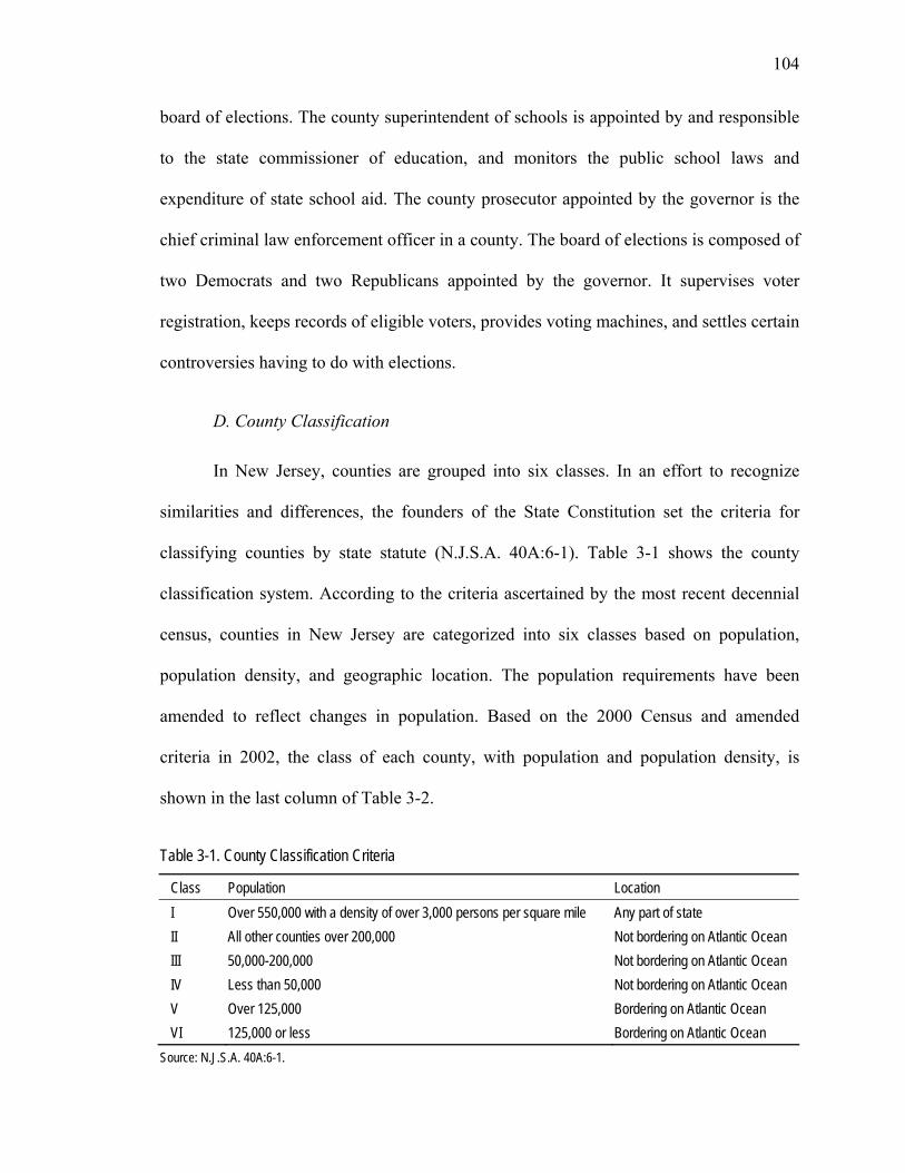
104
board of elections. The county superintendent of schools is appointed by and responsible
to the state commissioner of education, and monitors the public school laws and
expenditure of state school aid. The county prosecutor appointed by the governor is the
chief criminal law enforcement officer in a county. The board of elections is composed of
two Democrats and two Republicans appointed by the governor. It supervises voter
registration, keeps records of eligible voters, provides voting machines, and settles certain
controversies having to do with elections.
D. County Classification
In New Jersey, counties are grouped into six classes. In an effort to recognize
similarities and differences, the founders of the State Constitution set the criteria for
classifying counties by state statute (N.J.S.A. 40A:6-1). Table 3-1 shows the county
classification system. According to the criteria ascertained by the most recent decennial
census, counties in New Jersey are categorized into six classes based on population,
population density, and geographic location. The population requirements have been
amended to reflect changes in population. Based on the 2000 Census and amended
criteria in 2002, the class of each county, with population and population density, is
shown in the last column of Table 3-2.
Table 3-1. County Classification Criteria
Class Population Location I Over 550,000 with a density of over 3,000 persons per square mile Any part of state II All other counties over 200,000 Not bordering on Atlantic Ocean III 50,000-200,000 Not bordering on Atlantic Ocean IV Less than 50,000 Not bordering on Atlantic Ocean V Over 125,000 Bordering on Atlantic Ocean VI 125,000 or less Bordering on Atlantic Ocean
Source: N.J.S.A. 40A:6-1.

105
Table 3-2. Governmental Structure and Classification of the County
Population Population Density Name Form of Government
Elected Officials Land Area
2000 2007 2000 2007
County Classification
Atlantic OCCL-County Executive Plan
County executive 9 Freeholders
561.1 252,552 270,644 450.1 482.4 V
Bergen OCCL-County Executive Plan
County executive 7 Freeholders
234.2 884,118 895,744 3,775.5 3825.2 I
Burlington Board of Chosen Freeholders
5 Freeholders 804.6 423,391 446,817 526.2 555.3 II
Camden Board of Chosen Freeholders
7 Freeholders 222.3 508,932 513,769 2,289.4 2311.2 II
Cape May Board of Chosen Freeholders
5 Freeholders 255.2 102,326 96,422 401.0 377.9 VI
Cumberland Board of Chosen Freeholders
7 Freeholders 489.3 146,438 155,544 299.3 317.9 III
Essex OCCL-County Executive Plan
County executive 9 Freeholders
126.3 792,305 776,087 6,274.8 6146.4 I
Gloucester Board of Chosen Freeholders
7 Freeholders 324.7 254,673 285,753 784.3 880.0 II
Hudson OCCL-County Executive Plan
County executive 9 Freeholders
46.7 608,975 598,160 13,043.6 12812.0 I
Hunterdon Board of Chosen Freeholders
5 Freeholders 429.9 121,989 129,348 283.7 300.8 III
Mercer OCCL-County Executive Plan
County executive 7 Freeholders
225.9 350,761 365,449 1,552.5 1617.5 II
Middlesex Board of Chosen Freeholders
7 Freeholders 309.7 750,162 788,629 2,422.1 2546.3 II
Monmouth Board of Chosen Freeholders
5 Freeholders 471.9 615,301 642,030 1,303.8 1360.4 V
Morris Board of Chosen Freeholders
7 Freeholders 469.0 470,212 488,475 1,002.6 1041.5 II
Ocean Board of Chosen Freeholders
5 Freeholders 636.3 510,916 565,493 803.0 888.8 V
Passaic Board of Chosen Freeholders
7 Freeholders 185.3 490,377 492,115 2,646.5 2655.9 III
Salem Board of Chosen Freeholders
7 Freeholders 337.9 64,285 66,016 190.3 195.4 III
Somerset Board of Chosen Freeholders
5 Freeholders 304.7 297,490 323,552 976.4 1061.9 II
Sussex Board of Chosen Freeholders
5 Freeholders 521.3 144,170 151,478 276.6 290.6 III
Union OCCL-County Executive Plan
9 Freeholders 103.3 522,541 524,658 5,059.0 5079.5 II
Warren Board of Chosen Freeholders
5 Freeholders 357.9 102,433 109,737 286.2 306.6 III
Source: New Jersey Department of Labor and Workforce Development (2000, 2007) - land area, population, and population density; Center for Government Services (2006) - form of government and elected officials.

106
3-1-2. Municipal Governments
Municipalities in New Jersey are independent local government units having
authority to provide many public services immediately consumed by residents such as
police and fire protection, streets, sanitation facilities, and so on. Currently, 566
municipalities operate in New Jersey. In 1930, there were 559 municipalities. Since 1930,
only 10 new municipalities were created and 3 municipalities were eliminated. In 1951,
Landis Township and Vineland City were consolidated into Vineland Township. Loch
Arbour Village, created with the population of 350 in 1957, is the last municipality
created in New Jersey (Karcher, 1998). In 1997, Pahaquarry Township with population
10 was abolished.
New Jersey is the most urbanized and most densely populated of the fifty states.
In terms of population density, New Jersey leads the nation with 1,171 people per square
mile in 2000 and 1,181 people per square mile in 2007 (U.S. Census Bureau, 2007). The
range in population and land area is dramatic. In 2007, the average estimated population
of municipalities was 15,346. While Newark’s estimated population was 280,135,
Teterboro, Pine Valley, and Tavistock had fewer than 30 residents. The average land area
of a municipality is approximately 13.1 square miles. The largest municipality is
Hamilton Township with 111.3 square miles and the smallest municipality is Shrewsbury
Township with 0.09 square miles.
A. Forms of Municipal Government
The differences in the governmental structures are the official positions required,
their method of selection, their powers, and the relationship between the executive and

107
legislative branches. The governmental structures now available to New Jersey
municipalities reflect state statutes enacted at various times during the state’s history.
There are twelve different governmental structures available to New Jersey municipalities.
These twelve distinct governmental structures can be identified by the type of
municipality and the form of government organization.
The type of municipality refers to the official title by which the municipality is
identified: city, town, borough, township, and village. In the past, the type of
municipality was significant in identifying different forms of government under which
the organization of municipalities operated. However, today, all types of municipalities
have basically the same government authority and the type of municipality is merely a
title. The statutes governing those five types of municipalities have been rewritten in
recent years (Reock, 2002). These laws are city form (N.J.S.A. 40:103-5(71) and N.J.S.A.
40A:61-1 et seq.), town form (N.J.S.A. 40A:62-1 et seq.), borough form (N.J.S.A.
40A:60-1 et seq.), township form (N.J.S.A. 40A:63-1 et seq.), and village form (N.J.S.A.
40A:63-8 et seq.).
In addition to the five traditional forms, municipalities can adopt seven optional
forms of government authorized by the laws enacted during the twentieth century. The
first optional form of municipal government was enacted by the legislature in 1911 as the
Commission Form of Government Law (N.J.S.A. 40:70-1 et seq.). In 1923, the
legislature enacted the second optional law, the Municipal Manager Form of Government
Law (N.J.S.A. 40:79-1 et seq.). The third law was the Optional Municipal Charter Law
(OMCL), also known as the Faulkner Act, enacted in 1950. The OMCL provided for four
distinct forms of municipal government: mayor-council form (1950), council-manager

108
form (1950), small municipality form (1950), and mayor-council-administrator form
(1981). Finally, since the revision of the state constitution in 1947, municipalities have
been able to adopt a special charter, which provides for a unique form of government.
The two laws (N.J.S.A. 40:103-5(71) and N.J.S.A. 40A:61-1 et seq.) of the city
form of government provide for a separately elected mayor and council.17 The mayor
serves as chief executive and is the head of the police department, with the power to
appoint senior officers in the police department with the advice and consent of the
council. The mayor has a veto over ordinances. The council is the legislative body and
selects one of its own members to preside as the council president. The council makes
most appointments of municipal personnel with the exception of the police department.
As of January 1, 2005, these two laws were used by only 15 municipalities.
The town form of government (N.J.S.A. 40:63-1 et seq.) provides an elected
mayor for a two or three year term of office and eight council members elected from four
wards for two year overlapping terms. The mayor is the official head of a municipal
government, presides and may vote at council meetings, and has a veto power over
ordinances, which may be overridden only by a two-thirds vote of all members of the
council. The council is the legislative body and makes almost all appointments. All
executive powers not specifically designated for the mayor are exercised by the council.
As of January 1, 2005, only 9 municipalities still used this town form.
The borough form (N.J.S.A. 40A:60-1 et seq.) is the most common among New
Jersey municipalities. This form provides for a mayor and a six member council, elected
17. A series of laws for the city form of government enacted before the early twentieth century have been
repealed. Now, the law of 1963 (N.J.S.A. 40:103-5(71)) allows only East Orange to adopt the city form of government and the law of 1987 (N.J.S.A. 40A:61-1 et seq.) replaced all other city laws (Reock, 2002).

109
separately in partisan elections. The mayor serves for four years, while council members
serve three year staggered terms of office, with two council seats being contested each
year. The mayor presides at council meetings, but votes only to break ties. The mayor
nominates all appointive officers subject to council confirmation. The council has all
executive responsibilities not specifically assigned to the mayor. As of January 1, 2005,
218 municipalities used this borough form.
The township form (N.J.S.A. 40:63-1 et seq.) provides a township committee of
three or five members elected for three year staggered terms. The township committee
exercises all legislative and executive authority of the municipality. Committee members
annually choose one of their own members to serve as mayor for that year. The mayor
presides at committee meetings and votes as a member of the committee, but has no other
special power. In general, all formal legislative and executive powers are exercised by the
committee as a whole. This form is one of the oldest forms of municipal government in
New Jersey and was still used by 144 municipalities as of January 1, 2005.
Under the village form (N.J.S.A. 40A:63-8 et seq.), the governing body is a non-
partisan board of trustees, consisting of five members elected at large for three-year
staggered terms of office. The board of trustees exercises all legislative and executive
authority of the municipality. The president of the board of trustees, who is equivalent to
mayor in other forms of municipal government, is selected from among the five trustees
and serves a one-year term of office. As of January 1, 2005, only Loch Arbour used this
form of government.
The commission form (N.J.S.A. 40:70-1 et seq.) was authorized in 1911. This
form provides for the election of three or five commissioners. The commissioners

110
collectively constitute a board, which is the legislative body of the municipality. The
executive function of the municipality is divided among the three or five commissioners,
each of whom is the director of one of the municipal departments specified by law. One
commissioner is chosen by the board to serve for four years as the mayor and to preside
over meetings of the board. This form of government is used by 32 municipalities as of
January 1, 2005.
The municipal manager form (N.J.S.A. 40:79-1 et seq.) enacted in 1923 is the
second of the major optional laws (Reock, 2002). Under this form of government, voters
elect three, five, or nine members of a council for four-year concurrent terms of office.
The council appoints a municipal manager, a tax assessor, an auditor, a treasurer, a
municipal clerk, and an attorney. Thereafter, the council functions as a legislative body
and administrative duties are prohibited for council members. The mayor is selected by
the council from among its own members, with duties mainly limited to presiding and
voting as a member in council meeting. As of January 1, 2005, only 7 municipalities use
this form of government.
The OMCL mayor-council form (N.J.S.A. 40:69A-1 et seq.) provides for the
election of a council, which is the legislative body of the municipality, and a mayor with
strong executive and administrative powers. The mayor appoints the departmental heads,
the tax assessor, and most members of boards, commissions, and authorities with the
advice and consent of the council. The mayor has a veto power over ordinances, which
may be overridden only by a two-thirds vote of the council. The council, which may
consists of five, seven, or nine members, is limited to legislative functions. The council
selects one of its members to preside, with the title of president of council. Although only

111
67 municipalities had adopted this form of government as of January 1, 2005, they
included most of the large municipalities of New Jersey, including Newark.
Under the OMCL council-manager form (N.J.S.A. 40:69A-1 et seq.), voters elect
five, seven, or nine members of a council for four-year terms of office. The council
appoints most municipal officers, including a manager, a municipal clerk, and a tax
assessor. After appointing the manager, the council is limited to legislative functions and
must act as a body. The manager is the chief executive and either appoints all subordinate
personnel not otherwise provided for or delegates the appointive power to department
heads. The mayor may be selected by the council from among its own members or be
elected directly by the voters. However, the mayor is little more than a presiding officer
for the council. This optional form of government was used by 42 municipalities as of
January 1, 2005.
The OMCL small municipality form (N.J.S.A. 40: 69A-1 et seq.) provides for a
council and a mayor either elected from the council or directly by the voters. The mayor
is the chief executive officer and appoints most municipal officers including an assessor,
a tax collector, a municipal clerk, and a treasurer, with the advice and consent of the
council. The council is the legislative body and has no specified administrative duties or
appointments to make. One member of the council is chosen as the president of the
council to preside in the absence of the mayor. As of January 1, 2005, only 18
municipalities were served by this form of government.
The OMCL mayor-council-administrator form (N.J.S.A. 40:69A-1 et seq.) has
been available by an amendment of the OMCL in 1981. Under this form, a mayor for
four-year terms of office and six members of council for three-year staggered terms of

112
office are elected in at large partisan elections. The mayor appoints most officers
including an administrator, and presides in council meetings, but votes only to break ties.
The mayor also has a veto over ordinances. The administrator is directed to administer
the business affairs and to supervise all of the departments. The council is the legislative
body and members have no administrative duties and no appointive powers. As of
January 1, 2005, only North Brunswick and West Milford used this form of government.
Table 3-3. Forms of Municipal Government in 2005
Land Area (Square Miles)
Population Form of Government Number of Municipality
Total Average Total Average
Average Population Density
Smallest Municipality (Population)
Largest Municipality (Population)
Old Forms
City 15 77.2 5.1 211,409 14,093.9 3,411.7 Corbin City (527)
East Orange (67,508)
Town 9 65.4 7.3 124,670 13,852.2 9,928.3 Clinton Town (2,588)
Kearny (38,707)
Borough 218 550.6 2.5 1,533,911 7,036.2 3,815.6 Rockleigh (393)
Sayreville (42,744)
Township 144 4,083.6 28.4 1,584,717 11,005.0 894.6 Walpack (40)
Lakewood (68,688)
Village 1 0.1 0.1 279 279.0 2,883.7 Loch Arbour (279)
Loch Arbour (279)
Optional Forms
Commission 32 167.4 5.2 363,600 11,362.5 6,332.7 Pine Valley (22)
Union City (65,021)
Municipal Manager (1923)
7 23.6 3.4 196,836 28,119.4 8,176.2 Teterboro (18)
Clifton (78,911)
OMCL: Mayor-Council 67 1,200.8 17.9 3,170,671 47,323.5 5,067.5 Avalon (2,188)
Newark (277,903)
OMCL: Council-Manager
42 771.4 18.4 975,170 23,218.3 2,915.2 Springfield (3,528)
Franklin TWP (57,921)
OMCL: Small Municipality
18 261.2 14.5 132,959 7,386.6 2,158.4 Estell Manor (1,708)
Stafford (25,522)
OMCL: Mayor-Council- Administrator
2 87.5 43.7 67,254 33,627.0 1,824.2 West Milford (27,825)
North Brunswick (39,429)
Special Charters 11 128.5 11.7 295,969 26,906.3 4,147.3 Hardyston (7,797)
Middletown (67,224)
Total /Average 566 6,866.7 13.1 8,657,445 15295.8 3,381.6
Source: New Jersey Department of Labor and Workforce Development (2005) - land area, estimated population, and population density; Center for Government Services (2006) - form of government.

113
The special charter provides a unique form of governmental organization for
municipalities through the enactment of a law providing them with their own special
charter. The special charter approach has been available for municipalities since the state
revised its constitution in 1947. 18 This special charter procedure has become more
popular in recent years. Through this special charter, municipalities usually have adopted
a unique variation of existing optional forms of government to meet the desires of a
particular community. As of January 1, 2005, 11 municipalities operated under special
charters.
Table 3-3 reports the number of municipalities and demographics by the form of
governmental organization, which is reviewed above. The most recent published data on
the form of municipal government is the year 2005 and, thus, the table is constructed
based on the form of government in 2005.
B. Classification of Forms of Municipal Government
Although municipalities in New Jersey operate under 12 different forms of
governmental organization, they can be categorized into the three general types based on
the powers of and relationships between executive and legislative authorities: 1) elected
governing body and elected chief executive, 2) elected governing body and appointed
chief executive, and 3) elected governing body-administrators (Braun, 2002; Reock,
2002). Table 3-4 shows how 12 different forms of government, which are now available
by state laws in New Jersey, fit into the three broad patterns of municipal government.19
18. The special charter was prohibited from 1875 through 1947 by an amendment of the State Constitution
(Reock, 2002). 19. Exceptions are 11 municipalities adopting special charters. Because these municipalities are operated under
different variations of existing optional forms, they cannot be classified as a whole into any one of the above three categories.

114
In the elected governing body and elected chief executive pattern, there is a
directly elected chief executive, usually called the mayor, and a separately elected
legislative body, usually called the council. This pattern is similar to the organizational
structure of the federal and state governments in that each chief executive and the
legislative body has powers serving as a check on any abuse of the other. The mayor has
most executive powers and the council is usually limited to legislative functions. As of
January 1, 2005, 329 municipalities could be categorized into this general pattern of
municipal government. These municipalities are operated under one of city, town,
borough, mayor-council, small municipality, and mayor-council-administrator forms.
The elected governing body and appointed chief executive pattern resembles the
forms of private firms. Under this pattern, voters elect members of the governing body
that appoints a chief executive. After appointing the chief executive, usually called the
manager or administrator, the governing body is limited to the legislative function and the
administrative power is delegated to the appointed chief executive. The mayor may be
selected by the council from among its own members or be elected directly by the voters,
with duties limited to presiding over the council. As of January 1, 2005, 49 municipalities
operated under the municipal manager (1923) and the council-manager forms could be
categorized into this pattern.
The elected governing body-administrator pattern is government by committee.
Under this pattern, voters elect members of the governing body who serve both as the
chief executive and as the legislative body. In practice, the legislative powers are usually
exercised by the governing body as a whole, while the executive powers are divided
among the individual members of the governing body, with each member specializing in

115
some aspect of municipal government. The governing body selects one of their own
members as the mayor. As of January 1, 2005, the 176 municipalities using township,
village, and commission forms of government could be considered as falling into this
pattern of government.
Table 3-4. Forms of Municipal Government by General Pattern of Organization in 2005
Elected Governing Body & Elected Chief
Executive
Elected Governing Body & Appointed Chief
Executive
Elected Governing Body-Administrators
Old Forms
City 15
Town 9
Borough 218
Township 144
Village Form 1
Optional Forms
Commission 32
Municipal Manager (1923) 7
OMCL: Mayor-Council 67
OMCL: Council-Manager 42
OMCL: Small Municipality 18
OMCL: Mayor-Council Administrator 2
Special Charters Mixed - 11
Total Number of Municipality 329 49 177
Source: Center for Government Services (2006).
3-1-3. School Districts
In New Jersey, the state government and the local school district are responsible
for providing public education services. Under the State Constitution, every child
between the ages of five and eighteen years is entitled to receive a “thorough and

116
efficient” education. The constitution holds the state responsible for achieving the
“thorough and efficient” education.
A. Overview of Elementary and Secondary Education
At the state level, the primary administrative authorities for elementary and
secondary education are the State Board of Education and the Department of Education.
The major function of the State Board of Education is the consideration and adoption of
administrative codes, which contain the rules for implementing education laws. The
Department of Education enforces the rules and regulations established by the state board.
In addition, the Department of Education supervises all schools receiving state funds,
apportions school aid and certifies payments, and sets forth minimum standards of study
for schools.
At the local level, the local school district is the governmental unit charged with
the responsibility for providing public education. In fact, while the state constitution
assigns responsibility for education to state government, the state government assigns or
delegates most provision of primary and secondary education services to local school
districts. To ensure the goal of public education set by state constitution and statutes and
to implement the broad education policies set by state government, local school districts
superintend and manage the schools; adopt rules for their organization, government, and
instruction; and prescribe textbooks and courses of study.
Statistics on schools, enrollments, and education expenditures indicate the
growing importance of public education and, thus, the role of local school districts in
providing education services. According to New Jersey Vital Education Statistics, which

117
is annually published by the NJ DOE, the number of public school enrollments and the
number of public schools grew steadily during the period from 2000 through 2005. The
total number of public schools rose from 2,363 to 2,422. Enrollments in elementary
school rose from 934,502.5 to 956,299 and enrollment in secondary school from
378,891.5 to 437,482.
The cost of public elementary and secondary education is shared among the
federal government, the state government, and the property taxpayers of the local school
district. As we will see in Table 3-12, in New Jersey, the largest amount of education
expenditures is financed by local property taxes, constituting over 60% of total spending
for education. State contribution to education expenditure follows behind the local
government with about 40% of total education expenditure. The federal share is very
small and is omitted in the analysis due to lack of data. The statistics indicates that,
although the state government has increased its role in education, the school district is
still the main governmental unit in providing public elementary and secondary education.
Table 3-5. Public Schools and Enrollments (2000-2005)
Starting School Year 2005 2004 2003 2002 2001 2000
Schools
Total 2,422 2,413 2,398 2,384 2,381 2,363
Elementary 1,943 1,936 1,926 1,911 1,906 1,890
Secondary 398 398 391 390 389 386
Handicapped 81 79 81 83 86 87
Enrollments
Total 1,393,781.5 1,391,169.5 1380,881.5 1,367,289.5 1,341,503.0 1,313,394.0
Elementary 956,299.5 961,321.0 960,143.0 959,155.0 950,703.5 934,502.5
Secondary 437,482.0 429,848.5 420,738.5 408,134.5 390,799.5 378,891.5
Source: NJ DOE (2007). Notes: Students can attend public school full time or attend two schools on a shared-time basis. Full time student are reported as 1 and shared-time students are reported as 0.5 at each school.

118
B. Local School Districts
With development of public education as a governmental activity in the 19th
century, school districts were created in New Jersey (Benecke, 2004a). As of October 15,
2007, there were a total of 616 local school districts in New Jersey. These local school
districts are independent local governmental units established to provide public education
services to their residents. Although local school districts are regulated by the federal and
state governments, they can implement any policy as long as it does not violate the
federal or state statutes and regulations.
Local school districts can be classified by several criteria such as the type of
operation, the authority to tax, the jurisdiction, and the structure of the governing body
authorized by the state education law. These classifications are useful in understanding
the function of the school district and its relation to other local governmental units,
especially municipalities. Table 3-6 provides the total number of school districts and the
number of school districts by type, and these figures are almost constant during the
period from 2000 through 2007.
By the operation type, there were 593 operating and 23 non-operating school
districts as of October 15, 2007. The non-operating school district has been established
legally with a board of education, but does not operate any schools. Considering the
power to tax, school districts are classified into 574 fiscally independent school districts
having authority to tax and 42 school districts having no power to tax. The 42 school
districts without power to tax include 21 county vocational school districts, 8 county
special service school districts, and 12 educational services commissions.

119
The county vocational school district may be established by the county board of
chosen freeholders or by referendum for vocational education. The county special
services school district is established by the county board of chosen freeholders for the
education of handicapped children. The educational services commission is a public, non-
profit organization which provides educational programs for its constituent school
districts.
The 574 fiscally independent school districts provide elementary and secondary
education. Based on their jurisdictions, these fiscally independent school districts can be
further classified into regular school districts, and regional or consolidated school
districts. While regular school districts have the same geographic boundaries as
municipalities, 70 regional and 8 consolidated school districts serve more than one
municipal area.
Table 3-6. Number of School Districts (2000-2007)
Starting School Year 2007 2006 2005 2004 2003 2002 2001 2000
Total 616 615 615 616 616 616 615 616
By Operating Type
Operating 593 592 592 593 593 593 592 593
Non-Operating 23 23 23 23 23 23 23 23
By Budget Type
Independent 574 574 574 574 574 574 574 575
Regular 496 496 496 496 496 496 495 496
Regional 70 70 70 70 70 70 71 71
Consolidated 8 8 8 8 8 8 8 8
County Vocational 21 21 21 21 21 21 21 21
Others 21 20 20 21 21 21 20 20
Source: Center for Government Services (2001-2006) – statistics by budget type; NJ DOE (2007) - total statistics and statistics by operation type. Notes: Others include county special service school districts and educational services commissions.

120
Regional school districts are formed when two or more school districts combine
for a limited purpose as in establishing a Kindergarten through grade 12 or a grade 9
through grade 12 school district (NJ DOE, 2007). Consolidated school districts are
formed through the merger of two or more existing municipalities into a single school
district. In New Jersey, school district jurisdictions are always coterminous with
municipal boundary or boundaries. This means that although the regional or the
consolidated school districts govern more than one municipal jurisdiction, they do not
encompass less than the total area of one municipality.
C. Legal Classification of Local School Districts
The New Jersey state education law (N.J.S.A.18A:9-2 to 3) classifies local school
districts as either Type I or Type II school districts. As of October 15, 2005, among 574
independent school districts, there were 20 Type I school districts and all other
independent school districts were classified as Type II school districts, with the
exceptions of 3 school districts operated by the state government. Those 3 state operated
school districts are Newark, Jersey City, and Paterson school districts. All regional and
consolidated school districts are classified as Type II school districts.
The state education law (N.J.S.A.18A:9-4 to 6) allows voters of a school district
to change the Type of school district through a referendum at the annual school election.
The process can be initiated either by a resolution of the municipal governing body in
Type I school districts, by a resolution of the board of education in Type II school
districts, or by a petition signed by 15% of the number of voters who voted in the last
general election at which all members of the general assembly were elected.

121
Between the Type I and the Type II school district, there are critical differences in
the selection method of board of education members, the power of the education board,
and the relationship between the school district and the municipal government. These
differences are summarized in Table 3-7.
Table 3-7. Characteristics of Type I and II School Districts
Type I Type II
School Board Appointed by the mayor Elected by the voter
Budget Approval By the board of school estimate By the municipal governing body where the tax rate exceeds $1.5 per $100 assessed valuation
By the voter
Bond Issue Approval The board of school estimate The municipal governing body
By the voter
Election No Annual election
Source: Benecke (2004a)
D. Board of Education
The local school district is governed by the board of education. The members of
the education board are local education policy-makers. While the state government
establishes the broader framework within which school districts must operate, the board
of education sets many of the policies and procedures that most directly affect students
and school staffs. The board of education members meet regularly to discuss personnel,
finance, curriculum, and other relevant issues. The size of the local board of education
may be three, five, seven, nine, or eleven members.
The selection method of board of education members differs by the legal type of
school district. While the board of education members are appointed by the mayor in
Type I school districts, voters elect education board members for three-year staggered

122
terms in Type II school districts. In the Type II regional or consolidated school districts,
the number of board of education members is apportioned among the member school
districts participating in the regional or consolidated school district according to the
population of the member school districts. The voters within each member school district
elect the apportioned education board members.
One of the most important duties of the board of education is to determine the
amount of money to be raised by local property taxes for schools and school bond
issuance to finance any capital projects. This annual budget process of school districts is
quite different between the Type I and Type II school districts.
In a Type I school district, the annual budget is prepared by the board of
education and is submitted for approval to the board of school estimate, which consists of
the mayor, two members of the school board, and two members of the municipal
governing body (Benecke, 2004a). School debt and the amount to be raised by property
tax must be included in the official municipal budget. School debt is considered part of
the municipality’s responsibility to the extent that the municipal governing body must
directly appropriate the capital funds. However, school debt service is raised as part of
the property tax allocated for schools.
In a Type II school district, the annual budget of the school district is also
established by the board of education. However, unlike the Type I school district, the
school tax levy and school debt are submitted for voter approval in a school district
election (Benecke, 2004a). School debt is an obligation of the school district alone, rather
than of the municipality. The budget of Type II consolidated or regional school districts
must be submitted to the voters of the member school districts for approval.

123
The board of education has the power to appoint school district personnel such as
the superintendent of schools, the school business administrator, and the board secretary,
among others (Benecke, 2004a). The superintendent of schools is the chief administrative
officer of the school district. The duties of the superintendent include almost all activities
of the school district such as maintaining the quality of educational programs and
services, directing and supervising the administrative staff, initiating and supervising
development of the annual budget, and overseeing school facility management (N.J.S.A.
18A:17-15).
The school district’s staff includes a school board secretary. In addition, the
position of business administrator may be established as a separate position (Benecke,
2004a). In many school districts, the business administrator also serves as the education
board secretary. The business administrator is generally responsible for the day-to-day
administrative operations of the school district, including purchasing, budget control,
payroll processing and general control of cash receipts and disbursements (N.J.S.A.
18A:17-14.1).
Another financial officer of the school district is the treasurer of school monies.
This is a statutory position assigned to the treasurer of the municipality, unless the board
of education designates the tax collector or clerk (N.J.S.A.18A:17-31 to 36). The basic
duties of the treasurer are to reconcile and certify the receipts and disbursements of the
school district. In regional or consolidated school districts containing more than one
municipality, the treasurer comes from the constituent municipality which has the largest
amount of taxable property value (Benecke, 2004a).

124
3-1-4. Other Local Governmental Entities
In New Jersey, state law authorized local governmental units other than counties,
municipalities, and school districts, to be also able to provide public services. With
sufficient administrative and fiscal autonomy to qualify as separate governmental units,
these local governmental units perform a single or a limited number of functions. Based
on power to tax and independence from counties or municipalities, these local
governmental units can be classified into a special district, a self-liquidating municipal
utility, and a public authority. Table 3-8 provides the total number of and property taxes
for special districts for the years 1993, 2004, and 2005.20
A. Special Districts
In New Jersey, special districts were originally developed to provide public
services to unincorporated areas or sparsely populated rural areas not served by any local
or state government. Counties and municipalities can create special districts to perform
specific functions within their jurisdictions. Special districts are generally autonomous
with their own power to tax, impose service charges, and issue bonds, and their officials
are usually elected (Benecke, 2004a).
The typical service areas of special districts are fire, garbage, sewerage, water,
and business improvement. The service is provided to the entire region or to a
geographical area of a local government jurisdiction. Thus, several special districts
providing the same service may exist within a local government jurisdiction. The annual
budget of special districts, including the property tax levy, is determined by their elected
20. Same data for self-liquidating municipal utilities and public authorities are not available.

125
governing body or by the local government governing body. The special district budget is
subject to approval by voters or by the local government governing body.
Table 3-8. Number of Special Districts in New Jersey
Year Total Fire Special Improvement Garbage/Solid Waste Water Light Total Tax Levy ($)
2005 238 193 32 12 1 0 198,865,404
2004 237 192 31 12 2 0 184,371,768
1993 244 201 4 15 2 22 107,550,000
Source: NJ DLGS (1994) – 1993 data; NJ DLGS (2004-05) – 2004-05 data.
B. Self-Liquidating Utilities
A self-liquidating municipal utility is a governmental entity created to perform a
specific function or functions within a local government jurisdiction or region (Benecke,
2004a). The self-liquidating utility provides numerous public services such as water,
sewer, harbor, electric, and solid waste. Unlike special districts, the self-liquidating utility
is not independent from local governments since the governing body of the local
government is responsible for the budget and operations of the self-liquidating municipal
utility. The annual budget of a self-liquidating utility is included in the municipal budget
as a required separate section. The main revenue for financing operation costs, debt
service, and capital spending comes from user fees and charges.
C. Public Authorities
A public authority is a corporate public entity created by local governments to
provide specific services within a local unit or region. New Jersey local governments
have extensively utilized the public authority (Benecke, 2004a). The public authority can
be characterized as quasi-public in that it performs a public function without power to tax.

126
Public authorities provide specific services, such as landfill disposal, sewerage processing,
and water delivery. The public authority and the municipality normally enter into a
service agreement which establishes the terms and conditions under which the services
are delivered.
3-2. Expenditures and Revenues of Local Governments
In New Jersey, counties, municipalities, school districts, and other special districts
are operating to provide local public services and goods. This section describes what
services these local governments provide and how they are financed. First, this section
provides a brief overview of the local government budget process: what is the budget,
who is responsible for the budget, and how the budget process is controlled. Second, this
section provides a profile of expenditures and revenues by state and local governments.
3-2-1. Local Government Budget Process
The two major policy decisions to be made by local governments are the level of
public services to be provided and the amount of money to be raised for financing these
public services. These two policy decisions are made through the annual budget process.
A budget is a financial plan involving the two policy decisions: the estimate of
expenditures for public services and the proposed method of financing these expenditures
through various revenue sources. The local government budget constitutes two functions
of authority. First, it establishes the appropriations necessary to meet the estimated
expenditures (Benecke, 2004a). Second, it provides the power to tax to provide the
revenue needed to bring the budget into balance (Benecke, 2004a). Since it must be
adopted annually, the budget is the most important action of local governments.

127
In New Jersey, although no law requires the governing body of a local
government to actually prepare the budget, the governing body officials usually involve
themselves deeply either as individuals or through committees in the administrative
aspects of budget decisions (Benecke, 2004b). Through the annual budgetary process, the
governing body of the local government establishes appropriations for specific funding
units such as police, fire, and public works, and identifies sources of revenues to fund the
expenditure. In addition, the governing bodies of all local governments are responsible
for the final adoption of the budget (Benecke, 2004a). The governing body can amend the
budget prior to the time of holding the public hearing and during or after the public
hearing.
In New Jersey, local government budgets are subject to state laws and are
supervised by the state government. Municipalities and counties must comply with the
provisions of the Local Budget Law (N.J.S.A. 40A:4-1 et seq.) and school districts must
comply with the provisions of the Comprehensive Educational Improvement and
Financing Act of 1996 (CEIFA). These laws prescribe the timing, general content,
required local government governing body action, and other important aspects of the
local government budget process. The Local Budget Law also requires that a formal
public hearing be held prior to the final adoption of the local budget. This allows public
input and discussion prior to the budget being adopted. Citizens may play an important
role either in reviewing and supporting proposed budgets, or even in providing input to
the structure of the budget.
The local budget process is also controlled by the state government. Budgeting,
accounting, and auditing are controlled by the Division of Local Government Services in

128
the Department of Community Affairs for counties and municipalities and by the
Department of Education for school districts. The Division of Local Government
Services and the Department of Education establish procedures and regulations which
local governments are required to adhere to under uniform budgetary forms. In addition,
the Division of Taxation in the Department of Treasury is responsible for the supervision
of property tax assessment at the municipal, county, and state levels. The director of the
Division of Taxation has the statutory responsibility for supervision and coordination of
local property tax assessment and tax procedures.
3-2-2. Expenditures of Local Governments
In New Jersey, the state and local governments share responsibility, at least to
some extent, for delivering most public services. The assignment of service
responsibilities among the state and the local governments can be based on provisions of
state constitution and statutes. However, it is a daunting task to identify the service
responsibility through examining state constitutional and statutory provisions. Data on
expenditures by state and local governments can provide some evidence on the
assignment of service responsibilities among the state and local governments.
Classifying government expenditure is important in identifying the relative role in
providing various public services through government expenditures. Government
expenditures can be grouped by several criteria such as accounting or object, government
function, program or project, executing agency or entity, and so on. A classification by
function is most widely used and is useful in analyzing the service responsibilities. The
U.S. Census Bureau’s data on state and local government finances, in which government

129
expenditures are classified based on government function, is used to review the functions
of state and local governments. 21
Table 3-9 shows expenditures of state and local governments by function with the
percentage of each category and state and local shares in each category. It provides some
perspective on the relative importance of these various government activities by total and
by levels of government. The table reveals that education, social service, and public
safety are the three largest components of state-local government spending. Education,
social service, and public safety expenditures constitute about 34%, 18%, and 7.5 %,
respectively, of all dollars spent by state and local governments.
The importance of government functions differs by state and local governments.
State government is the predominant provider of social service, transportation, and utility
services. Social service expenditure of state government represents about 25% of state
total expenditure and about 90% of total social expenditure by state and local
governments. Although education is the second largest component of state expenditure
(about 13%), the state’s portion is slightly over 24% of total education spending by state
and local governments. 22 On the other hand, although transportation and utility
expenditures take only about 4 % each of total state spending, the state’s proportion of
total state-local spending on these two services is about 62% and 71%, respectively.23
21. According to the U.S. Census Bureau’s data on state and local government finances, local government
expenditures are classified into followings: education - higher education, elementary and secondary education, and libraries; social service - public welfare, hospitals, and health; transportation - highways, airports, parking, and port facilities; public safety - police, fire, and correction; environment and housing - natural resources, parks and recreation, housing, sewerage, and solid waste; governmental administration - financial judicial and legal, and general public buildings; public utility - water, electric power, gas, and transit; and others - interest on debt, insurance trust, and other expenditures.
22. State government is responsible for the higher education and its share of total higher education expenditure is about 80%.
23. Capital expenditure takes over 50% of state’s transportation expenditure and transit service expenditure represents over 95% of state’s utility expenditure.

130
Table 3-9. State and Local Government Expenditure by Functions (2003-04 ~ 2005-06)
Year 2005-06 2004-05 2003-04 Total* State Local* Total* State Local* Total* State Local*
Total Expenditure* 82,928,181 54,073,301 40,193,729 79,845,099 50,964,235 39,835,246 74,335,925 48,975,600 36,220,682
Intergovernmental 49,906 11,060,423 328,332 0 10,642,426 311,956 0 10,565,755 294,602Expenditure* (0.1%) (20.5%) (0.8%) (0.0%) (20.9%) (0.8%) (0.0%) (21.6%) (0.8%)
Direct Expenditure 82,878,275 43,012,878 39,865,397 79,845,099 40,321,809 39,523,290 74,335,925 38,409,845 35,926,080 (99.9%) (79.5%) (99.2%) (100.0%) (79.1%) (99.2%) (100.0%) (78.4%) (99.2%)
(51.9%) (48.1%) (50.5%) (49.5%) (51.7%) (48.3%)
Education 28,167,152 7,019,789 21,147,363 26,987,883 6,648,228 20,339,655 24,999,848 6,104,928 18,894,920 (34.0%) (13.0%) (52.6%) (33.8%) (13.0%) (51.1%) (33.6%) (12.5%) (52.2%)
(24.9%) (75.1%) (24.6%) (75.4%) (24.4%) (75.6%)
Social Services 15,448,620 13,897,075 1,551,545 14,397,828 12,892,200 1,505,628 13,142,527 11,741,334 1,401,193 (18.6%) (25.7%) (3.9%) (18.0%) (25.3%) (3.8%) (17.7%) (24.0%) (3.9%)
(90.0%) (10.0%) (89.5%) (10.5%) (89.3%) (10.7%)
Transportation 3,718,034 2,427,531 1,290,503 3,267,356 2,002,806 1,264,550 3,266,628 2,071,976 1,194,652 (4.5%) (4.5%) (3.2%) (4.1%) (3.9%) (3.2%) (4.4%) (4.2%) (3.3%)
(65.3%) (34.7%) (61.3%) (38.7%) (63.4%) (36.6%)
Public Safety 6,225,551 2,179,658 4,045,893 5,884,360 2,064,519 3,819,841 5,528,681 1,905,866 3,622,815 (7.5%) (4.0%) (10.1%) (7.4%) (4.1%) (9.6%) (7.4%) (3.9%) (10.0%)
(35.0%) (65.0%) (35.1%) (64.9%) (34.5%) (65.5%)
Environment & 4,786,984 1,291,053 3,495,931 5,913,550 1,082,706 4,830,844 4,302,620 984,675 3,317,945Housing (5.8%) (2.4%) (8.7%) (7.4%) (2.1%) (12.1%) (5.8%) (2.0%) (9.2%)
(27.0%) (73.0%) (18.3%) (81.7%) (22.9%) (77.1%)
Governmental 3,262,755 1,707,866 1,554,889 3,183,702 1,633,219 1,550,483 3,054,388 1,554,208 1,500,180Administration (3.9%) (3.2%) (3.9%) (4.0%) (3.2%) (3.9%) (4.1%) (3.2%) (4.1%)
(52.3%) (47.7%) (51.3%) (48.7%) (50.9%) (49.1%)
Utility 3,297,597 2,334,865 962,732 3,256,054 2,302,798 953,256 3,202,453 2,259,558 942,895 (4.0%) (4.3%) (2.4%) (4.1%) (4.5%) (2.4%) (4.3%) (4.6%) (2.6%)
(70.8%) (29.2%) (70.7%) (29.3%) (70.6%) (29.4%)
Others 17,971,582 12,155,041 5,816,541 16,954,366 11,695,333 5,259,033 16,838,780 11,787,300 5,051,480 (21.7%) (22.5%) (14.5%) (21.2%) (22.9%) (13.2%) (22.7%) (24.1%) (13.9%)
(67.6%) (32.4%) (69.0%) (31.0%) (70.0%) (30.0%)
Source: U.S. Census Bureau (2003-04 ~ 2005-06). Notes: 1. Dollar amounts are in thousands. 2. Local government figures are the sum of expenditures of counties, municipalities, school districts, and other special districts. 3. * Duplicative intergovernmental transactions are excluded. 4. The second and the third row of each expenditure category represent the percentage of each expenditure category to the total expenditure and the proportion of state and local governments combined in the expenditure category, respectively.
The major financing responsibilities of local governments are education, public
safety, and environment and housing services. 24 Education expenditure accounts for
24. Housing is primarily a private sector activity. However, some housing is provided by the public sector, with
local governments generally taking the lead role.

131
about 52% of total local government expenditures and slightly more than 75% of total
state-local expenditure on education. Local governments are primarily responsible for
elementary and secondary education, and contribute about 90% of total expenditure on
this category.25 While local government expenditures on public safety and environment
and housing are the second and third largest components, each represents only 10% of
total local spending. However, local governments finance over 70% of total state-local
expenditures on environment and housing services and about 65% of state-local
expenditure on public safety. The responsibility of local governments with lowest
expenditure is social services, contributing only about 10% of total state-local social
expenditures.
A basic understanding of local government fiscal behavior requires detailed
information on the amounts spent by each type of local government. Table 3-10 compares
total expenditures by type of local government for the period from 2004 through 2007
with the percentage change and the percentage which each type of government represents
of the aggregate.26 The growth in expenditures by local government in New Jersey during
the period is clear. Local governments spent 34.36 billion dollars in 2004 and the total
expenditure had increased 16.3% by 2007. During the period, counties, municipalities,
and school districts annually increased their expenditures by 6.0%, 6.2%, and 4.9%,
respectively.
In the relative importance by the type of government, school districts report the
largest expenditure during the period, constituting about 57% of the total local
25. Local government expenditures on this category include state aid to school districts. 26. The total local government expenditure in Table 3-10 is smaller than that in Table 3-9 because expenditures
of special districts are dropped in Table 3-10 due to lack of data.

132
expenditure. Municipalities and counties follow with 28% and 14%, respectively. The
share of each government also has been changed. While school districts’ share decreased
from 58.2% to 57.4%, municipalities’ and counties’ increased from 27.4% to 28% and
14.3% to 14.5%, respectively. Although the period examined here covers a short duration
of time, these shifts may reflect both changes in service demands and changes in the
system for delivering local public services. It may also reflect shifts in available revenues,
particularly regarding intergovernmental aid from state government.
Table 3-10. Local Government Spending by the Type of Local Government (2004-2007)
Year 2007 2006 2005 2004
Total 39.94 38.20 36.35 34.36 (4.6%) (5.1%) (5.8%)
County 5.81 5.49 5.20 4.92 (5.8%) (5.6%) (5.7%) (14.5%) (14.4%) (14.3%) (14.3%)
Municipality 11.19 10.62 10.08 9.43 (5.4%) (5.4%) (6.9%) (28.0%) (27.8%) (27.7%) (27.4%)
School District 22.94 22.09 21.07 20.01 (3.8%) (4.8%) (5.3%) (57.4%) (57.8%) (58.0%) (58.2%)
Source: NJ DLGS (2000-2007a). Notes: 1. Dollar amounts are in Billions. 2. The second and the third rows of each type of local government represent annual change and each type of local government’s share of total expenditure, respectively.
3-2-3. Revenues of Local Governments
An essential part of the government budget is the revenue section indicating the
amount of revenue by sources, which is required for financing various public services.
State and local governments are required to raise a substantial portion of their revenues
using their own taxing and charging powers. The major revenue items in the

133
government’s annual budget include tax revenues, user charges and fees,
intergovernmental transfers form other levels of government, and other miscellaneous
revenues. Table 3-11 shows revenues of state and local government by source with the
percentage of each revenue source during the period from fiscal year 2003-04 through the
2005-06 fiscal year. In addition, it also reports state and local shares in each revenue
category.
Taxes are the main source of state-local revenues and represent over 52% of total
state-local revenues. The main tax instruments for state and local governments in New
Jersey are property, sales, and income taxes. The second largest amount of revenue
comes from user charges and fees, which contribute almost 17% of total state-local
revenues. Other miscellaneous revenues follow with approximately 15% of total state-
local revenues. These own sources for revenues represent over 85% of total state-local
revenues. The remaining revenue comes from intergovernmental transfers from other
levels of governments.
If state and local governments are looked at separately, the relative importance of
each revenue source differs by state and local governments. The data reveals that taxes
constitute about 40% of total state revenues and slightly more than 50% of total local
government revenues. State government depends heavily on sales taxes and income taxes.
Income taxes constitute more than 20% of total state revenues and are used exclusively
for state government. Revenue from sales tax is the next major state government source
of revenue. Sales tax contributes nearly as much as income tax to the total state revenue
(almost 19%). Although local governments are also allowed to levy sales tax, it generates
an almost negligible amount of local revenue (about 0.2%). On the other hand, a primary

134
revenue source for local governments is the property tax. Local governments rely heavily
on property taxes, which constitute more than 50% of total local government revenue.
The second largest revenue for state and local government comes from various
charges and fees for the use of many public services. The state government relies for
about 15% of total state revenues on user charges and fees for public services provided,
especially on fees and charges for highway, hospital, and higher education usage. User
charges and fees also represent approximately 14% of total local revenues and usually
come from sewerage and solid waste, and higher education services. Finally, state and
local governments earn other miscellaneous types of revenue from charges for use of
public utilities and interest. The state government raises about 19% of state revenue from
other miscellaneous revenues, which include user charges for the use of public transit
service and interest earned on cash balances deposited in interest-earning accounts. Local
governments, on the other hand, rely for slightly over 2% of total local revenues on this
revenue category. Local miscellaneous revenue comes mainly from charges for water
service.
In addition to their own sources of revenues mentioned above, state and local
governments rely for a considerable proportion of their revenue on intergovernmental
transfers. About 19% of state government revenue is derived from transfers from other
levels of governments. Local governments receive more than 30% of total local revenue
from transfers from other levels of government, especially the state government.
Whatever the cause, New Jersey was ranked first in property tax per capita in 2006 (Tax
Foundation, 2008). In 2002, as a share of state-local revenues and as a share of local
revenues, New Jersey was ranked in the top five states (U.S. Census Bureau, 2002;

135
Regional Plan Association, 2005). To relieve the property tax burden of residents and
reduce local governments’ reliance on property taxes, the state government plays an
important role in financing local government mainly by channeling money to the local
governments through state aid programs. While the Department of Education allocates
state aid funds to school districts, state aid to counties and municipalities is governed
mainly by the Department of Community Affairs. Some state aid to local governments is
formula based while others are provided through competitive grants.
Table 3-11. State and Local Government Revenues by Source in New Jersey (2003-04 ~ 2005-06)
Year 2005-06 2004-05 2003-04 Total* State Local* Total* State Local* Total* State Local*
Total* 85,516,847 57,610,331 39,887,281 79,125,811 52,661,668 38,303,150 75,527,008 51,041,285 35,658,032
Intergovernmental 11,746,301 11,378,454 12,348,612 10,626,825 10,258,349 12,207,483 10,163,630 9,815,674 11,520,265 Revenue* (13.7%) (19.8%) (31.0%) (13.4%) (19.5%) (31.9%) (13.5%) (19.2%) (32.3%)
Taxes 47,307,677 26,266,187 21,041,490 43,871,003 24,247,648 19,623,355 39,558,277 20,986,204 18,572,073 (55.3%) (45.6%) (52.8%) (55.4%) (46.0%) (51.2%) (52.4%) (41.1%) (52.1%)
Property 20,549,427 3,479 20,545,948 19,196,599 3,484 19,193,115 18,229,254 3,660 18,225,594 (24.0%) (0.0%) (51.5%) (24.3%) (0.0%) (50.1%) (24.1%) (0.0%) (51.1%)
(0.02%) (99.98%) (0.02%) (99.98%) (0.02%) (99.98%)
Sales 10,608,212 10,493,283 114,929 10,238,453 10,171,999 66,454 9,780,318 9,740,284 40,034 (12.4%) (18.2%) (0.3%) (12.9%) (19.3%) (0.2%) (12.9%) (19.1%) (0.1%)
(98.9%) (1.1%) (99.4%) (0.6%) (99.6%) (0.4%)
Income 13,014,993 13,014,993 0 11,762,572 11,762,572 0 9,297,731 9,297,731 0 (15.2%) (22.6%) (0.0%) (14.9%) (22.3%) (0.0%) (12.3%) (18.2%) (0.0%)
(100.0%) (0.0%) (100.0%) (0.0%) (100.0%) (0.0%)
Other Taxes 3,135,045 2,754,432 380,613 2,673,379 2,309,593 363,786 2,250,974 1,944,529 306,445 (3.7%) (4.8%) (1.0%) (3.4%) (4.4%) (0.9%) (3.0%) (3.8%) (0.9%)
Charges and Fees 14,333,873 8,801,264 5,532,609 13,254,239 7,678,085 5,576,154 12,315,192 7,554,939 4,760,253 (16.8%) (15.3%) (13.9%) (16.8%) (14.6%) (14.6%) (16.3%) (14.8%) (13.3%)
Others 12,128,996 11,164,426 964,570 11,373,744 10,477,586 896,158 13,489,909 12,684,468 805,441 (14.2%) (19.4%) (2.4%) (14.4%) (19.9%) (2.3%) (17.9%) (24.9%) (2.3%)
Source: U.S. Census Bureau (2003-04 ~ 2005-06). Notes: 1. Dollar amounts are in thousands. 2. Local government figures are the sum of revenues of counties, municipalities, school districts, and other special districts. 3. * Duplicative intergovernmental transactions are excluded. 4. The second row of each revenue source represents its share of total revenues, and the third row in property, sales, and income taxes provides the proportion of state and local governments.

136
While local governments, as combined, derive a considerable portion of their
revenues from property taxes, user charges and fees, and state aid, the reliance on each of
these revenue sources may differ by the type of local government. Table 3-12 shows the
amount and contribution of each source of revenue to total revenue by type of local
government. While municipal figures include miscellaneous revenues, county and school
district figures consist of only property tax revenue and state aid due to the lack of data
on miscellaneous revenues of counties and school districts. Regardless of the type of
local government, while the proportion of property tax to total revenues has increased,
that of state aid has reduced during this period.
Even considering the omission of miscellaneous revenues, property taxes
represent a considerable portion of county government revenues. In addition, the reliance
on property tax revenue has increased. Compared to the property tax revenues, transfers
from state to county government make a very small portion of county revenues and its
share of county revenue has declined. In the case of municipalities, the major contributors
to their revenue are miscellaneous revenues and property tax revenues, which represent,
on average during the period, 43% and 42% of total municipal revenues, respectively.27
State aid to municipalities represents only about 15% of total revenues. Municipalities
have increased the role of property taxes in the financing of services by 6.1%, as the
reliance on miscellaneous revenues and state aid has been reduced by 2.7% and 3.3%,
respectively. Unlike counties and municipalities, school districts rely heavily on transfer
revenues from the state government. Almost 40% of total school district revenue is
derived from state aid. However, the property tax is still the main revenue source and it
27. Municipalities’ miscellaneous revenues include surplus revenue, receipts from delinquent tax, and revenue
from charges and fees.

137
contributes about 61% of total school district revenues. In addition, school districts’
reliance on property tax has increased from 58.8% to 62.3% during this period.
Table 3-12. Revenues by the Type of Local Government (2000-2007)
Year 2007 2006 2005 2004 2003 2002 2001 2000
County Total 5,043,099 4,813,363 NA NA 4,090,083 NA NA NA
Property Tax 4,179,318 3,960,988 3,716,557 3,506,903 3,324,450 3,140,369 2,914,074 2,748,945 (82.9%) (82.3%) (81.3%)
State Aid 863,781 852,375 NA NA 765,633 NA NA NA (17.1%) (17.7%) (18.7%)
Municipality
Total 13,027,884 12,423,290 11,730,070 11,145,008 10,636,009 10,275,744 9,950,601 9,492,573
Property Tax 5,882,848 5,459,896 5,038,923 4,686,968 4,387,009 4,079,641 3,876,752 3,713,573 (45.2%) (43.9%) (43.0%) (42.1%) (41.2%) (39.7%) (39.0%) (39.1%)
Miscellaneous 5,417,900 5,266,557 4,996,683 4,799,962 4,608,565 4,563,767 4,439,655 4,209,067 (41.6%) (42.4%) (42.6%) (43.1%) (43.3%) (44.4%) (44.6%) (44.3%)
State Aid 1,727,136 1,696,836 1,694,463 1,658,078 1,640,435 1,632,336 1,634,194 1,569,933 (13.3%) (13.7%) (14.4%) (14.9%) (15.4%) (15.9%) (16.4%) (16.5%)
School District Total 19,373,704 18,586,669 17,751,374 16,624,530 15,494,224 14,703,873 13,979,395 13,142,296
Property Tax 12,068,737 11,493,877 10,812,297 10,183,622 9,542,525 8,815,244 8,201,165 7,732,552 (62.3%) (61.8%) (60.9%) (61.3%) (61.6%) (60.0%) (58.7%) (58.8%)
State Aid 7,304,967 7,092,791 6,939,078 6,440,907 5,951,699 5,888,628 5,778,231 5,409,744 (37.7%) (38.2%) (39.1%) (38.7%) (38.4%) (40.0%) (41.3%) (41.2%)
Source: NJ DOE (2000-01 ~ 2007-08) - state aid to school districts; NJ DLGS (2000-2007a) – property tax and miscellaneous revenue; NJ DLGS (2000-2007b) - state aid to municipalities and counties. Notes: 1. Dollar amounts are in thousands. 2. NA - Not available.
3-3. Property Tax Administration
On the revenue side of the budget, the various sources of revenue and their
anticipated amounts are examined. These revenues are used to support spending and the
amount of property taxes is a critical focus of the annual local budget process in New

138
Jersey. As shown in the previous section, local governments in New Jersey rely highly on
the property tax for financing local public services. The property tax in New Jersey is a
local tax. This means that the property is assessed and taxes are collected at the local
level for the support of municipal government, local schools, and county governments.
This section examines the characteristics of the property tax as a source of revenue for
local governments, and then outlines the administration of the property tax, which
involves tax levy determination, property assessment, tax rate extension, and tax
collection.
3-3-1. Property Tax as a Revenue Source
In the United States, the property tax has been subject to criticism from many
sources and has been one of the most disliked forms of taxation. However, the property
tax has many attractive characteristics for financing local governments and, in practice,
local governments continue to rely heavily on the property tax.
The property tax meets conditions required for financing local governments better
than most other revenue sources. Foremost, unlike other sources of revenue such as
income and sales taxes, the property tax provides local governments with stable annual
receipts, not subject to fluctuations due to economic conditions (SSJLCCR, 2006). This
stability is very important to local governments which have limited financial capacities
compared to higher levels of government. Second, the property tax can encourage
political accountability by closely linking local public services to the taxes paid by
residents. With its visibility, this direct link to local public service benefits encourages
balanced local fiscal choices, services levels, and tax burdens (Chicoine and Walzer,

139
1985; SSJLCCR, 2006). Finally, in terms of tax administration, the property tax has
strength in that the property tax base, mainly real estate, is easily identifiable and
immobile, and the owner of record can be readily ascertained. In addition, unpaid taxes
can be recovered through a tax sale (Chicoine and Walzer, 1985; SSJLCCR, 2006).
However, the property tax has been criticized by practitioners, academics, and
citizen taxpayers for several reasons. First, it has been suggested by experts that the
property tax is not connected to an individual’s ability to pay. Although relief programs
for the poor and senior citizens have addressed this regressivity, the property tax is still
regarded as collecting proportionally more from the poor (Chicoine and Walzer, 1985;
SSJLCCR, 2006). The second weakness of the property tax is the relatively large tax bill
to property owners. This makes the property tax highly visible and burdensome (Chicoine
and Walzer, 1985; SSJLCCR, 2006). The third negative aspect of the property tax is the
uneven assessment. Poor assessment practices lead to inequitable tax bills because the
total amount of money to be raised by the property tax is allocated among property
owners through the assessment process.
As indicated above, the property tax has strengths and weaknesses. In New Jersey,
the property tax remains as a major revenue source for local governments, and its share of
total local revenues has increased in recent years. This is because although the amounts
of revenues, especially revenues from property tax, is controlled by voters and the state
government, there are few other revenue sources for local governments to finance local
public services as easily as the property tax. In addition, it is generally accepted that
residents benefit from local public services in accordance with the value of property
owned.

140
3-3-2. Property Tax Levy Determination
A. How is the Property Tax Levy Determined?
In New Jersey, the property tax has been used as a main revenue source for the
support of municipal governments, school districts, and county governments. The
property tax revenues are used for various purposes and the property tax tables, which are
annually published by the Division of Local Government Services, specify these purposes.
Property taxes for county purposes include general county purposes, county library
services, county local health services, the county open preservation trust fund, and the
county vocational school. Property taxes for municipal governments are used for the local
municipal budget and local municipal open space purposes. School district property taxes
include those levied for the local district school budget, for regional, consolidated, and
joint school budgets, and for school debt service which is required by the municipal
budget in Type I school districts.
In the property tax administration process, the governing body of local
governments must determine how much is to be collected from property taxes, which is
usually called the property tax levy. The property tax in New Jersey is a residual revenue
source financing local services (Reock, 1994). This means that property taxes are levied
to support the residual costs of counties, municipalities, and school districts after all other
sources of revenue have been anticipated. In the budget of New Jersey local governments,
other revenue sources are classified as surplus anticipated, miscellaneous revenues, and
receipts from delinquent taxes to support appropriations in the local government budget.
Thus, the amount of money required to be raised through property taxation is determined

141
by subtracting these anticipated non-property tax revenues from the total appropriations
in the budget.
In the local budget process, it is very important to clearly recognize the inter-
relationship of surplus used to support the budget, revenue from delinquent taxes, the
annual appropriation of reserve for uncollected taxes, and the property tax levy. In
preparing the revenue section of the budget, local government budget officers should
project the amount of money from each of these non-tax revenue items as accurately as
they can. In determining the amount of money to be raised by property tax, based on
these sound predictions, the interplay among these revenue sources should be
comprehensively analyzed to assure sound fiscal management.
B. Limits on Property Tax Levy
Local governments in New Jersey operate under spending or taxing limits. These
limits are statutory and are intended to control expenditures or revenues of local
governments. However, local governments may exceed these limits on tax rates or
spending by presenting a referendum to the eligible voters. The voters, then, decide
whether or not the limit should be exceeded (Benecke, 2004b).
Although the first budget law for local government was enacted in 1917 (Benecke,
2004b), there were no limits on local budgets. As part of the 1976 state income tax
legislation, the local budget cap law (N.J.S.A. 40A:4-45.1 et. seq.) was first enacted to
control local property taxes by placing a budgetary cap on local government
appropriations (SSJLCCR, 2006). Since then, the local budget cap law has been modified.

142
In 1990, the budget cap law became permanent and eliminated the many exceptions to
the cap that were previously in effect (Benecke, 2004b).
In the preparation of their budgets, municipalities and counties are currently
limited to increasing appropriations over the prior year by no more than 2.5% if the Cost
of Living Adjustment (COLA) is not more than 2.5% or up to 3.5% if the COLA exceeds
2.5 % based on the local budget cap law.28 In addition to this appropriation cap, in 2007,
the state legislature established a property tax levy cap that limits increases in the
property tax levies of counties and municipalities by 4% (SSJLCCR, 2006).
Under the provisions of CEIFA, school districts are subject to an annual
percentage increase in spending not to exceed 3% or the Consumer Price Index (CPI),
whichever is greater (SSJLCCR, 2006). Like municipalities and counties, the tax levy cap
law (N.J.S.A. 18A:7F-38 to 41), which was signed into law in 2007, establishes a 4% cap
on increases in school district property tax levies, plus adjustments for increases in
enrollment. This new tax levy growth limitation replaces the spending growth limitation
under CEIFA and is effective for the 2007-08 through 2011-12 school years (New Jersey
Division of Finance, 2008).
3-3-3. Assessment of Property Value
The property tax administration involves a process of assessment, i.e.,
determining the taxable value of the property on which the property tax is levied. The
assessed value of a parcel of real property is the dollar value determined as to the
property’s worth, relative to all the other taxable real property in the municipality (NJ
28. The COLA, which was called formerly the index rate, is based on Implicit Price Deflator for State and Local
Governments, calculated by the U.S. Department of Commerce, Bureau of Economic Analysis.

143
OLS, 2005).29 A property’s value is usually equivalent to its taxable value, unless all or a
portion of the property is qualified for a tax exemption. Therefore, the total of all
assessments less all exemptions is the total taxable value, or tax base, of the municipality
(Benecke, 2004b). The assessment of property value is conducted mainly by the
municipal tax assessor and the county board of taxation and they frequently interact with
each other in the property tax administration.
A. Who Assesses the Property?
The municipal tax assessor is responsible for the assessment of all taxable real
property in the municipality. The municipal tax assessor is required to complete a state
certification program and is appointed by the governing body of each municipality with a
four-year term of office. Although appointed by the municipality, the municipal tax
assessor is intended to be independent of the municipality subject to control by the
Director of the Division of Taxation in the Department of Treasury (NJ OLS, 2005).
The main duties of the municipal tax assessor include: discovery and location of
all property within the municipality; listing all property; determination of taxability of all
property; valuation of all property; maintenance of the sales equalization ratio program;
maintenance of deduction, exemption, abatement and rebate programs; defense of
appeals; supervision and maintenance of reassessment and/or revaluation programs; and
cooperation with other officials and the public (New Jersey Division of Taxation, 2001;
Pareti, 2001). The municipal tax assessor reports all assessment matters to the county
board of taxation and to the municipal governing body for administrative purposes.
29. In New Jersey, the municipality is the unit in which the property value is assessed, the tax rate is calculated,
and the tax is collected.

144
The county board of taxation is responsible for the equalization, revision, review,
and enforcement of property taxes. Just like local governments, the county boards of
taxation are “creatures of the State” in that they are authorized by statute. County boards
of taxation have either three or five members, depending on the class and population of
each county. County board members are appointed by the governor with the “advice and
consent” of the State Senate (New Jersey Division of Taxation, 2001; Pareti, 2001).
The county board of taxation is charged by statute with “securing” the taxation of
all property in the county and to ensure that all property within its boundaries bears its
full and just share of taxes (N.J.S.A. 54:3-17 et seq.). The main responsibilities of a
county board of taxation includes supervising the work of the municipal assessors in the
county, equalizing property values within the entire county for the purpose of
apportioning county taxes among municipalities, and hearing appeals regarding tax
assessments from individual taxpayers and taxing districts.
Each county board of taxation appoints a county tax administrator who serves a
three-year term of office. Under the supervision and control of the county board of
taxation, the county tax administrator is responsible for the administrative functions of
the board and the direction of the municipal tax assessor in each municipality. The county
tax administrator must prepare and submit to the board of taxation an equalization table
showing the necessary ratios and values used in determining each taxing district’s share
of the county apportionment (New Jersey Division of Taxation, 2001; Pareti, 2001).
B. How is the Property Assessed?
The uniformity clause of New Jersey Constitution requires all real property to be
assessed according to the same standard of value, and taxed at the same tax rate of the

145
taxing district (NJ OLS, 2005).30 The state law requires the municipal tax assessor to
value each parcel of property at its true value by stating that it is “deemed to be valuation
at current market prices or values” (N.J.S.A.54:1.35.3, N.J.S.A.54:4-2.25, and
N.J.S.A.54:4-23). The constitutional provision and the state statute are intended to ensure
that the property tax burden is distributed fairly within a taxing district and that properties
are valued according to the prevailing market value. In New Jersey, three programs have
been operated for ensuring constitutional and statutory requirements of property tax:
equalization, reassessment, and revaluation.
In property tax administration, equalization refers to a process to estimate the true
value of taxable property, which is defined as the market value by the state statute.
Municipal tax assessors may assess properties in their municipalities at a different
percentage of market value than other assessors within the county. Since property is
uniformly assessed, based on true value at one particular point in time, generally at the
time of a revaluation of property, the assessment of property remains the same over time
while market prices tend to increase. Thus, the municipal property assessments have to be
annually adjusted to compensate for the difference between the assessment and the
market price.
In the equalization process, the true value of taxable properties is found through a
massive program by the Division of Taxation. In the statewide assessment-sales ratio
studies, sales are classified by type of property and the average ratios between sales
prices and assessments are determined for each kind of property (Reock, 1994). These
equalization ratios are, then, used to estimate the true value of all taxable properties.
30. In New Jersey, industrial, commercial, and residential properties are assessed based on their true value. No
distinction exists between these classes of properties.

146
The true value of taxable properties is found by multiplying a municipality’s total
assessment by its equalization ratio.31 The assumption is that assessments on properties
sold are representative of the assessment practices throughout the municipality. Equalized
property values are used to fairly apportion the county tax burden among municipalities
in the county. They are also used in the formula to distribute state aid to school districts
in such a way that the resources of the various school districts are made more equal.
A revaluation is a program undertaken by a municipality through a state-approved
contract with a revaluation firm, to appraise all real property within its borders. The
purpose of a revaluation is to ensure that the property tax burden is spread equitably
among all taxable municipal property owners based on the value of the real property
owned by each taxpayer. Periodic revaluation also ensures that improvements or changes
to land or buildings are accurately reflected on the municipal tax records so that the
owner is properly taxed, thereby assuming his or her fair share of the local property tax
burden (New Jersey Division of Taxation, 2001; NJ OLS, 2005).
A reassessment program is an adjustment, or updating, of a previous revaluation
or of a previous reassessment. A reassessment program is less thorough than a
revaluation program, but it has the same objective to spread the tax burden equitably
throughout a municipality. A reassessment program is carried out by the municipal tax
assessor. Unlike a revaluation program, outside firms are not involved in a reassessment
program. A reassessment plan must be submitted to and approved by the county board of
taxation. While a revaluation always adjusts assessments to market value, a reassessment
program may only ensure that all properties are assessed using the same standard of value,
31. The equalization ratio is also called the assessment ratio, sales ratio, and assessment-sales ratio.
147
even if that standard is below market value (New Jersey Division of Taxation, 2001; NJ
OLS, 2005).
There is no statutory requirement that a revaluation or a reassessment be
performed by a municipality at any given interval. A municipality is required to perform
a revaluation when municipal data indicate that properties in the municipality are not
being assessed at the same ratio as their true value. One of the best sources of this type of
information is the assessment-sales ratio gathered in the equalization process. If the
equalization ratio shows a large variation, a revaluation is necessary.
C. Exemption and Deduction of Property Tax
The property owner may reduce his or her liability by receiving an exemption or
by applying for a personal deduction. In New Jersey, property tax exemptions and
deductions are granted only by the provision of the constitution or by the general law.
New Jersey’s constitution and laws provide exemptions from property taxes for a
class of property. The constitution currently requires exemptions for property used
exclusively for religious, educational, charitable, or cemetery purposes. The constitution
grants the legislature the power to enact other exemptions only by general law. These
other exempt properties are those used by governments, public authorities, or urban
enterprise zones, and may be altered or repealed at any time by the state legislature.
The deductions can take two forms: homestead relief and personal exemptions.
The New Jersey constitution also authorizes an annual deduction from property taxes on
properties owned by senior citizens, disabled persons, veterans, and their surviving

148
spouses. To implement this constitutional provision, the state legislature has enacted
general laws and the Division of Taxation has issued regulations.
The homestead relief program removes specified amounts of assessed property
value from the tax base in order to lower property tax liabilities. In New Jersey, the
Homestead Property Tax Credit/Rebate Act, which was signed into law in 2007, provides
rebates for homeowners and tenants who meet residence and income criteria. Under this
act, benefits are based on gross income and the amount of property taxes.32
Table 3-13 reports net taxable assessed valuation by type of property, equalization
ratio, and equalized value of taxable property for the period from 2000 through 2007.
Over the period, state total net taxable value grew at a fairly consistent rate annually,
averaging 7.8% and ranging between 3.0% and 12.1%. The state total equalized value
shows a similar trend with a greater annual average growth of 11.9% and smaller range
between 7.2 and 15.3%.
The average equalization ratio was about 72% with a declining trend during this
period. The equalization ratio can be greater or less than 100%. The equalization ratio
greater than 100% indicates that property is over-assessed and a ratio which is less than
100% indicates that it is under-assessed. The average equalization ratio indicates that in
New Jersey, property has been under-assessed about 30%, on average, during this period.
The table also shows that residential property value constitutes the bulk of the net
taxable assessed valuation, 74.6%. Commercial and industrial property values are ranked
behind residential property value in relative importance to the composition of the
32. The 2007 Homestead Property Tax Credit/Rebate Program replaces the Fair Rebate Program, which had
superseded the New Jersey School Assessment Valuation Exemption Relief (NJ SAVER) Program in 2004.

149
property tax base, taking 15.0% and 4.9%, respectively. This make up of the property tax
base means that when local governments impose a tax on property, this tax will fall most
heavily on residential property values.
Table 3-13. Property Tax Base (2000-2007)
Year 2007 2006 2005 2004 2003 2002 2001 2000
Total Net 834,781,642 744,898,624 667,928,282 608,225,242 570,093,393 526,949,652 495,988,917 472,650,547 Taxable Value (12.1%) (11.5%) (9.8%) (6.7%) (8.2%) (6.2%) (4.9%) (3.0%)
Residential 641,146,309 568,556,584 503,695,217 451,053,303 420,022,223 389,360,277 363,841,952 345,053,215 (12.8%) (12.9%) (11.7%) (7.4%) (7.9%) (7.0%) (5.4%) (76.8%) (76.3%) (75.4%) (74.2%) (73.7%) (73.9%) (73.4%) (73.0%)
Commercial 115,948,841 105,705,811 98,452,963 94,401,716 89,558,325 80,827,515 76,384,939 72,887,195 (9.7%) (7.4%) (4.3%) (5.4%) (10.8%) (5.8%) (4.8%) (13.9%) (14.2%) (14.7%) (15.5%) (15.7%) (15.3%) (15.4%) (15.4%)
Industrial 33,845,054 31,715,177 30,392,965 29,532,206 29,260,837 27,699,603 27,169,179 26,708,242 (6.7%) (4.4%) (2.9%) (0.9%) (5.6%) (2.0%) (1.7%) (4.1%) (4.3%) (4.6%) (4.9%) (5.1%) (5.3%) (5.5%) (5.7%)
Equalization Ratio (%)
62.8 65.4 66.1 64.7 72.8 77.3 81.1 85.6
Total Equalized 1,329,627,626 1,239,769,309 1,083,746,150 940,248,785 823,991,635 721,225,163 647,876,990 584,284,179 Value (7.2%) (14.4%) (15.3%) (14.1%) (14.2%) (11.3%) (10.9%) (7.6%)
Source: NJ DLGS (2000-2007a). Notes: 1. Dollar amounts are in thousands. 2. Residential value is the sum of residential property value and farm homestead property value. 3. The second row of each property value represents annual change and the third row of residential, commercial, and industrial values provides its share of total net taxable value.
3-3-4. Property Tax Rate Extension
The property tax rate is the method used to arrive at the amount of each
taxpayer’s share of property taxes. The property tax rate is expressed as the number of
dollars and cents per $100 of property value. The process of calculating the property tax
rate is a very routine procedure. Early in the budget process, the amount of money to be
raised by property tax for supporting counties, municipalities, school districts, and other

150
special districts is reported to the county board of taxation.33 In this process, the county
board of taxation apportions the tax levy for county government among municipalities in
the county. Then, the county board of taxation determines the property tax rate by
dividing the sum of the property tax levies for each type of government by the total value
of taxable property in a taxing district, which is usually the municipality. Each type of
local government in the municipality has a separate tax rate so that a parcel of property
can be subject to three or more different property tax rates.
Two different kinds of property tax rates can be calculated by using different
property values: a general tax rate and an equalized tax rate. First, the general tax rate is
found by dividing the tax levy by the net valuation taxable, which reflects the assessed
value of taxable property. This rate is, then, applied to each individual parcel of property
to determine the individual tax of each property. The general tax rate is most familiar to
taxpayers because it is the tax rate printed on each property owner’s tax bill. The process
of calculating the property tax rate allocates the property tax among property owners
based on the relative value of property owned. Therefore, each property owner’s share of
the property tax is proportional to his or her share of the total taxable property value
within the taxing district:
Tax Bill = Total Property Taxes × Assed Value of Taxpayer's PropertyTotal Assessed Property Value of a Taxing District
Second, the equalized or effective tax rate is calculated by dividing the property
tax levy by the total equalized property value in the taxing district. This equalized tax rate
33. The governing body of a special district in a municipality reports the tax levy to the municipal assessor who
calculates the tax rate for the special district. Then, this tax rate is added to the general tax rate for the municipality (New Jersey Division of Taxation, 2001).

151
is the tax rate which would apply if all taxable property were assessed at its true value.
New Jersey defines true value as the market value and conducts a statistical program to
determine the average ratio of assessments to the market value in each municipality. If
the general tax rate is multiplied by this equalization ratio, the result will be the equalized
tax rate of the taxing district. This equalized tax rate is not used to compute the tax bill.
However, the equalized tax rate is more useful than the general tax rate when comparing
tax rates between communities or over a period of time. This is because tax assessments,
which are the value placed on the property by the municipal tax assessor, may vary
widely from place to place or from time to time.
Table 3-14 shows the trend of the statewide average general and equalized
property tax rates by type of local government from 2000 to 2007. The statewide average
tax rates are calculated by dividing the total tax levy ($) by the total valuation taxable
($100) for the general tax rate and by the equalized valuation ($100) for the equalized tax
rate. During the period, both general and equalized property tax rates have been
decreased regardless of the type of local government. As indicated, the general tax rate is
less useful in comparing tax rates among communities or over a period of time because of
varying equalization ratios. Therefore, we focus on equalized tax rates in examining the
trend and the relative importance of each type of local government.
The average annual percentage changes in counties’, municipalities’, and school
districts’ equalized tax rates are -4.8%, -5.0%, and -5.4%, respectively. The largest of the
property tax rates on a statewide basis has always been the school district tax rate,
constituting, on average, about 55% of the total tax rate. Starting in 2000 at $1.323, the
school district tax rate dropped to $0.908 by 2007. The municipal tax rate is second in
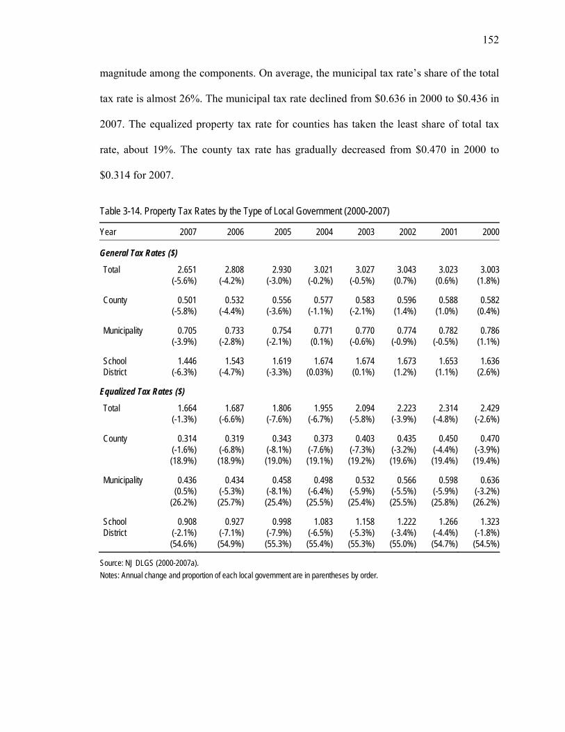
152
magnitude among the components. On average, the municipal tax rate’s share of the total
tax rate is almost 26%. The municipal tax rate declined from $0.636 in 2000 to $0.436 in
2007. The equalized property tax rate for counties has taken the least share of total tax
rate, about 19%. The county tax rate has gradually decreased from $0.470 in 2000 to
$0.314 for 2007.
Table 3-14. Property Tax Rates by the Type of Local Government (2000-2007)
Year 2007 2006 2005 2004 2003 2002 2001 2000
General Tax Rates ($)
Total 2.651 2.808 2.930 3.021 3.027 3.043 3.023 3.003 (-5.6%) (-4.2%) (-3.0%) (-0.2%) (-0.5%) (0.7%) (0.6%) (1.8%)
County 0.501 0.532 0.556 0.577 0.583 0.596 0.588 0.582 (-5.8%) (-4.4%) (-3.6%) (-1.1%) (-2.1%) (1.4%) (1.0%) (0.4%)
Municipality 0.705 0.733 0.754 0.771 0.770 0.774 0.782 0.786 (-3.9%) (-2.8%) (-2.1%) (0.1%) (-0.6%) (-0.9%) (-0.5%) (1.1%)
School 1.446 1.543 1.619 1.674 1.674 1.673 1.653 1.636 District (-6.3%) (-4.7%) (-3.3%) (0.03%) (0.1%) (1.2%) (1.1%) (2.6%)
Equalized Tax Rates ($)
Total 1.664 1.687 1.806 1.955 2.094 2.223 2.314 2.429 (-1.3%) (-6.6%) (-7.6%) (-6.7%) (-5.8%) (-3.9%) (-4.8%) (-2.6%)
County 0.314 0.319 0.343 0.373 0.403 0.435 0.450 0.470 (-1.6%) (-6.8%) (-8.1%) (-7.6%) (-7.3%) (-3.2%) (-4.4%) (-3.9%) (18.9%) (18.9%) (19.0%) (19.1%) (19.2%) (19.6%) (19.4%) (19.4%)
Municipality 0.436 0.434 0.458 0.498 0.532 0.566 0.598 0.636 (0.5%) (-5.3%) (-8.1%) (-6.4%) (-5.9%) (-5.5%) (-5.9%) (-3.2%) (26.2%) (25.7%) (25.4%) (25.5%) (25.4%) (25.5%) (25.8%) (26.2%)
School 0.908 0.927 0.998 1.083 1.158 1.222 1.266 1.323 District (-2.1%) (-7.1%) (-7.9%) (-6.5%) (-5.3%) (-3.4%) (-4.4%) (-1.8%)
(54.6%) (54.9%) (55.3%) (55.4%) (55.3%) (55.0%) (54.7%) (54.5%)
Source: NJ DLGS (2000-2007a). Notes: Annual change and proportion of each local government are in parentheses by order.

153
3-3-5. Property Tax Collection
The final step in the property tax administration process is the collection of
property taxes. After the property tax rate is determined by the county board of taxation,
the tax rate is reported to each municipality, which is responsible for collecting property
taxes. After collecting property taxes, the municipal government distributes the property
tax revenues to counties, school districts, and other special districts.
For the purpose of collecting property taxes and other revenues, a municipal tax
collector must be appointed by the governing body of each municipality for a four-year
term of office. The municipal tax collector must have the designation of certified tax
collector for a permanent appointment (Benecke, 2004a). The municipal tax collector is
prohibited by law from also serving as a member of the governing body and is subject to
control by the Division of Local Government Services (NJ OLS, 2005). The main
responsibilities of the municipal tax collector are to ascertain the amount of taxes due
from each taxpayer and inform each of them, to receive and account for tax payments, to
report periodically on the state of municipal finances, and to enforce timely payment of
taxes by the taxpayer (New Jersey Division of Taxation, 2001; Pareti, 2001).
Table 3-15 compares property tax collections by the type of local government,
indicating as well the annual percentage change and the share which each type of
government partakes of the total tax levies. The total property tax levy increased from
$14,195,070 in 2000 to $22,130,902 in 2007. During this period, counties, municipalities,
and school districts annually increased their property tax levies by 5.8%, 6.5%, and 6.5%,
respectively. In relative importance by type of local governments, 55 % of property tax
revenue is distributed to local school districts, 26% to municipalities, and 19% to county

154
governments, on average. The share of each government has been almost constant during
this period.
The statewide aggregate comparison of property tax collections by the type of
local government sheds light on the governments to be affected by changes in property
taxes involving limits on tax levies, or assessed valuation changes. Table 3-15 shows that
school districts would be affected most by such changes. Table 3-15 also provides the
cause of decreases in equalized property tax rates. During this period, while the equalized
tax rates has decreased (see Table 3-14), equalized property values (see Table 3-13) and
property tax levies (Table 3-15) have increased. This indicates that decreases in equalized
property tax rates are not caused by decreases in the amount of money financing local
public goods, but by increases in the property tax base, the property values.
Table 3-15. Property Tax Collections by the Type of Local Government (2000-2007)
Year 2007 2006 2005 2004 2003 2002 2001 2000
Total 22,130,902 20,914,762 19,567,777 18,377,494 17,253,985 16,035,254 14,991,991 14,195,070 (5.8%) (6.9%) (6.5%) (6.5%) (7.6%) (7.0%) (5.6%) (4.9%)
County 4,179,318 3,960,988 3,716,557 3,506,903 3,324,450 3,140,369 2,914,074 2,748,945 (5.5%) (6.6%) (6.0%) (5.5%) (5.9%) (7.8%) (6.0%) (3.4%)
(18.9%) (18.9%) (19.0%) (19.1%) (19.3%) (19.6%) (19.4%) (19.4%)
Municipality 5,882,848 5,459,896 5,038,923 4,686,968 4,387,009 4,079,641 3,876,752 3,713,573 (7.7%) (8.4%) (7.5%) (6.8%) (7.5%) (5.2%) (4.4%) (4.2%)
(26.6%) (26.1%) (25.8%) (25.5%) (25.4%) (25.4%) (25.9%) (26.2%)
School District 12,068,737 11,493,877 10,812,297 10,183,622 9,542,525 8,815,244 8,201,165 7,732,552 (5.0%) (6.3%) (6.2%) (6.7%) (8.3%) (7.5%) (6.1%) (5.7%)
(54.5%) (55.0%) (55.3%) (55.4%) (55.3%) (55.0%) (54.7%) (54.6%)
Source: NJ DLGS (2000-2007a). Notes: 1. Dollar amounts are in thousands. 2. Annual change and proportion of each local government are in parentheses by order.

155
3-4. Conclusion
In New Jersey, 21 counties, 566 municipalities, 616 school districts, and over 200
special districts are currently operating to provide public goods and services. Counties,
mainly as administrative arms of state government, are responsible for elections, the
judicial system, and county jails, among other services. While local school districts are
responsible for only primary and secondary education, municipalities are responsible for
a wide range of local public services such as police and fire protection, water, sewerage,
garbage collection, etc. In addition, special districts also deliver a broad range of public
services, including fire protection, water, sewerage, and garbage collection.
Local governments represent about 49% of total state-local expenditure in New
Jersey. Financial responsibility for providing most public services is commonly shared
between the state government and local governments. The review of government
expenditure reveals that there is a general correspondence between the real assignment of
service responsibilities and the theoretical suggestions for the assignment of functions
among levels of governments, including economies of scale, economies of scope,
proximity to beneficiaries, and so on.34
With a few exceptions, local governments are responsible for providing services
benefiting local residents such as fire and police protection, housing and community
development, sewerage, water, and waste management. These services are closely related
to property. On the other hand, state government is responsible for services requiring
large-scale infrastructure such as hospitals, highways, and public transit. In addition,
34. Stigler (1957), Musgrave (1959), Olson (1969), Oates (1972), Raimondo (1992), and Shah (1994), among
others, suggest guidelines for assigning responsibilities providing public services among different layers of governments.

156
broader-based services, such as public welfare, health, and income maintenance, are more
commonly the responsibility of state government.
To finance various services, local governments relied on their own source of
revenues for more than 68% of total local revenues, on average, during the period from
fiscal year 2003-04 through 2005-06. Own-source revenues essentially consist of
property taxes, user charges and fees, and other miscellaneous revenues. The remaining
32% of total local revenues comes from transfers from state government. Property tax is
the single largest source of revenue for counties, municipalities, and school districts,
accounting for more than half of total local revenues combined.
However, the relative importance of each source of revenue differs by the type of
local government. Although the reliance on the property tax differs by the type of local
government, all types of local government derive a considerable portion of their revenue
from the property tax. In addition, since 2000, the reliance on the property tax has
increased, regardless of the type of local government. On the other hand, the reliance on
state aid differs greatly by the type of local government. While school districts depend
heavily on state aid, the share of state aid in counties and municipalities is relatively
small. Municipalities also rely heavily on user charges and fees, although their share
declined during the period examined.
In New Jersey, the property tax is the local tax, as the property is assessed and tax
is collected at the municipal level for financing counties, municipalities, school districts,
and some special districts. The municipality functions as the tax collector for other local
governments. In New Jersey, the property tax is also considered both a residual tax and
an ad valorem tax. The residual tax means that the amount to be raised by the property

157
tax is the difference between the total budget and non-property tax revenues. The ad
valorem tax means that each taxpayer shares the tax burden according to the proportion
that his or her property bears to the total value of all property in the taxing district.
To ensure a fair property tax burden according to property value, the New Jersey
Constitution and state statues mandate that all property should be taxed in a uniform way,
at the same rate and assessment ratio within a taxing district, and that property should be
valued as its true value. To estimate the true value, which is defined as market value by
the state law, equalization, revaluation, and reassessment programs are performed in New
Jersey.
To relieve the burden of local taxpayers and to alleviate the reliance of local
government on the property tax, the state government imposes limits on increases in both
total property tax levies and tax rates. Despite such state-imposed limits, the share of
property tax in total local revenue has increased since year 2000. This is partly because
cuts in state aid and balanced budget requirements have collectively forced local
governments to become more self-reliant and thus to rely more on property taxes.
The examination of the property tax collections and the percentage which they
represent of total revenues by the type of local government illustrates the importance of
the property tax at the local level. The high burden on taxpayers, the local governments’
high reliance on the property tax, and the high visibility of the property tax intensify
taxpayers’ and local officers’ concerns with the property tax in the local budget decision.
The property tax is the most important revenue source which New Jersey local
governments can decide for themselves.
158
Chapter IV. Hypotheses, Research Models, and Data
This chapter derives hypotheses and develops empirical models examining the
hypotheses, based on the review of theoretical and empirical literatures on competition
among governments in Chapter II and on the understanding of the local government
structure and the practice of property tax administration in New Jersey reviewed in
Chapter III. Through the literature review in the Chapter II, it is concluded that there are
both theoretical and empirical reasons to believe that local governments engage in
competition regardless of what is the source of such competition and that, in general,
competition does affect fiscal behaviors of local governments. Chapter III shows that
New Jersey is a good empirical setting to test both inter- and intra-jurisdictional
competition with its highly fragmented local government structure, diversity in
institutions, and property tax base sharing among different types of local government.
In the first section, hypotheses, which are testable using data on local
governments in New Jersey, are developed from theoretical predictions of inter- and
intra-jurisdictional competition. Based on the theoretical models, the second section
defines four different public markets in which local governments are assumed to compete
with each other. The third section specifies two types of empirical models to test
hypotheses: a spatial policy interdependency model for the presence of inter- and intra-
jurisdictional competition; and panel or cross-sectional regression models for the effects
of inter- and intra-jurisdictional competition on government performance. In specifying
each empirical model, dependent and independent variables are identified and defined,
and their empirical measurements are provided. The final section presents the source of
data to be used for estimating the empirical models with descriptive statistics of variables.

159
4-1. Hypotheses
The primary purpose of this study is to investigate the presence of competition
among governments and the effect on government performance, which is addressed in the
remainder of this study. This section provides two sets of hypotheses drawn from
theoretical and empirical analyses on inter- and intra-jurisdictional competition. The first
set of hypotheses pertains to the presence of competition among governments and the
second set of hypotheses focuses on the consequences of competition in terms of
government performance. In addition, we develop hypotheses about the effect of local
government consolidation on government performance.
4-1-1. Existence of Inter- and Intra-jurisdictional Competition
We develop hypotheses about the presence of inter- and intra-jurisdictional
competition in property tax rate setting by New Jersey local governments. The New
Jersey property tax system and its local government structure have several unique
strengths for examining inter- and intra-jurisdictional competition. First, local
governments in New Jersey have considerable autonomy to pursue their own policies
although their purposes and scope of activities are controlled by the state legislature
through authorizing legislation. Local governments can initiate any policies that promote
the interests of their constituents and independently determine how they finance these
policies. The high level of autonomy of local governments raises the possibility that local
governments engage in competition.
Second, the property tax is the most important revenue source which New Jersey
local governments can decide upon themselves and the property tax base is shared by
160
municipalities, school districts, and counties. The co-occupancy of the property tax base
provides us the opportunity to examine simultaneously both inter- and intra-jurisdictional
competition. Third, because the property tax is the most visible among local fiscal
policies, citizens can easily monitor what happens to property tax rates but have a harder
time monitoring the quality of other fiscal policies. Therefore, it is highly likely that local
governments compete with each other through property tax rates.
A. Intra-jurisdictional Competition
Intra-jurisdictional competition theory suggests that co-occupancy of a tax base
between different levels of government or between co-equal taxing authorities generates
a negative externality. If one government raises its tax rate, this reduces the tax base and
thus the tax revenue of the other governments. Then, the other governments can respond
either by reducing their tax rates or by reducing expenditures. Thus, the sign of a reaction
by the other governments to a change in the tax rate of the government is ambiguous.
Although the sign of the reaction is theoretically ambiguous, a clear empirical prediction
of the theoretical analysis of intra-jurisdictional competition is the existence of
interdependence in setting tax rates by governments sharing the same tax base.
New Jersey is a convenient empirical setting to test the intra-jurisdictional
competition theory due to the property tax base sharing and to the coterminous
jurisdiction among local governments. In New Jersey, the property tax is the main
revenue source for local governments and the property tax base is co-occupied by
municipalities, school districts, and counties. In addition, New Jersey local governments
have the unique feature of coterminous jurisdiction. This means that although counties,
regional school districts, and consolidated school districts govern more than one

161
municipal jurisdiction, there are no partially overlapping boundaries among
municipalities, school districts, and counties.
The relationship among these three local governments in setting property tax rates
can be explained by the intra-jurisdictional competition theory. Although the
municipality and the school district may cooperate or coordinate in setting property tax
rates because of the low cost of cooperation or coordination, this also leads to
interdependence in tax rates. As theoretical analyses on intra-jurisdictional competition
suggest, it is likely that there is interdependence in setting property tax rates among
municipalities, school districts, and counties. This study examines the presence of intra-
jurisdictional tax competition in local property tax rate setting by testing the following
two hypotheses:
H1: School district property tax rates have an impact on municipal property tax rates. H2: County property tax rates have an impact on municipal property tax rates.
B. Inter-jurisdictional Competition
The underlying assumption of inter-jurisdictional competition theories is that
governments consider their neighbors’ tax rates when setting their own, and, therefore,
compete at some level with their competitors for economic and /or political reasons.
According to Tiebout, the tax competition theory, and the Leviathan hypothesis, the tax
rate of a jurisdiction influences the size of the tax base in neighboring jurisdictions and
consequently affects the budget constraints of other governments. As a result, a
jurisdiction’s tax rate indirectly affects the tax rates of neighboring jurisdictions, leading
to interdependence in local fiscal policies.

162
The above prediction is drawn from the pure competitive case where there are an
infinite or a large number of competitors. In strategic competition where there are a small
number of jurisdictions, the same empirical prediction of interdependence in tax rate
settings can be drawn. The strategic tax competition theory proposes that the tax rate in a
jurisdiction is directly influenced by the tax rates in neighboring jurisdictions because the
government in each jurisdiction considers the tax rates of other jurisdictions when setting
its own tax rate. This strategic behavior of each government leads to the interdependency
in tax rates among neighboring jurisdictions.
Yardstick competition theory also yields the same empirical prediction about
interdependence in tax rates among neighboring jurisdictions. In the yardstick
competition theory, it is assumed that citizen-voters use other governments’
performances as yardsticks to evaluate their incumbents’ performance and they decide
their votes based on this comparative performance evaluation. If citizen-voters take into
account tax rates in neighboring jurisdictions, incumbents are forced to consider tax rates
in neighboring jurisdictions too and, thus, set their tax rates in line with those in
neighboring jurisdictions due to a concern for reelection.
This study examines the above conclusion of interdependence in tax rates among
governments using municipal property tax rates. Inter-jurisdictional competition theories
do not provide the exact sign of the effect of competitors’ tax rates on a given
government’s tax rate. Therefore, the main idea underlying all theories on inter-
jurisdictional competition can be formalized and implemented empirically by examining
the following hypothesis:
H3: Property tax rate of a municipality is affected by property tax rates of competing jurisdictions.

163
4-1-2. Effect of Competition on Government Performance
To specify hypotheses about the effect of competition on government
performance, it is necessary to define government performance. The performance of local
governments can be evaluated using a wide variety of performance indicators such as
financial measures, efficiency measures, effectiveness measures, or responsiveness
indices (De Borger and Kerstens, 2000; Dollery, Wallis, and Worthington, 2001). Due to
the unavailability of reasonable data on inputs and outputs of local governments, most
empirical studies have focused on financial measures such as debt ratios, level of tax
rates, level of revenues, and level of expenditures.
Theoretical and empirical studies have explored the consequences of competition
among governments with respect to various government performance or behavior. The
conventional tax competition theory and the intra-jurisdictional competition theory have
focused on the allocative efficiency implications of competition while the Leviathan
hypothesis and the yardstick competition theory have investigated inter-jurisdictional
competition in terms of technical efficiency. In addition, all theories of inter- and intra-
jurisdictional competition have suggested the results of competition among governments
in terms of levels of tax rates, revenues, and expenditures.
We define local government performance in terms of property tax rates, allocative
efficiency, and technical efficiency. The property tax rate is selected because all theories
provide a theoretical prediction about the effect of competition on tax rates but this
prediction has been ignored in the empirical studies. The allocative efficiency and
technical efficiency measures are selected to evaluate which theoretical perspective is
correct among the competing inter-jurisdictional competition theories. While all theories

164
of inter-jurisdictional competition predict that competition leads to lower tax rates, they
have contrasting predictions about the effect of competition on government efficiency.
Thus, to examine which theory is correct, we have to use an efficiency measure of local
governments.
A. Effect of Inter-jurisdictional Competition
a. Effect on property tax rates
All theories of inter-jurisdictional competition have a common prediction that
inter-jurisdictional competition lowers the levels of tax rates, tax revenues, and
government expenditures. Oates (1972) suggests that local governments keep tax rates
low to attract a mobile tax base. This intuitive assertion has been examined by numerous
formal theoretical analyses, which is known as the conventional tax competition literature.
In particular, using a formal theoretical model, Hoyt (1991) demonstrates that
intensifying inter-jurisdictional competition by increasing the number of competing
governments lowers tax rates.
The Leviathan hypothesis posits also that the degree of inter-jurisdictional
competition is inversely related to the tax rate. In particular, Brennan and Buchanan
(1980) argue that fragmentation of governmental units enhances inter-jurisdictional
competition for mobile citizens or other mobile resources and this competition, in turn,
reduces governments’ taxing power. This prediction can be interpreted such that an
increase in the number of governments in a public sector or a public market leads to
lower tax rates. Formal theoretical analyses confirm the above intuitive assertions.

165
On the other hand, the yardstick competition literature is implicit regarding the
effect of inter-jurisdictional competition on the tax rate. The yardstick competition theory
suggests that citizen-voters’ retrospective voting strategy based on relative performance
evaluation induces local governments to engage in competition and to do better than
other jurisdictions. Based on this argument it can be predicted that yardstick competition
leads to lower tax rates if other things, especially expenditure levels, are equal. The
theoretical prediction about the effect of inter-jurisdictional competition on tax rates is
formalized into the following hypothesis, which is examined in terms of New Jersey
property tax rates.
H4. The degree of inter-jurisdictional competition is negatively related to the property tax rates.
b. Effect on allocative efficiency
Theories of inter-jurisdictional competition have contrasting views on the effects
of competition on allocative efficiency. While Tiebout, the Leviathan hypothesis, and the
yardstick competition theory predict that inter-jurisdictional competition leads to
allocative efficiency, the conventional tax competition theory predicts that inter-
jurisdictional competition results in allocative inefficiency. On the one hand, the
conventional tax competition theory suggests that local governments keep tax rates low to
attract mobile capital and this, in turn, leads to the under-provision of local public goods.
Hoyt (1991), among others, confirms this intuitive idea by demonstrating that an increase
in the number of jurisdictions in a public sector leads to a greater underprovision of
public goods and thus to allocative inefficiency.

166
On the other hand, Tiebout, the Leviathan hypothesis, and the yardstick
competition theory provide contrasting views on the allovative efficiency implication of
inter-jurisdictional competition. Tiebout states that the ability of individuals to “vote with
their feet” results in allocative efficiency in the provision of local public goods. The
Leviathan hypothesis and the yardstick competition theory suggest that inter-
jurisdictional competition can make self-interested politicians responsive and accountable
to the public interest. While the effect of inter-jurisdictional competition on allocative
efficiency was not examined in the formal theoretical analyses, the above argument
broadly suggests that inter-jurisdictional competition leads to allocative efficiency. We
address the question of which theoretical perspective is correct by testing the following
hypothesis:
H5: The degree of inter-jurisdictional competition has an impact on the allocative efficiency of local governments.
c. Effect on technical efficiency
While the Leviathan hypothesis and the yardstick competition theory have
focused on the technical efficiency implication of inter-jurisdictional competition, the
traditional tax competition theory has ignored it. The Leviathan hypothesis and the
yardstick competition theory argue that inter-jurisdictional competition fosters increased
efficiency in the production of local public goods. Formal theoretical analyses confirm
this intuitive idea by demonstrating that inter-jurisdictional competition leads to technical
efficiency by reducing government waste or rent. Tiebout also argues that citizen
mobility combined with competition among governments increases productivity and
reduces waste.

167
On the other hand, the conventional competition theory is silent about the
technical efficiency implication of inter-jurisdictional competition. The theoretical
analyses eliminate the technical efficiency issue by assuming that local governments are
benevolent welfare maximizers and that they use identical production techniques.
However, Oates (1972) provides a theoretical prediction about the effect of competition
on technical efficiency in terms of economies of scale. According to him, by reducing
jurisdiction sizes, increasing the number of local governments may result in the loss of
economies of scale and thus technical inefficiency. The contrasting two theoretical
perspectives on the technical efficiency implication of inter-jurisdictional competition are
investigated by testing the following hypothesis:
H6: The degree of inter-jurisdictional competition has an impact on the technical efficiency of local governments.
B. Effect of Public Market Share
Asymmetric tax competition models provide an empirical prediction about the
effect of jurisdictions’ relative population sizes on tax rates. In particular, Bucovetsky
(1991) and Wilson (1991) analyze the role of jurisdictions’ relative population sizes in
inter-jurisdictional competition. They predict that smaller or less populous jurisdictions
compete by setting tax rates lower than those of their larger competing jurisdictions.
Alternatively, relatively larger jurisdictions tend to have higher tax rates than smaller
competing jurisdictions because the supply of capital to the larger jurisdictions is less
responsive to their tax rate changes. To examine this prediction, this study tests the
following hypothesis:
H7: Communities’ relative population size to the total population of a public market is positively related to the property tax rate.

168
C. Effect of Local Government Consolidation
The consequences of local government consolidation can be explained by theories
of inter-jurisdictional competition and economies of scale. First, Oates’ (1972) economies
of scale thesis can be applied to explain the effect of government consolidation on
government performance. According to Oates, mergers of small units produce economies
of scale. If economies of scale are present in the provision of local public services, then
consolidation should be associated with lower tax rates and costs and greater productive
efficiency. Cost savings may result from the removal of administrative duplication, from
the lower input prices as a result of greater purchasing power, or from the use of
sophisticated technical equipment when the appropriate scale threshold is reached (Boyne,
1992).
The conventional tax competition theory argues that inter-jurisdictional
competition leads to sub-optimal levels of tax rates and, thus, to underprovision of local
public goods. The tax competition theory suggests reducing the degree of inter-
jurisdictional competition as the solution to the allovative inefficiency created by
competition for mobile factors. Thus, from the perspective of the tax competition theory,
the consolidation of small jurisdictions is expected to result in higher tax rates and to
enhance allocative efficiency by reducing the intensity of inter-jurisdictional competition.
Hoyt (1991) theoretically demonstrates that intensifying the degree of competition leads
to lower tax rates and to underprovision of local public goods.
On the other hand, if average cost curves are ‘U’ shaped, then very large
consolidated units may be subject to diseconomies of scale. In this case, higher costs may
arise because of the problems of delivering services to remote areas or because of

169
bureaucratic congestion (Boyne, 1992). In the beneficial view of inter-jurisdictional
competition, consolidation may also lead to technical inefficiency. As stated above,
consolidation reduces the intensity of inter-jurisdictional competition by reducing the
number of competing governmental units. Therefore, from the perspective of Tiebout, the
Leviathan hypothesis, and the yardstick competition theory, it is predicted that
government consolidation leads to higher tax rates and technical inefficiency.
The variation in types of New Jersey school districts provides us an opportunity to
examine the contrasting predictions about the effects of local government consolidation.
As we saw in Chapter III, New Jersey local school districts are classified into regular,
regional, and consolidated school districts. Consolidated school districts are formed
through the merger of two or more municipalities into a single school district. The
theoretical prediction on local government consolidation can be empirically examined by
comparing tax rates, allocative efficiency, and technical efficiency between communities
who are members of a consolidated school district and communities with regular school
districts.
H8: There is a systematic difference in tax rates between communities which are members of a consolidated school district and communities with regular school districts.
H9: There is a systematic difference in allocative efficiency between communities which are members of a consolidated school district and communities with regular school districts.
H10: There is a systematic difference in technical efficiency between communities which are members of a consolidated school district and communities with regular school districts.

170
D. Intra-jurisdictional Competition vs. Budget Referendum
The equilibrium analyses on intra-jurisdictional competition have examined the
allocative efficiency implication of intra-jurisdictional competition by comparing the
equilibrium tax levels of overlapping governments with those of unitary or coordinated
cases. The results of equilibrium analyses generally show that an increase in taxes by one
level of government results in a reduction in revenue to the other level of government.
This negative vertical externality causes one level of government to underestimate the
social marginal cost of raising tax revenue from the common tax base, since it ignores the
impact on others of choosing its tax rate. This, in turn, makes both levels of government
set a higher total tax rate on the shared tax base than they would if it was only taxed by
one level of government or a coordinated one. Consequently, the equilibrium analyses
conclude that intra-jurisdictional competition results in the super-optimal level of public
goods provision.
In New Jersey, the relationship between the Type I school district and the
municipality in fiscal policy decision making can be regarded as the coordinated case in
the theoretical analysis of the equilibrium tax levels. In a Type I school district, the
annual budget is prepared by the board of education whose members are appointed by the
mayor. The budget is submitted for approval to the board of school estimate which
consists of the mayor, two members of the school board, and two members of the
municipal governing body. On the other hand, the annual school budget must be
approved by citizen-voters in Type II school districts. The legal type of school districts,
therefore, reflects two different institutions: the budget referendum as a form of direct
democracy and intra-jurisdictional competition.
171
Direct democracy institutions have been touted as the means of controlling
politicians who tend to pursue their own interests in a representative democracy. The
central theoretical argument on direct democracy is that it provides citizens with a means
of selectively controlling their representatives on specific policies when such policies
deviate sufficiently far from citizens’ preferences (Freitag and Vatter, 2006). Several
studies have examined whether governments with the initiative or the referendum
demonstrate a stronger relationship between citizen preferences and policy output. In
general, the majority of the studies provide evidence for supporting the theoretical
prediction at the local and state level in Switzerland and the U.S, showing that direct
democracy institutions reduce government taxes, expenditures, and debt (for example,
Santerre, 1986; Matsusaka, 1995; Feld and Kirchgässner, 2001; Schaltegger and Küttel,
2002).
We can empirically examine the two theoretical predictions of intra-jurisdictional
competition by comparing tax rates and allocative efficiency between communities with
Type I school districts and communities the Type II school districts. However, the budget
referendum and intra-jurisdictional competition have contrasting effects both on tax rates
and on allocative efficiency. Considering these two contrasting effects, we draw the
following two conditional hypotheses:
H11: Property tax rates are lower in communities with Type II school districts if the budget referendum effect outweighs the intra-jurisdictional competition effect. On the other hand, property tax rates are higher in communities with Type II school districts if the intra-jurisdictional competition effect dominates the budget referendum effect.
H12: Allocative efficiency is higher in communities with Type II school districts if the budget referendum effect outweighs the intra-jurisdictional competition effect. On the other hand, allocative efficiency is lower in communities with Type II school districts if the intra-jurisdictional competition effect dominates the budget referendum effect.

172
4-2. Definition of Public Market
One main purpose of this study is to examine arguments about the presence and
the effects of competition from theoretical analyses of inter-jurisdictional competition. To
empirically test the presence and the effects of inter-jurisdictional competition, it is
required to assign neighbors or competitors to a given government by defining a public
market in which inter-jurisdictional competition is assumed to take place. However,
theories are silent about the proper definition of the public market and empirical studies
lack a consistent definition of the public market. We may draw quite different
conclusions on the existence and the effect of inter-jurisdictional competition by using
different definitions of the public market. Therefore, on the basis of theoretical arguments,
empirical feasibility, and empirical supports, this study defines the public market using
several criteria including contiguity, geographic distance, and county jurisdictional
boundaries.
4-2-1. Public Markets in Previous Empirical Studies
Theories on inter-jurisdictional competition are silent about how to properly
define a public market in which local governments are assumed to compete or interact
with each other. Therefore, it is clear that, in empirical studies, the choice of criteria for
defining the public market is somewhat arbitrary. Empirical studies on inter-jurisdictional
competition define the public market based on various criteria such as contiguity,
geographic distance, socio-economic similarity, or geo-political boundary. Reviewing the
definition of a public market in empirical studies reveals that there is a systematic

173
difference in defining the public market between studies on the presence of inter-
jurisdictional competition and those on the effect of it.
Most empirical studies on the effect of competition define public markets as fixed
geo-political boundaries such as counties (Eberts and Gronberg, 1988; Deller, 1990;
Hughes and Edwards, 2000; Bates and Santerre, 2006), SMSAs (Forbes and Zampelli,
1989; Schneider, 1989; Zax, 1989; Eberts and Gronberg, 1990; Grossman et al., 1999;
Bates and Santerre, 2006; Stansel, 2006), and states or provinces (Oates, 1985; Nelson,
1987; Hayes et al., 1998). One exception is Schneider (1989) who also defines the public
market based on contiguity. In these studies, all other governments within the same fixed
public market are assigned to a given government as its competitors. While some studies
(Nelson, 1987; Eberts and Gronberg, 1988 and 1990; Zax, 1989; Stansel, 2006)
distinguish between general-purpose and special-purpose governments, other studies
assume that all governmental units within a public market compete with each other,
regardless of the type and the level of government.
On the other hand, empirical studies on the existence of inter-jurisdictional
competition, which use spatial regression techniques, generally define the public market
as one which varies by government using geographic proximity criteria such as contiguity
or geographic distance. In these studies, a given government is assumed to compete with
other governments which share the same border with or locate within a certain distance
from the given government. Like empirical studies on the effect of inter-jurisdictional
competition, several studies define public markets as fixed geo-political boundaries such
as SMSAs (Ladd, 1992), statistical regions (Schaltegger and Küttel, 2002), and Cantons
(Brülhart and Jametti, 2006). In addition, some studies also use a fixed public market

174
which is defined by socio-economic similarity, regardless of geographic proximity (for
example, Schaltegger and Küttel, 2002; Hernández-Murillo, 2003; Solé-Ollé, 2003).
While the geographic area of a public market defined by geographic proximity
differs by community, the geo-political boundary-based public market is a fixed
geographic area. In addition, the geographic area of geo-political boundary-based public
market is much larger and, thus, the number of participants in the public market is larger
than that in the geographic proximity-based public market. This means that, while
empirical studies on the existence of competition have examined strategic competition
among a relatively small number of governments, the empirical literature on the effect of
competition, especially the Leviathan literature, has investigated the effect of relatively
pure competition among a large number of governments.
4-2-2. Four Different Definitions of Public Market
After reviewing theoretical models and empirical studies, and considering
empirical feasibility, this study defines the public market using four criteria: the first-
order contiguity, the second-order contiguity, the geographic distance, and the county
jurisdictional boundary. Based on the four different definitions of the public market, this
study calculates the average property tax rates of neighbors or competitors to test the
existence of inter-jurisdictional competition and measures the degree of inter-
jurisdictional competition to examine the effect of inter-jurisdictional competition on
government performance. In the following, how the public market is defined using the
four criteria is explained and theoretical rationales for each definition of the public
market are provided.

175
The simplest criterion to define the public market is the first-order contiguity.
Based on this criterion, municipalities are competitors of a given municipality if they
share a common border with the given municipality. The second-order contiguity assigns
municipalities sharing a common border with the first-order competitors to a given
municipality as its competitors. The second-order contiguity is cumulative and, thus,
includes all the first-order competitors as well. The geographic distance criterion defines
competitors based on the distance between centroids of municipalities. In a distance-
based public market, competitors are defined as municipalities located within a minimum
distance, which is required to assure that each municipality has at least one competitor.
The last criterion is the county boundary, which defines competitors of a municipality as
all other municipalities within the same county jurisdiction.
The definition of the public market should be driven by the theoretical models. In
mobility-based theories (Tiebout, tax competition, and Leviathan hypothesis), the
mobility of citizens, business firms, and other production factors is the central mechanism
which induces governments to compete with each other. On the other hand, the yardstick
competition theory suggests that competition derives from the comparative evaluation of
performance by citizen-voters. In this mechanism, information flow is crucial for citizen-
voters to evaluate their own government’s performance relative to that of other
governments. Therefore, the validity of criteria for defining the public market is
evaluated in terms of ease both of citizen mobility and of information flow.
The geographic proximity criteria, including contiguity and geographic distance,
have been used most frequently in the empirical studies on inter-jurisdictional
competition. Where mobility-based competition is concerned, geographic proximity

176
seems to be a reasonable a criterion to define the public market. When citizens are
dissatisfied with policies of their government, they may move to a more preferable local
government. Changing local government incurs emotional, social, informational, and
economic costs and these costs are proportional to the geographic distance (Eberts and
Gronberg, 1988; Schneider, 1989). Therefore, the mobility of residents which induces
local governments to engage in competition seems to occur among geographically close
jurisdictions. One other rationale for the use of geographic proximity is that adjacent
jurisdictions are more likely to experience similar economic shocks (Bordignon et al.,
2003) and, thus, information on policies of near-by jurisdictions may be a more
informative yardstick to citizen-voters (Vermeir and Heydels, 2006). In addition,
information about policies in nearby jurisdictions is more easily available to citizen-
voters because it is spread mainly through local and regional newspapers. Geographic
proximity, therefore, seems to be the appropriate criteria to account for both citizen
mobility and information flow.
The county has been treated as an appropriate geographic unit of the public
market because it is regarded as the political division that most reasonably approximates
the principal local labor and housing markets for residents within the county (Baird and
Landon, 1972; Zax, 1989).35 In New Jersey, it seems that the geographic boundary of a
county is large enough for residents to choose their residential location but small enough
to allow changes in local public services and property taxes without changes in
workplace location or social circles. In addition, on their websites, county governments
35. According to U.S. Census Bureau (2001), 43.4 million Americans changed their place of residence between
March 1999 and March 2000. While only 8.8 million (20.3%) of those who moved during that year moved to a different county within the same state and 8.4 million (19.4%) moved across state lines, 26.2 million (60.4%) chose to remain within the same county.

177
also provide property tax, public services, and other information on each municipality in
the county, which may be used by citizen-voters and municipal officials. Therefore, using
the county as a unit of public market is justified in terms of both resident mobility and
information flow.
In addition to the geographic proximity and geo-political boundary, it is also
reasonable to define the public market based on similarity in demographics or economic
conditions. In practice, several studies have defined the public market based on socio-
economic similarity in examining the presence of inter-jurisdictional competition.
However, this study does not use the socio-economic similarity-based public market
mainly due to the difficulty in empirically implementing the definition. Using statistical
methods such as Q-methods, cluster analysis, or factor analysis, it is possible to
categorize municipalities into a small number of groups which have similar socio-
economic conditions. However, this is very difficult when the number of observations is
substantially large. In addition, it is proved that in the empirical literature, geographic
proximity criteria performs better than socio-economic similarity criteria (Revelli, 2003).
4-2-3. Empirical Implementation
With a map of New Jersey, this study assigns competitors to each municipality
using the spatial econometric software, GeoDaTM. The distance-based public market is
defined by Euclidean distance between centeroids of municipalities in a polygon map and
the minimum Euclidean distance is 36,901.48. Table 4-1 provides descriptive statistics on
the number of competitors by public market. It shows that the number of competitors in
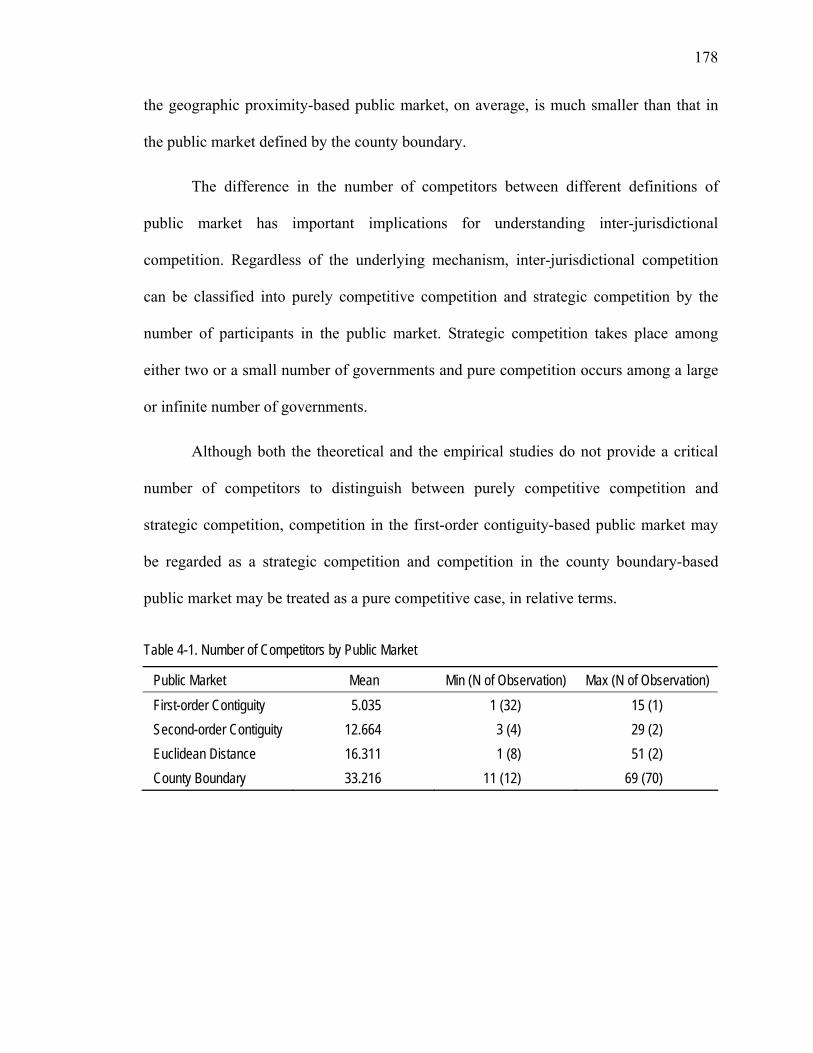
178
the geographic proximity-based public market, on average, is much smaller than that in
the public market defined by the county boundary.
The difference in the number of competitors between different definitions of
public market has important implications for understanding inter-jurisdictional
competition. Regardless of the underlying mechanism, inter-jurisdictional competition
can be classified into purely competitive competition and strategic competition by the
number of participants in the public market. Strategic competition takes place among
either two or a small number of governments and pure competition occurs among a large
or infinite number of governments.
Although both the theoretical and the empirical studies do not provide a critical
number of competitors to distinguish between purely competitive competition and
strategic competition, competition in the first-order contiguity-based public market may
be regarded as a strategic competition and competition in the county boundary-based
public market may be treated as a pure competitive case, in relative terms.
Table 4-1. Number of Competitors by Public Market
Public Market Mean Min (N of Observation) Max (N of Observation) First-order Contiguity 5.035 1 (32) 15 (1) Second-order Contiguity 12.664 3 (4) 29 (2) Euclidean Distance 16.311 1 (8) 51 (2) County Boundary 33.216 11 (12) 69 (70)

179
4-3. Research Models
The previous section developed hypotheses about the presence and the effect of
inter- and intra-jurisdictional competition. This section is devoted to specifing several
empirical models for examining the hypotheses, i.e., a spatial tax rate setting model for
the presence of competition, a combined municipal-school district tax rate model for the
effect of competition on property tax rates, a hedonic property value model for the effect
of competition on allocative efficiency, and a Tobit regression model for the effect of
competition on technical efficiency.
4-3-1. Existence of Competition
The spatial tax rate model is developed to simultaneously examine the presence of
intra-jurisdictional competition between municipalities and school districts (Hypothesis
1) and between municipalities and counties (Hypothesis 2) and inter-jurisdictional
competition among municipalities (Hypothesis 3) in setting property tax rates. For this
purpose, this study proceeds with two steps in developing the empirical analysis. First,
we develop a non-spatial municipal tax rate model, which includes only intra-
jurisdictional competition terms and control variables. Second, based on a spatial
autocorrelation test on OLS residuals of the non-spatial municipal tax rate model, we
identify and specify the proper spatial model between a spatial error model and a spatial
lag model. Following the model specification, we present the measurement of variables
and the empirical implementation strategy. Finally, we consider the econometric issues of
estimating the spatial tax rate models and provide solutions to these issues.

180
A. Municipal Property Tax Rate Model
We start with the non-spatial tax rate setting model relating municipal property
tax rates to school district property tax rates, county property tax rates, and other control
variables. Because theory provides no specific functional form, the natural starting point
is a linear additive specification. The non-spatial tax rate setting model can be expressed
as follows:
itMTR = 0 1 2it it it k itSTR CTR X uβ β β θ−+ + + + , (1)
where the subscripts i, t, and k represent the municipality (i = 1, …, 566), year (t = 2004),
and a time lag (k = 0, 1, or 4), respectively. MTRit, STRit, and CTRit are the property tax
rates of municipalities, school districts, and counties, respectively. Xit-k denotes a group of
exogenous control variables, and uit refers to an error term.
If the OLS residuals of the non-spatial tax rate setting model (Equation 1) exhibit
a significant spatial lag dependence or a spatial error dependence, the non-spatial tax rate
setting model would be mis-specified and, thus, should be specified either as a spatial lag
model or as a spatial error model (Anseline, 1988). The spatial lag tax rate setting model
and the spatial error tax rate setting model can be expressed as follows:
itMTR = 0 1 2 3it it ijt jt it k iti j
STR CTR w MTR Xβ β β β θ ε−≠
+ + + ∑ + + , (2)
itMTR = 0 1 2it it it k itSTR CTR X uβ β β θ−+ + + + , itu = ijt jti j
w uλ≠∑ + itε , (3)
where subscript j denotes the competitors of a given municipality i, ijt jti j
w MTR≠∑
represents a spatially lagged dependent variable, ijt jti j
w uλ≠∑ refers to a spatially lagged
error term, and itε is a well behaved error term.

181
The spatial lag model (Equation 2) and the spatial error model (Equation 3) seem
to be similar but, in fact, they have quite different predictions about the behavior of
governments in setting their tax rates.36 The spatial lag model posits that the tax rate of a
given municipality is influenced by the tax rates of competing municipalities and by other
determinants. The spatial lag model, therefore, is consistent with the arguments from
inter-jurisdictional competition theories. On the other hand, the spatial error model
implies that tax rate determinants omitted from the model are spatially correlated and this
leads to a spatial dependence in the dependent variable. Consequently, the spatial error
model suggests that there is no inter-municipal competition in setting tax rates.
What are the consequences of ignoring the spatial dependence in the dependent
variable or in the error term? Even when there is no spatial dependence in the dependent
variable, the estimation of the spatial lag model can lead us to conclude that there is
competition if the error term is spatially autocorrelated. In addition, ignoring the spatial
autocorrelation in the error term does not affect the unbiasedness of the estimated
parameters of β1, β2, and θ, but it reduces their efficiency (Hernández-Murillo, 2003). On
the other hand, ignoring the spatial dependence in the dependent variable causes a more
serious problem. When there is a spatial autocorrelation in the dependent variable,
omitting the spatially lagged dependent variable in estimating the model yields
inconsistent estimates of β1, β2, and θ (Brueckner, 2003). This suggests the importance of
careful examination of spatial autocorrelation in the dependent variable and in the error
term.
36. The spatial lag model has been used interchangeably with several different names such as spatial
autoregressive model and spatially lagged dependent model in the spatial econometric literature. We use the term, spatial lag model, throughout this study.

182
a. Municipal, school district, and county tax rates
To examine the presence of inter- and intra-jurisdictional competition in setting
property tax rates, this study estimates the non-spatial tax rate setting model (Equation 1)
and the spatial tax rate setting models (Equation 2 and 3), which link municipal property
tax rates to school districts’ and counties’ tax rates and/or to competing municipalities’
tax rates. As a result, the most important exploratory variables are the property tax rates
of school districts (STRit), counties (CTRit), and competing municipalities ( ijt jti j
w MTR≠∑ ).
The property tax rates are measured by the effective or equalized property tax rate and
stated dollars per $100 of assessed property value. The equalized property tax rate is
calculated as follows:
Equalized Property Tax Rate = Total Property Tax Levy $100Total Equalized Property Value
×
The effective property tax rate is calculated by dividing the property tax levy for
each type of local government by the total equalized property value in the municipality.
The property tax levy is the amount of money required to be raised through property
taxation. The property tax levy is determined by subtracting anticipated revenues from
other sources from the total appropriations in the budget. The equalized property value is
the market value, which is found through a massive statistical program by the Division of
Taxation. When comparing tax rates between communities or over a period of time, the
equalized tax rate is more useful than the general tax rate, which is used to calculate the
property tax bill.
183
b. Spatially lagged dependent variable
The spatially lagged dependent variable ( ijt jti j
w MTR≠∑ ) is the average municipal
property tax rate of competitors. While there is a unique match between a county and
municipalities within its jurisdiction and between a municipality and a school district
according to their respective geographic location, it is required to define a criterion in
order to assign a set of competitors to each municipality. In the second section of this
chapter, we define competitors based on four criteria: first-order contiguity, second-order
contiguity, Euclidean distance, and county jurisdictional boundary.
These four criteria are implemented by constructing a spatial weights matrix W =
{wijt, i,j = 1, …, 566, t = 2004}, where wijt is 1 for municipality j that is assigned as a
competitor to a municipality i according to the predefined four criteria and 0 otherwise.
The weights matrix W is row-standardized so that the sum of the weights equals unity for
each municipality i. Therefore, a spatially lagged dependent variable ( ijt jti j
w MTR≠∑ ) for
each municipality i is the simple average tax rate of competing municipalities, and a
spatially lagged error term ( ijt jti j
w uλ≠∑ ) for each municipality i is the average value of the
error term of its neighbors. In the tables of spatial regression outputs, the simple average
tax rate of competitors ( ijt jti j
w MTR≠∑ ) is denoted by WMTRit.
It can be argued that it is better to give different weights to competitors by
distance or by their socio-economic characteristics.37 However, we give equal weights to
all competitors of a given municipality and use the simple average tax rate of competing
37. For example, Brueckner and Saavedra (2001), Buettner (2003), and Luna (2004) give different weights to
competitors by population size, revenue or expenditure size, or income level.

184
municipalities, based on the following rationale. Theories on inter-jurisdictional
competition posit that politicians consider competitors’ tax rates when setting their own
tax rates and that citizen-voters use neighboring jurisdictions’ tax rates as a yardstick to
evaluate their government’s performance. In doing this, politicians and citizens are not
likely to give different weights on the tax rates of competitors by the socio-characteristics
of competing jurisdictions or distance. Rather, it is more feasible that politicians and
citizens simply either consider a competing jurisdiction’s tax rate or disregard it.
c. Determinants of municipal property tax rates
A local government’s fiscal decisions are influenced by its demographic and
economic environment, its fiscal capacity, and its political institutions. These factors are
grouped in the matrix Xit-k. The inclusion of various control variables serves to determine
the robust influence of the independent variables on the municipal property tax rates
(MTRit). These control variables are selected based on the theoretical and empirical
literature on the determinants of local fiscal policy. The shorthand name, the definition,
and the empirical measurement of control variables are as follows:
PMTLit-1 : Municipal property tax levy per capita = Total property tax levy for municipal purposes ($1,000)÷Estimated population;
PMSAit-1 : State aid to municipality per capita = Total state formula aid to municipality ($1,000)÷Estimated population;
POPit-1 : Municipal population = Estimated population as of July 1 (1,000 persons); POPSit-1 : Square of estimated population; POPDit-1 : Municipality population density = Estimated population (1,000 persons)÷ Land area
(square mile); INCit-1 : Personal income = Total personal income ($1,000)÷ Number of taxpayer plus
dependents; POVit-1 : Poverty rate = Number of children aged 5-17 receiving Temporary Assistance for
Needy Families (TANF)÷Estimated population (1,000 persons);

185
RBPit-1 : Residential building permits = Total number of new residential units authorized for construction;
UERit-1 : Unemployment rate = Estimated number of unemployment÷Estimated number of labor force×100;
P65it-4 : Percent of population aged 65 or over in 2000 = Number of population aged 65 or over ÷ 2000 census population×100;
PBAit-4 : Education level = Number of population over age 25 with a bachelor’s degree (BA) or higher in 2000÷ 2000 census population ×100;
PAAit-4 : Percent of African-American population in 2000 = Number of African-American÷ 2000 census population ×100;
PHOit-4 : Percent of home ownership in 2000 = Total number of owner-occupied units÷Total number of occupied units×100;
CRIit-4 : Crime rate = Total number of offenses reported in 2000÷ 2000 census population ×1,000;
DDit : Direct democracy institution = Dummy (1 if municipality has initiative and/or referendum and 0 otherwise);
CONSOLit : Member of a consolidated school district = Dummy (1 if a community is a member of a consolidated school district and 0 otherwise );
INTRAit : Relationship between municipalities and school districts = Dummy (1 if a school district is a Type II school district and 0 otherwise);
FMG1it : Elected governing body and chief executive form of municipal government = Dummy (1 if both governing body and chief executive are elected by voters and 0 otherwise); and
FMG2it : Elected governing body-administrator form of municipal government = Dummy (1 if a municipality operates under township, village, or commission form and 0 otherwise).
The property tax rates depend on the level of revenues necessary for financing
local public services. As shown in Chapter III, the property tax is levied to support the
residual costs of local governments after all other revenue sources have been anticipated.
To control for the amount of money to be raised through property taxes, we include
municipal property tax levy (PMTLit-1). We expect the property tax levy to have a
positive impact on municipal tax rates because a higher tax rate is needed to support
greater expenditures.

186
To control for other sources of revenue, we include state aid to municipalities per
capita (PMSAit-1). Intergovernmental transfers have been found to have an impact on the
fiscal behavior of recipient governments. The literature suggests that grants-in-aid
increase the spending of the recipient government (Gramlich, 1977; Inman, 1979; Dye,
1990) and reduce tax levels but not as much as in spending (Wildasin, 1986; Dye, 1990;
Raimondo, 1992; Fisher and Papake, 2000). State aid to municipalities allows
municipalities to reduce property tax rates and, thus, is expected to have a negative effect
on municipal tax rates.38
Population (POPit-1) and population density (POPDit-1) are included to capture the
potential economies of scale in providing local public services. The sign of the
coefficients of these variables is ambiguous since it depends on whether or not scale
economies exist in providing local public services. If scale economies are present,
population and population density are expected to have negative impacts on municipal
tax rates. We also include squared population (POPSit-1) to allow for a non-linear
relationship between population and municipal tax rates. The squared population can
have either a negative or a positive impact on municipal tax rates.
Population structure variables are included to capture their impacts on the demand
for local public services and, thus, on municipal tax rates. The population structure
38. Other revenue sources are certainly important in a municipality’s tax decisions. Other than the property tax
levy and the state aid, we consider per capita municipal expenditures and per capita miscellaneous revenues. We omitted expenditures and miscellaneous revenues due to severe multicollinearity. Pearson’s correlation coefficients show that these variables are highly correlated with property tax levies and with state aid. The correlation coefficients are as follows:
Tax Levy State Aid Expenditures State Aid 0.923 Expenditures 0.999 0.936 Miscellaneous Revenues 0.994 0.950 0.998 Notes: All Coefficients are significant at .01 significance level.

187
variables are the poverty rate (POVit-1), the percent of those aged 65 or more (P65it-4), the
percent of African-Americans in the population (PAAit-4), the percent of homeowners
(PHOit-4), the education level (PBAit-4), and the crime rate (CRIit-4). These variables also
represent the fiscal capacity or economic wealth of municipalities. The poverty rate, the
percentage of senior people, the percentage of African-Americans, and the crime rate are
expected to have positive effects on municipal tax rates because they present a high
demand for public services and weak fiscal capacities. The others can have either
negative or positive effects on municipal tax rates since they represent a high demand for
public services and strong fiscal capacities.
To control for the economic condition and the fiscal capacity of a municipality,
we include the unemployment rate (UERit-1), personal income (INCit-1), and residential
building permits (RBPit-1). Since total property value increases with new construction, the
residential building permit is expected to exert a negative effect on municipal tax rates.
Personal income and the unemployment rate may also reflect a high demand for
municipal services. The unemployment rate is expected to have a positive effect since it
represents a high demand for public services and weak fiscal capacity. Personal income
may have either a positive or a negative effect because it a reflects high demand for
public services and strong fiscal capacity.
A local government’s political institutions also influence its fiscal decisions. To
characterize the municipal political environment, we include a dummy variable for
municipalities with a direct democracy institution (DDit) and dummy variables for forms
of municipal government (FMG1it and FMG2it). To capture the differences in the
relationship between municipal governments and school districts, we also include a

188
dummy variable for municipalities which are a member of a consolidated school district
(CONSOLit) and a dummy variable for municipalities with a Type II school district
(INTRAit). We have no prior expectation on the sign of the coefficients associated with
these political institutional variables.
B. Hypothesis Test
a. Intra-jurisdictional competition
As we saw in the Chapter III, the main revenue source of local governments in
New Jersey is the property tax and the property tax base is shared among municipalities,
school districts, and counties. This tax base co-occupancy among three types of local
governments is exactly the case which is examined in intra-jurisdictional competition
theory. Thus, it is hypothisized that municipal property tax rates are affected by school
district tax rates (Hypothesis 1) and county tax rates (Hypothesis 2).
Since the direction of one government’s reaction to the changes in tax rate of the
other governments is theoretically ambiguous, Hypothesis 1 and Hypothesis 2 are tested
by examining the statistical significance of the coefficients on the school district tax rates
(β1) and the county tax rates (β2), respectively. In addition, the relationship between intra-
and inter-jurisdictional competition can be investigated by the changes in the statistical
significance and the magnitude of the coefficients on the school district tax rates (β1) and
the county tax rates (β2) between the non-spatial tax rate setting model (Equation 1) and
the spatial tax rate setting models (Equation 2).

189
b. Inter-jurisdictional competition
Although mobility-based theories (Tiebout, the tax competition theory, and the
Leviathan hypothesis) and the information-based yardstick competition theory provide
different mechanisms whereby local governments are induced to compete with each other,
they have in common a prediction that the tax rate of a jurisdiction is influenced by its
neighboring or competing jurisdictions’ tax rates. Based on the theoretical argument, we
set the Hypothesis 3 that the property tax rate of a municipality is affected by the property
tax rates of competing municipalities.
Testing Hypothesis 3 involves three steps in the spatial analysis: 1) Moran I tests
(Moran, 1950) on municipal property tax rates (MTRit), 2) Lagrange-Multiplier (LM) and
robust LM tests on OLS residuals of the non-spatial tax rate setting model (Equation 1),
and 3) a significance test on the coefficient of the spatially lagged dependent variable
(WMTRit) in the spatial lag tax rate setting model (Equation 2). In the first step, if the
Moran I test on municipal property tax rates shows no spatial autocorrelation, Hypothesis
3 is rejected. In the second step, if the LM and robust LM tests on the OLS residuals of
the non-spatial municipal tax rate model suggest that the spatial error model is the correct
model, then Hypothesis 3 is also rejected.
In the final step, Hypothesis 3 is tested by examining the statistical significance of
the coefficient on the spatially lagged dependent variable. Since the theory of inter-
jurisdictional competition shows that the slope of the reaction function can be either
positive or negative (Brueckner and Saavedra, 2001), the proper test for the presence of
inter-jurisdictional competition is a statistical significance test on the estimated spatial
slope coefficient (β3). Consequently, only if the Moran I tests on the dependent variable

190
and LM and robust LM tests on the OLS residuals of the non-spatial model support the
presence of spatial dependence in the dependent variable and the spatial slope coefficient
of the spatial lag model is statistically significant, we can provide the evidence supporting
the presence of inter-jurisdictional property tax competition.
C. Estimation Strategy and Econometric Issues
a. Estimation strategy
Before proceeding to the spatial regression analysis, this study examines if there
is a discernable spatial autocorrelation in municipal property tax rates (MTRit) and thus a
spatial framework is required to analyze the property tax rate setting. For this purpose, we
examine spatial dependence in municipal property tax rates using a quantile map. Then,
we perform a formal spatial autocorrelation test on the municipal property tax rates by the
Moran I statistic which calculates a linear association between the tax rate of a given
municipality and a weighted average of its competitors. Corresponding to the four
different public markets defined in the previous section, four different spatial weight
matrixes are used to compute the Moran I statistics.
Based on the results of the Moran I tests on the municipal property tax rates, we
decide whether or not to proceed to the spatial analysis. If the results show that there is no
spatial autocorrelation in municipal property tax rates, we reject Hypothesis 3 that there is
competition among municipalities in setting property tax rates. As a result, we stick to the
non-spatial regression analysis, which examines only intra-jurisdictional competition in
setting property tax rates. On the other hand, if we find a statistically significant spatial
autocorrelation in municipal property tax rates, we precede to the next step of the spatial
analysis.

191
To find out whether a spatial lag model or a spatial error model is more relevant
to analyze the property tax rate setting, we perform a spatial autocorrelation test on the
OLS residuals of the non-spatial tax rate setting model. Since the Moran I test is unable
to tell which of the two spatial models is the appropriate model (Brueckner, 1998), we
use LM and robust LM tests developed by Anselin et al. (1996) for spatial lag
dependence and spatial error dependence in the OLS residuals. In identifying the proper
spatial regression specification, we follow Anselin’s (2005) “spatial regression model
selection decision rule” (pp.198-200). The selected spatial lag or spatial error model is
estimated either by an Instruments Variable (IV) or by a Maximum Likelihood (ML).
b. Econometric issues and solutions
As discussed above, competing municipalities’ tax rates (WMTRit) affect a given
municipality’s tax rates (MTRit). At the same time, these competing municipalities’ tax
rates are influenced by the given municipality’s tax rates. If this underlying feature of the
model is correct, competing municipalities’ tax rates are endogenous. In addition, school
district tax rates (STRit) and county tax rates (CTRit) are also suspected to be endogenous.
It may not be realistic to assume that the county reacts to each of the municipalities’ tax
rates when setting property tax rates. However, even if the county tax rates were
exogenous, some correlation could remain between this variable and the error term, due
to the existence of common shocks to both tax rates. To solve the endogeneity issues
associated with the three mentioned variables, we estimate tax rate setting equations
using either IV or ML estimation.
Since school district tax rates and county tax rates are suspected to be endogenous,
we obtain OLS residuals for LM tests by estimating the non-spatial tax rate setting model
192
(Equation 1) by a two-step IV approach. In the first stage, the county property tax rate
and school district property tax rates are regressed on exogenous explanatory variables
(Xit-k) of Equation (1) and instrument variables. In the second stage, the fitted values of
county property tax rates (CTRit_HAT) and school district property tax rates (STRit_HAT)
are used in estimating the Equation (1) by OLS to obtain residuals used to test spatial
dependence by LM tests.
We also use a two-step IV approach to estimate the spatial lag model (Equation 2).
For this purpose, we first create spatially lagged exogenous explanatory variables (WXit-k)
and the spatially lagged dependent variable (WMTRit) by using GeoDaTM. In the second
stage, the spatially lagged explanatory variables, and county and school district
demographic variables are used as instruments for the endogenous spatially lagged
dependent variable, school district tax rates, and county tax rates. This two step IV
approach is performed by Stata’s IV generalized moments method (GMM) estimation
developed by Baum, Schaffer, and Stillman (2007).
On the other hand, for estimating the spatial error tax rate setting model
(Equation 3), we regress school district tax rates, and county tax rates on county
demographic variables, school district demographic variables, and all exogenous
explanatory variables of the non-spatial tax rate setting model (Equation 1). Then, the
fitted values of county property tax rates and school district property tax rates are used to
estimate the spatial error tax rate setting model (Equation 3) by using Kelejian and
Prucha’s (1999) GMM in the spdep package in R.

193
4-3-2. Effect of Competition on Property Tax Rates
We develop a combined property tax rate model to examine the effect of inter-
jurisdictional competition (Hypothesis 4), market share (Hypothesis 7), school district
consolidation (Hypothesis 8), and intra-jurisdictional competition (Hypothesis 11). All
theories of inter-jurisdictional competition have a common prediction that competition
leads to lower tax rates. On the other hand, intra-jurisdictional competition theory posits
that the combined tax rate of two overlapping government is higher than a coordinated or
unitary government’s tax rate. However, these theoretical predictions have not been
empirically examined, while empirical studies have exclusively focused on the effect of
competition on government size or on public sector size.
A. Combined Municipal-School District Tax Rate Model
In New Jersey, the relationship between a municipality and a Type I school
district can be regarded as a coordinated case compared to that between a municipality
and a Type II school district. The variation in the relationship between the municipal
government and the school district gives us a unique opportunity to investigate the effect
of intra-jurisdictional competition. To test the effect of inter- and intra-jurisdictional
competition simultaneously, we, therefore, use the combined tax rate of the municipality
and the school district as the dependent variable.
The combined municipal-school district tax rate model can be specified as
follows:
itMSTR = 0 4 5 6 7it it i it it k t itCOM MS CONSOL INTRA X Tβ β β β β θ δ ε−+ + + + + + + , (4)
where the subscripts i, t, and k represent the municipality (i = 1, …, 566), year (t = 2001,
…, 2004), and a time lag (k = 0, or 1), respectively. MSTRit represents the sum of

194
municipal and school district property tax rates, COMit denotes the degree of inter-
jurisdictional competition, MSit is market share, CONSOLi is a dummy variable for a
community which is a member of a consolidated school district, INTRAit is a dummy
variable for a community with a Type II school district, Xit-1 is a matrix of exogenous
control variables, Tt is a group of dummy variables for years with an exception of 2001,
and εit is well behaved error term.
a. Measures for the degree of inter-jurisdictional competition
One of the most important independent variables is the degree of inter-
jurisdictional competition. Following the previous empirical literature, this study uses
two kinds of measures for inter-jurisdictional competition: the number of municipal
governments in a public market (COMit) and a measure of public market share (MSit).
These two measures for the degree of inter-jurisdictional competition are also included as
independent variables in a hedonic property value model and a technical efficiency model
which are specified in the following two sub-sections.
Two alternative measures of inter-jurisdictional competition have been used in
examining the effect of competition on government performance: the number of
competing governments and the market share. Most empirical studies employ the number
of governmental units in a public market (Oates, 1985; Nelson, 1987; Zax, 1989; Stansel,
2006). Some employ a market-share measure analogous to concentration ratios used in
the private sector (Eberts and Gronberg, 1990). Others measure the inter-jurisdictional
competition using both kinds of measures. Either one alone cannot capture inter-
jurisdictional competition.

195
We measure the degree of inter-jurisdictional competition as the total number of
municipalities per 1000 persons in a public market, which is defined in the previous
section based on contiguity, distance, and the county boundary. To account for widely
varying sizes of public markets, the number of municipalities is divided by the population
of the public market. Since the number of local governments provides a measure of
alternative suppliers of local public services in a given public market, a greater number of
municipalities implies more intensive inter-jurisdictional competition.
Under this measurement of inter-jurisdictional competition, it is, however,
impossible to discriminate competition among municipalities from competition among
school districts. This is because, in New Jersey, jurisdictions of municipalities and school
districts are identical with the exception of 70 communities which are members of
consolidated school districts. As a result, the measure for the degree of inter-municipal
competition is almost identical to the measure for the intensity of inter-school district
competition. Nevertheless, the total number of municipalities and school districts in a
public market is not appropriate since a municipal government in one jurisdiction does
not compete with school districts in other jurisdictions and vice versa.
The second measure of inter-jurisdictional competition is a public market share,
analogous to concentration ratios used in the private sector. To measure the degree of
inter-jurisdictional competition, some studies borrow the Herfindhal-Hirshman index
(HHI) or the four-firm concentration ratio from the private sector. This kind of inter-
jurisdictional competition measure reflects the distribution of market share between
participants in a public market. However, due to the difficulty in implementing the HHI
or the four-firm concentration ratio, this study measures the public market structure by a

196
simple market share, which is calculated as MSit = Pim/Pm, where Pim is the population of
municipality i in public market m, and Pm is the respective public market’s population.
When the public market is defined based on contiguity and distance criteria, it is
very difficult to calculate the HHI because the public market varies by each jurisdiction.
No spatial econometric software provides a function to calculate such an index and
calculating the index manually is a very demanding job when the number of observations
is substantially large. In addition, when the public market is defined by contiguity and
geographic distance criteria, a concentration index, such as the four-firm concentration
ratio, cannot be used because some jurisdictions have fewer than four neighbors or
competitors.
The number of governmental units in a public market is a more direct measure for
inter-jurisdictional competition and better reflects theories of inter-jurisdictional
competition than the market concentration measure. Tiebout, the tax competition theory,
and the Leviathan hypothesis are based on the mobility of residents among competing
governmental units. The yardstick competition theory is based on information of
competing jurisdictions being used as a yardstick for evaluating government performance.
Therefore, unlike in the private sector, measures for market concentration may not be
appropriate measures for the degree of competition in the public market and the number
of alternative or competing governmental units is more important than the public market
structure.
b. Control variables
The matrix Xit-1 includes factors which are assumed to have impacts on the
combined municipal-school district tax rates. Due to the possible endogeneity problem or

197
the lack of recent data, some control variables are lagged one year and others are lagged
four years, with the exception of political institutional variables which are almost time-
constant. The shorthand name, the definition, and the empirical measure of the control
variables are as follows:
CTRit : Effective county property tax rate = Total property tax levy for county purposes ($) ÷Equalized valuation ($)×100;
Ln_PMTLit-1 : Log of municipal property tax levy per capita = Log [Total property tax levy for municipal purposes ($1,000)÷Estimated population] ;
Ln_PSTLit-1 : Log of school district property tax levy per capita = Log [Total property tax levy for school purposes ($1,000)÷Estimated population];
PMSAit-1 : State aid to municipality per capita = Total state aid to municipality ($1,000)÷Estimated population;
PSSAit-1 : State aid to school district per capita = Total state aid to school district ($1,000)÷Estimated population;
POPit-1 : Municipal population = Estimated population as of July 1 (1,000 persons); POPDit-1 : Municipality population density = Estimated population (1,000 persons)÷ Land area
(square mile); INCit-1 : Personal income = Total personal income ($1,000)÷Number of taxpayer plus
dependents; Ln_POVit-1 : Log of poverty rate = Log [Number of children aged 5-17 receiving
TANF÷Estimated population (1,000 persons)]; RBPit-1 : Residential building permits = Total number of new residential units authorized for
construction; UERit-1 : Unemployment rate = Estimated number of unemployment÷Estimated number of
labor force×100; PSDit-1 : Percent of enrolled pupils resident = Total number of enrolled pupils resident÷
Estimated population×100; P65i : Percent of population aged 65 or over in 2000 = Number of population aged 65 or
over ÷ 2000 census population×100; PBAi : Percent of population with BA or higher in 2000 = Number of population over age 25
with a bachelor’s degree or higher÷ 2000 census population×100; PAAi : Percent of African-American population in 2000 = Number of African-
American÷ 2000 census population×100; PHOi : Percent of home ownership in 2000 = Total number of owner-occupied units÷Total
number of occupied units×100; CRIi : Crime rate = Total number of offenses reported in 2000÷ 2000 census
population×1,000;

198
DDit : Direct democracy institution = Dummy (1 if a municipality has initiative and/or referendum and 0 otherwise);
FMG1it : Elected governing body and chief executive form of municipal government = Dummy (1 if both governing body and chief executive are elected by voters and 0 otherwise); and
FMG2it : Elected governing body-administrator form of municipal government = Dummy (1 if a municipality operates under township, village, or commission form and 0 otherwise).
We add the percentage of enrolled resident pupils (PSDit-1), state aid to school
district per capita (PSSAit-1), the log of school district property tax levy per capita
(Ln_PSTLit-1), and dummy variables for years (Tt) to the control variables of the spatial
tax rate setting model (Equation 2). In addition, county property tax rates (CTRit) is
included as a control variable.
The tax rate depends on the level of revenues needed to finance public services.
As in the spatial tax rate model (Equation 2), the property tax levy for education
(Ln_PSTLit-1) is included to control for the amount of money, which is used to finance
education services, to be raised through the property tax. The tax levy for education is
expected to have a positive effect on the combined municipal-school district since a
higher tax rate is needed to support greater expenditures for education.
Aside from the property tax, school districts rely heavily on state aid to finance
public education (see Table 3-12). As the literature on intergovernmental transfers
suggests, state aid is expected to induce school districts to reduce property taxes.
However, it is also possible that state aid has a positive effect on the tax rate. In New
Jersey, the state’s foundation aid formula gives more state aid to school districts (with a
lower property tax base. Consequently, the effect of state aid to school districts on the
combined tax rate can be either positive or negative.

199
The percentage of enrolled resident pupils (PSDit-1) is included as a proxy for both
the demand for public services and the fiscal capacity of a community. On the one hand,
a larger percentage of resident students may represent a higher demand for public
services, especially public education and, thus, lead to higher tax rates to finance the
higher public services. On the other hand, the greater percentage of resident students may
reflect the weak fiscal capacity of a community and, thus, result in higher tax rates.
Consequently, the percentage of enrolled resident pupils is expected to have a positive
effect on the combined municipal-school district tax rate.
We include the county property tax rate (CTRit) to control for the interdependence
in the tax rate setting between county government and other types of local governments
within its jurisdictional boundary. As the intra-jurisdictional competition theory predicts,
county tax rates can have either a positive or a negative effect on the combined
municipal-school district tax rate. We also include year dummy variables (Tt) to control
for shocks that are common to all communities but change across the time periods.
B. Hypothesis Test
a. Inter-jurisdictional competition
All theories of inter-jurisdictional competition agree that the degree of inter-
jurisdictional competition is inversely related to tax rates (Hypothesis 4). Although the
measure for the degree of inter-jurisdictional competition (COMit) reflects inter-
municipal and inter-school district competition, both inter-municipal and inter-school
district competition are expected to reduce municipal and school district tax rates,
respectively. Therefore, the degree of inter-jurisdictional competition is expected to have
a negative impact on the combined municipal-school district tax rate (MSTRit). The

200
negative and statistically significant coefficient on the degree of inter-jurisdictional
competition (β4) confirms Hypothesis 4.
b. Market share
Regarding the relative size of competing jurisdictions, Bucovetsky (1991) and
Wilson (1991) posit that small jurisdictions in terms of population may have competitive
advantages and that they set their tax rates lower than those of their larger competitors.
Based on the asymmetric tax competition theory, we hypothesized that communities’
relative population shares of the total population of a public market are positively related
to the property tax rate (Hypothesis 7). This hypothesis is tested by examining the effect
of the market share (MSit) on the combined municipal-school district tax rate. The
positive and statistically significant coefficient on the market share (β5) support
Hypothesis 7.
c. Local government consolidation
We predict that there is a difference in tax rates between communities which are
members of a consolidated school district and communities with the regular school
district (Hypothesis 8). The effect of school district consolidation is captured by the
dummy variable for communities which are members of a consolidated school district
(CONSOLi). This dummy variable reflects the average difference in tax rates between
communities with a regular school district and communities which are members of a
consolidated school district. The test of Hypothesis 8 is a simple significance test of the
coefficient (β6) associated with the dummy variable CONSOLi because the sign is
theoretically ambiguous. However, we can investigate which theoretical perspective is
correct by examining the sign of the coefficient (β6).

201
d. Intra-jurisdictional competition vs. budget referendum
The effect of intra-jurisdictional competition (Hypothesis 11) is tested by
examining the sign of the coefficient of the dummy variable for communities with a Type
II school district (INTRAit). As stated in the hypotheses section, however, the dummy
variable reflects two contrasting effects, the intra-jurisdictional competition effect and the
budget referendum effect. The coefficient of this dummy variable (β7), therefore, could
have either a positive or a negative effect on the combined tax rate. The positive
coefficient indicates the dominance of the budget referendum effect and the negative
effect means that the intra-jurisdictional competition effect outweighs the referendum
effect.
C. Econometric Issues and Solutions
Among the control variables, the county tax rate (CTRit) is suspected to be
endogenous because of the reciprocal effect among municipalities, school districts, and
counties in setting tax rates. It my be more realistic to believe that a county government
does not respond to changes in the tax rates of municipalities and school districts within
its boundary due mainly to its larger size. However, some correlation may still remain
between the county tax rate and the error term even though the county tax rate is
exogenous. This is because some economic conditions have an impact on county, school
district, and municipal tax rates. Therefore, the estimated coefficient of the county tax
rate may pick up some spurious correlation. We include a set of time dummies to control
for shocks to all municipalities, school districts, and counties. This approach has been
used in previous empirical investigations to solve the potential endogeneity (for example,
Boadway and Hayashi, 2000; Esteller-Moré and Solé-Ollé, 2001).

202
4-3-3. Allocative Efficiency Model
The allocative efficiency model is developed to test the effect of inter-
jurisdictional competition (Hypothesis 5) and the effect of school district consolidation
(Hypothesis 9) on government allocative efficiency. There are two contrasting views on
the consequences of inter-jurisdictional competition and local government consolidation
in terms of government allocative efficiency. We can tell which theoretical perspective is
correct by testing the above two hypotheses.
A. Brueckner’s Property Value Maximization Thesis
Building on the conclusion that property value-maximizing behavior by local
officials can lead to a Pareto-efficient provision of local public goods (Brueckner, 1979),
Brueckner (1979, 1982) developed a theoretical model of property value determination
which can be used to test for allocative efficiency in local governments. In his model,
aggregate property value in a community which levies a property tax is an inverted U-
shaped function of its public good outputs, with the maximum occurring at the output
level which satisfies the Samuelson condition for Pareto-efficiency. Brueckner (1979,
1982) demonstrated that if a marginal increase in public spending has no effect on
aggregate property value in an open community, holding the housing stock fixed, then the
Samuelson condition for allocative efficiency in the provision of public goods is satisfied.
Brueckner (1979, 1982) empirically demonstrated that hedonic estimates of
property values can be used to test for allocative efficiency in local governments. By
estimating a hedonic regression model where the dependent variable is total property
value and the public good expenditure level is included as an independent variable, the

203
location of the data points on the hyper surface can be determined (Deller and Chicoine,
1993). A positive coefficient on expenditure would be interpreted as evidence against
systematic overprovision, while a negative coefficient means that the public good is not
being systematically underprovided. The same line of reasoning suggests that a zero
coefficient is evidence against both systematic underprovision and overprovision
(Brueckner, 1982; Brueckner and Wingler 1984).
Brueckner’s (1979, 1982) intriguing proposition has spawned numerous empirical
studies that test for allocative efficiency in government decision making. A cross-
sectional regression model relating property values to public expenditures and other
determinants of property values forms the basis for the efficiency test. Deller (1990),
Shah (1992), Deller and Chicoine (1993), and Taylor (1995), among others, use
Brueckner’s (1979, 1982) approach to test for allocative efficiency in the provision of
local public goods. Grossman, Mavros, and Wassmer (1999), Hughes and Edwards
(2000), and Bates and Santerre (2006) use Brueckner’s (1979, 1982) approach to examine
the effect of competition on allocative efficiency.
B. Hedonic Property Value Model
To investigate the effect of inter-jurisdictional competition, local government
consolidation, and local public market share, this study develops a property value model
based on the Brueckner’s (1979, 1982) theoretical model and empirical studies
employing his model. Because most empirical studies, such as, Deller (1990), Taylor
(1995), and Bates and Santerre (2006), employ a log-log specification, this study
specifies the hedonic property value regression model in a log-linear functional form. The
log-linear hedonic property value model is as follows:

204
_ itLn TPV = 0 8 9 10_ it it it it k itLn COM CONSOL INTRA Xβ β β β θ ε−+ + + + + , (5)
where subscripts i, t, and k denote the municipality (i = 1, …, 566), year (t = 2004), and a
time lag (k = 0, 1, or 4), respectively. Ln_ represents the natural logarithm, 39 TPVit
denotes total property values, COMit represents the degree of inter-jurisdictional
competition, CONSOLit is a dummy variable for communities which are members of a
consolidated school district, Xit-k refers to a matrix of exogenous control variables, and εit
is a well behaved error term.
a. Total property value
The dependent variable, total property value ($1,000), is measured by the total
equalized value of property subject to local property taxation for 2004. The total
equalized property value is calculated as follows:
Total Equalized Property Value = $Total Taxable Value of Land and Improvements 1000 State Equalization Ratio
÷
The land and improvements include vacant land, farm land, residential property, farm
homestead property, commercial property, industrial property, and apartments.
Machinery implements and telephone messenger system equipment are also subjected to
the property tax but are excluded from the total taxable property value. Data on the total
taxable value of land and improvements and the state equalization ratio come from the
Tax Table and the Abstract of Ratables provided by NJ DLGS, respectively.
b. Control variables
Based on Brueckner’s (1979, 1982) theoretical model and subsequent empirical
studies, the list of control variables for the hedonic property value model (Equation 5) 39. In some variables, the minimum value is zero. To take logarithms, we add to such values a unit of
measurement associated with that variable so as to assure the minimum value is greater than zero.

205
includes determinants of property value, demand factors for local public goods, and
political imitations. Expenditure variables are lagged one year since there is an inherent
time delay in public expenditures being capitalized into the value of property. All other
control variables are also lagged one or more years due to potential endogeneity and the
lack of available recent data. The shorthand name, the definition, and the empirical
measurement of control variables are as follows:
Ln_MSit : Log of market share = Log [Population of a municipality÷Total population of its respective public market];
Ln_TMBit-1 : Log of municipal budget = Log [Total expenditure on municipal purposes ($1,000)]; Ln_TSBit-1 : Log of school district budget = Log [Total expenditure on education ($1,000)]; Ln_MSSAit-1 : Log of state aid to the municipality and the school district = Log [Sum of state aid to
the municipality and the school district ($1,000)]; Ln_HOSit : Log of housing stocks = Log [Number of residential parcels]; LN_PCIVit : Log of percent of commercial and industrial property value = Log [Sum of commercial
and industrial property value ($1,000)÷Total property value ($1,000)×100]; Ln_MNRit-4 : Log of median number of rooms; Ln_HB70it-4 : Log of percent of housing built before 1970 = Log [Number of housing units built
before 1970÷Total housing units×100]; POPGit-1 : Population growth rate = Estimated population in year t - Estimated population in
year t-1÷Estimated population in year t-1×100; Ln_POPDit-1 : Log of municipality population density = Log [Estimated population (1,000
persons)÷ Land area (square mile)]; Ln_INCit-1 : Log of personal income = Log [Total personal income ($1,000)÷ Number of
taxpayer plus dependents]; Ln_POVit-1 : Log of poverty rate = Log [Number of children aged 5-17 receiving TANF÷Estimated
population (1,000 persons)]; Ln_RBPit-1 : Log of residential building permits = Log [Total number of new residential units
authorized for construction]; Ln_UERit-1 : Log of unemployment rate = Log [Estimated number of unemployment÷Estimated
number of labor force×100]; Ln_CRIit-4 : Log of crime rate = Log [Total number of offenses reported in 2000÷ 2000 census
population ×1,000]; DDit : Direct democracy institution = Dummy (1 if a municipality has initiative and/or
referendum and 0 otherwise);

206
INTRAit : Intra-jurisdictional competition between municipalities and school districts = Dummy (1 if a school district is a Type I school district and 0 otherwise);
FMG1it : Elected governing body and chief executive form of municipal government = Dummy (1 if both governing body and chief executive are elected by voters and 0 otherwise); and
FMG2it : Elected governing body-administrator form of municipal government = Dummy (1 if a municipality operates under township, village, or commission form and 0 otherwise).
Two government expenditures are included in the hedonic regression model: total
municipal expenditure (Ln_TMBit-1) and total school district expenditure (Ln_TSBit-1).
These two variables are used to test whether or not local public goods are provided in an
allocatively efficient manner by examining the significance and sign of their coefficients.
The coefficients on these variables can be positive, negative, or zero (see Brueckner,
1979, 1982). State aid to municipality and school district (Ln_MSSAit-1) is also deemed to
be important because of the relatively large percentage of total local revenues coming
from state sources (see Table 3-12). State aid is expected to have a positive effect on the
property value.
The hedonic property value model does not include tax variables as explanatory
variables. This is because the inclusion of tax variables as well as expenditure variables
in the property value equation violates local government budget constraints (Deller, 1990,
Shah, 1992). Therefore, the coefficient of local government expenditures shows how
property values change if local government expenditures are increased and taxes are
raised to cover the cost of that increase (Deller, 1990).
Several variables are used to capture the effect of housing stock characteristics on
the total property values. The total number of residential parcels (LN_HOSit) represents
the absolute size of a community’s housing stock and is expected to have a positive

207
impact on the property value. The median number of rooms (Ln_MNRit-4) and the
percentage of houses built before 1970 (Ln_HB70it-4) measure the quality of housing
stock. The former is expected to have a positive effect and the latter is expected to have a
negative impact on the property value. The percentage of commercial and industrial
property values (LN_PCIVit) is included to account for alternative land uses and there is
no a priori expectation on the sign of its coefficient.
To control for the effect of socio-economic characteristics of a community on
property values, the hedonic property value model includes population growth (POPGit-1),
population density (Ln_POPDit-1), personal income (Ln_INCit-1), poverty rate
(Ln_POVit-1), residential building permits (Ln_RBPit-1), unemployment rate (Ln_UERit-1),
and crime rate (Ln_CRIit-4). Population growth, population density, poverty rate,
unemployment rate, and crime rate are undesirable conditions and thus are expected to
have negative effects on property value. Personal income and residential building permits
are expected to be positively related to property value.
To control for the possible effect of political institutions on property value, the
hedonic model includes the direct democracy institution of municipality (DDit), a dummy
variable for a community with a Type II school district (INTRAit), and dummy variables
for the forms of municipal government (FMG1it and FMG2it). Finally, the hedonic model
also includes the public market share (Ln_MSit) to control for the relative population size
of a community to its respective public market’s population. We have no prior
expectation on the sign of coefficients on these variables.

208
C. Hypothesis Test
a. Inter-jurisdictional competition
In the previous section, we drew a hypothesis that inter-jurisdictional competition
affects allocative efficiency without specifying the exact direction of the effect
(Hypothesis 5). This is because various theories have contrasting views on the
consequences of inter-jurisdictional competition in terms of allocative efficiency. While
the tax competition literature suggests that inter-jurisdictional competition results in
inefficient resource allocation, Tiebout, the Leviathan hypothesis, and the yardstick
competition theory argue that it enhances allocative efficiency. The test of Hypothesis 5
is the simple significance test of the coefficient (β8) on the degree of competition (COMit).
By measuring the impact of the degree of inter-jurisdictional competition on
property value, this study may provide evidence to help discriminate between two
competing views on the effect of competition on government allocative efficiency:
Tiebout, the Leviathan hypothesis, and yardstick competition vs. the conventional tax
competition theory. A positive coefficient on the degree of inter-jurisdictional
competition implies that a greater number of governmental units are superior from a
property value perspective and thus confirms the beneficial views of inter-jurisdictional
competition.
b. Local government consolidation
The effect of school district consolidation on allovative efficiency (Hypothesis
10) is tested by the coefficient (β9) associated with the dummy variable for communities
which are members of a consolidated school district (CONSOLit). The dummy variable

209
captures the average difference in property values between communities which are
members of a consolidated school district and communities with regular school districts,
other things being equal. The test of Hypothesis 10 is a simple significance test because
we did not specify the sign of the effect the school district consolidation would have on
allocative efficiency due to the two contrasting theoretical predictions. By examining the
sign of coefficient, we may tell which theoretical prediction is correct between the two
competing perspectives: Tiebout, the Leviathan hypothesis, and yardstick competition v.s.
the conventional tax competition theory.
c. Intra-jurisdictional competition vs. budget referendum
The effect of difference in relationships between municipal government and
school district (Hypothesis 12) is captured by the dummy variable for communities with
the Type II school district (INTRAit). This dummy variable reflects both the efficiency
worsening effect of intra-jurisdictional competition and the efficiency enhancing effect of
the school budget referendum. Hypothesis 12 is tested by examining the statistical
significance and the sign of coefficient (β10) on the INTRAit. A positive coefficient
implies the dominance of the budget referendum effect and a negative coefficient
indicates the dominance of intra-jurisdictional competition.
4-3-4. Technical Efficiency Model
The technical efficiency model is constructed to test the effect of inter-
jurisdictional competition (Hypothesis 6) and the effect of school district consolidation
(Hypothesis 10) on government technical efficiency. To test Hypotheses 6 and 10, this
study uses a two-step procedure. In the first stage, the Data Envelopment Analysis (DEA)

210
efficiency model is used to measure technical efficiency scores for 566 New Jersey local
governments from 2001 to 2004. In the second sage, a Tobit censored regression model is
specified, taking into account the distributional characteristics of the technical efficiency
scores.
A. DEA Efficiency Analysis
Technical efficiency refers to the ability of an organization to avoid waste by
producing the maximum possible outputs from a given set of inputs or by achieving a
given level of outputs with the minimum inputs (Dollery, Wallis, and Worthington, 2001).
Various approaches have been applied to measuring technical efficiency. These
techniques can be classified into two major subgroups: 1) parametric methods, such as
Stochastic Frontier Analysis (SFA), Deterministic Frontier Analysis (DFA), and
Corrected Ordinary Least Squares (COLS), and 2) non-parametric methods such as Total
Factor Productivity (TFP), Free Disposal Hull (FDH), and the DEA (De Boger and
Kerstens, 1996a; Dollery, Wallis, and Worthington, 2001).40 For two reasons, this study
uses the DEA approach to measure the technical efficiency of New Jersey local
governments. First, the DEA approach allows for the decomposition of total technical
efficiency into pure technical efficiency and scale efficiency. Second, the DEA does not
require identifying a functional form or making distributional assumptions.
Based on Farrell’s (1957) frontier analysis, DEA approach is developed by
Charnes, Cooper, and Rhodes (1978) and Banker, Charnes, and Cooper (1984) among
others (De Borger and Kerstens, 1996a). DEA is a non-parametric mathematical 40. See De Boger and Kerstens (1996a) and Dollery, Wallis, and Worthington (2001) for a good review of
various techniques for measuring government efficiency and a good survey of empirical studies employing those techniques. See Charnes, Cooper, Lewin, and Seiford (1995) and Thanassoulis (2001) for a good description of the DEA.
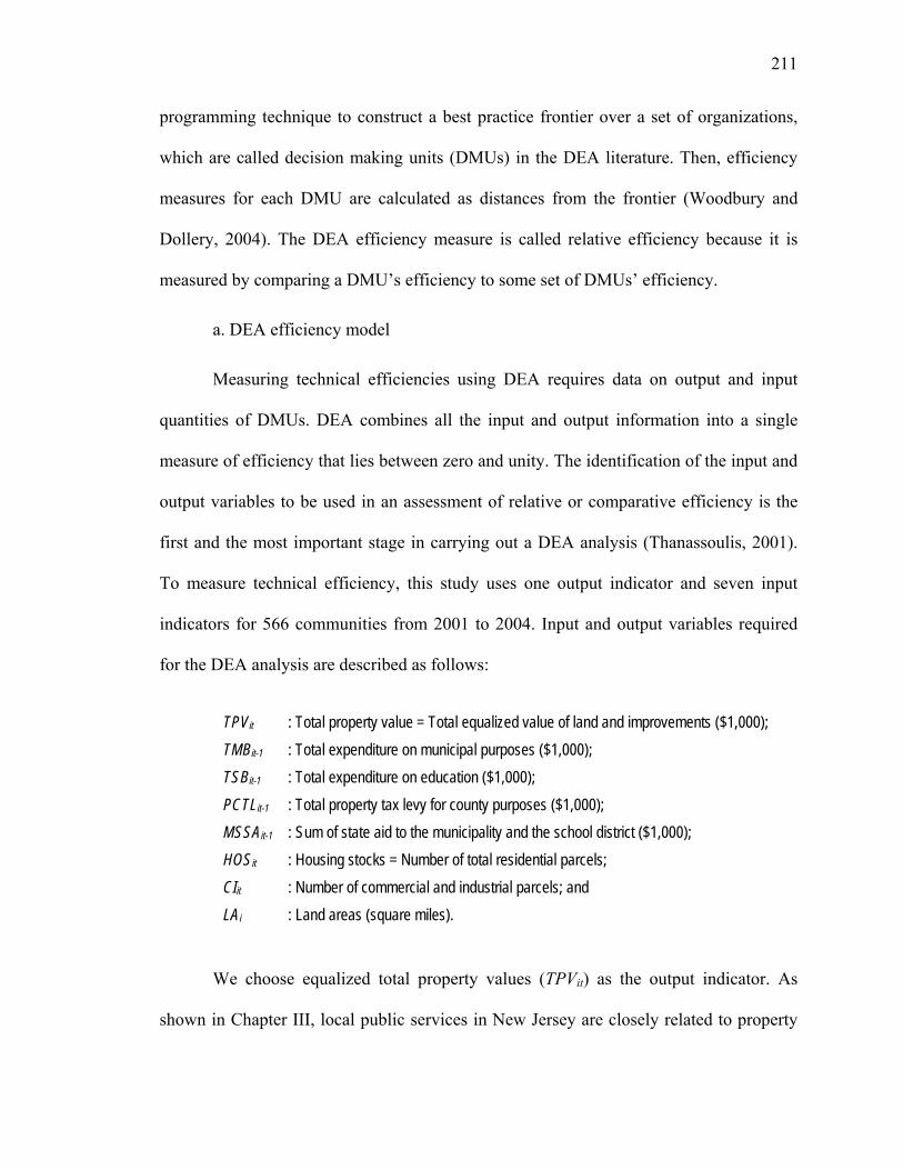
211
programming technique to construct a best practice frontier over a set of organizations,
which are called decision making units (DMUs) in the DEA literature. Then, efficiency
measures for each DMU are calculated as distances from the frontier (Woodbury and
Dollery, 2004). The DEA efficiency measure is called relative efficiency because it is
measured by comparing a DMU’s efficiency to some set of DMUs’ efficiency.
a. DEA efficiency model
Measuring technical efficiencies using DEA requires data on output and input
quantities of DMUs. DEA combines all the input and output information into a single
measure of efficiency that lies between zero and unity. The identification of the input and
output variables to be used in an assessment of relative or comparative efficiency is the
first and the most important stage in carrying out a DEA analysis (Thanassoulis, 2001).
To measure technical efficiency, this study uses one output indicator and seven input
indicators for 566 communities from 2001 to 2004. Input and output variables required
for the DEA analysis are described as follows:
TPVit : Total property value = Total equalized value of land and improvements ($1,000); TMBit-1 : Total expenditure on municipal purposes ($1,000); TSBit-1 : Total expenditure on education ($1,000); PCTLit-1 : Total property tax levy for county purposes ($1,000); MSSAit-1 : Sum of state aid to the municipality and the school district ($1,000); HOSit : Housing stocks = Number of total residential parcels; CIit : Number of commercial and industrial parcels; and LAi : Land areas (square miles).
We choose equalized total property values (TPVit) as the output indicator. As
shown in Chapter III, local public services in New Jersey are closely related to property

212
value. In addition, the capitalization literature has demonstrated that local government
policies are capitalized into property values. It is highly likely that the property values
capture important aspects of most public services provided by local governments. In
addition, property is the base of the local property tax, which is the main revenue source
for local governments in New Jersey. Therefore, the property values represent the ability
of local governments to generate revenues. With a strong property tax base, a community
can choose a high level of public services at moderate tax rates or a low level of services
at even lower tax rates. Consequently, local governments want to maximize their property
values. Based on Brueckner’s (1979, 1982) and his followers’ models and empirical studies
employing DEA, determinants of property values and local government expenditures are
used as input indicators. The expenditure variables are one year lagged, assuming that there
is a time delay in expenditure being capitalized into property values.
b. Orientation system and returns to scale
In calculating technical efficiency scores using DEA, we must specify two
characteristics of the DEA model: the orientation system and the returns to scale. The
DEA efficiency measure is based on estimates of the degree to which a DMU could have
secured more outputs for its input levels, or the degree to which it could have used fewer
inputs for its output levels (Thanassoulis, 2001). Therefore, we need to decide whether
the DMUs have more discretion over input or over output levels. According to
Thanassoulis (2001), the output orientation efficiency is appropriate when outputs are
controllable and the input orientation is appropriate when inputs are controllable. We
select the input orientation system, assuming that local governments take the output, the

213
property values, as exogenous and have substantial control over input variables,
especially expenditures.
The DEA approach constructs the non-parametric frontier as the piecewise linear
combination of all efficient DMUs in a sample (De Borger and Kerstens, 1996a). This
DEA frontier can be estimated either under constant returns to scale (CRS) or under
variable returns to scale (VRS). To construct the non-parametric frontier, while the CRS
approach compares all DMUs in a sample regardless of their size, the VRS approach
compares DMUs within a similar scale (Wetzel, 2006). Consequently, the CRS approach
produces an overall technical efficiency score which is a combination of pure technical
and scale efficiency and the VRS approach only calculates pure technical efficiency
(Hughes and Edwards, 2000).41 According to Worthington (2000), the CRS approach is
only appropriate where all DMUs are operating at an optimal scale. This study follows
the VRS approach, recognizing that local governments are not operating at an optimal
scale and pure technical efficiency is appropriate to examine the arguments from theories
of inter-jurisdictional competition.
B. Tobit Censored Regression Analysis
In the second stage, a technical efficiency regression model is developed to test
Hypothesis 6 and Hypothesis 10. As a result of the DEA analysis in the first stage, pure
technical efficiency scores for each community in each year are obtained. The technical
efficiency scores are used as the dependent variable in the technical efficiency regression
model. The selection of a regression model explaining differences in the technical
41. The difference between the VRS efficiency score and the CRS efficiency score indicates the presence of
scale efficiency. The scale efficiency score can be calculated from the difference between the VRS efficiency score and the CRS efficiency score.

214
efficiency scores among communities should consider the distributional characteristics of
the efficiency scores. As the technical efficiency scores are bounded below by unity, a
Tobit censored regression model is used.
a. Tobit censored regression model
The Tobit censored regression model is defined in terms of a latent variable (De
Borger and Kerstens, 1996b). The latent technical efficiency ( *itTE ) is not directly
observable. Instead, we can observe a technical efficiency score (TEit) which is censored
at the limit level of unity, thus partly masking the true value of *itTE . The TEit is observed
when *itTE is less than unity, while the TEit equals unity when *
itTE equals or is greater
than unity. Therefore, the Tobit technical efficiency model can be specified as follows:
*itTE = 0 11 12it i it k t itCOM CONSOL X Tβ β β θ δ ε−+ + + + + , (6)
**
*
111
ititit
it
TETE ifTE
TEif⎧ <
= ⎨≥⎩
where the subscripts i, t, and k represent the community (i = 1, …, 566), year (t = 2001,
…, 2004), and a time lag (k = 0 or 1), respectively. TEit is the DEA technical efficiency
score, COMit is the degree of inter-jurisdictional competition, CONSOLit is a dummy
variable for a community which is a member of a consolidated school district, Xit-1 is a
matrix of exogenous control variables, Tt is a group of dummy variables for each year
with an exception of 2001, and εit is a error term.
b. Independent variables and hypothesis test
The degree of inter-jurisdictional competition (COMit) and the dummy variable
for communities which are members of a consolidated school district (CONSOLit) are two

215
independent variables. Hypothesis 6 and Hypothesis 10 are tested by examining the
significance and the sign of β11 and β12, respectively. Hypothesis 6 reflects the theoretical
prediction of the Leviathan hypothesis and the yardstick competition theory that inter-
jurisdictional competition enhances government technical efficiency by reducing
government waste or government rent-seeking behavior. Thus, it is expected that the
coefficient on COMit (β11) is positive.
There are two contrasting perspectives on the effect of local government
consolidation on technical efficiency. In the view of the Leviathan hypothesis and the
yardstick competition theory, consolidation of local governments reduces the degree of
competition and, thus, leads to technical inefficiency. On the other hand, Oates (1972)
and others argue that the merger of small units is associated with lower costs and greater
technical efficiency due to scale economies. However, if the scale economies do not exist
in the provision of local public services, consolidation may lead to technical inefficiency.
It is difficult to predict the consequences of consolidation. By examining the significance
and the sign of coefficient on CONSOLit (β12), we evaluate which theoretical perspective
is correct.
c. Control variables
The matrix of control variables (Xit-1) includes exogenous factors that may affect
the technical efficiency of local governments. While a large number of studies have
analyzed technical efficiency of local governments (De Borger and Kerstens, 1996b),
factors affecting the local government technical efficiency are relatively under-examined.
Empirical studies on the determinants of technical efficiency have found that political
institutions, community characteristics, and the financial structure are related to the
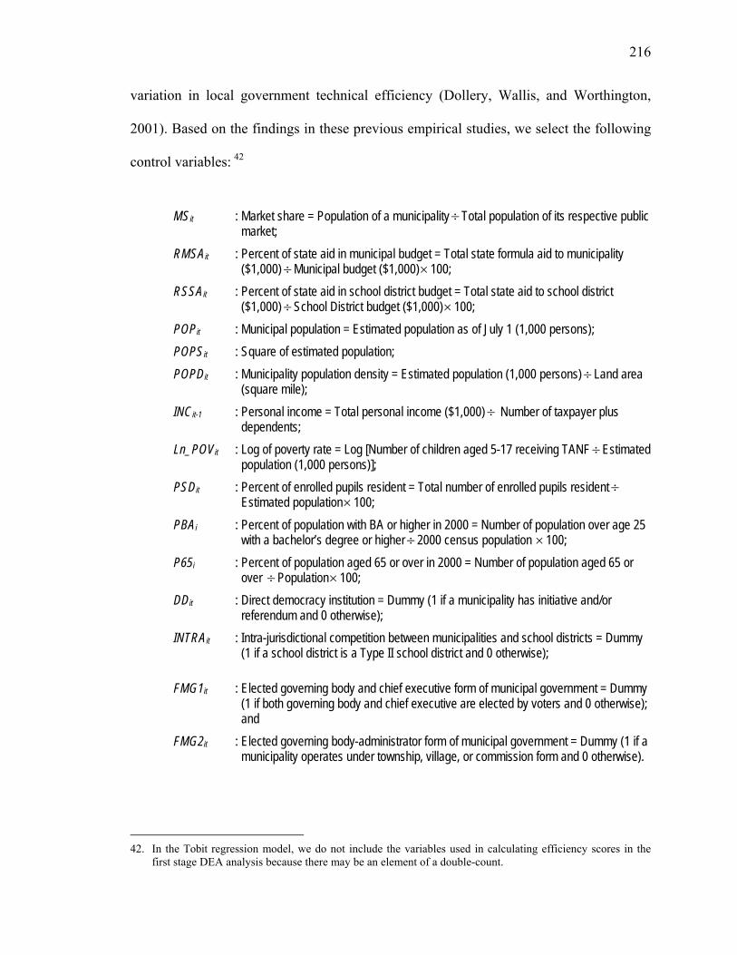
216
variation in local government technical efficiency (Dollery, Wallis, and Worthington,
2001). Based on the findings in these previous empirical studies, we select the following
control variables: 42
MSit : Market share = Population of a municipality÷Total population of its respective public market;
RMSAit : Percent of state aid in municipal budget = Total state formula aid to municipality ($1,000)÷Municipal budget ($1,000)×100;
RSSAit : Percent of state aid in school district budget = Total state aid to school district ($1,000)÷School District budget ($1,000)×100;
POPit : Municipal population = Estimated population as of July 1 (1,000 persons); POPSit : Square of estimated population; POPDit : Municipality population density = Estimated population (1,000 persons)÷ Land area
(square mile); INCit-1 : Personal income = Total personal income ($1,000)÷ Number of taxpayer plus
dependents; Ln_POVit : Log of poverty rate = Log [Number of children aged 5-17 receiving TANF÷Estimated
population (1,000 persons)]; PSDit : Percent of enrolled pupils resident = Total number of enrolled pupils resident÷
Estimated population×100; PBAi : Percent of population with BA or higher in 2000 = Number of population over age 25
with a bachelor’s degree or higher÷ 2000 census population ×100; P65i : Percent of population aged 65 or over in 2000 = Number of population aged 65 or
over ÷Population×100; DDit : Direct democracy institution = Dummy (1 if a municipality has initiative and/or
referendum and 0 otherwise); INTRAit : Intra-jurisdictional competition between municipalities and school districts = Dummy
(1 if a school district is a Type II school district and 0 otherwise);
FMG1it : Elected governing body and chief executive form of municipal government = Dummy (1 if both governing body and chief executive are elected by voters and 0 otherwise); and
FMG2it : Elected governing body-administrator form of municipal government = Dummy (1 if a municipality operates under township, village, or commission form and 0 otherwise).
42. In the Tobit regression model, we do not include the variables used in calculating efficiency scores in the
first stage DEA analysis because there may be an element of a double-count.

217
To capture the potential scale economies in providing local public services,
population (POPit) and population density (POPDit) are included as exploratory variables.
If scale economies are present, it is expected that population and population density are
positively related to technical efficiency. A squared population (POPSit) is included to
account for the deceasing effect of scale economies and thus expected to have a negative
effect on the technical efficiency score.
The share of population aged over 65 (P65i), the number of children receiving
TANF (Ln_POVit), and the share of enrolled resident students (PSDit) are included as a
proxy for the demand for public services. These population groups tend to be heavy users
of local public services. On the other hand, these population structure variables may also
reflect the fiscal capacity of communities. High shares of these population groups
represent the weak fiscal capacity of communities. Whether the share of these population
groups is positively or negatively related to technical efficiency is not clear.43
It is well documented that the income and wealth of residents affect the incentives
of both politicians and taxpayers (De Borger and Kerstens, 1996a, 1996b). Personal
income (INCit-1) is included in the technical efficiency model to control for this effect. A
high level of personal income represents a strong fiscal capacity of communities and may
foster government waste or rent-seeking behaviors (Silkman and Young, 1982). On the
other hand, due to the high opportunity costs of time, the rich may be less motivated to
monitor government performance (De Borger and Kerstens, 1996a, 1996b). Therefore,
personal income (INCit-1) is expected to have a negative impact on technical efficiency.
43. Because the most recent available data on personal income is 2003, a one year lagged variable is used.

218
The education level of residents may also affect the technical efficiency of local
governments. Educated people may be more effective in demanding an efficient
operation of local governments and in monitoring inefficient government behavior. In
addition, the education level may also reflect the effect of a citizen’s political
participation, which is expected to enhance government performance. There is some
evidence that political participation is associated with education level (Mueller, 2003).
Thus, a high level of education increases the pressure on local governments to operate in
a more efficient way (De Borger et al., 1994). The share of the population with a BA or
higher (PBAi) is expected to be positively associated with technical efficiency.
The technical efficiency of local governments may be affected by the institutional
structure of local governments. To control for the effect of these political institutions, we
include a dummy variable for a municipality with direct democracy institutions (DDit), a
dummy variable for a community with a Type II school district (INTRAit), and dummy
variables for the forms of municipal governments (FMG1it and FMG2it). These variables
capture the systematic differences in technical efficiency between different institutional
structures of local governments. We have no prior expectation on the sign of the
influence these political institution variables have on government technical efficiency.
We include the share of state aid in the municipal budget (RMSAit) and in the
school district budget (RSSAit) to capture the effect of a revenue raising system on
technical efficiency because the total amount of state aid to municipalities and school
districts is used an input in the DEA model. The high share of outside funding may
encourage or stimulate inefficient behavior of government officials because the cost of
inefficient behavior is increasingly shared by a broader constituency (Silkman and Young,

219
1982; De Borger and Kerstens, 1996a, 1996b). It is expected that both the share of state
aid in the municipal budget and in the school district budget is negatively related to
technical efficiency.
In addition to the above control variables, the technical efficiency model
incorporates market share (MSit) and time dummy variables. The market share is included
to control for the relative size of each community in the public market. The time dummy
variables are included to control for shocks that are common to all communities but
change from year to year. These shocks may reflect changes in the macro environment
under which local governments operate. We have no prior expectation about the direction
of the effect which the market share and the time dummy variables have on local
government technical efficiency.
4-4. Source of Data and Descriptive Statistics
This section provides information on the source of each actual variable used in the
regression analysis, on any modification of the original data, and descriptive statistics for
each variable. Since the variables are drawn from 566 communities in New Jersey across
several different years and cross-sectional regression analyses use data for the year 2004,
descriptive statistics are provided for all communities for the year 2004 and for all
communities in all the pooled years. The variables described by these statistics are used
in the multiple regression analyses discussed in the next section. Table 4-2 presents the
shorthand name used to identify each variable, its descriptive statistics, and the source of
data.

220
The main sources of data are New Jersey state government, New Jersey
Legislative District Data Book (LDDB), and the U.S. census. The data on property tax
rates, property tax levy, property values, and state aid to municipal governments are
based on Property Tax Tables, Abstract of Ratables, and Property Value Classification
provided by the Division of Local Government Services (NJ DLGS) in the Department of
Community Affairs (NJ DCA). Data on state aid to school districts are gathered from the
Department of Education (NJ DOE). The data on population, land area, population
density, the unemployment rate, and county personal income are taken from the
Department of Labor and Workforce Development (NJ DLWD). The map of New Jersey
municipal boundaries and crime rates are gathered from the Department of
Transportation (NJ DOT).
The institutional structure of local governments such as the form of municipal
government, direct democracy institutions of municipalities, and the Type of school
districts are taken from the LDDB. Some municipal demographic data such as personal
income and poverty rates are also based on the LDDB. Housing characteristics such as
the median number of rooms and the percent of housing built before 1970 come from the
U.S. census of 2000. The percentage of population age over 65, the percentage of adults
with a BA or higher, and the percentage of African-Americans are also gathered from the
U.S. census of 2000. Measures for the degree of inter-jurisdictional competition are
calculated using population data and municipal boundary information.

221
Table 4-2. Descriptive Statistics and Data Source Year 2004 (N=566) Year 2001-04 (N=2264) Variable
Mean SD Min Max Mean SD Min MaxSource of Data 1
Property Tax Rates MTRit 0.514 0.427 0.000 5.666 0.555 0.444 0.000 5.838 DLGS STRit 1.205 0.547 0.000 8.396 1.285 0.507 0.000 8.396 DLGS STRit-1 1.273 0.507 0.000 7.740 1.329 0.486 0.000 7.740 DLGS CTRit 0.427 0.195 0.174 1.032 0.469 0.204 0.163 1.150 DLGS MSTRit 1.719 0.802 0.000 14.062 1.840 0.765 0.000 14.062 DLGS
Property Tax Levy PMTLit-1 0.819 5.469 0.000 129.612 0.793 5.901 0.000 149.519 DLGS PSTLit-1 1.309 0.938 0.000 17.351 1.171 0.742 0.000 17.351 DLGS PCTLit-1 0.631 1.537 0.024 27.882 0.571 1.455 0.024 31.867 DLGS
Property Value TPVit 1,658,953 1,940,553 2,443 12,800,000 1,382,340 1,634,957 0.0 12,800,000 DLGS PCIVit 17.7 13.6 0.0 98.6 18.0 13.5 0.0 98.6 DLGS HOSit 4,254.0 4,967.5 0.0 3,7482.0 4,197.0 4,909.7 0.0 37,482.0 DLGS CIit 247.5 444.4 0.0 6,853.0 247.3 433.4 0.0 6,932.0 DLGS MNRi 6.1 1.0 3.5 8.5 6.1 1.0 3.5 8.5 Census 2000 HB70i 64.0 20.5 6.2 100.0 64.0 20.5 6.2 100.0 Census 2000 LAi 13.1 18.2 0.1 111.3 13.1 18.2 0.1 111.3 DLWD
Budget and State Aid TMBit-1 15,906.7 32,935.2 55.9 553,743.9 15,049.2 30,981.8 42.2 553,743.9 DLGS TSBit-1 16,859.6 19,786.8 0.0 136,229.5 15,151.6 17,963.3 0.0 136,229.5 DLGS PMSAit-1 0.197 0.578 0.061 13.007 0.195 0.571 0.061 13.007 DLGS PSSAit-1 0.463 0.446 0.000 2.544 0.453 0.435 0.000 2.568 DOE MSSAit-1 12,702.5 39,579.5 2.6 57,0277.1 12,310.7 38,212.7 2.6 570,277.1 Calculated RMSAit 13.6 6.2 0.8 42.7 14.4 6.7 0.7 47.8 Calculated RSSAit 26.7 23.3 0.0 100.0 27.8 23.4 0.0 100.0 Calculated
Demographics POPit 15.267 23.102 0.018 277.770 15.150 23.018 0.018 277.770 DLWD POPit-1 15.203 23.073 0.018 276.956 15.058 22.944 0.018 276.956 DLWD POPSit 765.829 4,309.484 0.000 77,156.160 759.127 4,289.975 0.000 77,156.160 Calculated POPSit-1 762.579 4,301.991 0.000 76,704.630 752.912 4,270.242 0.000 76,704.630 Calculated POPDit 3.390 5.099 0.002 56.940 3.386 5.125 0.002 57.499 DLWD POPDit-1 3.389 5.119 0.002 57.204 3.380 5.127 0.002 57.499 DLWD POPGit-1 0.6 1.6 -1.2 17.6 0.7 2.4 -51.6 19.1 Calculated POPCit-1 477.529 253.615 64.433 893.756 472.696 252.678 64.143 893.756 DLWD INCCit-1 40.660 9.002 26.077 56.684 40.084 9.450 23.365 57.241 DLWD PSDit 15.6 4.6 0.000 61.1 15.6 4.6 0.000 83.3 LDDB PSDit-1 15.6 5.0 0.000 83.3 15.5 4.5 0.000 83.3 LDDB
(Continued)

222
Table 4-2. (Continued) Year 2004 (N=566) Year 2001-04 (N=2264) Variable
Mean SD Min Max Mean SD Min MaxSource of Data 1
Demographics (Continued) INCit-1 33.884 21.216 8.832 203.323 33.576 23.934 8.484 232.039 LDDB POVit 2.867 5.202 0.000 46.627 2.788 5.164 0.000 55.556 LDDB POVit-1 2.785 5.169 0.000 46.846 3.101 7.121 0.000 200.000 LDDB RBPit-1 58.3 127.5 0.0 1,652.0 55.8 116.5 0.0 1,652.0 LDDB UERit-1 5.1 2.5 0.0 20.0 4.3 2.3 0.0 20.0 DLWD P65i 14.2 6.1 1.3 54.5 14.2 6.1 1.3 54.5 Census 2000 PBAi 31.2 16.5 0.0 76.1 31.2 16.5 0.0 76.1 Census 2000 PAAi 7.2 12.6 0.0 93.6 7.2 12.6 0.0 93.6 Census 2000 PHOi 73.8 17.9 0.0 97.1 73.8 17.9 0.0 97.1 Census 2000 CRIi 26.1 22.5 0.0 238.3 26.1 22.5 0.0 238.3 DOT
Political Institution DDit 0.293 0.0 1.0 0.294 0.0 1.0 LDDB CONSOLi 0.124 0.0 1.0 0.124 0.0 1.0 LDDB COORDIit 0.035 0.0 1.0 0.034 0.0 1.0 LDDB FMG1it 0.581 0.0 1.0 0.580 0.0 1.0 LDDB FMG2it 0.314 0.0 1.0 0.316 0.0 1.0 LDDB
Measures for Inter-jurisdictional Competition 2 COMit_PM1 0.095 0.058 0.014 0.367 0.096 0.075 0.006 0.625 Calculated COMit_PM2 0.082 0.058 0.012 0.390 0.083 0.059 0.012 0.393 Calculated COMit_PM3 0.102 0.080 0.011 0.614 0.103 0.081 0.011 0.625 Calculated COMit_PM4 0.090 0.052 0.020 0.231 0.091 0.053 0.020 0.234 Calculated MSit_PM1 0.150 0.107 0.000 0.605 0.136 0.097 0.000 0.606 Calculated MSit_PM2 0.064 0.066 0.000 0.555 0.064 0.066 0.000 0.559 Calculated MSit_PM3 0.098 0.128 0.000 0.898 0.097 0.127 0.000 0.901 Calculated MSit_PM4 0.037 0.048 0.000 0.394 0.037 0.048 0.000 0.394 Calculated
Note: 1. DLGS-Division of Local Government Services in Department of Community Affairs; DLWD – Department of Labor and Workforce Development; DOE – Department of Education; DOT – Department of Transportation; LDDB – Legislative District Data Book. 2. PM1 – 1st order contiguity-based public market; PM2 – 2nd order contiguity-based public market; PM3 – Distance-based public market; PM4 – County boundary-based public market.
223
Chapter V. Empirical Results
The previous chapter specified four research models for examining hypotheses.
This chapter presents the results of the statistical analysis of the four research models: the
municipal tax rate model, the combined municipal-school district tax rate model, the
hedonic property value model, and the technical efficiency model. Each research model is
estimated using various multiple regression methods and either 2004 cross-sectional or
2001-2004 panel data for 566 New Jersey communities. The results for all regressions are
summarized in tables 5-2, 5-3, 5-4, and 5-6.
5-1. Existence of Tax Competition
One main purpose of this study is to test whether municipalities compete with
school districts (Hypothesis 1), with counties (Hypothesis 2), and with other neighboring
or competing municipalities (Hypothesis 3) when setting their property tax rates. To test
the hypotheses, this study proceeds in three steps. First, this study examines the spatial
autocorrelation in the dependent variable, municipal property tax rates (MTRit), by
examining a quantile map and via Moran I statistics. Second, to select the proper spatial
model, the non-spatial tax rate model (Equation 1) is estimated and, then, spatial
dependence in the OLS residuals is examined by the LM statistic. Third, the selected
spatial lag or error model is estimated by either the IV or the ML estimation method.
5-1-1. Spatial Autocorrelation Tests on Municipal Property Tax Rates
A. Exploratory Data Analysis by a Quantile Map
We perform a preliminary spatial autocorrelation test on the municipal property
tax rate using a quantile map. Figure 5-1 illustrates the clustering of 2004 municipal,

224
school district, county, and total property tax rates in 2004. In the quantile maps, property
tax rates are sorted and grouped in five categories with equal number of observations. In
the legend, the number of observation in each category is in parentheses. In quantile maps,
high property tax rates municipalities are colored in darker shades of red, while low
municipal property tax rates municipalities are shown in lighter shades of white.
A visual inspection of Figure 5-1 reveals a geographical pattern of municipal
property tax rates. High municipal tax rate communities are concentrated in regions
around Camden city and the north-eastern regions, whereas low property tax rates are
concentrated in the central, north-western, and south-eastern areas. This tendency of high
(low) municipal tax rate communities to be surrounded by other high (low) tax rate
communities provides evidence supporting the presence of spatial dependence in
municipal tax rates.
Figure 5-1 also shows spatial patterns of school districts, counties, and total
property tax rates. High school district tax rate communities are concentrated in the
north-western, middle-western, and around Camden regions, while low school district tax
rate communities are concentrated around the Atlantic coast regions. County tax rates are
clustered by county jurisdictional boundaries and the spatial distributional pattern of total
tax rates are similar to that of school district tax rates.
The quantile map apparently shows that the high municipal tax rate communities
tend to cluster in space and so do the low municipal tax rate communities. Although
cartographic data displays are good tools for exploratory spatial data analysis, it is more
useful to evaluate whether observations are spatially clustered by more formalized tests.
In the following, we perform formal spatial autocorrelation tests on municipal tax rates.
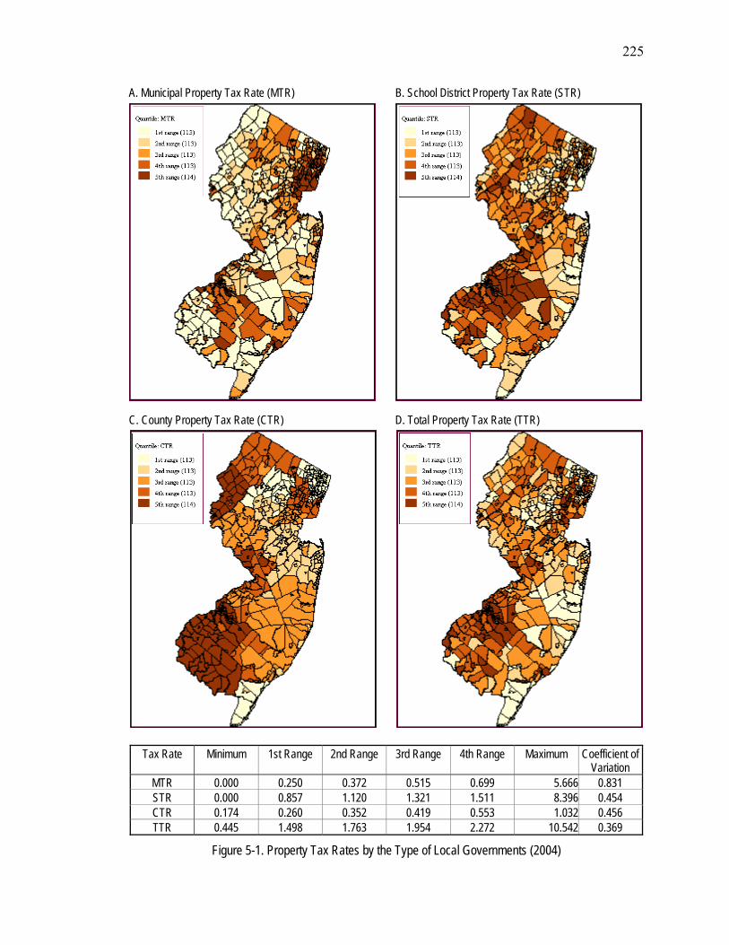
225
A. Municipal Property Tax Rate (MTR) B. School District Property Tax Rate (STR)
C. County Property Tax Rate (CTR) D. Total Property Tax Rate (TTR)
Tax Rate Minimum 1st Range 2nd Range 3rd Range 4th Range Maximum Coefficient of Variation
MTR 0.000 0.250 0.372 0.515 0.699 5.666 0.831 STR 0.000 0.857 1.120 1.321 1.511 8.396 0.454 CTR 0.174 0.260 0.352 0.419 0.553 1.032 0.456 TTR 0.445 1.498 1.763 1.954 2.272 10.542 0.369
Figure 5-1. Property Tax Rates by the Type of Local Governments (2004)

226
B. Formal Test for Spatial Autocorrelation
We test for spatial autocorrelation in municipal property tax rates by the Moran I
spatial autocorrelation statistic and its visualization in the form of a Moran scatter plot.
Figure 5-2 provides the results of the Moran I statistics and the Moran scatter plots.44 The
results confirm the exploratory visual inspection of spatial dependence, showing that
under all four weight matrices, Moran I statistics are statically different from zero. The
Moran I statistics suggest a spatial pattern of positive autocorrelation in municipal
property tax rates.
In the Moran scatter plots, the spatial lag of municipal property tax rates, which is
the simple average property tax rate of neighbors, is shown on the vertical axis, while the
horizontal axis portrays the value of each municipality’s property tax rate. In the scatter
plot, the municipal property tax rates are standardized so that the units on the graph
correspond to standard deviations.
The four quadrants in the graph provide a classification of four types of spatial
autocorrelation: the top right and the bottom left quadrants for positive spatial
autocorrelation; the top left and the bottom right quadrants for negative spatial
autocorrelation. The top right quadrant represents municipalities that have relatively high
property tax rates, surrounded with municipalities that also have high property tax rates.
The bottom left quadrant represents municipalities that have relatively low property tax
rates and are surrounded by municipalities with similarly low property tax rates.
44. Moran I statistics can be calculated based either on randomization or on a normality assumption. Literature
suggests that assuming a normal distribution for the Moran I is often an incorrect assumption (for example, Boots and Tiefelsdorf, 2000). Therefore, the Moran I statistics in Figure 5-2 is calculated based on a random permutation procedure by spdep in R. In the randomization approach, the Moran I statistics are recalculated many times to generate a reference distribution. Then, the calculated statistic is compared to the reference distribution and a significance level is calculated (Anselin, 2005).

227
A. First-order Contiguity B. Second-order Contiguity
C. Euclidean Distance D. County Boundary
Weights Moran I Standard Deviation Variance p-value
First-order Contiguity (W1) 0.2519 9.2423 0.0008 0.0000 Second-order Contiguity (W2) 0.1926 11.6412 0.0003 0.0000 Euclidean Distance (W3) 0.1914 10.038 0.0004 0.0000 County Boundary (W4) 0.1653 15.2002 0.0001 0.0000
Figure 5-2. Moran I Statistics and Moran Scatter Plot for Municipal Property Tax Rates (2004)

228
Figure 5-2 also portrays the OLS regression lines, which produce a summary
measure of the relationship between a municipality’s property tax rate and its
competitors’ average property tax rates. The slopes of the OLS lines are the Moran I
statistics for municipal property tax rates under four different weight matrices
predetermined based on the four criteria in Chapter IV. The calculated Moran Is are
0.2519, 0.1926, 0.1914, and 0.1653, with p values of 0.000. This indicates that there is a
positive spatial dependence in municipal property tax rates under all four definitions of
public market.
5-1-2. Spatial Regression Analysis
A. Spatial Autocorrelation Test on OLS Residuals
To determine the proper spatial model, we use LM and robust LM tests on the
OLS residuals of the non-spatial municipal tax rate model (Equation 1). As suggested in
Chapter IV, the county property tax rate (CTRit) and the school district property tax rate
(STRit) are suspected to be endogenous. To solve the endogeneity issue, we first regress
county and school district tax rates on exogenous explanatory variables and three
instrumental variables. The instruments are one year lagged school district tax rates
(STRit-1), one year lagged county population (POPCit-1), one year lagged county property
tax levy (PCTLit-1), and one year lagged county personal income (INCCit-1). In the second
stage, the fitted values of county property tax rates (CTRit_HAT) and school district
property tax rates (STRit_HAT) are used in Equation 1 to obtain OLS residuals.45
45. This process is done manually because the spatial regression package spdep in R does not have a built-in
function for IV or 2SLS estimation. Although the manually calculated OLS residuals are different from those produced by the installed function for IV or 2SLS in STATA, the correlation coefficient between them is over 0.96. The outputs of the first stage regression are provided in Appendix A.

229
We calculate, for each of the four weight matrices, LM test statistics on the OLS
residuals of the non-spatial municipal tax rate model. Based on LM and robust LM
statistics, we conclude that a spatial lag model is the proper spatial model under the first-
order contiguity, the second-order contiguity, and the Euclidean distance weights
matrices, while a spatial error model is the preferred model under the county boundary
weight matrix. Table 5-1 reports five LM statistics by weight matrix.
Under both the first-order contiguity and the Euclidean distance weight matrices,
the LM lag statistics are statistically significant (p = 0.009 and 0.03, respectively) while
the LM error statistics are not significant (p = .122 and .437, respectively). On the other
hand, both LM error and LM lag statistics are statistically significant under the second-
order contiguity weight matrix. Of the robust forms, the robust LM lag statistic is
significant (p = .004), but the robust LM error is insignificant (p = .45). As a result, it is
concluded that spatially lagged dependent variable is the relevant source of spatial
dependence when we define a public market based on the first-order contiguity, the
second-order contiguity, and the Euclidean distance.
However, a spatial error model is identified as the proper model under the county
boundary-based weight matrix. Although robust LM statistics both for spatial lag
dependence and for spatial error dependence are statistically significant, the robust LM
error statistics (15.197 with p value of 0.000) is greater and more statistically significant
than the robust LM lag statistic (3.876 with p value of 0.049). This indicates that the
spatial dependence is caused by spatially lagged errors. However, unlike under other
weight matrices, the robust LM lag statistic is still highly significant. This suggests that

230
spatial dependence exists both in the dependent variable and in the error term and, thus,
the proper model may be a spatially autoregressive and moving average (SARMA) model.
Table 5-1. Spatial Autocorrelation in Residuals of the Non-spatial Municipal Tax Rate Model
Weight Matrix: W1 W2 W3 W4
LM for Spatial Lag Dependence 6.851 (0.009) 19.242 (0.000) 4.738 (0.030) 22.562 (0.000)
LM for Spatial Error Dependence 2.394 (0.122) 11.354 (0.001) 0.605 (0.437) 33.884 (0.000)
Robust LM for Spatial Lag Dependence 4.856 (0.028) 8.460 (0.004) 5.097 (0.024) 3.876 (0.049)
Robust LM for Spatial Error Dependence 0.399 (0.528) 0.571 (0.450) 0.964 (0.326) 15.197 (0.000)
LM for SARMA 7.250 (0.027) 19.813 (0.000) 5.702 (0.058) 37.760 (0.000) Weights matrices: W1=First order contiguity, W2=Second order contiguity, W3=Distance weights, and W4=County weights
B. Spatial Regression Analysis
This sub-section presents the results of regression analysis examining the
existence of inter-municipal competition and intra-jurisdictional competition between
municipalities and school districts and between municipalities and counties in setting
property tax rates. Based on the LM tests, we identified proper spatial models between
the spatial lag and the spatial error models. The selected spatial lag model or the spatial
error model is estimated using data on property tax rates of 566 New Jersey
municipalities in 2004.
Table 5-2 reports the regression results of the municipal tax rate models (Equation
1, 2, and 3). The first column presents the two-step IV estimation results of the non-
spatial municipal tax rate model whose residuals are used to compute the LM statistics.In
the columns from second to fourth, we present the Baum, Schaffer, and Stillman’s (2007)
IV GMM estimation results of the spatial lag municipal tax rate models. The Kelejian and
Prucha’s (1999) GMM estimation results of the spatial error municipal tax rate model are
reported in the fifth column.

231
a. Spatial lag model
As we discussed in the Chapter IV, the spatially lagged dependent variable
(WMTRit), school district tax rates (STRit), and county tax rates (CTRit) are endogenous.
In order to solve the endogeneity issue, we can use either the IV or the ML method in
estimating the spatial lag model. We use the IV approach since the ML estimation
method cannot be used when explanatory variables other than the spatially lagged
dependent variable are endogenous. The estimation of the spatial lag model is
implemented by the Baum, Schaffer, and Stillman’s (2007) IV GMM estimation method
in Stata.
The IV regression results of the spatial lag tax rate setting model (Equation 2)
show that Hansen’s J of over-identification, Kleibergen-Paap of under-identification, and
F-values of first stage regressions do not reject the validity of the instrument variables
with a reasonable degree of confidence. However, Breusch-Pagan and Pagan-Hall tests
show that heteroskedasticity is present. The Huber-White-sandwich estimator of variance
is used to produce valid standard errors in the presence of heteroskedasticity. The outputs
of first stage regression for spatially lagged dependent variable, school district tax rates,
and county tax rates are presented in Appendix B.46
b. Spatial error model
The spatial error model (Equation 3) is estimated by Kelejian and Prucha’s (1999)
GMM approach which is consistent even with the non-normality of the error term. Since 46. The list of instruments for the three endogenous variables include all exogenous regressors, one year lagged
school district tax rates (STRit-1), one year lagged county population (POPCit-1), one year lagged county property tax levy (PCTLit-1), one year lagged county personal income (INCCit-1), and spatially lagged variables of municipal property tax levy (PMTLit-1), municipal population (POPit_1), square of municipal population (POPSit_1), municipal population density (POPDit_1), poverty rate (POVit_1), residential building permits (POVit_1), percent of African-American population (PAAit-4), percent of population age over 65 (P65it-4), percent of homeownership (PHOit-4), and crime rate (CRIit-4).

232
the Jarque-Bera test on residuals of the non-spatial municipal tax rate model (Equation 1)
rejects the null hypothesis of a normally distributed error term (27,804.64 with p-value of
0.000), we cannot estimated the spatial error model by the ML estimation method. In
addition, the IV approach is not appropriate for obtaining a consistent estimator for the
spatial autocorrelation coefficient in a spatial error model (Kelejian and Prucha, 1997).
The results of the spatial error model estimated by GMM shows that the spatial
autoregressive error coefficient is estimated as 0.409, and is highly significant. This
indicates that the spatial dependence in the municipal tax rates is caused by the spatially
autocorrelated omitted variables. The results also show that the spatial error model
performs better than the non-spatial municipal tax rate model. If we compare the values
for the spatial error model in column 5 to those in column 1, we notice an increase in the
Log-Likelihood from -65.4 for the non-spatial model to -55.3 for spatial error model by
GMM.
C. Existence of Intra-jurisdictional Competition
The regression results of the municipal tax rate models provide strong evidence
supporting both Hypothesis 1 and Hypothesis 2, showing that the coefficient on the
school district tax rates (STRit) and the county tax rates (CTRit) are highly significant
across the four weight matrices. However, the municipality responds differently to tax
rates of school districts and counties. While county tax rates have a negative effect on the
municipal property tax rates, the school district property tax rates are positively related to
the municipal tax rates.
The consistently positive and significant coefficients of school district tax rates
across four different weight matrices suggests that municipal and school district property

233
tax rates are strategic complements: an increase in the school district tax rate leads to
increases in the municipal tax rate. The estimated coefficients suggest that $1 increase in
the school district property tax rate induces the municipality to increase its property tax
rate by $0.190 - $0.387.
The consistently negative and significant coefficient of county tax rates across
four weight matrices indicates that municipal governments decrease their tax rates in
reaction to an increase in county property tax rates. The estimated coefficients indicate
that $1 increase in the county property tax rate leads to a fall of $0.273 - $0.382 in the
municipal government property tax rate. The results can be explained such that a higher
county tax rate makes it more difficult for the municipalities to raise revenues from the
same base.
D. Existence of Inter-jurisdictional Competition
The IV regression results of the spatial lag model confirm Hypothesis 3, showing
that the coefficients on the spatially lagged dependent variable (WMTRit) are statistically
significant under the first-order contiguity, the second-order contiguity, and the Euclidean
distance weight matrices. The estimated coefficients on the spatially lagged dependent
variable (WMTRit) indicate that municipalities do behave strategically with other
neighboring or competing municipalities in setting property tax rates. Under three
different weight matrices, the estimated coefficients suggest that a municipality would
respond to a $1 increase in its neighbors’ tax rates by raising its tax rates between about
$0.205 and $0.286.
As stated above, it is suggested that the proper spatial model may be the SARMA
model under county boundary-based weight matrix. We test whether both coefficients on

234
the spatially lagged dependent variable and the spatially lagged error term are
significant.47 The results of the SARMA model confirm Hypothesis 3, showing that both
coefficients on the spatial lag and spatial error are highly significant. The results also
mean that when we define the public market based on the county boundary, the proper
model may be the SARMA model. The regression output of the SARMA model is
presented in Appendix C.
E. Control Variables
The coefficients of control variables generally show the expected signs and are
consistent in terms of their sign and statistical significance across four different weight
matrices. Although the coefficient of the dummy for the elected governing body-
administrator form of municipal government (FMG2it) shows different signs across four
weight matrices, it is not statistically significant at the conventional significance level.
The unemployment rate (UERit) and the dummy for school district consolidation
(CONSOLit) do not have any statistically significant effects on municipal tax rates across
all weight matrices.
The regression results shows that while population (POPit-1) and population
density (POPDit-1) have consistent positive effects, squared population (POPSit-1) has
consistent negative effect. This indicates that decreasing economies of scale are present
in the provision of public goods. The per capita property tax levy (PMTLit-1), the poverty
rate (POVit-1), personal income (INCit-1), and the percent of African Americans (PAAit-4) 47. For estimating the SARMA tax rate setting model, we first regress the spatially lagged dependent variable
(WMTRit), school district tax rates (STRit), and county tax rates (CTRit) on the spatially lagged variables of exogenous exploratory variables (WXit-k), county and school district demographic variables, and all exogenous exploratory variables (Xit-k). Then, the fitted values of spatially lagged dependent variable (WMTRit_HAT), county property tax rates (CTRit_HAT), and school district property tax rates (STRit_HAT) are used to estimate the spatial error tax rate setting model by using Kelejian and Prucha’s (1999) GMM in spdep package in R.

235
have consistent positive effects on municipal tax rates. The number of residential
building permits (RBPit-1) and the percent of the population with a BA or higher degree
(PBAit-4) are negatively related to municipal property tax rates across all weight matrices.
The percent of senior population (P65it-4), the crime rate (CRIit-4), a dummy for
elected governing body and the chief executive form of municipal government (FMG1it),
and a dummy for direct democracy institution of municipal government (DDit) have
consistent positive effects but statistically significant under only some weight matrices.
The percent of home ownership (PHOit-4) and a dummy for the municipality with the
Type II school district (INTRAit) are negatively related to municipal tax rates but the
statistical significance differs by the weight matrix.
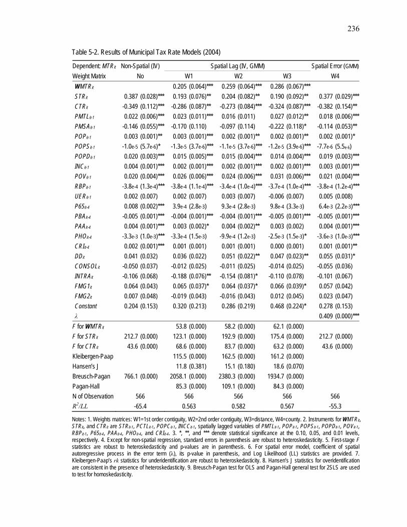
236
Table 5-2. Results of Municipal Tax Rate Models (2004)
Dependent: MTRit Non-Spatial (IV) Spatial Lag (IV, GMM) Spatial Error (GMM) Weight Matrix No W1 W2 W3 W4 WMTRit 0.205 (0.064)*** 0.259 (0.064)*** 0.286 (0.067)*** STRit 0.387 (0.028)*** 0.193 (0.076)** 0.204 (0.082)** 0.190 (0.092)** 0.377 (0.029)*** CTRit -0.349 (0.112)*** -0.286 (0.087)** -0.273 (0.084)*** -0.324 (0.087)*** -0.382 (0.154)** PMTLit-1 0.022 (0.006)*** 0.023 (0.011)*** 0.016 (0.011) 0.027 (0.012)** 0.018 (0.006)*** PMSAit-1 -0.146 (0.055)*** -0.170 (0.110) -0.097 (0.114) -0.222 (0.118)* -0.114 (0.053)** POPit-1 0.003 (0.001)** 0.003 (0.001)*** 0.002 (0.001)** 0.002 (0.001)** 0.002 (0.001)* POPSit-1 -1.0e-5 (5.7e-6)* -1.3e-5 (3.7e-6)*** -1.1e-5 (3.7e-6)*** -1.2e-5 (3.9e-6)*** -7.7e-6 (5.5e-6) POPDit-1 0.020 (0.003)*** 0.015 (0.005)*** 0.015 (0.004)*** 0.014 (0.004)*** 0.019 (0.003)*** INCit-1 0.004 (0.001)*** 0.002 (0.001)*** 0.002 (0.001)*** 0.002 (0.001)*** 0.003 (0.001)*** POVit-1 0.020 (0.004)*** 0.026 (0.006)*** 0.024 (0.006)*** 0.031 (0.006)*** 0.021 (0.004)*** RBPit-1 -3.8e-4 (1.3e-4)*** -3.8e-4 (1.1e-4)*** -3.4e-4 (1.0e-4)*** -3.7e-4 (1.0e-4)*** -3.8e-4 (1.2e-4)*** UERit-1 0.002 (0.007) 0.002 (0.007) 0.003 (0.007) -0.006 (0.007) 0.005 (0.008) P65it-4 0.008 (0.002)*** 3.9e-4 (2.8e-3) 9.3e-4 (2.8e-3) 9.8e-4 (3.3e-3) 6.4e-3 (2.2e-3)*** PBAit-4 -0.005 (0.001)*** -0.004 (0.001)*** -0.004 (0.001)*** -0.005 (0.001)*** -0.005 (0.001)*** PAAit-4 0.004 (0.001)*** 0.003 (0.002)* 0.004 (0.002)** 0.003 (0.002) 0.004 (0.001)*** PHOit-4 -3.3e-3 (1.0e-3)*** -3.3e-4 (1.5e-3) -9.9e-4 (1.2e-3) -2.5e-3 (1.5e-3)* -3.6e-3 (1.0e-3)*** CRIit-4 0.002 (0.001)*** 0.001 (0.001) 0.001 (0.001) 0.000 (0.001) 0.001 (0.001)** DDit 0.041 (0.032) 0.036 (0.022) 0.051 (0.022)** 0.047 (0.023)** 0.055 (0.031)* CONSOLit -0.050 (0.037) -0.012 (0.025) -0.011 (0.025) -0.014 (0.025) -0.055 (0.036) INTRAit -0.106 (0.068) -0.188 (0.076)** -0.154 (0.081)* -0.110 (0.078) -0.101 (0.067) FMG1it 0.064 (0.043) 0.065 (0.037)* 0.064 (0.037)* 0.066 (0.039)* 0.057 (0.042) FMG2it 0.007 (0.048) -0.019 (0.043) -0.016 (0.043) 0.012 (0.045) 0.023 (0.047) Constant 0.204 (0.153) 0.320 (0.213) 0.286 (0.219) 0.468 (0.224)* 0.278 (0.153) λ 0.409 (0.000)***
F for WMTRit 53.8 (0.000) 58.2 (0.000) 62.1 (0.000) F for STRit 212.7 (0.000) 123.1 (0.000) 192.9 (0.000) 175.4 (0.000) 212.7 (0.000) F for CTRit 43.6 (0.000) 68.6 (0.000) 83.7 (0.000) 63.2 (0.000) 43.6 (0.000) Kleibergen-Paap 115.5 (0.000) 162.5 (0.000) 161.2 (0.000) Hansen’s J 11.8 (0.381) 15.1 (0.180) 18.6 (0.070) Breusch-Pagan 766.1 (0.000) 2058.1 (0.000) 2380.3 (0.000) 1934.7 (0.000) Pagan-Hall 85.3 (0.000) 109.1 (0.000) 84.3 (0.000) N of Observation 566 566 566 566 566 R2/LL -65.4 0.563 0.582 0.567 -55.3
Notes: 1. Weights matrices: W1=1st order contiguity, W2=2nd order contiguity, W3=distance, W4=county. 2. Instruments for WMTRit, STRit, and CTRit are STRit-1, PCTLit-1, POPCit-1, INCCit-1, spatially lagged variables of PMTLit-1, POPit-1, POPSit-1, POPDit-1, POVit-1, RBPit-1, P65it-4, PAAit-4, PHOit-4, and CRIit-4. 3. *, **, and *** denote statistical significance at the 0.10, 0.05, and 0.01 levels, respectively. 4. Except for non-spatial regression, standard errors in parenthesis are robust to heteroskedasticity. 5. First-stage F statistics are robust to heteroskedasticity and p-values are in parenthesis. 6. For spatial error model, coefficient of spatial autoregressive process in the error term (λ), its p-value in parenthesis, and Log Likelihood (LL) statistics are provided. 7. Kleibergen-Paap’s rk statistics for underidentification are robust to heteroskedasticity. 8. Hansen’s J statistics for overidentification are consistent in the presence of heteroskedasticity. 9. Breusch-Pagan test for OLS and Pagan-Hall general test for 2SLS are used to test for homoskedasticity.

237
5-2. Effect of Competition on Property Tax Rates
This section presents the results of the combined municipal-school district tax rate
model (Equation 4) examining the effects of inter-jurisdictional competition (Hypothesis
4), market share (Hypothesis 7), school district consolidation (Hypothesis 8), and intra-
jurisdictional competition (Hypothesis 11) on property tax rates. The combined tax rate
model is estimated using the Generalized Estimating Equations (GEE) method and data
on 566 communities in New Jersey for the years 2001 to 2004. The regression results
provide evidence supporting Hypothesis 4, Hypothesis 8, and Hypothesis 11, but little
evidence of asymmetric tax competition (Hypothesis 7).
A. Overview of the Regression Results
The regression diagnostics show that there is evidence of severe first order serial
correlation and heteroskedasticity. The Wooldridge’ first order serial correlation test for
panel data show that we cannot reject the null hypothesis under all four definitions of a
public market. Furthermore, the Breusch-Pagan test for heteroskedasticity indicates that
the error term is heteroskedastic under all four definitions of public market. To overcome
these two issues, we estimate the combined tax rate model by using the GEE method.48
Alternatively, we also estimate the combined tax rate model by a random-effects
model with Rogers’ standard errors which are robust to heteroskedasticity and
autocorrelation. The regression outputs of the random-effects estimation are provided in
48. The literature provides several alternative methods such as panel-corrected standard errors (PCSEs) and
feasible generalized least squares (FGLS) for panel data as the solution to serial correlation and heteroskedasticity (Beck and Katz, 1995). These methods, however, work best when the number of time points is greater than the number of cross-sections or panels. Because this study analyzes property tax rates of 566 communities from 2001-2004, the number of panels is much greater than the number of time points, so PCSEs and FGLS are not appropriate.

238
Appendix D. The results are consistent across the two estimation methods with an
exception of the coefficient on the dummy variable for communities with the Type II
school district (INTRAit). Although the signs of coefficients on population (POPit-1),
population density (POPDit-1), and the percent of student (PSDit-1) are not consistent
between the GEE and the random-effects with Rogers standard errors approach, all of
them are not statistically different from zero.
B. Effect of Inter-jurisdictional Competition
The results of the combined tax rate model provide strong evidence supporting
Hypothesis 4 that the degree of inter-jurisdictional competition has a negative effect on
the property tax rate. The estimated coefficient of the degree of inter-jurisdictional
competition (COMit) is negative and statistically significant across all four definitions of
a public market. The coefficient indicates that an increase in governmental units per 1000
persons reduces the combined municipal-school district property tax rate by $0.421 –
$2.128. The results are consistent with the theoretical prediction of four inter-
jurisdictional competition theories that inter-jurisdictional competition leads to lower tax
rates.
C. Effect of Market Share
The regression results of the combined municipal-school district tax rate model
show little evidence to support the theoretical argument from asymmetric tax competition
that relatively larger jurisdictions tend to have higher tax rates than smaller competing
jurisdictions (Hypothesis 7). While the market share (MSit) has an expected positive and
statistically significant effect on the combined tax rate under the second-order contiguity

239
based a public market, it has negative but not statistically significant effect under all other
definitions of a public market.
D. Effect of Local Government Consolidation
The results of the combined tax rate model provide strong evidence supporting the
school district consolidation hypothesis (Hypothesis 8) that the property tax rate is lower
in the community which is a member of a consolidated school district. The coefficient on
the dummy variable for school district consolidation (CONSOLi) is negative and
statistically significant at the 10% significance level under all four definitions of a public
market. The estimated coefficients indicate that the property tax rates in the community
which is a member of a consolidated school district are lower by about $0.118 – $0.136
than in the community with a regular school district. This supports Oates’ (1972) view
that small government consolidation is associated with lower tax rates due to economies
of scale, while rejecting the tax competition theory that the mergers of small jurisdiction
results in higher tax rates.
E. Intra-jurisdictional Competition v.s. Budget Referendum
Because the dummy variable for the intra-jurisdictional competition (INTRAit)
reflects two institutions of the budget referendum and the intra-jurisdictional competition
and their effects are opposite, we develop a conditional hypothesis about the effect of
intra-jurisdictional competition on the tax rate. The econometric results of the combined
tax rate model provide evidence supporting the dominance of the budget referendum
effect that property tax rates are lower in communities with Type II school districts if the

240
budget referendum effect outweighs the intra-jurisdictional competition effect
(Hypothesis 11).
The coefficient on the communities with Type II school districts (INTRAi) is
positive and statistically significant under all four definitions of a public market. The
estimated coefficients indicate that property tax rates in the community with the Type II
school district are lower by about $1.096 – $1.102 than in the communities with the Type
I school district. However, this result is not confirmed by the results of random-effects
estimation, which shows that the coefficient is never statistically significant under all four
definitions of a public market (see Appendix D).
F. Control Variables
Most control variables have the expected effects on the combined tax rates and
are statistically significant at the conventional level. In addition, the coefficients of
control variables are consistent across four definitions of a public market. No coefficients
are positive and significant in one definition of public market but negative and significant
in another definition. However, state aid to school districts per capita (PSSAit-1),
population density (POPDit-1), personal income (INCit-1), the percent of resident pupils
(PSDit-1), and the dummy for direct democracy institution of municipality (DDit) are
never significant across the four definitions of a public market.
The log of municipal property tax levy per capita (PMTLit-1), the log of school
district property tax levy per capita (PSTLit-1), the log of poverty rate (Ln_POVit-1), and
the percent of African-Americans (PAAi) have positive and statistically significant effects
on the combined tax rates across the four definitions of a public market. On the other

241
hand, state aid to municipalities per capita (PMSAit-1), the number of residential building
permits (RBPit-1), the unemployment rate (UERit-1), the percent of seniors (P65i), the
percent of population with a BA or higher (PBAi), the percent of homeownership
(PHOi),and the dummy for the elected governing body and chief executive form of
municipal government (FMG1it) have negative and statistically significant effects on the
combined tax rates under the four definitions of public market.
The effect of population (POPit-1) differs by the definition of a public market. The
coefficient in positive under county boundary-based public market but it is negative in all
other definitions of public market. However, the coefficient is not statistically different
from zero with the exception of the second-order contiguity based public market. The
coefficients of dummy variables for years are negative and statistically significant across
all definitions of public market. As shown in Chapter II, the downward trend of property
tax rates throughout the period may be caused by the consistent increase in property
values.

242
Table 5-3. Results of Combined Municipal-School District Tax Rate Model by GEE (2001-2004) Public Market Dependent Variable:
MSTRit PM1 PM2 PM3 PM4 COMit -0.421 (0.243)* -2.128 (0.616)*** -1.475 (0.495)*** -1.792 (0.888)** MSit -0.074 (0.120) 0.701 (0.326)** -0.269 (0.166) -0.827 (0.688) CONSOLi -0.128 (0.072)* -0.125 (0.070)* -0.118 (0.068)* -0.136 (0.075)* INTRAit -1.096 (0.547)** -1.102 (0.556)** -1.096 (0.558)** -1.097 (0.557)** CTRit 0.943 (0.122)*** 0.973 (0.132)*** 0.966 (0.132)*** 0.967 (0.130)*** Ln_PMTLit-1 0.076 (0.024)*** 0.074 (0.023)*** 0.065 (0.021)*** 0.075 (0.022)*** Ln_PSTLit-1 0.276 (0.081)*** 0.274 (0.086)*** 0.261 (0.086)*** 0.270 (0.085)*** PMSAit-1 -0.185 (0.066)*** -0.181 (0.066)*** -0.175 (0.067)*** -0.187 (0.066)*** PSSAit-1 0.141 (0.097) 0.129 (0.098) 0.148 (0.099) 0.147 (0.098) POPit-1 -2.9e-4 (1.1e-3) -0.002 (0.001)* -7.4e-4 (1.2e-3) 3.5e-4 (2.1e-3) POPDit-1 0.001 (0.010) -0.002 (0.011) -0.004 (0.011) -0.004 (0.011) INCit-1 -0.002 (0.002) -0.002 (0.002) -0.002 (0.002) -0.002 (0.002) Ln_POVit-1 0.022 (0.009)** 0.023 (0.009)** 0.023 (0.009)** 0.023 (0.009)** RBPit-1 -6.8e-5 (3.5e-5)* -7.8e-5 (3.4e-5)** -7.1e-5 (3.5e-5)** -6.8e-5 (3.5e-5)* UERit-1 -0.044 (0.012)*** -0.042 (0.013)*** -0.042 (0.013)*** -0.041 (0.013)*** PSDit-1 0.003 (0.007) 0.004 (0.007) 0.004 (0.007) 0.004 (0.007) P65i -0.024 (0.006)*** -0.024 (0.006)*** -0.024 (0.006)*** -0.025 (0.006)*** PBAi -0.012 (0.003)*** -0.013 (0.003)*** -0.013 (0.003)*** -0.013 (0.003)*** PAAi 0.008 (0.004)** 0.008 (0.004)** 0.007 (0.004)** 0.008 (0.004)** PHOi -0.012 (0.007)* -0.011 (0.007)* -0.011 (0.007)* -0.012 (0.007)* CRIi -0.006 (0.002)** -0.006 (0.002)** -0.006 (0.002)** -0.006 (0.003)** DDit -0.031 (0.032) -0.029 (0.031) -0.015 (0.030) -0.024 (0.032) FMG1it -0.078 (0.038)** -0.072 (0.038)* -0.081 (0.037)** -0.088 (0.038)** FMG2it -0.204 (0.097)** -0.165 (0.102) -0.145 (0.109) -0.177 (0.106)* Year 2002 -0.028 (0.009)*** -0.030 (0.009)*** -0.029 (0.009)*** -0.030 (0.009)*** Year 2003 -0.047 (0.023)** -0.051 (0.025)** -0.049 (0.024)** -0.052 (0.025)** Year 2004 -0.133 (0.028)*** -0.140 (0.030)*** -0.136 (0.030)** -0.140 (0.030)*** Constant 4.603 (0.844)*** 4.695 (0.858)*** 4.686 (0.854)*** 4.775 (0.891)***
Autocorrelation 52.2 (0.000) 49.7 (0.000) 49.6 (0.000) 47.7 (0.000) Heteroskedasticity 1542.0 (0.000) 1612.8 (0.000) 1687.0 (0.000) 1748.5 (0.000) N of Observation 2264 2264 2264 2264 Wald x2 1253.0 (0.000) 1132.9 (0.000) 1169.1 (0.000) 1127.7 (0.000) Notes: 1. *, **, and *** denote statistical significance at the 0.10, 0.05, and 0.01 levels, respectively. 2. Standard errors robust to first order autocorrelation and heteroskedasticity are in parenthesis. 3. Breusch-Pagan test for heteroskedasticity is based on pooled-OLS and p-values are in parenthesis. 4. Serial correlation is tested by Wooldridge test for panel data and p-values are in parenthesis.
243
5-3. Effect of Competition on Allocative Efficiency
This section provides the regression results of the hedonic property value model
(Equation 5) examining the effect of inter-jurisdictional competition (Hypothesis 5),
school district consolidation (Hypothesis 9), and intra-jurisdictional competition
(Hypothesis 12) on local government allocative efficiency. Using data on 566
communities in New Jersey in 2004, the hedonic property value model is estimated by
OLS and the standard error of the estimates is corrected due to the heteroskedastic error
term.49 The OLS results of the hedonic property value model provide strong evidence of
Hypothesis 12, some evidence of Hypothesis 5, and no evidence of Hypothesis 9.
A. Effect of Inter-jurisdictional Competition
The OLS regression results of the hedonic property value model presented in
Table 5-4 provide some evidence supporting the hypothesis that inter-jurisdictional
competition has an impact on government allocative efficiency (Hypothesis 5). The
coefficient on the number of municipalities within a public market per 1000 persons
(COMit) is positive across four definitions of a public market but statistically significant
under public markets defined by the first-order contiguity and the county boundary. The
coefficient indicates that 1% increase in COMit is associated with a 0.085% – 0.109%
increase in the total equalized property value of a community.
There are two contrasting perspectives on the effect of inter-jurisdictional
competition on government allocative efficiency. While Tiebout, the Leviathan
hypothesis, and the yardstick competition theory suggest that inter-jurisdictional
49. The model is also estimated by the GEE and the random-effects model with Rogers standard errors using a
panel data set for the period from 2001-2004 (see Appendix E and F).

244
competition makes local governments responsive and accountable to the public interests,
the conventional tax competition theory formally demonstrates that inter-jurisdictional
competition results in allocative inefficiency. Although the statistical significance of the
coefficient differs by the definition of public market, the findings provide some evidence
supporting the optimistic view on inter-jurisdictional competition that competition among
local governments enhances government allocative efficiency.
B. Effect of School District Consolidation
The OLS results of the hedonic property value model provide no evidence of the
school district consolidation hypothesis that there is a difference in allocative efficiency
between communities which are member of a consolidated school district and
communities with the regular school district (Hypothesis 9). Although the coefficient on
the dummy variable for school district consolidation (CONSOLit) is negative as expected,
it is not statistically different from zero under the four definitions of a public market.
C. Intra-jurisdictional Competition v.s. Budget Referendum
The OLS results of the hedonic property model also provide strong evidence
supporting the dominance of budget referendum effects that allocative efficiency is
higher in communities with Type II school districts if the budget referendum effect
outweighs the intra-jurisdictional competition effect (Hypothesis 12). The coefficient on
the dummy for communities with Type II school districts (INTRAit) is positive and
statistically significant under the four definitions of a public market. The estimated
coefficient can be interpreted as suggesting that, on average, the equalized property

245
values of a community with the Type II school district are higher than a community with
the Type I school district by about $14,500 - $16,700.
D. Control Variables
The OLS results of the hedonic property value model are highly consistent across
four definitions of a public market, in terms of the sign, the magnitude, and the statistical
significance of coefficients. The one exception is market share (MSit), but its coefficient
is not statistically different from zero under all definitions of public market. Furthermore,
the coefficients of control variables retain the expected signs with the exceptions of the
log of state aid to municipalities and school districts (Ln_MSSAit-1), the log of median
number of rooms (Ln_MNRit-4), and the log of the crime rate (Ln_CRIit-4). However, the
latter two variables are not statistically significant at the conventional confidence level.
Contrary to expectations, the coefficient on state aid is negative and statistically
significant under all definitions of a public market. This may be explained by the
calculation of state aid to school districts, which is inversely related to the equalized
value of taxable property. In addition, the results are consistent with other studies
estimating the Brueckner’s (1979, 1982) model such as Brueckner (1982), Deller (1990),
Taylor (1995), and Bates and Santerre (2003).
The results in Table 5-4 show that while the log of housing stocks (Ln_HOSit), the
log of personal income (Ln_INCit-1), and the log of residential building permits
(Ln_RBPit-1) have consistent positive effects, the log of percent of housing built before
1970 (Ln_HB70it-4), population growth (POPGit-1), and the log of poverty rate
(Ln_POVit-1) have the opposite effect on the property value. However, the log of

246
commercial and industrial property value share (PCIVit), the log of population density
(Ln_POPDit-1), the log of unemployment rate (Ln_UERit-1), the dummy for direct
democracy institution of municipalities (DDit), and two dummies for the form of
municipal government (FMG1it and FMG2it) have no statistically significant effects on
the property value.
One of the important regression results found in Table 5-4 is the estimated
coefficients on the log of municipal expenditures (Ln_TMBit-1) and the log of school
district expenditures (LN_TSBit-1). The empirical results show that both coefficients are
consistently significant and positive across four definitions of a public market, indicating
that an increase in the level of either of these public goods has a positive effect on the
total equalized property value.
According to the Brueckner’s (1979, 1982) thesis, significant positive
coefficients on expenditures indicate that public goods are not systematically
overprovided, while significantly negative coefficients indicate that the public goods are
not systematically underprovided. Therefore, the results provide evidence that public
service provided by municipalities and education services are not being systematically
overprovided and may indeed be underprovided in New Jersey.

247
Table 5-4. Results of Hedonic Property Value Model by OLS (2004)
Public Market Dependent Variable: Ln_TPVit PM1 PM2 PM3 PM4
Ln_COMit 0.109 (0.058)* 0.009 (0.058) 0.041 (0.043) 0.085 (0.033)**
Ln_MSit -0.044 (0.050) 0.023 (0.053) -0.016 (0.035) -0.044 (0.033)
CONSOLit -0.006 (0.037) -0.012 (0.038) -0.009 (0.037) -0.004 (0.037)
INTRAit 0.156 (0.078)** 0.167 (0.080)** 0.164 (0.079)** 0.145 (0.080)*
Ln_TMBit-1 0.795 (0.063)*** 0.783 (0.064)*** 0.781 (0.061)*** 0.785 (0.060)***
Ln_TSBit-1 0.070 (0.024)*** 0.066 (0.022)*** 0.068 (0.023)*** 0.071 (0.024)***
Ln_MSSAit-1 -0.175 (0.028)*** -0.200 (0.029)*** -0.188 (0.027)*** -0.172 (0.026)***
Ln_HOSit 0.344 (0.053)*** 0.322 (0.051)*** 0.342 (0.051)*** 0.351 (0.054)***
Ln_PCIVit -0.015 (0.019) -0.019 (0.018) -0.017 (0.019) -0.016 (0.019)
Ln_MNRit-4 -0.020 (0.144) -0.016 (0.143) -0.010 (0.155) -0.031 (0.148)
Ln_HB70it-4 -0.120 (0.040)*** -0.122 (0.041)*** -0.126 (0.041)*** -0.114 (0.041)***
POPGit-1 -0.022 (0.006)*** -0.024 (0.006)*** -0.024 (0.006)*** -0.024 (0.006)***
Ln_POPDit-1 -0.011 (0.020) -0.025 (0.020) -0.024 (0.024) -0.022 (0.020)
Ln_INCit-1 0.401 (0.069)*** 0.390 (0.071)*** 0.390 (0.073)*** 0.401 (0.070)***
Ln_POVit-1 -0.150 (0.034)*** -0.148 (0.033)*** -0.147 (0.034)*** -0.149 (0.034)***
Ln_RBPit-1 0.046 (0.010)*** 0.045 (0.010)*** 0.047 (0.010)*** 0.048 (0.010)***
Ln_UERit-1 -0.018 (0.033) -0.019 (0.034) -0.014 (0.034) -0.022 (0.034)
Ln_CRIit-4 0.034 (0.031) 0.041 (0.032) 0.037 (0.030) 0.041 (0.029)
DDit -0.042 (0.032) -0.044 (0.032) -0.043 (0.032) -0.039 (0.032)
FMG1it -0.027 (0.035) -0.036 (0.036) -0.033 (0.035) -0.025 (0.036)
FMG2it -0.007 (0.046) -0.010 (0.046) -0.010 (0.046) 0.002 (0.044)
Constant 3.894 (0.324)*** 4.374 (0.397)*** 4.074 (0.315)*** 3.762 (0.372)***
Heteroskedasticity 128.6 (0.000) 126.2 (0.000) 131.5 (0.000) 133.9 (0.000)
N of Observation 566 566 566 566
R2 0.960 0.960 0.960 0.961
Notes: 1. *, **, and *** denote statistical significance at the 0.10, 0.05, and 0.01 levels, respectively. 2. Standard errors robust to heteroskedasticity are in parenthesis. 3. Homoskedasticity assumption is tested by Breusch-Pagan test and p-values are in parenthesis.

248
5-4. Effect of Competition on Technical Efficiency
This section provides the Tobit regression results of the technical efficiency
model examining the effects of inter-jurisdictional competition (Hypothesis 6) and
school district consolidation (Hypothesis 10) on the technical efficiency of local
governments. This study uses a two-stage approach. In the first stage, data envelopment
analysis (DEA) is used to calculate pure technical efficiency scores of 566 New Jersey
communities from 2001 to 2004. In the second stage, the technical efficiency scores are
regressed on the degree of inter-jurisdictional competition (COMit), a dummy for school
district consolidation (CONSOLi) and other factors which are assumed to have effects on
technical efficiency. The results provide strong evidence of Hypothesis 6 but no evidence
of Hypothesis 10.
5-4-1. DEA Technical Efficiency Score
We use the software package FEAR 1.11 of Wilson (2007) in order to carry out
the DEA estimations. In FEAR, efficiency is measured in terms of Shephard’s (1970)
input distance function, which is the reciprocal of Farrell’s (1957) measure. The
Shephard’s measure takes on values of unity or larger. For the convenience of
interpretation, we transform the Shepard’s input distance efficiency estimates into
Farell’s input efficiency measures, which lie between zero and unity.
As a result of cross-sectional VRS, DEA calculations with annual data for 2001-
2004, pure technical efficiency scores for each community in each year are obtained. In
each year, fully efficient communities get an efficiency score equal to unity and
inefficient ones get an efficiency score below unity. The number of technically efficient

249
communities and summary statistics for the pure technical efficiency score are reported in
Table 5-5. The average pure technical efficiency score (TEit) is about 0.579 during the
four years, indicating that the average loss of productivity due to technical inefficiency is
42.1%.
Table 5-5. Summary Statistics for the DEA Technical Efficiency Score (2001-2004)
N of Efficient Municipality Mean Std. Dev. Minimum Maximum
2001 52 0.588 0.219 0.211 1
2002 44 0.527 0.233 0.160 1
2003 43 0.597 0.223 0.183 1
2004 43 0.602 0.222 0.187 1
5-4-2. Tobit Regression Analysis
The technical efficiency model is estimated by a Tobit censored random effects
method, considering the distribution of the DEA pure technical efficiency score. The
regression results are summarized in Table 5-6. The Breusch-Pagan Lagrangian
Multiplier (LM) test for random-effects indicates that under all definitions of public
markets the random-effects model performs better than the pooled Tobit model. The
Wald x2 rejects the null hypothesis that all coefficients are jointly zero at the .001
significance level.
A. Effect of Inter-jurisdictional Competition
We find strong evidence supporting the beneficial views of Tiebout, the Leviathan
hypothesis, and yardstick competition that inter-jurisdictional competition enhances
technical efficiency of local governments by reducing government waste or government
rent-seeking behavior (Hypothesis 6). The coefficient on the log of the degree of inter-

250
jurisdictional competition (COMit) is positive and statistically significant in all four
definitions of a public market. The coefficient indicates that a 10% increase in the
number of municipalities in a public market per 1000 persons leads to 0.091 – 0.014
increase in pure technical efficiency score.
B. Effect of School District Consolidation
The statistical results of the technical efficiency model provide little evidence of a
systematic difference in technical efficiency between communities which are member of
a consolidated school district and communities with the regular school district. The
coefficient on communities which are members of a consolidated school district
(CONSOLi) is negative, supporting the beneficial views of inter-jurisdictional
competition. However, the coefficient is statistically significant only when the public
market is defined by the second-order contiguity criterion. Therefore, we cannot tell
which theoretical perspective is correct from these results.
C. Control Variables
The results in Table 5-6 show that the coefficients of control variables are
consistent across the four definitions of a public market in terms of their magnitude, sign,
and statistical significance. One exception is the dummy variable for the elected
governing body and chief executive form of municipal government (FMG1it) but its
coefficient is insignificant under all definitions of public market. With the exception of
personal income (INCit-1), all other control variables yield the expected effects on
technical efficiency.

251
The coefficient on personal income shows an unexpected positive effect on
technical efficiency. Furthermore, it is statistically significant across all definitions of a
public market. This may reflect some aspects of the local public service provision which
require a significant investment of resources. For instance, the adoption of up to date
techniques may be limited by the wealth of the communities. In addition, rich people may
be more effective in demanding greater efficiency.
Both the percent of state aid in the municipal budget (RMSAit) and the percent of
state aid in rgw school district budget (RSSAit) yield negative and statistically significant
coefficients. This may imply that state aid not only encourage local service provisions but
also leads to some technical inefficiency. While population (POPit) and population
density (POPDit) have positive and statistically significant effect, the squared population
(POPSit) is negatively associated with the DEA technical efficiency score. This implies
that there are economies of scale in providing local public goods but its effect is
decreasing.
The results of Tobit regression show that while the percent of population with a
BA or higher (PBAi) and the percent of seniors (P65i) have consistent positive effects, the
log of market share (MSit), the log of poverty rate (Ln_POVit) and the percent of resident
pupils (PSDit) have consistent negative effects on technical efficiency. On the other hand,
the dummy for the direct democracy institutions of municipalities (DDit), and dummies
for the form of municipal government (FMG1it and FMG2it) are not statistically
significant under all definitions of a public market.
Among the political institutional structures in which local governments operate,
only the legal type of school districts influences the degree of technical efficiency. The

252
coefficient of the dummy variable for communities with the Type II school district
(INTRAi) is positive and statistically significant under the first-order contiguity and the
second-order contiguity but not the others. This provides some evidence that the budget
referendum induces local governments to behave in a technically efficient way.

253
Table 5-6. Results of Technical Efficiency Model by Tobit Random-Effects (2001-2004)
Public Market Dependent Variable: TEit
PM1 PM2 PM3 PM4
Ln_COMit 0.099 (0.012)*** 0.097 (0.018)*** 0.091 (0.018)*** 0.139 (0.016)***
CONSOLi -0.034 (0.023) -0.039 (0.023)* -0.022 (0.023) -0.033 (0.021)
Ln_MSit -0.102 (0.012)*** -0.087 (0.011)*** -0.074 (0.009)*** -0.119 (0.009)***
RMSAit -0.002 (0.001)** -0.002 (0.001)** -0.002 (0.001)* -0.002 (0.001)**
RSSAit -9.4e-4 (4.78e-4)* -9.3e-4 (4.8e-4)* -5.4e-4 (4.9e-4) -7.8e-4 (4.5e-4)*
POPit 0.005 (0.001)*** 0.005 (0.001)*** 0.005 (0.001)*** 0.009 (0.001)***
POPSit -9.1e-6 (4.0e-6)** -7.3e-6 (4.1e-6)* -8.0e-6 (4.1e-6)* -2.0e-5 (3.7e-6)***
POPDit 0.015 (0.002)*** 0.015 (0.002)*** 0.008 (0.002)*** 0.013 (0.002)***
INCit-1 5.6e-4 (2.7e-4)** 6.7e-4 (2.7e-4)** 6.3e-4 (2.7e-4)** 5.7e-4 (2.7e-4)**
Ln_POVit -0.025 (0.006)*** -0.026 (0.006)*** -0.027 (0.006)*** -0.027 (0.006)***
PSDit -0.006 (0.002)*** -0.006 (0.002)*** -0.006 (0.002)*** -0.006 (0.001)***
PBAi 0.005 (0.001)*** 0.005 (0.001)*** 0.005 (0.001)*** 0.005 (0.001)***
P65i 0.006 (0.001)*** 0.007 (0.001)*** 0.006 (0.001)*** 0.005 (0.001)***
DDit -0.019 (0.017) -0.017 (0.018) -0.010 (0.018) -0.011 (0.016)
INTRAit 0.080 (0.040)** 0.092 (0.041)** 0.052 (0.039) 0.058 (0.036)
FMG1it 0.007 (0.023) 0.002 (0.023) 0.001 (0.023) -0.003 (0.022)
FMG2it -0.030 (0.026) -0.020 (0.027) 0.015 (0.027) 0.005 (0.024)
Year 2002 -0.071 (0.004)*** -0.072 (0.004)*** -0.071 (0.004)*** -0.071 (0.004)***
Year 2003 0.004 (0.004) 0.004 (0.004) 0.005 (0.004) 0.004 (0.004)
Year 2004 0.006 (0.004) 0.005 (0.004) 0.006 (0.004) 0.006 (0.004)
Constant 0.360 (0.072)*** 0.282 (0.082)*** 0.356 (0.080)*** 0.197 (0.078)**
Rho 0.892 (0.007) 0.894 (0.007) 0.893 (0.007) 0.872 (0.008)
LM Test 2823.3 (0.000) 2850.6 (0.000) 2841.5 (0.000) 2562.8 (0.000)
N of Observation 2264 2264 2264 2264
N of Right Censored 182 182 182 182
Wald x2 1125.6 (0.000) 1079.2 (0.000) 1116.1 (0.000) 1322.5 (0.000)
Log Likelihood 1897.3 1889.9 1893.4 1946.6
Notes: 1. *, **, and *** denote statistical significance at the 0.10, 0.05, and 0.01 levels, respectively. 2. Standard errors are in parenthesis. 3. For Wald x2, p-values are in parenthesis. 4. Breusch-Pagan Lagrangian Multiplier (LM) test for random-effects.
254
Chapter VI. Conclusion
The main purpose of this study is to explore whether local governments engage in
tax competition and what is the effect of competition on government performance. For
this purpose we derive 12 hypotheses which are applicable to local governments in New
Jersey. The hypotheses are tested by estimating several regression models. The results of
regression analysis provide strong empirical evidence that local governments engage in
tax competition and competition has significant effects on government performance. In
this final chapter, the results of the analysis are summarized and discussed collectively to
draw general conclusions and future research directions are recommended.
6-1. Summary of Empirical Findings
6-1-1. Existence of Competition
To investigate the presence of both inter- and intra-jurisdictional competition, we
used a 2004 cross-sectional data set of 566 municipalities in New Jersey and estimated
municipal tax rate models using spatial econometric techniques. The results of both the
spatial lag model estimated by IV estimation and the spatial error model estimated by
GMM confirm the existence of intra-jurisdictional competition in setting property tax
rates between municipalities and school districts, and between municipalities and
counties. The results indicate that municipalities respond to an increase in school district
tax rates by increasing their tax rates. On the other hand, municipalities react to changes
in the tax rate of a county by lowering their tax rates.

255
The spatial regression analyses also provide strong evidence of inter-jurisdictional
competition among municipalities, showing that the coefficient of the spatially lagged
dependent variable is positive and statistically significant in three weight matrices
defined by first-order contiguity, second-order contiguity, and Euclidean distance. The
positive coefficient on the average tax rates of competing jurisdictions indicates that
municipalities engage in property tax competition. In addition, under the county
boundary-based weight matrix, we also find evidence of inter-municipal competition,
showing that both the spatial error and the spatial lag coefficients are statistically
significant.
6-1-2. Effect of Competition on Government Performance
To examine the effect of inter- and intra-jurisdictional competition on government
performance, we estimate several regression models relating government performance to
measures of inter- and intra-jurisdictional competition. We measure government
performance in terms of the combined municipal-school district property tax rates,
property values as a proxy for allocative efficiency, and pure technical efficiency
calculated by the DEA.
A. Inter-jurisdictional Competition
The degree of inter-jurisdictional competition is measured by the number of
municipal governments within a public market, and the structure of public market is
calculated as the share of population to the total population of the public market. The
regression results show that inter-jurisdictional competition leads to lower combined
municipal-school district tax rates, allocative efficiency, and technical efficiency. This is

256
consistent with Tiebout, the Leviathan hypothesis, and the yardstick competition
literatures’ optimistic views on inter-jurisdictional competition.
B. Intra-jurisdictional Competition vs. Budget Referendum
The effect of intra-jurisdictional competition is tested by examining a systematic
difference in government performance between communities with the Type I school
district and communities with the Type II school district. However, the dummy variable
also reflects difference in direct democracy institutions between the Type I and the Type
II school district. The results provide strong evidence that budget referendum effect
dominates the intra-jurisdictional competition effect, showing that the property tax rates
are lower, and both total equalized property values and the DEA pure technical efficiency
score are higher in communities with the Type II school district.
C. School District Consolidation
The variations in types of school districts in New Jersey give us an opportunity to
examine the contrasting theoretical predictions about the consequence of local
government consolidation. We compare the combined municipal-school district tax rates,
total equalized property values, and the DEA pure technical efficiency score between
communities which are members of a consolidated school district and communities with
the regular school district using regression techniques. The results shows that school
district consolidation leads to lower tax rates but does not have any significant impact on
allocative efficiency and technical efficiency.

257
6-2. Contribution to the Existing Literature
This study contributes to the understanding of fiscal competition among local
governments by empirically examining this relatively ignored or untouched issue. First,
this study improves previous empirical studies by investigating the consequences of
competition in terms of efficiency. Theoretical analyses of competition among
governments have exclusively explored the consequences of competition in terms of
efficiency. However, empirical studies have focused on the effect of inter-jurisdictional
competition on the government size which is measured by the level of expenditures and
revenues. All theories of inter-jurisdictional competition have a common prediction that
competition lowers the tax rate and the government budget size, but they have different
views on the efficiency implication of competition. Therefore, empirical studies of the
government size cannot answer which theoretical perspective is correct.
Second, this study extends the existing literature on government competition by
simultaneously examining the presence and the consequences of competition. The
empirical literature on inter-jurisdictional competition can be categorized into two
strands: studies on the existence of competition and studies on its effects. No study has
dealt with these two issues at the same time. The former did not extend their studies to
the effect of competition, and the latter did not examine formally the existence of
competition, either appealing to a theory of tax competition or presuming such
competition exists rather than empirically examining the existence of competition.
Third, by examining the inter-municipal tax competition, this study also contributes
to the understanding of inter-jurisdictional competition at the local municipal level in the
U.S. context. While many empirical studies have provided evidence for the presence of

258
inter-state tax competition, only two studies empirically examined inter-municipal tax
competition. Unlikely other studies dealing with hierarchical intra-jurisdictional
competition, this study investigates intra-jurisdictional tax competition between
municipalities and school districts which have co-equal powers, share the same jurisdiction,
and co-occupy the same tax base.
6-3. Limitations and Recommendations for Future Researches
There are some limitations in the way this study is done. Along with a discussion
of its limitations, are suggestions for correcting these limitations to be addressed in future
searches.
There are various approaches in measuring technical efficiency. However, this
study measures technical efficiency by using only the DEA approach. Literature shows
that there is no statistically significant correlation between technical efficiency scores
calculated by different techniques. If we measure technical efficiency by other techniques
such as SFA, DFA, and COLS, we may come to different conclusions. Therefore, to get
more robust results, it may be advisable to use multiple methods of measuring technical
efficiency and, then, compare the stability/fragility of the results.
Even though this study reveals that inter-jurisdictional competition exists among
municipalities in the property tax rate setting, it cannot be said whether it is induced by
citizens’ mobility (exit) or by citizens’ comparative performance evaluation (voice). This
is because the significant spatial autocorrelation in property tax rates among
municipalities can be can be explained by either the mobility-based tax competition
theory or the information-based yardstick competition theory. This issue can be

259
investigated by linking spatial autocorrelation to political processes or by relating it to the
tax base.
Governments compete for scarce benefit resources through various policy tools.
For example, inter-jurisdictional competition can occur via regulation, welfare,
expenditures, and other policy areas. However, this study examines inter-municipal
competition in setting property tax rates. To understand fiscal competition among
governments comprehensively, it is required to investigate inter-jurisdictional
competition in such government policy areas.

260
Appendices
Appendix A. First-Stage Regression Outputs of Non-Spatial Model
A-1. School District Tax Rate (STRt)
First-stage regression of STRt:
Source | SS df MS Number of obs = 566 -------------+------------------------------ F( 23, 542) = 212.71 Model | 151.944779 23 6.60629475 Prob > F = 0.0000 Residual | 16.8334476 542 .031058021 R-squared = 0.9003 -------------+------------------------------ Adj R-squared = 0.8960 Total | 168.778227 565 .298722525 Root MSE = .17623 ------------------------------------------------------------------------------ STRt | Coef. Std. Err. t P>|t| [95% Conf. Interval] -------------+---------------------------------------------------------------- PMTLt-1 | .0033194 .0048452 0.69 0.494 -.0061982 .012837 PMSAt-1 | .0082509 .0357738 0.23 0.818 -.0620214 .0785231 POPt-1 | -.0005404 .0007584 -0.71 0.476 -.00203 .0009493 POPSt-1 | 2.52e-06 3.65e-06 0.69 0.490 -4.64e-06 9.68e-06 POPDt-1 | -1.07e-06 2.09e-06 -0.51 0.608 -5.18e-06 3.03e-06 P65t-4 | .0008339 .0015552 0.54 0.592 -.002221 .0038888 PBAt-4 | -.0029994 .0008665 -3.46 0.001 -.0047015 -.0012974 PHOt-4 | .0004436 .0006691 0.66 0.508 -.0008707 .0017579 RBPt-1 | -.0000305 .0000821 -0.37 0.711 -.0001918 .0001308 UERt-1 | -.0064241 .0045536 -1.41 0.159 -.0153689 .0025208 INCt-1 | .0044529 .0005878 7.58 0.000 .0032983 .0056075 POVt-1 | .0017888 .0023753 0.75 0.452 -.002877 .0064547 CRIt-4 | .0005054 .0004448 1.14 0.256 -.0003684 .0013793 PAAt-4 | .0001802 .0008398 0.21 0.830 -.0014694 .0018298 DDt | .041479 .020356 2.04 0.042 .0014927 .0814652 FMG1t | .0183574 .0276584 0.66 0.507 -.0359734 .0726883 FMG2t | .0377999 .0303835 1.24 0.214 -.0218839 .0974837 CONSOLt | .0156211 .0237219 0.66 0.510 -.030977 .0622191 INTRAt | -.2364323 .0440201 -5.37 0.000 -.3229033 -.1499613 STRt-1 | 1.067804 .0185501 57.56 0.000 1.031366 1.104243 PCTLt-1 | -.008114 .0110089 -0.74 0.461 -.0297394 .0135114 POPCt-1 | 1.79e-09 3.72e-08 0.05 0.962 -7.12e-08 7.48e-08 INCCt-1 | 9.94e-07 1.07e-06 0.93 0.355 -1.11e-06 3.10e-06 _cons | -.0800924 .1026087 -0.78 0.435 -.2816518 .121467 ------------------------------------------------------------------------------

261
A-2. County Tax Rate (CTRt)
First-stage regression of CTRt:
Source | SS df MS Number of obs = 566 -------------+------------------------------ F( 23, 542) = 43.59 Model | 13.8791976 23 .603443375 Prob > F = 0.0000 Residual | 7.50324645 542 .013843628 R-squared = 0.6491 -------------+------------------------------ Adj R-squared = 0.6342 Total | 21.3824441 565 .037845034 Root MSE = .11766 ------------------------------------------------------------------------------ CTRt | Coef. Std. Err. t P>|t| [95% Conf. Interval] -------------+---------------------------------------------------------------- PMTLt-1 | -.0092185 .0032348 -2.85 0.005 -.0155728 -.0028642 PMSAt-1 | .0564047 .0238838 2.36 0.019 .0094886 .1033208 POPt-1 | .0004629 .0005063 0.91 0.361 -.0005317 .0014574 POPSt-1 | -5.13e-07 2.43e-06 -0.21 0.833 -5.29e-06 4.27e-06 POPDt-1 | 3.37e-06 1.39e-06 2.42 0.016 6.29e-07 6.11e-06 P65t-4 | -.0016311 .0010383 -1.57 0.117 -.0036706 .0004085 PBAt-4 | -.0009112 .0005785 -1.58 0.116 -.0020476 .0002251 PHOt-4 | .0001153 .0004467 0.26 0.796 -.0007622 .0009928 RBPt-1 | -.0001153 .0000548 -2.10 0.036 -.000223 -7.60e-06 UERt-1 | -.0173479 .0030401 -5.71 0.000 -.0233198 -.011376 INCt-1 | .0009363 .0003924 2.39 0.017 .0001655 .0017072 POVt-1 | .0078174 .0015858 4.93 0.000 .0047023 .0109325 CRIt-4 | -.0007157 .000297 -2.41 0.016 -.0012991 -.0001323 PAAt-4 | .0018431 .0005607 3.29 0.001 .0007418 .0029445 DDt | -.0048535 .0135903 -0.36 0.721 -.0315497 .0218427 FMG1t | .0369584 .0184657 2.00 0.046 .0006853 .0732315 FMG2t | .0482739 .020285 2.38 0.018 .008427 .0881208 CONSOLt | -.0146184 .0158375 -0.92 0.356 -.0457288 .0164921 INTRAt | .0464804 .0293893 1.58 0.114 -.0112506 .1042113 STRt-1 | .0769149 .0123847 6.21 0.000 .052587 .1012427 PCTLt-1 | .0180505 .0073499 2.46 0.014 .0036127 .0324883 POPCt-1 | -2.68e-07 2.48e-08 -10.80 0.000 -3.17e-07 -2.19e-07 INCCt-1 | -.0000109 7.17e-07 -15.14 0.000 -.0000123 -9.45e-06 _cons | .8778248 .068505 12.81 0.000 .743257 1.012393 ------------------------------------------------------------------------------
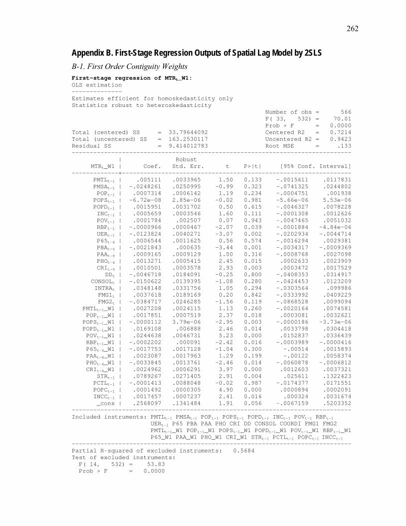
262
Appendix B. First-Stage Regression Outputs of Spatial Lag Model by 2SLS B-1. First Order Contiguity Weights First-stage regression of MTRt_W1: OLS estimation -------------- Estimates efficient for homoskedasticity only Statistics robust to heteroskedasticity Number of obs = 566 F( 33, 532) = 70.01 Prob > F = 0.0000 Total (centered) SS = 33.79644092 Centered R2 = 0.7214 Total (uncentered) SS = 163.2530117 Uncentered R2 = 0.9423 Residual SS = 9.414012783 Root MSE = .133 ------------------------------------------------------------------------------ | Robust MTRt_W1 | Coef. Std. Err. t P>|t| [95% Conf. Interval] -------------+---------------------------------------------------------------- PMTLt-1 | .005111 .0033965 1.50 0.133 -.0015611 .0117831 PMSAt-1 | -.0248261 .0250995 -0.99 0.323 -.0741325 .0244802 POPt-1 | .0007314 .0006142 1.19 0.234 -.0004751 .001938 POPSt-1 | -6.72e-08 2.85e-06 -0.02 0.981 -5.66e-06 5.53e-06 POPDt-1 | .0015951 .0031702 0.50 0.615 -.0046327 .0078228 INCt-1 | .0005659 .0003546 1.60 0.111 -.0001308 .0012626 POVt-1 | .0001784 .002507 0.07 0.943 -.0047465 .0051032 RBPt-1 | -.0000966 .0000467 -2.07 0.039 -.0001884 -4.84e-06 UERt-1 | -.0123824 .0040271 -3.07 0.002 -.0202934 -.0044714 P65t-4 | .0006544 .0011625 0.56 0.574 -.0016294 .0029381 PBAt-4 | -.0021843 .000635 -3.44 0.001 -.0034317 -.0009369 PAAt-4 | .0009165 .0009129 1.00 0.316 -.0008768 .0027098 PHOt-4 | .0013271 .0005415 2.45 0.015 .0002633 .0023909 CRIt-4 | .0010501 .0003578 2.93 0.003 .0003472 .0017529 DDt | -.0046718 .0184091 -0.25 0.800 -.0408353 .0314917 CONSOLt | -.0150622 .0139395 -1.08 0.280 -.0424453 .0123209 INTRAt | .0348148 .0331756 1.05 0.294 -.0303564 .099986 FMG1t | .0037618 .0189169 0.20 0.842 -.0333992 .0409229 FMG2t | -.0384717 .0246285 -1.56 0.119 -.0868528 .0099094 PMTLt-1_W1 | .0027208 .0024115 1.13 0.260 -.0020164 .0074581 POPt-1_W1 | .0017851 .0007519 2.37 0.018 .0003081 .0032621 POPSt-1_W1 | -.0000112 3.79e-06 -2.95 0.003 -.0000186 -3.73e-06 POPDt-1_W1 | .0169108 .006888 2.46 0.014 .0033798 .0304418 POVt-1_W1 | .0244638 .0046731 5.23 0.000 .0152837 .0336439 RBPt-1_W1 | -.0002202 .000091 -2.42 0.016 -.0003989 -.0000416 P65t-4_W1 | -.0017753 .0017128 -1.04 0.300 -.00514 .0015893 PAAt-4_W1 | .0023087 .0017963 1.29 0.199 -.00122 .0058374 PHOt-4_W1 | -.0033845 .0013761 -2.46 0.014 -.0060878 -.0006812 CRIt-4_W1 | .0024962 .0006291 3.97 0.000 .0012603 .0037321 STRt-1 | .0789267 .0271405 2.91 0.004 .025611 .1322423 PCTLt-1 | -.0001413 .0088048 -0.02 0.987 -.0174377 .0171551 POPCt-1 | .0001492 .0000305 4.90 0.000 .0000894 .0002091 INCCt-1 | .0017457 .0007237 2.41 0.016 .000324 .0031674 _cons | .2568097 .1341484 1.91 0.056 -.0067159 .5203352 ------------------------------------------------------------------------------ Included instruments: PMTLt-1 PMSAt-1 POPt-1 POPSt-1 POPDt-1 INCt-1 POVt-1 RBPt-1 UERt-1 P65 PBA PAA PHO CRI DD CONSOL COORDI FMG1 FMG2 PMTLt-1_W1 POPt-1_W1 POPSt-1_W1 POPDt-1_W1 POVt-1_W1 RBPt-1_W1 P65_W1 PAA_W1 PHO_W1 CRI_W1 STRt-1 PCTLt-1 POPCt-1 INCCt-1 ------------------------------------------------------------------------------ Partial R-squared of excluded instruments: 0.5684 Test of excluded instruments: F( 14, 532) = 53.83 Prob > F = 0.0000

263
First-stage regression of STRt: OLS estimation -------------- Estimates efficient for homoskedasticity only Statistics robust to heteroskedasticity Number of obs = 566 F( 33, 532) = 230.81 Prob > F = 0.0000 Total (centered) SS = 168.7782268 Centered R2 = 0.9050 Total (uncentered) SS = 990.6832035 Uncentered R2 = 0.9838 Residual SS = 16.03158899 Root MSE = .1736 ------------------------------------------------------------------------------ | Robust STRt | Coef. Std. Err. t P>|t| [95% Conf. Interval] -------------+---------------------------------------------------------------- PMTLt-1 | .002843 .0057138 0.50 0.619 -.0083815 .0140675 PMSAt-1 | .0065882 .0304132 0.22 0.829 -.0531565 .0663329 POPt-1 | -.0003008 .0005561 -0.54 0.589 -.0013931 .0007916 POPSt-1 | 1.03e-06 2.53e-06 0.41 0.683 -3.94e-06 6.01e-06 POPDt-1 | -.0044264 .0033481 -1.32 0.187 -.0110034 .0021507 INCt-1 | .0042603 .0030105 1.42 0.158 -.0016536 .0101743 POVt-1 | .0024537 .0022329 1.10 0.272 -.0019327 .0068401 RBPt-1 | -2.61e-06 .0000413 -0.06 0.950 -.0000837 .0000785 UERt-1 | -.0042301 .005403 -0.78 0.434 -.014844 .0063838 P65t-4 | .0005078 .001999 0.25 0.800 -.003419 .0044346 PBAt-4 | -.0029294 .0030688 -0.95 0.340 -.008958 .0030991 PAAt-4 | -.000855 .0010363 -0.83 0.410 -.0028909 .0011808 PHOt-4 | .0003108 .0006873 0.45 0.651 -.0010394 .0016609 CRIt-4 | .0002937 .0004054 0.72 0.469 -.0005027 .00109 DDt | .0374115 .0372905 1.00 0.316 -.0358432 .1106661 CONSOLt | .018476 .0139404 1.33 0.186 -.0089091 .045861 INTRAt | -.262779 .1778689 -1.48 0.140 -.6121906 .0866326 FMG1t | .0218924 .0173265 1.26 0.207 -.0121443 .0559291 FMG2t | .0323977 .0268678 1.21 0.228 -.0203823 .0851778 PMTLt-1_W1 | .0027572 .001614 1.71 0.088 -.0004134 .0059278 POPt-1_W1 | .0002332 .000825 0.28 0.778 -.0013875 .001854 POPSt-1_W1 | -5.49e-06 4.64e-06 -1.18 0.237 -.0000146 3.62e-06 POPDt-1_W1 | .0085499 .0053099 1.61 0.108 -.0018811 .0189809 POVt-1_W1 | -.0023869 .0075229 -0.32 0.751 -.0171652 .0123913 RBPt-1_W1 | -.0000913 .0001195 -0.76 0.445 -.000326 .0001433 P65t-4_W1 | .0048016 .0042748 1.12 0.262 -.003596 .0131991 PAAt-4_W1 | .0057353 .0049709 1.15 0.249 -.0040297 .0155002 PHOt-4_W1 | .0001209 .0008587 0.14 0.888 -.001566 .0018077 CRIt-4_W1 | -.0012692 .0008143 -1.56 0.120 -.0028687 .0003304 STRt-1 | 1.060595 .033257 31.89 0.000 .9952639 1.125926 PCTLt-1 | -.0054257 .0144163 -0.38 0.707 -.0337456 .0228943 POPCt-1 | -.0000589 .0000308 -1.91 0.056 -.0001194 1.55e-06 INCCt-1 | .0017099 .0007773 2.20 0.028 .0001831 .0032368 _cons | -.1184549 .1905237 -0.62 0.534 -.492726 .2558162 ------------------------------------------------------------------------------ Included instruments: PMTLt-1 PMSAt-1 POPt-1 POPSt-1 POPDt-1 INCt-1 POVt-1 RBPt-1 UERt-1 P65 PBA PAA PHO CRI DD CONSOL COORDI FMG1 FMG2 PMTLt-1_W1 POPt-1_W1 POPSt-1_W1 POPDt-1_W1 POVt-1_W1 RBPt-1_W1 P65_W1 PAA_W1 PHO_W1 CRI_W1 STRt-1 PCTLt-1 POPCt-1 INCCt-1 ------------------------------------------------------------------------------ Partial R-squared of excluded instruments: 0.8708 Test of excluded instruments: F( 14, 532) = 123.14 Prob > F = 0.0000

264
First-stage regression of CTRt: OLS estimation -------------- Estimates efficient for homoskedasticity only Statistics robust to heteroskedasticity Number of obs = 566 F( 33, 532) = 55.30 Prob > F = 0.0000 Total (centered) SS = 21.38244407 Centered R2 = 0.7279 Total (uncentered) SS = 124.4604994 Uncentered R2 = 0.9532 Residual SS = 5.81892598 Root MSE = .1046 ------------------------------------------------------------------------------ | Robust CTRt | Coef. Std. Err. t P>|t| [95% Conf. Interval] -------------+---------------------------------------------------------------- PMTLt-1 | -.0076074 .0031858 -2.39 0.017 -.0138657 -.0013492 PMSAt-1 | .0392653 .0223669 1.76 0.080 -.0046729 .0832035 POPt-1 | .0006966 .0003883 1.79 0.073 -.0000663 .0014595 POPSt-1 | -2.20e-06 1.69e-06 -1.30 0.193 -5.51e-06 1.11e-06 POPDt-1 | .0009984 .0011008 0.91 0.365 -.001164 .0031608 INCt-1 | .0006005 .0003204 1.87 0.061 -.000029 .00123 POVt-1 | .0062372 .0021408 2.91 0.004 .0020316 .0104427 RBPt-1 | -.0000699 .000043 -1.63 0.104 -.0001543 .0000145 UERt-1 | -.0117366 .0033416 -3.51 0.000 -.018301 -.0051721 P65t-4 | -.0001416 .0010592 -0.13 0.894 -.0022223 .0019391 PBAt-4 | -.0001524 .0005278 -0.29 0.773 -.0011892 .0008844 PAAt-4 | .0011377 .0007811 1.46 0.146 -.0003967 .0026722 PHOt-4 | .0000378 .0005717 0.07 0.947 -.0010852 .0011609 CRIt-4 | -.0004433 .0003864 -1.15 0.252 -.0012022 .0003157 DDt | -.009674 .0115321 -0.84 0.402 -.0323281 .0129801 CONSOLt | -.0107389 .0140514 -0.76 0.445 -.0383419 .0168641 INTRAt | .0151906 .0258371 0.59 0.557 -.0355647 .0659458 FMG1t | .0399406 .0154547 2.58 0.010 .0095809 .0703003 FMG2t | .0321839 .0183117 1.76 0.079 -.0037882 .068156 PMTLt-1_W1 | -.0021622 .0011753 -1.84 0.066 -.004471 .0001465 POPt-1_W1 | -.0009095 .0005595 -1.63 0.105 -.0020086 .0001896 POPSt-1_W1 | 1.11e-06 2.89e-06 0.39 0.700 -4.57e-06 6.79e-06 POPDt-1_W1 | .0010314 .0018581 0.56 0.579 -.0026186 .0046815 POVt-1_W1 | .0192929 .0043691 4.42 0.000 .0107101 .0278756 RBPt-1_W1 | -.0002431 .0000736 -3.31 0.001 -.0003876 -.0000986 P65t-4_W1 | -.0005918 .001099 -0.54 0.590 -.0027508 .0015672 PAAt-4_W1 | .0013526 .0013579 1.00 0.320 -.0013149 .00402 PHOt-4_W1 | -.0010818 .00081 -1.34 0.182 -.0026731 .0005094 CRIt-4_W1 | -.0033093 .0005451 -6.07 0.000 -.0043801 -.0022386 STRt-1 | .0692904 .0271578 2.55 0.011 .0159408 .12264 PCTLt-1 | .0180529 .008963 2.01 0.044 .0004458 .03566 POPCt-1 | -.0002652 .0000233 -11.40 0.000 -.0003109 -.0002195 INCCt-1 | -.0111715 .0005836 -19.14 0.000 -.012318 -.0100249 _cons | 1.03874 .1137532 9.13 0.000 .8152798 1.262201 ------------------------------------------------------------------------------ Included instruments: PMTLt-1 PMSAt-1 POPt-1 POPSt-1 POPDt-1 INCt-1 POVt-1 RBPt-1 UERt-1 P65 PBA PAA PHO CRI DD CONSOL COORDI FMG1 FMG2 PMTLt-1_W1 POPt-1_W1 POPSt-1_W1 POPDt-1_W1 POVt-1_W1 RBPt-1_W1 P65_W1 PAA_W1 PHO_W1 CRI_W1 STRt-1 PCTLt-1 POPCt-1 INCCt-1 ------------------------------------------------------------------------------ Partial R-squared of excluded instruments: 0.5953 Test of excluded instruments: F( 14, 532) = 68.62 Prob > F = 0.0000

265
B-2. Second Order Contiguity Weights
First-stage regression of MTRt_W2: OLS estimation -------------- Estimates efficient for homoskedasticity only Statistics robust to heteroskedasticity Number of obs = 566 F( 33, 532) = 69.66 Prob > F = 0.0000 Total (centered) SS = 24.40258876 Centered R2 = 0.7364 Total (uncentered) SS = 157.1858406 Uncentered R2 = 0.9591 Residual SS = 6.432464979 Root MSE = .11 ------------------------------------------------------------------------------ | Robust MTRt_W2 | Coef. Std. Err. t P>|t| [95% Conf. Interval] -------------+---------------------------------------------------------------- PMTLt-1 | .0020679 .0023582 0.88 0.381 -.0025647 .0067005 PMSAt-1 | -.003363 .0179736 -0.19 0.852 -.0386709 .031945 POPt-1 | .0014242 .0005515 2.58 0.010 .0003409 .0025076 POPSt-1 | -4.99e-06 2.21e-06 -2.26 0.024 -9.33e-06 -6.47e-07 POPDt-1 | .0009598 .0015893 0.60 0.546 -.0021623 .0040818 INCt-1 | .0005363 .0002662 2.01 0.044 .0000133 .0010592 POVt-1 | -.0001805 .0021393 -0.08 0.933 -.0043829 .004022 RBPt-1 | -.0000279 .0000541 -0.52 0.606 -.0001343 .0000784 UERt-1 | -.0031593 .003082 -1.03 0.306 -.0092136 .002895 P65t-4 | .0000526 .0010492 0.05 0.960 -.0020085 .0021138 PBAt-4 | -.0003823 .0005106 -0.75 0.454 -.0013854 .0006207 PAAt-4 | .0001846 .0006508 0.28 0.777 -.0010939 .0014632 PHOt-4 | .0007207 .0003975 1.81 0.070 -.0000602 .0015016 CRIt-4 | .0005374 .0002085 2.58 0.010 .0001279 .0009469 DDt | -.011399 .0143095 -0.80 0.426 -.039509 .016711 CONSOLt | -.0182272 .0113973 -1.60 0.110 -.0406164 .0041619 INTRAt | -.0526527 .0259885 -2.03 0.043 -.1037053 -.0016001 FMG1t | .0135338 .0175875 0.77 0.442 -.0210156 .0480833 FMG2t | -.0125221 .0209594 -0.60 0.550 -.0536955 .0286513 PMTLt-1_W2 | -.0011614 .0039892 -0.29 0.771 -.0089979 .006675 POPt-1_W2 | .0073957 .0013586 5.44 0.000 .0047268 .0100645 POPSt-1_W2 | -.000038 8.44e-06 -4.51 0.000 -.0000546 -.0000214 POPDt-1_W2 | .025185 .005046 4.99 0.000 .0152725 .0350975 POVt-1_W2 | .0366784 .0048018 7.64 0.000 .0272457 .0461112 RBPt-1_W2 | -.0007424 .000139 -5.34 0.000 -.0010155 -.0004694 P65t-4_W2 | -.0095355 .0029009 -3.29 0.001 -.0152342 -.0038367 PAAt-4_W2 | -.0238931 .0083688 -2.86 0.004 -.040333 -.0074532 PHOt-4_W2 | -.0018625 .001441 -1.29 0.197 -.0046932 .0009682 CRIt-4_W2 | .0040217 .0008824 4.56 0.000 .0022883 .0057552 STRt-1 | .0670488 .0206689 3.24 0.001 .0264461 .1076515 PCTLt-1 | -.0045571 .0072942 -0.62 0.532 -.0188861 .0097718 POPCt-1 | .0000708 .0000284 2.50 0.013 .0000151 .0001264 INCCt-1 | .0003777 .0006004 0.63 0.530 -.0008017 .0015571 _cons | .3070403 .1302701 2.36 0.019 .0511334 .5629473 ------------------------------------------------------------------------------ Included instruments: PMTLt-1 PMSAt-1 POPt-1 POPSt-1 POPDt-1 INCt-1 POVt-1 RBPt-1 UERt-1 P65 PBA PAA PHO CRI DD CONSOL COORDI FMG1 FMG2 PMTLt-1_W2 POPt-1_W2 POPSt-1_W2 POPDt-1_W2 POVt-1_W2 RBPt-1_W2 P65_W2 PAA_W2 PHO_W2 CRI_W2 STRt-1 PCTLt-1 POPCt-1 INCCt-1 ------------------------------------------------------------------------------ Partial R-squared of excluded instruments: 0.6235 Test of excluded instruments: F( 14, 532) = 58.19 Prob > F = 0.0000

266
First-stage regression of STRt: OLS estimation -------------- Estimates efficient for homoskedasticity only Statistics robust to heteroskedasticity Number of obs = 566 F( 33, 532) = 414.48 Prob > F = 0.0000 Total (centered) SS = 168.7782268 Centered R2 = 0.9036 Total (uncentered) SS = 990.6832035 Uncentered R2 = 0.9836 Residual SS = 16.26775596 Root MSE = .1749 ------------------------------------------------------------------------------ | Robust STRt | Coef. Std. Err. t P>|t| [95% Conf. Interval] -------------+---------------------------------------------------------------- PMTLt-1 | .00109 .0053348 0.20 0.838 -.0093899 .0115699 PMSAt-1 | .011603 .0279062 0.42 0.678 -.0432169 .066423 POPt-1 | -.000344 .0006079 -0.57 0.572 -.0015382 .0008501 POPSt-1 | 3.49e-07 2.79e-06 0.13 0.900 -5.13e-06 5.83e-06 POPDt-1 | -.0032543 .002957 -1.10 0.272 -.009063 .0025545 INCt-1 | .0044874 .0032994 1.36 0.174 -.001994 .0109688 POVt-1 | .0026594 .0020641 1.29 0.198 -.0013954 .0067143 RBPt-1 | -.0000262 .0000453 -0.58 0.563 -.0001152 .0000627 UERt-1 | -.0086409 .0081395 -1.06 0.289 -.0246304 .0073485 P65t-4 | -.0000555 .0021393 -0.03 0.979 -.004258 .004147 PBAt-4 | -.0033546 .0033027 -1.02 0.310 -.0098426 .0031334 PAAt-4 | .0002738 .0007284 0.38 0.707 -.0011572 .0017047 PHOt-4 | .000636 .0006519 0.98 0.330 -.0006447 .0019167 CRIt-4 | .0003111 .0003982 0.78 0.435 -.0004712 .0010933 DDt | .0470051 .0442579 1.06 0.289 -.0399367 .1339469 CONSOLt | .0239211 .0144445 1.66 0.098 -.0044542 .0522964 INTRAt | -.242349 .1711032 -1.42 0.157 -.5784698 .0937718 FMG1t | .0322649 .021727 1.49 0.138 -.0104165 .0749462 FMG2t | .0461797 .0326924 1.41 0.158 -.0180424 .1104018 PMTLt-1_W2 | -.0012543 .0046844 -0.27 0.789 -.0104566 .0079479 POPt-1_W2 | -.0001571 .0011506 -0.14 0.891 -.0024175 .0021032 POPSt-1_W2 | -6.20e-06 8.70e-06 -0.71 0.477 -.0000233 .0000109 POPDt-1_W2 | .0163739 .0063293 2.59 0.010 .0039404 .0288073 POVt-1_W2 | -.0102206 .0074109 -1.38 0.168 -.0247788 .0043376 RBPt-1_W2 | -.0000732 .0001717 -0.43 0.670 -.0004106 .0002641 P65t-4_W2 | .0086015 .0066292 1.30 0.195 -.0044212 .0216242 PAAt-4_W2 | .0115221 .0101612 1.13 0.257 -.0084389 .031483 PHOt-4_W2 | 7.57e-07 .0015994 0.00 1.000 -.0031411 .0031426 CRIt-4_W2 | -.0000691 .000831 -0.08 0.934 -.0017015 .0015632 STRt-1 | 1.079154 .0408135 26.44 0.000 .9989783 1.159329 PCTLt-1 | -.0014508 .0143855 -0.10 0.920 -.0297102 .0268086 POPCt-1 | -.0000888 .0000389 -2.28 0.023 -.0001652 -.0000125 INCCt-1 | .0011848 .0008174 1.45 0.148 -.000421 .0027906 _cons | -.1795095 .2514506 -0.71 0.476 -.6734673 .3144484 ------------------------------------------------------------------------------ Included instruments: PMTLt-1 PMSAt-1 POPt-1 POPSt-1 POPDt-1 INCt-1 POVt-1 RBPt-1 UERt-1 P65 PBA PAA PHO CRI DD CONSOL COORDI FMG1 FMG2 PMTLt-1_W2 POPt-1_W2 POPSt-1_W2 POPDt-1_W2 POVt-1_W2 RBPt-1_W2 P65_W2 PAA_W2 PHO_W2 CRI_W2 STRt-1 PCTLt-1 POPCt-1 INCCt-1 ------------------------------------------------------------------------------ Partial R-squared of excluded instruments: 0.8689 Test of excluded instruments: F( 14, 532) = 192.89 Prob > F = 0.0000
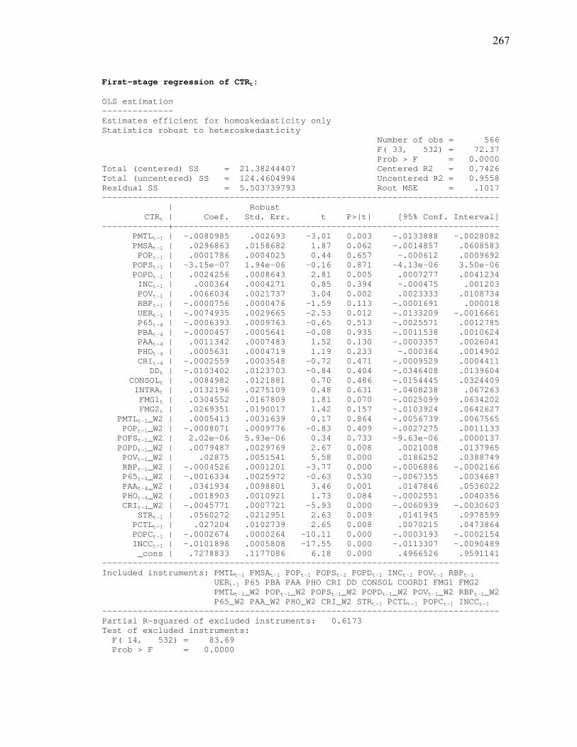
267
First-stage regression of CTRt: OLS estimation -------------- Estimates efficient for homoskedasticity only Statistics robust to heteroskedasticity Number of obs = 566 F( 33, 532) = 72.37 Prob > F = 0.0000 Total (centered) SS = 21.38244407 Centered R2 = 0.7426 Total (uncentered) SS = 124.4604994 Uncentered R2 = 0.9558 Residual SS = 5.503739793 Root MSE = .1017 ------------------------------------------------------------------------------ | Robust CTRt | Coef. Std. Err. t P>|t| [95% Conf. Interval] -------------+---------------------------------------------------------------- PMTLt-1 | -.0080985 .002693 -3.01 0.003 -.0133888 -.0028082 PMSAt-1 | .0296863 .0158682 1.87 0.062 -.0014857 .0608583 POPt-1 | .0001786 .0004025 0.44 0.657 -.000612 .0009692 POPSt-1 | -3.15e-07 1.94e-06 -0.16 0.871 -4.13e-06 3.50e-06 POPDt-1 | .0024256 .0008643 2.81 0.005 .0007277 .0041234 INCt-1 | .000364 .0004271 0.85 0.394 -.000475 .001203 POVt-1 | .0066034 .0021737 3.04 0.002 .0023333 .0108734 RBPt-1 | -.0000756 .0000476 -1.59 0.113 -.0001691 .000018 UERt-1 | -.0074935 .0029665 -2.53 0.012 -.0133209 -.0016661 P65t-4 | -.0006393 .0009763 -0.65 0.513 -.0025571 .0012785 PBAt-4 | -.0000457 .0005641 -0.08 0.935 -.0011538 .0010624 PAAt-4 | .0011342 .0007483 1.52 0.130 -.0003357 .0026041 PHOt-4 | .0005631 .0004719 1.19 0.233 -.000364 .0014902 CRIt-4 | -.0002559 .0003548 -0.72 0.471 -.0009529 .0004411 DDt | -.0103402 .0123703 -0.84 0.404 -.0346408 .0139604 CONSOLt | .0084982 .0121881 0.70 0.486 -.0154445 .0324409 INTRAt | .0132196 .0275109 0.48 0.631 -.0408238 .067263 FMG1t | .0304552 .0167809 1.81 0.070 -.0025099 .0634202 FMG2t | .0269351 .0190017 1.42 0.157 -.0103924 .0642627 PMTLt-1_W2 | .0005413 .0031639 0.17 0.864 -.0056739 .0067565 POPt-1_W2 | -.0008071 .0009776 -0.83 0.409 -.0027275 .0011133 POPSt-1_W2 | 2.02e-06 5.93e-06 0.34 0.733 -9.63e-06 .0000137 POPDt-1_W2 | .0079487 .0029769 2.67 0.008 .0021008 .0137965 POVt-1_W2 | .02875 .0051541 5.58 0.000 .0186252 .0388749 RBPt-1_W2 | -.0004526 .0001201 -3.77 0.000 -.0006886 -.0002166 P65t-4_W2 | -.0016334 .0025972 -0.63 0.530 -.0067355 .0034687 PAAt-4_W2 | .0341934 .0098801 3.46 0.001 .0147846 .0536022 PHOt-4_W2 | .0018903 .0010921 1.73 0.084 -.0002551 .0040356 CRIt-4_W2 | -.0045771 .0007721 -5.93 0.000 -.0060939 -.0030603 STRt-1 | .0560272 .0212951 2.63 0.009 .0141945 .0978599 PCTLt-1 | .027204 .0102739 2.65 0.008 .0070215 .0473864 POPCt-1 | -.0002674 .0000264 -10.11 0.000 -.0003193 -.0002154 INCCt-1 | -.0101898 .0005808 -17.55 0.000 -.0113307 -.0090489 _cons | .7278833 .1177086 6.18 0.000 .4966526 .9591141 ------------------------------------------------------------------------------ Included instruments: PMTLt-1 PMSAt-1 POPt-1 POPSt-1 POPDt-1 INCt-1 POVt-1 RBPt-1 UERt-1 P65 PBA PAA PHO CRI DD CONSOL COORDI FMG1 FMG2 PMTLt-1_W2 POPt-1_W2 POPSt-1_W2 POPDt-1_W2 POVt-1_W2 RBPt-1_W2 P65_W2 PAA_W2 PHO_W2 CRI_W2 STRt-1 PCTLt-1 POPCt-1 INCCt-1 ------------------------------------------------------------------------------ Partial R-squared of excluded instruments: 0.6173 Test of excluded instruments: F( 14, 532) = 83.69 Prob > F = 0.0000

268
B-3. Distance Weights
First-stage regression of MTRt_W3: OLS estimation -------------- Estimates efficient for homoskedasticity only Statistics robust to heteroskedasticity Number of obs = 566 F( 33, 532) = 61.28 Prob > F = 0.0000 Total (centered) SS = 25.98162379 Centered R2 = 0.7332 Total (uncentered) SS = 178.6132341 Uncentered R2 = 0.9612 Residual SS = 6.932105851 Root MSE = .1142 ------------------------------------------------------------------------------ | Robust MTRt_W3 | Coef. Std. Err. t P>|t| [95% Conf. Interval] -------------+---------------------------------------------------------------- PMTLt-1 | -.0000449 .0034157 -0.01 0.990 -.0067548 .0066651 PMSAt-1 | .004427 .0239215 0.19 0.853 -.0425653 .0514192 POPt-1 | .0008828 .0006363 1.39 0.166 -.0003672 .0021328 POPSt-1 | -2.09e-06 3.19e-06 -0.66 0.512 -8.37e-06 4.18e-06 POPDt-1 | .001869 .0012551 1.49 0.137 -.0005965 .0043346 INCt-1 | .0008564 .0003271 2.62 0.009 .0002137 .001499 POVt-1 | -.0003243 .0021957 -0.15 0.883 -.0046376 .0039891 RBPt-1 | -.0000677 .0000614 -1.10 0.271 -.0001884 .000053 UERt-1 | -.0083898 .0031812 -2.64 0.009 -.0146391 -.0021405 P65t-4 | .0001725 .0013065 0.13 0.895 -.002394 .002739 PBAt-4 | -.0020937 .0005429 -3.86 0.000 -.0031603 -.0010272 PAAt-4 | .0005061 .0007238 0.70 0.485 -.0009158 .0019279 PHOt-4 | .001762 .0004845 3.64 0.000 .0008102 .0027138 CRIt-4 | .0009308 .0002861 3.25 0.001 .0003688 .0014928 DDt | -.0027037 .0137522 -0.20 0.844 -.0297191 .0243116 CONSOLt | .0009228 .0127939 0.07 0.943 -.02421 .0260557 INTRAt | -.0549128 .0347388 -1.58 0.115 -.1231548 .0133292 FMG1t | -.0053769 .0176509 -0.30 0.761 -.0400509 .0292971 FMG2t | -.041084 .0215001 -1.91 0.057 -.0833195 .0011516 PMTLt-1_W3 | -.0197832 .0090401 -2.19 0.029 -.0375418 -.0020246 POPt-1_W3 | .0078838 .0013973 5.64 0.000 .005139 .0106286 POPSt-1_W3 | -.0000478 8.68e-06 -5.51 0.000 -.0000648 -.0000307 POPDt-1_W3 | .0522957 .006335 8.26 0.000 .0398511 .0647403 POVt-1_W3 | .0205622 .0058566 3.51 0.000 .0090573 .0320671 RBPt-1_W3 | -.0007622 .0001886 -4.04 0.000 -.0011326 -.0003917 P65t-4_W3 | -.0044173 .0023044 -1.92 0.056 -.0089441 .0001094 PAAt-4_W3 | .0038456 .0021132 1.82 0.069 -.0003055 .0079968 PHOt-4_W3 | .0031505 .0015571 2.02 0.044 .0000916 .0062093 CRIt-4_W3 | .0046629 .0009361 4.98 0.000 .0028241 .0065017 STRt-1 | .0787726 .0301693 2.61 0.009 .019507 .1380381 PCTLt-1 | .0014652 .009787 0.15 0.881 -.0177608 .0206912 POPCt-1 | -.0000488 .0000309 -1.58 0.115 -.0001096 .000012 INCCt-1 | .0008829 .0006694 1.32 0.188 -.000432 .0021979 _cons | -.197774 .1500299 -1.32 0.188 -.4924978 .0969498 ------------------------------------------------------------------------------ Included instruments: PMTLt-1 PMSAt-1 POPt-1 POPSt-1 POPDt-1 INCt-1 POVt-1 RBPt-1 UERt-1 P65 PBA PAA PHO CRI DD CONSOL COORDI FMG1 FMG2 PMTLt-1_W3 POPt-1_W3 POPSt-1_W3 POPDt-1_W3 POVt-1_W3 RBPt-1_W3 P65_W3 PAA_W3 PHO_W3 CRI_W3 STRt-1 PCTLt-1 POPCt-1 INCCt-1 ------------------------------------------------------------------------------ Partial R-squared of excluded instruments: 0.6232 Test of excluded instruments: F( 14, 532) = 62.14 Prob > F = 0.0000

269
First-stage regression of STRt: OLS estimation -------------- Estimates efficient for homoskedasticity only Statistics robust to heteroskedasticity Number of obs = 566 F( 33, 532) = 335.90 Prob > F = 0.0000 Total (centered) SS = 168.7782268 Centered R2 = 0.9039 Total (uncentered) SS = 990.6832035 Uncentered R2 = 0.9836 Residual SS = 16.21786763 Root MSE = .1746 ------------------------------------------------------------------------------ | Robust STRt | Coef. Std. Err. t P>|t| [95% Conf. Interval] -------------+---------------------------------------------------------------- PMTLt-1 | .0010187 .0051529 0.20 0.843 -.0091039 .0111413 PMSAt-1 | .0208021 .024839 0.84 0.403 -.0279924 .0695966 POPt-1 | -.0005472 .0006154 -0.89 0.374 -.0017561 .0006616 POPSt-1 | 1.63e-06 2.80e-06 0.58 0.560 -3.86e-06 7.13e-06 POPDt-1 | -.0043095 .0035701 -1.21 0.228 -.0113228 .0027037 INCt-1 | .0045056 .0032743 1.38 0.169 -.0019266 .0109377 POVt-1 | .0030196 .0021792 1.39 0.166 -.0012613 .0073005 RBPt-1 | -.0000183 .0000379 -0.48 0.629 -.0000928 .0000562 UERt-1 | -.0074889 .0079 -0.95 0.344 -.0230079 .0080301 P65t-4 | -.00004 .0022365 -0.02 0.986 -.0044336 .0043535 PBAt-4 | -.0031307 .0031856 -0.98 0.326 -.0093885 .0031271 PAAt-4 | .0005454 .0008119 0.67 0.502 -.0010496 .0021404 PHOt-4 | .0007007 .0006481 1.08 0.280 -.0005725 .0019738 CRIt-4 | .0001875 .0004008 0.47 0.640 -.0005999 .000975 DDt | .0487946 .0427513 1.14 0.254 -.0351875 .1327767 CONSOLt | .0304159 .0173112 1.76 0.079 -.0035908 .0644225 INTRAt | -.27061 .1865732 -1.45 0.148 -.6371205 .0959006 FMG1t | .0274712 .0211935 1.30 0.195 -.0141621 .0691044 FMG2t | .0474649 .0343554 1.38 0.168 -.020024 .1149538 PMTLt-1_W3 | .0023579 .0070961 0.33 0.740 -.011582 .0162978 POPt-1_W3 | .0027458 .0017572 1.56 0.119 -.000706 .0061976 POPSt-1_W3 | -.0000361 .0000185 -1.95 0.051 -.0000724 2.33e-07 POPDt-1_W3 | .0190578 .0071305 2.67 0.008 .0050504 .0330651 POVt-1_W3 | -.000394 .0059194 -0.07 0.947 -.0120224 .0112343 RBPt-1_W3 | -.0000533 .0002256 -0.24 0.813 -.0004965 .0003899 P65t-4_W3 | .0029078 .0022565 1.29 0.198 -.001525 .0073406 PAAt-4_W3 | -.0010025 .0032185 -0.31 0.756 -.007325 .0053201 PHOt-4_W3 | .0004297 .0013189 0.33 0.745 -.0021613 .0030206 CRIt-4_W3 | .0002477 .0009419 0.26 0.793 -.0016025 .0020979 STRt-1 | 1.076709 .0403488 26.69 0.000 .9974466 1.155972 PCTLt-1 | -.0066006 .0158504 -0.42 0.677 -.0377376 .0245365 POPCt-1 | -.0001003 .0000323 -3.11 0.002 -.0001637 -.0000369 INCCt-1 | .0008651 .0007991 1.08 0.279 -.0007046 .0024348 _cons | -.1534489 .2499334 -0.61 0.540 -.6444263 .3375285 ------------------------------------------------------------------------------ Included instruments: PMTLt-1 PMSAt-1 POPt-1 POPSt-1 POPDt-1 INCt-1 POVt-1 RBPt-1 UERt-1 P65 PBA PAA PHO CRI DD CONSOL COORDI FMG1 FMG2 PMTLt-1_W3 POPt-1_W3 POPSt-1_W3 POPDt-1_W3 POVt-1_W3 RBPt-1_W3 P65_W3 PAA_W3 PHO_W3 CRI_W3 STRt-1 PCTLt-1 POPCt-1 INCCt-1 ------------------------------------------------------------------------------ Partial R-squared of excluded instruments: 0.8693 Test of excluded instruments: F( 14, 532) = 175.43 Prob > F = 0.0000

270
First-stage regression of CTRt: OLS estimation -------------- Estimates efficient for homoskedasticity only Statistics robust to heteroskedasticity Number of obs = 566 F( 33, 532) = 55.72 Prob > F = 0.0000 Total (centered) SS = 21.38244407 Centered R2 = 0.7335 Total (uncentered) SS = 124.4604994 Uncentered R2 = 0.9542 Residual SS = 5.699320441 Root MSE = .1035 ------------------------------------------------------------------------------ | Robust CTRt | Coef. Std. Err. t P>|t| [95% Conf. Interval] -------------+---------------------------------------------------------------- PMTLt-1 | -.0085176 .0036092 -2.36 0.019 -.0156077 -.0014275 PMSAt-1 | .0253244 .0258978 0.98 0.329 -.02555 .0761988 POPt-1 | .000295 .0004063 0.73 0.468 -.0005032 .0010931 POPSt-1 | -1.88e-06 1.87e-06 -1.01 0.315 -5.55e-06 1.79e-06 POPDt-1 | .0018593 .000912 2.04 0.042 .0000677 .0036508 INCt-1 | .0003841 .0003698 1.04 0.299 -.0003424 .0011105 POVt-1 | .0075658 .0019867 3.81 0.000 .0036631 .0114685 RBPt-1 | -.0000495 .0000529 -0.93 0.350 -.0001534 .0000545 UERt-1 | -.008743 .0031103 -2.81 0.005 -.014853 -.0026331 P65t-4 | -.00105 .0010484 -1.00 0.317 -.0031096 .0010096 PBAt-4 | .000197 .0005372 0.37 0.714 -.0008584 .0012523 PAAt-4 | .0007672 .0007553 1.02 0.310 -.0007166 .002251 PHOt-4 | .0003978 .0005037 0.79 0.430 -.0005918 .0013874 CRIt-4 | -.0003265 .0004048 -0.81 0.420 -.0011217 .0004686 DDt | -.0071503 .0120831 -0.59 0.554 -.0308868 .0165862 CONSOLt | .0065781 .0132613 0.50 0.620 -.0194728 .032629 INTRAt | .0111952 .0291162 0.38 0.701 -.0460016 .068392 FMG1t | .0373968 .0160371 2.33 0.020 .0058929 .0689007 FMG2t | .0325232 .0182285 1.78 0.075 -.0032855 .0683319 PMTLt-1_W3 | -.0053057 .0072049 -0.74 0.462 -.0194592 .0088478 POPt-1_W3 | -.0008782 .001125 -0.78 0.435 -.0030883 .0013318 POPSt-1_W3 | -7.71e-07 7.52e-06 -0.10 0.918 -.0000155 .000014 POPDt-1_W3 | .0201418 .0046677 4.32 0.000 .0109725 .0293112 POVt-1_W3 | .0204792 .004396 4.66 0.000 .0118437 .0291148 RBPt-1_W3 | -.0005105 .000149 -3.43 0.001 -.0008032 -.0002178 P65t-4_W3 | -.0019897 .001516 -1.31 0.190 -.0049678 .0009885 PAAt-4_W3 | .0041163 .0016668 2.47 0.014 .000842 .0073905 PHOt-4_W3 | .0032331 .0012189 2.65 0.008 .0008387 .0056276 CRIt-4_W3 | -.0030691 .0007218 -4.25 0.000 -.0044871 -.0016512 STRt-1 | .0578928 .0224668 2.58 0.010 .0137582 .1020273 PCTLt-1 | .0278816 .0102429 2.72 0.007 .0077601 .048003 POPCt-1 | -.0003235 .0000257 -12.61 0.000 -.0003739 -.0002731 INCCt-1 | -.0105817 .0005568 -19.01 0.000 -.0116754 -.009488 _cons | .6304826 .1184867 5.32 0.000 .3977235 .8632418 ------------------------------------------------------------------------------ Included instruments: PMTLt-1 PMSAt-1 POPt-1 POPSt-1 POPDt-1 INCt-1 POVt-1 RBPt-1 UERt-1 P65 PBA PAA PHO CRI DD CONSOL COORDI FMG1 FMG2 PMTLt-1_W3 POPt-1_W3 POPSt-1_W3 POPDt-1_W3 POVt-1_W3 RBPt-1_W3 P65_W3 PAA_W3 PHO_W3 CRI_W3 STRt-1 PCTLt-1 POPCt-1 INCCt-1 ------------------------------------------------------------------------------ Partial R-squared of excluded instruments: 0.6037 Test of excluded instruments: F( 14, 532) = 63.24 Prob > F = 0.0000

271
Appendix C. SARMA Municipal Tax Rate Model with County Weights by GMM
Residuals: Min 1Q Median 3Q Max -0.970340 -0.122338 -0.014918 0.102178 2.857626 Type: GM SAR estimator Coefficients: (GM standard errors) Estimate Std. Error z value Pr(>|z|) (Intercept) 1.2329e-01 1.6321e-01 0.7554 0.4500098 MTRt_W4_HAT 3.1050e-01 1.2512e-01 2.4815 0.0130830 STRt_HAT 3.6268e-01 2.9520e-02 12.2859 2.2e-16 CTRt_HAT -3.9751e-01 1.4818e-01 -2.6826 0.0073045 PMTLt-1 1.8003e-02 5.6221e-03 3.2022 0.0013636 PMSAt-1 -1.1208e-01 5.3249e-02 -2.1048 0.0353073 POPt-1 1.7544e-03 1.1558e-03 1.5180 0.1290228 POPSt-1 -6.9584e-06 5.4557e-06 -1.2754 0.2021515 POPDt-1 1.6955e-02 3.3777e-03 5.0197 5.175e-07 INCt-1 3.2314e-03 8.5165e-04 3.7943 0.0001481 POVt-1 2.0961e-02 3.8423e-03 5.4552 4.891e-08 RBPt-1 -3.8635e-04 1.2374e-04 -3.1224 0.0017940 UERt-1 1.0827e-02 7.9354e-03 1.3644 0.1724482 P65t-4 5.9789e-03 2.2058e-03 2.7105 0.0067176 PBAt-4 -4.8121e-03 1.3475e-03 -3.5711 0.0003555 PAAt-4 3.3207e-03 1.3313e-03 2.4944 0.0126169 PHOt-4 -3.6534e-03 1.0027e-03 -3.6436 0.0002688 CRIt-4 1.1728e-03 6.7682e-04 1.7328 0.0831371 DDt 6.3221e-02 3.0684e-02 2.0604 0.0393629 CONSOLt -4.9052e-02 3.6155e-02 -1.3567 0.1748717 INTRAt -8.5302e-02 6.7235e-02 -1.2687 0.2045408 FMG1t 5.3499e-02 4.1912e-02 1.2765 0.2017937 FMG2t 3.1162e-02 4.6504e-02 0.6701 0.5027895 Lambda: 0.38262 LR test value: 15.666 p-value: 7.5581e-05 Log likelihood: -52.49652 for GM model ML residual variance (sigma squared): 0.069946, (sigma: 0.26447) Number of observations: 566 Number of parameters estimated: 25 AIC: 154.99, (AIC for lm: 168.66)

272
Appendix D. Combined Tax Rate Model by Random-Effects
D-1. First Order Contiguity Based Public Market
Random-effects GLS regression Number of obs = 2264 Group variable (i): mid_m Number of groups = 566 R-sq: within = 0.4022 Obs per group: min = 4 between = 0.3330 avg = 4.0 overall = 0.3354 max = 4 Random-effects u_i ~ Gaussian Wald chi2(28) = 14010.69 corr(u_i, X) = 0 (assumed) Prob > chi2 = 0.0000 (Std. Err. adjusted for 566 clusters in mid_m) ------------------------------------------------------------------------------ | Robust MSTRt | Coef. Std. Err. z P>|z| [95% Conf. Interval] -------------+---------------------------------------------------------------- COMt_PM1 | -.4881474 .2787197 -1.75 0.080 -1.034428 .0581331 MSt_PM1 | -.1189579 .1711856 -0.69 0.487 -.4544756 .2165598 CONSOLt | -.1468334 .0773253 -1.90 0.058 -.2983882 .0047214 INTRAt | -.9274132 .6818691 -1.36 0.174 -2.263852 .4090257 CTRt-1 | 1.062962 .1317755 8.07 0.000 .8046863 1.321237 Ln_PMTLt-1 | .1069849 .0294621 3.63 0.000 .0492402 .1647297 Ln_PSTLt-1 | .4251289 .1056523 4.02 0.000 .2180542 .6322036 PMSAt-1 | -.1994119 .0717446 -2.78 0.005 -.3400287 -.0587951 PSSAt-1 | .2291594 .1051983 2.18 0.029 .0229744 .4353444 POPt-1 | .0001348 .0011796 0.11 0.909 -.0021771 .0024467 POPDt-1 | .0035983 .0110152 0.33 0.744 -.0179911 .0251877 INCt-1 | -.0006859 .0011383 -0.60 0.547 -.002917 .0015452 Ln_POVt-1 | .0410771 .0142657 2.88 0.004 .0131168 .0690375 RBPt-1 | -.000072 .0000481 -1.50 0.134 -.0001663 .0000222 UERt-1 | -.0569922 .0164544 -3.46 0.001 -.0892422 -.0247422 PSDt-1 | -.0007434 .0053842 -0.14 0.890 -.0112963 .0098096 P65 | -.0224518 .0063201 -3.55 0.000 -.034839 -.0100645 PBA | -.0167268 .0025494 -6.56 0.000 -.0217236 -.01173 PAA | .0089585 .0038784 2.31 0.021 .001357 .01656 PHO | -.0120378 .0070079 -1.72 0.086 -.0257731 .0016975 CRI | -.007083 .0026731 -2.65 0.008 -.0123223 -.0018437 DDt | -.0695727 .0430561 -1.62 0.106 -.1539612 .0148157 FMG1t | -.1450948 .0544846 -2.66 0.008 -.2518828 -.0383069 FMG2t | -.2442115 .1084751 -2.25 0.024 -.4568189 -.0316042 Year 2002 | -.0279443 .0107422 -2.60 0.009 -.0489986 -.00689 Year 2003 | -.0375518 .030622 -1.23 0.220 -.0975698 .0224662 Year 2004 | -.132321 .0361695 -3.66 0.000 -.203212 -.06143 _cons | 4.679063 .9208913 5.08 0.000 2.874149 6.483977 -------------+---------------------------------------------------------------- sigma_u | .57679261 sigma_e | .15680528 rho | .93117986 (fraction of variance due to u_i) ------------------------------------------------------------------------------

273
D-2. Second Order Contiguity Based Public Market
Random-effects GLS regression Number of obs = 2264 Group variable (i): mid_m Number of groups = 566 R-sq: within = 0.4002 Obs per group: min = 4 between = 0.3386 avg = 4.0 overall = 0.3404 max = 4 Random-effects u_i ~ Gaussian Wald chi2(28) = 14225.66 corr(u_i, X) = 0 (assumed) Prob > chi2 = 0.0000 (Std. Err. adjusted for 566 clusters in mid_m) ------------------------------------------------------------------------------ | Robust MSTRt | Coef. Std. Err. z P>|z| [95% Conf. Interval] -------------+---------------------------------------------------------------- COMt_PM2 | -2.134862 .665717 -3.21 0.001 -3.439643 -.8300804 MSt_PM2 | .7238525 .3507862 2.06 0.039 .0363242 1.411381 CONSOLt | -.1486826 .0761915 -1.95 0.051 -.2980152 .00065 INTRAt | -.9304011 .6916117 -1.35 0.179 -2.285935 .4251329 CTRt-1 | 1.108104 .1432852 7.73 0.000 .8272703 1.388938 Ln_PMTLt-1 | .1068212 .0284032 3.76 0.000 .051152 .1624904 Ln_PSTLt-1 | .4294746 .1094776 3.92 0.000 .2149025 .6440467 PMSAt-1 | -.2001981 .0748173 -2.68 0.007 -.3468373 -.0535589 PSSAt-1 | .2186676 .1056096 2.07 0.038 .0116766 .4256586 POPt-1 | -.0018587 .0012624 -1.47 0.141 -.004333 .0006156 POPDt-1 | .0003524 .0111665 0.03 0.975 -.0215336 .0222384 INCt-1 | -.0008115 .0012093 -0.67 0.502 -.0031817 .0015586 Ln_POVt-1 | .0416043 .014231 2.92 0.003 .0137119 .0694966 RBPt-1 | -.0000828 .0000476 -1.74 0.082 -.0001762 .0000105 UERt-1 | -.0574259 .0170079 -3.38 0.001 -.0907608 -.024091 PSDt-1 | .0001848 .0055353 0.03 0.973 -.0106641 .0110337 P65 | -.0220917 .0064144 -3.44 0.001 -.0346637 -.0095197 PBA | -.0172418 .0026466 -6.51 0.000 -.022429 -.0120545 PAA | .0085534 .0039885 2.14 0.032 .000736 .0163708 PHO | -.0120745 .0069499 -1.74 0.082 -.0256961 .0015471 CRI | -.0068628 .0026966 -2.54 0.011 -.0121481 -.0015775 DDt | -.0658356 .0421477 -1.56 0.118 -.1484435 .0167724 FMG1t | -.1374201 .0553691 -2.48 0.013 -.2459415 -.0288987 FMG2t | -.2024139 .1161462 -1.74 0.081 -.4300563 .0252284 Year 2002 | -.0280258 .0114639 -2.44 0.014 -.0504946 -.005557 Year 2003 | -.0370847 .0323038 -1.15 0.251 -.1003989 .0262296 Year 2004 | -.1339837 .0395814 -3.39 0.001 -.2115619 -.0564056 _cons | 4.758707 .9316204 5.11 0.000 2.932765 6.58465 -------------+---------------------------------------------------------------- sigma_u | .57457453 sigma_e | .15651692 rho | .9309215 (fraction of variance due to u_i) ------------------------------------------------------------------------------

274
D-3. Distance Based Public Market
Random-effects GLS regression Number of obs = 2264 Group variable (i): mid_m Number of groups = 566 R-sq: within = 0.3992 Obs per group: min = 4 between = 0.3412 avg = 4.0 overall = 0.3427 max = 4 Random-effects u_i ~ Gaussian Wald chi2(28) = 13837.76 corr(u_i, X) = 0 (assumed) Prob > chi2 = 0.0000 (Std. Err. adjusted for 566 clusters in mid_m) ------------------------------------------------------------------------------ | Robust MSTRt | Coef. Std. Err. z P>|z| [95% Conf. Interval] -------------+---------------------------------------------------------------- COMt_PM3 | -1.255123 .5745977 -2.18 0.029 -2.381314 -.1289325 MSt_PM3 | -.2182144 .1771557 -1.23 0.218 -.5654332 .1290044 CONSOLt | -.1438275 .0740157 -1.94 0.052 -.2888955 .0012406 INTRAt | -.9205037 .6922318 -1.33 0.184 -2.277253 .4362457 CTRt-1 | 1.094605 .1419235 7.71 0.000 .81644 1.37277 Ln_PMTLt-1 | .0999202 .0277565 3.60 0.000 .0455184 .1543219 Ln_PSTLt-1 | .416723 .109855 3.79 0.000 .2014112 .6320348 PMSAt-1 | -.194643 .0763165 -2.55 0.011 -.3442205 -.0450655 PSSAt-1 | .2377328 .107745 2.21 0.027 .0265564 .4489091 POPt-1 | -.0002869 .001362 -0.21 0.833 -.0029563 .0023825 POPDt-1 | -.0002272 .0112631 -0.02 0.984 -.0223025 .021848 INCt-1 | -.0008318 .0012039 -0.69 0.490 -.0031913 .0015277 Ln_POVt-1 | .0420178 .0143006 2.94 0.003 .0139892 .0700465 RBPt-1 | -.0000762 .0000486 -1.57 0.117 -.0001716 .0000191 UERt-1 | -.058477 .0166946 -3.50 0.000 -.0911978 -.0257562 PSDt-1 | .0001291 .0055378 0.02 0.981 -.0107249 .010983 P65 | -.0226932 .0063411 -3.58 0.000 -.0351215 -.0102649 PBA | -.0171889 .0025673 -6.70 0.000 -.0222208 -.012157 PAA | .0083005 .0040514 2.05 0.040 .0003599 .016241 PHO | -.0118261 .0068972 -1.71 0.086 -.0253445 .0016923 CRI | -.0067699 .0026155 -2.59 0.010 -.0118962 -.0016437 DDt | -.0507656 .0423288 -1.20 0.230 -.1337286 .0321974 FMG1t | -.1455603 .0535187 -2.72 0.007 -.250455 -.0406656 FMG2t | -.1901496 .123107 -1.54 0.122 -.4314348 .0511356 Year 2002 | -.026842 .0112309 -2.39 0.017 -.0488542 -.0048299 Year 2003 | -.0334977 .0313489 -1.07 0.285 -.0949404 .027945 Year 2004 | -.1290081 .0385293 -3.35 0.001 -.2045242 -.0534921 _cons | 4.723295 .9275537 5.09 0.000 2.905323 6.541267 -------------+---------------------------------------------------------------- sigma_u | .57287177 sigma_e | .15656257 rho | .9305011 (fraction of variance due to u_i) ------------------------------------------------------------------------------

275
D-4. County Based Public Market
Random-effects GLS regression Number of obs = 2264 Group variable (i): mid_m Number of groups = 566 R-sq: within = 0.3991 Obs per group: min = 4 between = 0.3381 avg = 4.0 overall = 0.3399 max = 4 Random-effects u_i ~ Gaussian Wald chi2(28) = 13633.60 corr(u_i, X) = 0 (assumed) Prob > chi2 = 0.0000 (Std. Err. adjusted for 566 clusters in mid_m) ------------------------------------------------------------------------------ | Robust MSTRt | Coef. Std. Err. z P>|z| [95% Conf. Interval] -------------+---------------------------------------------------------------- COMt_PM4 | -1.713696 .9441545 -1.82 0.070 -3.564205 .1368126 MSt_PM4 | -.8075558 .7211159 -1.12 0.263 -2.220917 .6058054 CONSOLt | -.1602489 .0810472 -1.98 0.048 -.3190986 -.0013993 INTRAt | -.9282862 .6949928 -1.34 0.182 -2.290447 .4338746 CTRt-1 | 1.102998 .1418861 7.77 0.000 .8249063 1.38109 Ln_PMTLt-1 | .1079044 .0283876 3.80 0.000 .0522657 .1635431 Ln_PSTLt-1 | .4262939 .1087526 3.92 0.000 .2131428 .639445 PMSAt-1 | -.2057123 .0745204 -2.76 0.006 -.3517696 -.0596551 PSSAt-1 | .2406618 .1062939 2.26 0.024 .0323296 .4489941 POPt-1 | .0007412 .0021599 0.34 0.731 -.0034922 .0049746 POPDt-1 | -.0006845 .0115066 -0.06 0.953 -.0232371 .021868 INCt-1 | -.000865 .0012034 -0.72 0.472 -.0032237 .0014937 Ln_POVt-1 | .0418762 .0143337 2.92 0.003 .0137827 .0699697 RBPt-1 | -.0000714 .0000487 -1.46 0.143 -.0001668 .0000241 UERt-1 | -.0583604 .016974 -3.44 0.001 -.0916288 -.025092 PSDt-1 | -.0000382 .0054619 -0.01 0.994 -.0107434 .0106669 P65 | -.0237305 .006204 -3.83 0.000 -.0358901 -.0115708 PBA | -.0172241 .0026401 -6.52 0.000 -.0223985 -.0120497 PAA | .0084321 .0040063 2.10 0.035 .00058 .0162842 PHO | -.0122835 .0070896 -1.73 0.083 -.026179 .0016119 CRI | -.00698 .0027879 -2.50 0.012 -.0124442 -.0015157 DDt | -.059599 .0421806 -1.41 0.158 -.1422713 .0230734 FMG1t | -.153925 .0528688 -2.91 0.004 -.2575459 -.050304 FMG2t | -.2163481 .119063 -1.82 0.069 -.4497073 .017011 Year 2002 | -.027787 .0115242 -2.41 0.016 -.050374 -.0051999 Year 2003 | -.0357093 .0322965 -1.11 0.269 -.0990093 .0275907 Year 2004 | -.1324283 .0395412 -3.35 0.001 -.2099277 -.054929 _cons | 4.834726 .9556708 5.06 0.000 2.961646 6.707806 -------------+---------------------------------------------------------------- sigma_u | .57385471 sigma_e | .15582474 rho | .93132919 (fraction of variance due to u_i) ------------------------------------------------------------------------------

276
Appendix E. Property Value Model by GEE
E-1. First Order Contiguity Based Public Market
GEE population-averaged model Number of obs = 2264 Group and time vars: mid_m year Number of groups = 566 Link: identity Obs per group: min = 4 Family: Gaussian avg = 4.0 Correlation: AR(1) max = 4 Wald chi2(24) = 26397.07 Scale parameter: .1563787 Prob > chi2 = 0.0000 (Std. Err. adjusted for clustering on mid_m) ------------------------------------------------------------------------------ | Semi-robust Ln_TPV | Coef. Std. Err. z P>|z| [95% Conf. Interval] -------------+---------------------------------------------------------------- Ln_COMt_PM1 | .122483 .0526908 2.32 0.020 .0192109 .2257551 Ln_SMt_PM1 | -.1077451 .0574227 -1.88 0.061 -.2202915 .0048013 Ln_TMBt-1 | .6039085 .0839324 7.20 0.000 .439404 .7684131 Ln_TSBt-1 | .0609752 .0234411 2.60 0.009 .0150315 .1069189 Ln_MSSAt-1 | -.1783277 .0241068 -7.40 0.000 -.2255762 -.1310791 Ln_HOSt | .613361 .0980707 6.25 0.000 .421146 .8055759 Ln_PCIVt | .0695343 .0306688 2.27 0.023 .0094246 .129644 Ln_MNR | -.0596142 .1502599 -0.40 0.692 -.3541182 .2348898 Ln_HB70 | -.0623203 .0394831 -1.58 0.114 -.1397058 .0150652 POPGt-1 | -.0089651 .0028251 -3.17 0.002 -.0145022 -.003428 Ln_POPDt-1 | -.0143865 .0196528 -0.73 0.464 -.0529053 .0241324 Ln_INCt-1 | .4849633 .0712371 6.81 0.000 .3453412 .6245854 Ln_POVt-1 | -.0688158 .0363236 -1.89 0.058 -.1400088 .0023772 Ln_RBPt-1 | .0307969 .0065995 4.67 0.000 .017862 .0437317 Ln_UERt-1 | -.0391727 .0321024 -1.22 0.222 -.1020922 .0237467 Ln_CRI | -.0059002 .03297 -0.18 0.858 -.0705203 .0587198 DDt | -.06042 .0312233 -1.94 0.053 -.1216165 .0007766 CONSOLt | -.0079697 .0307142 -0.26 0.795 -.0681684 .052229 INTRAt | .0641293 .066522 0.96 0.335 -.0662516 .1945101 FMG1t | -.0136724 .030625 -0.45 0.655 -.0736964 .0463516 FMG2t | .0023281 .0453454 0.05 0.959 -.0865472 .0912033 Year 2002 | .0333629 .0115607 2.89 0.004 .0107044 .0560214 Year 2003 | .1144607 .0264664 4.32 0.000 .0625875 .166334 Year 2004 | .2307447 .0205097 11.25 0.000 .1905465 .270943 _cons | 2.815648 .3768722 7.47 0.000 2.076992 3.554304 ------------------------------------------------------------------------------

277
E-2. Second Order Contiguity Based Public Market
GEE population-averaged model Number of obs = 2264 Group and time vars: mid_m year Number of groups = 566 Link: identity Obs per group: min = 4 Family: Gaussian avg = 4.0 Correlation: AR(1) max = 4 Wald chi2(24) = 26239.09 Scale parameter: .157581 Prob > chi2 = 0.0000 (Std. Err. adjusted for clustering on mid_m) ------------------------------------------------------------------------------ | Semi-robust Ln_TPV | Coef. Std. Err. z P>|z| [95% Conf. Interval] -------------+---------------------------------------------------------------- Ln_COMt_PM2 | .069979 .0593237 1.18 0.238 -.0462933 .1862513 Ln_SMt_PM2 | -.0486156 .0577198 -0.84 0.400 -.1617444 .0645132 Ln_TMBt-1 | .6095231 .0870124 7.01 0.000 .438982 .7800642 Ln_TSBt-1 | .0555747 .0216666 2.56 0.010 .0131089 .0980405 Ln_MSSAt-1 | -.1955645 .02435 -8.03 0.000 -.2432896 -.1478394 Ln_HOSt | .5899327 .1044794 5.65 0.000 .385157 .7947085 Ln_PCIVt | .0657954 .0312283 2.11 0.035 .0045891 .1270016 Ln_MNR | -.0554566 .1518929 -0.37 0.715 -.3531612 .2422481 Ln_HB70 | -.050744 .0419147 -1.21 0.226 -.1328953 .0314072 POPGt-1 | -.0094645 .0028848 -3.28 0.001 -.0151185 -.0038104 Ln_POPDt-1 | -.0272036 .0188809 -1.44 0.150 -.0642095 .0098022 Ln_INCt-1 | .4861309 .072507 6.70 0.000 .3440197 .628242 Ln_POVt-1 | -.0680534 .0368541 -1.85 0.065 -.1402862 .0041793 Ln_RBPt-1 | .0307399 .0065175 4.72 0.000 .0179658 .0435141 Ln_UERt-1 | -.0443761 .0339871 -1.31 0.192 -.1109896 .0222373 Ln_CRI | -.0014638 .0341697 -0.04 0.966 -.0684351 .0655076 DDt | -.0600619 .0312358 -1.92 0.054 -.1212829 .0011591 CONSOLt | -.0151599 .0322804 -0.47 0.639 -.0784283 .0481086 INTRAt | .0815736 .0705818 1.16 0.248 -.0567641 .2199113 FMG1t | -.0201337 .0327641 -0.61 0.539 -.0843501 .0440827 FMG2t | .0082242 .0454048 0.18 0.856 -.0807675 .0972159 Year 2002 | .0353643 .0116761 3.03 0.002 .0124795 .0582491 Year 2003 | .1181236 .0265482 4.45 0.000 .0660902 .1701571 Year 2004 | .2368441 .0202433 11.70 0.000 .1971679 .2765202 _cons | 3.0299 .4766571 6.36 0.000 2.095669 3.96413 ------------------------------------------------------------------------------

278
E-3. Distance Based Public Market
GEE population-averaged model Number of obs = 2264 Group and time vars: mid_m year Number of groups = 566 Link: identity Obs per group: min = 4 Family: Gaussian avg = 4.0 Correlation: AR(1) max = 4 Wald chi2(24) = 26409.81 Scale parameter: .1562206 Prob > chi2 = 0.0000 (Std. Err. adjusted for clustering on mid_m) ------------------------------------------------------------------------------ | Semi-robust Ln_TPV | Coef. Std. Err. z P>|z| [95% Conf. Interval] -------------+---------------------------------------------------------------- Ln_COMt_PM3 | .0983616 .0407122 2.42 0.016 .0185671 .1781561 Ln_SMt_PM3 | -.0799394 .0387863 -2.06 0.039 -.1559591 -.0039197 Ln_TMBt-1 | .594061 .0820057 7.24 0.000 .4333328 .7547893 Ln_TSBt-1 | .0602542 .0221045 2.73 0.006 .0169302 .1035782 Ln_MSSAt-1 | -.1779082 .0223141 -7.97 0.000 -.221643 -.1341733 Ln_HOSt | .6208154 .0978214 6.35 0.000 .4290891 .8125418 Ln_PCIVt | .0610965 .0286465 2.13 0.033 .0049505 .1172425 Ln_MNR | -.0937691 .1641609 -0.57 0.568 -.4155185 .2279804 Ln_HB70 | -.0747516 .0386999 -1.93 0.053 -.150602 .0010988 POPGt-1 | -.0095134 .0028427 -3.35 0.001 -.0150851 -.0039418 Ln_POPDt-1 | -.0551271 .0260059 -2.12 0.034 -.1060978 -.0041564 Ln_INCt-1 | .4822035 .0705759 6.83 0.000 .3438772 .6205298 Ln_POVt-1 | -.068045 .0366446 -1.86 0.063 -.1398671 .003777 Ln_RBPt-1 | .0318787 .0065501 4.87 0.000 .0190407 .0447167 Ln_UERt-1 | -.0368839 .0326858 -1.13 0.259 -.100947 .0271792 Ln_CRI | .0029007 .0289752 0.10 0.920 -.0538897 .059691 DDt | -.0568093 .0310241 -1.83 0.067 -.1176155 .0039969 CONSOLt | .0060829 .0314033 0.19 0.846 -.0554664 .0676321 INTRAt | .0537487 .0685077 0.78 0.433 -.080524 .1880214 FMG1t | -.0116805 .0306813 -0.38 0.703 -.0718147 .0484536 FMG2t | .008945 .0443004 0.20 0.840 -.0778822 .0957722 Year 2002 | .0338732 .0116172 2.92 0.004 .0111039 .0566425 Year 2003 | .1148088 .0266259 4.31 0.000 .0626231 .1669946 Year 2004 | .2330901 .0201746 11.55 0.000 .1935487 .2726316 _cons | 2.907068 .3678848 7.90 0.000 2.186027 3.628108 ------------------------------------------------------------------------------

279
E-4. County Based Public Market
GEE population-averaged model Number of obs = 2264 Group and time vars: mid_m year Number of groups = 566 Link: identity Obs per group: min = 4 Family: Gaussian avg = 4.0 Correlation: AR(1) max = 4 Wald chi2(24) = 25703.13 Scale parameter: .1559573 Prob > chi2 = 0.0000 (Std. Err. adjusted for clustering on mid_m) ------------------------------------------------------------------------------ | Semi-robust Ln_TPV | Coef. Std. Err. z P>|z| [95% Conf. Interval] -------------+---------------------------------------------------------------- Ln_COMt_PM4 | .0946531 .035089 2.70 0.007 .0258799 .1634264 Ln_SMt_PM4 | -.0821899 .0384821 -2.14 0.033 -.1576135 -.0067663 Ln_TMBt-1 | .6031309 .0826672 7.30 0.000 .4411062 .7651556 Ln_TSBt-1 | .0608837 .0228197 2.67 0.008 .0161578 .1056095 Ln_MSSAt-1 | -.1733901 .0217526 -7.97 0.000 -.2160244 -.1307557 Ln_HOSt | .6137181 .0972914 6.31 0.000 .4230305 .8044058 Ln_PCIVt | .0677889 .0295713 2.29 0.022 .0098303 .1257476 Ln_MNR | -.0919241 .1581903 -0.58 0.561 -.4019714 .2181233 Ln_HB70 | -.0436935 .0406148 -1.08 0.282 -.1232969 .03591 POPGt-1 | -.0093346 .0028583 -3.27 0.001 -.0149367 -.0037324 Ln_POPDt-1 | -.0404092 .0213448 -1.89 0.058 -.0822443 .0014259 Ln_INCt-1 | .4894106 .0692547 7.07 0.000 .3536738 .6251474 Ln_POVt-1 | -.070824 .0356033 -1.99 0.047 -.1406052 -.0010429 Ln_RBPt-1 | .0310659 .0065613 4.73 0.000 .0182059 .0439259 Ln_UERt-1 | -.0509973 .0344391 -1.48 0.139 -.1184967 .0165021 Ln_CRI | .005765 .0288683 0.20 0.842 -.0508159 .0623459 DDt | -.0528193 .0301462 -1.75 0.080 -.1119049 .0062662 CONSOLt | -.0056568 .031402 -0.18 0.857 -.0672036 .0558899 INTRAt | .0420878 .0696061 0.60 0.545 -.0943377 .1785133 FMG1t | -.013481 .0318651 -0.42 0.672 -.0759354 .0489735 FMG2t | .0205257 .042102 0.49 0.626 -.0619928 .1030442 Year 2002 | .0340604 .0115716 2.94 0.003 .0113806 .0567402 Year 2003 | .1188638 .0267277 4.45 0.000 .0664784 .1712492 Year 2004 | .2368965 .0202563 11.69 0.000 .1971948 .2765982 _cons | 2.599517 .4594178 5.66 0.000 1.699074 3.499959 ------------------------------------------------------------------------------
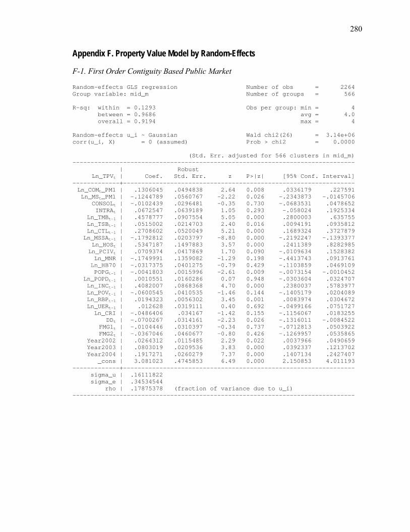
280
Appendix F. Property Value Model by Random-Effects
F-1. First Order Contiguity Based Public Market
Random-effects GLS regression Number of obs = 2264 Group variable: mid_m Number of groups = 566 R-sq: within = 0.1293 Obs per group: min = 4 between = 0.9686 avg = 4.0 overall = 0.9194 max = 4 Random-effects u_i ~ Gaussian Wald chi2(26) = 3.14e+06 corr(u_i, X) = 0 (assumed) Prob > chi2 = 0.0000 (Std. Err. adjusted for 566 clusters in mid_m) ------------------------------------------------------------------------------ | Robust Ln_TPVt | Coef. Std. Err. z P>|z| [95% Conf. Interval] -------------+---------------------------------------------------------------- Ln_COMt_PM1 | .1306045 .0494838 2.64 0.008 .0336179 .227591 Ln_MSt_PM1 | -.1244789 .0560767 -2.22 0.026 -.2343873 -.0145706 CONSOLt | -.0102439 .0296481 -0.35 0.730 -.0683531 .0478652 INTRAt | .0672547 .0639189 1.05 0.293 -.058024 .1925334 Ln_TMBt-1 | .4578777 .0907554 5.05 0.000 .2800003 .635755 Ln_TSBt-1 | .0515002 .0214703 2.40 0.016 .0094191 .0935812 Ln_CTLt-1 | .2708602 .0520049 5.21 0.000 .1689324 .3727879 Ln_MSSAt-1 | -.1792812 .0203797 -8.80 0.000 -.2192247 -.1393377 Ln_HOSt | .5347187 .1497883 3.57 0.000 .2411389 .8282985 Ln_PCIVt | .0709374 .0417869 1.70 0.090 -.0109634 .1528382 Ln_MNR | -.1749991 .1359082 -1.29 0.198 -.4413743 .0913761 Ln_HB70 | -.0317375 .0401275 -0.79 0.429 -.1103859 .0469109 POPGt-1 | -.0041803 .0015996 -2.61 0.009 -.0073154 -.0010452 Ln_POPDt-1 | .0010551 .0160286 0.07 0.948 -.0303604 .0324707 Ln_INCt-1 | .4082007 .0868368 4.70 0.000 .2380037 .5783977 Ln_POVt-1 | -.0600545 .0410535 -1.46 0.144 -.1405179 .0204089 Ln_RBPt-1 | .0194323 .0056302 3.45 0.001 .0083974 .0304672 Ln_UERt-1 | .012628 .0319111 0.40 0.692 -.0499166 .0751727 Ln_CRI | -.0486406 .034167 -1.42 0.155 -.1156067 .0183255 DDt | -.0700267 .0314161 -2.23 0.026 -.1316011 -.0084522 FMG1t | -.0104446 .0310397 -0.34 0.737 -.0712813 .0503922 FMG2t | -.0367046 .0460677 -0.80 0.426 -.1269957 .0535865 Year2002 | .0264312 .0115485 2.29 0.022 .0037966 .0490659 Year2003 | .0803019 .0209536 3.83 0.000 .0392337 .1213702 Year2004 | .1917271 .0260279 7.37 0.000 .1407134 .2427407 _cons | 3.081023 .4745853 6.49 0.000 2.150853 4.011193 -------------+---------------------------------------------------------------- sigma_u | .16111822 sigma_e | .34534544 rho | .17875378 (fraction of variance due to u_i) ------------------------------------------------------------------------------

281
F-2. Second Order Contiguity Based Public Market
Random-effects GLS regression Number of obs = 2264 Group variable: mid_m Number of groups = 566 R-sq: within = 0.1291 Obs per group: min = 4 between = 0.9681 avg = 4.0 overall = 0.9190 max = 4 Random-effects u_i ~ Gaussian Wald chi2(26) = 3.05e+06 corr(u_i, X) = 0 (assumed) Prob > chi2 = 0.0000 (Std. Err. adjusted for 566 clusters in mid_m) ------------------------------------------------------------------------------ | Robust Ln_TPVt | Coef. Std. Err. z P>|z| [95% Conf. Interval] -------------+---------------------------------------------------------------- Ln_COMt_PM2 | .1069473 .0554844 1.93 0.054 -.0018001 .2156948 Ln_MSt_PM2 | -.0913245 .0546485 -1.67 0.095 -.1984336 .0157846 CONSOLt | -.0184088 .0301851 -0.61 0.542 -.0775705 .0407528 INTRAt | .0896003 .0651557 1.38 0.169 -.0381025 .2173031 Ln_TMBt-1 | .4621248 .0914785 5.05 0.000 .2828302 .6414194 Ln_TSBt-1 | .0464902 .0198189 2.35 0.019 .0076459 .0853346 Ln_CTLt-1 | .2794302 .0514509 5.43 0.000 .1785883 .3802721 Ln_MSSAt-1 | -.1878056 .0203411 -9.23 0.000 -.2276734 -.1479377 Ln_HOSt | .5184801 .1526993 3.40 0.001 .2191949 .8177652 Ln_PCIVt | .0684352 .04199 1.63 0.103 -.0138636 .150734 Ln_MNR | -.1748452 .1403692 -1.25 0.213 -.4499638 .1002733 Ln_HB70 | -.0146161 .0436905 -0.33 0.738 -.1002479 .0710157 POPGt-1 | -.0041498 .0015952 -2.60 0.009 -.0072763 -.0010233 Ln_POPDt-1 | -.0072857 .0149977 -0.49 0.627 -.0366807 .0221092 Ln_INCt-1 | .4105715 .087462 4.69 0.000 .2391492 .5819938 Ln_POVt-1 | -.0596334 .0418665 -1.42 0.154 -.1416903 .0224234 Ln_RBPt-1 | .0197828 .0055369 3.57 0.000 .0089307 .0306349 Ln_UERt-1 | .0108319 .0324416 0.33 0.738 -.0527524 .0744162 Ln_CRI | -.0479006 .0353007 -1.36 0.175 -.1170887 .0212874 DDt | -.0686994 .0312212 -2.20 0.028 -.1298918 -.007507 FMG1t | -.0159594 .0324349 -0.49 0.623 -.0795308 .0476119 FMG2t | -.0287357 .0460943 -0.62 0.533 -.1190789 .0616075 Year2002 | .0268142 .0115757 2.32 0.021 .0041262 .0495022 Year2003 | .0808034 .0211561 3.82 0.000 .0393382 .1222686 Year2004 | .1930721 .0244277 7.90 0.000 .1451947 .2409495 _cons | 3.064937 .5662962 5.41 0.000 1.955017 4.174857 -------------+---------------------------------------------------------------- sigma_u | .16362718 sigma_e | .34534419 rho | .18333677 (fraction of variance due to u_i) ------------------------------------------------------------------------------

282
F-3. Distance Based Public Market
Random-effects GLS regression Number of obs = 2264 Group variable: mid_m Number of groups = 566 R-sq: within = 0.1301 Obs per group: min = 4 between = 0.9687 avg = 4.0 overall = 0.9196 max = 4 Random-effects u_i ~ Gaussian Wald chi2(26) = 3.20e+06 corr(u_i, X) = 0 (assumed) Prob > chi2 = 0.0000 (Std. Err. adjusted for 566 clusters in mid_m) ------------------------------------------------------------------------------ | Robust Ln_TPVt | Coef. Std. Err. z P>|z| [95% Conf. Interval] -------------+---------------------------------------------------------------- Ln_COMt_PM3 | .1006165 .0400463 2.51 0.012 .0221272 .1791057 Ln_MSt_PM3 | -.0946486 .0393383 -2.41 0.016 -.1717502 -.017547 CONSOLt | .0071596 .0313745 0.23 0.819 -.0543332 .0686524 INTRAt | .0573687 .0667832 0.86 0.390 -.0735239 .1882614 Ln_TMBt-1 | .4451647 .0902343 4.93 0.000 .2683088 .6220207 Ln_TSBt-1 | .0505844 .0203824 2.48 0.013 .0106356 .0905331 Ln_CTLt-1 | .2728488 .0510939 5.34 0.000 .1727067 .372991 Ln_MSSAt-1 | -.1776936 .0190211 -9.34 0.000 -.2149743 -.1404128 Ln_HOSt | .5446584 .1498667 3.63 0.000 .250925 .8383917 Ln_PCIVt | .0601853 .0383367 1.57 0.116 -.0149534 .1353239 Ln_MNR | -.2217654 .1505936 -1.47 0.141 -.5169234 .0733925 Ln_HB70 | -.045954 .037944 -1.21 0.226 -.1203229 .0284149 POPGt-1 | -.0045649 .001632 -2.80 0.005 -.0077636 -.0013661 Ln_POPDt-1 | -.0486057 .0237682 -2.04 0.041 -.0951906 -.0020209 Ln_INCt-1 | .4054447 .0853562 4.75 0.000 .2381497 .5727398 Ln_POVt-1 | -.0592787 .0416014 -1.42 0.154 -.1408158 .0222585 Ln_RBPt-1 | .0202211 .0055202 3.66 0.000 .0094016 .0310406 Ln_UERt-1 | .0172133 .0326099 0.53 0.598 -.046701 .0811276 Ln_CRI | -.0375233 .0301849 -1.24 0.214 -.0966845 .021638 DDt | -.0641226 .0310497 -2.07 0.039 -.1249788 -.0032663 FMG1t | -.0075282 .0312736 -0.24 0.810 -.0688233 .0537669 FMG2t | -.0280821 .0451281 -0.62 0.534 -.1165316 .0603674 Year2002 | .0265303 .0116642 2.27 0.023 .0036689 .0493918 Year2003 | .0795807 .0214572 3.71 0.000 .0375253 .1216361 Year2004 | .1918297 .0248685 7.71 0.000 .1430884 .240571 _cons | 3.160947 .4518661 7.00 0.000 2.275306 4.046588 -------------+---------------------------------------------------------------- sigma_u | .16044478 sigma_e | .34533919 rho | .17753261 (fraction of variance due to u_i) ------------------------------------------------------------------------------

283
F-4. County Based Public Market
Random-effects GLS regression Number of obs = 2264 Group variable: mid_m Number of groups = 566 R-sq: within = 0.1325 Obs per group: min = 4 between = 0.9725 avg = 4.0 overall = 0.9234 max = 4 Random-effects u_i ~ Gaussian Wald chi2(26) = 3.90e+06 corr(u_i, X) = 0 (assumed) Prob > chi2 = 0.0000 (Std. Err. adjusted for 566 clusters in mid_m) ------------------------------------------------------------------------------ | Robust Ln_TPVt | Coef. Std. Err. z P>|z| [95% Conf. Interval] -------------+---------------------------------------------------------------- Ln_COMt_PM4 | .2138732 .0333084 6.42 0.000 .1485899 .2791565 Ln_MSt_PM4 | -.2167547 .0371445 -5.84 0.000 -.2895565 -.1439529 CONSOLt | .0008167 .0270468 0.03 0.976 -.052194 .0538274 INTRAt | .0006895 .0644809 0.01 0.991 -.1256907 .1270697 Ln_TMBt-1 | .3994896 .087601 4.56 0.000 .2277948 .5711845 Ln_TSBt-1 | .0571463 .0204134 2.80 0.005 .0171367 .0971559 Ln_CTLt-1 | .4006167 .0512972 7.81 0.000 .3000761 .5011573 Ln_MSSAt-1 | -.1151046 .0174804 -6.58 0.000 -.1493657 -.0808436 Ln_HOSt | .5329107 .1358387 3.92 0.000 .2666718 .7991496 Ln_PCIVt | .0698287 .0387465 1.80 0.072 -.0061131 .1457705 Ln_MNR | -.3272805 .1322563 -2.47 0.013 -.586498 -.068063 Ln_HB70 | .0148624 .04122 0.36 0.718 -.0659273 .0956521 POPGt-1 | -.0020638 .0017177 -1.20 0.230 -.0054303 .0013028 Ln_POPDt-1 | -.0262567 .0161605 -1.62 0.104 -.0579307 .0054174 Ln_INCt-1 | .3868774 .0762276 5.08 0.000 .2374741 .5362807 Ln_POVt-1 | -.0732056 .0379344 -1.93 0.054 -.1475558 .0011445 Ln_RBPt-1 | .0181644 .0056556 3.21 0.001 .0070797 .0292492 Ln_UERt-1 | .0236343 .0299983 0.79 0.431 -.0351613 .0824299 Ln_CRI | -.0472273 .0273782 -1.72 0.085 -.1008876 .006433 DDt | -.0581052 .0286032 -2.03 0.042 -.1141664 -.0020439 FMG1t | -.0004449 .0268688 -0.02 0.987 -.0531069 .052217 FMG2t | -.0115541 .0375281 -0.31 0.758 -.0851078 .0619996 Year2002 | .0155105 .0107364 1.44 0.149 -.0055325 .0365536 Year2003 | .0601941 .0225755 2.67 0.008 .0159469 .1044413 Year2004 | .1667353 .0228753 7.29 0.000 .1219006 .21157 _cons | 1.862778 .5401367 3.45 0.001 .80413 2.921427 -------------+---------------------------------------------------------------- sigma_u | .13872006 sigma_e | .3453101 rho | .13895821 (fraction of variance due to u_i) ------------------------------------------------------------------------------

284
Bibliography
Advisory Commission on Intergovernmental Relations (ACIR). 1991. Interjurisdictional Tax and Policy Competition: Good or Bad for the Federal System? Washington, D.C.: ACIR.
Allers, Maarten A. and J. Paul Elhorst. 2005. Tax Mimicking and Yardstick Competition among Local Governments in the Netherlands. International Tax and Public Finance 12(4): 493-513.
Anselin, Luc. 1988. Spatial Econometrics: Methods and Models. Dordrecht: Kluwer.
. 2005. Exploring Spatial Data with GeoDaTM: A Workbook. http://www.csiss.org/clearinghouse/GeoDa/geodaworkbook.pdf. Retrieved Jun 12, 2008.
Anselin, Luc, Anil K. Bera, Raymond Florax, and Mann J. Yoon. 1996. Simple Diagnostic Tests for Spatial Dependence. Regional Science and Urban Economics 26(1): 77-104.
Aronsson, Thomas, Johan Lundberg, and Magnus Wikström. 2000. The Impact of Regional Public Expenditures on the Local Decision to Spend. Regional Science and Urban Economics 30(2): 185-202.
Baiman, S., Demski, J., 1980. Economically Optimal Performance Evaluation and Control Systems. Journal of Accounting Research 18(Supplement): 184-234.
Baird, Robert N. and John H. Landon. 1972. Political Fragmentation, Income Distribution, and the Demand for Government Services. Nebraska Journal of Economics and Business 11(Autumn): 171-184.
Banker, R. D., A. Charnes, and W. W. Cooper. 1984. Some Models for Estimating Technical and Scale Inefficiencies in Data Envelopment Analysis. Management Science 30(9): 1078-1092.
Barro, Robert J. 1973. The Control of Politicians: An Economic Model. Public Choice 14(1): 19-42.
Bates, Laurie J. and Rexford E. Santerre. 2006. Leviathan in the Crosshairs. Public Choice 127(1): 133-145.
Baum, C. F., M. E. Schaffer, and S. Stillman. 2007. ivreg2: Stata Module for Extended Instrumental Variables/2SLS, GMM and AC/HAC, LIML, and k-class regression. Boston College Department of Economics, Statistical Software Components S425401. http://ideas.repec.org/c/boc/bocode/s425401.html. Retrieved Jun 12, 2008.
Beck, John H. 1993. Tax Abatement and Tax Rates in a System of Overlapping Revenue-Maximizing Governments. Regional Science & Urban Economics 23(5): 645-665.
Beck, N., and J. N. Katz. 1995. What to Do (and Not to Do) with Time-Series Cross-Section Data. American Political Science Review 89: 634–647.

285
Belleflamme, Paul and Jean Hindriks. 2005. Yardstick Competition and Political Agency Problems. Social Choice & Welfare 24(1): 155-169.
Benecke, Robert. 2004a. Municipal Finance Administration in New Jersey. NJ: Center for Government Services, Rutgers.
. 2004b. The Municipal Budget Process. NJ: Center for Government Services, Rutgers.
Besley, Timothy and Anne Case. 1995. Incumbent Behavior: Vote-seeking, Tax-setting, and Yardstick Competition. American Economic Review 85(1): 25-45.
Besley, Timothy and Harvey S. Rosen. 1998. Vertical Externalities in Tax Setting: Evidence from Gasoline and Cigarettes. Journal of Public Economics 70(3): 383-398.
Besley, Timothy and Michael Smart. 2002. Does Tax Competition Raise Voter Welfare? CEPR Discussion Paper No. 3131.
Bivand, Roger and Stefan Szymanski. 2000. Modelling the Spatial Impact of the Introduction of Compulsive Competitive Tendering. Regional Science and Urban Economics 30(2): 203-219.
Boadway, Robin and Michael Keen. 1996. Efficiency and the Optimal Direction of Federal-State Transfers. International Tax and Public Finance 3(2): 137-155.
Boots, Barry and Michael Tiefelsdorf. 2000. Global and Local Spatial Autocorrelation in Bounded Regular Tessellations. Journal of Geographical Systems 2(4): 319-348.
Bordignon, Massimo, Floriana Cerniglia, and Federico Revelli. 2003. In Search of Yardstick Competition: A Spatial Analysis of Italian Municipality Property Tax Setting. Journal of Urban Economics 54(2): 199-217.
Bosch, Núria and Albert Solé-Ollé. 2007. Yardstick Competition and the Political Costs of Raising Taxes: An Empirical Analysis of Spanish Municipalities. International Tax and Public Finance 14(1): 71-92.
Boyne, George A. 1992. Local Government Structure and Performance: Lessons from America? Public Administration 70(3): 333-357.
Braun, Peter J. 2002. The Role of the Governing Body in Municipal Finance. In Cupano, Kathleen McKenzie and Mellany Alio Eds. Powers and Duties of the Municipal Governing Body. NJ: Center for Government Services, Rutgers.
Brennan, Geoffrey and James Buchanan. 1980. The Power to Tax: Analytical Foundations of a Fiscal Constitution. NY: Cambridge University Press.
Brett, Craig and Joris Pinkse. 2000. The Determinants of Municipal Tax Rates in British Columbia. Canadian Journal of Economics 33(3): 695-714.
Brueckner, Jan K. 1979. Property Values, Local Public Expenditure, and Economic Efficiency. Journal of Public Economics 11(2): 223-245.
. 1982. A Test of Allocative Efficiency in the Local Public Sector. Journal of Public Economics 19(3): 311-331.

286
. 1998. Testing for Strategic Interaction among Local Governments: The Case of Growth Controls. Journal of Urban Economics 44(3): 438-467.
. 2000. A Tiebout/Tax-Competition Model. Journal of Public Economics 77(2): 285-306.
. 2003. Strategic Interaction among Governments: An Overview of Empirical Studies. International Regional Science Review 26(2): 175-188.
. 2004. Fiscal Decentralization with Distortionary Taxation: Tiebout vs. Tax Competition. International Tax and Public Finance 11(2): 133-153.
Brueckner, Jan K. and Luz A. Saavedra. 2001. Do Local Governments Engage in Strategic Property-Tax Competition? National Tax Journal 54(2): 203-229.
Brueckner, Jan K. and Thomas L. Wingler. 1984. Public Intermediate Inputs, Property Values, and Allocative Efficiency. Economic Letters 14(2-3): 245-250.
Brülhart, Marius and Mario Jametti. 2006. Vertical versus Horizontal Tax Externalities: An Empirical Test. Journal of Public Economics 90(10-11): 2027-2062.
Bucovetsky, Sam. 1991. Asymmetric Tax Competition. Journal of Urban Economics 30(2): 167-181.
Bucovetsky, Sam and John Douglas Wilson, 1991. Tax Competition with Two Instruments. Regional Science and Urban Economics 21(3): 333-350.
Buettner, Thiess. 2003. Tax Base Effects and Fiscal Externalities of Local Capital Taxation: Evidence from a Panel of German Jurisdictions. Journal of Urban Economics 54(1): 110-128.
Campbell, Rebecca J. 2004. Leviathan and Fiscal Illusion in Local Government Overlapping Jurisdictions. Public Choice 120(3-4): 301-329.
Case, Anne. 1993. Interstate Tax Competition after TRA86. Journal of Policy Analysis & Management 12(1): 136-148.
Center for Government Services. 2001-2006. New Jersey Legislative District Data Book. NJ: Center for Local Government Services, Rutgers.
Charnes, A, W.W. Cooper, and E. Rhodes. 1978. Measuring the Efficiency of Decision Making Units. European Journal of Operational Research 2(6): 429-444.
Charnes, Chris, William W. Cooper, Arie Y. Lewin, and Lawrence M. Seiford. Eds. 1995. Data Envelopment Analysis: Theory, Methodology, and Applications. NJ: Springer.
Chicoine, David L. and Norman Walzer. 1985. Governmental Structure and Local Public Finance. MA: Oelgeschlager, Gunn, and Hain Publishers.
Cope, Stephen. 2000. Assessing Rational-Choice Models of Budgeting-From Budget-Maximizing to Bureau-Shaping: A Case Study of British Local Government. Journal of Public Budgeting, Accounting & Financial Management 12(4): 598-624.
287
Crone, Theodore M. 1998/1999. Using State Indexes to Define Economic Regions in the U.S. Journal of Economic and Social Measurement 25(3-4): 259-275.
Dahlby, Bev. 1996. Fiscal Externalities and the Design of Intergovernmental Grants. International Tax and Public Finance 3(3): 397-412.
Dahlby, Bev and Leonard S. Wilson. 2003. Vertical Fiscal Externalities in a Federation. Journal of Public Economics 87(5-6): 917-930.
De Boger, Bruno and Kristiaan Kerstens. 1996a. Cost Efficiency of Belgian Local Governments: A Comparative Analysis of FDH, DEA, and Econometric Approaches. Regional Science and Urban Economics 26(2): 145-170.
. 1996b. Radial and Nonradial Measures of Technical Efficiency: An Empirical Illustration for Belgian Local Governments Using an FDH Reference Technology. The Journal of Productivity Analysis 7(1): 41-62.
. 2000. What Is Known about Municipal Efficiency? The Belgian Case and Beyond. In J. Blank Ed. Public Provision and Performance: Contributions from Efficiency and Productivity Measurement. Amsterdam: Elsevier. pp. 299-330.
De Borger et al. 1994. Explaining Differences in Productive Efficiency: An Application to Belgian Municipalities. Public Choice 80(3-4): 339-358.
Deller, Steven C. 1990. An Application of a Test for Allocative Efficiency in the Local Public Sector. Regional Science and Urban Economics 20(3): 395-406.
Deller, Steven C. and David L. Chicoine. 1993. Representative versus Direct democracy: A Test of Allocative Efficiency in Local Government Expenditures. Public Finance Quarterly 21(1): 100-114.
Devereux, M. P., B. Lockwood, and M. Redoano. 2007. Horizontal and Vertical Indirect Tax Competition: Theory and Some Evidence from the USA. Journal of Public Economics 91(3-4): 451-479.
Dollery, Brian E., Joe L. Wallis, and Andrew Worthington. 2001. The Empirical Measure of Local Government Efficiency. In Dollery, Brian E. and Joe L. Wallis Eds. The Political Economy of Local Government. MA: Edward Elgar. pp. 71-113.
Dowding, Keith, Peter John, and Stephen Biggs. 1994. Tiebout: A Survey of the Empirical Literature. Urban Studies 31(4-5): 767-797.
Downs, Anthony. 1957. An Economic Theory of Democracy. NY: Harper and Row.
Dye, Thomas R. 1990. American Federalism: Competition among Governments. MA: Lexington Books.
Eberts, Randall W. and Timothy J. Gronberg. 1988. Can Competition Among Local Governments Constrain Government Spending? Economic Review - Federal Reserve Bank of Cleveland. 24(1): 2-9.
. 1990. Structure, conduct, and Performance in the Local Public Sector. National Tax Journal 43(2): 165-173.
Edwards, Jeremy and Michael Keen. 1996. Tax competition and Leviathan. European Economic Review 40(1): 113-134.

288
Egger, Peter, Michael Pfaffermayr, and Hannes Winner. 2005. An Unbalanced Spatial Panel Data Approach to US State Tax Competition. Economics Letters 88(3): 329-335.
Epple, Dennis and Allan Zelenitz. 1981. The Implications of Competition among Jurisdictions: Does Tiebout Need Politics? Journal of Political Economy 89(6): 1197-1217.
Esteller-Moré, Álex and Albert Solé-Ollé. 2001. Vertical Income Tax Externalities and Fiscal Interdependence: Evidence from the US. Regional Science and Urban Economics 31(2-3): 247-272.
Farrell, M. J. 1957. The Measurement of Productive Efficiency. Journal of the Royal Statistical Society 120(3): 253-289.
Feld, Lars P. and Gebhard Kirchgässner. 2001. The Political Economy of Direct Legislation: Direct Democracy and Local Decision-Making. Economic Policy 16(33): 329-357.
Ferejohn, John. 1986. Incumbent Performance and Electoral Control. Public Choice 50(1): 5-26.
Fiorina, Morris P. 1981. Retrospective Voting in American National Elections. CT: Yale University Press.
Fisher, Ronald C. and Leslie E. Papke. 2000. Local Government Responses to Education Grants. National Tax Journal 53(1): 153-168.
Flochel, Laurent and Thierry Madies. 2002. Interjurisdictional Tax Competition in a Federal System of Overlapping Revenue Maximizing Governments. International Tax and Public Finance 9(2): 121-141.
Flowers, Marilyn R. 1988. Shared Tax Sources in a Leviathan Model of Federalism. Public Finance Quarterly 16(1): 67-77.
Forbes, Kevin F. and Ernest M. Zampelli. 1989. Is Leviathan a Mythical Beast? American Economic Review 79(3): 568-577.
Fredriksson, Per G. and Daniel L. Millimet. 2002. Strategic Interaction and the Determination of Environmental Policy across U.S. States. Journal of Urban Economics 51(1): 101-122.
Freitag, Markus and Adrian Vatter. 2006. Initiatives, Referendums, and the Tax State. Journal of European Public Policy 13(1): 89-112.
Gramlich, E. M. 1977. Intergovernmental Grants: A Review of the Empirical Literature. In Wallas E. Oates ED. The Political Economy of Fiscal Federalism. MA: Lexington Books. pp. 219-239.
Goodspeed, Timothy J. 2000. Tax Structure in a Federation. Journal of Public Economics 75(3): 493-506.
Grossman, Philip J., Panayiotis Mavros, and Robert W. Wassmer. 1999. Public Sector Technical Inefficiency in Large U.S. Cities. Journal of Urban Economics 46 (2): 278-299.
289
Hayashi, Masayoshi and Robin Boadway. 2001. An Empirical Analysis of Intergovernmental Tax Interaction: The Case of Business Income Taxes in Canada. Canadian Journal of Economics 34(2): 481-503.
Hayes, Kathy J., Laura Razzolini, and Leola B. Ross. 1998. Bureaucratic Choice and Nonoptimal Provision of Public Goods: Theory and Evidence. Public Choice 94(1-2): 1-20.
Hendrick, Rebecca, Yonghong Wu, and Benoy Jacob. 2007. Tax Competition among Municipal Governments: Exit vs. Voice. Urban Affairs Review 43(2): 221-255).
Hernández-Murillo, Rubén. 2003. Strategic Interaction in Tax Policies among States. Review-Federal Reserve Bank of St. Louis 85(3): 47-56.
Heyndels, Bruno and Jef Vuchelen. 1998. Tax Mimicking among Belgian Municipalities. National Tax Journal 51(1): 89-101.
Hirschman, Albert O. 1970. Exit, Voice, and Loyalty: Responses to Decline in Firms, Organizations, and States. Cambridge, Massachusetts: Harvard University Press.
Holmström, Bengt. 1982. Moral Hazard in Teams. The Bell Journal of Economics 13(2): 324-340.
Hoyt, William H. 1991. Property Taxation, Nash Equilibrium, and Market Power. Journal of Urban Economics 30(1): 123-131.
Hughes, P. A. Nold and Mary E. Edwards. 2000. Leviathan vs. Lilliputian: A Data Envelopment Analysis of Government Efficiency. Journal of Regional Science 40(4): 649-669.
Kanbur, R. and M. Keen. 1993. Jeux Sans Fontières: Tax Competition and Tax Coordination When Countries Differ in Size. The American Economic Review 83(4): 877-892.
Karcher, Alan J. 1998. New Jersey’s Multiple Municipal Madness. NJ: Rutgers University Press.
Keen, Michael J. 1998. Vertical Tax Externalities in the Theory of Fiscal Federalism. International Monetary Fund Staff Papers 45(3): 454-484.
Keen, Michael J. and Christos Kotsogiannis. 2002. Does Federalism Lead to Excessively High Taxes? American Economic Review 92(1): 363-370.
. 2003. Leviathan and Capital Tax Competition in Federations. Journal of Public Economic Theory 5(2): 177-199.
Kelejian, Harry H and Ingmar R. Prucha. 1997. Estimation of Spatial Regression Models with Autoregressive Error by Two Stage Least Squares: A Serious Problem. International Regional Science Review 20(): 103–111.
. 1999. A Generalized Moments Estimator for the Autoregressive Parameter in a Spatial Model. International Economic Review 40(2): 509-533.
Key, V.O., Jr. 1966. The Responsible Electorate. MA: Harvard University Press.

290
Kincaid, John. 1991. The Competitive Chalange to Cooperative Federalism: A Theory of Federal Democracy. In Kenyon, Daphne A. and John Kincaid Eds. Competition among States and Local Governments: Efficiency and Equity in American Federalism. Washington, D.C.: The Urban Institute Press. pp. 87-114.
Klick, Jonathan and Francesco Parisi. 2005. Intra-Jurisdictional Tax Competition. Constitutional Political Economy 16(4): 387-395.
Inman, Robert P. 1979. The Fiscal Performance of Local Governments: An Interpretative Review. In Mieszkowski, Peter and Mahlon Straszheim Eds. Current Issues in Urban Economics. Maryland: The Johns Hopkins University Press. pp.270-321.
Ladd, Helen F. 1992. Mimicking of Local Tax Burdens among Neighboring Counties. Public Finance Quarterly 20(4): 450-467.
Lazear, Edward P. and Sherwin Rosen. 1981. Rank-order Tournaments as Optimum Labor Contracts. Journal of Political Economy 89(5): 841-864.
Luna, Learnt. 2004. Local Sales Tax Competition and the Effect on County Governments’ Tax Rates and Tax Bases. Journal of the American Taxation Association 26(1): 43-61.
Mahalanobis, P.C. 1930. On Tests and Measures of Group Divergence. Journal of the Asiatic Society of Bengal 26: 541-588.
Matsusaka, John G. 1995. Fiscal Effects of the Voter Initiative: Evidence from the Last 30 Years. The Journal of Political Economy 103(3): 587-623.
Mieszkowski, Peter and George R. Zodrow. 1989. Taxation and the Tiebout Model: The Differential Effects of Head Taxes, Taxes on Land Rents, and Property Taxes. Journal of Economic Literature 27(3): 1098-1146.
Migué, Jean-Luc and Gérard Bélanger. 1974. Toward a General Theory of Managerial Discretion. Public Choice 17(1): 27-43.
Mintz, Jack and Henry Tulkens. 1986. Commodity Tax Competition between Member States of a Federation: Equilibrium and Efficiency. Journal of Public Economics 29(2): 133-172.
Moran, P.A.P. 1950. Notes on Continuous Stochastic Phenomena. Biometrika 37: 17-33.
Mueller, Dennis C. 2003. Public Choice III. Cambridge: Cambridge University Press
Musgrave, Richard. 1959. The Theory of Public Finance: A Study in Public Economy. NY: McGraw-Hill.
Nelson, Michael A. 1987. Searching for Leviathan: Comment and Extension. American Economic Review 77(1): 198-204.
New Jersey Department of Education (NJ DOE). 2000-01 ~ 2007-08. State Aid Summaries. http://www.nj.gov/education/stateaid/. Retrieved December 16, 2008.
. 2007. New Jersey Vital Education Statistics 2005-06. http://www.nj.gov/education/data/vitaledtoc.htm. Retrieved December 16, 2008.

291
New Jersey Department of Labor and Workforce Development. 2000-2007. Population and Household Estimates. http://lwd.dol.state.nj.us/labor/lpa/dmograph/est/est_index.html. Retrieved December 16, 2008.
New Jersey Division of Finance, Department of Education. 2008. Budget Guidelines: Fiscal Year 2008-09. http://www.nj.gov/education/finance/fp/audit/0708/guide/guidelines.pdf. Retrieved December 16, 2008.
New Jersey Division of Local Government Services, Department of Community Affairs (NJ DLGS). 1994. Annual Report of the Division of Local Government Services. NJ: NJ DLGS.
. 2004-05. Municipal Government Financial Information Summaries. http://www.state.nj.us/dca/lgs/annualrpt/armenu.shtml. Retrieved December 16, 2008.
. 2000-2007a. Property Tax Information. http://www.state.nj.us/dca/lgs/taxes/taxmenu.shtml. Retrieved December 16, 2008
. 2000-2007b. State Aid to Municipalities. http://www.state.nj.us/dca/lgs/muniaid/aidmenu.shtml. Retrieved December 16, 2008
New Jersey Division of Taxation, Department of Treasury. 2001. Handbook for New Jersey Assessors. NJ: New Jersey Division of Taxation.
New Jersey Office of Legislative Services, State Legislature (NJ OLS). 2005. The Assessment of Real Property: Answers to Frequently Asked Questions. OLS Background Report No. 119. http://www.njleg.state.nj.us/PropertyTaxSession/OPI/bg119.pdf. Retrieved December 16, 2008.
New Jersey Statutes Annotated (N.J.S.A.) 18A:7F-38 to 41.
N.J.S.A. 18A:17-14.1.
N.J.S.A. 18A:17-15.
N.J.S.A. 18A:17-31 to 36.
N.J.S.A. 18A:9-2 to 3.
N.J.S.A. 18A:9-4 to 6.
N.J.S.A. 40:103-5(71).
N.J.S.A. 40:41A-2 et seq.
N.J.S.A. 40:69A-1 et seq.
N.J.S.A. 40:70-1 et seq.
N.J.S.A. 40:79-1 et seq.
N.J.S.A. 40:103-5(71).

292
N.J.S.A. 40A:4-1 et seq.
N.J.S.A. 40A:4-45.1 et seq.
N.J.S.A. 40A:60-1 et seq.
N.J.S.A. 40A:6-1.
N.J.S.A. 40A:61-1 et seq.
N.J.S.A. 40A:62-1 et seq.
N.J.S.A. 40A:63-1 et seq.
N.J.S.A. 40A:63-8 et seq.
N.J.S.A. 54:1.35.3.
N.J.S.A. 54:3-17 et seq.
N.J.S.A. 54:4-2.25.
N.J.S.A. 54:4-23.
Niskanen, William A. 1971. Bureaucracy and Representative Government. Chicago: Aldine.
. 1975. Bureaucrats and Politicians. Journal of Law and Economics 18(3): 617-644.
. 1978. Competition among Government Bureaus. In Buchanan et al. Eds. The Economics of Politics. London: Institute of Economic Affairs.
. 1991. A Reflection on Bureaucracy and Representative Government. In Blais, Andre and Stephane Dion. Eds. The Budget-Maximizing Bureaucrat: Appraisals and Evidence. PA: University of Pittsburgh Press. pp. 13-31.
Oates, Wallace E. 1969. The Effects of Property Taxes and Local Public Spending on Property Values: An Empirical Study of Tax Capitalization and the Tiebout Hypothesis. Journal of Political Economy 77(6): 957-971.
. 1972. Fiscal Federalism. New York: Harcourt Brace Jovanovich.
. 1985. Searching for Leviathan: An Empirical Study. American Economic Review 75(4): 748-757.
Olson, Mancur. 1969. The Principle of Fiscal Equivalence: The Division of Responsibilities among Different Levels of Government. American Economic Review 59(2): 479-487.
Pareti, Alice Anne. 2001. Principles of Municipal Tax Collection I. NJ: Center for Government Services, Rutgers.
Raimondo, Henry J. 1992. Economics of State and Local Government. NY: Praeger.
Rauscher, Michael. 1998. Leviathan and Competition among Jurisdictions: The Case of Benefit Taxation. Journal of Urban Economics 44(1): 59-67.
293
Regional Plan Association. 2005. Fundamental Property Tax Reform: Land Use Implications of New Jersey’s Tax Debate. http://www.rpa.org/pdf/propertytax101705.pdf. Retrieved December 16, 2008.
Reock, Ernest C. 1994. Long Range Property Tax Rate Trends in New Jersey: 1954-1993. NJ: Center for Government Services, Rutgers.
. 2002. Forms of Municipal Governments in New Jersey. In Cupano, Kathleen McKenzie and Mellany Alio Eds.Powers and Duties of the Municipal Governing Body. NJ: Center for Government Services, Rutgers.
Revelli, Federico. 2001. Spatial Patterns in Local Taxation: Tax Mimicking or Error Mimicking? Applied Economics 33(9): 1101-1107.
. 2002a. Local Taxes, National Politics and Spatial Interactions in English District Election Results. European Journal of Political Economy 18(2): 281-299.
. 2002b. Testing the Tax Mimicking versus Expenditure Spill-over Hypotheses Using English Data. Applied Economics 34(14): 1723-1731.
. 2003. Reaction or Interaction? Spatial Process Identification in Multi-tiered Government Structures. Journal of Urban Economics 53(1): 29-53.
. 2006. Performance Rating and Yardstick Competition in Social Service Provision. Journal of Public Economics 90(3): 459-475.
Saavedra, Luz Amparo. 2000. A Model of Welfare Competition with Evidence from AFDC. Journal of Urban Economics 47(2): 248-279.
Salmon, Pierre. 1987. Decentalisation as an Incentive Scheme. Oxford Review of Economic Policy 3(2): 24-43.
Samuelson, Paul. A. 1954. The Pure Theory of Public Expenditures. Review of Economics and Statistics 36(4): 387-389.
Santerre, Rexford E. 1986. Representative versus Direct Democracy: A Tiebout Test of Relative Performance. Public Choice 48(1): 55-63.
Schaltegger, Christoph A. and Dominique Küttel. 2002. Exit, Voice, and Mimicking Behavior: Evidence from Swiss Cantons. Public Choice 113(1-2): 1-23.
Schneider, Mark. 1989. Intermunicipal Competition, Budget Maximizing Bureaucrats, and the Level of Suburban Competition. American Journal of Political Science 33(3): 612-628.
Shah, Anwar M. 1992. Empirical Tests for Allocative Efficiency in the Local Public Sector. Public Finance Quarterly 20(3): 359-377.
. 1994. The Reform of Intergovernmental Fiscal Relations in Developing and Emerging Market Economies. Washington, D.C.: World Bank.
Shephard, R. W. 1970. Theory of Cost and Production Function. NJ: Princeton University Press.
Shleifer, Andrei. 1985. A Theory of Yardstick Competition. The RAND Journal of Economics 16(3): 319-327.
294
Sigelman, Lee. 1986. The Bureaucrats as Budget Maximizer: An Assumption Examined. Public Budgeting and Finance 6(1): 50-59
Silkman, Richard and Dennis R. Young. 1982. X-Efficiency and State Formula Grants. National Tax Journal 35(3): 383-397.
Solé-Ollé, Albert. 2003. Electoral Accountability and Tax Mimicking the Effects of Electoral Margins, Coalition, Government Ideology. European Journal of Political Economy 19(4): 685-713.
. 2006. Expenditure Spillovers and Fiscal Interactions: Empirical Evidence from Local Governments in Spain. Journal of Urban Economics 59(1): 32-53.
Special Session Joint Legislative Committee on Constitutional Reform and Citizens Property Tax Constitutional Convention (SSJLCCR). 2006. Constitutional Reform and Citizens Property Tax Constitutional Convention Final Report. http://www.njleg.state.nj.us/PropertyTaxSession/OPI/jccr_final_report.pdf. Retrieved December 16, 2008.
Stansel, Dean. 2006. Interjurisdictional Competition and Local Government Spending in U.S. Metropolitan Areas. Public Finance Review 34(2): 173-194.
Stigler, George. 1957. The Tenable Range of Functions of Local Government. In Joint Economic Committee, Subcommittee on Fiscal Policy, U.S. Congress Eds. Federal Expenditure Policy for Economic Growth and Stability. Washington, D.C.: U.S. Government Printing Office. pp. 213-219.
Tax Foundation. 2008. State and Local Property Tax Collections per Capita and per Household, Fiscal Year 2006. http://www.taxfoundation.org/files/state&local_proptaxcoll_pc&ph-20080630.pdf. Retrieved December 16, 2008.
Taylor, Lori L. 1995. Allocative Efficiency and Local Government. Journal of Urban Economics 37(2): 201–211.
Thanassoulis, Emmanuel. 2001. Introduction to the Theory and Application of Data Envelopment Analysis: A Foundation Text with Integrated Software. Norwell, MA: Kluwer Academic Publishers.
Tiebout, Charles. 1956. A Pure Theory of Local Expenditures. Journal of Political Economy 64: 431-455.
Turnbull, Geoffrey K. and Salpie S. Djoundourian. 1993. Overlapping Jurisdictions: Substitutes or Complements? Public Choice 75(3): 231-245.
U.S. Census Bureau, 2001. Annual Geographical Mobility Rates, by Type of Movement: 1947-2000. http://www.census.gov/population/www/socdemo/migrate.html. Retrieved February 15, 2008.
. 2003-04 ~ 2005-06. State and Local Government Finances. http://www.census.gov/govs/www/estimate.html. Retrieved December 16, 2008.

295
. 2007. Population Density for States and Puerto Rico. http://www.census.gov/popest/gallery/maps/popsize-2007.html. Retrieved December 16, 2008.
Vermeir, Jan and Bruno Heyndels. 2006. Tax Policy and Yardstick Voting in Flemish Municipal Elections. Applied Economics 38(19): 2285-2297.
Von Hagen, Jürgen and Ian Harden. 1996. Budget Processes and Commitment to Fiscal Discipline. IMF Working Paper.
Wagoner, Charles B. 1995. Local Fiscal Competition: An Intraregional Perspective. Public Finance Quarterly 23(1): 95-114.
Wetzel, Heike. 2006. Economies of Scope in European Railways: An Efficiency Analysis. Halle Institute for Economic Research. IWH-Discussion Papers No. 5.
Wildasin, David E. 1986. Interstate Tax Competition: A Comment. National Tax Journal 39(3): 353-356.
. 1988. Nash Equilibria in Models of Fiscal Competition. Journal of Public Economics 35(2): 229-240.
. 1989. Interjurisdictional Capital Mobility: Fiscal Externality and a Corrective Subsidy. Journal of Urban Economics 25(2):193-212.
Wilson, John Douglas. 1986. A Theory of Interregional Tax Competition. Journal of Urban Economics 19(3): 296-316.
. 1991. Tax Competition with Interregional Differences in Factor Endowments. Regional Science and Urban Economics 21(3): 423-451.
. 1995. Mobile Labor, Multiple Tax Instruments, and Tax Competition. Journal of Urban Economics 38(3): 333-356.
. 1999. Theories of Tax Competition. National Tax Journal 52(2): 269-304.
. 2005. Welfare-Improving Competition for Mobile Capital. Journal of Urban Economics 57(1): 1-18.
Wilson, John Douglas and R. H. Gordon. 2003. Expenditure Competition. Journal of Public Economic Theory 5(2): 399-417.
Wilson, P. W. 2007. FEAR: A Package for Frontier Efficiency Analysis with R. Socio-Economic Planning Sciences. Forthcoming. http://www.clemson.edu/economics/faculty/wilson/Software/FEAR/FEAR-1.1/fear-1.1_user_guide.pdf. Retrieved October 10, 2008.
Woodbury, Kim and Brian Dollery. 2004. Efficiency Measurement in Australian Local Government: The Case of New South Wales Municipal Water Services. Review of Policy Research 21(5): 615-636.
Worthington, Andrew. 2000. Cost Efficiency in Australian Local Government: A Comparative Analysis of Mathematical Programming and Econometric Approaches. Financial Accountability and Management 16(3): 201-224.

296
Wrede, Matthias. 2000. Shared Tax Sources and Public Expenditures. International Tax and Public Finance 7(2): 163-175.
. 2001. Yardstick Competition to Tame the Leviathan. European Journal of Political Economy 17(4): 705-721.
Zax, Jeffrey S. 1989. Is There a Leviathan in Your Neighborhood? American Economic Review 79(3): 560-567.
Zodrow, George R. and Peter Mieszkowski. 1986. Pigou, Tiebout, Property Taxation, and the Underprovision of Local Public Goods. Journal of Urban Economics 19(3): 356-370.

297
Curriculum Vitae
Name : Lee, Sock Hwan
Date of Birth : January 10, 1970
Place of Birth : Republic of Korea
Education
1989-1996 : Hanyang University, Seoul, Korea. B.A. in Public Administration
1997-1999 : Hanyang University, Seoul, Korea. M.A. in Public Administration
Experience 2001-2004 : Researcher,
Seoul Development Institute, Seoul, Korea
2002-2004 : Researcher and Lecturer, Mirae Knowledge Works, Seoul, Korea
2005-2007 : Teaching Assistant, Department of Public Administration, Rutgers-Newark
Awards
2007-2008 : Graduate Fellowship, Graduate School-Newark, Rutgers
Publications
Tae Ho Eom and Sock Hwan Lee. 2006. Court-Mandated Education Finance Reform on School Districts’ Efficiency: Case of New Jersey. Proceedings of National Tax Association’s 98th Annual Conference on Taxation. pp. 11-18.
Tae Ho Eom, Sock Hwan Lee, and Hau Xu. 2008. Introduction to Panel Data Analysis: Concepts and Practices. In Yang, Kaifeng and Gerald J. Miller. Eds. Handbook of Research Methods in Public Administration. 2nd ed. pp.575-594.
Tae Ho Eom and Sock Hwan Lee. Efficiency Implications of Court-Mandated Education Finance Reform in New Jersey. Policy Studies Journal (in revising).