计算机辅助几何设计 2021秋学期 Bézier Curves

Bézier Curves

陈仁杰

中国科学技术大学

计算机辅助几何设计2021秋学期

Bézier curves

• Bézier curves/splines developed by• Paul de Casteljau at Citroen (1959)

• Pierre Bézier at Renault (1963)

for free-form parts in automotive design

Bézier curves

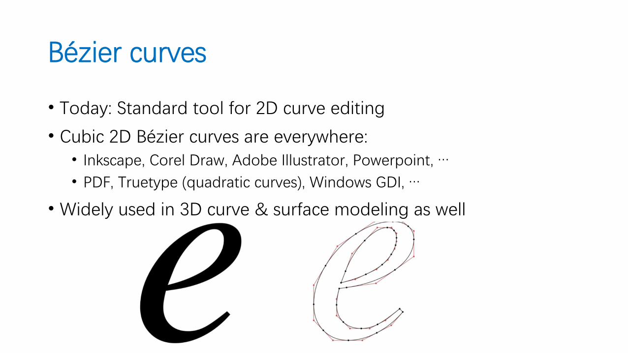
• Today: Standard tool for 2D curve editing

• Cubic 2D Bézier curves are everywhere:• Inkscape, Corel Draw, Adobe Illustrator, Powerpoint, …

• PDF, Truetype (quadratic curves), Windows GDI, …

• Widely used in 3D curve & surface modeling as well

Curve representation

• The implicit curve form 𝑓 𝑥, 𝑦 = 0 suffers from several limitations:

Curve representation

• The implicit curve form 𝑓 𝑥, 𝑦 = 0 suffers from several limitations:

• Multiple values for the same 𝑥-coordinates

• Undefined derivative 𝑑𝑦

𝑑𝑥(see blue cross)

• Not invariant w.r.t axes transformations

Parametric representation

• Remedy: parametric representation 𝑐 𝑡 = 𝑥 𝑡 , 𝑦 𝑡

• Easy evaluations

• The parameter 𝑡 can be interpreted as time

• The curve can be interpreted as the path traced by a moving particle

Modeling with the power basis, …

• Example of a parabola: 𝒇 𝑡 = 𝒂𝑡2 + 𝒃𝑡 + 𝒄

𝒇 𝑡 =11

𝑡2 +−20

𝑡 +10

Modeling with the power basis, …no thanks!• Examples of a parabola: 𝒇 𝑡 = 𝒂𝑡2 + 𝒃𝑡 + 𝒄: the coefficients of

the power basis lack intuitive geometric meaning

Back to the drawing board

• A point on a parametric line

𝒃𝟏

𝒃𝟎

𝒃𝟎𝟏

𝒃𝟎𝟏 = 1 − 𝑡 𝒃𝟎 + 𝑡𝒃𝟏


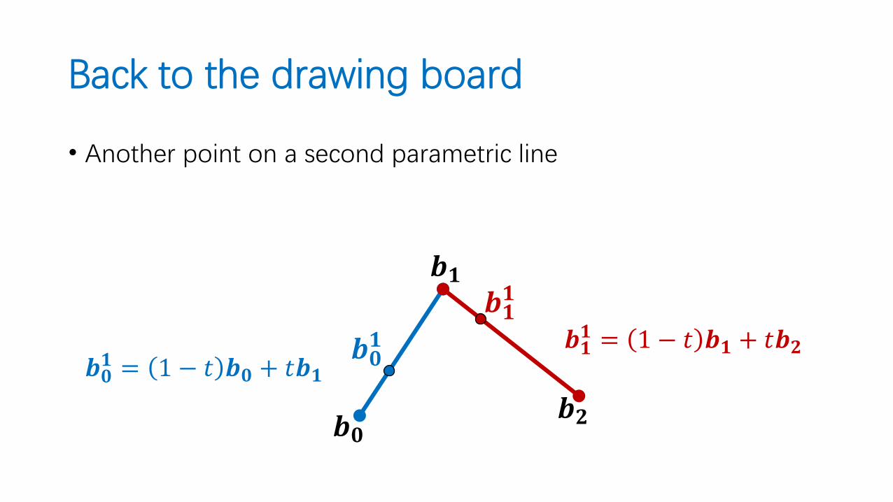
• Another point on a second parametric line

𝒃𝟏𝟏 = 1 − 𝑡 𝒃𝟏 + 𝑡𝒃𝟐

𝒃𝟎𝟏 = 1 − 𝑡 𝒃𝟎 + 𝑡𝒃𝟏

𝒃𝟏

𝒃𝟎𝒃𝟐

𝒃𝟏𝟏

𝒃𝟎𝟏


• A third point on the line defined by the first two points

𝒃𝟏

𝒃𝟎𝒃𝟐

𝒃𝟏𝟏

𝒃𝟎𝟏

𝒃𝟎𝟐

𝒃𝟎𝟐 = 1 − 𝑡 𝒃𝟎

𝟏 + 𝑡𝒃𝟏𝟏

𝒃𝟏𝟏 = 1 − 𝑡 𝒃𝟏 + 𝑡𝒃𝟐

𝒃𝟎𝟏 = 1 − 𝑡 𝒃𝟎 + 𝑡𝒃𝟏


• And then simplify…

𝒃𝟎𝟏 = 1 − 𝑡 𝒃𝟎 + 𝑡𝒃𝟏

𝒃𝟎𝟐 = 1 − 𝑡 𝒃𝟎

𝟏 + 𝑡𝒃𝟏𝟏

𝒃𝟏𝟏 = 1 − 𝑡 𝒃𝟏 + 𝑡𝒃𝟐

𝒃𝟎𝟐 = 1 − 𝑡 1 − 𝑡 𝒃𝟎 + 𝑡𝒃𝟏 + 𝑡 1 − 𝑡 𝒃𝟏 + 𝑡𝒃𝟐

𝒃𝟎𝟐 = 1 − 𝑡 2𝒃𝟎 + 2𝑡 1 − 𝑡 𝒃𝟏 + 𝑡2𝒃𝟐

𝒃𝟏

𝒃𝟎𝒃𝟐

𝒃𝟏𝟏

𝒃𝟎𝟏

𝒃𝟎𝟐


• We obtained another description of parabolic curves

• The coefficients 𝒃𝟎, 𝒃𝟏, 𝒃𝟐 have a geometric meaning

𝒃𝟎𝟐 = 1 − 𝑡 2𝒃𝟎 + 2𝑡 1 − 𝑡 𝒃𝟏 + 𝑡2𝒃𝟐

𝒃𝟏

𝒃𝟎𝒃𝟐

𝒃𝟏𝟏

𝒃𝟎𝟏

𝒃𝟎𝟐

Example re-visited

• Let’s rewrite our initial parabolic curve example in the new basis

𝒇 𝑡 =11

𝑡2 +−20

𝑡 +10

𝒇 𝑡 =10

1 − 𝑡 2 +00

2𝑡 1 − 𝑡 +01

𝑡2

Example re-visited

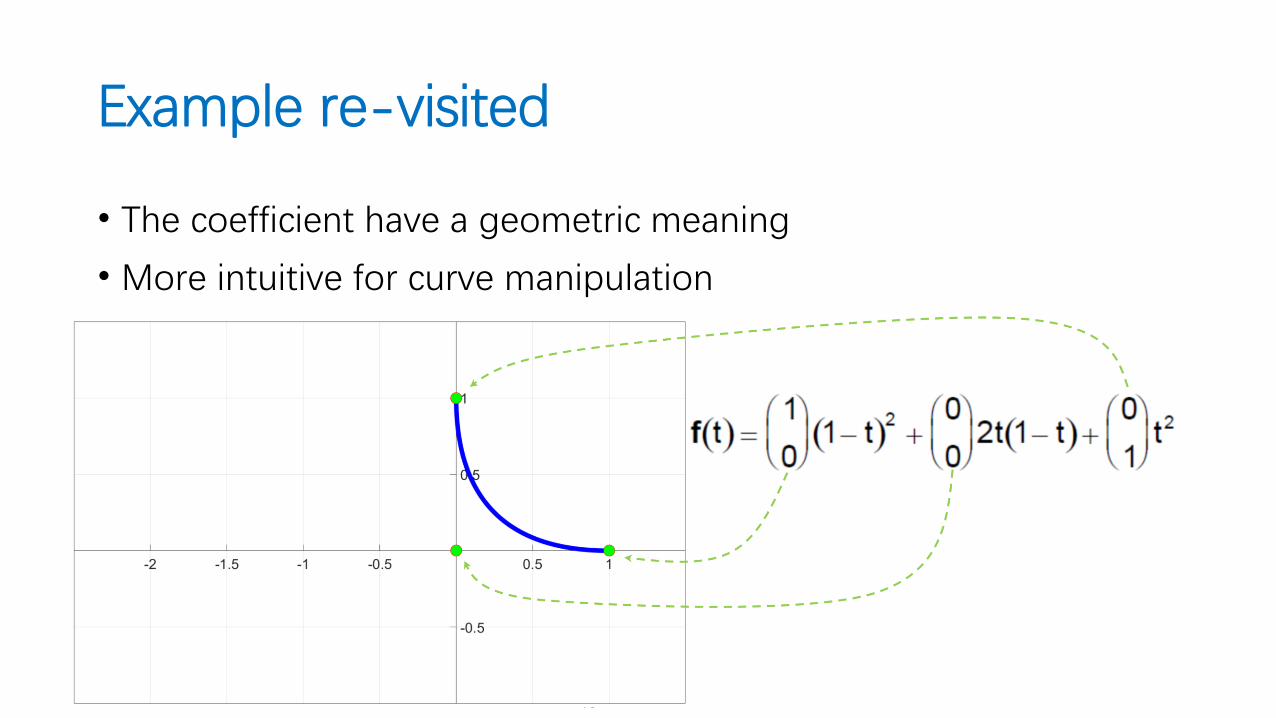
• The coefficient have a geometric meaning

• More intuitive for curve manipulation

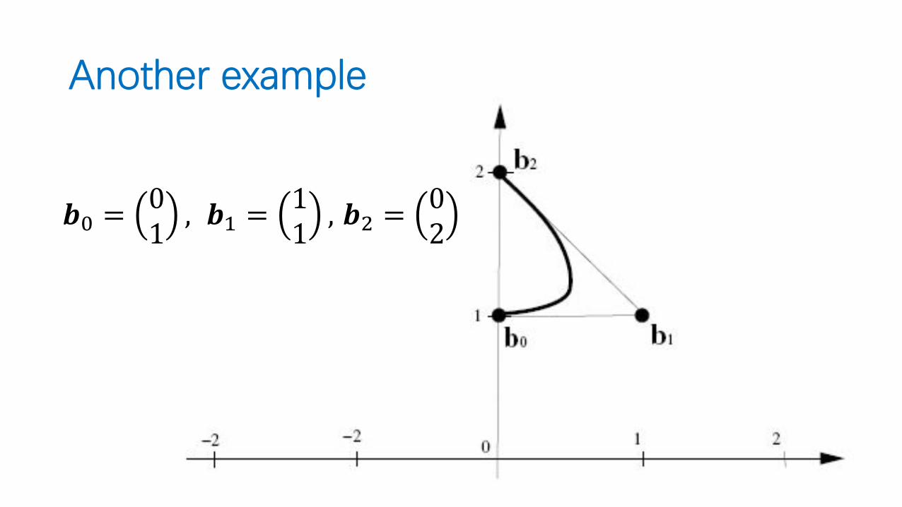
Another example

𝒃0 =01

, 𝒃1 =11

, 𝒃2 =02

Going further

• Cubic approximation

• Given 4 points: 𝒑00 𝑡 = 𝒑0, 𝒑1

0 𝑡 = 𝒑1, 𝒑20 𝑡 = 𝒑2, 𝒑3

0 𝑡 = 𝒑3

• First iteration

• 2nd iteration

• Curve𝒄 𝑡 = 1 − 𝑡 3𝒑0 + 3𝑡 1 − 𝑡 2𝒑1 + 3𝑡2 1 − 𝑡 𝒑2 + 𝑡3𝒑3

𝒑02 = 1 − 𝑡 2𝒑0 + 2𝑡 1 − 𝑡 𝒑1 + 𝑡2𝒑2

𝒑12 = 1 − 𝑡 2𝒑1 + 2𝑡 1 − 𝑡 𝒑2 + 𝑡2𝒑3

𝒑01 = 1 − 𝑡 𝒑0 + 𝑡𝒑1

𝒑11 = 1 − 𝑡 𝒑1 + 𝑡𝒑2

𝒑21 = 1 − 𝑡 𝒑2 + 𝑡𝒑3

Throughout these examples, we just re-invented a primitive version of the de Casteljau algorithm

Now let’s examine it more closely …

De Casteljau algorithm

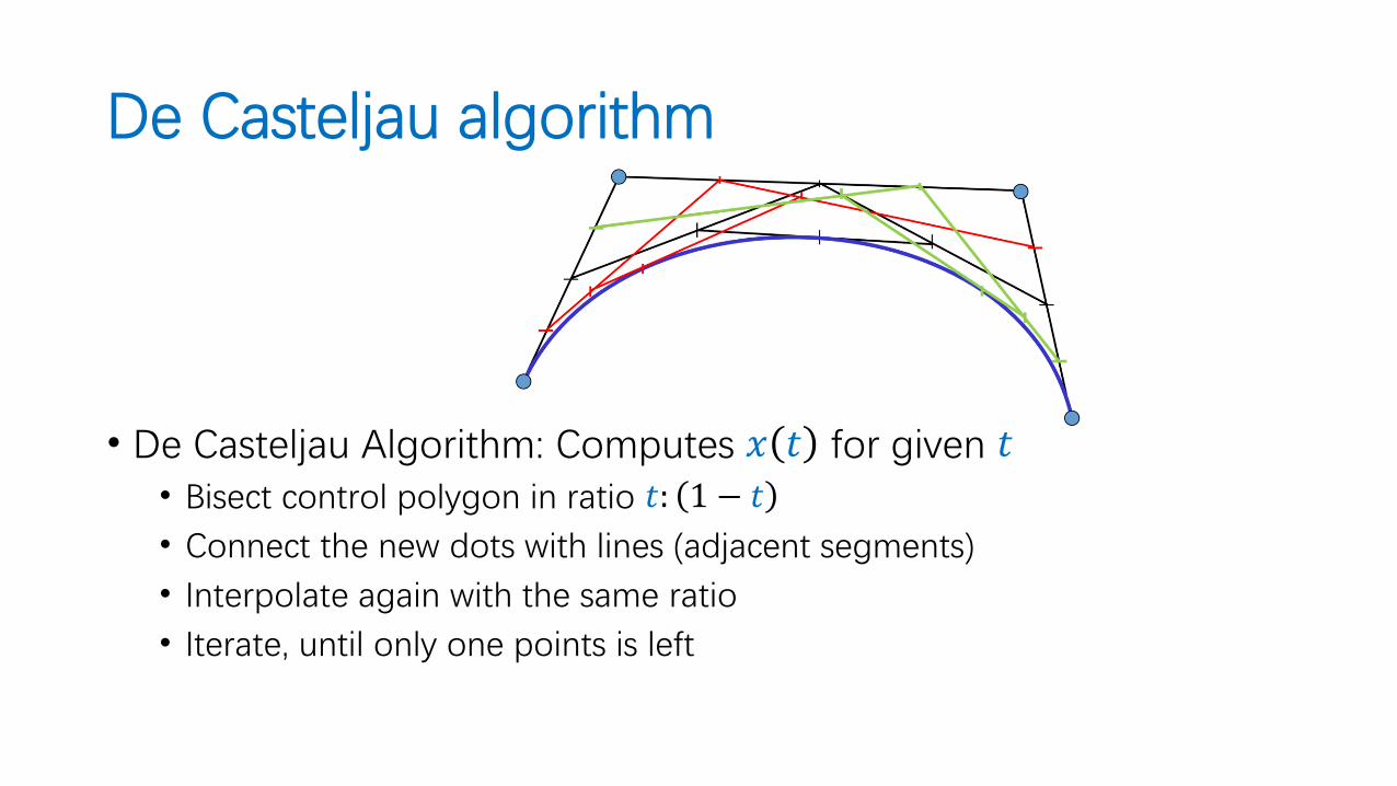
• De Casteljau Algorithm: Computes 𝑥 𝑡 for given 𝑡• Bisect control polygon in ratio 𝑡: 1 − 𝑡

• Connect the new dots with lines (adjacent segments)

• Interpolate again with the same ratio

• Iterate, until only one points is left

















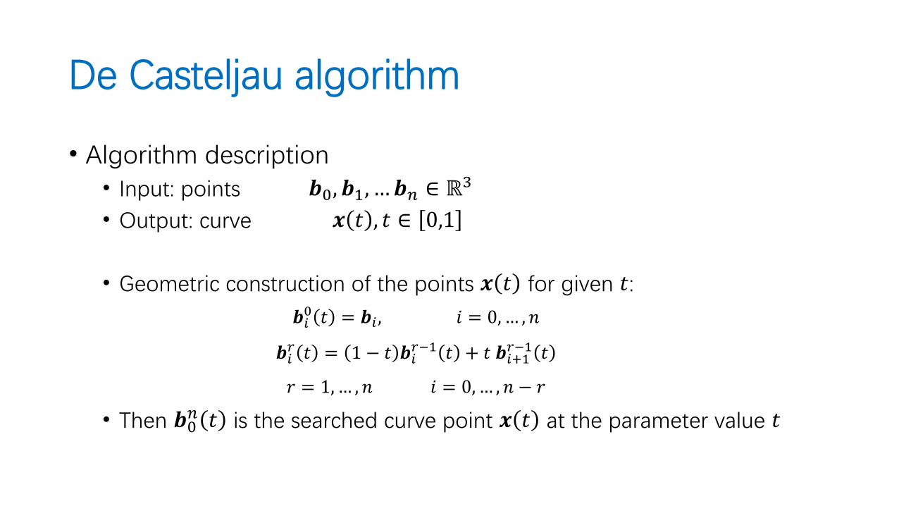
• Algorithm description• Input: points 𝒃0, 𝒃1, …𝒃𝑛 ∈ ℝ3

• Output: curve 𝒙 𝑡 , 𝑡 ∈ 0,1

• Geometric construction of the points 𝒙 𝑡 for given 𝑡:

𝒃𝑖0 𝑡 = 𝒃𝑖 , 𝑖 = 0,… , 𝑛

𝒃𝑖𝑟 𝑡 = 1 − 𝑡 𝒃𝑖

𝑟−1 𝑡 + 𝑡 𝒃𝑖+1𝑟−1 𝑡

𝑟 = 1,… , 𝑛 𝑖 = 0,… , 𝑛 − 𝑟

• Then 𝒃0𝑛 𝑡 is the searched curve point 𝒙 𝑡 at the parameter value 𝑡


• Repeated convex combination of control points

𝒃𝑖𝑟= 1 − 𝑡 𝒃𝑖

𝑟−1 +𝑡𝒃𝑖+1𝑟−1

𝒃00

𝒃10

𝒃20

𝒃30




𝑟−1 +𝑡𝒃𝑖+1𝑟−1

𝒃00

𝒃10

𝒃20

𝒃30

𝑡𝒃0

1

𝒃11

𝒃21

𝑡

𝑡




𝑟−1 +𝑡𝒃𝑖+1𝑟−1

𝒃00

𝒃10

𝒃20

𝒃30

𝑡𝒃0

1

𝒃11

𝒃21

𝑡

𝑡

𝑡

𝑡

𝒃02

𝒃12




𝑟−1 +𝑡𝒃𝑖+1𝑟−1

𝒃00

𝒃10

𝒃20

𝒃30

𝑡𝒃0

1

𝒃11

𝒃21

𝑡

𝑡

𝑡

𝑡

𝒃02

𝒃12 𝑡 𝒃0

3= 𝑥(𝑡)

De Casteljau scheme


• The intermediate coefficients 𝒃𝑖𝑟 𝑡 can be written in a triangular matrix: the

de Casteljau scheme:

• 𝒃0 = 𝒃00

• 𝒃1 = 𝒃10 𝒃0

1

• 𝒃2 = 𝒃20 𝒃1

1 𝒃02

• 𝒃3 = 𝒃30 𝒃2

1 𝒃12 𝒃0

3

• ……………………

• 𝒃𝑛−1 = 𝒃𝑛−10 𝒃𝑛−2

1 … 𝒃0𝑛−1

• 𝒃𝑛 = 𝒃𝑛0 𝒃𝑛−1

1 … 𝒃1𝑛−1 𝒃0

𝑛 = 𝑥 𝑡


• Algorithm:

• for r=1..n

• for i=0..n-r

• 𝒃𝑖𝑟= 1 − 𝑡 𝒃𝑖

𝑟−1+ 𝑡 𝒃𝑖+1

𝑟−1

• end

• end

• return 𝒃0𝑛

The whole algorithm consists only of repeated linear interpolations.

De Casteljau algorithm: Properties

• The polygon consisting of the points 𝒃𝟎, … , 𝒃𝒏 is called Bézier polygon(control polygon)

• The points 𝒃𝒊 are called Bézier points (control points)

• The curve defined by the Bézier points 𝒃𝟎, … , 𝒃𝒏 and the de Casteljau algorithm is called Bézier curve

• The de Casteljau algorithm is numerically stable, since only convex combinations are applied.

• Complexity of the de Casteljau algorithm• 𝑂 𝑛2 time• 𝑂 𝑛 memory• with 𝑛 being the number of Bézier points


• Properties of Bézier curves:• Given: Bézier points 𝒃0, … , 𝒃𝑛

Bézier curve 𝒙 𝑡

• Bézier curve is polynomial curve of degree 𝑛

• End points interpolation: 𝒙 0 = 𝒃0, 𝒙 1 = 𝒃𝑛. The remaining Bézierpoints are only approximated in general

• Convex hull property:

Bézier curve is completely inside the convex hull of its Bézier polygon


• Variation diminishing• No line intersects the Bézier curve more often than its Bézier polygon

• Influence of Bézier points: global but pseudo-local• Global: moving a Bézier points changes the whole curve progression

• Pseudo-local: 𝒃𝑖 has its maximal influence on 𝑥 𝑡 at 𝑡 =𝑖

𝑛

• Affine invariance:• Bézier curve and Bézier polygon are invariant under affine

transformations

• Invariance under affine parameter transformations


• Symmetry• The following two Bézier curves coincide, they are only traversed in

opposite directions:

𝒙 𝑡 = 𝒃0, … , 𝒃𝑛 𝒙′ 𝑡 = 𝒃𝑛, … 𝒃0

• Linear Precision:• Bézier curve is line segment, if 𝒃0, … , 𝒃𝑛 are colinear

• Invariance under barycentric combinations

Recap

de Casteljau algorithm

Bézier CurvesTowards a polynomial description

Bézier CurvesTowards a polynomial description

𝑥 𝑡 =

𝑖=0

𝑛

𝐵𝑖𝑛 𝑡 ⋅ 𝑏𝑖

Polynomial description of Bézier curves

• The same problem as before:• Given: 𝑛 + 1 control points 𝒃0, … , 𝒃𝑛• Wanted: Bézier curve 𝒙 𝑡 with 𝑡 ∈ 0,1

• Now with an algebraic approach using basis functions

Desirable Properties

• Useful requirements for a basis:• Well behaved curve

• Smooth basis functions




• Local control (or at least semi-local)• Basis functions with compact support




• Local control (or at least semi-local)• Basis functions with compact support

• Affine invariance:• Appling an affine map 𝒙 → 𝐴𝒙 + 𝑏 on

• Control points

• Curve

Should have the same effect

• In particular: rotation, translation

• Otherwise: interactive curve editing very difficult


• Useful requirements for a basis:• Convex hull property:

• The curve lays within the convex hull of its control points

• Avoids at least too weird oscillations

• Advantages• Computational advantages (recursive intersection tests)

• More predictable behavior

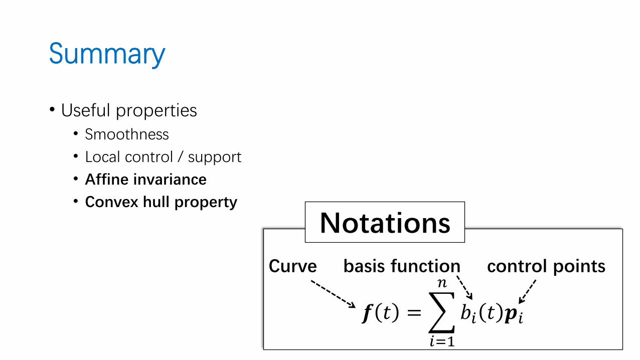
Summary

• Useful properties• Smoothness

• Local control / support

• Affine invariance

• Convex hull property

Curve basis function control points

𝒇 𝑡 =

𝑖=1

𝑛

𝑏𝑖 𝑡 𝒑𝑖

Notations

Affine Invariance

• Affine map: 𝒙 → 𝐴𝒙 + 𝒃

• Part I: Linear invariance – we get this automatically

• Linear approach: 𝒇 𝑡 = σ𝑖=1𝑛 𝑏𝑖 𝑡 𝒑𝑖 = σ𝑖=1

𝑛 𝑏𝑖 𝑡

𝑝𝑖𝑥

𝑝𝑖𝑦

𝑝𝑖𝑧

• Therefore: 𝐴 𝒇 𝑡 = 𝐴 σ𝑖=1𝑛 𝑏𝑖 𝑡 𝒑𝑖 = σ𝑖=1

𝑛 𝑏𝑖 𝑡 𝐴𝒑𝑖

Affine Invariance

• Affine Invariance:• Affine map: 𝒙 → 𝐴𝒙 + 𝒃

• Part II: Translational invariance

𝑖=1

𝑛

𝑏𝑖 𝑡 𝒑𝑖 + 𝒃 =

𝑖=1

𝑛

𝑏𝑖 𝑡 𝒑𝑖 +

𝑖=1

𝑛

𝑏𝑖 𝑡 𝒃 = 𝒇 𝑡 +

𝑖=1

𝑛

𝑏𝑖 𝑡 𝒃

• For translational invariance, the sum of the basis functions must be one everywhere (for all parameter values 𝑡 that are used).

• This is called “partition of unity property”

• The 𝑏𝑖’s form an “affine combination” of the control points 𝒑𝑖• This is very important for modeling

Convex Hull Property

• Convex combinations:• A convex combination of a set of points 𝒑1, … , 𝒑𝑛 is any point of the form:

σ𝑖=1𝑛 𝜆𝑖𝒑𝒊 with σ𝑖=1

𝑛 𝜆𝑖 = 1 and ∀𝑖 = 1…𝑛: 0 ≤ 𝜆𝑖 ≤ 1

• (Remark: 𝜆𝑖 ≤ 1 is redundant)

• The set of all admissible convex combinations forms the convex hull of the point set• Easy to see (exercise): The convex hull is the smallest set that contains all points

𝒑1, … , 𝒑𝑛 and every complete straight line between two elements of the set


• Accordingly:• If we have this property∀𝑡 ∈ Ω:σ𝑖=1

𝑛 𝑏𝑖 𝑡 = 1 and ∀𝑡 ∈ Ω, ∀𝑖: 𝑏𝑖 𝑡 ≥ 0

the constructed curves / surfaces will be:• Affine invariant (translations, linear maps)

• Be restricted to the convex hull of the control points

• Corollary: Curves will have linear precision• All control points lie on a straight line

⇒ Curve is a straight line segment

• Surfaces with planar control points will be flat, too


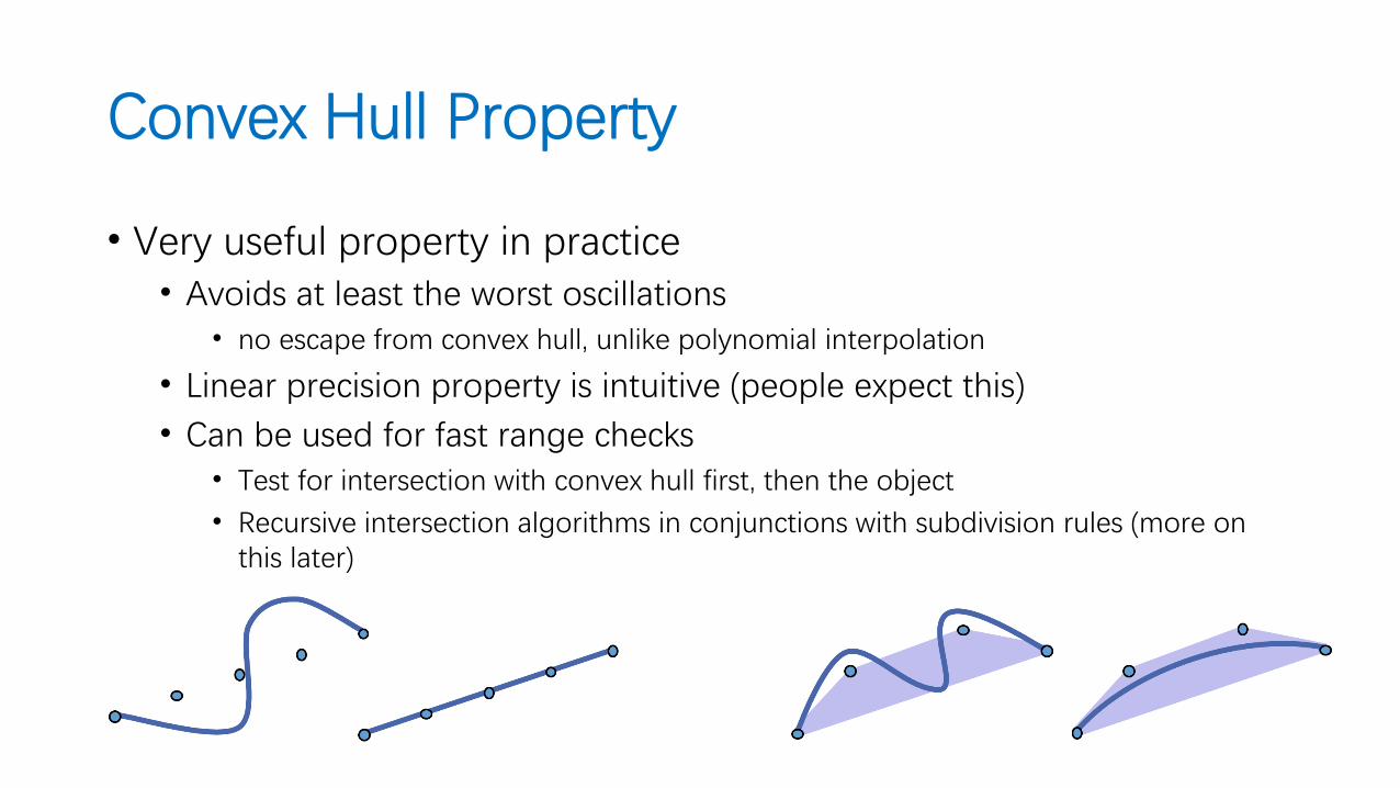
• Very useful property in practice• Avoids at least the worst oscillations

• no escape from convex hull, unlike polynomial interpolation

• Linear precision property is intuitive (people expect this)

• Can be used for fast range checks• Test for intersection with convex hull first, then the object

• Recursive intersection algorithms in conjunctions with subdivision rules (more on this later)

Polynomial description of Bézier curves

• The same problem as before:• Given: 𝑛 + 1 control points 𝒃0, … , 𝒃𝑛• Wanted: Bézier curve 𝑥 𝑡 with 𝑡 ∈ 0,1

• Now with an algebraic approach using basis functions

• Need to define 𝑛 + 1 basis functions• Such that this describes a Bézier curve:

𝐵0𝑛 𝑡 , … , 𝐵𝑛

𝑛 𝑡 over 0,1

𝒙 𝑡 =

𝑖=0

𝑛

𝐵𝑖𝑛 𝑡 ⋅ 𝒃𝑖

Bernstein Basis

• Let’s examine the Bernstein basis: 𝐵 = {𝐵0𝑛, 𝐵1

𝑛, … , 𝐵𝑛

𝑛}

• Bernstein basis of degree 𝑛:

𝐵𝑖𝑛

𝑡 =𝑛𝑖𝑡𝑖 1 − 𝑡 𝑛−𝑖 = 𝐵𝑖−th basis function

degree

where the binomial coefficients are given by:

𝑛𝑖

= ቐ

𝑛!

𝑛 − 𝑖 ! 𝑖!for 0 ≤ 𝑖 ≤ 𝑛

0 otherwise

Binomial Coefficients and Theorem

𝑥 + 𝑦 𝑛 =

𝑖=0

𝑛𝑛𝑖

𝑥𝑖𝑦𝑛−𝑖

𝑛𝑖

+𝑛

𝑖 + 1=

𝑛 + 1𝑖 + 1

Examples: The first few

• The first three Bernstein bases:

• 𝐵00≔ 1

• 𝐵01≔ 1− 𝑡 𝐵1

1≔ 𝑡

• 𝐵02≔ 1− 𝑡 2 𝐵1

2≔ 2𝑡 1 − 𝑡 𝐵2

2≔ 𝑡2

• 𝐵03≔ 1− 𝑡 3 𝐵1

3≔ 3𝑡 1 − 𝑡 2 𝐵2

3≔ 3𝑡2 1 − 𝑡 𝐵3

3≔ 𝑡3

𝐵𝑖𝑛

𝑡 =𝑛𝑖

𝑡𝑖 1 − 𝑡 𝑛−𝑖

Examples: The first few

• 𝐵03≔ 1− 𝑡 3

• 𝐵13≔ 3𝑡 1 − 𝑡 2

• 𝐵23≔ 3𝑡2 1 − 𝑡

• 𝐵33≔ 𝑡3

𝐵𝑖𝑛

𝑡 =𝑛𝑖


𝐵00≔ 1

𝐵01≔ 1− 𝑡

𝐵11≔ 𝑡

𝐵02≔ 1− 𝑡 2

𝐵12≔ 2𝑡 1 − 𝑡

𝐵22≔ 𝑡2

Bernstein Basis

• Bézier curves use the Bernstein basis: 𝐵 = 𝐵0𝑛, 𝐵1

𝑛, … , 𝐵𝑛

𝑛

• Bernstein basis of degree 𝑛:

𝐵𝑖𝑛

𝑡 =𝑛𝑖𝑡𝑖 1 − 𝑡 𝑛−𝑖 = 𝐵𝑖−th basis function

degree

Bernstein Basis

• What about the desired properties?• Smoothness




Bernstein Basis: Properties

• 𝐵 = 𝐵0𝑛, 𝐵1

𝑛, … , 𝐵𝑛

𝑛 , 𝐵𝑖𝑛

𝑡 =𝑛𝑖


• Basis for polynomials of degree 𝑛

• Each basis function 𝐵𝑖𝑛 has its maximum at 𝑡 =

𝑖

𝑛

Smoothness

Local control (semi-local)


• 𝐵 = 𝐵0𝑛, 𝐵1

𝑛, … , 𝐵𝑛

𝑛 , 𝐵𝑖𝑛

𝑡 =𝑛𝑖


• Partition of unity (binomial theorem)1 = 1 − 𝑡 + 𝑡

𝑖=0

𝑛

𝐵𝑖𝑛

𝑡 = 𝑡 + 1 − 𝑡𝑛= 1

Affine invariance Convex hull property

What about the desired properties?

• Smoothness




YesTo some extentYesYes


• 𝐵 = 𝐵0𝑛, 𝐵1

𝑛, … , 𝐵𝑛

𝑛 , 𝐵𝑖𝑛

𝑡 =𝑛𝑖


• Recursive computation

𝐵𝑖𝑛 𝑡 ≔ 1 − 𝑡 𝐵𝑖

𝑛−1𝑡 + 𝑡𝐵𝑖−1

𝑛−11 − 𝑡

with 𝐵00 𝑡 = 1, 𝐵𝑖

𝑛 𝑡 = 0 for 𝑖 ∉ 0…𝑛

• Symmetry𝐵𝑖𝑛 𝑡 = 𝐵𝑛−𝑖

𝑛 1 − 𝑡

• Non-negativity: 𝐵𝑖𝑛

𝑡 ≥ 0 for 𝑡 ∈ [0. . 1]

𝑛 − 1𝑖

+𝑛 − 1𝑖 − 1

=𝑛𝑖


• 𝐵 = 𝐵0𝑛, 𝐵1

𝑛, … , 𝐵𝑛

𝑛 , 𝐵𝑖𝑛

𝑡 =𝑛𝑖


• Non-negativity II

𝐵𝑖𝑛 𝑡 > 0 for 0 < 𝑡 < 1

𝐵0𝑛 0 = 1, 𝐵1

𝑛 0 = ⋯ = 𝐵𝑛𝑛 0 = 0

𝐵0𝑛 1 = ⋯ = 𝐵𝑛−1

𝑛 1 = 0, 𝐵𝑛𝑛 1 = 1

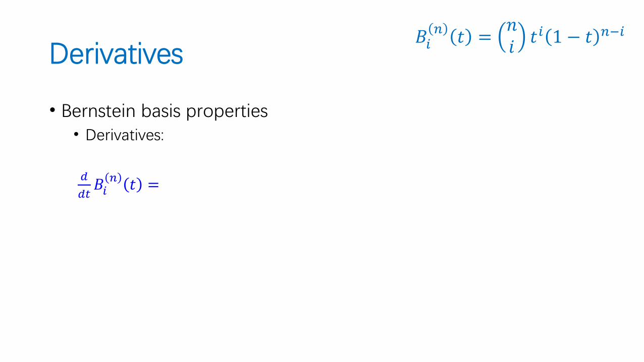
Derivatives𝐵𝑖

𝑛𝑡 =

𝑛𝑖


• Bernstein basis properties• Derivatives:

𝑑

𝑑𝑡𝐵𝑖

𝑛𝑡 =

Derivatives𝐵𝑖

𝑛𝑡 =

𝑛𝑖



𝑑

𝑑𝑡𝐵𝑖

𝑛𝑡 =

𝑛𝑖

𝑖𝑡 𝑖−1 1 − 𝑡 𝑛−𝑖 − 𝑛 − 𝑖 𝑡𝑖 1 − 𝑡 𝑛−𝑖−1

=𝑛!

𝑛 − 𝑖 ! 𝑖!𝑖𝑡 𝑖−1 1 − 𝑡 𝑛−𝑖 −

𝑛!

𝑛 − 𝑖 ! 𝑖!𝑛 − 𝑖 𝑡𝑖 1 − 𝑡 𝑛−𝑖−1

= 𝑛𝑛 − 1𝑖 − 1

𝑡 𝑖−1 1 − 𝑡 𝑛−𝑖 −𝑛 − 1𝑖

𝑡𝑖 1 − 𝑡 𝑛−𝑖−1

= 𝑛 𝐵𝑖−1𝑛−1

𝑡 − 𝐵𝑖𝑛−1

𝑡

(Notation: {𝒌} = 𝒌 if 𝒌 > 𝟎, zero otherwise)

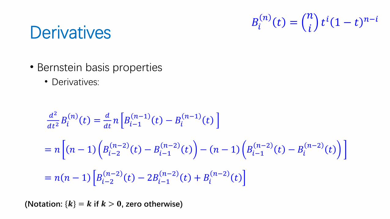
Derivatives𝐵𝑖

𝑛𝑡 =

𝑛𝑖



𝑑2

𝑑𝑡2𝐵𝑖

𝑛𝑡 =

𝑑

𝑑𝑡𝑛 𝐵𝑖−1

𝑛−1𝑡 − 𝐵𝑖

𝑛−1𝑡

= 𝑛 𝑛 − 1 𝐵𝑖−2𝑛−2

𝑡 − 𝐵𝑖−1𝑛−2

𝑡 − 𝑛 − 1 𝐵𝑖−1𝑛−2


𝑡

= 𝑛 𝑛 − 1 𝐵𝑖−2𝑛−2

𝑡 − 2𝐵𝑖−1𝑛−2

𝑡 + 𝐵𝑖𝑛−2

𝑡

(Notation: {𝒌} = 𝒌 if 𝒌 > 𝟎, zero otherwise)

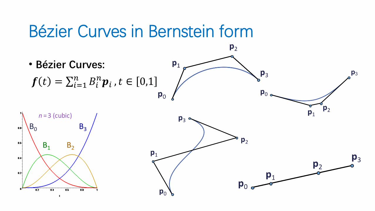
Bézier Curves in Bernstein form

• Bézier Curves:

𝒇 𝑡 = σ𝑖=1𝑛 𝐵𝑖

𝑛𝒑𝑖 , 𝑡 ∈ 0,1


• Bézier Curves:


𝑛𝒑𝑖 , 𝑡 ∈ 0,1


• Bézier Curves:


𝑛𝒑𝑖 , 𝑡 ∈ 0,1


• Bézier Curves:


𝑛𝒑𝑖 , 𝑡 ∈ 0,1


• Bézier Curves, also in 3D


𝑛𝒑𝑖 , 𝑡 ∈ 0,1


• Bézier curves:• Curves: 𝒇 𝑡 = σ𝑖=1

𝑛 𝐵𝑖𝑛𝒑𝑖

• Considering the interval 𝑡 ∈ 0. . 1

• Properties as discussed before:• Affine invariant

• Curves contained in the convex hull

• Influence of control points

Moving along the curve with index 𝑖

Largest influence at 𝑡 =𝑖

𝑛

Single curve segments: no full local control

Bézier Curve Properties: another look at derivatives

• Given: 𝒑0, … , 𝒑𝑛, 𝒇 𝑡 = σ𝑖=0𝑛 𝐵𝑖

𝑛 𝑡 𝒑𝑖

• Then: 𝒇′ 𝑡 = 𝑛σ𝑖=0𝑛−1𝐵𝑖

𝑛−1 𝑡 𝒑𝑖+1 − 𝒑𝑖

• Proof: 𝒇′ 𝑡 = σ𝑖=0𝑛 𝑑

𝑑𝑡𝐵𝑖𝑛 𝑡 𝒑𝑖 = 𝑛σ𝑖=0

𝑛 𝐵𝑖−1𝑛−1 𝑡 − 𝐵𝑖

𝑛−1 𝑡 𝒑𝑖

= 𝑛

𝑖=0

𝑛

𝐵𝑖−1𝑛−1 𝑡 𝒑𝑖 − 𝑛

𝑖=0

𝑛

𝐵𝑖𝑛−1 𝑡 𝒑𝑖

= 𝑛

𝑖=−1

𝑛−1

𝐵𝑖𝑛−1 𝑡 𝒑𝑖+1 − 𝑛

𝑖=0

𝑛

𝐵𝑖𝑛−1 𝑡 𝒑𝑖 = 𝑛

𝑖=0

𝑛−1

𝐵𝑖𝑛−1 𝑡 𝒑𝑖+1 − 𝑛

𝑖=0

𝑛−1

𝐵𝑖𝑛−1 𝑡 𝒑𝑖

= 𝑛

𝑖=0

𝑛−1

𝐵𝑖𝑛−1 𝑡 𝒑𝑖+1 − 𝒑𝑖

Index change

Bézier Curve Properties

• Higher order derivatives:

𝑓 𝑟 𝑡 =𝑛!

𝑛 − 𝑟 !⋅

𝑖=0

𝑛−𝑟

𝐵𝑖𝑛−𝑟 𝑡 ⋅ Δ𝑟𝒑𝑖


• Imporant for continuous concatenation:• Function value at 0,1 :

𝒇 𝑡 =

𝑖=0

𝑛−1𝑛𝑖

𝑡𝑖 1 − 𝑡 𝑛−𝑖𝒑𝑖

⇒ 𝒇 0 = 𝒑0𝒇 1 = 𝒑1

• First derivative vector at 0,1

• Second derivative vector at 0,1


First derivative vector at 0,1𝑑

𝑑𝑡𝒇 𝑡 =


First derivative vector at 0,1

𝑑

𝑑𝑡𝒇 𝑡 = 𝑛

𝑖=0

𝑛−1

𝐵𝑖−1𝑛−1


𝑡 𝒑𝑖


First derivative vector at 0,1

𝑑

𝑑𝑡𝒇 𝑡 = 𝑛

𝑖=0

𝑛−1

𝐵𝑖−1𝑛−1


𝑡 𝒑𝑖

= 𝑛 ቀ

ቁ

−𝐵0𝑛−1

𝑡 𝒑0 + 𝐵0𝑛−1

𝑡 − 𝐵1𝑛−1

𝑡 𝒑1 +⋯

+ 𝐵𝑛−2𝑛−1

𝑡 − 𝐵𝑛−1𝑛−1

𝑡 𝒑𝑛−1 + 𝐵𝑛−1𝑛−1

𝑡 𝒑𝑛

𝑑

𝑑𝑡𝒇 0 = 𝑛 𝒑1 − 𝒑0

𝑑

𝑑𝑡𝒇 1 = 𝑛 𝒑𝑛 − 𝒑𝑛−1


• Imporant for continuous concatenation:• Function value at 0,1 :

𝒇 0 = 𝒑0𝒇 1 = 𝒑1

• First derivative vector at 0,1𝒇′ 0 = 𝑛 𝒑1 − 𝒑0𝒇′ 1 = 𝑛 𝒑𝑛 − 𝒑𝑛−1

• Second derivative vector at 0,1𝒇′′ 0 = 𝑛 𝑛 − 1 𝒑2 − 𝟐𝒑1 + 𝒑0

𝒇′′ 1 = 𝑛 𝑛 − 1 𝒑𝑛 − 2𝒑𝑛−1 + 𝒑𝑛−2

Documents

计算机辅助几何设计 2021秋学期 Bézier Curves