Munich Personal RePEc Archive

A Theory of Continuum Economies with

Idiosyncratic Shocks and Random

Matchings

Karavaev, Andrei

Pennsylvania State University

25 February 2008

Online at https://mpra.ub.uni-muenchen.de/7445/

MPRA Paper No. 7445, posted 05 Mar 2008 07:53 UTC

A Theory of Continuum Economies with

Idiosyncratic Shocks and Random Matchings1

Andrei Karavaev2

This version: February 2008

“Entities should not be multiplied beyond necessity.”

Occam’s razor

Many economic models use a continuum of negligible agents to avoid con-

sidering one person’s effect on aggregate characteristics of the economy.

Along with a continuum of agents, these models often incorporate a se-

quence of independent shocks and random matchings. Despite frequent use

of such models, there are still unsolved questions about their mathemat-

ical justification. In this paper we construct a discrete time framework,

in which major desirable properties of idiosyncratic shocks and random

matchings hold. In this framework the agent space constitutes a proba-

bility space, and the probability distribution for each agent is replaced by

the population distribution. Unlike previous authors, we question the as-

sumption of known identity — the location on the agent space. We assume

that the agents only know their previous history — what had happened to

them before, — but not their identity.

The construction justifies the use of numerous dynamic models of id-

iosyncratic shocks and random matchings.

Key Words and Phrases: random matching, idiosyncratic shocks, the Law of Large

Numbers, aggregate uncertainty, mixing.

JEL Classification Numbers: C78, D83, E00.

1I am indebted to my advisor Kalyan Chatterjee who guided this work. This paper would not be

possible without his encouragement. I also thank Edward Green, James Jordan, and Sophie Bade for

their helpful comments.2Department of Economics, 608 Kern Graduate Building, The Pennsylvania State University, Univer-

sity Park, PA 16802. E-mail: akaravae@psu.edu.

1

2

1. Introduction

The Problem

A large number of economic models consider an uncountable number of negligible agents

who experience idiosyncratic shocks and randomly meet each other. Some examples

of such models are given by Aliprantis et al. [2], Alos-Ferrer [4], and Boylan [7]. The

assumptions in these models are made in the spirit of the Law of Large Numbers. For

example, the mixing property assumption is often used, which states that the fraction of

the agents from one set who are matched with the agents from another set equals the

measure of the second set.3 Until recently there was no formal mathematical evidence

that such models exist. Moreover, some economists pointed out serious contradictions

among the standard assumptions used.

The existence of many economic models with both idiosyncratic shocks and random

matchings4 makes it impossible to discuss all the discrepancies that arise. Therefore, we

give here only two most famous examples of contradictions in the standard assumptions.

One of the most famous contradictions was described by Judd [19].5 It has been as-

sumed that the average of a continuum of independent and identically distributed random

variables (idiosyncratic shocks) is nonrandom (no aggregate uncertainty property). Judd

shows that the nonrandomness of the average neither contradicts nor follows from the

independence and identical distribution of the shocks. Moreover, Judd proves that if the

population is represented by the unit interval with the Borel σ-algebra, then most of the

shock realizations on the agent space are not measurable and therefore the average shock

cannot be calculated. Feldman and Gills [12] notice that measurable functions on the unit

interval are in some sense “almost continuous.” However, “almost continuity” of shock

3Shi [21] describes the following matching process with the mixing assumption: “... the distribution

of different types of matches for each household is almost surely nonrandom, although each member in

the household is uncertain about the kind of agent he will meet.”4The word “meeting” will be used with respect to one agent. The one-time process of all the agents

of the population being paired up with each other will be called “matching.”5This and the random matching example will be considered in details in Section 3.3. “Standard Model

Inconsistencies.”

3

realizations contradicts the independence of shocks for different agents implied by the

idiosyncratic nature of the shocks.6

A second contradiction is about random matching assumptions. It was described by

McLennan and Sonnenschein [20] in footnote 4. Using Proposition 1 from Feldman and

Gilles [12], the authors show that a measure preserving matching can not be mixing. The

source of the contradiction is also measurability: the agents who are “close” to each other

on the agent space should be paired up with the agents who are also “close” to each

other,7 which contradicts the randomness of the meetings.

There exist several solutions to the idiosyncratic shocks problem (see the literature

review for the details.) There are also several papers dealing with the random matching

problem. At the same time, to our knowledge, there is no paper dealing with both

idiosyncratic shocks and random matching. Furthermore, no existing paper completely

justifies the mixing property of a random matching simultaneously for all the measurable

subsets of the agents, which is the cornerstone of many economic models. In this paper

we build a mathematically valid discrete time model of idiosyncratic shocks and random

matchings, which resolves the conflicting issues.

The Causes of the Problem

All the contradictions among the standard assumptions stem from an uncountable

number of the agents. The very idea of considering a non-atomic agent space comes from

the convenient properties of a finite but large population of agents. For example, because

of the Law of Large Numbers, in a large but finite population the average shock is close

to the average shock for each agent. Thus, by using a continuum of agents, one wants

to achieve two important goals. The first one is to have negligible agents who have no

influence on the aggregate characteristics of the economy. The second goal is to have an

analogue of the Law of Large Numbers with respect to shocks and meetings.8

6Measurable functions on the unit interval have a good approximation by the continuous functions

(Luzin’s theorem); Al-Najjar [1] in Theorem 8 shows that “a typical realization of an i.i.d. process can

not be approximated by a continuous function.”7As Alos-Ferrer [4] puts it, “the very concept of matching destroys the most basic independence

aspirations.”8As Gilboa and Matsui [15] wrote, “...there are uncountably many agents of various types, each of

which has no effect whatsoever on the aggregate behavior, thus eliminating strategic considerations which

4

A replacement of a large but finite agent space with an uncountable space of negligible

agents has several hidden problems arising from significant differences in the structures of

these spaces. For a finite space, the measure comes naturally (the counting measure) and

in the unique way. One-to-one matching automatically guarantees the measure preserv-

ing property. The natural discrete σ-algebra consists of all the subsets, making all the

functions measurable. For an uncountable space, the choice of the measure is ambiguous.

Additional assumptions should be made to guarantee the measure preserving property of

the matching. Measurability seriously restricts the set of functions and matchings.9

The Main Idea

The existing models assume that the agents know their identity — the exact location

on the agent space. For example, the requirement that the shocks are independent for

different agents is only necessary if the agents know who they are. Because of the known

identity, the standard setup requires the space of the states of the world, which allows us to

model the uncertainty the agents face about their future shocks and meetings. Therefore,

two different spaces are needed: the space of the agents and the space of the states of the

world. The shocks and matchings are defined on their product.

However, in many economic models the knowledge of identity is excessive and has no

influence on the results. What the models really require is that the agents have their own

attributes, like type, initial endowment, etc.10 Another requirement is that the agents

perceive their future as random.11 With these assumptions, the agents use strategies

extend beyond a specific encounter.” Alos-Ferrer [5] notices that “...oftentimes, agents have to be modeled

as being negligible.” Alos-Ferrer [4] also mentions convenience in using a continuum of agents because of

analytical simplicity and anonymity properties.9Al-Najjar [1] discusses the measurability problem in Section 4. As he notices, this problem emerges

because the agents who are ex ante similar have to have independent shocks ex post.10Kandori [19] describes the following rules: “1. A label is attached to each agent. 2. Before executing

trade each agent observes his and his partner’s label. 3. A player and his partner’s actions and labels

today determine their labels tomorrow.”11Gale [14] requires the following form of randomness: “the probability of an active agent meeting an

agent whose history <belongs to some set> is independent of the first agent’s history.”

5

which depend only on the history and some initial attributes.12 The idea of such history-

dependent strategies implies that the agents do not know their identities; otherwise they

would include it in their strategies.

Based on the idea of unknown identity, we suggest to simplify the setup and consider

only one space — the agent space, which also serves as the probability space. With this

approach the agents still face some randomness. It does not come from the realization

of the state of the world, but from the unknown identity. Each agent believe that he

was placed randomly (and uniformly) on the agent space. The shocks and meetings are

predetermined.13 However, the agents do not know their identities and therefore perceive

thir shocks and meetings as random. The events help the agents to refine the knowledge

of their identities, but do not resolve it completely. Based on the previous shocks and

meetings, the agents update their beliefs about the future.14

The Results

The main result of the paper (Theorem 2) states that there exists a mathematically

correct dynamic discrete time model of negligible agents with idiosyncratic shocks and

random matchings. The shocks and matchings are measurable. The matchings are mea-

sure preserving. For any agent his shocks and meetings are independent of the past

events. The equivalent of the Law of Large Numbers holds with respect to the σ-algebras

generated by the histories.

Many discrete time economic models with idiosyncratic shocks and random matchings

can be reformulated in the new setup. The model is very flexible. It can incorporate

12Green and Zhou [17] write: “an agent’s strategy is a function of only his own trading history and

initial money holdings...”13This makes the shocks and meetings of different agents to be dependent. This idea is not new; it was

explored in Feldman and Gilles [12] and Alos-Ferrer [5] and [4]. Boylan [7] and Alos-Ferrer [4] showed

that the matching scheme should be dependent on the assignment of types (shocks). However, in these

papers the agents know their identities and therefore this dependence can influence the choice of the

strategies.14This approach is similar to the Kolmogorov definition of the probability space. Namely, in Kol-

mogorov’s definition random variables are some measurable functions on the probability space Ω. The

realization ω ∈ Ω is not known to the observer(s); initially it is chosen at random. The observers(s) can

update the belief about ω based on the events.

6

some additional characteristics of the agents, such as type, product consumed, etc. It also

permits shocks and matchings that depend on the agents’ histories or other characteristics.

Plan of the Paper

The rest of the paper is organized as follows. Section 2 contains the literature review.

Section 3 discusses the standard assumptions used in economic models and shows the

problems arising from the use of these assumptions. In section 4, we give the formal

definition and prove the existence of idiosyncratic shocks and random matchings. Section

5 concludes. All the proofs are given in the Appendix.

2. Literature Review

All the related literature naturally falls into two different categories: idiosyncratic

shocks and random matchings.

2.1. Idiosyncratic Shocks

Judd [19] and Feldman and Gilles [12] were among the first economists to notice that

for the unit interval of agents with the Borel σ-algebra and Lebesgue measure either the

shocks are not measurable across the population, or the equivalent of the Law of Large

Numbers does not hold.15 Several remedies to the problem of idiosyncratic shocks were

offered by Judd, Feldman and Gilles, and other economists.

Judd [19] solves the problem of idiosyncratic shocks on the whole agent space. The idea

is to build an extension of the agent space so that the Law of Large Numbers is satisfied.

The author notices that the extension is not unique, and for other extensions the Law

of Large Numbers might fail.16 Feldman and Gilles [12] suggest relaxing the assumption

of shocks independence or considering finite or countably infinite approximations of the

15Judd proves that the measure of the realizations for which the sample distribution function on the

unit interval of agents does not exist has inner measure zero and outer measure one. He also shows that

there is an extension of the whole space for which the Law of Large Numbers holds for the whole agent

space. Feldman and Gilles show that there is no extension for which “a law of large numbers is valid

simultaneously for all members of σ-algebra.” As Sun [22] mentions, Doob [9] noticed long ago that “the

sample functions of such a process are usually too irregular to be useful.”16Several other authors, including Green [16] and Alos-Ferrer [5], mention non-uniqueness of the exten-

sion. From our point of view, non-uniqueness does not really constitute a problem. The goal is to find a

7

agent space. A countably infinite population provides an appropriate idealization of a

large economy. The authors show that there exists a density charge on the agent space

such that the Law of Large Numbers is satisfied. Al-Najjar [1] also considers a sequence

of finite but increasingly large economies. The continuum-like laws, including the Law of

Large Numbers for any subinterval of the [0, 1] set of agents, hold in important aspects,

although the measure is not countably additive and the integral might not coincide with

the Lebesgue integral.

Developing the idea of dependent shocks, Alos-Ferrer [5] suggests to consider a pop-

ulation extension. To illustrate the population extension, consider a randomly rotated

circumference of agents which is naturally mapped onto the original circumference. The

shock (chosen from a finite set) of an agent is the one that was originally at the point of

the circumference before the rotation. The shocks in this model are not independent, but

the Law of Large Numbers holds on the whole space.

Instead of the Lebesque integral, Uhlig [23] uses the Pettis integral to calculate the

average shock, which captures the idea of a countable normalized sum of shocks. On the

unit interval of agents the Pettis integral is equivalent to the L2-Riemann integral. If

the shocks are pairwise uncorrelated and have the same mean and uniformly bounded

variances, the Pettis integral exists. Uhlig shows that the Law of Large Numbers holds:

the Pettis integral on any measurable subset of the agents is almost everywhere constant.

Green [16] changes the agent space by endowing the unit interval with a σ-algebra

richer then the Borel σ-algebra. He constructs a family of iid variables on this nonatomic

space so that for any subset of the population with a positive measure the Law of Large

Numbers holds almost surely. Sun [22] uses hyperfinite Loeb spaces to demonstrate the

same type of no aggregate uncertainty.17 The results on the hyperfinite space can be

routinely translated into large finite populations models.

viable mathematical setup, and the question we want to answer is if we can justify using an uncountable

number of agents.”17Judd [19] suggested using hyperfinite discrete models from nonstandard analysis to solve the problem

of idiosyncratic shocks.

8

2.2. Random Matching

The problems of random matching and idiosyncratic shocks have the same roots. Nev-

ertheless, the random matching problem is more challenging because of the additional

assumptions on the structure of the matching. Several authors suggested their remedies

to the problem, which essentially use the same ideas as the solutions of the idiosyncratic

shocks problem.

Gilboa and Matsui [15] were the first to approach the random matching problem. They

consider a continuous time model with only a few individuals out of a countable popu-

lation meeting at each period of time. Each individual meets someone only once. The

probability measure in the model is finitely additive. The authors satisfy the properties

of no aggregate uncertainty for any measurable set of the agents and randomness of the

meetings. Boylan [7] also considers countably many agents. The Law of Large Numbers

is formulated with respect to a finite set of agent types. The randomness implies that

the type proportions evolve in accordance with the mixing property. The author develops

a matchings scheme in which the mixing property holds, however the matching scheme

can not be independent of the assignment of types. In [8] Boylan discusses the conditions

under which a finite deterministic matching approximates a random matching process

with continuous time as the population grows to infinity.

Alos-Ferrer [4] considers a random matching of a continuum of agents. He uses the

tool of population extension developed in Alos-Ferrer [5] and proves the existence of a

random matching satisfying the Law of Large Numbers properties with respect to a finite

set of types. In [6], the author extends the results to several populations. Duffie and

Sun [11] employ the framework of hyperfinite Loeb spaces (see Sun [22] above). The

matching agents are assigned a finite number of types. The authors find an agent space

and a random matching satisfying the following properties: measure preserving, uniform

distribution, and mixing (for any two given sets of the agents the mixing property holds

with probability one). For any two different agents their partners’ types are independent.

The matching scheme is independent in types for any assignment of types. In [10] the

authors study the type distribution evolvement induced by the matchings and random

mutations.

9

Although Aliprantis et al. [2] and [3] do not suggest any solution to the random match-

ing problem, they use a set-theoretical approach to build a foundation for the random

matching models. The basic object they consider is a cluster — several agents meeting at

some period of time. The matching rule consists of non-intersecting k-element clusters.

The stochastic matching rule is defined as a probability measure over all k-clustering

matching rules. Although the authors mainly concentrate on finite-agent models, they

define such general concepts as direct and indirect partners, along with anonymous and

strongly anonymous sequences of k-clustering matching rules.

2.3. Why Further Solution?

Although the papers mentioned partially solve the problems of idiosyncratic shocks and

random mmatchings, no solution guarantees no aggregate uncertainty/mixing property

simultaneously for all the measurable subsets of the agent space (many of them also do

not have other important characteristics, like countably additive measure, anonymous

meetings, Lebesgue integral, independent shocks/meetings, etc.) No paper deals with

both idiosyncratic shocks of a general distribution and random matchings.

Duffie and Sun [11] suggest a random matching in which the properties do not hold

almost surely for all the subsets; they hold for a given set/sets of agents almost surely.

For example, the mixing property is formulated in the following way: for any two sets of

agents the mixing property (or an equivalent of it with respect to a finite set of types)

holds with probability one. It means that with non-zero probability one may be able to

find two sets for which the mixing property does not hold. McLennan and Sonnenschein

in [20] emphasize that the properties should hold almost surely simultaneously on all the

measurable subsets of the agents.18

3. Standard Assumptions

In this section we list the assumptions usually made about idiosyncratic shocks and

random matchings. Particular assumptions may vary, therefore we give here the most

18For a discussion of different formulations of the properties, see subsection 3.2. “Different Formulations

of the Properties.” In this subsection we provide different formulations of the properties and discuss which

formulation was used by which author.

10

general setup. For simplicity and without loss of generality, time is not taken into account

in this section. After defining the assumptions, we discuss their possible alternative

formulations. Several problems that arise under the standard assumptions conclude this

section.

3.1. The Model

Let A be the agent space with σ-algebra A and probability measure µ. Let (Ω,F ,P)

be the state space. The assumption of an agent negligibility is usually made to ensure

that no particular agent can influence the aggregate characteristics of the economy, i.e.

measure µ is non-atomic. The unit interval [0, 1] of the real line R is often taken as the

agent space A.

Every agent a ∈ A first experiences shock ξ and then meets with other agent in accor-

dance with some rule M. The rest of the assumptions describe those two objects and fall

into three different categories: assumptions about the shocks (shocks are idiosyncratic),

assumptions about the matching (meetings are random), and assumptions about the joint

properties of the shocks and matching.

Idiosyncratic Shocks19

An idiosyncratic shock20 is a function ξ : A×Ω → R such that the following properties

hold:

A1. Measurability: for any a ∈ A function ξa(·) is F -measurable; for any ω ∈ Ω function

ξω(·) is A-measurable;

A2. Identical distribution: for any a ∈ A shock ξa(·) has cdf F (x);

A3. Independence: for any different a1, a2, . . . , al ∈ A corresponding shocks ξa1(·),

ξa2(·), . . . , ξal

(·) are independent;

19Some parts of this definition are given in many papers, including Alos-Ferrer [5], Feldman and

Gilles [12], Green [16], Judd [19], and Sun [22].20The singular form “shock” is used because this is just one function. Plural “shocks” will be used for

many functions at different periods of time, or to refer to the shocks of different agents at one period of

time. The exact meaning will be clear from the context.

11

A4. No aggregate uncertainty:21 the sample distribution of the shock equals F (x) for

any positive-measured B ∈ A, i.e.

∀ω ∈ Ω, ∀x ∈ R µ(a ∈ B : ξω(a) ≤ x) = F (x)µ(B).

We used the formulation of the no aggregate uncertainty property with respect to the

distribution (Glivenko-Kantelly type). Judd [19], Green [16], Alos-Ferrer [5] use the same

formulation. Some authors prefer to formulate it with respect to the averages, see Feldman

and Gilles [12]:22∫

B

ξω(a) dµ(a) = µ(B)

∫

R

x dF (x).

Random Matching23

A random matching, which determines whom everyone meets for each ω ∈ Ω, is a

mapping M : A × Ω → A such that the following properties hold:

B1. Everyone is met by someone:

∀ω ∈ Ω Mω(A) = A;

B2. No agent meets himself:

∀ω ∈ Ω, ∀a ∈ A Mω(a) 6= a;

B3. The partner’s partner is the agent himself:

∀ω ∈ Ω, ∀a ∈ A Mω(Mω(a)) = a;

B4. Measurability: for any a ∈ A operator Ma(·) is F -measurable; for any ω ∈ Ω

operator Mω(·) is A-measurable;

21Sun [22] says that this property with respect to the average is often referred to as “aggregation

removes uncertainty” and Feldman and Gilles say that “risks disappear in the aggregate.” Alos-Ferrer [5]

writes “individual uncertainty vanishes upon aggregation.” Green [16] calls it the “idealized Glivenko-

Cantelly property.”

22Alos-Ferrer [5] calls this formulation “less demanding.”23Gale [14] and McLennan and Sonnenschein [20] define random matching in a similar way; Alos-

Ferrer [4] and Boylan [7] give an analogous list of properties, including some properties with respect to

types. Duffie and Sun [11] give the closest definition.

12

B5. Measure preserving:

∀ω ∈ Ω, ∀B ∈ A µ(Mω(B)) = µ(B);

B6. Uniform distribution: every agent has equal probability of meeting everyone else:24

∀a ∈ A, ∀B ∈ A P(ω : Ma(ω) ∈ B) = µ(B);

B7. Independence: for any different a1, a2, . . . , al ∈ A random variables Ma1(·),

Ma2(·), . . . , Mal

(·) are independent;25

B8. Mixing: the fraction of the agents from one set who meet the agents from another

set equals the measure of the second set:

∀ω ∈ Ω,∀B1, B2 ∈ A µ(Mω(B1) ∩ B2) = µ(B1)µ(B2),

i.e. sets Mω(B1) and B2 are independent.26

Joint Independence

Joint independence between shocks and meetings may be formulated in numerous

ways.27 Many papers have the following common element in the formulation: based

on their past histories the agents can not infer any informative conclusion about current

event. Different formulations of the property come from different kinds of information the

24Boylan [7] shows that in an economy with countably many agents it is impossible to satisfy this

property directly; he therefore formulates it (Property II) with respect to types. Alos-Ferrer [4] requires

that “given a fixed individual, any other agent were equiprobable as its partner.” Alos-Ferrer [4] calls

this property with respect to a finite set of types “Type’s proportional law,” and the general property

“General proportional law.” Duffie and Sun [11] give the closest formulation.

25Duffie and Sun [11] formulate this property with respect to a finite set of types.26Boylan [7] formulates this property (Properties III or IV) with respect to a finite set of types. Alos-

Ferrer [4] requires that “the proportion of matches between agents of two given types is equal to (twice)

the product of the proportions of agents of those types.” Alos-Ferrer [4] calls this property with respect

to a finite set of types “Type’s mixing”, and the general property “Strong mixing.” McLennan and

Sonnenschein [20] and Duffie and Sun [11] give the closest formulation.27Green and Zhou [17] give the following kind of joint independence: “the probability distribution of

the trading partners bid and offer should be identical to the sample distribution.”

13

agents remember or share during the meetings. For example, possible information avail-

able to the meeting parties can be the payment during the transaction, the identification

of the partner, or the payments in all the partner’s previous transactions, and so on.28

Assuming that the agents first learn their shock and then meet and learn their partner’s

shock, joint independence means that the partner’s shock is independent of the agent’s

own shock. Suppose that the agents have types as in Boylan [7], Duffie and Sun [11], and

Alos-Ferrer [4]. We see the types as shocks. Boylan [7] considers the following form of

independence: (1) for any agent his probability of being matched with an agent of some

type equals the fraction of the agents of this type; (2) the fraction of the agent of one type

who meet the agents of another type equals the product of the fractions of the agents for

both types.29 Boylan shows that a random matching scheme can not be independent of

the assignment of types.30 Duffie and Sun [11] require that (1) for almost every agent the

probability of meeting a partner with some type equals the fraction of the agents of this

type, and (2) for almost every agent his partner’s shock is pairwise independent of other

agent partner’s shocks for almost all other agents. Alos-Ferrer [4] considers the following

forms of independence: (types’ proportional law) for all agents the probability of meeting

a partner with some type equals the fraction of the agents of this type; (types’ mixing) the

fraction of the agent of one type who meet the agents of another type equals the product

of the fractions of the agents for both types.

3.2. Different Formulations of the Properties

We formulated the properties for the idiosyncratic shocks and random meetings for all

ω ∈ Ω, although we also could use “for almost all ω” formulations. Significant differences

in the formulations may arise for the properties dealing with the subset of the agents. For

28Kandori [19] describes the following information rules: “1. A label is attached to each agent. 2.

Before executing trade each agent observes his and his partner’s label. 3. A player and his partner’s

actions and labels today determine their labels tomorrow.”29Boylan [7] describes it as a “subpopulation facing the distribution of types equal to the population

distribution.”30Boylan [7] shows that in his setup of countably many agents the independence of the random matching

scheme from the assignment of types contradicts the condition that for any agent his probability of being

matched with an agent of some type equals the fraction of the agents of this type.

14

example, consider no aggregate uncertainty property. The following different formulations,

in addition to A4, are possible:

A4’. For any measurable subset of the agent space with probability one there is no

aggregate uncertainty, i.e.

∀B ∈ A P (ω : ∀x ∈ R µ(a ∈ B : ξω(a) ≤ x) = µ(B)F (x)) = 1.

A4”. With probability one there is no aggregate uncertainty for any measurable subset

of the agent space, i.e.

P (ω : ∀B ∈ A,∀x ∈ R µ(a ∈ B : ξω(a) ≤ x) = µ(B)F (x)) = 1.

The difference between A4’ and A4” is in the location of the clause “for almost all ω.”

In definition A4’ we first fix the subset of the agents, and then say that for this subset

for almost all ω there is no aggregate uncertainty on this subset. For A4”, for almost all

ω, for any measurable subset of the agents there is no aggregate uncertainty. Obviously,

A4” follows from A4, and A4’ follows from A4”, but not a vice versa:

A4 ⇒ A4” ⇒ A4’.

The following example shows the difference between A4’ and A4”.31 Consider a set of

independent random variables τii∈N, uniformly distributed on the unit interval [0, 1].

For a given B ⊂ [0, 1] define νω(B) = limn→∞#i<n:τi∈B

n, if it exists. From the Law

of Large Numbers, for any Borel-measurable B with Lebesgue measure µ(B) we have

νω(B) = µ(B) with probability 1. However, for any particular ω sequence τi consists of a

countable number of elements (with Lebesgue measure 0), therefore there are plenty sets

B with non-zero measure such that νω(B) = 0 (and many measurable sets B for which

νω(B) is not defined.)

We can use similar different formulations of other properties, like measure preserving

(B5), uniform distribution (B6), etc. Some properties allow additional interpretations.

For example, independence (A3 or B7) allows the following formulation: for almost every

31This example has the same idea as the one given by Al-Najjar [1] in footnote 17.

15

agent his shock (partner) is independent of the shock (partner) of almost every other

agent.32

Different authors use different formulations of no aggregate uncertainty property in

their papers. Feldman and Gilles [12] use several of them: in equation 1 they use A4’-

type property; in Proposition 1 they switch to A4”-type; in Proposition 2 (the existence

of idiosyncratic shocks) they use no aggregate uncertainty on the whole space; in Propo-

sition 3 they again adopt A4’-type. Judd [19] and Alos-Ferrer [5] require no aggregate

uncertainty the whole space only. Al-Najjar [1] provides a model in which the Law of

Large Numbers holds only on all subintervals.33 Green [16] satisfies the no aggregate

uncertainty A4’ with respect to any measurable subset of the population. Uhlig [23] and

Sun [22] also use property A4’.

No paper resolving the random matching problem deals with A4”-type of mixing prop-

erty. Gilboa and Matsui use A4’-type property (they fix the sets, and then define the

probabilities.) Duffie and Sun [11] also deal with A4’-type properties. At the same time,

some authors need for their models A4”-type and not A4’. In particular, McLennan and

Sonnenschein [20] (footnote 4) require (using our notation) that “with probability one,

µ(M(B1, ω) ∩ B2) = µ(B1)µ(B2) for all Borel sets B1, B2.”

The question is, which formulation suits better a discrete time economic model with

idiosyncratic shocks and random matchings? Consider an arbitrary agent. This agent

should not be able to infer any informative conclusion about his future from the past.

The agent has history — what had happened to him before. Therefore, he can associate

himself with many subsets of the agents (those who had some shock at the previous period

of time, those whose partner had specific shock, etc.) Formulation A4’ guarantees that

for a particular subset there is no aggregate uncertainty with probability one. But it does

not guarantee that no agent belongs to a set for which aggregate uncertainty exists. For

formulation A4’, with probability one there is no aggregate uncertainty for any of the sets

to which the agent belongs. And exactly this formulation will be used in our main result.

32Duffie and Sun [11] use this formulation.33Al-Najjar provides an example in Footnote 17, showing that although the Law of Large Numbers

holds for all the subintervals, for any ω there exists a subset of agents on which the Law of Large Numbers

fails. The reason for this is the example considered above.

16

3.3. Standard Model Inconsistencies

Although the standard assumptions given above look intuitively natural, some of them

contradict each other. Here we consider several possible problems which one can face

while using them.

There Always Exists a Subset with Aggregate Uncertainty34

It is often assumed that the no aggregate uncertainty property holds simultaneously on

all the measurable subsets of the agent space (property A4”). The following proposition

shows that this is impossible for any non-degenerate F (·).

Proposition 1.35 Suppose that ξω(a) is A-measurable and is not constant µ(·)-almost

surely. Then there exists a positive-measured B ∈ A such that∫

B

ξω(a) dµB(a) 6=

∫

A

ξω(a) dµ(a), 36 (1)

where µB(·) stands for the measure on B induced by µ(·): for any X ⊂ B, X ∈ A

µB(X) = µ(X)/µ(B).

The result is a generalization of Proposition 1 from Feldman and Gilles [12]. (We do not

specify the distribution function F (·) and consider a general agent space A.) Although

Feldman and Gilles claim that the problem is in “almost” continuity of measurable func-

tions, the proposition holds for an arbitrary space. This result demonstrates that the

standard model does not allow no aggregate uncertainty simultaneously on all the mea-

surable subsets of the agent space. The other authors bypass this difficulty by considering

other types of no aggregate uncertainty: A4’-type no aggregate uncertainty, no aggregate

uncertainty on the whole space, or no aggregate uncertainty on a countable set of agent

subsets.

34Alos-Ferrer [5] refers to this problem as “Absence of homogeneity.”

35All the proofs are given in the Appendix on page 33.36Feldman and Gilles [12] in Proposition 1 and Uhlig [23] in Theorem 1 provide similar results for the

unit interval of agents: they show that if the average shock on any agent subset is constant, then the

shocks are the same for all the agents. Uhlig’s prove relies on the Radon-Nikodim theorem; Feldman and

Gilles use the underlying logic of the same theorem.

17

Measure Preserving Matching is not Mixing 37

It is assumed (assumption B8) that an agent is matched with the agents from some

set B2 with probability µ(B2), or exactly µ(B2) fraction of the agents from set B1 are

matched with the agents from set B2. Formally, for any ω ∈ Ω and for any B1, B2 ∈ A

holds

µ(Mω(B1) ∩ B2) = µ(B1)µ(B2). (2)

Take any B1 such that µ(B1) ∈ (0, 1) and B2 = Mω(B1). Then

µ(Mω(B1) ∩ B2) = µ(B1) > µ(B1)2 = µ(B1)µ(B2),

which says that the mixing property does not hold simultaneously on all the measurable

subsets of the agent space.38

This result shows that we can not provide a random matching satisfying the measure

preserving and mixing properties. To prove it, we found two such sets of agents on

which the mixing property does not hold. Therefore, for any measure preserving random

matching for any realization there always exist two subsets on which the mixing property

does not hold. However, we did not rule out the existence of a measure preserving random

matching such that for any two sets of agents the mixing property holds almost surely for

these two sets.39

No Aggregate Uncertainty is not the Only Option

Consider no aggregate uncertainty in the form of equality of the sample distribution

on the whole space and the theoretical distribution. The probability space (Ω,F ,P) does

not impose any restrictions on measure µ. Independence of the shocks does not restrict

measure µ as well. Therefore, if no aggregate uncertainty follows from other properties,

it should not matter which measure on A we consider. For a given ω ∈ Ω consider Aω —

the minimal σ-algebra in which ξω(·) is measurable as a function of a ∈ A.

37This example is close to the one described in Alos-Ferrer [4], and was originally taken from McLennan

and Sonnenschein [20].

38As Alos-Ferrer [4] proves (Corollary 3.2.), even weaker mixing contradicts measure preserving.

39The random matching which was found by Duffie and Sun [11].

18

Proposition 2. Suppose that there is no aggregate uncertainty for measure µ. Then

there exists aggregate uncertainty for measure µ for the same ω if and only if there exists

B ∈ Aω such that µ(B) 6= µ(B).

The proposition states that if we change measure µ so that at least one of the sets

from Aω changes its measure, then there exists aggregate uncertainty for the given ω. If

measure µ is changed in such a way that with non-zero probability there exists aggregate

uncertainty for some B ∈ A, µ(B) > 0, then there exists aggregate uncertainty in terms

of definition A4’. Therefore, each set of idiosyncratic shocks requires its own measure µ

(if it exists). Also, arbitrary measure µ might require construction of its own shocks.

The fact that idiosyncratic shocks with no aggregate uncertainty is just one of many

options was mentioned in several papers, including Judd [19] and Green [16].

Randomness and σ-Algebra

Suppose that there exist two agents such that for any B ∈ A if one of them belongs to

B, then another one also belongs to B. Obviously, the shocks for these two agents have to

be the same, which follows from the measurability of the shocks across the agents. This

leads us to the conclusion that independent nondegenerate shocks do not exist for all σ-

algebras, if measurability of these shocks over the agent space is required for any ω ∈ Ω.

Therefore, the choice of the agent space can not arbitrary.

3.4. Intuitiveness of the Random Matching Properties

Green and Zhou [17] describe the following model. “Agents are nonatomic. Each agent

has a type in (0, 1]. The mapping from the agents to their types is a uniformly distributed

random variable, independent of all other random variables in the model. Similarly, there

is a continuum of differentiated goods, each indexed by a number j ∈ (0, 1].<...> Each

agent of type i receives an endowment of one unit of i good in each period. An agent

can consume his own endowment and half of the other brands in the economy; agent i

consumes goods j ∈ [i, i + 12] (mod 1)<...> He prefers other goods in his consumption

range to his endowment good <...> Agents randomly meet pairwise each period. By the

assumed pattern of endowments and consumption sets, there is no double coincidence

of wants in any pairwise meeting.” The last statement means that agents whose indexes

differ by .5 (for example, .3 and .8) never meet. The authors explain it by the following

19

argument: “Strictly speaking, there is a double coincidence of wants only when types i

and j are matched, with i ≡ j +1/2 (mod 1). Such a match occurs with probability zero.

Hence, we ignore this possibility.”

Indeed, for a particular agent i the probability to be matched with agent j = i + 1/2

(mod 1) equals zero. However, this does not guarantee that event “there is no agent i

who is matched with agent j = i + 1/2 (mod 1)” has probability zero (if measurable),

because this event is a union of uncountable number of probability zero events (for each i).

Simulations show that for a large finite population model, probability of the event “there

exists agent i who is matched with agent i+n/2 (mod n)” is about .4 (100000 simulations

with 100 agents.) Therefore, in finite models the probability of the event in the exact

Green and Zhou’s setup does not converge to zero. There are many ways to bypass this

difficulty. Therefore, all the results of the the Green and Zhou’s paper hold. Nevertheless,

it is obvious that we should be very careful with “intuitive” random matching properties

in nonatomic models.

In the conclusion of the section, we want to emphasize that the inconsistencies con-

sidered here and nonintuitive properties of idiosyncratic shocks and random matchings

demonstrate that the standard model needs to be reconsidered. Different authors tried

to solve the problem by considering different deviations from the standard setup, but no

solution satisfies what we believe numerous economic models require.

4. Examples

The standard setup needs to be reconsidered in order to satisfy the main requirement

— the formulation of the properties in terms “for almost all realizations for all the subsets

of the agents space.” Before proceeding to our solution of the problem, we provide here

two simple examples showing the main idea.

One-Period Model with Discrete Shocks

Agent space A consists of eight agents a1,a2,a3,a4,a5,a6,a7, and a8. At the beginning

every agent learns his shock. After that, the agents meet and learn their partner’s shock.

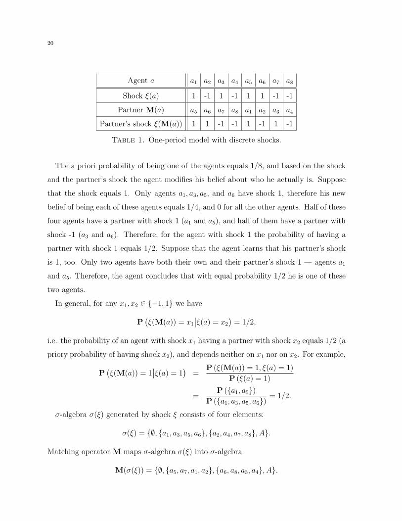
Suppose that the shocks and partners are determined by Table 1.

20

Agent a a1 a2 a3 a4 a5 a6 a7 a8

Shock ξ(a) 1 -1 1 -1 1 1 -1 -1

Partner M(a) a5 a6 a7 a8 a1 a2 a3 a4

Partner’s shock ξ(M(a)) 1 1 -1 -1 1 -1 1 -1

Table 1. One-period model with discrete shocks.

The a priori probability of being one of the agents equals 1/8, and based on the shock

and the partner’s shock the agent modifies his belief about who he actually is. Suppose

that the shock equals 1. Only agents a1, a3, a5, and a6 have shock 1, therefore his new

belief of being each of these agents equals 1/4, and 0 for all the other agents. Half of these

four agents have a partner with shock 1 (a1 and a5), and half of them have a partner with

shock -1 (a3 and a6). Therefore, for the agent with shock 1 the probability of having a

partner with shock 1 equals 1/2. Suppose that the agent learns that his partner’s shock

is 1, too. Only two agents have both their own and their partner’s shock 1 — agents a1

and a5. Therefore, the agent concludes that with equal probability 1/2 he is one of these

two agents.

In general, for any x1, x2 ∈ −1, 1 we have

P(

ξ(M(a)) = x1

∣

∣ξ(a) = x2

)

= 1/2,

i.e. the probability of an agent with shock x1 having a partner with shock x2 equals 1/2 (a

priory probability of having shock x2), and depends neither on x1 nor on x2. For example,

P(

ξ(M(a)) = 1∣

∣ξ(a) = 1)

=P (ξ(M(a)) = 1, ξ(a) = 1)

P (ξ(a) = 1)

=P (a1, a5)

P (a1, a3, a5, a6)= 1/2.

σ-algebra σ(ξ) generated by shock ξ consists of four elements:

σ(ξ) = ∅, a1, a3, a5, a6, a2, a4, a7, a8, A.

Matching operator M maps σ-algebra σ(ξ) into σ-algebra

M(σ(ξ)) = ∅, a5, a7, a1, a2, a6, a8, a3, a4, A.

21

It is easy to show that any two sets from σ(ξ) and M(σ(ξ)) are independent, which means

that the agent’s shock is independent of the partner’s shock, and the value of the agent’s

shock does not change his belief about the shock of his partner.

One-Period Model with Continuous Shocks

For any distribution function F (·) there always exists a probability space A with two

independent random variables ξ1 and ξ2 distributed in accordance with cdf F (·). Take A1

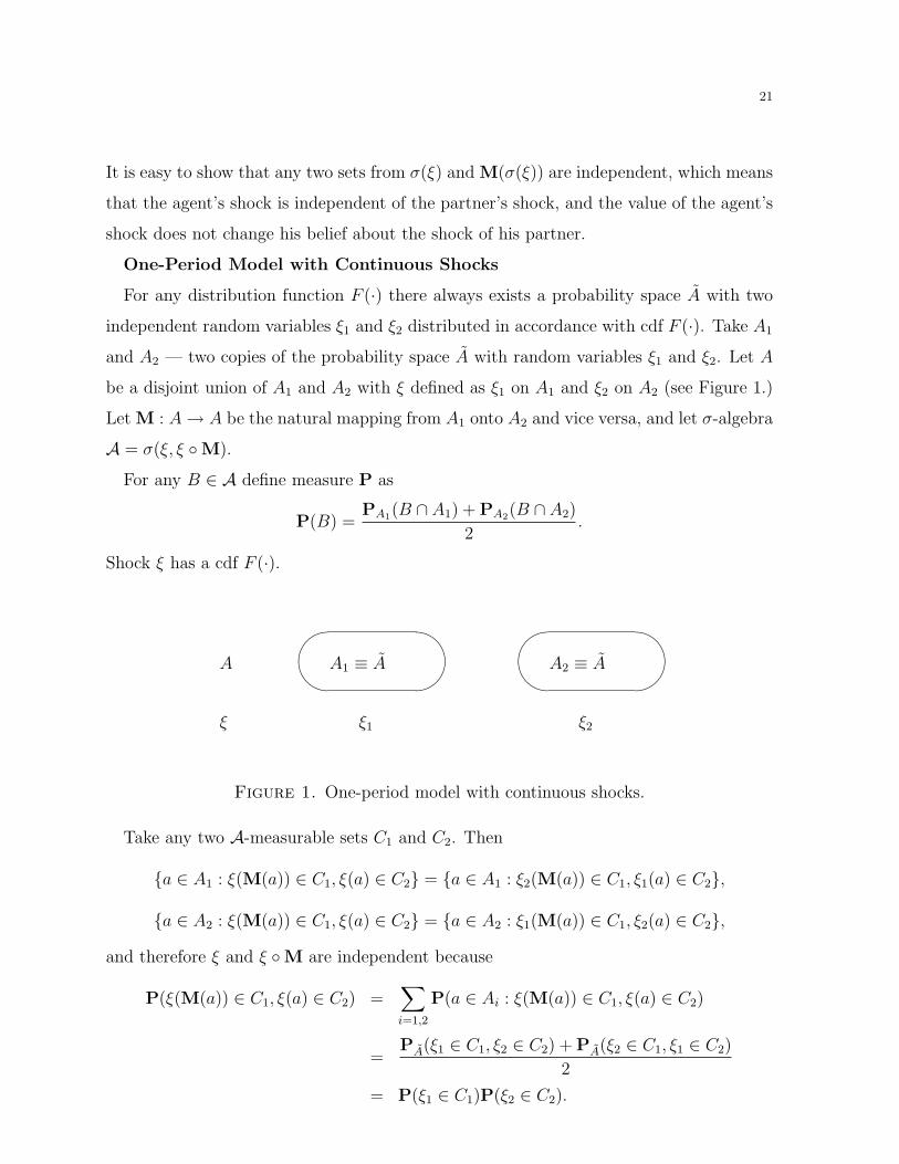
and A2 — two copies of the probability space A with random variables ξ1 and ξ2. Let A

be a disjoint union of A1 and A2 with ξ defined as ξ1 on A1 and ξ2 on A2 (see Figure 1.)

Let M : A → A be the natural mapping from A1 onto A2 and vice versa, and let σ-algebra

A = σ(ξ, ξ M).

For any B ∈ A define measure P as

P(B) =PA1

(B ∩ A1) + PA2(B ∩ A2)

2.

Shock ξ has a cdf F (·).

A1 ≡ A A2 ≡ AA

ξ1 ξ2ξ

Figure 1. One-period model with continuous shocks.

Take any two A-measurable sets C1 and C2. Then

a ∈ A1 : ξ(M(a)) ∈ C1, ξ(a) ∈ C2 = a ∈ A1 : ξ2(M(a)) ∈ C1, ξ1(a) ∈ C2,

a ∈ A2 : ξ(M(a)) ∈ C1, ξ(a) ∈ C2 = a ∈ A2 : ξ1(M(a)) ∈ C1, ξ2(a) ∈ C2,

and therefore ξ and ξ M are independent because

P(ξ(M(a)) ∈ C1, ξ(a) ∈ C2) =∑

i=1,2

P(a ∈ Ai : ξ(M(a)) ∈ C1, ξ(a) ∈ C2)

=PA(ξ1 ∈ C1, ξ2 ∈ C2) + PA(ξ2 ∈ C1, ξ1 ∈ C2)

2

= P(ξ1 ∈ C1)P(ξ2 ∈ C2).

22

The examples considered in this section demonstrate the main idea of the construction

of idiosyncratic shocks and random matchings: the agents do not know who they are,

and based on the previous event (their own shocks) the agents are not able to infer any

additional information about their future (partners’ shocks).

5. Idiosyncratic Shocks and Random Matchings

This section defines idiosyncratic shocks and random matchings using independence of

the history. We prove that there exists a space with a sequence of idiosyncratic shocks

and random matchings (the random matchings are anonymous and commutative). We

show how the old assumptions relate to the new ones.

5.1. Basic Definitions

Consider an agent space (A,A, µ). The same space serves as the probability space:

Ω = A, F = A, and P = µ. The uncertainty an agent faces comes from his unknown

identity a ∈ A.

Definition. A shock is a random variable on (A,A, µ).

The definition of a random matching consists of three parts: matching operator, mea-

sure preservation, and independence.

Definition. A matching operator is an operator M : A → A with the following

properties:

C1. M is a bijection:

∀ a ∈ A ∃! a′ ∈ A : M(a′) = a;

C2. No agent meets himself:

∀ a ∈ A M(a) 6= a;

C3. The partner’s partner is the agent himself:

M−1 = M.

Definition. A matching operator M is measurable if

C4. It maps measurable sets into measurable sets:

∀B ∈ A M−1(B) ∈ A.

23

Definition. A measurable matching operator M is measure-preserving if

C5. It does not change the measure of any measurable subset:

∀B ∈ A µ(M−1(B)) = µ(B).

Before proceeding with defining the concepts of idiosyncratic shocks and random match-

ings, we need the concept of history in order to capture the idea of independence of the

current events from the past.

5.2. History

Time is discrete, t ∈ T ≡ Z. A sequence of shocks ξtt∈T and measure-preserving

matching operators Mtt∈T is given. At the beginning of each period, the agents expe-

rience shocks, and at the end of each period they meet.

Wither the agents can infer any additional information about the future depends on how

much they remember from the past. The information available to an agent at each period

of time is called history. We assume that the agent’s own shocks and the information

sharing during the meetings is the only possible source for the history. We denote the

agent a’s history measured right before the meeting by Ht(a), and right before the shock

by H ′t(a).

Let At be the minimal σ-algebra in which history Ht(a) is a measurable function:

At = σ(Ht(·)), and A′t be the minimal σ-algebra in which history H ′

t(a) is a measurable

function: A′t = σ(H ′

t(·)). We say that sigma-algebras At and A′t are generated by the

history.40 The shocks and matchings are A-measurable, therefore At,A′t ⊂ A.

If the agents remember everything and during the meetings they share their full histo-

ries, then history HMt(a) is called maximal history and includes:

1. Current shock ξt(a);

2. History at the previous period of time HMt−1(a);

3. Previous period partner’s history HMt−1(Mt−1(a)).

40This definition helps us to avoid the problem of dynamic coalition formation mentioned by Alos-

Ferrer [5] “it would be expected that any large coalition of traders could be able to form a risk-pooling

coalition.” The same problem is stated in footnote 4 “it is important to keep track of the sets of agents

that have experienced a specific realization.” The problem is avoided by defining a sequence of σ-algebras.

24

Therefore,

HMt(a) = (ξt(a), HMt−1(a), HMt−1(Mt−1(a)). (3)

The maximal history before the shock equals

H ′Mt(a) = (HMt−1(a), HMt−1(Mt−1(a)). (4)

Since the shocks and meetings is the only source for the history, from equation 3 follows

AMt ≡ σ(HMt(·)) = σ(ξt,AMt−1,Mt−1(AMt−1))

= σ(

ξt, ξt0 Mt1 Mt2 . . . Mtlt0≤t1<t2<...<tl<t

)

.

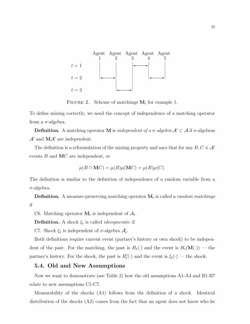
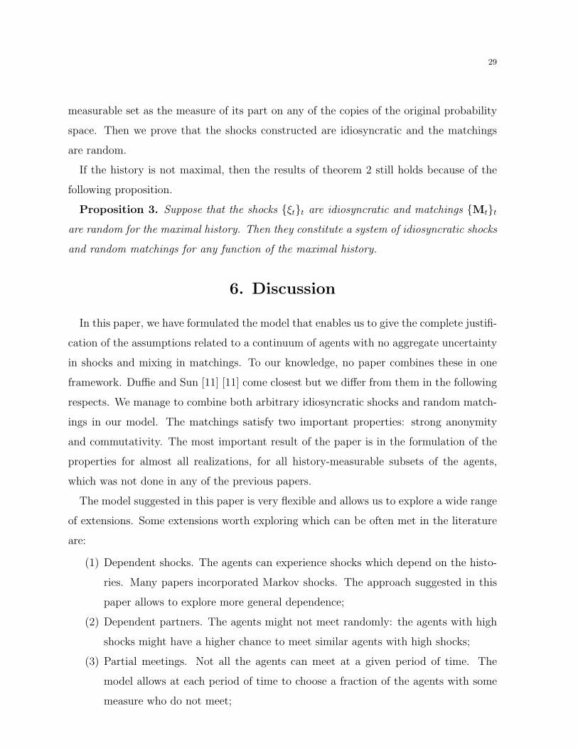
Example 1. Suppose that Agent 3 meets with Agent 4 at period 1 and with Agent

2 at period 3 (see Figure 2.) Suppose also that Agent 2 meets with Agent 1 at Period 2,

and Agent 4 meets with Agent 5 at period 2.

Then for the maximal history at the end of period 3 (after the matching) Agent 3 knows

Agent 4’s history up to period 1 (when they met), Agent 2’s history up to period 3, and

Agent 1’s history up to period 2 (when Agent 2 met Agent 1). At the same time, Agent

3 at the end of period 3 does not know anything about Agent 5 because their common

partner — Agent 4 — met with Agent 3 before he met Agent 5.

Denoting the agents as a1, a2, a3, a4, and a5 correspondingly, we can write:

M1(a3) = a4; M2(a1) = a2; M2(a4) = a5; M3(a2) = a3,

and maximal histories

HM3(a2) = (ξ3(a2), ξ2(a2), ξ1(a2), ξ2(a1), ξ1(a1));

HM3(a3) = (ξ3(a3), ξ2(a3), ξ1(a3), ξ1(a4)).

5.3. Independence

Mixing property B8 was not defined correctly because no measure-preserving matching

operator can be mixing on the whole non-trivial σ-algebra A.41 At the same time, if

we consider a family of σ-algebras At generated by the history, then the sequence of

matching operators Mt can be mixing in the sense of Mt being mixing on At for each t.

41See “A Measure Preserving Matching can not be Mixing” inconsistency, page 16.

25

t = 3

t = 2

t = 1

Agent1

Agent2

Agent3

Agent4

Agent5

Figure 2. Scheme of matchings Mt for example 1.

To define mixing correctly, we need the concept of independence of a matching operator

from a σ-algebra.

Definition. A matching operator M is independent of a σ-algebra A′ ⊂ A if σ-algebras

A′ and MA′ are independent.

The definition is a reformulation of the mixing property and says that for any B, C ∈ A′

events B and MC are independent, or

µ(B ∩ MC) = µ(B)µ(MC) = µ(B)µ(C).

The definition is similar to the definition of independence of a random variable from a

σ-algebra.

Definition. A measure-preserving matching operator Mt is called a random matchings

if

C6. Matching operator Mt is independent of At.

Definition. A shock ξt is called idiosyncratic if

C7. Shock ξt is independent of σ-algebra A′t.

Both definitions require current event (partner’s history or own shock) to be indepen-

dent of the past. For the matching, the past is Ht(·) and the event is Ht(M(·)) — the

partner’s history. For the shock, the past is H ′t(·) and the event is ξt(·) — the shock.

5.4. Old and New Assumptions

Now we want to demonstrate (see Table 2) how the old assumptions A1-A4 and B1-B7

relate to new assumptions C1-C7.

Measurability of the shocks (A1) follows from the definition of a shock. Identical

distribution of the shocks (A2) comes from the fact that an agent does not know who he

26

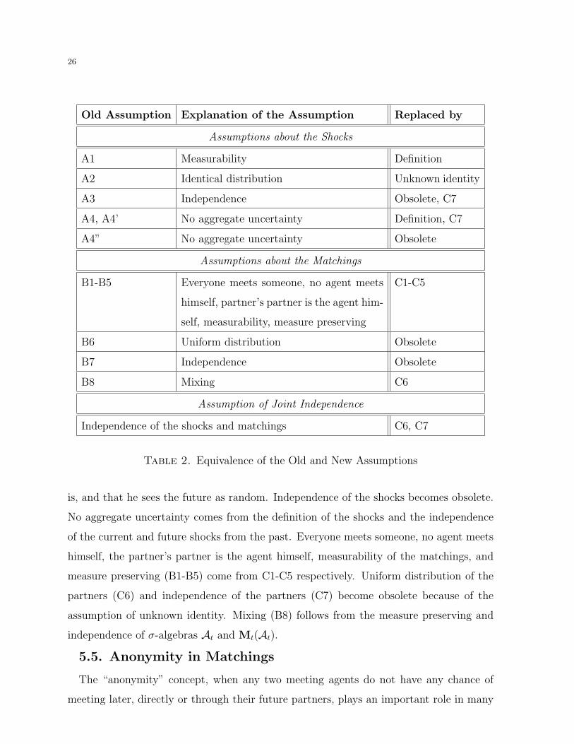
Old Assumption Explanation of the Assumption Replaced by

Assumptions about the Shocks

A1 Measurability Definition

A2 Identical distribution Unknown identity

A3 Independence Obsolete, C7

A4, A4’ No aggregate uncertainty Definition, C7

A4” No aggregate uncertainty Obsolete

Assumptions about the Matchings

B1-B5 Everyone meets someone, no agent meets

himself, partner’s partner is the agent him-

self, measurability, measure preserving

C1-C5

B6 Uniform distribution Obsolete

B7 Independence Obsolete

B8 Mixing C6

Assumption of Joint Independence

Independence of the shocks and matchings C6, C7

Table 2. Equivalence of the Old and New Assumptions

is, and that he sees the future as random. Independence of the shocks becomes obsolete.

No aggregate uncertainty comes from the definition of the shocks and the independence

of the current and future shocks from the past. Everyone meets someone, no agent meets

himself, the partner’s partner is the agent himself, measurability of the matchings, and

measure preserving (B1-B5) come from C1-C5 respectively. Uniform distribution of the

partners (C6) and independence of the partners (C7) become obsolete because of the

assumption of unknown identity. Mixing (B8) follows from the measure preserving and

independence of σ-algebras At and Mt(At).

5.5. Anonymity in Matchings

The “anonymity” concept, when any two meeting agents do not have any chance of

meeting later, directly or through their future partners, plays an important role in many

27

economic models. 42 The anonymity implies that the current action of an agent can not

influence his future. We want to establish how idiosyncratic shocks and random matchings

are related to the concept of anonymity.

Following Aliprantis et al. [2], we define the concepts of indirect partners and strongly

anonymous matchings.43

Definition. We define the set of indirect partners of agent a at time t (before the

matching) as follows:

Ht(a) = a ∪ Mt1 Mt2 . . . Mtl(a)t1<t2<...<tl<t

.

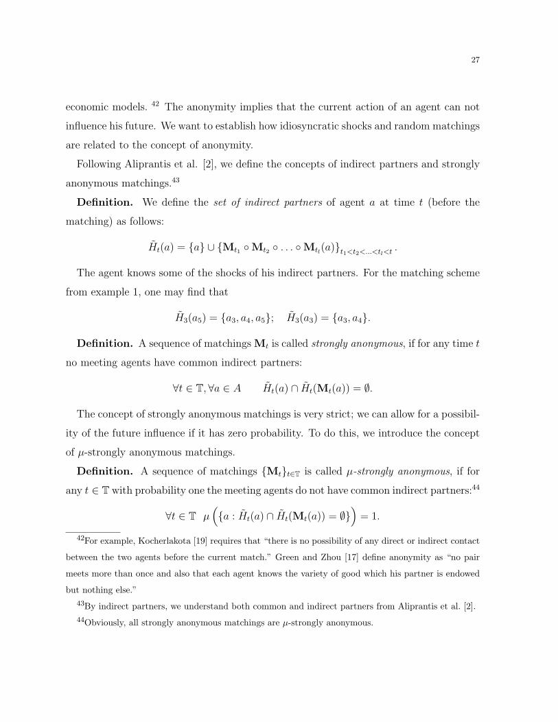
The agent knows some of the shocks of his indirect partners. For the matching scheme

from example 1, one may find that

H3(a5) = a3, a4, a5; H3(a3) = a3, a4.

Definition. A sequence of matchings Mt is called strongly anonymous, if for any time t

no meeting agents have common indirect partners:

∀t ∈ T,∀a ∈ A Ht(a) ∩ Ht(Mt(a)) = ∅.

The concept of strongly anonymous matchings is very strict; we can allow for a possibil-

ity of the future influence if it has zero probability. To do this, we introduce the concept

of µ-strongly anonymous matchings.

Definition. A sequence of matchings Mtt∈T is called µ-strongly anonymous, if for

any t ∈ T with probability one the meeting agents do not have common indirect partners:44

∀t ∈ T µ(

a : Ht(a) ∩ Ht(Mt(a)) = ∅)

= 1.

42For example, Kocherlakota [19] requires that “there is no possibility of any direct or indirect contact

between the two agents before the current match.” Green and Zhou [17] define anonymity as “no pair

meets more than once and also that each agent knows the variety of good which his partner is endowed

but nothing else.”

43By indirect partners, we understand both common and indirect partners from Aliprantis et al. [2].

44Obviously, all strongly anonymous matchings are µ-strongly anonymous.

28

The next theorem demonstrates that the random matchings for the maximal history

should be µ-strongly anonymous.45 If the history differs from the maximal history, the

requirement of µ-strong anonymity can be weakened.

Theorem 1. Let F (·) be a continuous distribution function. Then the matchings are

random for the maximal history only if they are µ-strongly anonymous.

5.6. Existence

The following theorem constitutes the main result of the paper. It establishes the

existence of a sequence of idiosyncratic shocks and random matchings for the maximal

history as we defined them before.

Theorem 2. For any F (·) there exists a probability space (A,A, µ) with a continuum

of elements. On this probability space there exists a sequence of idiosyncratic shocks ξt and

random matchings Mt for the maximal history. The matchings are strongly anonymous

and commutative: for any t1, t2 holds

Mt1 Mt2 = Mt2 Mt1 .

The idea of the proof is the following. We construct a probability space with a sufficient

number of random independent variables. Then, we create countably many copies of this

space and allocate the random variables to these spaces. The agent space is the union of

all the copies, and the shock at each period of time is a particular random variable on the

corresponding copy of the original probability space. At each period of time, the agents

from one copy of the probability space meet with the corresponding agents from some

other copy. The copies whose agents meet are chosen in such a way that the matchings are

strongly anonymous; to achieve this, we use Aliprantis et al. [3] mechanism of recursive

block-partition on the copies of the probability space. The σ-algebra is generated by

the shocks and matchings; the σ-algebras at each period of time are generated by the

histories. It turns out that for any measurable set on the agent space its original measure

on any of the copies does not depend on the copy. Therefore, we define the measure of a

45In Theorem 2 we show that spaces with idiosyncratic shocks and strongly anonymous random match-

ings exist. Hence, we do not need to consider any other types of anonymity because, as was shown in

Aliprantis et al. [3], all of them follow from strong anonymity.

29

measurable set as the measure of its part on any of the copies of the original probability

space. Then we prove that the shocks constructed are idiosyncratic and the matchings

are random.

If the history is not maximal, then the results of theorem 2 still holds because of the

following proposition.

Proposition 3. Suppose that the shocks ξtt are idiosyncratic and matchings Mtt

are random for the maximal history. Then they constitute a system of idiosyncratic shocks

and random matchings for any function of the maximal history.

6. Discussion

In this paper, we have formulated the model that enables us to give the complete justifi-

cation of the assumptions related to a continuum of agents with no aggregate uncertainty

in shocks and mixing in matchings. To our knowledge, no paper combines these in one

framework. Duffie and Sun [11] [11] come closest but we differ from them in the following

respects. We manage to combine both arbitrary idiosyncratic shocks and random match-

ings in our model. The matchings satisfy two important properties: strong anonymity

and commutativity. The most important result of the paper is in the formulation of the

properties for almost all realizations, for all history-measurable subsets of the agents,

which was not done in any of the previous papers.

The model suggested in this paper is very flexible and allows us to explore a wide range

of extensions. Some extensions worth exploring which can be often met in the literature

are:

(1) Dependent shocks. The agents can experience shocks which depend on the histo-

ries. Many papers incorporated Markov shocks. The approach suggested in this

paper allows to explore more general dependence;

(2) Dependent partners. The agents might not meet randomly: the agents with high

shocks might have a higher chance to meet similar agents with high shocks;

(3) Partial meetings. Not all the agents can meet at a given period of time. The

model allows at each period of time to choose a fraction of the agents with some

measure who do not meet;

30

(4) Non-anonymous matchings. The agents might have a non-zero chance of meeting

the current partner in the future.

31

References

1. Al-Najjar, Nabil I. 2004. “Aggregation and the Law of Large Numbers in Large

Economies.” Games and Economic Behavior 47, pp. 1-35.

2. Aliprantis, Charalambos D., G. Camera, and D. Puzzello. 2006. “Matching and Ano-

nymity.” Economic Theory 29, pp. 415-432.

3. Aliprantis, Charalambos D., G. Camera, and D. Puzzello. 2007. “A Random Matching

Theory.” Games and Economic Behavior 59, pp. 116.

4. Alos-Ferrer, Carlos. 1999. “Dynamical Systems with a Continuum of Randomly

Matched Agents.” J. Econ. Theory 86, pp. 245-267.

5. Alos-Ferrer, Carlos. 2002. “Individual Randomness in Economic Models with a Con-

tinuum of Agents.” Working paper.

6. Alos-Ferrer, Carlos. 2002. “Random Matching of Several Infinite Populations.” An-

nals of Operations Research 114, pp. 33-38.

7. Boylan, Richard T. 1992. “Laws of Large Numbers for Dynamical Systems with

Randomly Matched Individuals.” J. Econ. Theory 57, pp. 473-504.

8. Boylan, Richard T. 1995. “Continuous Approximations of Dynamical Systems with

Randomly Matched Individuals.” J. Econ. Theory 66, pp. 615-625.

9. Doob, J.L.. 1937. “Stochastic processes depending on a continuous parameter.” Trans.

Am. Math. Soc. 42, 107140.

10. Duffie, Darrell, and Yeneng Sun. 2004. “The Exact Law of Large Numbers for Inde-

pendent Random Matching.” Working paper, Graduate School of Business, Stanford

University.

11. Duffie, Darrell, and Yeneng Sun. 2007. “Existence of Independent Random Match-

ing.” Annals of Applied Probability 17, pp. 386-419.

12. Feldman, Mark, and Christian Gilles. 1985. “An Expository Note on Individual Risk

without Aggregate Uncertainty.” J. Econ. Theory 35, pp. 26-32.

13. Feller, William. 1968. “An Introduction to Probability Theory and Its Applications.”

Volume I, Wiley International Edition, New York, 3rd Edition, 510 pp.

14. Gale, Douglas. 1986. “Bargaining and Competition Part I: Characterization.” Econo-

metrica 54(4), pp. 785-806.

32

15. Gilboa, Itzhak, and Akihiko Matsui. 1992. “A Model of Random Matching.” Journal

of Mathematical Economics 21, pp. 185-197.

16. Green, Edward J. 1994. “Individual-Level Randomness in a Nonatomic Population.”

Working paper, University of Minnesota.

17. Green, Edward J., and Ruilin Zhou. 2002. “Dynamic Monetary Equilibrium in a

Random Matching Economy.” Econometrica 70, pp. 929-969.

18. Halmos, Paul. 1974. “Naive set theory.” Springer-Verlag, New York.

19. Judd, Kenneth L. 1985. “The Law of Large Numbers with a Continuum of IID Ran-

dom Variables.” J. Econ. Theory 35, pp. 19-25.

19. Kandori, Michihiro. 1992. “Social Norms and Community Enforcement.” The Review

of Economic Studies 59(1), pp. 63-80.

19. Kocherlakota, Narayana R. 1998. “Money Is Memory.” Journal of Economic Theory

81, pp. 232-251.

20. McLennan, Andrew, and Hugo Sonnenschein. 1991. “Sequential Bargaining as a Non-

cooperative Foundation for Walrasian Equilibrium.” Econometrica 59, pp. 1395-1424.

21. Shi, Shouyong. 1997. “A Divisible Search Model of Fiat Money.” Econometrica 65(1),

pp. 75-102.

22. Sun, Yeneng. 1998. “A Theory of Hyperfinite Processes: the Complete Removal of

Individual Uncertainty via Exact LLN.” Journal of Mathematical Economics 29, pp.

419-503.

23. Uhlig, Harald. 1996. “A Law of Large Numbers for Large Economies.” Economic

Theory 8, pp. 41-50.

24. Wentzell, Alexander D. 1981. “A Course in the Theory of Stochastic Processes.” New

York: McGraw-Hill.

33

Appendix

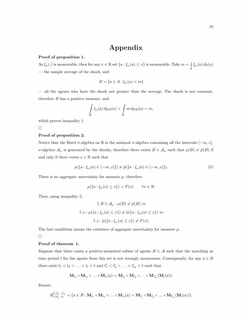
Proof of proposition 1.

As ξω(·) is measurable, then for any x ∈ R set a : ξω(a) ≤ x is measurable. Take m =∫

A

ξω(a) dµ(a)

— the sample average of the shock, and

B = a ∈ A : ξω(a) < m

— all the agents who have the shock not greater than the average. The shock is not constant,

therefore B has a positive measure, and∫

B

ξω(a) dµB(a) <

∫

B

m dµB(a) = m,

which proves inequality 1.

Proof of proposition 2.

Notice that the Borel σ-algebra on R is the minimal σ-algebra containing all the intervals (−∞, x].

σ-algebra Aω is generated by the shocks, therefore there exists B ∈ Aω such that µ(B) 6= µ(B) if

and only if there exists x ∈ R such that

µ(a : ξω(a) ∈ (−∞, x]) 6= µ(a : ξω(a) ∈ (−∞, x]). (5)

There is no aggregate uncertainty for measure µ, therefore

µ(a : ξω(a) ≤ x) = F (x) ∀x ∈ R.

Then, using inequality 5,

∃ B ∈ Aω : µ(B) 6= µ(B) ⇔

∃ x : µ(a : ξω(a) ≤ x) 6= µ(a : ξω(a) ≤ x) ⇔

∃ x : µ(a : ξω(a) ≤ x) 6= F (x).

The last conditions means the existence of aggregate uncertainty for measure µ.

Proof of theorem 1.

Suppose that there exists a positive-measured subset of agents B ∈ A such that the matching at

time period t for the agents from this set is not strongly anonymous. Consequently, for any a ∈ B

there exist t1 < t2 < . . . < tl < t and t′1 < t′2 < . . . < t′m < t such that

Mt1 Mt2 . . . Mtl(a) = Mt′1

Mt′2 . . . Mt′m

(Mt(a)).

Denote

Bt′1t′2...t′mt1t2...tl

= a ∈ B : Mt1 Mt2 . . . Mtl(a) = Mt′1

Mt′2 . . . Mt′m

(Mt(a)).

34

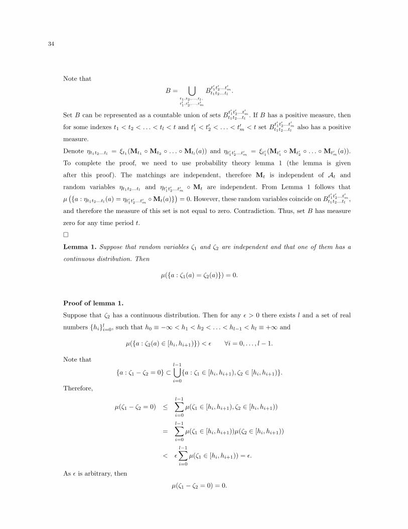
Note that

B =⋃

t1,t2,...,tl,

t′1,t′2,...,t′m

Bt′1t′2...t′mt1t2...tl

.

Set B can be represented as a countable union of sets Bt′1t′2...t′mt1t2...tl

. If B has a positive measure, then

for some indexes t1 < t2 < . . . < tl < t and t′1 < t′2 < . . . < t′m < t set Bt′1t′2...t′mt1t2...tl

also has a positive

measure.

Denote ηt1t2...tl= ξt1(Mt1 Mt2 . . . Mtl

(a)) and ηt′1t′2...t′m= ξt′1

(Mt′1 Mt′2

. . . Mt′m(a)).

To complete the proof, we need to use probability theory lemma 1 (the lemma is given

after this proof). The matchings are independent, therefore Mt is independent of At and

random variables ηt1t2...tland ηt′1t′2...t′m

Mt are independent. From Lemma 1 follows that

µ(

a : ηt1t2...tl(a) = ηt′1t′2...t′m

Mt(a))

= 0. However, these random variables coincide on Bt′1t′2...t′mt1t2...tl

,

and therefore the measure of this set is not equal to zero. Contradiction. Thus, set B has measure

zero for any time period t.

Lemma 1. Suppose that random variables ζ1 and ζ2 are independent and that one of them has a

continuous distribution. Then

µ(a : ζ1(a) = ζ2(a)) = 0.

Proof of lemma 1.

Suppose that ζ2 has a continuous distribution. Then for any ǫ > 0 there exists l and a set of real

numbers hili=0, such that h0 ≡ −∞ < h1 < h2 < . . . < hl−1 < hl ≡ +∞ and

µ(a : ζ2(a) ∈ [hi, hi+1)) < ǫ ∀i = 0, . . . , l − 1.

Note that

a : ζ1 − ζ2 = 0 ⊂l−1⋃

i=0

a : ζ1 ∈ [hi, hi+1), ζ2 ∈ [hi, hi+1).

Therefore,

µ(ζ1 − ζ2 = 0) ≤l−1∑

i=0

µ(ζ1 ∈ [hi, hi+1), ζ2 ∈ [hi, hi+1))

=

l−1∑

i=0

µ(ζ1 ∈ [hi, hi+1))µ(ζ2 ∈ [hi, hi+1))

< ǫ

l−1∑

i=0

µ(ζ1 ∈ [hi, hi+1)) = ǫ.

As ǫ is arbitrary, then

µ(ζ1 − ζ2 = 0) = 0.

35

Proof of theorem 2.

Agent Space

By Kolmogorov theorem, for any distribution function F (·) there exists a probability space (Θ,Q, ν)

with a countable number of independent random variables ξiti∈N,t∈T, each distributed in accor-

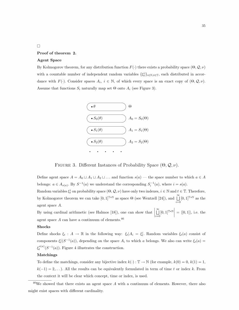
dance with F (·). Consider spaces Ai, i ∈ N, of which every space is an exact copy of (Θ,Q, ν).

Assume that functions Si naturally map set Θ onto Ai (see Figure 3).

r r r rθ Θ

S0(θ) A0 = S0(Θ)

S1(θ) A1 = S1(Θ)

S2(θ) A2 = S2(Θ)

q q q q qFigure 3. Different Instances of Probability Space (Θ,Q, ν).

Define agent space A = A0 ⊔ A1 ⊔ A2 ⊔ . . . and function s(a) — the space number to which a ∈ A

belongs: a ∈ As(a). By S−1(a) we understand the corresponding S−1i (a), where i = s(a).

Random variables ξit on probability space (Θ,Q, ν) have only two indexes, i ∈ N and t ∈ T. Therefore,

by Kolmogorov theorem we can take [0, 1]T∗N as space Θ (see Wentzell [24]), and∞⊔

i=0

[0, 1]T∗N as the

agent space A.

By using cardinal arithmetic (see Halmos [18]), one can show that

∣

∣

∣

∣

∞⊔

i=0

[0, 1]T∗N

∣

∣

∣

∣

= |[0, 1]|, i.e. the

agent space A can have a continuum of elements.46

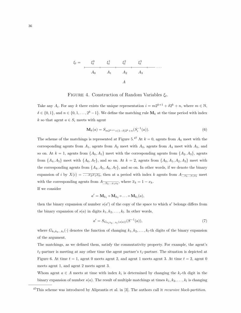
Shocks

Define shocks ξt : A → R in the following way: ξt|Ai = ξit. Random variables ξt(a) consist of

components ξit(S

−1(a)), depending on the space Ai to which a belongs. We also can write ξt(a) =

ξs(a)t (S−1(a)). Figure 4 illustrates the construction.

Matchings

To define the matchings, consider any bijective index k(·) : T → N (for example, k(0) = 0, k(1) = 1,

k(−1) = 2,. . . ). All the results can be equivalently formulated in term of time t or index k. From

the context it will be clear which concept, time or index, is used.

46We showed that there exists an agent space A with a continuum of elements. However, there also

might exist spaces with different cardinality.

36

A

A0 A1 A2 A3

ξt = ξ0t ξ1

t ξ2t ξ3

t ♣ ♣ ♣

Figure 4. Construction of Random Variables ξt.

Take any Ai. For any k there exists the unique representation i = m2k+1 + δ2k + n, where m ∈ N,

δ ∈ 0, 1, and n ∈ 0, 1, . . . , 2k −1. We define the matching rule Mk at the time period with index

k so that agent a ∈ Si meets with agent

Mk(a) = Sm2k+1+(1−δ)2k+n(S−1i (a)). (6)

The scheme of the matchings is represented at Figure 5.47 At k = 0, agents from A0 meet with the

corresponding agents from A1, agents from A2 meet with A3, agents from A4 meet with A5, and

so on. At k = 1, agents from A0, A1 meet with the corresponding agents from A2, A3, agents

from A4, A5 meet with A6, A7, and so on. At k = 2, agents from A0, A1, A2, A3 meet with

the corresponding agents from A4, A5, A6, A7, and so on. In other words, if we denote the binary

expansion of i by X(i) = . . . x2x1x0, then at a period with index k agents from A...xk...x1x0meet

with the corresponding agents from A...xk...x1x0, where xk = 1 − xk.

If we consider

a′ = Mk1 Mk2 . . . Mkl(a),

then the binary expansion of number s(a′) of the copy of the space to which a′ belongs differs from

the binary expansion of s(a) in digits k1, k2, . . . , kl. In other words,

a′ = SGk1k2...kl(s(a))(S

−1(a)), (7)

where Gk1k2...kl(·) denotes the function of changing k1, k2, . . . , kl-th digits of the binary expansion

of the argument.

The matchings, as we defined them, satisfy the commutativity property. For example, the agent’s

t1-partner is meeting at any other time the agent partner’s t1-partner. The situation is depicted at

Figure 6. At time t = 1, agent 0 meets agent 2, and agent 1 meets agent 3. At time t = 2, agent 0

meets agent 1, and agent 2 meets agent 3.

Whom agent a ∈ A meets at time with index ki is determined by changing the ki-th digit in the

binary expansion of number s(a). The result of multiple matchings at times k1, k2, . . . , kl is changing

47This scheme was introduced by Aliprantis et al. in [3]. The authors call it recursive block-partition.

37

k = 0

k = 1

k = 2

A0 A1 A2 A3 A4 A5 A6 A7

A0 A1 A2 A3 A4 A5 A6 A7

A0 A1 A2 A3 A4 A5 A6 A7

Figure 5. The Structure of the Matchings.

t = 2

t = 1

Agent0

Agent1

Agent2

Agent3

Figure 6. Commutativity of matchings.

digits k1, k2, . . . , kl in the binary expansion of s(a). For any permutation of the times the result is

the same because it does not matter in which order to change the digits. Therefore, for any set of

time indexes k1, k2, . . . , kl and for any permutation τ of numbers 1, 2, . . . , l, the following equation

(commutativity of matchings) holds:

Mk1 Mk2

. . . Mkl≡ Mkτ(1)

Mkτ(2) . . . Mkτ(l)

.

The matchings are strongly anonymous because of the commutativity: if agent a meets agent

a′ = Mk0(a) at time with index k0 and they have a common previous indirect partner, then

Mk1 Mk2

. . . Mkl(a) = Mk′

1 Mk′

2 . . . Mk′

m(a′);

38

Mk′

1 Mk′

2 . . . Mk′

m Mk1

Mk2 . . . Mkl

(a) = a′ ≡ Mk0(a) (8)

for some sets k1, k2, . . . , kl and k′1, k

′2, . . . , k

′m. Matching at time ki corresponds to changing

ki-digit in the binary expansion of the space number to which a belongs. Therefore equation 8

holds only on such sets k1, k2, . . . , kl and k′1, k

′2, . . . , k

′m that differ in one element k0, which is

impossible because the previous partners could not meet at time k0.

σ-Algebra

Following the definition, σ-algebras At and A′t are generated by the maximal history:

At = σ(

ξt, ξt0 Mt1 Mt2 . . . Mtlt0≤t1<t2<...<tl<t

)

;

A′t = σ

(

At−1,Mt−a(A′t−1)

)

.

Note that At ⊆ A′t+1 ⊆ At+1. Define σ-algebra A as the minimal σ-algebras in which all the shocks

and matchings are measurable:

A = σ(

ξt0 Mt1 . . . Mtlt0,t1,...,tl

)

.

Obviously,

At,A′t ⊆ A.

Probability

In order to define probability measure on (A,A), we will use the probability measure ν on (Θ,Q).

Namely, for any B ∈ A define

µ(B) = limj→∞

1

j + 1

j∑

i=0

ν(S−1(B ∩ Ai)). (9)

Measure µ(B) is defined correctly. Indeed, consider any finite set of indexes W = k0, k1, . . . , kl

and any measurable sets Bk0,k1,...,kl. From equation 7, for any a ∈ Ai

ξt0 Mt1 . . . Mtl(a) = ξ

Gk1k2...kl(i)

t0(S−1(a)).

Hence, values

νi = ν

⋂

(k0,k1,...,kl)∈W

θ ∈ Θ : ξk0 Mk1 . . . Mkl(Si(θ)) ∈ Bk0,k1,...,kl

= ν

⋂

(k0,k1,...,kl)∈W

θ ∈ Θ : ξGk1k2...kl

(i)t0

(θ) ∈ Bk0,k1,...,kl

do not depend on i because of the independence of the random variables

ξGk1k2...kl

(i)t0

(·)

. Therefore,

for any i and j and for any B ∈ A holds

ν(S−1(B ∩ Aj)) = ν(S−1(B ∩ Ai)), (10)

39

which means that measure µ(·) was defined correctly, and for any i

µ(B) = ν(S−1(B ∩ Ai)).

A

⑦ ⑦ ⑦ ⑦A0 A1 A2 A3

s s s s

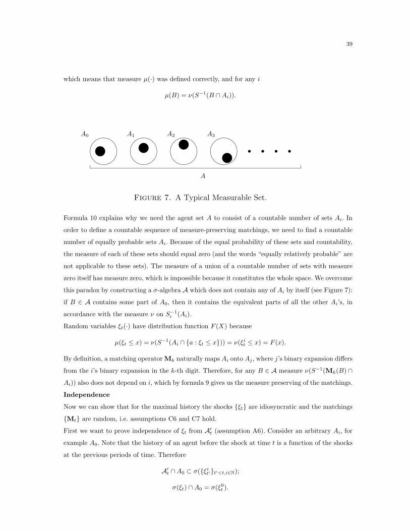
Figure 7. A Typical Measurable Set.

Formula 10 explains why we need the agent set A to consist of a countable number of sets Ai. In

order to define a countable sequence of measure-preserving matchings, we need to find a countable

number of equally probable sets Ai. Because of the equal probability of these sets and countability,

the measure of each of these sets should equal zero (and the words “equally relatively probable” are

not applicable to these sets). The measure of a union of a countable number of sets with measure

zero itself has measure zero, which is impossible because it constitutes the whole space. We overcome

this paradox by constructing a σ-algebra A which does not contain any of Ai by itself (see Figure 7):

if B ∈ A contains some part of A0, then it contains the equivalent parts of all the other Ai’s, in

accordance with the measure ν on S−1i (Ai).

Random variables ξt(·) have distribution function F (X) because

µ(ξt ≤ x) = ν(S−1(Ai ∩ a : ξt ≤ x)) = ν(ξit ≤ x) = F (x).

By definition, a matching operator Mk naturally maps Ai onto Aj , where j’s binary expansion differs

from the i’s binary expansion in the k-th digit. Therefore, for any B ∈ A measure ν(S−1(Mk(B) ∩

Ai)) also does not depend on i, which by formula 9 gives us the measure preserving of the matchings.

Independence

Now we can show that for the maximal history the shocks ξt are idiosyncratic and the matchings

Mt are random, i.e. assumptions C6 and C7 hold.

First we want to prove independence of ξt from A′t (assumption A6). Consider an arbitrary Ai, for

example A0. Note that the history of an agent before the shock at time t is a function of the shocks

at the previous periods of time. Therefore

A′t ∩ A0 ⊂ σ(ξi

t′t′<t,i∈N);

σ(ξt) ∩ A0 = σ(ξ0t ).

40

Since random variables ξit are independent, we have

σ(ξitt<t,i∈N)⊥σ(ξ0

t );

A′t ∩ A0⊥σ(ξt) ∩ A0,

and therefore ξt is independent of A′t on A0, which in accordance with formula 9 means that ξt is

independent of A′t, and therefore shocks ξt are idiosyncratic.

To prove independence of Mt from At (assumption A7), note that the history of an agent from A0

includes his current shock and the shocks of his previous direct or indirect partners. These previous

direct or indirect partners belong to such Ai that xk(t)(i) = 0. The history of an A0 agent’s partner

at time t includes this partner’s current shock and the shocks of this partner’s indirect partners.

These previous indirect partners belong to such Ai that xk(t)(i) = 1. Therefore

At ∩ A0 ⊂ σ(ξit′t′≤t,xk(t)(i)=0);

(At Mt) ∩ A0 ⊂ σ(ξit′t′≤t,xk(t)(i)=1).

Since random variables ξit are independent, we have

(At ∩ A0)⊥(At Mt ∩ A0);

At⊥(At Mt);

Mt⊥At,

i.e. the matching operators are random.

Proof of proposition 3.

Any functions of two independent variables are independent, too. Therefore, the shocks are id-

iosyncratic and the matchings are random under any history which is a function of the maximal

history.