Embed Size (px)
Citation preview

Munich Personal RePEc Archive
Stock Returns Predictability and the
Adaptive Market Hypothesis: Evidence
from India
Hiremath, Gourishankar S and Kumari, Jyoti
Indian Institute of Technology Kharagpur
19 November 2013
Online at https://mpra.ub.uni-muenchen.de/52581/
MPRA Paper No. 52581, posted 09 Feb 2014 05:52 UTC

2
Stock Returns Predictability and the Adaptive Market Hypothesis: Evidence from India
Gourishankar S. Hiremath and Jyoti Kumari
Department of Humanities and Social Sciences
Indian Institute of Technology Kharagpur
Kharagpur – 721302. India
Email ID: [email protected]
Abstract The present paper evaluates whether the adaptive market hypothesis provides a better
description of the behavior of Indian stock market using daily values of Sensex and Nifty, the
two major indices of India from January 1991 to April 2013. We employed linear and nonlinear
methods to evaluate the hypothesis empirically. The linear tests show a cyclical pattern in linear
dependence suggesting that the Indian stock market switched between periods of efficiency and
inefficiency. However, the results from nonlinear tests reveal a strong evidence of nonlinearity in
returns throughout the sample period with a sign of the taping magnitude of nonlinear
dependence in the recent period. The findings suggest that Indian stock market is still in the first
stage of AMH and hence calls for an active portfolio management for excess returns.
Keywords: Adaptive market hypothesis, Market efficiency, Random walk, Autocorrelation,
Nonlinearity, Predictability, behavioral finance.

3
Stock Returns Predictability and the Adaptive Market Hypothesis: Evidence from India
There is no theory, which has attracted volumes of research like efficient market
hypothesis (EMH) over four decades. It is the well-known, yet highly controversial theory of
Neoclassical School of Finance which has influenced modern finance in both theory and
practice. Fama (1970), who explicitly formalized EMH states, “A market in which, prices always
‘fully reflect’, available information is called ‘efficient’1. In such a market, when new
information (news) arrives, security prices quickly respond and incorporate all information at
any point of time, and reach a new equilibrium. Moreover, in such efficient markets, collection
of information is costly and there will be no returns on such actions. Hence, it would not be
possible to earn excess returns in an informationally efficient market. Under such conditions,
fundamental or technical analysis cannot outperform a simple strategy of buying and holding
diversified securities. In other words, the EMH rules out any active portfolio management2.
Despite a large body of research on EMH both from developed and developing markets,
the consensus on this issue that whether markets are efficient or not, thus continues to be elusive.
In recent years, although there is striking evidence that stock returns do not follow random walk
and possess some component of predictability, there is a lack of strong alternative theoretical
explanations to EMH. Nevertheless, recently Lo (2004) has proposed an adaptive market
hypothesis (AMH) based on an evolutionary approach to economic interaction, which can
coexist with EMH in an intellectually consistent manner. It is stated that the emerging and
developing markets have more tendency to reject EMH because of several market frictions.
Unlike EMH which assumes a frictionless market, AMH accommodates market frictions and
1 The seminal work of Bachelier (1900) laid theoretical foundation for the theory of efficient market. The pioneering
work of Samuelson (1965) added rigour to the theory of stock market efficiency. 2 Malkiel (1973) writes to the extent that ‘a blindfolded chimpanzee throwing darts at the Wall Street could select a
portfolio that would do as well as the experts’.

4
asserts that market evolve over a period of time. In light of this, the present article aims to
determine whether AMH provides a better description of the Indian stock market, one of the
emerging markets. To the best of our knowledge, there are no studies of this kind in India.
The remainder of the article is structured as follows. Section 2 provides a brief overview
of adaptive market hypothesis and previous work. Section 3 describes data and econometric
methods implemented for estimations. Section 4 discusses the main results and evaluates the
relevance of adaptive market hypothesis for India. Section 5 concludes.
2. Adaptive Market Hypothesis
Lo (2004) offers an alternative market theory to EMH from a behavioral perspective,
according to which, markets are adaptable and the markets switch between efficiency and
inefficiency at different points of time. Lo (2004) applies the evolutionary approach of biology to
economic interaction and explains the adaptive nature of the agents and consequently how
market becomes adaptive. According to Lo (2005), “degree of market efficiency is related to
environmental factors characterizing market ecology such as the number of competitors, the
magnitude of profit opportunities available, and the adaptability of the market participants. In
contrast to EMH, which assumes a frictionless market, AMH asserts that the laws of natural
selection or “survival of the richest” determines the evolution of markets and institutions in real
world markets which have frictions.
Unlike investors in efficient markets, investors do make mistakes and then they learn and
adapt their behavior accordingly in the framework of AMH. The AMH has a number of practical
implications. First, the risk-reward relationship changes over time because of the preferences of
the populations in the market. Second, the movement of past prices influences the current
preferences because of the forces of natural selection. This contrasts the weak form of efficiency

5
where history of prices are of no use. Third, in adaptive market, arbitrage opportunities do exist
from time to time. From an evolutionary perspective, the profit opportunities are being
constantly created and disappear. This calls for investment strategies according to the market
environment. In other words, AMH implies “complex market dynamics” which necessitates the
active portfolio management. Fourth, innovation is a key to survival and AMH suggest that
adapting to changing market conditions ensures a consistent level of expected returns. Finally,
market efficiency is not an all or none condition but a characteristic that varies continuously over
time and across markets3. Hence, a financial market may witness the periods of efficiency and
inefficiency.
The AMH though still in its infancy, is attracting attention from researchers. Ito and
Sugiyama (2009) find time varying market inefficiency in the US. Charles et al. (2010) holds
AMH true in case foreign exchange rates of developing countries where they find episodes of
return predictability depending on market conditions. Kim et al. (2011) tests whether the US
stock market evolves over time in the US. They find market conditions as the driving factors of
predictability and market is more efficient after 1980s than the previous periods. Exploring the
relative efficiency, Noda (2012) concludes that TOPIX support AMH while TSE2 does not in
Japan. Alvarez-Ramirez et al (2012) provides evidence in favor of AMH and note that the US
market was more efficient during 1973 to 2003. Urquhart and Hudson (2013) document mixed
results for the US, the UK and Japan markets and conclude that the AMH provides a convincing
description of these markets.
3 Campbell et al (1997) note that testing of market efficiency as a condition of all or nothing is not useful and such
an efficient market is the economically unrealizable ideal market. They suggest relative efficiency because
measuring efficiency provides more insights than testing it

6
Given the importance of AMH, the objective of this paper is to examine whether the
Indian stock market evolved over a period of time and does AMH provides convincing
explanations for such an evolution. This assumes importance in the backdrop of the financial
sector reforms in India which were introduced in early 1990s to infuse energy and vibrancy to
the process of economic growth. In addition, the drastic changes in the market microstructure
and trading practices from 1994 onwards sought a transparent, fair and efficient market. As a
result, India’s financial system grew by leaps and bounds. As per the S & P Fact book (2012),
Indian stock market now has the largest number of listed companies on its exchanges. The
growing percentage of market capitalization to the GDP and the increasing integration of the
Indian market with the global economy indicate the phenomenal growth of the Indian equity
market and its growing importance in the economy. The capital market of India emerged as one
of the important destinations for investment. The foreign institutional investors (FIIs) in
particular are highly interested in Indian stock market for portfolio diversification and higher
expected returns. Hence, the Indian stock market has received ample attention from the
international media and academia. Notwithstanding the recent notable growth, investors, traders
and policy-makers have their own misgivings regarding the efficiency of the Indian stock
market.
There are studies which have empirically tested EMH in context of India but the findings
are mixed (E.g. Rao and Mukherjee 1971; Sharma and Kennedy 1977; Barua 1981; Amanulla
and Kamaiah 1998; Poshakwale 2002 among others). Departing from the previous studies on
efficiency of Indian stock market, the present study has made the following improvements. To
the best of our knowledge, this is the first comprehensive work on Indian stock market, which
examines the AMH. Thus, the present article complements literature on AMH and extends

7
existing work that that has examined efficiency of Indian stock market. Besides, the available
studies refer to the 1980s and early 1990s and hence could not capture the changes in the nature
of stock market efficiency in the post-financial sector reform and drastic transformation in
market microstructure of the Indian stock market. The present study covers the period (1991 to
2013) of such changes is in order. Further, the majority of the studies in India used conventional
tests to examine the issue of market efficiency. The present study has employed certain state-of-
the-art methods and techniques, which are first of their kind in the Indian context. Finally, the
issue of nonlinearity in stock returns is addressed in this paper has not received due attention in
India.
2. Methodology
For empirical testing, this study uses daily values of Sensex and Nifty, the major indices
traded in India and together constitute 99 percent of total market capitalization. The Sensex data
is from January 1991 to March 2013 while Nifty data spans from January 1994 and March 2013.
To capture changing efficiency or evolving nature of the market, the whole sample is divided
into two yearly subsamples. Urquhart and Hudson (2013) has proposed a five-type classification
of behavior of stock market returns over time depending on dependence and independence of
returns: efficient, moving towards efficiency, switching to efficiency / inefficiency, adaptive or
inefficient. We use this classification to evaluate the relevance of AMH in explaining stock
returns in India. The present study implements both linear and nonlinear tests for empirical
testing of AMH. The following subsections offers a brief description of these tests.

8
2.1 Linear Tests
2.1.1 Autocorrelation Test
Autocorrelation estimates may be used to test the hypothesis that the process generating
the observed return is a series of independent and identical distribution (iid) of random variables.
It helps to evaluate whether successive values of serial correlation are significantly different
from zero. To test the joint hypothesis that all autocorrelation coefficients are simultaneously
equal to zero, Ljung and Box’s (1978) portmanteau Q-statistic is used in the study. The test
statistic is defined as
2 ∑ ρ . . . (1)
where n is the number of observations, m lag length.The test follows a chi-square ( )
distribution.
2.1.2 Runs Test
Runs test is one of the prominent non-parametric tests of the random walk hypothesis
(RWH). A run is defined as the sequence of consecutive changes in the return series. If the
sequence is positive (negative), it is called positive (negative) run and if there are no changes in
the series, a run is zero. The expected runs are the change in returns required, if a random
process generates the data. If the actual runs are close to the expected number of runs, it indicates
that the returns are generated by a random process. The expected number of runs (ER) is
computed as
ER X X ∑ X . . . (2)
where X is the total number of runs, c is the number of returns changes of each category of sign
(i = 1, 2, 3). The ER in equation (2) has an approximate normal distribution for large X. Hence,
to test the null hypothesis, standard Z statistic can be used4.
4 For further discussion on runs test, see Siegel (1956).

9
2.1.3 Lo and MacKinlay (1988) Variance Ratio Test5
Lo and MacKinaly (1988) proposed the variance ratio test, which is capable of
distinguishing between several interesting alternative stochastic processes. Under RWH for stock
returns r , the variance of r +r are required to be twice the variance of r . Following
Campbell et al (1997), let the ratio of the variance of two period returns, r 2 r r , to
twice the variance of a one-period return r . Then variance ratio VR (2) is
VR 2 V V V V
V C , V
VR 2 1 1 . . . (3)
where ρ (1) is the first order autocorrelation coefficient of returns r . RWH which requires zero
autocorrelations holds true when VR (2) =1. The VR (2) can be extended to any number of
period returns, q. Lo and MackKinaly (1988) showed that the q period variance ratio satisfies the
following relation:
VR V .V 1 2 ∑ 1 . . . (4)
where r r r r and ρ (k) is the kth
order autocorrelation coefficient of
{r . Equation (4) shows that at all q, VR (q) = 1. For random walk to hold, variance ratio is
expected to be equal to unity. The test is based on standard asymptotic approximations. Lo-
MacKinlay proposed Z (q) standard normal test statistic6 under the null hypothesis of
homoscedastic increments and VR (q) =1. However, the rejection of RWH because of
heterscedasticity, which is a common feature of financial returns, is not useful for any practical
5 A detailed discussion on the test and its empirical application can be seen in Campbell et al (1997). 6 A detailed discussion on sampling distribution, size and power of the test can also be found in Lo and MacKinlay
(1999)

10
purpose. Hence, Lo-MacKinlay constructed a heterscedastic robust test statistic Z* (q) which can
be defined as
Z VR ф \ . . . (5)
which follows a standard normal distribution asymptotically. Thus, according to variance ratio
test, the returns process is a random walk when the variance ratio at a holding period q is
expected to be unity. If it is less than unity, it implies negative autocorrelation and if it is greater
than one, indicates positive autocorrelation.
2.1.4 Chow and Denning (1993) Multiple Variance Ratio Test
The variance ratio test of Lo and MacKinlay (1988) estimates individual variance ratios
where one variance ratio is considered at a time, for a particular holding period (q). Empirical
works examine the variance ratio statistics for several q values. The null of the random walk is
rejected if test statistics are significant for some q value. Therefore, it is essentially an individual
hypothesis test. The variance ratio of Lo and MacKinlay (1988) tests whether the variance ratio
is equal to one for a particular holding period, whereas the RWH requires that variance ratios for
all holding periods should be equal to one and the test should be conducted jointly over a number
of holding periods. The sequential procedure of this test leads to size distortions and the test
ignores the joint nature of random walk. To overcome this problem, Chow and Denning (1993)
proposed multiple variance ratio test wherein a set of multiple variance ratios over a number of
holding periods can be tested to determine whether the multiple variance ratios (over a number
of holing periods ) are jointly equal to one. In Lo-MacKinlay test, under the null, VR 1,
but in multiple variance ratio test, – 1 0 . This can be generalized to a
set of m variance ratio tests as
M | 1,2 … , . . . (6)
11
Under RWH, multiple and alternative hypotheses are as follows
H M 0 for 1, 2, … , . . . (7a)
H M 0 for any 1,2, … , . . . (7b)
The null of random walk is rejected when any one or more of H is rejected. The heteroscedastic
test statistic in Chow-Denning is given as:
CD √T max | Z | . . . (8)
where Z is defined as in equation (5). Chow-Denning test follows studentized maximum
modulus, SMM α, , T , distribution with m parameters and T degrees of freedom. The RWH is
rejected if the value of the standardized test statistic CD is greater than the SMM critical values at
chosen significance level.
2.2 Nonlinear Tests
To test the presence of nonlinear dependence, we have carried out a set of nonlinear tests
to avoid sensitivity of empirical results to test employed. Before performing these tests, the linear
dependence is removed from the data through fitting AR (p). The optimal lag is selected so that
there is no significant LB Q statistic for residuals extracted from AR (p) model. Hence, the
rejection of null for residuals implies presence of nonlinear dependence in returns.
2.2.1 McLeod-Li Test
McLeod and Li’s (1983) portmanteau test of nonlinearity seeks to discover whether the
squared autocorrelation function of returns is non-zero. The test statistic is
∑ . . . (9)
∑ ∑ 0,1, … 1
where is the autocorrelation of the squared residuals and is obtained after fitting
appropriate AR (p). McLeod-Li tests for 2nd
order nonlinear dependence.
12
2.2.2 Tsay Test
Tsay (1986) proposed a test to detect the quadratic serial dependence in the data. Suppose
K=k (k-1) / 2 column vector contains all the possible cross products of the form rt-1 rt-j where [i,
k]. Thus, , ; , ; , ; K ; , …and
, . Further, Let , denote the projection of , on … , , on the subspace
orthogonal to , … (the residuals from a regression of , on , … , . Using
following regression, the parameters , … are estimated:
∑ , . . . (10)
The Tsay F statistic is for testing the null hypothesis that , … are all zero.
2.2.3 Engle (1982) Test
Engle (1982) proposed Lagrange Multiplier test to detect ARCH distributive. The test
statistic based on R2 of an auxiliary regression, is defined as
∑ . . . (11)
When the sample size is n, under the null hypothesis of a linear generating mechanism for {et},
the test statistic NR2 for this regression is asymptotically distributed, .
2.2.4 Hinich bicorrelation Test
The portmanteau bicorrelation test of Hinich (1996) is a third order extension of the
standard correlation tests for white noise. The null hypothesis is that the transformed data {rt} are
realizations of a stationary pure noise process that has zero bicorrelation (H). Thus, under the
null, bicorrelations (H) are expected to be equal to zero. The alternative hypothesis is that the
process has some non-zero bicorrelations (third order nonlinear dependence).
∑ ∑ / 1 . . . (12)

13
where , ∑ . Z (tk) are standard observations at time t=k,
and L=Tc with 0<c<0.5
7.
2.2.5 BDS Test
Brock et al (1996) developed a portmanteau test for time-based dependence in a series,
which is popularly known as BDS (named after its authors) 8
. The BDS test uses the correlation
dimension of Grassberger and Procaccia (1983). To perform the test for a sample of n
observations {x1,..,xn}, an embedding dimension m, and a distance ε, the correlation integral Cm
(n, ε) is estimated by
, ∑ ∑ , , . . . . (13)
where n is sample size, m is embedding dimension and is the maximum difference between
pairs of observations counted in estimating the correlation integral. The test statistic is given the
following equation:
W ε V C n, ε C n, ε . . . (14)
The BDS considers the random variable √n(Cm(n, ε) – C1(n, ε)m which, for an iid process
converges to the normal distribution as n increases. It has power against a variety of possible
alternative specifications like nonlinear dependence and chaos. The BDS statistic is commonly
estimated at different m, and ε.
3. Empirical Results
This section discusses the empirical results of both linear and nonlinear tests carried out
in the present paper. Table 1 reports the descriptive statistics for Sensex and Nifty returns. The
mean returns are positive during the full sample period and Sensex average returns were highest
during 1991-93 while Nifty registered highest average returns in subsample 2003-05. The
7 Hinich and Patterson in their unpublished work of 1995 recommend c=0.4. The same is followed here. 8 Taylor (2005) presents an excellent discussion on the test and its power properties.
14
standard deviation of Nifty returns is greater than the Sensex. The former witnessed higher
volatility during 2006-08 while the latter exhibited relatively higher volatility during 2000-2002
and 2006-08, the periods of financial and economic crises. The skewness is negative for the full
sample and the majority of subsamples implying that the returns are flatter to the left compared
to the normal distribution. Moreover, it indicates that the extreme negative returns have greater
magnitude than the positive. The significant kurtosis indicates that return distribution has sharp
peaks compared to a normal distribution. Further, the significant Jarque and Bera (1980) statistic
confirm that index returns are non- normally distributed.
The present study employs Ljung-Box test to check whether all autocorrelations are
simultaneously equal to zero. Table 2 documents the autocorrelation test results. The results
show that the full sample of both Sensex and Nifty possess autocorrelations that are significant
indicating dependence in stock returns. The sub-sample results show that returns possess
autocorrelations in the first two sub-periods. It is interesting to find that the 1997-1999, 2000-
2002 sub-periods are characterized by independence of returns followed by significant
autocorrelations in subsample 2003-2005. Nevertheless, the last three subsamples do not possess
autocorrelations. The results for Nifty indicate that the first four subsamples have first order
autocorrelation with the exception during sub-period 1997-1999 and thus suggest the possibility
of predictability of returns. Similar to Sensex, the 2006-2008, 2009-2011 and 2012-2013 show
no autocorrelations suggesting independence of returns. The results from runs tests are presented
in the last column of Table 2. The statistically significant negative values of Z test for both
Sensex and Nifty indicate positive correlation. The results show that during the first five
subsamples, the null of the random walk is rejected with the exception in 1997-1999, where Z

15
Table 1 Descriptive Statistics
Sample Period Mean Minimum Maximum S.D Skewness Kurtosis Jaqua-Bera
Sensex
Full sample 0.000553 -0.136 0.159 0.017 -0.042 5.893 7780.03
Jan 1991 – Dec 1993 0.001988 -0.136 0.123 0.024 -0.047 4.624 541.93
Jan 1994 - Dec 1996 -0.000116 -0.046 0.056 0.014 0.454 1.229 68.16
Jan 1997 – Dec 1999 0.000656 -0.086 0.073 0.018 -0.086 2.091 135.45
Jan 2000 – Dec 2002 -0.000525 -0.074 0.071 0.017 -0.338 2.165 160.65
Jan 2003 – Dec 2005 0.001348 -0.118 0.079 0.013 -1.139 11.120 4075.26
Jan 2006 – Dec 2008 0.000035 -0.116 0.079 0.021 -0.344 2.584 222.00
Jan 2009 – Dec 2011 0.000635 -0.075 0.159 0.016 1.291 14.567 6766.81
Jan 2012- Dec 2013 0.000699 -0.027 0.026 0.009 0.077 0.580 5.014
Nifty
Full sample 0.00035 -0.130 0.163 0.0162 -0.122 6.428 8262.46
Jan 1994 - Dec 1996 -0.0002 -0.043 0.054 0.0139 0.498 1.456 92.78
Jan 1997 – Dec 1999 0.0006 -0.088 0.099 0.0098 0.009 3.680 422.17
Jan 2000 – Dec 2002 -0.0004 -0.072 0.072 0.0160 -0.244 2.652 227.11
Jan 2003 – Dec 2005 0.0012 -0.130 0.079 0.0139 -1.407 12.870 5488.81
Jan 2006 – Dec 2008 0.0001 -0.130 0.067 0.0209 -0.530 3.298 372.82
Jan 2009 – Dec 2011 0.0006 -0.063 0.163 0.0156 1.403 15.912 8078.16
Jan 2012 – April 2013 0.0007 -0.027 0.027 0.0091 0.079 0.643 6.09

16
Table 2 LB Q and Run Tests Statistics
Sample Periods LB (5) LB (15) LB (20) Runs Z Statistics
Sensex
Full Sample -0.001
(46.45)*
0.024
(75.99)*
-0.023
(96.84)*
-6.385*
Jan 1991 – Dec 1993 0.086
(21.04)*
0.113
(52.22)*
0.055
(60.94)*
- 3.528*
Jan 1994 - Dec 1996 0.015
(38.39)*
0.011
(48.20)*
-0.052
(50.89)*
- 4.236
Jan 1997 – Dec 1999 -0.050
(3.73)
-0.020
(17.04)
-0.046
(22.41)
-1.842
Jan 2000 – Dec 2002 -0.022
(6.34)
0.006
(14.42)
-0.094
(31.77)**
- 2.611*
Jan 2003 – Dec 2005 -0.032
(26.58)*
-0.056
(35.45)*
0.010
(44.28)*
- 2.358*
Jan 2006 – Dec 2008 -0.017
(7.60)
0.011
(15.23)
-0.049 - 1.3356
Jan 2009 – Dec - 2011 -0.055
(6.65)
0.002
(17.41)
-0.081
(31.47)**
- 0.439
Jan 2012 – April 2013 -0.008
(2.15)
0.009
(12.78)
0.024
(22.54)
- 0.929
Nifty
Full Sample -0.008
(34.69)*
0.001
(60.71)*
-0.042
(91.60)*
- 5.765*
Jan 1994 - Dec 1996 0.030
(44.35)*
0.003
(57.73)*
-0.020
(59.53)*
- 5.161*
Jan 1997 – Dec 1999 0.002
(0.267)
-0.016
(14.35)
0.009
(23.68)
- 0.052
Jan 2000 – Dec 2002 0.016
(12.74)**
0.013
21.02
-0.107
38.90*
- 2.962*
Jan 2003 – Dec 2005 -0.037
37.46*
-0.059
55.30*
0.013
61.54*
- 2.270**
Jan 2006 – Dec 2008 -0.011
4.81
0.026
24.02
-0.066
31.58**
- 1.105
Jan 2009 – Dec - 2011 -0.060
4.98
-0.006
16.93
-0.006
29.14
0.0367
Jan 2012 – April 2013 0.000
2.69
0.005
14.66
0.017
21.51
-0.874
The autocorrelation coefficient followed by The Ljung-Box (LB) Q statistics in parenthesis are given in the table at lags 5, 15 and 20 for the full sample and subsample period.
The null of LB is zero autocorrelation. The last column furnishes the Runs Z statistics. * and * denote the significance level at 1 % and 5 % respectively.

17
value is insignificant. Similar to Ljung-Box test results, the runs test results for the last three
subsamples show no evidence autocorrelation. It is notable that no significant autocorrelations
were found during those periods in which the major crashes such as East Asian financial crisis,
dotcom bubble burst, and sub-prime mortgage crisis occurred. These findings are consistent with
Kim et al (2011) who observed no predictability during stock market crashes (1929 and 1987).
The autocorrelation and runs test results indicate that the Indian stock market is switching
between efficiency and inefficiency. In other words, these results support the view that Indian
stock market is adaptive.
Furthermore, Table 3 reports Lo and MacKinlay variance ratios and corresponding
heteroscedasticity robust test statistic at various investment horizons like 2, 4, 8, and 169. The
variance ratios at all the chosen investment horizons (q) for Sensex and Nifty during the full
sample are greater than unity and statistically significant at 1 percent significance level,
indicating returns do not follow a random walk. Nevertheless, it is interesting to note that no
subsample exhibit significant variance ratio statistic at any investment horizon indicating that
returns are independent. The sequential procedure of Lo and MacKinlay (1988) test sometime
leads to size distortions and the test ignores the joint nature of random walk. To overcome this
problem, Chow and Denning (1993) multiple variance ratio test is carried out and the results are
documented in the last column of Table 3. The Chow-Denning test statistic indicate
predictability of stock returns based on past memory returns in India by significantly rejecting
null of random walk over the whole sample. However, every subsample provides evidence of the
independence of returns. The individual and multiple variance ratio results suggest that the
9 The volatility is time varying and therefore rejection of null of variance ratio equal to unity due to conditional
heteroscedasticity is not of much interest and less relevant for the practical applications. Hence, we reported only
heteroscedastic robust test statistic.

18
Table 3 Variance Ratio Test Statistics
Sample Periods Lo-MacKinlay Variance Ratios for Investment
Horizons (q)
Chow and
Denning
Statistic 2 4 8 16
Sensex
Full Sample 1.08*
(3.767)
1.12*
(2.878)
1.12***
(1.868)
1.19**
(2.071)
3.767**
Jan 1991 – Dec
1993
1.11
(1.066)
1.20
(1.083)
1.26
(0.910)
1.42
(1.001)
1.066
Jan 1994 - Dec
1996
1.21
(0.772)
1.27
(0.567)
1.32
(0.424)
1.21
(0.196) 0.772
Jan 1997 – Dec
1999
1.04
(0.291)
1.08
(0.292)
1.03***
(0.082)
1.06
(0.094)
0.291
Jan 2000 – Dec
2002
1.06
(0.391)
1.09
(0.298)
1.10
(0.211)
1.11
(0.163)
0.391
Jan 2003 – Dec
2005
1.08
(0.273)
1.02
(0.052)
1.08
(0.104)
1.15
(0.129)
0.271
Jan 2006 – Dec
2008
1.07
(0.653)
1.07
(0.346)
0.985
(-0.045)
1.05
(0.124)
0.653
Jan 2009 – Dec
2011
1.06
(0.319)
1.06
(0.172)
1.01
(0.022)
1.09
(0.117)
0.319
Jan 2012 – April
2013
0.98
(-0.01)
1.06
(0.023)
1.10
(0.024)
1.10
(0.018)
0.012
Nifty
Full Sample 1.07*
(3.180)
1.08***
(1.896)
1.06
(1.071)
1.10
(1.121)
3.180*
Jan 1994 - Dec
1996
1.23
(1.055)
1.31
(0.789)
1.40
(0.673)
1.25
(0.304)
1.055
Jan 1997 – Dec
1999
1.00
(0.003)
0.99
(-0.005)
0.96
(-0.107)
0.96
(-0.068)
0.003
Jan 2000 – Dec
2002
1.09
(0.602)
1.08
(0.284)
1.11
(0.260)
1.15
(0.252)
0.602
Jan 2003 – Dec
2005
1.11
(0.586)
1.06
(0.183)
1.12
(0.218)
1.16
(0.203)
0.587
Jan 2006 – Dec
2008
1.06
(0.677)
1.06
(0.395)
0.99
(-0.015)
1.07
(0.216)
0.677
Jan 2009 – Dec -
2011
1.04
(0.276)
1.05
(0.172)
1.00*
(0.002)
1.07
(0.112)
0.288
Jan 2012 – April
2013
0.97
(-0.021)
1.06**
(0.032)
1.10**
(0.035)
1.12**
(0.029)
0.021
Note: The Lo-MacKinlay variance ratios VR (q) are reported in the main rows and variance test statistic Z * (q) for heteroscedastic robust test statistics are given in parentheses.
Under the null of random walk, the variance ratio value is expected to equal one. Chow-Denning heteroscedastic statistics are presented in the last column and the critical value is
2.49. *, ** and *** denote significance at 1 %, 5% and 10 % respectively
19
Indian market is largely efficient surrounded by very brief periods of predictability which
disappear as information quickly begins to reflect in returns and market moves towards
efficiency again.
The trends in linear test statistics are presented in Fig. 1 to examine the magnitude of
linear dependence during the sample period. For Sensex, the results show that LB statistics
witness sharp upward and downward spikes during the sample period. The test statistics were
highest during 1994-1996 and 2003-2005. It is interesting to observe that the LB Q statistics
started moving downward from 2006 including the periods of sub-prime mortgage crisis and
global economic meltdown of 2008. The trends in runs statistics exhibit similar patterns. The
Lo-MacKinlay and Chow-Denning statistics show that the magnitude of linear dependence is
highest during the first two subsamples, 1994-1996, 1997-1999. Thereafter, the trend in test
statistics is set downward, and values are insignificant indicating no predictability of returns
based on past returns. The trends in magnitude of linear dependence in case of Nifty are not
different from Sensex. The linear test results presented in Fig. 1 indicate highest linear
dependence in Nifty returns during subsample 1994-1996 and 2003-2006. In the rest of the
subsamples, the values are very low showing no autocorrelation or linear dependence in Nifty
returns. Strikingly, linear test statistics are lowest and insignificant during 1997-199 and 2006-
2008, the periods of Asian financial crash and sub-prime mortgage crisis followed by a global
recession respectively. Overall, the inference drawn from the Fig. 1 is that the magnitude of
linear dependence has fallen over the period. In other words, the results support that the Indian
stock market has become efficient after 2002. It may be because of the fact that NSE has brought
several changes in market microstructure and trading practices which were later followed by
BSE. It appears that these changes along with financial sector reforms and regulatory measure of

20
Securities and Exchange Board of India (SEBI) have positively influenced the efficiency in the
market.
Fig. 1 Trends in Linear Test Statistics
The linear tests such as autocorrelation, variance ratio, and runs tests are not capable of
capturing nonlinear patterns in the return series. The failure to reject linear dependence is not
sufficient to prove independence in view of the non-normality of the series (Hsieh, 1989) and
does not necessarily imply independence (Granger and Anderson, 1978). The presence of
1994-96 1997-99 2000-02 2003-05 2006-08 2009-11 2012-13 0
1
2
3
4
5
6
0
5
10
15
20
25
30
35
40
45RUNS
LOMACKINALY CHOWDENNING
LBSTAT
1991-93 1994-96 1997-99 2000-02 2003-05 2006-08 2009-11 2012-13 0.0
0.5
1.0
1.5
2.0
2.5
3.0
3.5
4.0
4.5
0
5
10
15
20
25
30
35
40RUNS
LOMACKINALY CHOWDENNING
LBSTAT
21
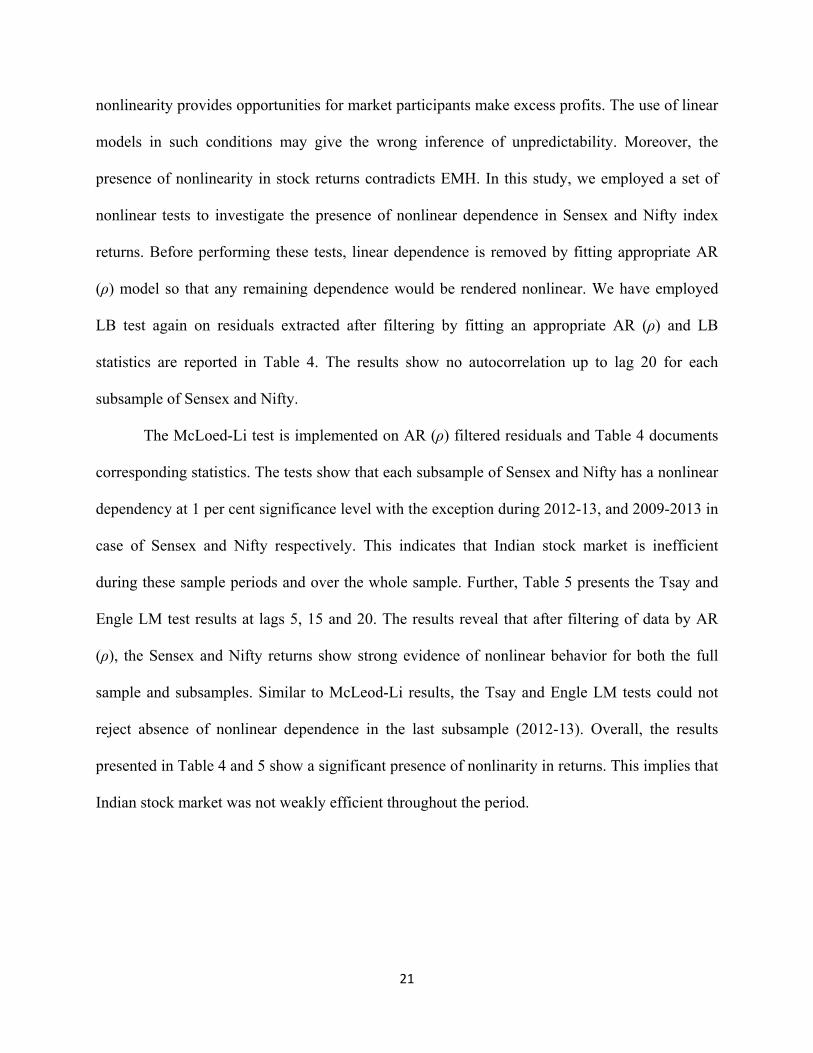
nonlinearity provides opportunities for market participants make excess profits. The use of linear
models in such conditions may give the wrong inference of unpredictability. Moreover, the
presence of nonlinearity in stock returns contradicts EMH. In this study, we employed a set of
nonlinear tests to investigate the presence of nonlinear dependence in Sensex and Nifty index
returns. Before performing these tests, linear dependence is removed by fitting appropriate AR
(ρ) model so that any remaining dependence would be rendered nonlinear. We have employed
LB test again on residuals extracted after filtering by fitting an appropriate AR (ρ) and LB
statistics are reported in Table 4. The results show no autocorrelation up to lag 20 for each
subsample of Sensex and Nifty.
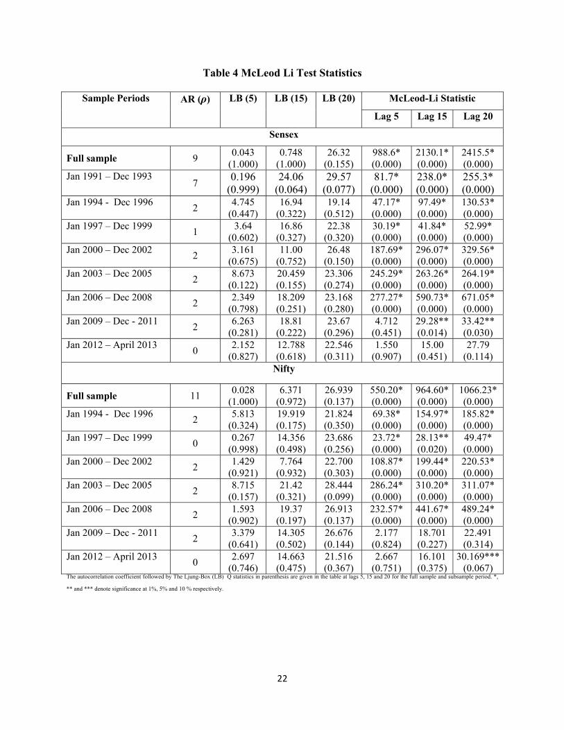
The McLoed-Li test is implemented on AR (ρ) filtered residuals and Table 4 documents
corresponding statistics. The tests show that each subsample of Sensex and Nifty has a nonlinear
dependency at 1 per cent significance level with the exception during 2012-13, and 2009-2013 in
case of Sensex and Nifty respectively. This indicates that Indian stock market is inefficient
during these sample periods and over the whole sample. Further, Table 5 presents the Tsay and
Engle LM test results at lags 5, 15 and 20. The results reveal that after filtering of data by AR
(ρ), the Sensex and Nifty returns show strong evidence of nonlinear behavior for both the full
sample and subsamples. Similar to McLeod-Li results, the Tsay and Engle LM tests could not
reject absence of nonlinear dependence in the last subsample (2012-13). Overall, the results
presented in Table 4 and 5 show a significant presence of nonlinarity in returns. This implies that
Indian stock market was not weakly efficient throughout the period.
22
Table 4 McLeod Li Test Statistics
Sample Periods AR (ρ) LB (5) LB (15) LB (20) McLeod-Li Statistic
Lag 5 Lag 15 Lag 20
Sensex
Full sample 9 0.043
(1.000)
0.748
(1.000)
26.32
(0.155)
988.6*
(0.000)
2130.1*
(0.000)
2415.5*
(0.000)
Jan 1991 – Dec 1993 7
0.196
(0.999)
24.06
(0.064)
29.57
(0.077)
81.7*
(0.000)
238.0*
(0.000)
255.3*
(0.000) Jan 1994 - Dec 1996
2 4.745
(0.447)
16.94
(0.322)
19.14
(0.512)
47.17*
(0.000)
97.49*
(0.000)
130.53*
(0.000)
Jan 1997 – Dec 1999 1
3.64
(0.602)
16.86
(0.327)
22.38
(0.320)
30.19*
(0.000)
41.84*
(0.000)
52.99*
(0.000)
Jan 2000 – Dec 2002 2
3.161
(0.675)
11.00
(0.752)
26.48
(0.150)
187.69*
(0.000)
296.07*
(0.000)
329.56*
(0.000)
Jan 2003 – Dec 2005 2
8.673
(0.122)
20.459
(0.155)
23.306
(0.274)
245.29*
(0.000)
263.26*
(0.000)
264.19*
(0.000)
Jan 2006 – Dec 2008 2
2.349
(0.798)
18.209
(0.251)
23.168
(0.280)
277.27*
(0.000)
590.73*
(0.000)
671.05*
(0.000)
Jan 2009 – Dec - 2011 2
6.263
(0.281)
18.81
(0.222)
23.67
(0.296)
4.712
(0.451)
29.28**
(0.014)
33.42**
(0.030)
Jan 2012 – April 2013 0
2.152
(0.827)
12.788
(0.618)
22.546
(0.311)
1.550
(0.907)
15.00
(0.451)
27.79
(0.114)
Nifty
Full sample 11 0.028
(1.000)
6.371
(0.972)
26.939
(0.137)
550.20*
(0.000)
964.60*
(0.000)
1066.23*
(0.000)
Jan 1994 - Dec 1996 2
5.813
(0.324)
19.919
(0.175)
21.824
(0.350)
69.38*
(0.000)
154.97*
(0.000)
185.82*
(0.000)
Jan 1997 – Dec 1999 0
0.267
(0.998)
14.356
(0.498)
23.686
(0.256)
23.72*
(0.000)
28.13**
(0.020)
49.47*
(0.000)
Jan 2000 – Dec 2002 2
1.429
(0.921)
7.764
(0.932)
22.700
(0.303)
108.87*
(0.000)
199.44*
(0.000)
220.53*
(0.000)
Jan 2003 – Dec 2005 2
8.715
(0.157)
21.42
(0.321)
28.444
(0.099)
286.24*
(0.000)
310.20*
(0.000)
311.07*
(0.000)
Jan 2006 – Dec 2008 2
1.593
(0.902)
19.37
(0.197)
26.913
(0.137)
232.57*
(0.000)
441.67*
(0.000)
489.24*
(0.000)
Jan 2009 – Dec - 2011 2
3.379
(0.641)
14.305
(0.502)
26.676
(0.144)
2.177
(0.824)
18.701
(0.227)
22.491
(0.314)
Jan 2012 – April 2013 0
2.697
(0.746)
14.663
(0.475)
21.516
(0.367)
2.667
(0.751)
16.101
(0.375)
30.169***
(0.067) The autocorrelation coefficient followed by The Ljung-Box (LB) Q statistics in parenthesis are given in the table at lags 5, 15 and 20 for the full sample and subsample period. *,
** and *** denote significance at 1%, 5% and 10 % respectively.

23
Table 5 Tsay, Engle LM and H Statistics
Sample Period
AR (ρ)
Tsay F Statistic Engle LM Statistic H Statistic
Lag 5 Lag 15 Lag 20 Lag 5 Lag 15 Lag 20
Sensex
Full sample 9
7.862*
(0.000)
3.613*
(0.000)
3.039*
(0.000)
564.1*
(0.000)
729.5*
(0.000)
758.2*
(0.000)
3760.9*
(0.000)
Jan 1991 – Dec 1993 7
2.837*
(0.000)
1.907*
(0.000)
1.786*
(0.000)
54.8*
(0.000)
101.2*
(0.000)
110.5*
(0.000)
405.6*
(0.000)
Jan 1994 - Dec 1996 2
1.858*
(0.000)
1.273**
(0.041)
1.282**
(0.016)
32.4*
(0.000)
50.5*
(0.000)
74.9*
(0.000)
139.7*
(0.000)
Jan 1997 – Dec 1999 1
2.436*
(0.001)
1.686*
(0.000)
1.457*
(0.000)
28.86*
(0.000)
37.5*
(0.001)
47.7*
(0.005)
183.9*
(0.000)
Jan 2000 – Dec 2002 2
2.396*
(0.002)
2.433*
(0.000)
2.168*
(0.000)
110.67*
(0.000)
138.8*
(0.000)
148.9*
(0.000)
364.8*
(0.000)
Jan 2003 – Dec 2005 2
6.609*
(0.000)
2.257*
(0.000)
1.910*
(0.000)
268.96*
(0.000)
272.2*
(0.000)
272.3*
(0.000)
721.7*
(0.000)
Jan 2006 – Dec 2008 2
4.734*
(0.000)
2.746*
(0.000)
2.667*
(0.000)
153.7*
(0.000)
179.4*
(0.000)
181.7*
(0.000)
680.9*
(0.000)
Jan 2009 – Dec - 2011 1
1.24
(0.229)
2.50*
(0.000)
2.483*
(0.000)
4.9
(0.495)
22.8
(0.088)
24.3
(0.231)
242.9*
(0.000)
Jan 2012 – April 2013 0
0.560
(0.903)
1.558*
(0.003)
1.073
(0.359)
1.6
(0.911)
13.3
(0.576)
25.8
(0.172)
52.8
(0.198)
Nifty
Full sample 9 6.240*
(0.000)
2.877*
(0.000)
2.427*
(0.000)
352.20*
(0.000)
425.36
(0.000)
437.38*
(0.000)
1848.41*
(0.000) Jan 1994 - Dec 1996
2 1.509
(0.095)
1.583*
(0.000)
1.436*
(0.000)
50.21*
(0.000)
77.758
(0.000)
92.62*
(0.000)
158.67*
(0.000)
Jan 1997 – Dec 1999 0
2.842*
(0.000)
1.687*
(0.000)
1.295**
(0.011)
24.21*
(0.000)
27.85**
(0.022)
51.658*
(0.000)
157.77*
(0.000)
Jan 2000 – Dec 2002 2
1.852**
(0.024)
2.173*
(0.000)
1.949*
(0.000)
79.97*
(0.000)
126.46*
(0.000)
130.54*
(0.000)
380.80*
(0.000)
Jan 2003 – Dec 2005 2
6.757*
(0.000)
2.413*
(0.000)
1.985*
(0.000)
315.46*
(0.000)
320.34*
(0.000)
321.86*
(0.000) 799.69*
(0.000) Jan 2006 – Dec 2008
2 5.583*
(0.000)
2.705*
(0.000)
2.459*
(0.000)
125.40*
(0.000)
152.41*
(0.000)
158.98*
(0.000)
663.08*
(0.000)
Jan 2009 – Dec - 2011 2
0.873
(0.593)
2.313*
(0.000)
2.268*
(0.000)
2.023
(0.845)
15.292
(0.430)
16.87
(0.661)
195.63*
(0.000)
Jan 2012 – April 2013 2
0.489
(0.945)
1.577*
(0.003)
1.181
(0.193)
2.931
(0.710)
14.672
(0.475)
27.786
(0.114)
56.255
(0.121) *,** denote 1 % and 5 % significance level.

24
The Hinich bicorrelation (H) tests the null of pure noise. The H statistics presented in
Table 5 reveal that with the exception of subsample 2012-2013, the null of pure noise is clearly
rejected for Sensex and Nifty returns at 1 percent level of significance. The inference drawn is
that nonlinearity characterizes the Indian stock returns and hence returns are predictable . In
short, the results documented in Table 5 show strong evidence of nonlinear dependence in
returns indicating Indian stock market is inefficient during the full sample period and sub-periods
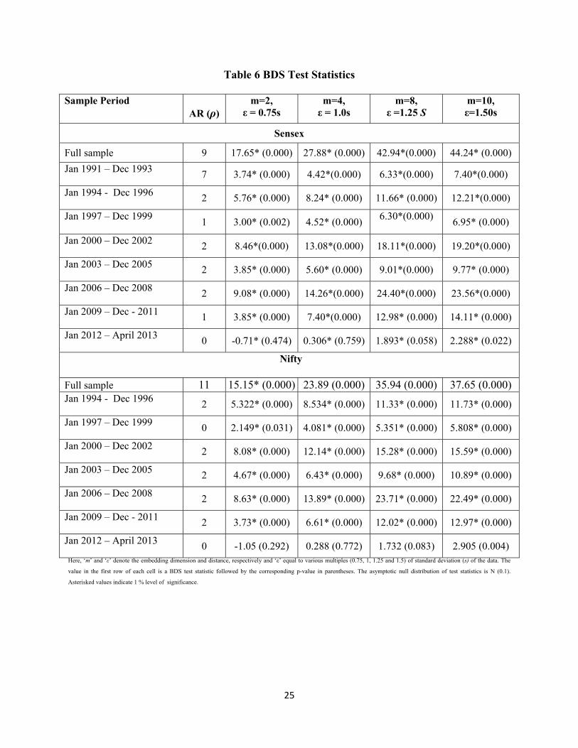
as well. Finally, the BDS test is performed at various embedded dimensions (m) like 2, 4, and 8
and 10 at various distances (ε) like 0.75s, 1.0s, 1.25s and 1.50s where s denotes standard
deviations of the return. It is clear from the BDS statistics in Table 6 that all the subsamples and
full sample reject the null for both the indices. The rejection for residuals from AR (ρ) indicates
presence of nonlinear dependence in the Sensex and Nifty returns series implying the possible
predictability of future returns using the history of returns. This invalidates EMH in case of
Indian stock market.
To comprehend the magnitude of nonlinear dependence, Fig. 2 plots the nonlinear test
statistics. The McLeod-Li results show stronger presence of nonlinear dependence in Sensex and
Nifty returns during subsamples 2003-2005 and 2006-2008. Again, the trends in Engle LM,
Tsay, H and BDS test statistics are low indicating lesser magnitude of nonlinear dependency
again both in Sensex and Nifty returns up to 2000 and thereafter returns exhibit increasing
nonlinear tendency reaching peak during subsample, 2006-2008. However, in post 2008
subsample, all the test statistics are less significant suggesting weaker presence of nonlinear
dependence in returns.
25
Table 6 BDS Test Statistics
Sample Period
AR (ρ)
m=2,
ε = 0.75s
m=4,
ε = 1.0s
m=8,
ε =1.25 S
m=10,
ε=1.50s
Sensex
Full sample 9 17.65* (0.000) 27.88* (0.000) 42.94*(0.000) 44.24* (0.000)
Jan 1991 – Dec 1993 7 3.74* (0.000) 4.42*(0.000) 6.33*(0.000) 7.40*(0.000)
Jan 1994 - Dec 1996 2 5.76* (0.000) 8.24* (0.000) 11.66* (0.000) 12.21*(0.000)
Jan 1997 – Dec 1999 1 3.00* (0.002) 4.52* (0.000)
6.30*(0.000)
6.95* (0.000)
Jan 2000 – Dec 2002 2 8.46*(0.000) 13.08*(0.000) 18.11*(0.000) 19.20*(0.000)
Jan 2003 – Dec 2005 2 3.85* (0.000) 5.60* (0.000) 9.01*(0.000) 9.77* (0.000)
Jan 2006 – Dec 2008 2 9.08* (0.000) 14.26*(0.000) 24.40*(0.000) 23.56*(0.000)
Jan 2009 – Dec - 2011 1 3.85* (0.000) 7.40*(0.000) 12.98* (0.000) 14.11* (0.000)
Jan 2012 – April 2013 0 -0.71* (0.474) 0.306* (0.759) 1.893* (0.058) 2.288* (0.022)
Nifty
Full sample 11 15.15* (0.000) 23.89 (0.000) 35.94 (0.000) 37.65 (0.000)
Jan 1994 - Dec 1996 2 5.322* (0.000) 8.534* (0.000) 11.33* (0.000) 11.73* (0.000)
Jan 1997 – Dec 1999 0 2.149* (0.031) 4.081* (0.000) 5.351* (0.000) 5.808* (0.000)
Jan 2000 – Dec 2002 2 8.08* (0.000) 12.14* (0.000) 15.28* (0.000) 15.59* (0.000)
Jan 2003 – Dec 2005 2 4.67* (0.000) 6.43* (0.000) 9.68* (0.000) 10.89* (0.000)
Jan 2006 – Dec 2008 2 8.63* (0.000) 13.89* (0.000) 23.71* (0.000) 22.49* (0.000)
Jan 2009 – Dec - 2011 2 3.73* (0.000) 6.61* (0.000) 12.02* (0.000) 12.97* (0.000)
Jan 2012 – April 2013 0 -1.05 (0.292) 0.288 (0.772) 1.732 (0.083) 2.905 (0.004)
Here, ‘m’ and ‘ε’ denote the embedding dimension and distance, respectively and ‘ε’ equal to various multiples (0.75, 1, 1.25 and 1.5) of standard deviation (s) of the data. The
value in the first row of each cell is a BDS test statistic followed by the corresponding p-value in parentheses. The asymptotic null distribution of test statistics is N (0.1).
Asterisked values indicate 1 % level of significance.

26
Fig. 2 Trends in Nonlinear Test Statistics
The present evidence of the strong presence of nonlinear dependence throughout the
sample, and highest during periods financial crashes are consistent with the findings of Urquhart
and Hudson (2013) who found similar evidence in the case of the US market. The inference from
Fig. 2 is that during the sample period of the study, there has been increasing presence of
1994-99 1997-99 2000-02 2003-05 2006-08 2009-11 2012-13 0
100
200
300
400
500
700
800
-2
0
2
4
6
8
10MCLEODLI ENGLELM HSTATISTIC TSAY BDS
1991-93 1994-96 1997-99 2000-02 2003-05 2006-08 2009-11 2012-13 0
100
200
300
400
500
600
700
800
-2
0
2
4
6
8
10MCLEODLI ENGLELM HSTATISTIC
TSAY BDS
27
nonlinear dependence with a sign of the declining magnitude of nonlinear dependence in Indian
stock returns from 2009. The subsample 2006-2008, which possess strong pockets of nonlinear
dependence is associated with sub-prime mortgage and global financial crisis. Overall, there is
strong evidence of nonlinearity throughout the sample period in Indian market. Although we find
evidence of an increasing nonlinear dependence, it is tapering in most recent subsamples.
5. Summary and conclusion
The present paper has investigated the adaptive market hypothesis (AMH) in emerging
markets like India. To validate the issue empirically, we employed linear and nonlinear tests over
the whole sample from 1991 to 2013 and on subsamples of two years each. The linear test LB Q
and runs test results indicate a cyclical pattern in autocorrelations suggesting that the Indian
stock market switched between periods of efficiency and inefficiency. The variance ratio tests
find dependence only during the full sample period and independence of returns in each
subsample. The findings also suggest unpredictability of returns during crisis periods. This
shows that Indian stock market is efficient barring few brief periods of predictability, which
quickly disappear as information starts reflecting in prices.
The failure in rejecting linear dependence is not sufficient to prove independence because
of possibility of presence of nonlinearity in returns, which indicate predictability and consequent
abnormal profits to the agents. To test such possibilities, we employed a set of nonlinear tests.
The findings from each of the tests suggest that there is a strong presence of nonlinear
dependence in Indian stock returns implying possible predictability of returns and consequent
excess returns. Moreover, the results have shown that there was a strong presence of nonlinear
dependence during periods of crisis in 1997-99 and 2006-2008 thus suggesting better

28
predictability of returns during periods of crashes. The present evidence of nonlinearity in returns
straight away reject the efficient market hypothesis in the case of India.
The findings of the present study do not suggest that Indian stock market is not fully
adaptive, as it has not gone through at least three different stages of dependency required under
AMH framework. However, linear test results indicate that Indian stock market has gone through
periods of efficiency and inefficiency and, the magnitude of nonlinear dependence has declined
in recent periods which is suffice it to conclude that Indian stock market is in the first stage of
AMH. This implies that the reforms initiated have not fully brought the desired results. The
evidence necessitates active portfolio management for generating excess returns. In light of the
nonlinear dependence in returns, it is useful to use nonlinear methods for better forecasts. The
present finding of an increased possibility of predictability during crashes call for appropriate
policy measure to make the market immune to the ill effects of external events.

29
References
Alvarez-Ramirez, J., Rodriguez E., Espinosa-Paredes, G.: Is the US stock market becoming
weakly efficient over time? Evidence from 80-year-long data. Phys A. 391,5643-5647 (2012)
Amanulla, S., Kamaiah, B.: Indian stock market: Is it informationally efficient? Prajnan. 25, 473-
485(1998)
Bachelier, L.: Theory of Speculation. PhD Thesis, Faculty of the Academy of Paris (1900)
Barua, S.K.: The short run price behaviour of securities: Some evidence on efficiency of Indian
capital market. Vikalpa. 16,93-100 (1981)
Brock, W.A., Sheinkman, J.A., Dechert, W.D., LeBaron, B.: A test for independence based on
the correlation dimension. Econom Rev. 15,197–235 (1996)
Campbell, J.Y., Lo, A.W., MacKinlay, A.C.: The Econometrics of financial markets. Princeton,
New Jersey (1997)
Charles, A., Darne, O., Kim, H.: Exchange-rate predictability and adaptive market hypothesis:
Evidence from major exchange rates. J Int Money Financ. 31,1607-1626 (2012)
Chow, K.V., Denning, K.C.: A simple multiple variance ratio test. J Econom. 58:385-401 (1993)
Engle, R.F.: Autoregressive conditional heteroskedasticity with estimates of the variance of
United Kingdom inflation. Econom. 50, 987-1007 (1982)
Fama, E.F.: Efficient capital markets: A review of theory and empirical work. J Financ. 25, 383-
417 (1970)
Granger, C.W.J., Anderson, A.P.: An introduction to bilinear time series models. V & R,
Gottingen (1978)
Grassberger, P., Procaccia, I.: Characterization of strange attractors. Phys Rev Lett. 50, 346-340
(1983)
Hsieh, D.A.: Testing for nonlinear dependence in daily foreign exchange rates. J Buss. 62 (3):
339-368 (1989)
Hinich, M.J.: Testing for dependence in the input to a linear time series model. J Non-paramet
Stat. 6, 205-221(1996)
Ito, M., Sugiyama, S.: Measuring the degree of time varying market inefficiency. Econ Lett. 103,
62–64 (2009)
Jarque, C.M., Bera, A.K.: Efficient test of normality, homoscedasticity and serial independence
of regression residuals. Econ Lett. 6, 255-259 (1980)

30
Kim, J.H., Shamsuddin, A., Lim, K.P.: Stock returns predictability and the adaptive markets
hypothesis. Evidence from century long U.S. data. J Empiri Financ. 18, 868-879 (2011)
Ljung, G.M., Box, G.E.P.: On a measure of lack of fit in time series models. Biom. 65, 297-303
(1978)
Lo, A.W.: The adaptive markets hypothesis: market efficiency from an evolutionary perspective.
J Portf Manag. 30, 15–29 (2004)
Lo, A.W.: Reconciling efficient markets with behavioral finance: The adaptive markets
hypothesis. J Invest Consult. 7, 21–44 (2005)
Lo, A.W., MacKinlay, A.C.: Stock market prices do not follow random walks: Evidence from a
simple specification test. Rev Financ Studies. 1, 41-66 (1988)
Lo, A.W., MacKinlay, A.C.: A non-random walk down Wall Street. Princeton, New Jersey
(1999)
Malkiel, B.G.: A random walk down Wall Street. W. W. Norton & Co, New York (1973)
McLeod, A.I., Li, W.K.: Diagnostic checking ARMA time series models using squared-residual
autocorrelations. J Time Ser Anal. 4, 269-273 (1983)
Noda, A.: A test of the adaptive market hypothesis using non-Bayesian time-varying AR model
in Japan. http://arxiv.org/abs/1207.1842 (2012). Accessed on 25 January 2013
Poshakwale ,S.: The random walk hypothesis in the emerging Indian stock market. Journal of
Bus Financ & Account. 29, 1275-1299
Rao, K.N., Mukherjee, K.: Random walk hypothesis: An empirical study. Arthaniti. 14, 53-58
(1971)
Samuelson, P.: Proof that properly anticipated prices fluctuate randomly. Ind Manag Rev. 6. 41-
49 (1965)
Sharma, J.L., Kennedy, R.E.: A comparative analysis of stock price behavior on the Bombay,
London, and New York stock exchanges. J Financ Quant Analysis. 12, 391-413 (1977)
Siegel, S.: Nonparametric statistics for behavioral Sciences. McGraw-Hill, New York (1956)
Standard and Poor’s.: Global stock market fact book, New York(2012)
Tsay, R.S.: Nonlinearity tests for time series. Biom. 73:461-466 (1986)
Taylor, S.J.: Asset price dynamics, volatility, and prediction. Princeton, New Jersey (2005)

31
Urquhart, A., Hudson, R.: Efficient or adaptive markets? Evidence from major stock markets
using very long historic data. Int Rev Financ Anal. 28,130-142 (2013)