arX

iv:2

111.

1319

1v2

[ph

ysic

s.so

c-ph

] 9

Dec

202

1

Analysis of emergent patterns in crossing flows of pedestriansreveals an invariant of ‘stripe’ formation in human data

Pratik Mullick1*, Sylvain Fontaine2¤, Cecile Appert-Rolland2, Anne-Helene Olivier3,William H. Warren4, Julien Pettre1

1 INRIA Rennes - Bretagne Atlantique, Campus de Beaulieu, Rennes, France2 Universite Paris-Saclay, CNRS/IN2P3, IJCLab, Orsay, France3 Universite Rennes, INRIA, CNRS, IRISA, M2S, France4 Department of Cognitive, Linguistic and Psychological Sciences, Brown University,Providence, Rhode Island, USA

¤Current Address: Sorbonne Universite, CNRS - GEMASS, Paris, France* pratik.mullick@inria.fr

Abstract

When two streams of pedestrians cross at an angle, striped patterns spontaneouslyemerge as a result of local pedestrian interactions. This clear case of self-organizedpattern formation remains to be elucidated. In counterflows, with a crossing angleof 180°, alternating lanes of traffic are commonly observed moving in opposite direc-tions, whereas in crossing flows at an angle of 90°, diagonal stripes have been reported.Naka (1977) hypothesized that stripe orientation is perpendicular to the bisector of thecrossing angle. However, studies of crossing flows at acute and obtuse angles remain un-derdeveloped. We tested the bisector hypothesis in experiments on small groups (18-19participants each) crossing at seven angles (30° intervals), and analyzed the geometricproperties of stripes. We present two novel computational methods for analyzing stripedpatterns in pedestrian data: (i) an edge-cutting algorithm, which detects the dynamicformation of stripes and allows us to measure local properties of individual stripes; and(ii) a pattern-matching technique, based on the Gabor function, which allows us to esti-mate global properties (orientation and wavelength) of the striped pattern at a time T .We find an invariant property: stripes in the two groups are parallel and perpendicularto the bisector at all crossing angles. In contrast, other properties depend on the cross-ing angle: stripe spacing (wavelength), stripe size (number of pedestrians per stripe),and crossing time all decrease as the crossing angle increases from 30° to 180°, whereasthe number of stripes increases with crossing angle. We also observe that the width ofindividual stripes is dynamically squeezed as the two groups cross each other. The find-ings thus support the bisector hypothesis at a wide range of crossing angles, althoughthe theoretical reasons for this invariant remain unclear. The present results provideempirical constraints on theoretical studies and computational models of crossing flows.

Author summary

You may have noticed that pedestrians in a crosswalk often form multiple lanes oftraffic, moving in opposite directions (180°). Such spontaneous pattern formation isan example of self-organized collective behavior, a topic of intense interdisciplinaryinterest. When two groups of pedestrians cross at an intersection (90°), similar diagonal

December 10, 2021 1/33

stripes appear. Naka (1977) conjectured that the stripes are perpendicular to the meanwalking direction of the two groups. This facilitates the forward motion of each groupand reduces collisions. We present the first empirical test of the hypothesis by studyingtwo groups of participants crossing at seven different angles (30° intervals). To analyzethe striped patterns, we introduce two computational methods, a local Edge-cuttingalgorithm and a global Pattern-matching technique. We find that stripes are indeedperpendicular to the mean walking direction at all crossing angles, consistent with thehypothesis. But other properties depend on the crossing angle: the number of stripesincreases with crossing angle, whereas the spacing of stripes, the number of pedestriansper stripe, and the crossing time all decrease. Moreover, the width of individual stripesis “squeezed” in the middle of the crossing. Future models of crowd dynamics will needto capture these properties.

Introduction

Collective motion in groups of humans, as well as other social organisms, has increasinglybecome a subject of analysis and modeling [1–7]. Currently, characteristic patterns ofcollective motion are understood as emergent behavior resulting from the collectivedynamics of interactions between individuals. Studies of human crowd dynamics haveimportant applications to improving pedestrian traffic flow, safety management, and theprevention of crowd disasters [8–12]. Analyses of real-life mass events have been used tomodel crowd behavior in situations such as religious gatherings, rock concerts, sportingmatches, and transportation hubs [13–16], with a critical goal of averting life-threateningcrushes, stampedes, and trampling [14, 17, 18]. A first step to successful modeling isa better understanding of actual crowd behavior by analysis of crowd dynamics andpattern formation in human data. In this paper, we develop a computational analysisof spontaneous stripe formation in crossing flows of pedestrians.

Pedestrian traffic flow has been studied empirically in a wide variety of situations,using both experimental methods and motion tracking of real crowds. The simplestcase is uni-directional flow in a corridor, in which properties such as the dependence ofspeed on density have been analyzed [19–24]. Collision avoidance between pedestrianshas been investigated in pairs of walkers [25,26] and multiple walkers [27]. Bottlenecksoccur when a large group attempts to pass through a narrow opening [21, 28–33], as inBlack Friday sales or fire emergencies, which can lead to jamming and crushes. Otherempirical studies have examined pedestrian flow through a T-junction [34, 35], multi-directional flows [36], a pedestrian crossing through a dense static crowd [37,38], and abottleneck leading to a 1D corridor [39].

Crossing flows can be described as two streams of pedestrians walking in differentdirections, passing through each other at a crossing angle α > 0° (where 0° is walking inthe same direction). Many real-world situations produce crossing flows, such as streamsof pedestrians crossing at a sidewalk intersection, or subway commuters passing eachother when entering and exiting a metro car. A special case of crossing flows, calledcounterflow, occurs when the crossing angle is 180°. Self-organized spatial patternshave been observed when two groups cross each other. In counterflow, the formation ofstable lanes is regularly reported in both human experiments [3,36,40–44] and numericalsimulations [45–57], in which alternating lanes of pedestrian traffic are aligned with thewalking directions of the two groups (180° apart). A jamming transition can occurabove a critical flow density [47,51,54,55]. More generally, at other crossing angles theformation of stripes is observed, but the alternating stripes are not aligned with thewalking directions of the two groups. The familiar case of orthogonal flows (α = 90°)has been widely studied, and the formation of diagonal stripes is found in human crowds[53, 58] and in simulation [40, 52, 53, 59–64]. However, the analysis of crossing flows in

December 10, 2021 2/33

humans at other crossing angles remains underdeveloped.Naka [58] first reported stripes at acute and obtuse crossing angles in pedestrian

crowds, and hypothesized that stripes form at an orientation that is perpendicular tothe bisector of the crossing angle. Abstractly, a stripe is a traveling wave that movesin the mean direction of the two flows, such that individual pedestrians travel forwardwith a stripe and laterally within it [41]. A striped pattern facilitates overall pedestrianflow by reducing collision-avoidance maneuvers, thereby increasing the average walkingspeed. Only one subsequent human study [65] has tested oblique crossing angles (45°and 135°), but stripe patterns were not analyzed. The bisector hypothesis thus remainsto be tested experimentally.

Striped patterns in oblique crossing flows have been reproduced in simulation, con-sistent with the bisector hypothesis [41]. In one system, the inclination of the stripe tothe bisector was found to increase with the velocity difference between two orthogonalflows [52]. The mechanism responsible for the formation of self-organized stripes in or-thogonal flows has been studied theoretically [61–64]. A mean field analysis shows theunderlying mechanism to be a linear instability of the randomly uniform state in theintersecting region compared to the formation of diagonal striped patterns [61, 63, 64].The ‘wake’ of a pedestrian has been proposed as the microscopic mechanism for stripeformation, a density perturbation created in the perpendicularly moving flow [62]. Theinclination of the striped patterns was related to the velocity difference between the twogroups, producing a ‘chevron’ effect [61, 63]. Absence of striped patterns has also beenobserved when three or more groups of people intersect [66–68].

The purpose of the present research is to experimentally test the bisector hypothesisby analyzing stripe formation at a variety of crossing angles, without spatial constraints.We seek to answer several theoretically-motivated questions: (i) Can stripe orientationbe predicted as perpendicular to the bisector for all crossing angles? (ii) Do other stripeproperties depend on crossing angle? (iii) What are the stripe dynamics during crossingflows? (iv) Does spontaneous stripe formation generalize from continuous crossing flowsin defined corridors to small crowds without boundary conditions on spatial position,density, or visibility?

We addressed these questions as part of the PEDINTERACT Project [37], in whichtwo different sets of subjects participated (36 on Day 1, 38 on Day 2). The setup appearsin Fig 1 (also see S1 Video). In the experiment, two groups of participants (18 or 19 pergroup) walked through each other at seven different crossing angles (0° to 180°, at 30°intervals); there were approximately 17 trials per angle. On each trial, the groups werepositioned in two starting boxes oriented at the designated crossing angle, and wereinstructed to walk in the direction they were facing to the other side of the room. Toinvestigate whether striped patterns would emerge in the absence of spatial boundaryconditions, we did not use opaque corridors as in many previous studies [41, 59, 61, 65].Head position was recorded with a motion-capture system at 120 Hz. Sample traces forall pedestrians in a typical trial appear in Fig 2.

Because the empirical analysis of crossing flows is quite underdeveloped, we describea number of computational methods for analyzing the characteristics of stripes in humandata. In particular, we present a novel approach to identify the formation of stripes,called the Edge-cutting algorithm. Using this algorithm we were able to measure thelocal properties of individual stripes such as their orientation, width and size. We alsouse an independent method to characterize global stripe properties, a pattern match-ing technique that fits a two dimensional sinusoidal function (e.g. Gabor function) tothe positions of pedestrians in the two groups. This method assumes the existence ofa periodic pattern of stripes and then finds the geometric properties of the patternfrom a fitting procedure. The two methods are complementary, in the sense that theedge-cutting algorithm requires the whole history of the crossing and provides the full

December 10, 2021 3/33

Fig 1. Photograph of our experimental set-up to study crossing flows. Agents participating in ourexperiment are shown in this photograph for a typical trial with crossing angle 120°. The three stages of the trial areshown here, viz. (a) before crossing (b) during crossing and (c) after crossing.

-10

-5

0

5

10

-10 -5 0 5 10

time = T1

y [

m]

x [m]

-10

-5

0

5

10

-10 -5 0 5 10

time = T2

T1 < T2 < T3

y [

m]

x [m]

-10

-5

0

5

10

-10 -5 0 5 10

time = T3

y [

m]

x [m]

Fig 2. Illustration of a trial of crossing flow from our experiments. Traces of all the pedestrians involved for atypical trial has been shown with expected value of crossing angle equal to 60°. Three different instances of the trial hasbeen shown here viz. before crossing (T1), during crossing (T2) and after crossing (T3). The actual values of timeframes are T1 = 2.3 sec, T2 = 6.55 sec and T3 = 10.8 sec from the beginning of the trial. The two groups of pedestriansare denoted by blue and red dots. The tails behind each of the dots are basically the distances travelled by thepedestrians in previous 1.25 sec.

dynamics of the stripes, whereas the pattern matching method can be performed ona single snapshot. The stripe orientations obtained by the edge-cutting algorithm andthe pattern matching technique are compared to each other, and to the hypothesis thatthe stripes are perpendicular to the bisector of the crossing angle.

In sum, the present paper makes two major contributions: (i) we present experimen-tal data on crossing flows of pedestrians that support the bisector hypothesis, and (ii)we introduce and discuss methodological tools to detect the formation and presence ofstriped patterns and to estimate their geometric properties.

Results

When two groups of people cross each other, striped patterns emerge, as schematicallyillustrated in Fig 3. The primary goal of the present research was to characterizethe properties of these emergent stripes, based on numerical analysis of participant

December 10, 2021 4/33

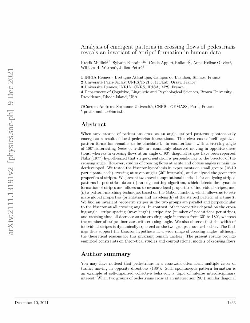
trajectories. The actual crossing angle α between the mean walking directions of thetwo groups was measured from the data. The properties of stripe orientation γ relativeto the crossing angle bisector, and stripe spacing λ are illustrated in Fig 3 (right). Webegin by introducing two independent computational methods devised to analyze thegeometric properties of the stripes, (i) the Edge-cutting algorithm and (ii) the Pattern-matching technique.

time = T1 2 3

T < T < T1 2 3

time = T time = T

γ

γ

λ

λα

Fig 3. Schematic representation for the formation of stripes and definition of orientation γ and physicalseparation λ of stripes. Formation of stripes as a consequence of two groups crossing each other. In this schematicdiagram the crossing angle between the two groups is α. The figure has been shown for three instances viz. beforecrossing (T1), during crossing (T2) and after crossing (T3). The two groups before crossing are denoted by blue and redsquares, whose direction of motion is denoted by arrows of the same color. The green dotted arrow denotes the bisectorof the crossing angle. The orientation γ of the stripes is measured counter-clockwise from the bisector. λ is the spatialseparation between two stripes from the same group. For specific definitions of γ and λ see Fig 6.

Identifying stripes using edge-cutting algorithm

For purposes of the first method, we define a stripe as a subset of participants fromone group that is not penetrated by participants from the other group. Specifically,the virtual connections or edges between the participants in a stripe are never crossedor ‘cut’ by the trajectory of a participant from the other group. The principal outputof the Edge-cutting algorithm is the identification of the participants who belong toeach stripe (see Materials and Method for details). This analysis indeed revealed thespontaneous emergence of striped patterns and the stripes were successfully identified.The dynamics of stripe formation was also observed, as illustrated for two typical trialsin Fig 4. The Edge-cutting algorithm also yields the time of the initial edge-cut Ti atthe start of crossing (left column of Fig 4) and the time of the final edge-cut Tf at theend of crossing (right column of Fig 4). Animations of the Edge-cutting process forthese two trials appear in the supplementary material (S2 Video and S3 Video).

Characterizing stripes using pattern-matching technique

The Pattern-matching technique estimates the orientation and width of a set of stripes,assuming that the stripes are parallel and equally spaced. This method fits a two-dimensional spatial frequency function f , based on a sinusoidal Gabor function, to the

December 10, 2021 5/33

-10

-5

0

5

10

-10 -5 0 5 10

time = Ti

α =

116.9

°

y [

m]

x [m]

-10

-5

0

5

10

-10 -5 0 5 10

time = Tf

y [

m]

x [m]

-10

-5

0

5

10

-10 -5 0 5 10

time = (Ti + Tf)/2

y [

m]

x [m]

-10

-5

0

5

10

-10 -5 0 5 10

time = Ti

α =

89.8

°

y [

m]

x [m]

-10

-5

0

5

10

-10 -5 0 5 10

time = Tf

y [

m]

x [m]

-10

-5

0

5

10

-10 -5 0 5 10

time = (Ti + Tf)/2

y [

m]

x [m]

Fig 4. Pictorial representation of the edge-cutting algorithm. Figure demonstrates the working process of theedge-cutting algorithm as a sequence of time. Here we show the process for two typical trials with α = 89.8° andα = 116.9°. Red and blue arrows indicate the direction of motion of the two groups represented by red and blue dotsrespectively. The lines connecting the dots in each of the groups are considered as the virtual bonds or ‘edges’ whichare suppressed when cut by a pedestrian on the other group (see Materials and Methods). The figures are shown forthree instances, viz. Ti, (Ti + Tf )/2 and Tf . Ti and Tf denote the instances of time when the first and last edge-cuttake place respectively. The edge-cutting process for the entire course of time for these two trials are shown as videos insupplementary materials (S2 Video and S3 Video).

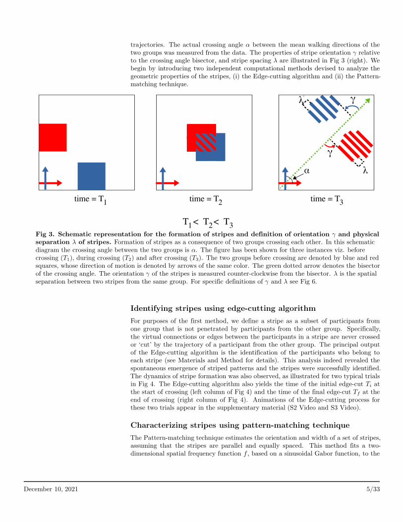
positions of pedestrians at a time T . The free parameters of orientation γ, wavelength λ,and phase ψ, are chosen by maximizing C, the fit of the function to pedestrian positions,where positive values (peaks) are assigned to one group and negative values (troughs)to the other (see Materials and Methods for details). The fitting can be applied to allpedestrians or to a subset (e.g. one group). The output of this fitting procedure forall pedestrians in two representative trials appears in Fig 5, where γ and λ refer to theorientation and wavelength of stripes in the whole crowd.

The two methods are complementary. The edge-cutting algorithm requires the wholehistory of the crossing event and yields in return the full dynamics of stripes. It estimatesthe local spatial properties of individual stripes at each time point, without assumingany prior knowledge about them. The pattern-matching technique requires only a singlesnapshot, and recovers the global spatial properties of orientation and wavelength. Theprior assumptions of parallel, equally spaced stripes help to match the instantaneouspattern, as long as the actual stripes are close to this ideal. We will see now how bothapproaches allow us to gain insight into the striped structure.

December 10, 2021 6/33

Fig 5. Output of the pattern matching technique. The panels on the left show fitting of pedestrian positions forthe same trials shown in Fig 4. Fitting was done using the parametric sine curve f and the transformed coordinates(x′, y′). The blue and red parts of the plot represent the crests and troughs of the sine function respectively. Theoutputs of the fitting are γ = 83.34°, λ = 1.865m and ψ = −116.37° for the typical trial with α = 89.8° and γ = 89.99°,λ = 2.286m and ψ = −0.92° for the typical trial with α = 116.9°. (see Materials and Methods) The panels on the rightshow variation of C as a function of γ and λ keeping ψ fixed to the value obtained from the fitting shown in the leftpanel. The region of occurrence of high values of C is shown in yellow. The function C was maximised to fit the sinefunction f . The maximum value of C for the trial with α = 89.8, as obtained by our optimisation procedure is 1.132,which occurred for γ = 83.34° and λ = 1.865m. Whereas, for the trial with α = 116.9° we obtained the maximum valueof C = 1.205, which occurred for γ = 89.99° and λ = 2.286m.

Stripe Orientation

Based on previous empirical observations and modeling, there are reasons to expect thatthe observed stripes would be parallel and perpendicular to the bisector of the crossingangle, as illustrated in Fig 3. This bisector hypothesis thus predicts γ = 90° for allcrossing angles α. However, it is possible that the stripes for one group (blue in Fig3) are not parallel to those for the other group (red), such that γblue 6= γred; also thatindividual stripes within a group are not parallel. We thus estimated the orientation ofstripes using the global and local methods: (i) the Pattern-matching technique allowedus to estimate the overall stripe orientation γ (Fig 6a), as well as the orientation foreach group separately γL and γL, (Fig 6b); (ii) the Edge-cutting algorithm enabled usto estimate the orientation of individual stripes γL and γR, (Fig 6c). We report each of

December 10, 2021 7/33

these measurements of stripe orientation in turn.

λ�

γ�

α α α

γ

γ

~

~

L

R

Lγ

γR

λL~

~λR

(a) (b) (c)

Estimated fromEdge-cutting Algorithm

Estimated fromparametric sinusoidal fitting

Fig 6. Summary of different methods to estimate orientation γ and physical separation λ of the stripes.The arrows in blue and red represents the direction of motion of the two groups. The schematic diagrams are shown foran arbitrary crossing angle. The dashed green arrow indicates the bisector of the crossing angle between the two groupdirection vectors. The lines in blue and red show the stripes from the two groups. γ is the angle between the directionof stripes and the bisector of crossing angle, always measured counterclockwise. (a) Estimation of orientation γ of thestripes and physical separation λ between two stripes from the same group using the parametric sinusoidal fitting. Indoing this calculation it was assumed that stripes from the two groups are parallel to each other and are equispaced, asshown in the figure. (b) Orientation of the stripes from the two groups when we assume that stripes from the samegroup are parallel to each other and are equispaced. γL and γR denote the orientation of stripes whose group directionvectors are left and right to the direction of bisector respectively. Using the same convention, γL and γR are the spatialseparation between the stripes in those cases. This calculation was also done by fitting the two dimensional sine curve.(c) Estimation of orientation of the individual stripes that were found using the edge-cutting algorithm, for the twogroups. γL or γR denote the orientation of individual stripes whose group direction vector is left or right to thedirection of bisector respectively.

Global stripe orientation γ and γ using the Pattern-matching technique

In the first analysis, we estimated the overall orientation of all stripes γ to the bisector,on the assumption that the stripes for the two groups were parallel and equally spaced(see Fig 6a), using the pattern matching technique. The analysis was performed at asuitable time T between the crossing midpoint (Ti + Tf)/2 and the final crossing pointTf , when the periodic pattern of stripes was most clearly defined (see Discussion). Theresulting values of γ are represented in box plots in Fig 7a (blue bars). Note that themedian values are very close to the predicted angle of 90° for all crossing angles, withdeviations less than 3° in all conditions. A set of t-tests comparing the mean value of γ to90° at each crossing angle was significant only for α = 63.8°, t(17) = −2.550, p = 0.0207;no other conditions were significant. Overall, this finding is consistent with the bisectorhypothesis. A one-way analysis of variance (ANOVA) on γ was also performed, withcrossing angle α as the factor (excluding the 0° condition). The result found that stripeorientation did not depend significantly on crossing angle, F (5, 99) = 2.301, p = 0.0504,η2 = 0.1.

December 10, 2021 8/33

40

60

80

100

120

140

160

26.1 63.8 89.8 116.9 154.1 179.7

(a)_

*

ori

enta

tio

n o

f st

rip

es b

y d

iffe

ren

t m

eth

od

s [°

]

crossing angle α [°]

γγ~L

γ~RγL

γR

-40

-20

0

20

40

26.1 63.8 89.8 116.9 154.1 179.7

(b)

dif

fere

nce

in o

rien

tati

on o

f st

ripes

[°]

crossing angle α [°]

γ~L - γ~R

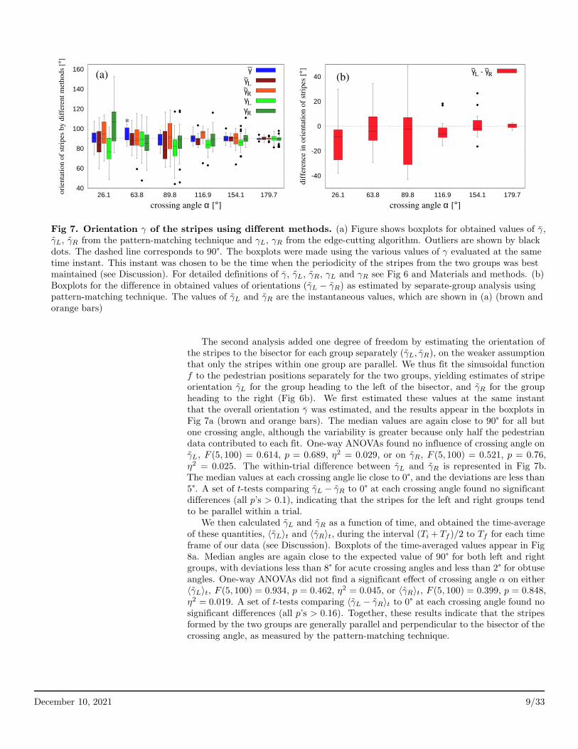
Fig 7. Orientation γ of the stripes using different methods. (a) Figure shows boxplots for obtained values of γ,γL, γR from the pattern-matching technique and γL, γR from the edge-cutting algorithm. Outliers are shown by blackdots. The dashed line corresponds to 90°. The boxplots were made using the various values of γ evaluated at the sametime instant. This instant was chosen to be the time when the periodicity of the stripes from the two groups was bestmaintained (see Discussion). For detailed definitions of γ, γL, γR, γL and γR see Fig 6 and Materials and methods. (b)Boxplots for the difference in obtained values of orientations (γL − γR) as estimated by separate-group analysis usingpattern-matching technique. The values of γL and γR are the instantaneous values, which are shown in (a) (brown andorange bars)

The second analysis added one degree of freedom by estimating the orientation ofthe stripes to the bisector for each group separately (γL, γR), on the weaker assumptionthat only the stripes within one group are parallel. We thus fit the sinusoidal functionf to the pedestrian positions separately for the two groups, yielding estimates of stripeorientation γL for the group heading to the left of the bisector, and γR for the groupheading to the right (Fig 6b). We first estimated these values at the same instantthat the overall orientation γ was estimated, and the results appear in the boxplots inFig 7a (brown and orange bars). The median values are again close to 90° for all butone crossing angle, although the variability is greater because only half the pedestriandata contributed to each fit. One-way ANOVAs found no influence of crossing angle onγL, F (5, 100) = 0.614, p = 0.689, η2 = 0.029, or on γR, F (5, 100) = 0.521, p = 0.76,η2 = 0.025. The within-trial difference between γL and γR is represented in Fig 7b.The median values at each crossing angle lie close to 0°, and the deviations are less than5°. A set of t-tests comparing γL − γR to 0° at each crossing angle found no significantdifferences (all p’s > 0.1), indicating that the stripes for the left and right groups tendto be parallel within a trial.

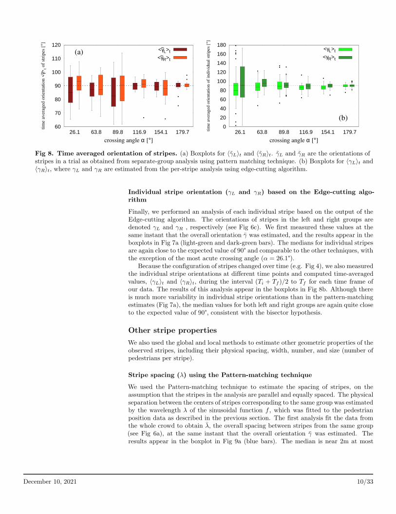
We then calculated γL and γR as a function of time, and obtained the time-averageof these quantities, 〈γL〉t and 〈γR〉t, during the interval (Ti + Tf )/2 to Tf for each timeframe of our data (see Discussion). Boxplots of the time-averaged values appear in Fig8a. Median angles are again close to the expected value of 90° for both left and rightgroups, with deviations less than 8° for acute crossing angles and less than 2° for obtuseangles. One-way ANOVAs did not find a significant effect of crossing angle α on either〈γL〉t, F (5, 100) = 0.934, p = 0.462, η2 = 0.045, or 〈γR〉t, F (5, 100) = 0.399, p = 0.848,η2 = 0.019. A set of t-tests comparing 〈γL − γR〉t to 0° at each crossing angle found nosignificant differences (all p’s > 0.16). Together, these results indicate that the stripesformed by the two groups are generally parallel and perpendicular to the bisector of thecrossing angle, as measured by the pattern-matching technique.

December 10, 2021 9/33

60

70

80

90

100

110

120

26.1 63.8 89.8 116.9 154.1 179.7

(a)

tim

e av

erag

ed o

rien

tati

on

<γ~ >

t of

stri

pes

[°]

crossing angle α [°]

<γ~L>t

<γ~R>t

0

20

40

60

80

100

120

140

160

180

26.1 63.8 89.8 116.9 154.1 179.7

(b)

tim

e av

erag

ed o

rien

tati

on

of

ind

ivid

ual

str

ipes

[°]

crossing angle α [°]

<γL>t

<γR>t

Fig 8. Time averaged orientation of stripes. (a) Boxplots for 〈γL〉t and 〈γR〉t. γL and γR are the orientations ofstripes in a trial as obtained from separate-group analysis using pattern matching technique. (b) Boxplots for 〈γL〉t and〈γR〉t, where γL and γR are estimated from the per-stripe analysis using edge-cutting algorithm.

Individual stripe orientation (γL and γR) based on the Edge-cutting algo-rithm

Finally, we performed an analysis of each individual stripe based on the output of theEdge-cutting algorithm. The orientations of stripes in the left and right groups aredenoted γL and γR , respectively (see Fig 6c). We first measured these values at thesame instant that the overall orientation γ was estimated, and the results appear in theboxplots in Fig 7a (light-green and dark-green bars). The medians for individual stripesare again close to the expected value of 90° and comparable to the other techniques, withthe exception of the most acute crossing angle (α = 26.1°).

Because the configuration of stripes changed over time (e.g. Fig 4), we also measuredthe individual stripe orientations at different time points and computed time-averagedvalues, 〈γL〉t and 〈γR〉t, during the interval (Ti + Tf )/2 to Tf for each time frame ofour data. The results of this analysis appear in the boxplots in Fig 8b. Although thereis much more variability in individual stripe orientations than in the pattern-matchingestimates (Fig 7a), the median values for both left and right groups are again quite closeto the expected value of 90°, consistent with the bisector hypothesis.

Other stripe properties

We also used the global and local methods to estimate other geometric properties of theobserved stripes, including their physical spacing, width, number, and size (number ofpedestrians per stripe).

Stripe spacing (λ) using the Pattern-matching technique

We used the Pattern-matching technique to estimate the spacing of stripes, on theassumption that the stripes in the analysis are parallel and equally spaced. The physicalseparation between the centers of stripes corresponding to the same group was estimatedby the wavelength λ of the sinusoidal function f , which was fitted to the pedestrianposition data as described in the previous section. The first analysis fit the data fromthe whole crowd to obtain λ, the overall spacing between stripes from the same group(see Fig 6a), at the same instant that the overall orientation γ was estimated. Theresults appear in the boxplot in Fig 9a (blue bars). The median is near 2m at most

December 10, 2021 10/33

crossing angles, but drops to 1.3m in the counterflow condition. A one-way ANOVAfound that λ depended significantly on crossing angle α, F (5, 100) = 3.426, p = 0.0067,η2 = 0.15. A trend analysis revealed significant linear through 5th-order trends (all p’s< 0.01), indicating that the relationship was irregular, not monotonic (see S3 Fig). Inthe second analysis, we fit each group independently to estimate the stripe spacing forthe left and right groups, λL, λR (see Fig 6b), at the same instant. These results alsoappear in Fig 9(a) (brown and orange bars), and exhibit a similar drop in stripe widthin the counterflow condition. One-way ANOVAs found a significant effect of crossingangle on λL, F (5, 100) = 3.817, p = 0.0033, η2 = 0.16, but not on λR, F (5, 100) = 1.781,p = 0.124, η2 = 0.082, likely due to the higher variability in the latter group. A trendanalysis found no significant trends for either λL or λR (all p’s > 0.08, see S3 Fig).

0

0.5

1

1.5

2

2.5

3

3.5

4

4.5

26.1 63.8 89.8 116.9 154.1 179.7

spat

ial

separ

atio

n b

etw

een

two s

trip

es f

rom

the

sam

e gro

up [

m]

(a)

_

crossing angle α [°]

λλ~

L

λ~

R 0

0.5

1

1.5

2

2.5

3

3.5

26.1 63.8 89.8 116.9 154.1 179.7

(b)

dif

fere

nce

in s

pat

ial

separ

atio

n [

m]

crossing angle α [°]

|λ_

- λ~

L|

|λ_

- λ~

R|

0

0.5

1

1.5

2

2.5

26.1 63.8 89.8 116.9 154.1 179.7

(c)

tim

e-av

erag

ed d

iffe

ren

ce i

n s

pat

ial

sep

arat

ion

[m

]

crossing angle α [°]

<|λ~L-λ~R|>t

Fig 9. Boxplots for λ as estimated from the pattern matching technique. λ is the spatial separation betweentwo alternate stripes from the same group. (a) The boxplots were made over all the trials for obtained values of λ, λLand λR at the instant when the periodicity of the two groups was best maintained. λ, λL and λR are defined inMaterials and methods. (b) Boxplots for the difference between obtained values of spatial separations from thewhole-crowd and separate-group analyses under the pattern matching procedure. (c) Time-averaged difference ofphysical separation 〈|λL − λR|〉t, where λL and λR are the physical separations between stripes in a trial as estimatedfrom the separate-group analysis using pattern matching technique.

To compare the overall spacing of the crowd with the separate spacing in eachgroup, we computed the absolute difference between them on each trial, |λ − λL| and|λ− λR|. The median differences (Fig 9b) are generally between 0.5m and 1m for acuteand orthogonal crossing angles, but less than 0.2m for obtuse crossing angles. One-way

December 10, 2021 11/33

ANOVAs confirmed that these differences significantly depended on crossing angle: for|λ− λL| , F (5, 100) = 3.648, p = 0.0045, η2 = 0.154; for |λ− λR|, F (5, 100) = 5.796, p <0.001, η2 = 0.224. Finally, we compared the stripe spacing in the left and right groupson each trial by computing the time-average of the difference 〈|∆λ|〉t = 〈|λL − λR|〉t,during the interval (Ti+Tf)/2 to Tf for each time frame of our data. The results suggestthat stripe spacing differed between groups by more than 0.6m at acute crossing angles,but by less than 0.4m at larger angles (Fig 9c). A one-way ANOVA on 〈|∆λ|〉t confirmeda significant dependence on crossing angle, F (5, 100) = 4.26, p = 0.0015, η2 = 0.175.

Stripe width, number, and size based on the Edge-cutting algo-

rithm

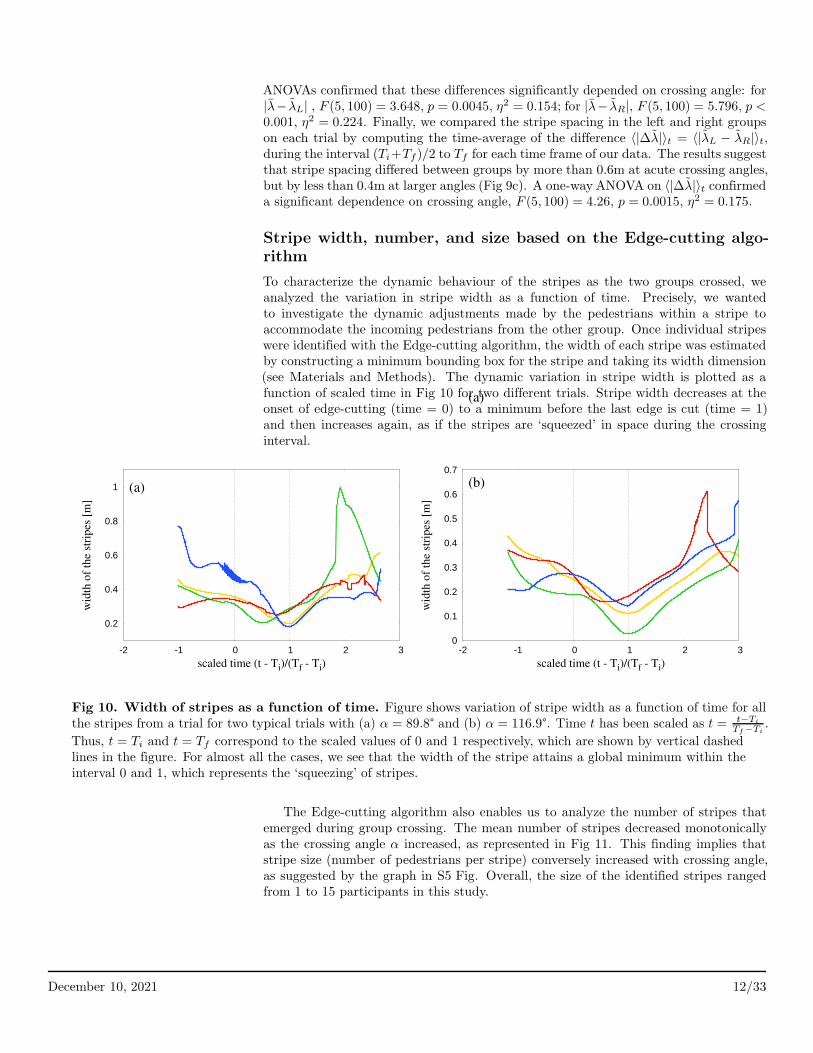
To characterize the dynamic behaviour of the stripes as the two groups crossed, weanalyzed the variation in stripe width as a function of time. Precisely, we wantedto investigate the dynamic adjustments made by the pedestrians within a stripe toaccommodate the incoming pedestrians from the other group. Once individual stripeswere identified with the Edge-cutting algorithm, the width of each stripe was estimatedby constructing a minimum bounding box for the stripe and taking its width dimension(see Materials and Methods). The dynamic variation in stripe width is plotted as afunction of scaled time in Fig 10 for two different trials. Stripe width decreases at theonset of edge-cutting (time = 0) to a minimum before the last edge is cut (time = 1)and then increases again, as if the stripes are ‘squeezed’ in space during the crossinginterval.

0.2

0.4

0.6

0.8

1

-2 -1 0 1 2 3

(a)

wid

th o

f th

e st

ripes

[m

]

scaled time (t - Ti)/(Tf - Ti)

0

0.1

0.2

0.3

0.4

0.5

0.6

0.7

-2 -1 0 1 2 3

(a)

(b)

wid

th o

f th

e st

ripes

[m

]

scaled time (t - Ti)/(Tf - Ti)

Fig 10. Width of stripes as a function of time. Figure shows variation of stripe width as a function of time for allthe stripes from a trial for two typical trials with (a) α = 89.8° and (b) α = 116.9°. Time t has been scaled as t = t−Ti

Tf−Ti.

Thus, t = Ti and t = Tf correspond to the scaled values of 0 and 1 respectively, which are shown by vertical dashedlines in the figure. For almost all the cases, we see that the width of the stripe attains a global minimum within theinterval 0 and 1, which represents the ‘squeezing’ of stripes.

The Edge-cutting algorithm also enables us to analyze the number of stripes thatemerged during group crossing. The mean number of stripes decreased monotonicallyas the crossing angle α increased, as represented in Fig 11. This finding implies thatstripe size (number of pedestrians per stripe) conversely increased with crossing angle,as suggested by the graph in S5 Fig. Overall, the size of the identified stripes rangedfrom 1 to 15 participants in this study.

December 10, 2021 12/33

4

5

6

7

26.1 63.8 89.8 116.9 154.1 179.7

(b)

mea

n n

um

ber

of

stri

pes

per

gro

up

α [°]

Fig 11. Mean number of stripes emerging from a group. Figure shows thevariation of this quantity with crossing angle α. The mean was estimated over all thetrials of our experiments. The number decreases with increasing α. The error-barsindicate the corresponding standard errors of mean.

Discussion

In this section we discuss the formation of striped patterns and their geometric prop-erties as observed and estimated from our experimental data. This is followed by anevaluation of the two computational methods we used to derive our findings.

Did we observe stripe formation?

Analyzing the formation of stripes was the main goal of this research. In our experi-ments, we found that stripe formation occurs even in small groups of pedestrians withfewer than 20 members, crossing in different directions without spatial constraints. Thisdemonstrates that continuous flows in constrained channels are not necessary for self-organized pattern formation, which can be attributed to local interactions. We shouldpoint out that, there could have been a number of outcomes. For example, the twogroups could have avoided without even penetrating each other, resulting in no for-mation of stripes. Large difference in velocities of the two groups could result in thisscenario; thus the velocity of the two groups plays a crucial role in this context. An-other possibility might be that crossing groups produced single isolated pedestrians, i.e.,all the virtual connections between the pedestrians from one group were destroyed bypedestrians from the other group. This situation would also result in absence of stripeformation. The two groups avoiding each other and the isolation of single pedestriansare the two extreme possibilities of outcomes from our experiments. In reality we sawthat the two groups indeed penetrate each other. The edge-cutting algorithm revealedthe groups of around 20 participants, divided into 4 to 7 subgroups, as shown in Fig11. This confirms that not all pedestrians from a group end up being isolated as aconsequence of crossing. The identification of the participants belonging to a stripe wasthen used to calculate the orientation and width of the stripe. Several examples of theedge-cutting process are shown in Fig 4 and 12.

December 10, 2021 13/33

-10

-5

0

5

10

-10 -5 0 5 10

(a)

α = 63.8°

(i)

Ti - 1

y [

m]

x [m]

-10

-5

0

5

10

-10 -5 0 5 10

(ii)

(Ti + Tf)/2

y [

m]

x [m]

-10

-5

0

5

10

-10 -5 0 5 10

(iii)

Tf + 1 y [

m]

x [m]

-10

-5

0

5

10

-10 -5 0 5 10

(iv)

(Ti + Tf)/2

y [

m]

x [m]

-10

-5

0

5

10

-10 -5 0 5 10

(v)

Ti - 1

y [

m]

x [m]

-10

-5

0

5

10

-10 -5 0 5 10

(b)

α = 154.1°

y [

m]

x [m]

-10

-5

0

5

10

-10 -5 0 5 10

y [

m]

x [m]

-10

-5

0

5

10

-10 -5 0 5 10

y [

m]

x [m]

-10

-5

0

5

10

-10 -5 0 5 10

y [

m]

x [m]

-10

-5

0

5

10

-10 -5 0 5 10

y [

m]

x [m]

Fig 12. Examples of the edge-cutting process. Edge-cutting process for two trials with (a) α = 63.8° and (b)α = 154.1°. The blue and red arrows denote the directions of motion for the two groups of pedestrians shown by blueand red dots respectively. The instances shown in this figure goes forward in time from (i) to (iii) and backward in timefrom (iii) to (v). In (i) the instance shown is Ti − 1, when all the edges within a group are intact. (ii) Shows thesituation when the edges have started to cut and stripes are gradually being formed at (Ti + Tf)/2. (iii) Shows thesituation at Tf + 1 when all probable edge-cuts have taken place and the stripes have completely been formed. (iv) and(v) shows the instances as in (ii) and (i) respectively but with the visualisation of all the stripes that are completelyformed only after Tf .

December 10, 2021 14/33

Do the stripe properties depend on crossing angle?

We were primarily interested in the effect of crossing angle on the orientation γ of thestripes with respect to the bisector of the crossing angle. Based on previous observationsand simulations, the expected value of γ = 90° should be invariant over different valuesof crossing angle α. The results obtained from our experimental data using severalmethods of measurement are shown in Fig 7a. The deviation of the median value of γremained less than 3° at all crossing angles, which is in good agreement with the bisectorhypothesis.

Spatial separation λ between two stripes from the same group was output from thepattern matching technique. We compared the values of λ estimated using whole-crowdand separate-group analysis in Fig 9a as a function of α.

Estimations of individual stripe properties based on the Edge-cutting algorithmrevealed that the mean number of stripes that emerges from a group decreases with α,as shown in Fig 11. This implies that the mean size of a stripe should show an increasewith α. In S5 Fig we have shown the plot of mean size of a stripe as a function of thecrossing angle α. The mean stripe size indeed increases with α. Thus the edge-cuttingalgorithm is very useful to establish the dependence of individual stripe properties onthe crossing angle.

Comparison of assumptions and results for the whole-crowd and

separate-group analyses using the pattern matching technique

To perform pattern matching using a two dimensional sinusoid we make two differentassumptions about the formation of stripes. In our analysis of finding γ and λ, weassumed that the orientation of the two groups are parallel to each other and thestripes formed are periodic and equispaced. However we kept in mind that in realitythis might not always be true. The orientation of the stripes for the two groups couldbe different and have different spacing. Thus, in a preliminary analysis we estimatedstripe orientation γ and their physical separation λ for the two groups separately asa function of time. In this approach we assumed that the stripes within one groupare parallel to each other and equispaced. The time window which was selected forthis analysis was from Ti to Tf . The two timescales Ti and Tf were estimated fromthe Edge-cutting algorithm, and they approximately denote the beginning and end ofinteraction, between the two groups.

γ and λ for each groups show some fluctuations near Ti i.e. when the stripes havejust started to form (see S4 Fig). The fluctuations reduce with time and the values ofγ and λ approach a more steady value near Tf i.e. when the stripes have been formed.Thus we calculate 〈γL〉t and 〈γR〉t, i.e., the time averages of γL and γR (shown in Fig8(a)) and the time-averaged difference 〈|∆λ|〉t = 〈|λL − λR|〉t (shown in Fig 9c) from(Ti + Tf )/2 to Tf i.e. when γ and λ remain approximately steady.

The differences of median values of 〈γL〉t and 〈γR〉t from the expected value of 90°are less than 2° for cases with an obtuse angle, and less than 8° for cases with an acutecrossing angle with no statistical effect of crossing angle. This approximately justifiesour earlier assumption about the orientation of stripes from two groups being parallelto each other. The time averaged difference in stripe spacing between the two groups〈|∆λ|〉t also shows low median values - less than 0.8 m for all the crossing angles. Thisalso justifies our assumption of parallel stripes from two groups when using the patternmatching technique.

We also make a comparative analysis of the differences in values of physical spacingof the stripes at the same time instant obtained by whole-crowd and separate-groupanalyses under the pattern matching technique. The results for |λ − λL| and |λ − λR|

December 10, 2021 15/33

are shown in Fig 9b. The median values of the differences are less than 0.2 m for obtusecrossing angles, but are higher for acute crossing angles.

There was a possibility of ‘chevron’ effect to create the differences in observed valuesof γL and γR. But due to the small size of our groups, the pedestrians might tend tomove faster while leaving the crossing region - resulting in the absence of chevron effect.The non-uniformity in the velocities of the agents both within the group and across thegroups could also lead to deformation of stripes. One explanation could be the durationof time when the two groups keep interacting with each other. For lower values ofα this duration is higher (see S6 Fig), which results in deformation in the symmetricstructure of the stripes. There could also be an effect of the size of the environmentwhere the experiments were performed. Because of limitation of space used for theexperiments, the two groups start interacting immediately after the commencement oftrials for lower crossing angles. So there is a possibility that the agents participatingfor trials with acute crossing angle (e.g. 30°) are still accelerating when reaching thecrossing region, which clearly is not the case for trials with higher crossing angles. Toinvestigate this further one needs to perform an analysis with larger number of peoplein a bigger environment and eventually, with a flow of people - not just two groupscrossing each other.

To analyse the statistical dependence of obtained results on the two methods underpattern matching technique we performed ANOVAs for each of the crossing anglesseparately. For γ, γL and γR ANOVAs reveal no dependence of these quantities on thetwo methods for each of the crossing angles. For each of the cases the p-value is greaterthan 0.145. For λ, λL and λR, the results were seen to be statistically independentof the two methods except for the case α = 89.8°, as could also be seen from Fig 9a.Except α = 89.8°, the p-values are greater than 0.266. The results of the ANOVAs areshown in supplementary material (S1 Table and S2 Table).

Comparing results between pattern matching technique and the

edge-cutting algorithm

Using the edge-cutting algorithm we have conducted a per-stripe analysis, where prop-erties of individual stripes were studied. This helps us in a minimal way to explorethe apparent asymmetry in the stripes from the two groups, which has been discussedearlier. The edge-cutting algorithm gives us the knowledge of stripes formed viz. thepedestrians belonging to a stripe. Using this output we compute the orientation andwidth of each of the stripes by implying rotating calipers algorithm (see Materials andMethods). The orientations γL and γR were computed as a time series. The timeaveraged orientation 〈γL〉t and 〈γR〉t were computed in the time interval (Ti + Tf )/2to Tf . The boxplots over all the stripes and all the trials are shown in Fig 8b. Thedifference of the median values of these average quantities from the expected orientation(90°) are less than 5° for obtuse crossing angles, but are a bit higher for acute crossingangles - a trend similar to previously discussed observations. The values of γL and γRcomputed at the same instant as when γ were computed, are shown in Fig 7a. In all thecases we observe that for obtuse crossing angles the stripe orientations obtained by theedge-cutting algorithm are not very different from that obtained by the pattern match-ing technique. However, for the acute crossing angles the differences are a bit higher- possible for reasons which have already been discussed. The width of the stripes asestimated from the per stripe analysis are not actually comparable to the physical sepa-ration of the stripes as computed by pattern matching technique. The stripes consistedof different numbers of people - this causes an irregularity while we attempt to computetheir individual orientation. As a consequence, it would be inappropriate to comparethese values with the outputs of the pattern matching technique, where the symmetry

December 10, 2021 16/33

and periodicity of the stripes were assumed. However, we see that the median valuesof the average quantities 〈γL〉t and 〈γR〉t are not very far (approximately within 10° forall crossing angles) from the expected value (90°), which was computed assuming thesymmetry and regularity of the stripes. This shows consistency across the methods thatwe have used to study stripe properties.

Why did we use two different methods?

The two computational methods that we present in this paper have never been usedbefore to study striped patterns in crossing flows, to the best of our knowledge. We usedthe two methods, viz. the edge-cutting algorithm and pattern matching technique, tostudy the formation and geometric properties of the stripes. The edge-cutting algorithmtakes into consideration the entire trajectories of the pedestrians, whereas for the patternmatching technique the instantaneous positions of the pedestrians are sufficient. Onlythe edge-cutting algorithm can identify a stripe and the pedestrians belonging to it. Thisyields a better definition of individual stripes and allows refined analysis of individualstripes, and is thus a spatially local method. Besides, this algorithm provides thefull dynamics of individual stripes, and is the most appropriate to study dynamicaleffects such as the ’squeezing effect’ of Fig 10 that we shall discuss shortly after. Whenthe stripes are very small (less than 3 participants) or are not sufficiently elongated(see Materials and Methods), their geometric properties are not well defined and weexcluded them from our per stripe analysis. On the other hand, the pattern matchingtechnique uses a two-dimensional parametric sinusoid and is thus a spatially globalmethod. This idea was inspired by Gabor functions, which have been used to modelthe spatial frequency response of the mammalian visual system [69]. We assume theexistence of a periodic pattern of parallel stripes and then use this method to look forit; these assumptions have been borne out by the similarity of orientation and spacingwhen measured in the whole crowd and separately for the two groups. For our small-scale data the pattern matching technique is essential to study the orientation of thestripes.

How efficient is the pattern matching technique?

The pattern matching technique that we have used to find the orientation γ of stripesand their spacial separation λ, was based on maximising C. C is obtained by fittinga two-dimensional sinusoid f on the coordinates of the pedestrians (see Materials andMethods). Therefore C could be treated like a scoring function which indicates thequality of fitting. For the case when we assume that stripes from the two groups areparallel to each other and alternately equispaced (to find γ, λ), the maximising functionis denoted by C and when we fitted the two groups separately (to find γ, λ), this functionwas denoted by C.

Importance of C and λ

For best fittings one would get C = Cmax = 2 and C = Cmax = 1, and for the worstcase (disordered input points) the sinusoidal function would not fit - it would eitherover-fit or under-fit the data points. Over-fitting or under-fitting could be identifiedby the obtained value of spatial separation λ between the stripes. The obtained valueof λ was therefore very crucial to justify the pattern matching technique. From edge-cutting algorithm one could have an approximate idea of the spatial separation betweentwo stripes for a trial (see Materials and Methods). λ would be very low or very highcompared to this approximate value in case of over-fitting and under-fitting respectively.The quality of the pattern matching technique is therefore estimated both in terms of C

December 10, 2021 17/33

0.2

0.3

0.4

0.5

0.6

0.7

0.8

0.9

1

26.1 63.8 89.8 116.9 154.1 179.7

the

fun

ctio

n w

hic

h w

as m

axim

ised

in p

atte

rn m

atch

ing

tec

hn

iqu

e (a)

_ _

~ ~~ ~

crossing angle α [°]

C/Cmax

CL/Cmax

CR/Cmax 0.2

0.3

0.4

0.5

0.6

0.7

0.8

0.9

1

26.1 63.8 89.8 116.9 154.1 179.7

~

~

(b)

crossing angle α [°]

<CL>t

<CR>t

Fig 13. Boxplots for the maximising function of pattern matching technique. (a) Boxplots for C/Cmax andC/Cmax, where C is the maximising function of pattern matching procedure of whole-crowd analysis and C is the samewith separate group-analysis. Cmax and Cmax are the maximum possible values of the maximising functions in thesetwo cases, which are 2 and 1 respectively. (b) Boxplots for the time-averaged values of CL and CR.

and by the optimised value of λ. Fig 5 (right) shows the variation of C as a function ofλ for two typical trials. In Fig 13 we have shown boxplots for the values of C for each ofthe crossing angles, as obtained by whole-crowd and separate-group analysis under thepattern matching technique. Higher values of C indeed signify a better fitting. FromFig 13 we see that the median values of both C and C increase with α. One-wayANOVAs on C found a significant effect of crossing angle on C, F (5, 100) = 17.53,p < 0.001, η2 = 0.467, on CL, F (5, 100) = 7.955, p < 0.001, η2 = 0.285, and on CR,F (5, 100) = 3.665, p = 0.0043, η2 = 0.155.

Estimating residual error of the fitting

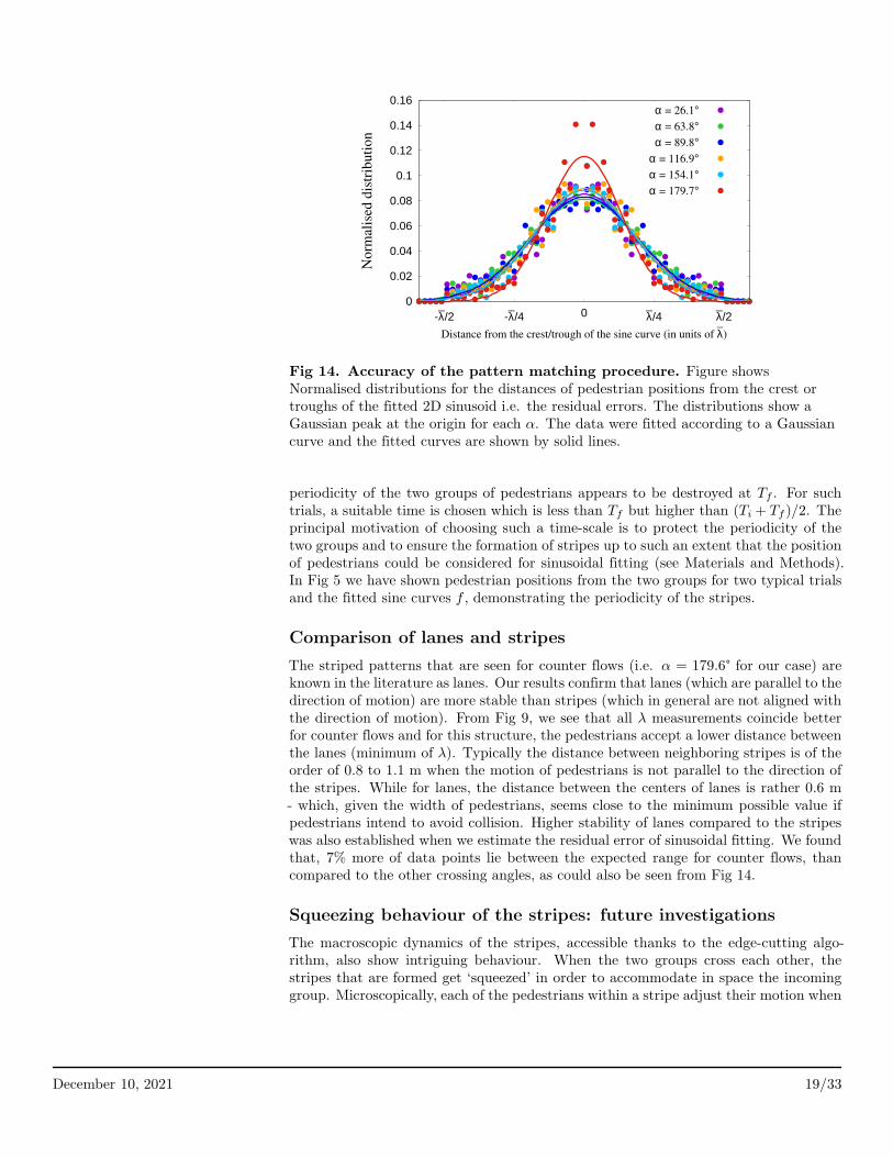
To study the accuracy of the pattern matching procedure to find γ and λ, we calculatethe residual errors. Ideally one would expect all the data points to lie within the distance−λ/4 to λ/4, where λ is the wavelength of the fitted sine curved f . We calculated theresidual error of pattern matching technique as the distance of the data points fromthe crest or trough of the fitted sine function f . The results are shown in Fig 14. Thenormalised distribution of this distance shows a Gaussian peak at the origin. We fit thedata for each of the cases using the functional form of Gaussian distribution. From thefittings, we estimate the standard deviations. For α = 179.9° the standard deviation ofthe fitted curve was 0.134λ and for the remaining crossing angles this value is 0.184λon average. From the data of residual error, we found that for α = 179.6°, 92.4% ofthe data points are accumulated between the distances −λ/4 and −λ/4, and for theremaining crossing angles, on an average 85.3% of the data is within this range. Thissurely establishes the efficiency of pattern fitting to a great extent. Besides, this alsounderlines a difference in stability between lanes and stripes (discussed later).

Periodicity of the two groups

The periodic arrangement of stripes that are seen to form in our experiments havebeen a point of concern for the pattern matching technique. An important aspect ofour pattern fitting procedure is to choose the instant of time for which the positionof pedestrians are considered and fitted. For higher values of α this instant is usuallywhen all the edges have been cut and all possible clusters have been formed, which isTf - an output from the Edge-cutting algorithm. However, for lower values of α the

December 10, 2021 18/33

0

0.02

0.04

0.06

0.08

0.1

0.12

0.14

0.16

-λ_/2 -λ

_/4 0 λ

_/4 λ

_/2

No

rmal

ised

dis

trib

uti

on

Distance from the crest/trough of the sine curve (in units of λ_

)

α = 26.1°α = 63.8°α = 89.8°

α = 116.9°α = 154.1°α = 179.7°

Fig 14. Accuracy of the pattern matching procedure. Figure showsNormalised distributions for the distances of pedestrian positions from the crest ortroughs of the fitted 2D sinusoid i.e. the residual errors. The distributions show aGaussian peak at the origin for each α. The data were fitted according to a Gaussiancurve and the fitted curves are shown by solid lines.

periodicity of the two groups of pedestrians appears to be destroyed at Tf . For suchtrials, a suitable time is chosen which is less than Tf but higher than (Ti + Tf )/2. Theprincipal motivation of choosing such a time-scale is to protect the periodicity of thetwo groups and to ensure the formation of stripes up to such an extent that the positionof pedestrians could be considered for sinusoidal fitting (see Materials and Methods).In Fig 5 we have shown pedestrian positions from the two groups for two typical trialsand the fitted sine curves f , demonstrating the periodicity of the stripes.

Comparison of lanes and stripes

The striped patterns that are seen for counter flows (i.e. α = 179.6° for our case) areknown in the literature as lanes. Our results confirm that lanes (which are parallel to thedirection of motion) are more stable than stripes (which in general are not aligned withthe direction of motion). From Fig 9, we see that all λ measurements coincide betterfor counter flows and for this structure, the pedestrians accept a lower distance betweenthe lanes (minimum of λ). Typically the distance between neighboring stripes is of theorder of 0.8 to 1.1 m when the motion of pedestrians is not parallel to the direction ofthe stripes. While for lanes, the distance between the centers of lanes is rather 0.6 m- which, given the width of pedestrians, seems close to the minimum possible value ifpedestrians intend to avoid collision. Higher stability of lanes compared to the stripeswas also established when we estimate the residual error of sinusoidal fitting. We foundthat, 7% more of data points lie between the expected range for counter flows, thancompared to the other crossing angles, as could also be seen from Fig 14.

Squeezing behaviour of the stripes: future investigations

The macroscopic dynamics of the stripes, accessible thanks to the edge-cutting algo-rithm, also show intriguing behaviour. When the two groups cross each other, thestripes that are formed get ‘squeezed’ in order to accommodate in space the incominggroup. Microscopically, each of the pedestrians within a stripe adjust their motion when

December 10, 2021 19/33

they encounter a pedestrian from the opposite group. In Fig 10 we have shown widthof all the stripes from two typical trials as a function of a scaled time for each crossingangle α. The time is scaled in such a way that the scaled value of 0 and 1 correspondto Ti and Tf of the trial. It is observed from Fig 10 that between the interval 0 and1 i.e. the beginning and end of interactions, the width of the stripes decreases, attainsa global minimum and then increases again. This indicates some interesting underly-ing microscopic behaviour of the agents, which results in the squeezing behaviour as amacroscopic property of the stripes. In our subsequent research we would be interestedto determine the underlying mechanism responsible for this behaviour. It would also beappealing to find out whether a following behaviour is present among the pedestriansleading to the formation of stripes, which we plan to work in our next research.

Conclusion

We conducted experimental trials for crossing flows of pedestrians without any spatialconstraints of motion. In spite of having small number of participants we observedthe formation of emerging striped patterns for each value of the crossing angle. Edge-cutting algorithm was implemented to detect the formation of stripes. Striped patternsfor counter flows i.e lanes are seen to be more stable than those for other crossingangles. We have used a pattern matching technique and the edge-cutting algorithmto study a few properties of the stripes formed and compare them with each otherand with hypothesized effects. The observed values for the orientation of stripes fromedge-cutting algorithm are in good agreement with the expected result which justifiesthat our assumption about the regularity and symmetry of the striped patterns arereasonable enough. The maximised values of C as obtained by us signify the regularityof the striped patterns from the two groups. While performing numerical simulations tomodel the scenario of crossing flows, the quantity C would act as a parameter to evaluatethe effectiveness of the simulation technique in reproducing the observed behaviour. Wenot only confirmed that stripe orientation is predicted by the bisector hypothesis at allcrossing angles, but we also discovered several unexpected effects. First we showed thatthe average number of stripes within a group decreases with the crossing angle alpha.Second, we found that the spacing, number, and size of stripes depended significantly oncrossing angle. Third, we observed a squeezing effect visible in the time evolution of thestripes. The macroscopic dynamics of the stripes motivates us to study the microscopicbehaviour of the individual pedestrians as our next investigation.

Materials and methods

Experimental details

The participants of the experiments were divided into two groups (with similar spatialdensities). They were instructed to move along a direction which was announced beforethe commencement of each trial, such that the two groups cross each other at a particularangle. For 7 different expected values of crossing angles, viz. [0°, 30°, 60°, 90°, 120°,150° and 180°], we performed approximately 17 trials at each angle, a total of 116 trials(See Table 1). During each trial the head trajectory of each pedestrian was recorded asa time series. Each trial lasted about 15-25 seconds. The experiment was performedin a rectangular hall (20m x 30m) with a tracking area of 15m x 20m. The positionsof the pedestrians were recorded at 120 Hz using VICON - an infrared camera system.The pedestrians were equipped with head-mounted reflective markers detectable bythe VICON motion capture system. The center of the tracking was considered as theorigin of a two-dimensional Cartesian coordinate system, which was used as a reference

December 10, 2021 20/33

I

I

F

F

L

L

R

R

crossingangle

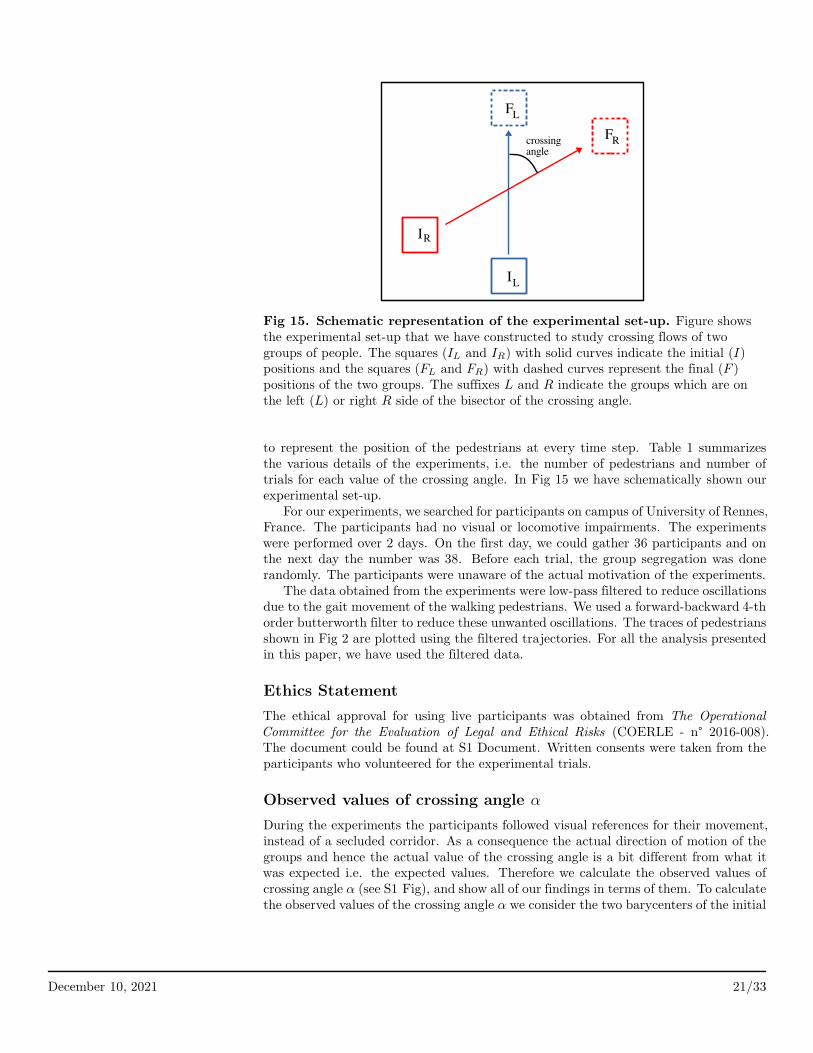
Fig 15. Schematic representation of the experimental set-up. Figure showsthe experimental set-up that we have constructed to study crossing flows of twogroups of people. The squares (IL and IR) with solid curves indicate the initial (I)positions and the squares (FL and FR) with dashed curves represent the final (F )positions of the two groups. The suffixes L and R indicate the groups which are onthe left (L) or right R side of the bisector of the crossing angle.

to represent the position of the pedestrians at every time step. Table 1 summarizesthe various details of the experiments, i.e. the number of pedestrians and number oftrials for each value of the crossing angle. In Fig 15 we have schematically shown ourexperimental set-up.

For our experiments, we searched for participants on campus of University of Rennes,France. The participants had no visual or locomotive impairments. The experimentswere performed over 2 days. On the first day, we could gather 36 participants and onthe next day the number was 38. Before each trial, the group segregation was donerandomly. The participants were unaware of the actual motivation of the experiments.

The data obtained from the experiments were low-pass filtered to reduce oscillationsdue to the gait movement of the walking pedestrians. We used a forward-backward 4-thorder butterworth filter to reduce these unwanted oscillations. The traces of pedestriansshown in Fig 2 are plotted using the filtered trajectories. For all the analysis presentedin this paper, we have used the filtered data.

Ethics Statement

The ethical approval for using live participants was obtained from The Operational

Committee for the Evaluation of Legal and Ethical Risks (COERLE - n° 2016-008).The document could be found at S1 Document. Written consents were taken from theparticipants who volunteered for the experimental trials.

Observed values of crossing angle α

During the experiments the participants followed visual references for their movement,instead of a secluded corridor. As a consequence the actual direction of motion of thegroups and hence the actual value of the crossing angle is a bit different from what itwas expected i.e. the expected values. Therefore we calculate the observed values ofcrossing angle α (see S1 Fig), and show all of our findings in terms of them. To calculatethe observed values of the crossing angle α we consider the two barycenters of the initial

December 10, 2021 21/33

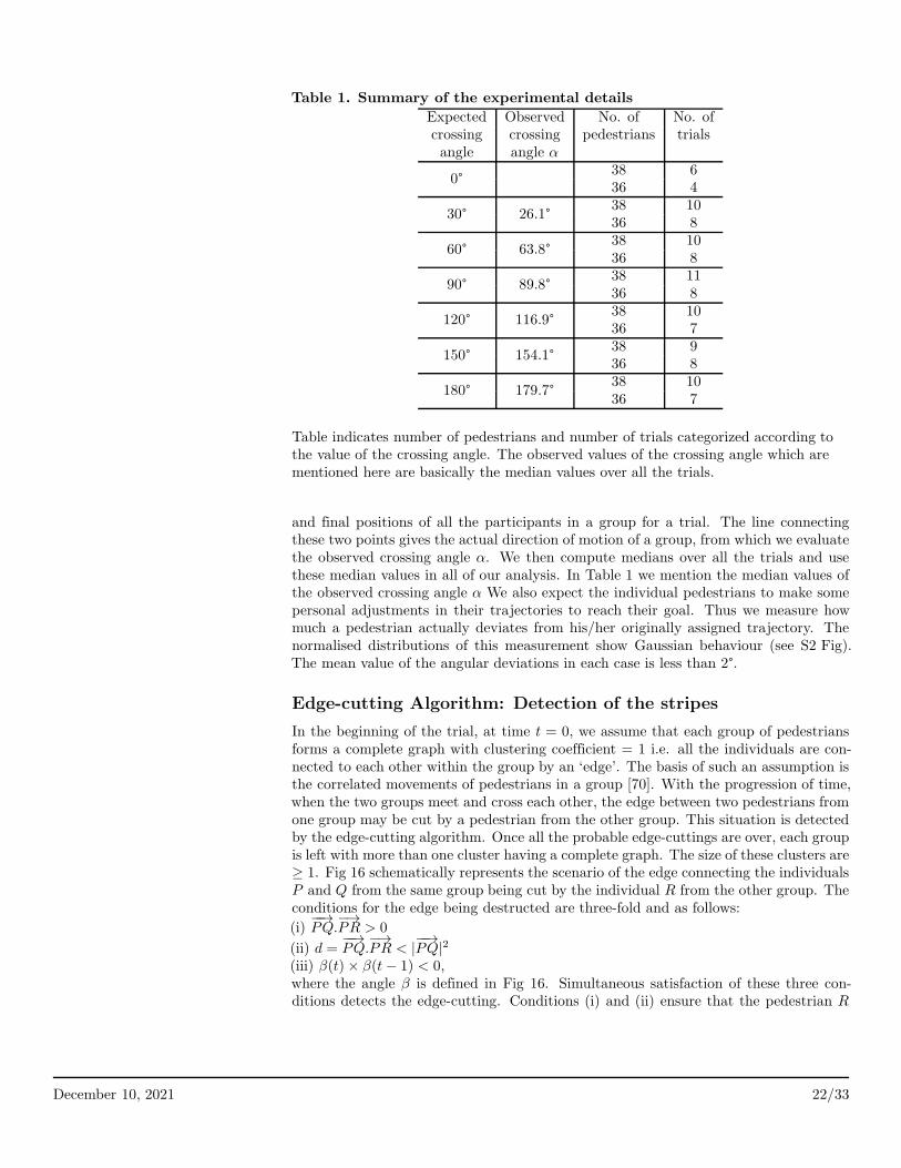
Table 1. Summary of the experimental details

Expected Observed No. of No. ofcrossing crossing pedestrians trialsangle angle α

0°38 636 4

30° 26.1°38 1036 8

60° 63.8°38 1036 8

90° 89.8°38 1136 8

120° 116.9°38 1036 7

150° 154.1°38 936 8

180° 179.7°38 1036 7

Table indicates number of pedestrians and number of trials categorized according tothe value of the crossing angle. The observed values of the crossing angle which arementioned here are basically the median values over all the trials.

and final positions of all the participants in a group for a trial. The line connectingthese two points gives the actual direction of motion of a group, from which we evaluatethe observed crossing angle α. We then compute medians over all the trials and usethese median values in all of our analysis. In Table 1 we mention the median values ofthe observed crossing angle α We also expect the individual pedestrians to make somepersonal adjustments in their trajectories to reach their goal. Thus we measure howmuch a pedestrian actually deviates from his/her originally assigned trajectory. Thenormalised distributions of this measurement show Gaussian behaviour (see S2 Fig).The mean value of the angular deviations in each case is less than 2°.

Edge-cutting Algorithm: Detection of the stripes

In the beginning of the trial, at time t = 0, we assume that each group of pedestriansforms a complete graph with clustering coefficient = 1 i.e. all the individuals are con-nected to each other within the group by an ‘edge’. The basis of such an assumption isthe correlated movements of pedestrians in a group [70]. With the progression of time,when the two groups meet and cross each other, the edge between two pedestrians fromone group may be cut by a pedestrian from the other group. This situation is detectedby the edge-cutting algorithm. Once all the probable edge-cuttings are over, each groupis left with more than one cluster having a complete graph. The size of these clusters are≥ 1. Fig 16 schematically represents the scenario of the edge connecting the individualsP and Q from the same group being cut by the individual R from the other group. Theconditions for the edge being destructed are three-fold and as follows:

(i)−−→PQ.

−→PR > 0

(ii) d =−−→PQ.

−→PR < |

−−→PQ|2

(iii) β(t)× β(t− 1) < 0,where the angle β is defined in Fig 16. Simultaneous satisfaction of these three con-ditions detects the edge-cutting. Conditions (i) and (ii) ensure that the pedestrian R

December 10, 2021 22/33

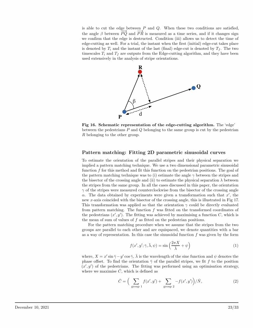
is able to cut the edge between P and Q. When these two conditions are satisfied,

the angle β between−−→PQ and

−→PR is measured as a time series, and if it changes sign

we confirm that the edge is destructed. Condition (iii) allows us to detect the time ofedge-cutting as well. For a trial, the instant when the first (initial) edge-cut takes placeis denoted by Ti and the instant of the last (final) edge-cut is denoted by Tf . The twotimescales Ti and Tf are outputs from the Edge-cutting algorithm, and they have beenused extensively in the analysis of stripe orientations.

P

Q

R

d

β

Fig 16. Schematic representation of the edge-cutting algorithm. The ‘edge’between the pedestrians P and Q belonging to the same group is cut by the pedestrianR belonging to the other group.

Pattern matching: Fitting 2D parametric sinusoidal curves

To estimate the orientation of the parallel stripes and their physical separation weimplied a pattern matching technique. We use a two dimensional parametric sinusoidalfunction f for this method and fit this function on the pedestrian positions. The goal ofthe pattern matching technique was to (i) estimate the angle γ between the stripes andthe bisector of the crossing angle and (ii) to estimate the physical separation λ betweenthe stripes from the same group. In all the cases discussed in this paper, the orientationγ of the stripes were measured counterclockwise from the bisector of the crossing angleα. The data obtained by experiments were given a transformation such that x′, thenew x-axis coincided with the bisector of the crossing angle, this is illustrated in Fig 17.This transformation was applied so that the orientation γ could be directly evaluatedfrom pattern matching. The function f was fitted on the transformed coordinates ofthe pedestrians (x′, y′). The fitting was achieved by maximising a function C, which isthe mean of sum of values of f as fitted on the pedestrian positions.

For the pattern matching procedure when we assume that the stripes from the twogroups are parallel to each other and are equispaced, we denote quantities with a baras a way of representation. In this case the sinusoidal function f was given by the form

f(x′, y′; γ, λ, ψ) = sin(2πX

λ+ ψ

)

(1)

where, X = x′ sin γ−y′ cos γ, λ is the wavelength of the sine function and ψ denotes thephase offset. To find the orientation γ of the parallel stripes, we fit f to the position(x′, y′) of the pedestrians. The fitting was performed using an optimisation strategy,where we maximise C, which is defined as

C =(

∑

group 1

f(x′, y′) +∑

group 2

−f(x′, y′))

/N , (2)

December 10, 2021 23/33

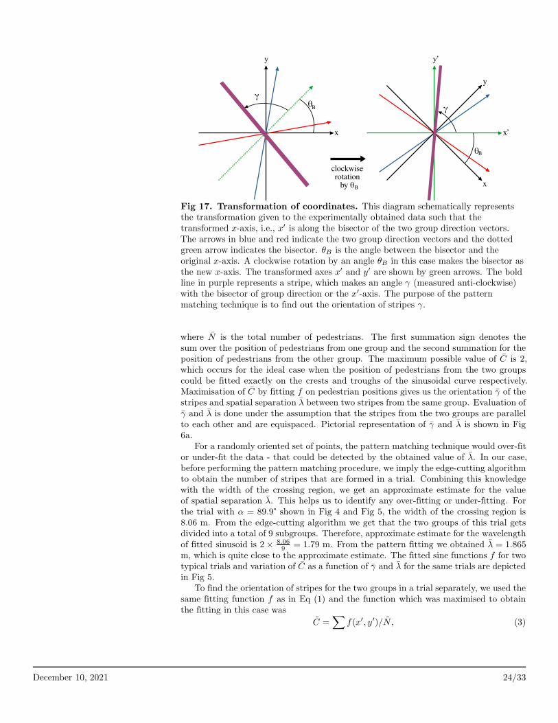
γ

γθ

θ

B

B

x x’

x

y y’

y

clockwiserotationby θB

Fig 17. Transformation of coordinates. This diagram schematically representsthe transformation given to the experimentally obtained data such that thetransformed x-axis, i.e., x′ is along the bisector of the two group direction vectors.The arrows in blue and red indicate the two group direction vectors and the dottedgreen arrow indicates the bisector. θB is the angle between the bisector and theoriginal x-axis. A clockwise rotation by an angle θB in this case makes the bisector asthe new x-axis. The transformed axes x′ and y′ are shown by green arrows. The boldline in purple represents a stripe, which makes an angle γ (measured anti-clockwise)with the bisector of group direction or the x′-axis. The purpose of the patternmatching technique is to find out the orientation of stripes γ.

where N is the total number of pedestrians. The first summation sign denotes thesum over the position of pedestrians from one group and the second summation for theposition of pedestrians from the other group. The maximum possible value of C is 2,which occurs for the ideal case when the position of pedestrians from the two groupscould be fitted exactly on the crests and troughs of the sinusoidal curve respectively.Maximisation of C by fitting f on pedestrian positions gives us the orientation γ of thestripes and spatial separation λ between two stripes from the same group. Evaluation ofγ and λ is done under the assumption that the stripes from the two groups are parallelto each other and are equispaced. Pictorial representation of γ and λ is shown in Fig6a.

For a randomly oriented set of points, the pattern matching technique would over-fitor under-fit the data - that could be detected by the obtained value of λ. In our case,before performing the pattern matching procedure, we imply the edge-cutting algorithmto obtain the number of stripes that are formed in a trial. Combining this knowledgewith the width of the crossing region, we get an approximate estimate for the valueof spatial separation λ. This helps us to identify any over-fitting or under-fitting. Forthe trial with α = 89.9° shown in Fig 4 and Fig 5, the width of the crossing region is8.06 m. From the edge-cutting algorithm we get that the two groups of this trial getsdivided into a total of 9 subgroups. Therefore, approximate estimate for the wavelengthof fitted sinusoid is 2× 8.06

9= 1.79 m. From the pattern fitting we obtained λ = 1.865

m, which is quite close to the approximate estimate. The fitted sine functions f for twotypical trials and variation of C as a function of γ and λ for the same trials are depictedin Fig 5.

To find the orientation of stripes for the two groups in a trial separately, we used thesame fitting function f as in Eq (1) and the function which was maximised to obtainthe fitting in this case was

C =∑

f(x′, y′)/N, (3)

December 10, 2021 24/33

where the summation was performed over the position of pedestrians from one group ata time. N is the number of pedestrians in the group. The maximum possible value of Cis 1, which in this case occurs for the ideal situation when the pedestrian positions fromthe group under consideration fall exactly on the crests of the sine curve representedby f . This analysis was performed as a time sequence between (Ti + Tf)/2 and Tf .

Maximisation of C by fitting f on the pedestrian positions gives us the orientation γ ofthe stripes and the spatial separation λ between the stripes from the same group. Thiscomputation was done under the assumption that the stripes from the same group areparallel to each other and have equal spacing between them.

While fitting the parallel stripes from the two groups separately we differentiatethem by using the notations γL and γR. γL denotes the orientation of the stripes whosegroup direction vector lies to the left (L) of the direction of bisector and similarly, γRfor the one whose group direction vector lies to the right (R) of the direction of bisector.Similarly, we use the notations λL and λR to denote the spatial separation between thestripes from the same group, according to the orientation of its group direction vectorwith respect to the bisector. Pictorial demonstration of γL, γR, λL and λR are shownin Fig 6b. Following the same convention, the functions that were maximised to obtain(γL, λL) and (γR, λR) were denoted as CL and CR respectively.

For the segregation of the groups according to whether they lie to the left or right ofthe bisector of the crossing angle, it is therefore important to determine the direction ofthe bisector. This direction is estimated using the two group direction vectors. But forthe case of crossing angle 180°, determining the direction of the bisector is not possible.However we realise that the experimentally observed value of the crossing angle α isnever exactly equal to 180°. Thus estimating the direction of bisector for these cases isalso pretty straight-forward.

Finding individual stripe width and orientation

From the Edge-cutting algorithm we could successfully identify the stripes that areformed. In our attempt to find the individual stripe orientations at each instant weconstruct the minimum bounding box of the stripes using Rotating Calipers algorithm[71, 72]. The orientation of the stripe was calculated along the length of the box. Thewidth of the rectangular box gives an estimate of the width of each of the stripes. Theaspect ratio of the minimum bounding box for a stripe, calculated as the ratio of itswidth to length, gives an idea of the suitability of that stripe to be considered for theestimation of orientation. The value of aspect ratio closer to 1 denotes a uniformlyshaped stripe. Whereas, lower value of aspect ratio indicates a sufficiently elongatedstripe suitable for finding the orientation. In Figure 18, we show two typical stripeswith their respective minimum bounding boxes calculated using the Rotating Calipersalgorithm. We applied a cut-off on aspect ratios of the stripes and considered only thosestripes which had an aspect ratio less than 0.5. The time window which was selected forthis calculation was from (Ti + Tf )/2 to Tf . The orientation of individual stripes werealso estimated as the angle between the stripes and the bisector of the group directionvectors, as depicted in Fig 6c. The angle is measured counterclockwise from the bisector.We use the notations γL and γR to differentiate the orientation of stripes whose groupdirection vector lie to the left and right of the bisector respectively.

Supporting information

S1 Table. Results of ANOVAs for γ, γL and γR for each α. Table summarizesthe results of the ANOVA tests that were performed for each α with γ, γL and γR to

December 10, 2021 25/33

��� ���

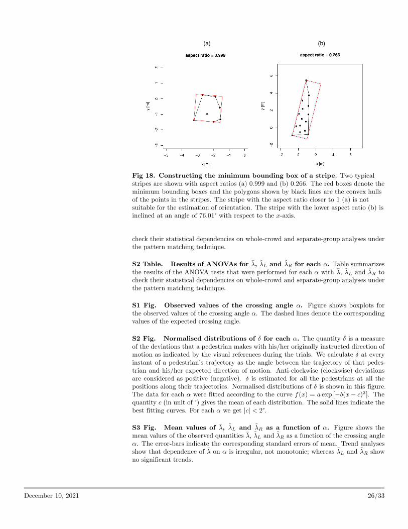
Fig 18. Constructing the minimum bounding box of a stripe. Two typicalstripes are shown with aspect ratios (a) 0.999 and (b) 0.266. The red boxes denote theminimum bounding boxes and the polygons shown by black lines are the convex hullsof the points in the stripes. The stripe with the aspect ratio closer to 1 (a) is notsuitable for the estimation of orientation. The stripe with the lower aspect ratio (b) isinclined at an angle of 76.01° with respect to the x-axis.

check their statistical dependencies on whole-crowd and separate-group analyses underthe pattern matching technique.

S2 Table. Results of ANOVAs for λ, λL and λR for each α. Table summarizesthe results of the ANOVA tests that were performed for each α with λ, λL and λR tocheck their statistical dependencies on whole-crowd and separate-group analyses underthe pattern matching technique.

S1 Fig. Observed values of the crossing angle α. Figure shows boxplots forthe observed values of the crossing angle α. The dashed lines denote the correspondingvalues of the expected crossing angle.

S2 Fig. Normalised distributions of δ for each α. The quantity δ is a measureof the deviations that a pedestrian makes with his/her originally instructed direction ofmotion as indicated by the visual references during the trials. We calculate δ at everyinstant of a pedestrian’s trajectory as the angle between the trajectory of that pedes-trian and his/her expected direction of motion. Anti-clockwise (clockwise) deviationsare considered as positive (negative). δ is estimated for all the pedestrians at all thepositions along their trajectories. Normalised distributions of δ is shown in this figure.The data for each α were fitted according to the curve f(x) = a exp [−b(x− c)2]. Thequantity c (in unit of °) gives the mean of each distribution. The solid lines indicate thebest fitting curves. For each α we get |c| < 2°.

S3 Fig. Mean values of λ, λL and λR as a function of α. Figure shows themean values of the observed quantities λ, λL and λR as a function of the crossing angleα. The error-bars indicate the corresponding standard errors of mean. Trend analysesshow that dependence of λ on α is irregular, not monotonic; whereas λL and λR showno significant trends.

December 10, 2021 26/33

S4 Fig. Time sequence of γ and λ estimated separately for the two groups ina trial. The plots are shown for two typical trials with (a) α = 63.8° and (b) α = 154.1°.The time window for which the data is shown is between the respective values of Ti andTf for both the trials. Ti and Tf are evaluated the Edge-cutting algorithm. For γ plotsin the left panel, the dashed lines indicate 90°, the expected value of stripe orientationand for λ plots in the right panel, the dashed lines indicate the value of λ as estimatedfrom the pattern matching technique by considering the two groups together.

S5 Fig. Mean size of stripes as a function of α. The size of a stripes is defined asthe number of pedestrians belonging to that stripe. The mean size of a stripe increaseswith the increase of crossing angle. The error-bars indicate the corresponding standarderrors of mean.

S6 Fig. Mean crossing time as a function of α. Crossing time for each trial isdefined as Tf − Ti, where Ti and Tf are estimated from the edge-cutting algorithm. Tiand Tf denotes the time when the first and last edge-cut takes place for the trial. Themean crossing time over all the trials decreases with the increase of crossing angle. Theerror-bars indicate the corresponding standard errors of mean.

S1 Video. Video of the experimental trial which is shown in Fig 1

S2 Video. Edge-cutting process for a trial with α = 89.8° which is shown inFig 4. In this video we show the edge-cutting process for a typical trial with α = 89.8°,the one which has been shown in Fig 4. The time frames are shown in scales of t−Ti

Tf−Ti.

S3 Video. Edge-cutting process for a trial with α = 116.9° which is shownin Fig 4. Same as the previous item with with α = 116.9°.

S1 Document. Ethical approval statement.

Acknowledgments

The authors gratefully thank A. Sorel, A. Cretual, G. Dachner, and T. Wirth for theirhelp in conducting the experimental trials. A. Marin is also acknowledged for helpingin data processing from the camera system.

Funding Information

Pratik Mullick thanks financial support from Bretagne S.A.D. as allocated in the projecttitled ATTRACT. Sylvain Fontaine acknowledges support for his internship by the“Investissements d’Avenir” of LabEx PALM (ANR-10-LABX-0039-PALM), in the frameof the PERCEFOULE project.

Author Contributions

Conceptualization:Pratik Mullick, William H. Warren, Cecile Appert-Rolland, Anne-Helene Olivier, JulienPettre

Data Curation:Sylvain Fontaine, Anne-Helene Olivier, Julien Pettre

December 10, 2021 27/33

Formal Analysis:Pratik Mullick, William H. Warren, Cecile Appert-Rolland

Funding Acquisition:Julien Pettre, Cecile Appert-Rolland

Investigation:Pratik Mullick, William H. Warren, Cecile Appert-Rolland, Julien Pettre

Methodology:Pratik Mullick, Sylvain Fontaine, William H. Warren, Cecile Appert-Rolland, JulienPettre

Project Administration:Julien Pettre

Resources:Julien Pettre

Software:Pratik Mullick, Sylvain Fontaine, Anne-Helene Olivier

Supervision:William H. Warren, Cecile Appert-Rolland, Julien Pettre

Validation:Pratik Mullick, Sylvain Fontaine, William H. Warren, Cecile Appert-Rolland, JulienPettre

Visualization:Pratik Mullick

Writing – Original Draft Preparation:Pratik Mullick

Writing – Review & Editing:Pratik Mullick, William H. Warren, Cecile Appert-Rolland, Julien Pettre

References

1. John A, Schadschneider A, Chowdhury D, Nishinari K. Collective effects in traf-fic on bi-directional ant trails, 2004 J Theor Biol 2004 231(2): 279-285 doi:10.1016/j.jtbi.2004.06.022.

2. Gautrais J, Ginelli F, Fournier R, Blanco S, Soria M, et al. Deciphering Inter-actions in Moving Animal Groups. PLoS Comput Biol 2012 8(9): e1002678. doi:10.1371/journal.pcbi.1002678

3. Moussaıd M, Guillot EG, Moreau M, Fehrenbach J, Chabiron O, et al. TrafficInstabilities in Self-Organized Pedestrian Crowds. PLoS Comput Biol 2012 8(3):e1002442 doi: 10.1371/journal.pcbi.1002442

4. Perna A, Granovskiy B, Garnier S, Nicolis SC, Labedan M, et al. IndividualRules for Trail Pattern Formation in Argentine Ants (Linepithema humile). PLOSComput Biol 2012 8(7): e1002592. doi: 10.1371/journal.pcbi.1002592

5. Fujii K, Kawasaki T, Inaba Y, Kawahara Y. Prediction and classificationin equation-free collective motion dynamics. PLOS Comput Biol 2018 14(11):e1006545. doi: 10.1371/journal.pcbi.1006545

6. Stormbom D, Dussutour A. Self-organized traffic via priority rules in leaf-cutting ants. PLoS Comput Biol 2018 14(10): e1006523. doi: 10.1371/jour-nal.pcbi.1006523

December 10, 2021 28/33

7. Rio KW, Dachner GC, Warren WH. Local interactions underlying collec-tive motion in human crowds. 2018 Proc R Soc B, 285: 20180611. doi:10.1098/rspb.2018.0611

8. Thompson P A, Marchant E W. A computer model for the evacuation oflarge building populations. Fir Saf J 1995 24(2): 131-148. doi: 10.1016/0379-7112(95)00019-P

9. Helbing D, Farkas I, Vicsek T. Simulating dynamical features of escape panic.Nature 2000 407: 487-490. doi: 10.1038/35035023

10. Pedestrian and Evacuation Dynamics, edited by Schreckenberg M and SharmaSD. Berlin: Springer; 2002.

11. He G-Q, Yang Y, Chen Z-H, Gu C-H. A review of behavior mechanisms andcrowd evacuation animation in emergency exercises. J Zhejiang Univ - Sci 2013C 14: 477–485 doi: 10.1631/jzus.CIDE1301

12. Bohannon J. Directing the herd: Crowds and the science of evacuation. Science2005 310(5746): 219-221. doi: 10.1126/science.310.5746.219

13. Hoogendoorn SP, Hauser M, Rodrigues N. Applying Microscopic Pedestrian FlowSimulation to Railway Station Design Evaluation in Lisbon, Portugal. Transp ResRec J Transp Res Board 2004 1878(1): 83-94. doi:10.3141/1878-11

14. Helbing D, Johansson A, Al-Abideen H Z. Dynamics of crowd disasters: Anempirical study. Phys Rev E 2007 75: 046109. doi: 10.1103/PhysRevE.75.046109

15. Johansson A, Helbing D, Al-Abideen H Z, Al-bosta S. From crowd dynamics tocrowd safety: A video-based analysis. Adv Complex Syst 2008 11(4): 497–527.doi: 10.1142/S0219525908001854

16. Bain N, Bartolo D. Dynamic response and hydrodynamics of polarised crowds.Science 2019 363(6422): 46-49. doi: 10.1126/science.aat9891

17. Batty M, DeSyllas J, Duxbury E, The Discrete Dynamics of Small-Scale SpatialEvents: Agent-Based Models of Mobility in Carnivals and Street Parades. Int JGeograph Inf Sci 2003 17: 673-697. doi: 10.1080/1365881031000135474

18. Lee R S, Hughes R L, Exploring Trampling and Crushing in a Crowd, J TranspEng 2005 131(8): 575-582 doi: 10.1061/(ASCE)0733-947X(2005)131:8(575)

19. Seyfried A, Steffen B, Klingsch W, Boltes M. The fundamental diagram ofpedestrian movement revisited. J Stat Mech 2005 P10002. doi: 10.1088/1742-5468/2005/10/P10002

20. Chattaraj U, Seyfried A, and Chakroborty P. Comparison of pedestrian funda-mental diagram across cultures. Adv Complex Syst 2009 12(3): 393-405. doi:10.1142/S0219525909002209

21. Seyfried A, Boltes M, Kahler J, Klingsch W, Portz A et al. Enhanced Empiri-cal Data for the Fundamental Diagram and the Flow Through Bottlenecks. In:Klingsch W, Rogsch C, Schadschneider A, Schreckenberg M (editors) Pedestrianand Evacuation Dynamics 2008; pp 145-156. Springer, Berlin, Heidelberg. doi:10.1007/978-3-642-04504-2 11

22. Jezbera D, Kordek D, Krız1 J, Seba P and Sroll P. Walkers on the circle. J StatMech 2010 L01001. doi: 10.1088/1742-5468/2010/01/L01001

December 10, 2021 29/33

23. Yanagisawa D, Tomoeda A, Nishinari K. Improvement of pedestrian flow by slowrhythm. Phys Rev E 2012 85: 016111 doi: 10.1103/PhysRevE.85.016111

24. Jelic A, Appert-Rolland C, Lemercier S, Pettre J. Properties of pedestri-ans walking in line: Fundamental diagrams. Phys Rev E 2012 85: 036111.doi: 10.1103/PhysRevE.85.036111 and Properties of pedestrians walking inline. II. Stepping behavior. Phys Rev E 2012 86: 046111. doi: 10.1103/Phys-RevE.86.046111

25. Olivier A-H, Marin A, Cretual A, Pettre J. Minimal predicted distance: A com-mon metric for collision avoidance during pairwise interactions between walkers.Gait Posture 2012 36(3): 399-404. doi: 10.1016/j.gaitpost.2012.03.021

26. Olivier A-H, Marin A, Cretual A, Pettre J. Collision avoidance between twowalkers: Role-dependent strategies. Gait Posture 2013 38(4): 751-756. doi:10.1016/j.gaitpost.2013.03.017

27. Meerhoff LA, Pettre J, Lynch SD, Cretual A, Olivier A-H. Collision AvoidanceWith Multiple Walkers: Sequential or Simultaneous Interactions? Front Psychol2018 9:2354 doi: 10.3389/fpsyg.2018.02354

28. Hoogendoorn S, Daamen W. Pedestrian behavior at bottlenecks. Transp Sci 200539(2): 147–159. doi: 10.1287/trsc.1040.0102

29. Kretz T, Grunebohm S, and Schreckenberg M. Experimental study of pedes-trian flow through a bottleneck. J Stat Mech 2006 P10014. doi: 10.1088/1742-5468/2006/10/P10014

30. Seyfried A, Passon O, Steffen B, Boltes M, Rupprecht T, Klingsch W. New in-sights into pedestrian flow through bottlenecks. Transp Sci 2009 43(3): 395-406.doi: 10.1287/trsc.1090.0263

31. Faure S, Maury B. Crowd motion from the granular standpoint. Math ModelsMethods Appl Sci 2015 25: 463–493. doi: 10.1142/S0218202515400035

32. Garcimartın A, Parisi D, Pastor J, Martn-Gomez C, Zuriguel I. Flow of pedes-trians through narrow doors with different competitiveness. J Stat Mech 2016043402 (2016). doi: 10.1088/1742-5468/2016/04/043402

33. Nicolas, A., Bouzat, S., Kuperman, M. N. Pedestrian flows through a narrowdoorway: Effect of individual behaviours on the global flow and microscopicdynamics. Transport Res B-Meth 2017 99: 30–43. doi: 10.1016/j.trb.2017.01.008

34. Zhang J, Klingsch W, Schadschneider A and Seyfried A. Transitions in pedestrianfundamental diagrams of straight corridors and T-junctions. J Stat Mech 2011 6P06004 doi: 10.1088/1742-5468/2011/06/P06004

35. Zhang J, KlingschW, Schadschneider A, Seyfried A. Experimental Study of Pedes-trian Flow Through a T-Junction. In: Kozlov V, Buslaev A, Bugaev A, YashinaM, Schadschneider A, Schreckenberg M. (editors) Traffic and Granular Flow 2011.Springer, Berlin, Heidelberg. doi: 10.1007/978-3-642-39669-4 23

36. Cao S, Seyfried A, Zhang J, Holl S and Song W. Fundamental diagrams formultidirectional pedestrian flows. J Stat Mech 2017 033404. doi: 10.1088/1742-5468/aa620d

December 10, 2021 30/33

37. Appert-Rolland C, Pettre J, Olivier A-H, Warren W, Duigou-Majumdar A etal. Experimental Study of Collective Pedestrian Dynamics. Collective Dynamics2020 5: 1-8. ISSN: 2366-8539. doi: 10.17815/CD.2020.109

38. Nicolas A, Kuperman M, Ibanez S, Bouzat S, Appert-Rolland C. Mechanicalresponse of dense pedestrian crowds to the crossing of intruders. Sci Rep 2019 9:105. doi: 10.1038/s41598-018-36711-7

39. Adrian J, Boltes M, Holl S, Sieben A, Seyfried A. Crowding and Queuing in En-trance Scenarios: Influence of Corridor Width in Front of Bottlenecks. CollectiveDynamics 2020 5: 189-196. doi: 10.17815/CD.2020.50

40. Hoogendoorn S, Daamen W. Self-Organization in Pedestrian Flow. In: Hoogen-doorn SP, Luding S, Bovy PHL, Schreckenberg M, Wolf DE (editors) Traffic andGranular Flow 2003. Springer, Berlin, Heidelberg. doi: 10.1007/3-540-28091-X 36

41. Helbing D, Buzna L, Johansson A and Werner T. Self-organised pedestrian crowddynamics: Experiments, simulations and design solutions. Transp Sci 2005 39(1):1-24. doi: 10.1287/trsc.1040.0108

42. Kretz T, Grunebohm A, Kaufman M, Mazur F and Schreckenberg M. Experi-mental study of pedestrian counterflow in a corridor. J Stat Mech 2006 P10001.doi: 10.1088/1742-5468/2006/10/P10001

43. Zhang J, Klingsch W, Schadschneider A and Seyfried A. Ordering in bidirectionalpedestrian flows and its influence on the fundamental diagram. J Stat Mech 2012P02002. doi: 10.1088/1742-5468/2012/02/P02002

44. Feliciani C and Nishinari K. Empirical analysis of the lane formation process inbidirectional pedestrian flow. Phys Rev E 2016 94: 032304. doi: 10.1103/Phys-RevE.94.032304

45. Helbing D and Molnar P. Social force model for pedestrian dynamics. Phys RevE 1995 51: 4282. doi : 10.1103/PhysRevE.51.4282

46. Fukui M and Ishibashi Y. Self-organized phase transitions in cellular au-tomaton models for pedestrians. J Phys Soc Jpn 1999 68: 2861-2863. doi:10.1143/JPSJ.68.2861

47. Muramatsu M, Irie T and Nagatani T. Jamming transition in pedestrian counterflow. Phys A Stat Mech 1999 267(3): 487-498. doi: 10.1016/S0378-4371(99)00018-7

48. Helbing D. Traffic and related self-driven many-particle systems Rev Mod Phys2001 73: 1067. doi: 10.1103/RevModPhys.73.1067

49. Burstedde C, Klauck K, Schadschneider A Zittarz J. Simulation of pedestriandynamics using a 2-dimensional cellular automaton. Phys A Stat Mech 2001 295:507-525. doi: 10.1016/S0378-4371(01)00141-8

50. Blue VJ, Adler JL, Cellular automata microsimulation for modeling bi-directional pedestrian walkways. Transp Res B-Meth 2001 35(3): 293-312. url:https://ideas.repec.org/a/eee/transb/v35y2001i3p293-312.html

51. Tajima Y, Takimoto K, Nagatani T. Pattern formation and jamming transi-tion in pedestrian counter flow. Phys A Stat Mech 2002 313(3): 709-723. doi:10.1016/S0378-4371(02)00965-2

December 10, 2021 31/33

52. Dzubiella J, Lowen H. Pattern formation in driven colloidal mixtures: Tilteddriving forces and re-entrant crystal freezing. J Phys Condens Matter 2002 14:9383-9395. doi: 10.1088/0953-8984/14/40/324

53. Hoogendoorn S, Bovy PHL. Simulation of pedestrian flows by optimal con-trol and differential games. Optim Control Appl Meth 2003 24: 153-172. doi:10.1002/oca.727

54. Isobe M, Adachi T, Nagatani T. Experiment and simulation of pedestrian counterflow. Phys A Stat Mech 2004 336(3): 638-650. doi: 10.1016/j.physa.2004.01.043

55. Nagai R, Fukamachi M, Nagatani T. Experiment and simulation for counter-flow of people going on all fours. Phys A Stat Mech 2005 358(2): 516-528. doi:10.1016/j.physa.2005.04.024

56. Cristn J, Mendez, Campos D. General scaling in bidirectional flows of self-avoiding agents. Sci Rep 9, 18488. doi: 10.1038/s41598-019-54977-3

57. Khelfa B, Korbmacher R, Schadschneider A, Tordeux A. Heterogeneity-inducedlane and band formation in self-driven particle systems. arXiv:2110.05874[preprint]. 2021. Available from https://arxiv.org/abs/2110.05874.

58. Naka Y. Mechanism of cross passenger flow - Study on Complicated PassengerFlow in Railway Station (Part I) (in Japanese). Trans Arch Inst Jpn 1977 258:93-102

59. Ondrej J, Pettre J, Olivier A H, Donikian S. A Synthetic-Vision Based Steer-ing Approach for Crowd Simulation. ACM Trans Graphics 2010 29(4): 123. doi:10.1145/1778765.1778860

60. Yamamoto K, Okada M. Continuum Model of Crossing Pedestrian Flows andSwarm Control Based on Temporal/Spatial Frequency. In: 2011 IEEE Inter-national Conference on Robotics and Automation (ICRA). pp. 3352-3357. doi:10.1109/ICRA.2011.5980444

61. Cividini J, Appert-Rolland C, Hilhorst HJ. Diagonal patterns and chevron ef-fect in intersecting traffic flows. EPL 2013 102(2): 20002. doi: 10.1209/0295-5075/102/20002

62. Cividini J, Appert-Rolland C. Wake-mediated interaction between driven parti-cles crossing a perpendicular flow. J Stat Mech 2013 P07015. doi: 10.1088/1742-5468/2013/07/P07015

63. Cividini J, Hilhorst HJ and Appert-Rolland C. Crossing pedestrian traffic flows,the diagonal stripe pattern and the chevron effect. J Phys A Math Theor 201346: 345002. doi: 10.1088/1751-8113/46/34/345002

64. Cividini J, Hilhorst HJ. Stripe formation instability in crossing traffic flows. JPhys A Math Theor 2014 47: 445002. doi: 10.1088/1751-8113/47/44/445002

65. Wong S, ASCE M, Leung WL, Chan SH, Lam WHK et al. Bidirectional Pedes-trian Stream Model with Oblique Intersecting Angle. J Transp Eng 2010 136(3):234-242. doi: 10.1061/(ASCE)TE.1943-5436.0000086

66. Helbing D. Verkehrsdynamic [Traffic Dynamics]. Berlin: Springer-Verlag BerlinHeidelberg; 1997 doi: 10.1007/978-3-642-59063-4

December 10, 2021 32/33

67. Helbing D, Molnar P. Self-organisation phenomena in pedestrian crowds. In: F.Schweitzer (editor). Self-organisation of Complex Structures: From Individual toCollective Dynamics. London: Gordon and Breach; 1997 pp. 569-577.

68. Helbing D, Vicsek T. Optimal self-organisation. New J Phys 1999 1: 13. doi:10.1088/1367-2630/1/1/313

69. Marcelja S. Mathematical description of the responses of simple cortical cells. JOpt Soc Am 1980 70(11): 1297–1300. doi: 10.1364/JOSA.70.001297

70. Henderson LF. The Statistics of Crowd Fluids. Nature 1971 229: 381-383. doi:10.1038/229381a0

71. Shamos MI. Computational geometry. Ph.D. Thesis, YaleUniversity, New Haven, Connecticut, 1978. Available fromhttp://euro.ecom.cmu.edu/people/faculty/mshamos/1978ShamosThesis.pdf

72. Toussaint GT. Solving Geometric Problems with the Rotat-ing Calipers. Proc MELECON 1983, Athens. Available fromhttps://citeseerx.ist.psu.edu/viewdoc/summary?doi=10.1.1.155.5671

December 10, 2021 33/33