000 Momentum ENG rev2 20160322 error삭제phylab.yonsei.ac.kr/exp_ref/104_Momentum_ENG.pdf · Momentum and Impulse Ver.20160322 Lab Office (Int’l Campus) Room 301, Building 301

General Physics Lab (International Campus) Department of PHYSICS YONSEI University

Lab Manual

Momentum and ImpulseVer.20160322

Lab Office (Int’l Campus)

Room 301, Building 301 (Libertas Hall B), Yonsei University 85 Songdogwahak-ro, Yeonsu-gu, Incheon 21983, KOREA (☏ +82 32 749 3430) Page 1 / 17

[For International Campus Lab ONLY]

Momentum and Impulse

Investigate the relationship between impulse and momentum.

Many situations such as collision or explosion involve little

known forces exerted on bodies for a short time. Thus, they

cannot be analyzed by directly applying Newton’s second law,

∑ .

Two new concepts, momentum and impulse, and a new

conservation law, conservation of momentum, enable us to

analyze these situations.

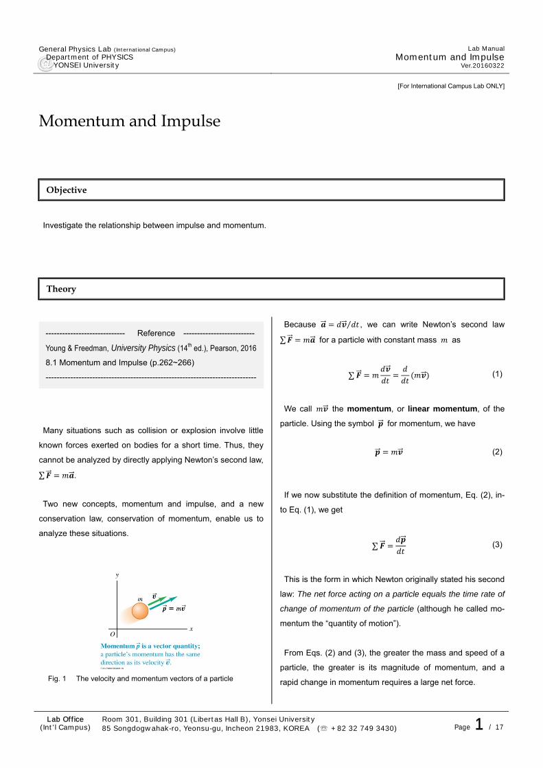
Fig. 1 The velocity and momentum vectors of a particle

Because ⁄ , we can write Newton’s second law

∑ for a particle with constant mass as

∑ (1)

We call the momentum, or linear momentum, of the

particle. Using the symbol for momentum, we have

(2)

If we now substitute the definition of momentum, Eq. (2), in-

to Eq. (1), we get

∑ (3)

This is the form in which Newton originally stated his second

law: The net force acting on a particle equals the time rate of

change of momentum of the particle (although he called mo-

mentum the “quantity of motion”).

From Eqs. (2) and (3), the greater the mass and speed of a

particle, the greater is its magnitude of momentum, and a

rapid change in momentum requires a large net force.

Objective

Theory

----------------------------- Reference --------------------------

Young & Freedman, University Physics (14th ed.), Pearson, 2016

8.1 Momentum and Impulse (p.262~266)

-----------------------------------------------------------------------------


Lab Manual




If a constant net force ∑ acts on a particle during a time

interval Δ from to , the impulse of the net force, de-

noted by , is defined to be the product of the net force and

the time interval:

∑ ∑ Δ (4)

If ∑ is constant, then ⁄ is also constant as in Eq. (3).

In this case, ⁄ is equal to the total change in momen-

tum during the time interval , divided by the

interval:

∑ (5)

∑ (6)

From Eqs. (4) and (6), we end up with a result called the

impulse-momentum theorem:

(7)

Eq. (7) shows that the change in momentum of a particle

during a time interval equals the impulse of the net force that

acts on the particle during that interval.

The impulse-momentum theorem also holds when forces

are not constant. To see this, we integrate both sides of Eq.

(3) over time between and :

∑ (8)

The integral on the left is defined to be the impulse during

this interval:

∑ (9)

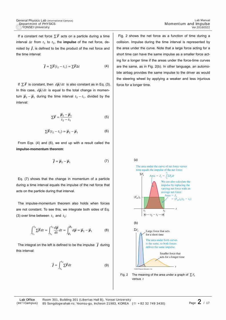
Fig. 2 shows the net force as a function of time during a

collision. Impulse during the time interval is represented by

the area under the curve. Note that a large force acting for a

short time can have the same impulse as a smaller force act-

ing for a longer time if the areas under the force-time curves

are the same, as in Fig. 2(b). In other language, an automo-

bile airbag provides the same impulse to the driver as would

the steering wheel by applying a weaker and less injurious

force for a longer time.

Fig. 2 The meaning of the area under a graph of ∑ versus


Lab Manual




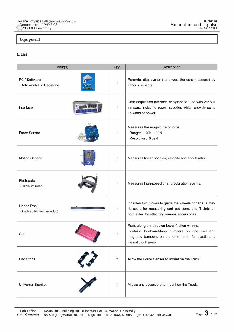
1. List

Item(s) Qty. Description

PC / Software

Data Analysis: Capstone

1 Records, displays and analyzes the data measured by

various sensors.

Interface

1

Data acquisition interface designed for use with various

sensors, including power supplies which provide up to

15 watts of power.

Force Sensor

1

Measures the magnitude of force.

Range: 50N~50N

Resolution: 0.03N

Motion Sensor

1 Measures linear position, velocity and acceleration.

Photogate

(Cable included)

1 Measures high-speed or short-duration events.

Linear Track

(2 adjustable feet included) 1

Includes two groves to guide the wheels of carts, a met-

ric scale for measuring cart positions, and T-slots on

both sides for attaching various accessories.

Cart

1

Runs along the track on lower-friction wheels.

Contains hook-and-loop bumpers on one end and

magnetic bumpers on the other end, for elastic and

inelastic collisions

End Stops

2 Allow the Force Sensor to mount on the Track.

Universal Bracket

1 Allows any accessory to mount on the Track.

Equipment


Lab Manual




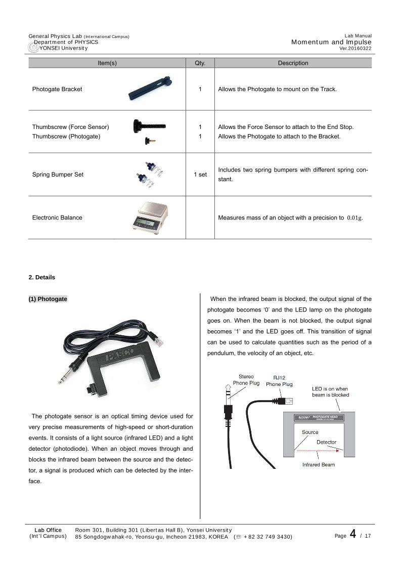
Item(s) Qty. Description

Photogate Bracket

1 Allows the Photogate to mount on the Track.

Thumbscrew (Force Sensor)

Thumbscrew (Photogate)

1

1

Allows the Force Sensor to attach to the End Stop.

Allows the Photogate to attach to the Bracket.

Spring Bumper Set

1 set Includes two spring bumpers with different spring con-

stant.

Electronic Balance

Measures mass of an object with a precision to 0.01g.

2. Details

(1) Photogate

The photogate sensor is an optical timing device used for

very precise measurements of high-speed or short-duration

events. It consists of a light source (infrared LED) and a light

detector (photodiode). When an object moves through and

blocks the infrared beam between the source and the detec-

tor, a signal is produced which can be detected by the inter-

face.

When the infrared beam is blocked, the output signal of the

photogate becomes ‘0’ and the LED lamp on the photogate

goes on. When the beam is not blocked, the output signal

becomes ‘1’ and the LED goes off. This transition of signal

can be used to calculate quantities such as the period of a

pendulum, the velocity of an object, etc.


Lab Manual




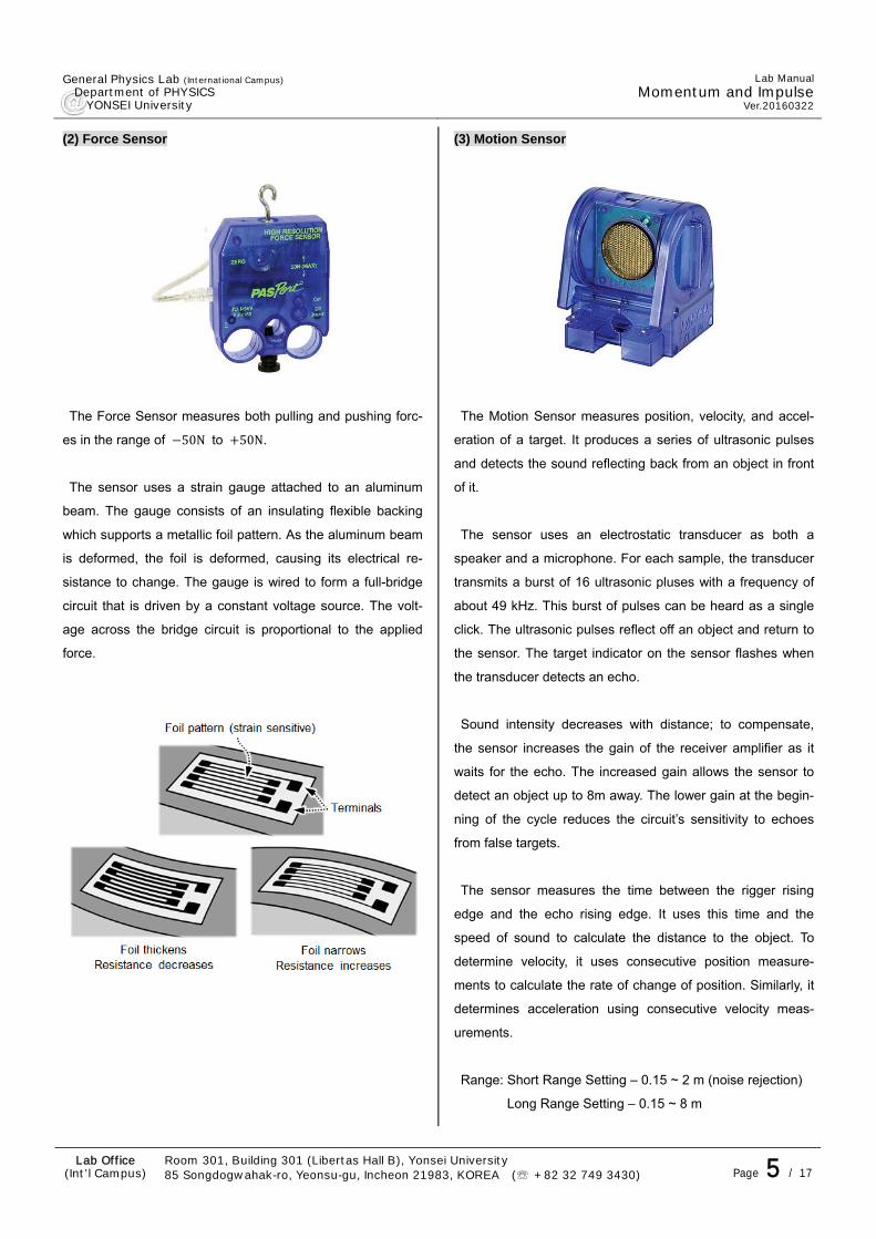
(2) Force Sensor

The Force Sensor measures both pulling and pushing forc-

es in the range of 50N to 50N.

The sensor uses a strain gauge attached to an aluminum

beam. The gauge consists of an insulating flexible backing

which supports a metallic foil pattern. As the aluminum beam

is deformed, the foil is deformed, causing its electrical re-

sistance to change. The gauge is wired to form a full-bridge

circuit that is driven by a constant voltage source. The volt-

age across the bridge circuit is proportional to the applied

force.

(3) Motion Sensor

The Motion Sensor measures position, velocity, and accel-

eration of a target. It produces a series of ultrasonic pulses

and detects the sound reflecting back from an object in front

of it.

The sensor uses an electrostatic transducer as both a

speaker and a microphone. For each sample, the transducer

transmits a burst of 16 ultrasonic pluses with a frequency of

about 49 kHz. This burst of pulses can be heard as a single

click. The ultrasonic pulses reflect off an object and return to

the sensor. The target indicator on the sensor flashes when

the transducer detects an echo.

Sound intensity decreases with distance; to compensate,

the sensor increases the gain of the receiver amplifier as it

waits for the echo. The increased gain allows the sensor to

detect an object up to 8m away. The lower gain at the begin-

ning of the cycle reduces the circuit’s sensitivity to echoes

from false targets.

The sensor measures the time between the rigger rising

edge and the echo rising edge. It uses this time and the

speed of sound to calculate the distance to the object. To

determine velocity, it uses consecutive position measure-

ments to calculate the rate of change of position. Similarly, it

determines acceleration using consecutive velocity meas-

urements.

Range: Short Range Setting – 0.15 ~ 2 m (noise rejection)

Long Range Setting – 0.15 ~ 8 m


Lab Manual




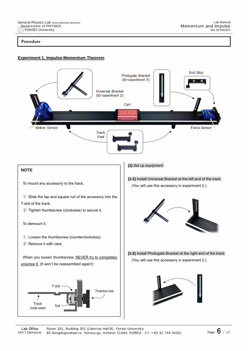
Experiment 1. Impulse-Momentum Theorem

(1) Set up equipment.

(1-1) Install Universal Bracket at the left end of the track.

(You will use this accessory in experiment 2.)

(1-2) Install Photogate Bracket at the right end of the track.

(You will use this accessory in experiment 2.)

Procedure

NOTE

To mount any accessory to the track,

① Slide the tap and square nut of the accessory into the

T-slot of the track.

② Tighten thumbscrew (clockwise) to secure it.

To demount it,

① Loosen the thumbscrew (counterclockwise).

② Remove it with care.

When you loosen thumbscrew, NEVER try to completely

unscrew it. (It won’t be reassembled again!)


Lab Manual




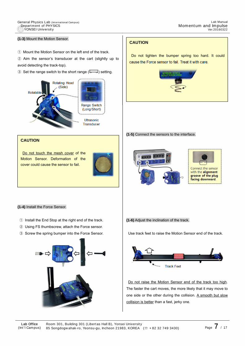
(1-3) Mount the Motion Sensor.

① Mount the Motion Sensor on the left end of the track.

② Aim the sensor’s transducer at the cart (slightly up to

avoid detecting the track-top).

③ Set the range switch to the short range ( ) setting.

(1-4) Install the Force Sensor.

① Install the End Stop at the right end of the track.

② Using FS thumbscrew, attach the Force sensor.

③ Screw the spring bumper into the Force Sensor.

(1-5) Connect the sensors to the interface.

(1-6) Adjust the inclination of the track.

Use track feet to raise the Motion Sensor end of the track.

Do not raise the Motion Sensor end of the track too high.

The faster the cart moves, the more likely that it may move to

one side or the other during the collision. A smooth but slow

collision is better than a fast, jerky one.

CAUTION

Do not touch the mesh cover of the

Motion Sensor. Deformation of the

cover could cause the sensor to fail.

CAUTION

Do not tighten the bumper spring too hard. It could

cause the Force sensor to fail. Treat it with care.


Lab Manual




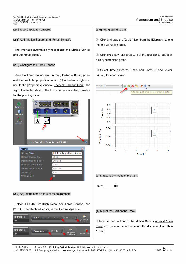
(2) Set up Capstone software.

(2-1) Add [Motion Sensor] and [Force Sensor].

The interface automatically recognizes the Motion Sensor

and the Force Sensor.

(2-2) Configure the Force Sensor.

Click the Force Sensor icon in the [Hardware Setup] panel

and then click the properties button (☼) in the lower right cor-

ner. In the [Properties] window, Uncheck [Change Sign]. The

sign of collected data of the Force sensor is initially positive

for the pushing force.

(2-3) Adjust the sample rate of measurements.

Select [1.00kHz] for [High Resolution Force Sensor], and

[20.00Hz] for [Motion Sensor] in the [Controls] palette.

(2-4) Add graph displays.

① Click and drag the [Graph] icon from the [Displays] palette

into the workbook page.

② Click [Add new plot area … ] of the tool bar to add a -

axis synchronized graph.

③ Select [Time(s)] for the -axis, and [Force(N)] and [Veloci-

ty(m/s)] for each -axis.

(3) Measure the mass of the Cart.

_________ kg

(4) Mount the Cart on the Track.

Place the cart in front of the Motion Sensor at least 15cm

away. (The sensor cannot measure the distance closer than

15cm.)


Lab Manual




(5) Zero the Force Sensor.

Press [ZERO] button on the sensor.

(6) Begin recording data.

Click the [Record] button at the left end of the [Controls]

palette to begin collecting data. The Motion Sensor starts

clicking. If a target is in range, the target indicator flashes with

each click.

(7) Release the cart.

(8) Stop data collection.

Wait until the cart stops after collision. When the cart stops,

click [Stop].

(9) Analyze the data.

① Scaling and Panning graphs.

NOTE

You should zero the sensor prior to each data run.

NOTE

The Motion Sensor uses an electrostatic transducer as

both a speaker and a microphone. For each sample, the

transducer transmits a burst of 16 ultrasonic pluses. The

ultrasonic pulses reflect off an object and return to the

sensor. The sensor measures the time between the trig-

ger rising edge and the echo rising edge. It uses this time

and the speed of sound to calculate the distance to the

object. You should remove objects that may interfere with

the measurement. These include objects, and also your

hand, between the sensor and target object, either direct-

ly in front of the sensor or to the sides.


Lab Manual




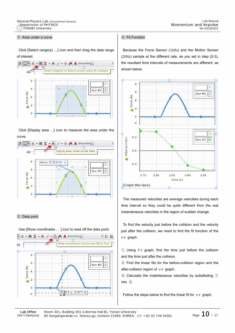
② Area under a curve

Click [Select range(s) …] icon and then drag the data range

of interest.

Click [Display area …] icon to measure the area under the

curve.

③ Data point

Use [Show coordinates … ] icon to read off the data point.

④ Fit Function

Because the Force Sensor (1kHz) and the Motion Sensor

(20Hz) sample at the different rate, as you set in step (2-3),

the resultant time intervals of measurements are different, as

shown below.

The measured velocities are average velocities during each

time interval so they could be quite different from the real

instantaneous velocities in the region of sudden change.

To find the velocity just before the collision and the velocity

just after the collision, we need to find the fit function of the

- graph.

① Using - graph, find the time just before the collision

and the time just after the collision.

② Find the linear fits for the before-collision region and the

after-collision region of - graph.

③ Calculate the instantaneous velocities by substituting ①

into ②.

Follow the steps below to find the linear fit for - graph.


Lab Manual




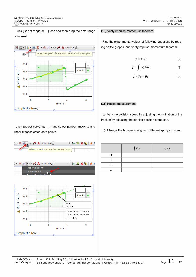
Click [Select range(s) …] icon and then drag the data range

of interest.

Click [Select curve fits … ] and select [Linear: mt+b] to find

linear fit for selected data points.

(10) Verify impulse-momentum theorem.

Find the experimental values of following equations by read-

ing off the graphs, and verify impulse-momentum theorem.

(2)

∑ (9)

(7)

(11) Repeat measurement.

① Vary the collision speed by adjusting the inclination of the

track or by adjusting the starting position of the cart.

② Change the bumper spring with different spring constant.

1

2

3

…


Lab Manual




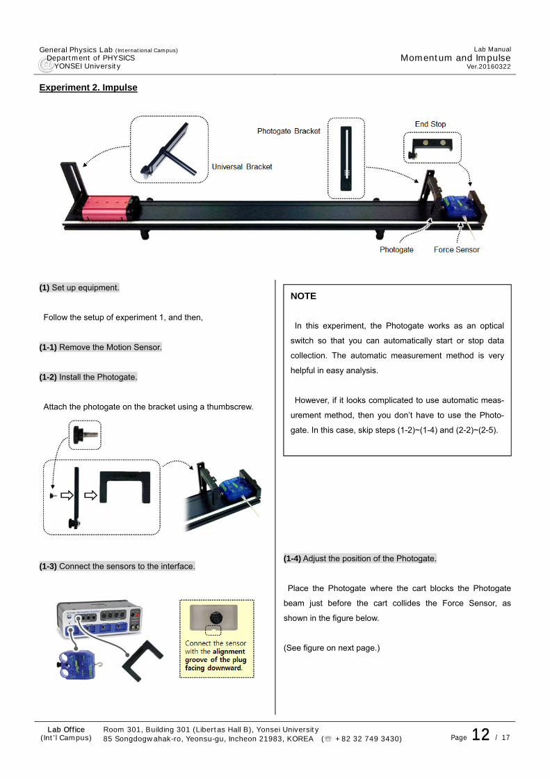
Experiment 2. Impulse

(1) Set up equipment.

Follow the setup of experiment 1, and then,

(1-1) Remove the Motion Sensor.

(1-2) Install the Photogate.

Attach the photogate on the bracket using a thumbscrew.

(1-3) Connect the sensors to the interface.

(1-4) Adjust the position of the Photogate.

Place the Photogate where the cart blocks the Photogate

beam just before the cart collides the Force Sensor, as

shown in the figure below.

(See figure on next page.)

NOTE

In this experiment, the Photogate works as an optical

switch so that you can automatically start or stop data

collection. The automatic measurement method is very

helpful in easy analysis.

However, if it looks complicated to use automatic meas-

urement method, then you don’t have to use the Photo-

gate. In this case, skip steps (1-2)~(1-4) and (2-2)~(2-5).


Lab Manual




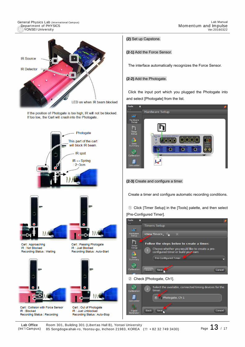
(2) Set up Capstone.

(2-1) Add the Force Sensor.

The interface automatically recognizes the Force Sensor.

(2-2) Add the Photogate.

Click the input port which you plugged the Photogate into

and select [Photogate] from the list.

(2-3) Create and configure a timer.

Create a timer and configure automatic recording conditions.

① Click [Timer Setup] in the [Tools] palette, and then select

[Pre-Configured Timer].

② Check [Photogate, Ch1].


Lab Manual




③ Select [One Photogate (Single Flag)].

④ Check [State], which outputs the value of state of the

photogate. The photogate generates ‘1’ while it is blocked,

and ‘0’ while open.

⑤ Skip steps ⑤ to ⑥ and finish the timer setup.

(2-4) Configure automatic recording conditions.

① Start Condition

The cart approaches and blocks the IR of the photogate.

The state value of the Photogate changes from ‘0’ to ‘1’.

Start data collection

② Stop Condition

The cart comes out of the Photogate after colliding with the

Force Sensor. (IR unblocked)

The state value of the Photogate changes from ‘1’ to ‘0’.

Stop data collection.

Click [Recording Conditions] in the [Controls] palette.

Select [Measurement Based] for [Condition Type] of [Start

Condition].

Set the parameters of [Start Condition] as below.

[Condition Type] : Measurement Based

[Data Source] : State()

[Condition] : Is Above

[Value] : 0.5

Set the parameters of [Stop Condition] as below.

[Condition Type] : Measurement Based

[Data Source] : State()

[Condition] : Is Below

[Value] : 0.5


Lab Manual




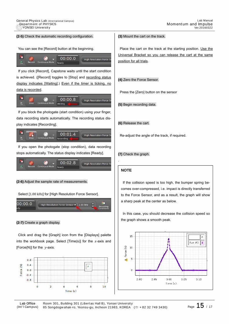
(2-5) Check the automatic recording configuration.

You can see the [Record] button at the beginning.

If you click [Record], Capstone waits until the start condition

is achieved. ([Record] toggles to [Stop] and recording status

display indicates [Waiting].) Even if the timer is ticking, no

data is recorded.

If you block the photogate (start condition) using your finger,

data recording starts automatically. The recording status dis-

play indicates [Recording].

If you open the photogate (stop condition), data recording

stops automatically. The status display indicates [Ready].

(2-6) Adjust the sample rate of measurements.

Select [1.00kHz] for [High Resolution Force Sensor].

(2-7) Create a graph display.

Click and drag the [Graph] icon from the [Displays] palette

into the workbook page. Select [Time(s)] for the -axis and

[Force(N)] for the -axis.

(3) Mount the cart on the track.

Place the cart on the track at the starting position. Use the

Universal Bracket so you can release the cart at the same

position for all trials.

(4) Zero the Force Sensor.

Press the [Zero] button on the sensor

(5) Begin recording data.

(6) Release the cart.

Re-adjust the angle of the track, if required.

(7) Check the graph.

.

NOTE

If the collision speed is too high, the bumper spring be-

comes over-compressed, i.e. impact is directly transferred

to the Force Sensor, and as a result, the graph will show

a sharp peak at the center as below.

In this case, you should decrease the collision speed so

the graph shows a smooth peak.


Lab Manual




(8) Repeat experiment using the other spring bumper.

Change the spring bumper with a different spring constant

and repeat steps (3)~(7). Make sure you do not change the

inclination of the track and the starting position of the cart so

the velocities just before collision are always same.

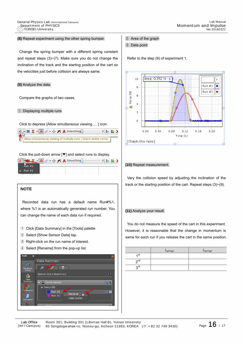
(9) Analyze the data.

Compare the graphs of two cases.

① Displaying multiple runs

Click to depress [Allow simultaneous viewing … ] icon.

Click the pull-down arrow [▼] and select runs to display.

② Area of the graph

③ Data point

Refer to the step (9) of experiment 1.

(10) Repeat measurement.

Vary the collision speed by adjusting the inclination of the

track or the starting position of the cart. Repeat steps (3)~(9).

(11) Analyze your result.

You do not measure the speed of the cart in this experiment.

However, it is reasonable that the change in momentum is

same for each run if you release the cart in the same position.

1st

2nd

3rd

NOTE

Recorded data run has a default name Run#%1,

where %1 is an automatically generated run number. You

can change the name of each data run if required.

① Click [Data Summary] in the [Tools] palette

② Select [Show Sensor Data] tap.

③ Right-click on the run name of interest.

④ Select [Rename] from the pop-up list.


Lab Manual




Your TA will inform you of the guidelines for writing the laboratory report during the lecture.

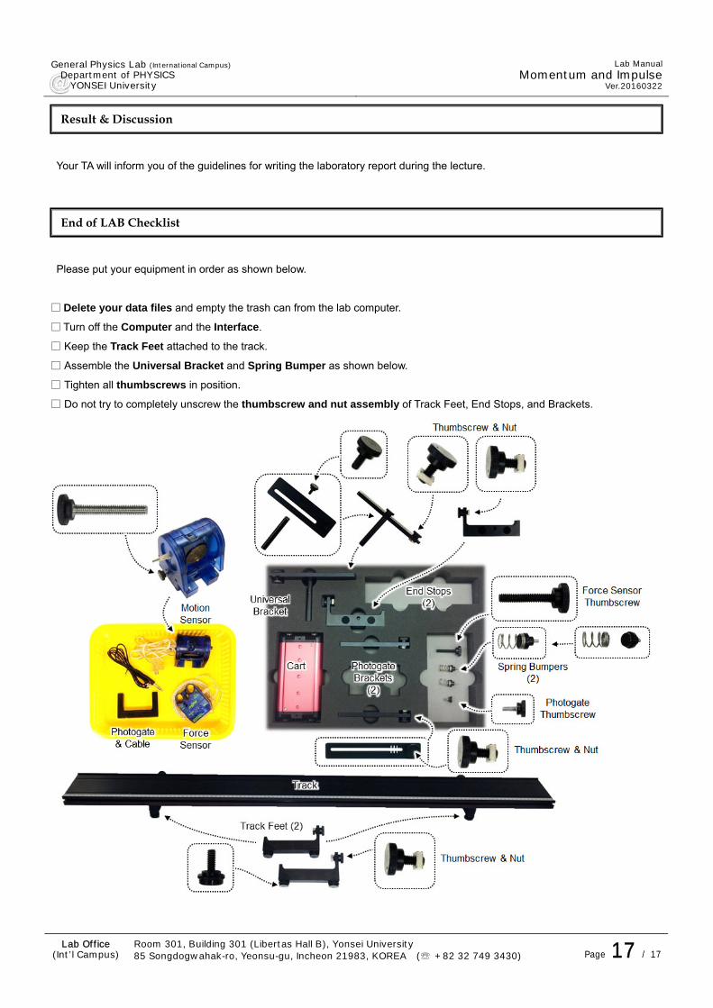
Please put your equipment in order as shown below.

□ Delete your data files and empty the trash can from the lab computer.

□ Turn off the Computer and the Interface.

□ Keep the Track Feet attached to the track.

□ Assemble the Universal Bracket and Spring Bumper as shown below.

□ Tighten all thumbscrews in position.

□ Do not try to completely unscrew the thumbscrew and nut assembly of Track Feet, End Stops, and Brackets.

Result & Discussion

End of LAB Checklist

Documents

000 Momentum ENG rev2 20160322 error삭제phylab.yonsei.ac.kr/exp_ref/104_Momentum_ENG.pdf · Momentum and Impulse Ver.20160322 Lab Office (Int’l Campus) Room 301, Building 301