Embed Size (px)
Citation preview
PHYS 705: Classical MechanicsHamiltonian Formulation &Canonical Transformation
1
Legendre TransformLet consider the simple case with just a real value function:
2
F x
expresses a relationship between an independent variable x and
its dependent value F
F x
This relation is encoded in the functional form of F x
We will denote this encoding in general by: ,F x
As one has learned in math and physics, it is sometime useful to encode the
information contained in a function in different ways…
e.g., Fourier Transform, Laplace Transform, etc.
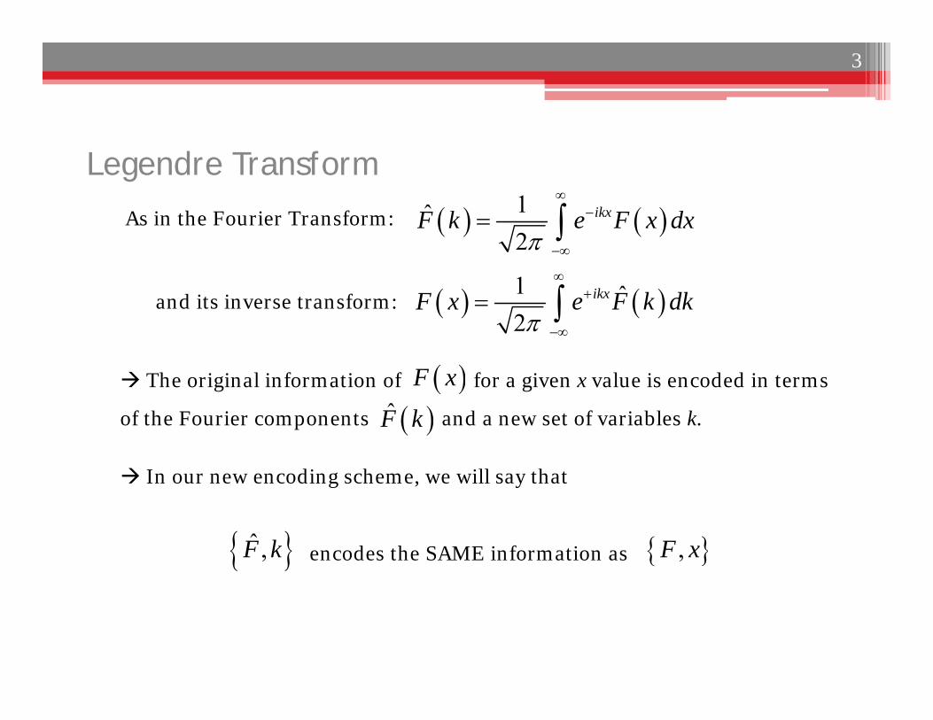
The original information of for a given x value is encoded in terms
of the Fourier components and a new set of variables k.
Legendre Transform
3
F x
In our new encoding scheme, we will say that
,F x
As in the Fourier Transform: 1ˆ2
ikxF k e F x dx
F̂ k
1 ˆ2
ikxF x e F k dk
and its inverse transform:
ˆ ,F k encodes the SAME information as
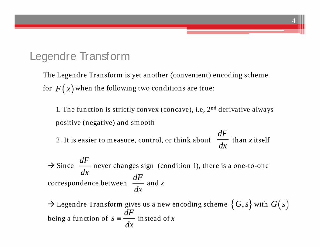
The Legendre Transform is yet another (convenient) encoding scheme
for when the following two conditions are true:
2. It is easier to measure, control, or think about than x itself
1. The function is strictly convex (concave), i.e, 2nd derivative always
positive (negative) and smooth
Legendre Transform
dFdx
4
F x
Since never changes sign (condition 1), there is a one-to-one
correspondence between and x
dFdx dF
dx
Legendre Transform gives us a new encoding scheme with
being a function of instead of x
,G s G sdFsdx
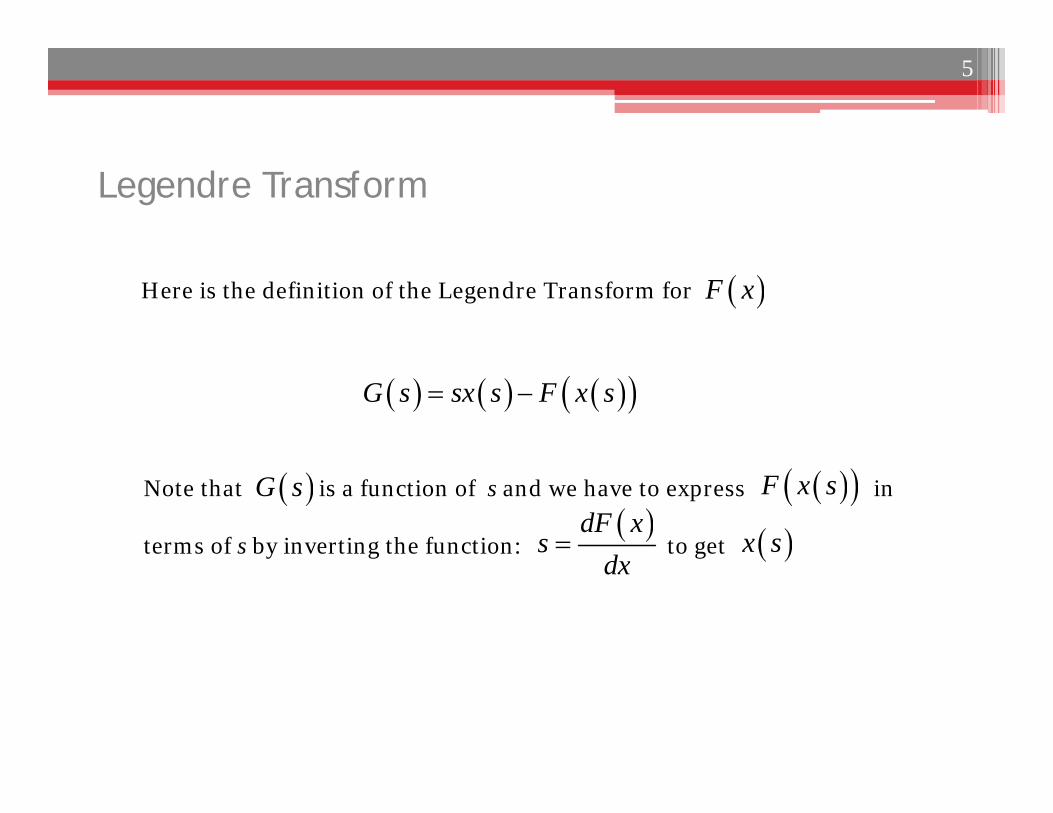
Here is the definition of the Legendre Transform for
Note that is a function of s and we have to express in
terms of s by inverting the function: to get
Legendre Transform
dF xs
dx
5
F x
G s sx s F x s
G s F x s
x s
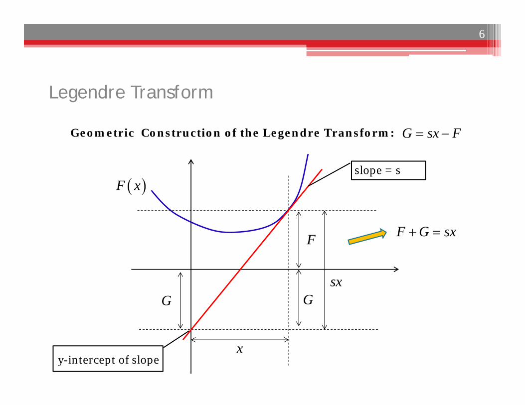
Geometric Construction of the Legendre Transform:
Legendre Transform
6
G sx F
x
F
sx
slope = s F x
GG
F G sx
y-intercept of slope
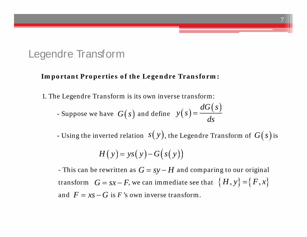
- Suppose we have and define
Important Properties of the Legendre Transform:
1. The Legendre Transform is its own inverse transform:
Legendre Transform
dG sy s
ds
7
H y ys y G s y
G s
- Using the inverted relation , the Legendre Transform of is G s s y
- This can be rewritten as and comparing to our original
transform , we can immediate see that
and is F ’s own inverse transform.
G sy H G sx F , ,H y F x
F xs G
Legendre Transform
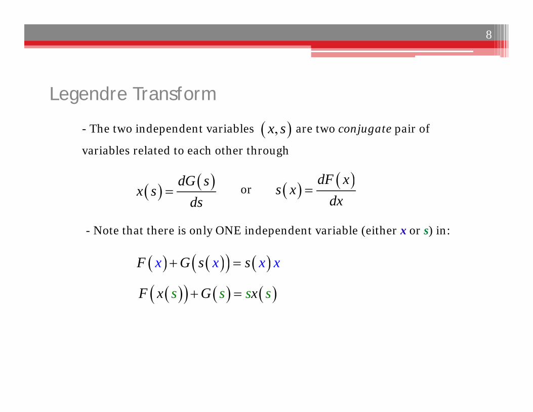
dG sx s
ds
8
- The two independent variables are two conjugate pair of
variables related to each other through
,x s
or
- Note that there is only ONE independent variable (either x or s) in:
dF xs x
dx
x x xF G s xs
s sF x G xs s
Legendre Transform
9
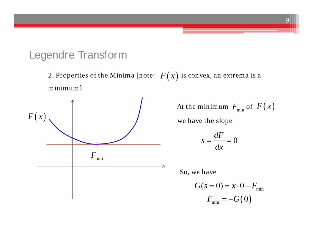
2. Properties of the Minima [note: is convex, an extrema is a
minimum]
0dFsdx
F x
minF
At the minimum of F xminFwe have the slope
So, we have
min( 0) 0G s x F
min 0F G
F x
Legendre Transform
10
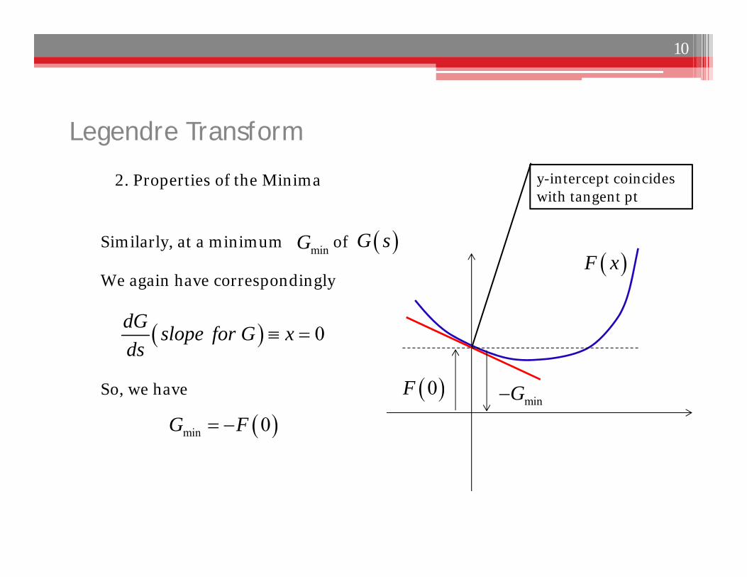
2. Properties of the Minima
minGSimilarly, at a minimum of
We again have correspondingly
min 0G F
G s
0dG slope for G xds
So, we have
F x
minG 0F
y-intercept coincides with tangent pt
Legendre Transform
11
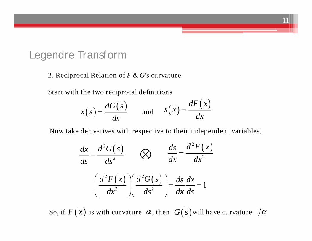
2. Reciprocal Relation of F & G’s curvature
Now take derivatives with respective to their independent variables,
dG sx s
ds
Start with the two reciprocal definitions
and dF xs x
dx
2
2
d G sdxds ds
2
2
d F xdsdx dx
2 2
2 2 1d F x d G s ds dx
dx ds dx ds
So, if is with curvature , then will have curvature F x G s 1
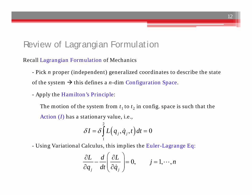
Review of Lagrangian Formulation
- Pick n proper (independent) generalized coordinates to describe the state
of the system this defines a n-dim Configuration Space.
2
1
, , 0j jI L q q t dt
Recall Lagrangian Formulation of Mechanics
0, 1, ,j j
L d L j nq dt q
- Apply the Hamilton’s Principle:
The motion of the system from t1 to t2 in config. space is such that the
Action (I) has a stationary value, i.e.,
- Using Variational Calculus, this implies the Euler-Lagrange Eq:
12
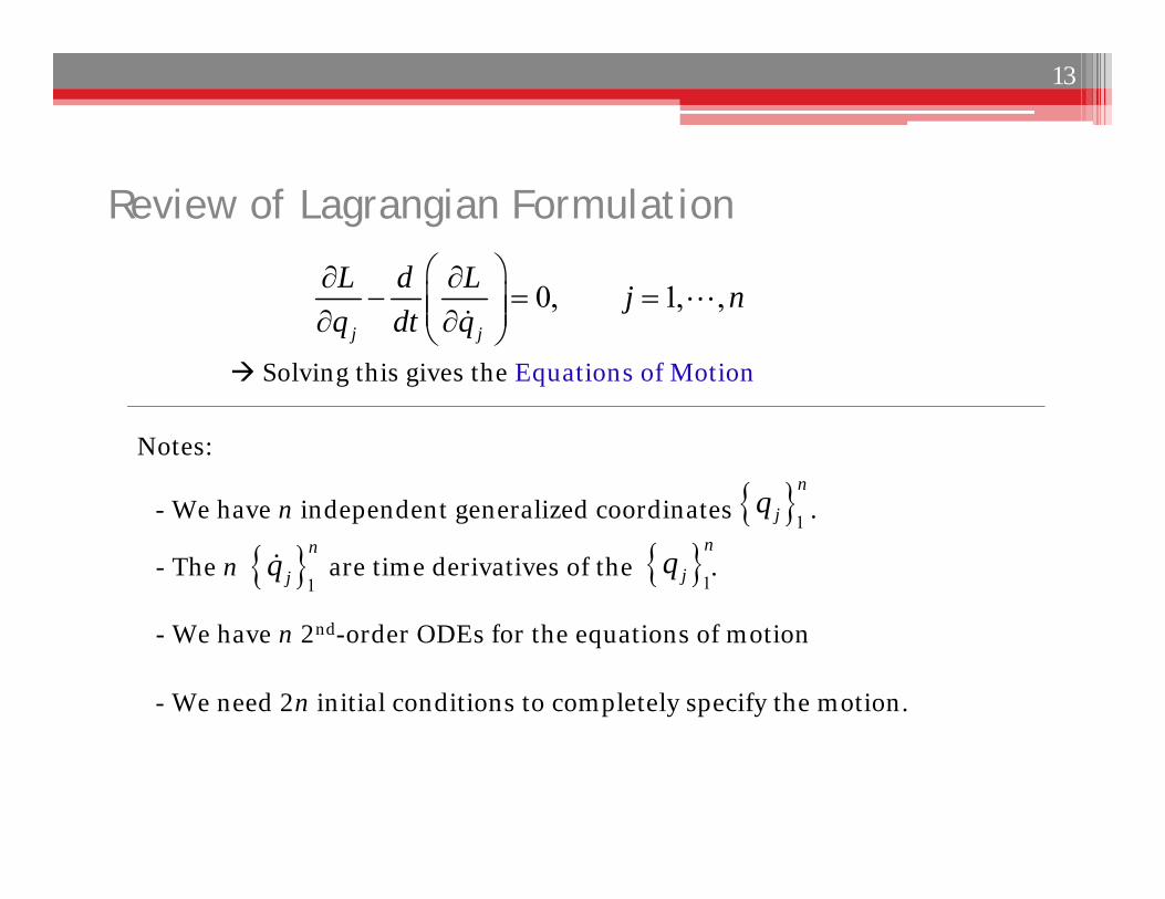
Review of Lagrangian Formulation
0, 1, ,j j
L d L j nq dt q
Notes:
- We have n independent generalized coordinates .
Solving this gives the Equations of Motion
1
n
jq
- The n are time derivatives of the . 1
n
jq
- We have n 2nd-order ODEs for the equations of motion
- We need 2n initial conditions to completely specify the motion.
1
n
jq
13
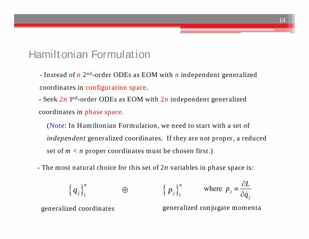
Hamiltonian Formulation
where jj
Lpq
- Instead of n 2nd-order ODEs as EOM with n independent generalized
coordinates in configuration space.
1
n
jq
(Note: In Hamiltonian Formulation, we need to start with a set of
independent generalized coordinates. If they are not proper, a reduced
set of m < n proper coordinates must be chosen first.)
1
n
jp
- The most natural choice for this set of 2n variables in phase space is:
- Seek 2n 1nd-order ODEs as EOM with 2n independent generalized
coordinates in phase space.
generalized coordinates generalized conjugate momenta
14
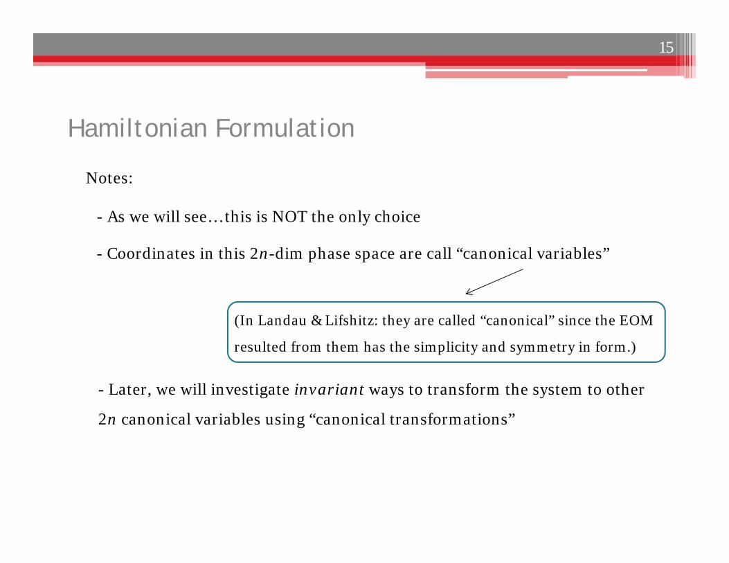
Hamiltonian Formulation
Notes:
- As we will see… this is NOT the only choice
- Coordinates in this 2n-dim phase space are call “canonical variables”
- Later, we will investigate invariant ways to transform the system to other
2n canonical variables using “canonical transformations”
(In Landau & Lifshitz: they are called “canonical” since the EOM
resulted from them has the simplicity and symmetry in form.)
15
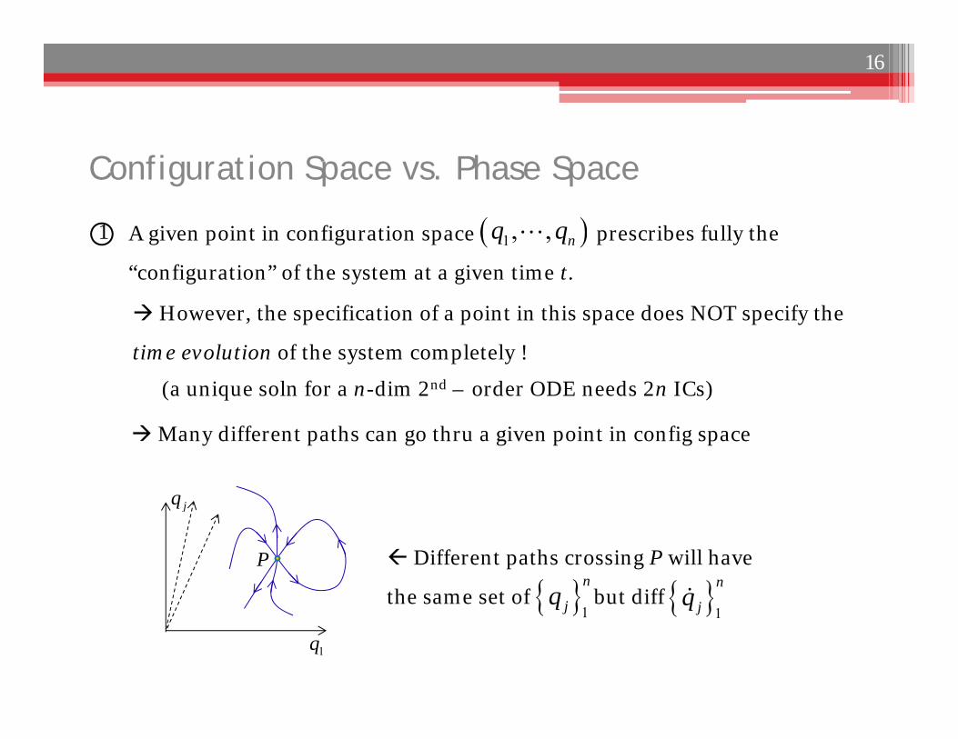
Configuration Space vs. Phase Space
A given point in configuration space prescribes fully the
“configuration” of the system at a given time t.
Different paths crossing P will have
the same set of but diff
However, the specification of a point in this space does NOT specify the
time evolution of the system completely !
1 1, , nq q
(a unique soln for a n-dim 2nd – order ODE needs 2n ICs)
Many different paths can go thru a given point in config space
1
n
jq 1
n
jq
1q
jq
P
16
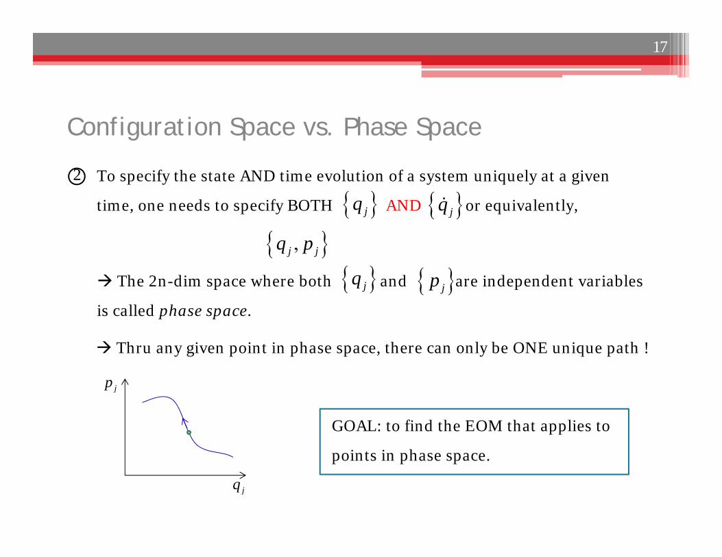
Configuration Space vs. Phase Space
To specify the state AND time evolution of a system uniquely at a given
time, one needs to specify BOTH AND or equivalently,
GOAL: to find the EOM that applies to
points in phase space.
2
,j jq p
The 2n-dim space where both and are independent variables
is called phase space.
jq jq
jq
jp
jq jp
Thru any given point in phase space, there can only be ONE unique path !
17
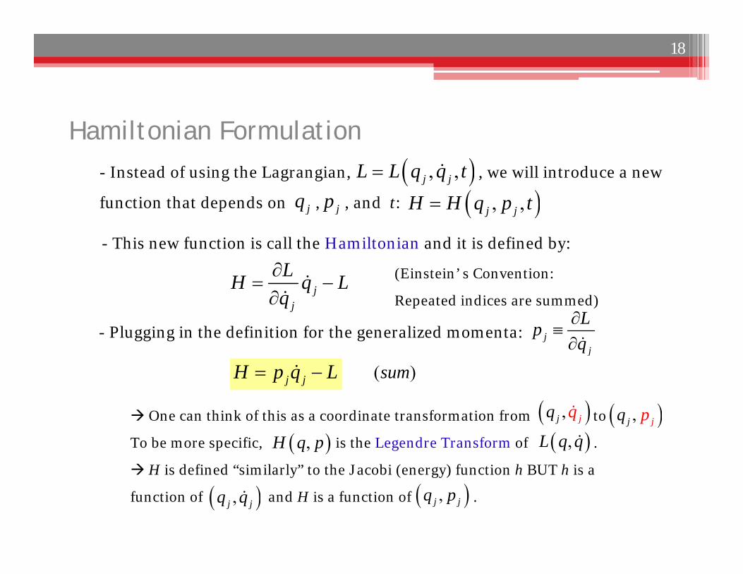
Hamiltonian Formulation- Instead of using the Lagrangian, , we will introduce a new
function that depends on , , and t:
One can think of this as a coordinate transformation from to
To be more specific, is the Legendre Transform of .
H is defined “similarly” to the Jacobi (energy) function h BUT h is a
function of and H is a function of .
, ,j jL L q q t
- This new function is call the Hamiltonian and it is defined by:
jq , ,j jH H q p tjp
- Plugging in the definition for the generalized momenta:
jj
LH q Lq
jj
Lpq
j jH p q L
, jjq q , jjq p
,j jq q ,j jq p
(Einstein’ s Convention:
Repeated indices are summed)
( )sum
,H q p ,L q q
18
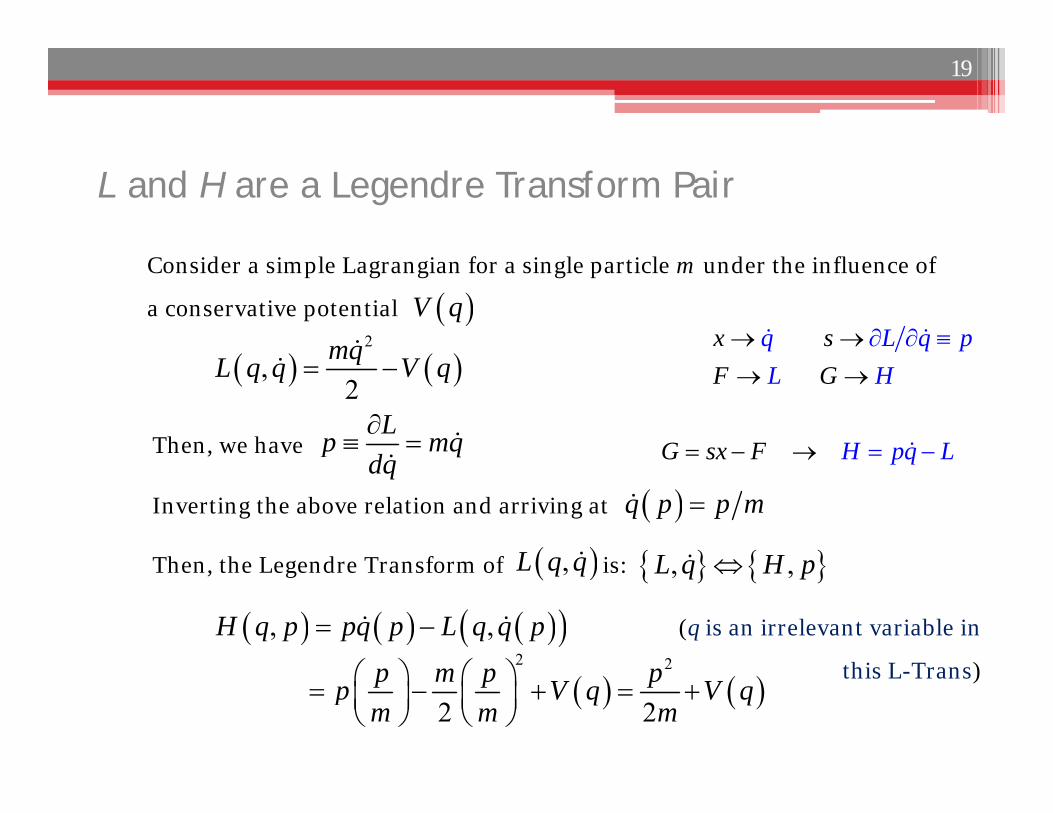
L and H are a Legendre Transform Pair
19
Consider a simple Lagrangian for a single particle m under the influence of
a conservative potential
Inverting the above relation and arriving at
Then, we haveLp mq
dq
Then, the Legendre Transform of is: ,L q q
, ,H q p pq p L q q p
2
,2
mqL q q V q
q p p m
V q
2 2
2 2p m p pp V q V qm m m
, ,L q H p
(q is an irrelevant variable in
this L-Trans)
x sF G
q L q pL H
G sx H q LF p
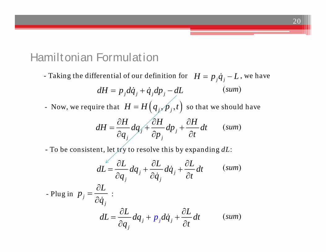
Hamiltonian Formulation- Taking the differential of our definition for , we have
- Now, we require that so that we should have
- To be consistent, let try to resolve this by expanding dL:
jj
Lpq
j j j jdH p dq q dp dL
, ,j jH H q p t
j jj j
H H HdH dq dp dtq p t
j jj j
L L LdL dq dq dtq q t
( )sum
- Plug in :
jj
jj pL LdL dq dq dtq t
( )sum
( )sum
( )sum
j jH p q L
20
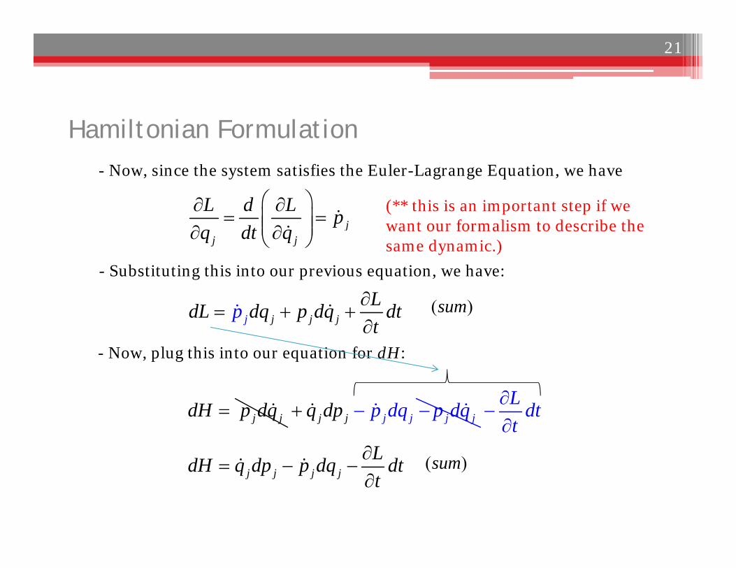
Hamiltonian Formulation- Now, since the system satisfies the Euler-Lagrange Equation, we have
- Substituting this into our previous equation, we have:
( )sum
- Now, plug this into our equation for dH:
j jj jLdL dq p dq dtt
p
jj j
L d L pq dt q
j jdH p dq jj jj j jp dd pq q qp d L dtt
j j j jLdH q dp p dq dtt
( )sum
(** this is an important step if we want our formalism to describe the same dynamic.)
21
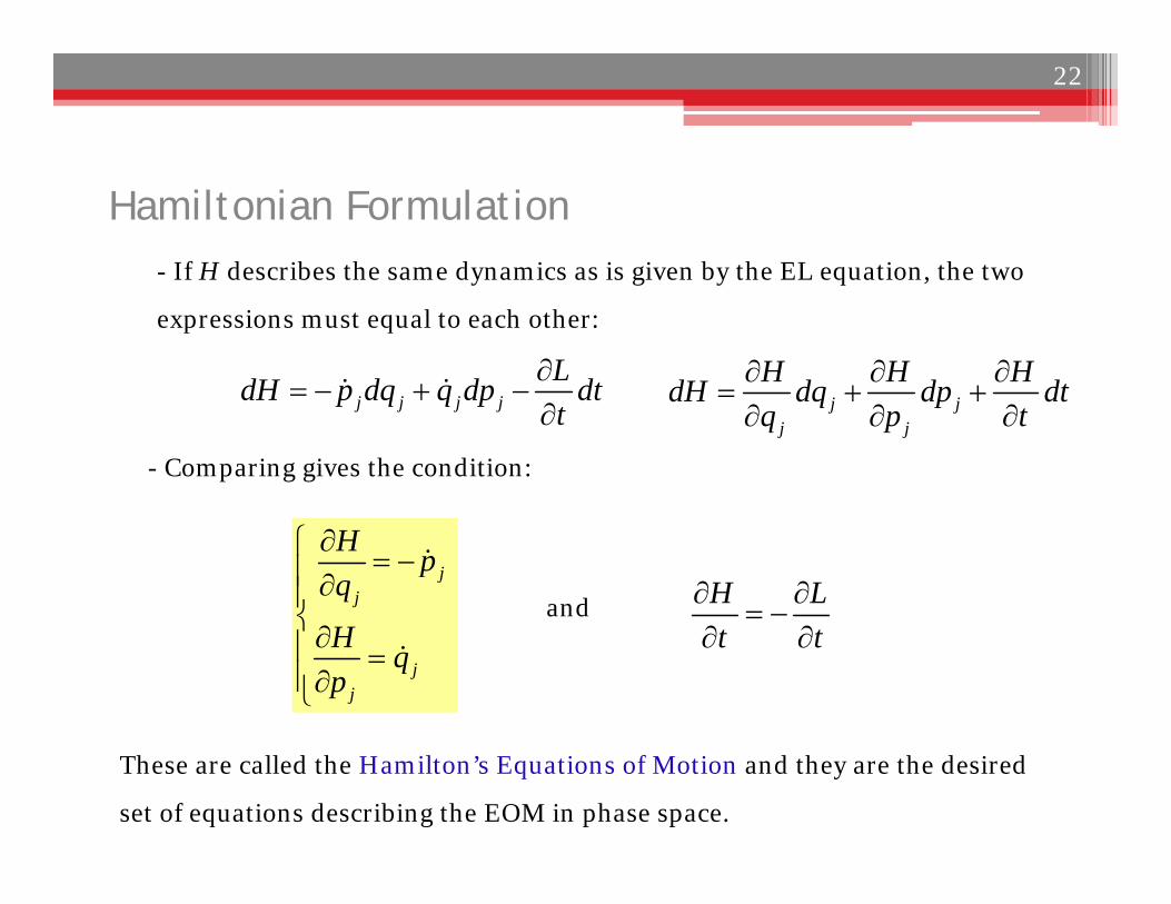
Hamiltonian Formulation- If H describes the same dynamics as is given by the EL equation, the two
expressions must equal to each other:
- Comparing gives the condition:
j j j jLdH p dq q dp dtt
j j
j j
H H HdH dq dp dtq p t
jj
jj
H pq
H qp
and H L
t t
These are called the Hamilton’s Equations of Motion and they are the desired
set of equations describing the EOM in phase space.
22
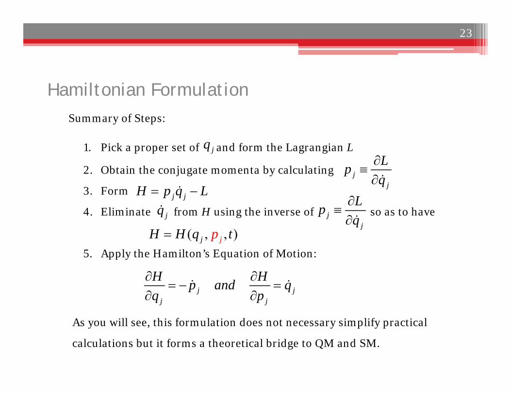
Hamiltonian FormulationSummary of Steps:
1. Pick a proper set of and form the Lagrangian L
2. Obtain the conjugate momenta by calculating
3. Form
4. Eliminate from H using the inverse of so as to have
5. Apply the Hamilton’s Equation of Motion:
jj
Lpq
As you will see, this formulation does not necessary simplify practical
calculations but it forms a theoretical bridge to QM and SM.
jq
j jH p q L
jq jj
Lpq
( , , )jj pH H q t
j jj j
H Hp and qq p
23
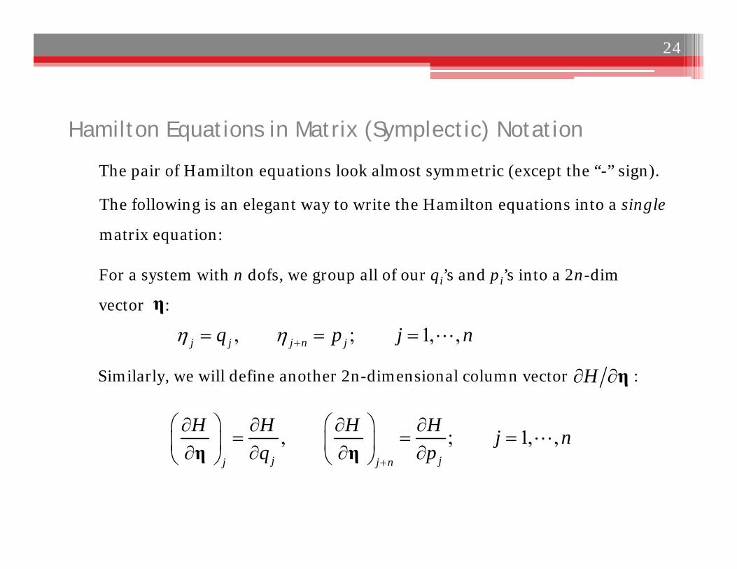
Hamilton Equations in Matrix (Symplectic) Notation
The pair of Hamilton equations look almost symmetric (except the “-” sign).
, ; 1, ,j j j n jq p j n
The following is an elegant way to write the Hamilton equations into a single
matrix equation:
, ; 1, ,j jj j n
H H H H j nq p
η η
For a system with n dofs, we group all of our qi’s and pi’s into a 2n-dim
vector :η
Similarly, we will define another 2n-dimensional column vector :H η
24
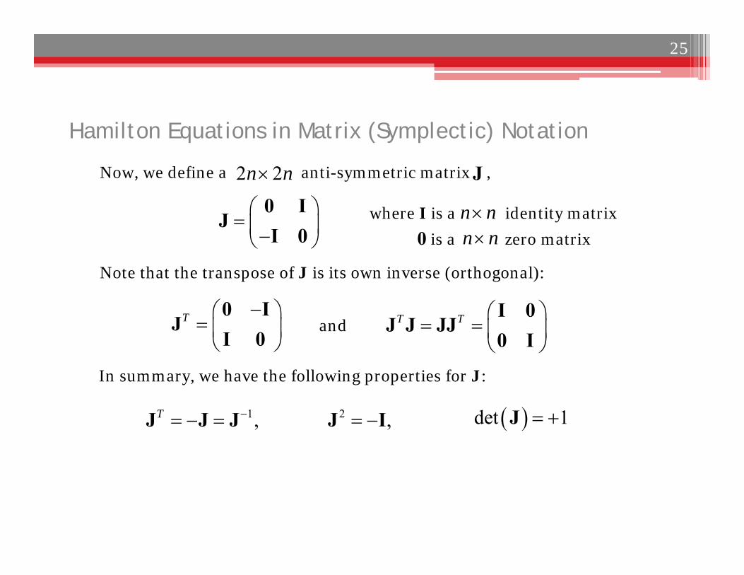
Hamilton Equations in Matrix (Symplectic) Notation
Now, we define a anti-symmetric matrix ,
Note that the transpose of J is its own inverse (orthogonal):
In summary, we have the following properties for J:
J2 2n n
0 IJ
I 0where I is a identity matrixn n
0 is a zero matrixn n
T
0 IJ
I 0T T
I 0J J JJ
0 Iand
1,T J J J 2 , J I det 1 J
25
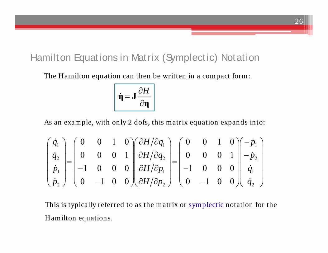
Hamilton Equations in Matrix (Symplectic) Notation
The Hamilton equation can then be written in a compact form:
1 1 1
2 2 2
1 1 1
2 2 2
0 0 1 0 0 0 1 00 0 0 1 0 0 0 11 0 0 0 1 0 0 0
0 1 0 0 0 1 0 0
q H q pq H q pp H p qp H p q
As an example, with only 2 dofs, this matrix equation expands into:
H
η J
η
This is typically referred to as the matrix or symplectic notation for the
Hamilton equations.
26
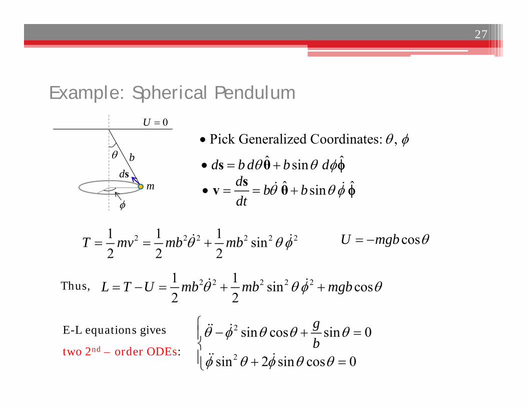
Example: Spherical Pendulum
2 2 2 2 2 21 1 1 sin2 2 2
T mv mb mb
E-L equations gives
two 2nd – order ODEs:
Pick Generalized Coordinates: , 0U
cosU mgb
2 2 2 2 21 1 sin cos2 2
L T U mb mb mgb
m
b ˆ ˆsind b d b d s θ ds
ˆ ˆsind b bdt
sv θ
Thus,
2
2
sin cos sin 0
sin 2 sin cos 0
gb
27
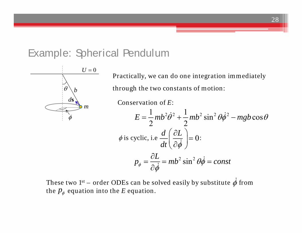
Example: Spherical Pendulum
Practically, we can do one integration immediately
through the two constants of motion:
0U
2 2 2 2 21 1 sin cos2 2
E mb mb mgb
m
bds
These two 1st – order ODEs can be solved easily by substitute from the equation into the E equation.
2 2sinLp mb const
Conservation of E:
is cyclic, i.e :0d Ldt
p
28
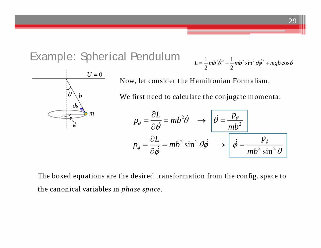
Example: Spherical Pendulum
Now, let consider the Hamiltonian Formalism.0U
m
bds
2 22 2sinsinpLp mb
mb
The boxed equations are the desired transformation from the config. space to
the canonical variables in phase space.
We first need to calculate the conjugate momenta:
22
pLp mbmb
2 2 2 2 21 1 sin cos2 2
L mb mb mgb
29
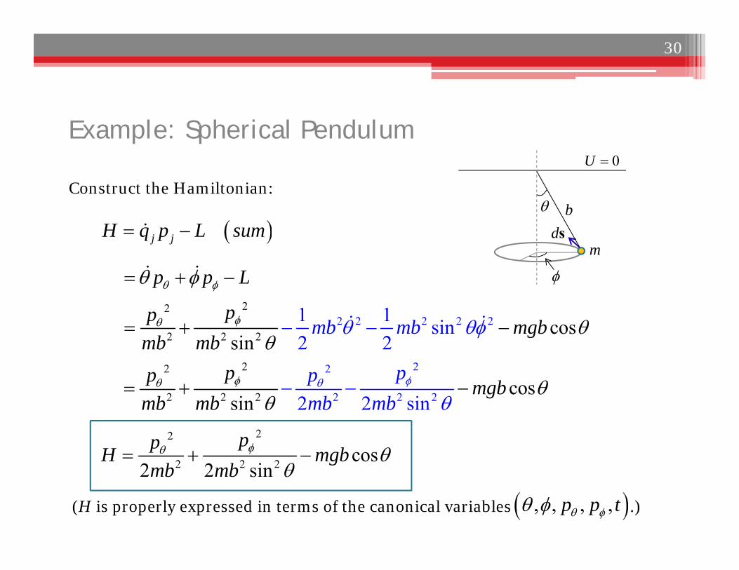
Example: Spherical Pendulum
Construct the Hamiltonian:
0U
m
bds
(H is properly expressed in terms of the canonical variables .)
j jH q p L sum
22
2 22 2 2 2 2
2 cossi
1 1 sin2n 2
mb
p p L
pp mgbmb mb
mb
22
2 2
22
2 2 22 cossi in 2 2 s n
ppm
pp mgbmb m mbb b
22
2 2 2 cos2 2 sin
ppH mgbmb mb
, , , ,p p t
30
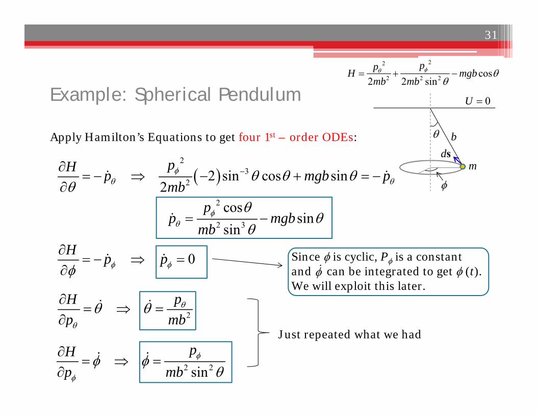
Example: Spherical Pendulum
Apply Hamilton’s Equations to get four 1st – order ODEs:
0U
m
bds
2
32 2 sin cos sin
2pH p mgb pmb
2
2 3
cossin
sinp
p mgbmb
0H p p
2
pHp mb
2 2sinpH
p mb
Just repeated what we had
Since is cyclic, P is a constant and can be integrated to get (t). We will exploit this later.
22
2 2 2 cos2 2 sin
ppH mgbmb mb
31
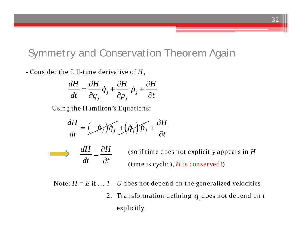
Symmetry and Conservation Theorem Again
- Consider the full-time derivative of H,
j jj j
dH H H Hq pdt q p t
Using the Hamilton’s Equations:
j jdH p qdt
j jq p Ht
dH Hdt t
(so if time does not explicitly appears in H
(time is cyclic), H is conserved!)
Note: H = E if … 1. U does not depend on the generalized velocities
2. Transformation defining does not depend on t
explicitly. jq
32
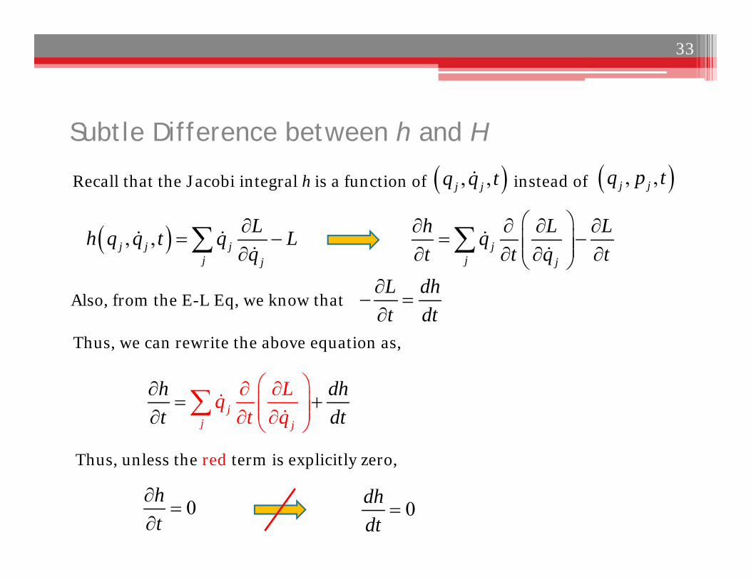
Subtle Difference between h and H
Recall that the Jacobi integral h is a function of instead of
, ,j j jj j
Lh q q t q Lq
j
j j
h L Lqt t q t
33
, ,j jq p t , ,j jq q t
Thus, we can rewrite the above equation as,
0ht
0dh
dt
Also, from the E-L Eq, we know that L dht dt
jj j
h dd
q hq tttL
Thus, unless the red term is explicitly zero,
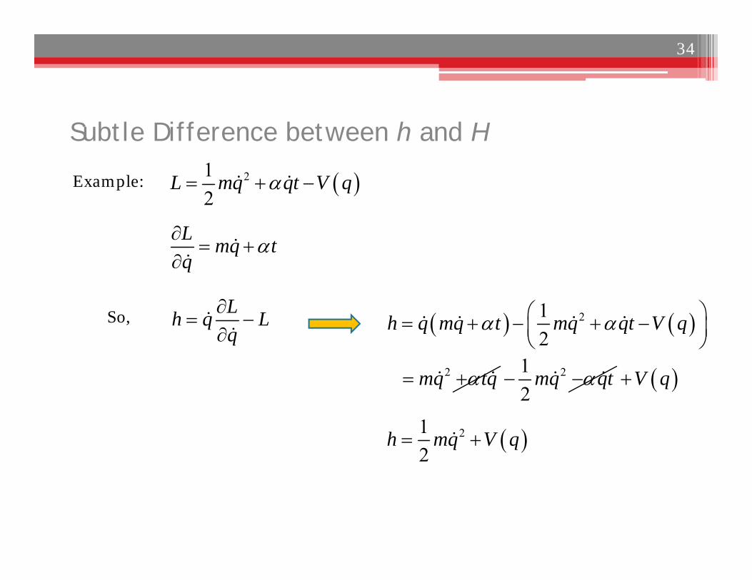
Subtle Difference between h and H
Example:
Lh q Lq
L mq tq
34
212
L mq qt V q
So, 212
h q mq t mq qt V q
2mq tq 212
mq qt V q
212
h mq V q
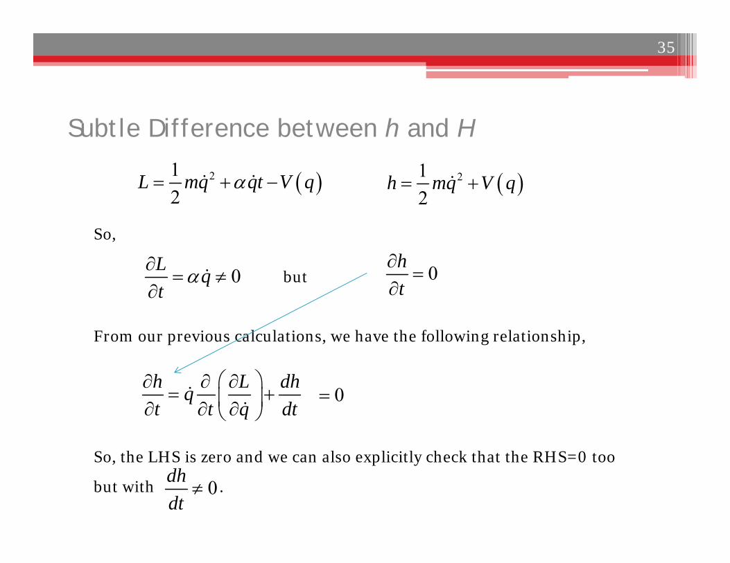
Subtle Difference between h and H
0L qt
35
212
L mq qt V q
So,
212
h mq V q
but 0ht
So, the LHS is zero and we can also explicitly check that the RHS=0 too
but with .
From our previous calculations, we have the following relationship,
h L dhqt t q dt
0
0dhdt
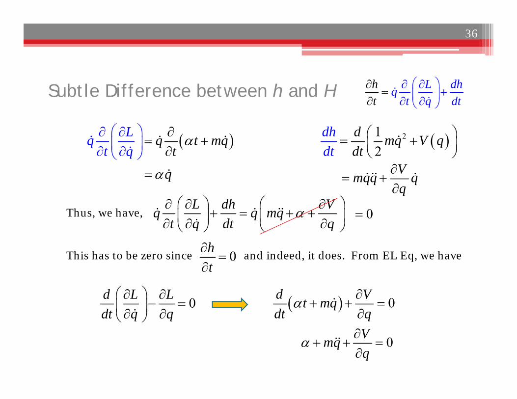
Subtle Difference between h and H
36
L dhqt
hq dtt
Lqt q
q t mqt
212
dh d m Vdt
q qdt
Vmqq qq
q
This has to be zero since and indeed, it does. From EL Eq, we have
Thus, we have,L dh Vq q mq
t q dt q
0ht
0d L Ldt q q
0d Vt mq
dt q
0Vmqq
0
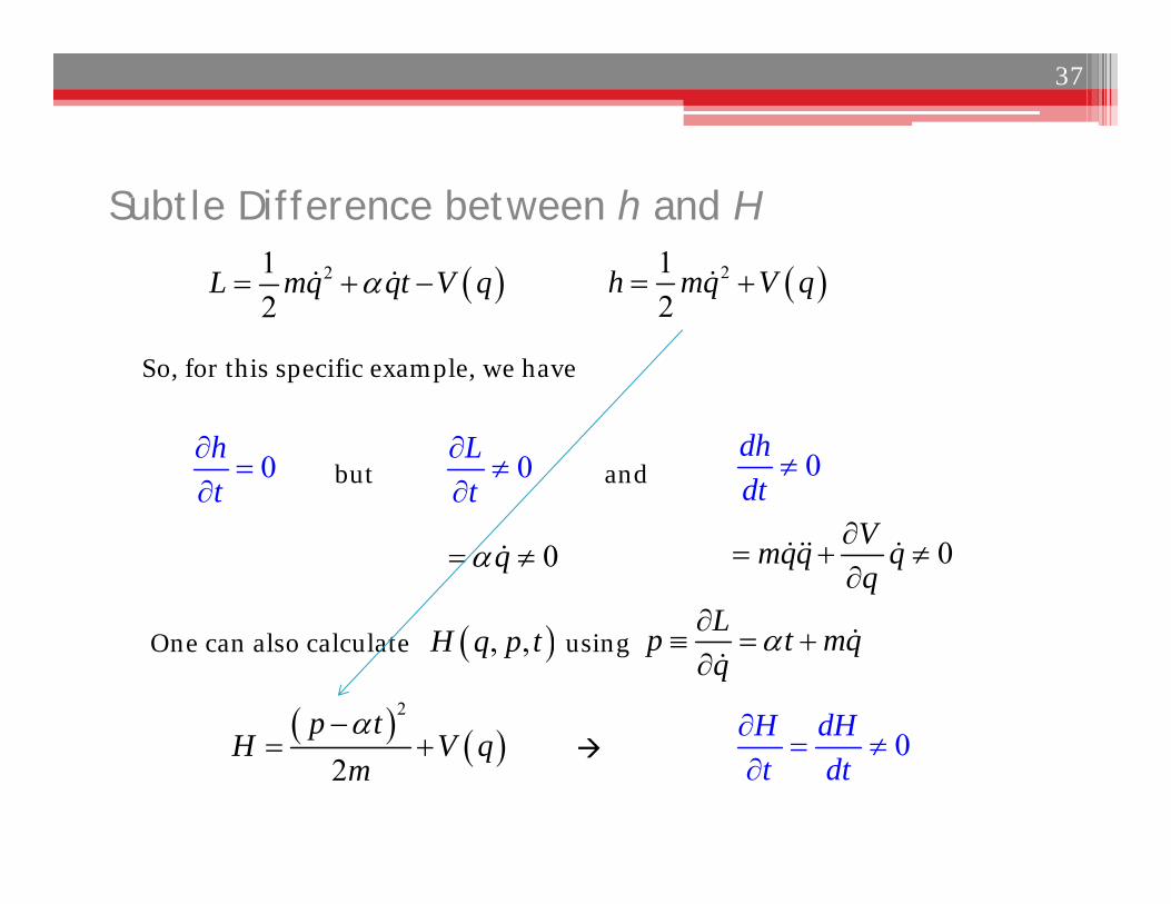
Subtle Difference between h and H
0Lt
37
212
L mq qt V q
So, for this specific example, we have
212
h mq V q
but 0ht
and 0dhdt
0Vmqq qq
0q
One can also calculate using , ,H q p tLp t mqq
2
2p t
H V qm
0H dHt dt
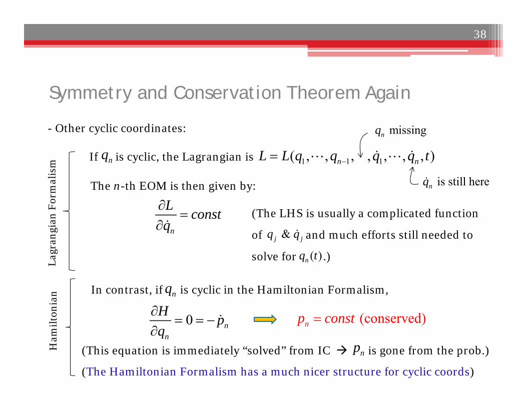
Symmetry and Conservation Theorem Again
- Other cyclic coordinates:
1 1 1( , , , , , , , )n nL L q q q q t If is cyclic, the Lagrangian is
n
L constq
(The LHS is usually a complicated function
of and much efforts still needed to
solve for .)
In contrast, if is cyclic in the Hamiltonian Formalism,
nq
missingnq
is still herenqThe n-th EOM is then given by:
& j jq q
( )nq t
Lagr
angi
an F
orm
alis
m
nq
0 nn
H pq
(conserved)np const
(This equation is immediately “solved” from IC is gone from the prob.)npHam
ilton
ian
(The Hamiltonian Formalism has a much nicer structure for cyclic coords)
38
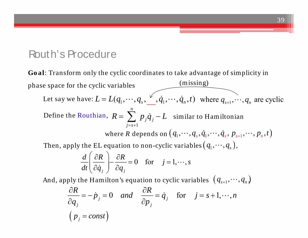
Routh’s Procedure
Goal: Transform only the cyclic coordinates to take advantage of simplicity in
phase space for the cyclic variables
1 1( , , , , , , , )s nL L q q q q t
Define the Routhian,1
n
j jj s
R p q L
where R depends on
Let say we have: 1where , , are cyclics nq q
0 for 1, ,j jj j
R Rp and q j s nq p
jp const
similar to Hamiltonian
11 1, , , , , , , , ,s s s nq q q q p p t Then, apply the EL equation to non-cyclic variables , 1, , sq q
0 for 1, ,j j
d R R j sdt q q
And, apply the Hamilton’s equation to cyclic variables , 1, ,s nq q
(missing)
39
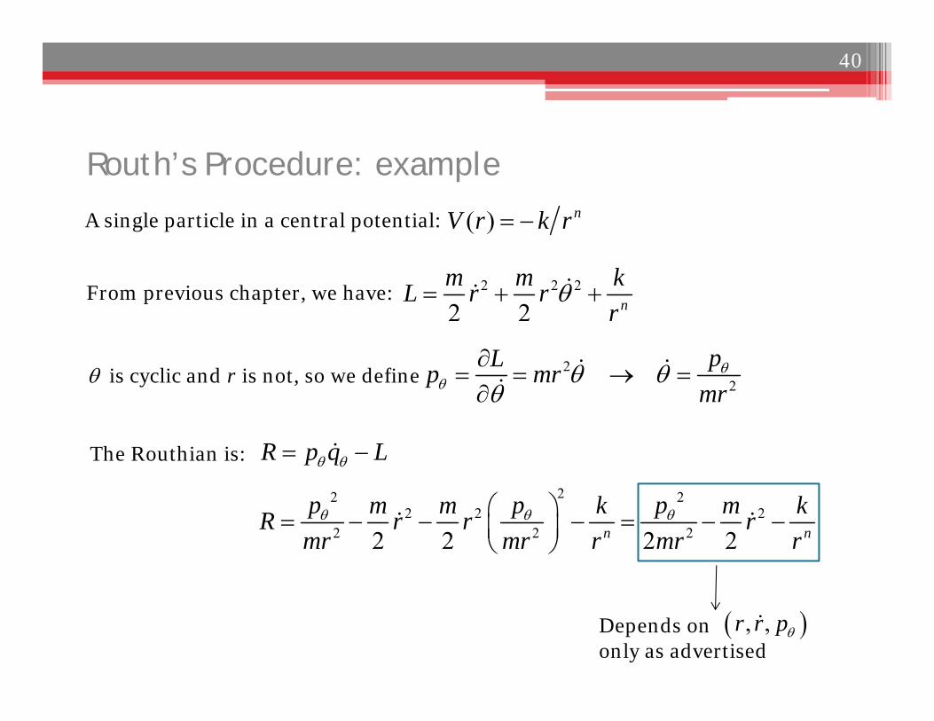
Routh’s Procedure: example
A single particle in a central potential: ( ) nV r k r
is cyclic and r is not, so we define
R p q L
From previous chapter, we have:
The Routhian is:
2 2 2
2 2 n
m m kL r rr
22
pLp mrmr
22 22 2 2
2 2 22 2 2 2n n
p p pm m k m kR r r rmr mr r mr r
Depends on only as advertised
, ,r r p
40
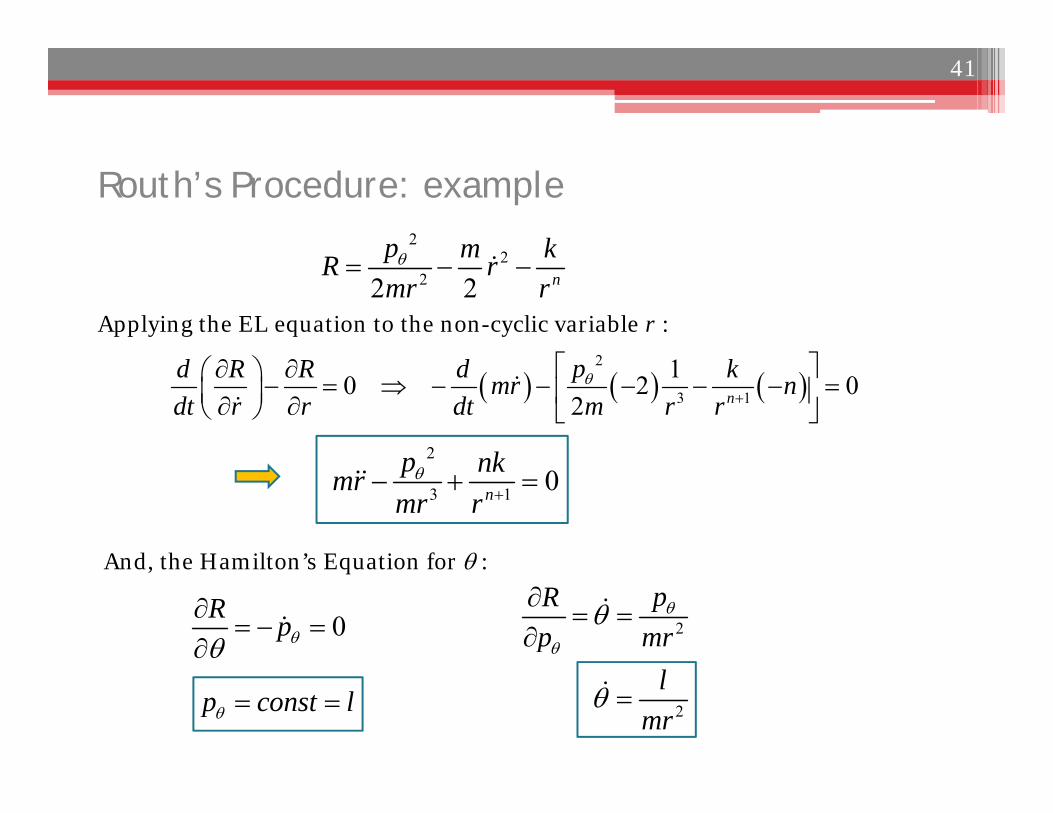
Routh’s Procedure: example
Applying the EL equation to the non-cyclic variable r :
0R p
p const l
And, the Hamilton’s Equation for :
2
3 1
10 2 02 n
pd R R d kmr ndt r r dt m r r
22
22 2 n
p m kR rmr r
2
3 1 0n
p nkmrmr r
2
pRp mr
2
lmr
41
Cyclic Variables: Action-Angle Coordinates
- Note that a given system can be described by several different sets of
generalized coordinates
Generalized coordinates are not unique !
- Recall also that the # of cyclic variables can depend on the choice of the
generalized coordinates
e.g., in the previous central force problem:
Rect coord (x, y): both x, y are not cyclic
polar coord (r, ): is cyclic
42
Cyclic Variables: Action-Angle Coordinates
- Although one might not be able to pick a set of generalized coordinates
(from a given physical system) to have ALL qj being cyclic,
Canonical Transformation (next Chapter)
one can imagine transforming them to an ideal set such that they are all
cyclic.
- If possible, then,
all the conjugate momenta are constant: j jp const
additionally, if H is a constant of motion, then
1, , nH H cannot depend on t and qj explicitly !
constant in time
cyclic
43
Cyclic Variables: Action-Angle Coordinates
consequently, the EOM for the are simple:
- Recall that the “natural” choice of the 2n-dim phase space variables is with
being the regular generalized coordinates and being their conjugate momenta.
The Hamiltonian Formalism can be extended to other possibilities:
, , , ,j j j jQ Q q p t and P P q p t
BUT, this is NOT the only choice !
1,j n jj j
H Hq func of constsp
are integration constants depending on IC
jq
( )j j jq t t j
jq
jp
(indices for are suppressed here),j jq p
44
Cyclic Variables: Action-Angle Coordinates
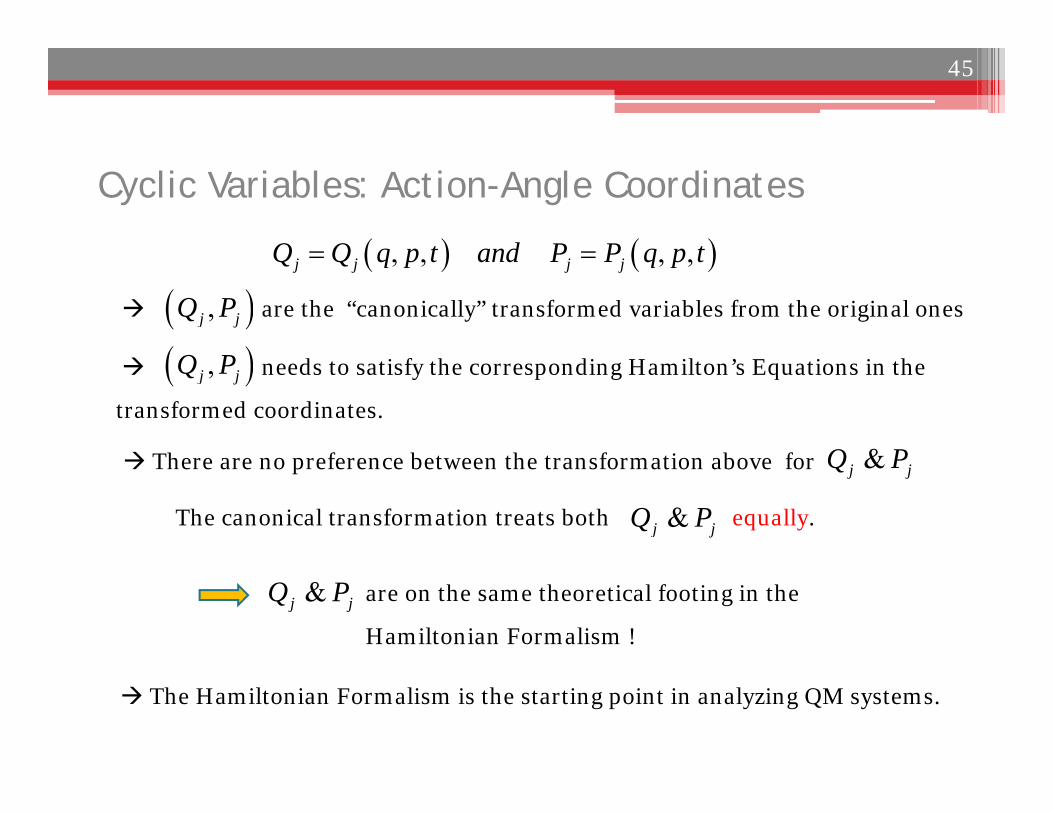
are the “canonically” transformed variables from the original ones
The canonical transformation treats both equally.
, , , ,j j j jQ Q q p t and P P q p t
are on the same theoretical footing in the
Hamiltonian Formalism !
,j jQ P
needs to satisfy the corresponding Hamilton’s Equations in the
transformed coordinates.
,j jQ P
There are no preference between the transformation above for
&j jQ P
&j jQ P
&j jQ P
The Hamiltonian Formalism is the starting point in analyzing QM systems.
45
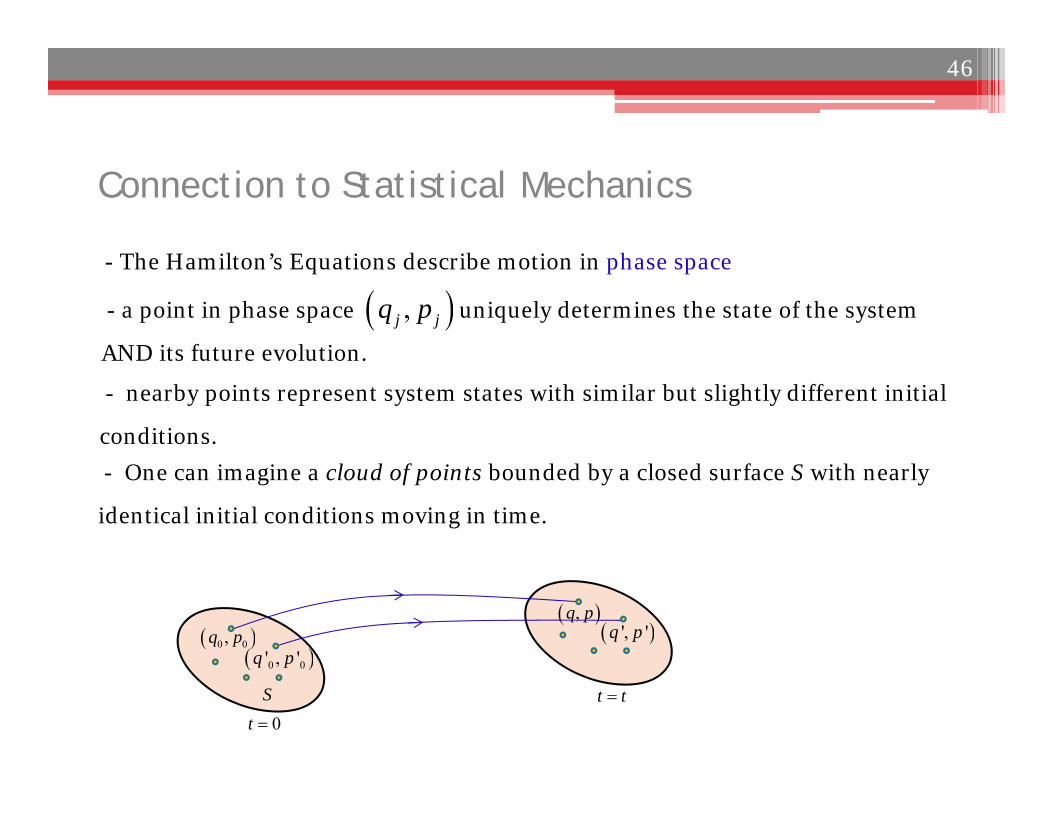
Connection to Statistical Mechanics
- The Hamilton’s Equations describe motion in phase space
- a point in phase space uniquely determines the state of the system
AND its future evolution.
,j jq p
- nearby points represent system states with similar but slightly different initial
conditions.- One can imagine a cloud of points bounded by a closed surface S with nearly
identical initial conditions moving in time.
0 0,q p 0 0' , 'q p
,q p ', 'q p
S0t
t t
46
Connection to Statistical Mechanics
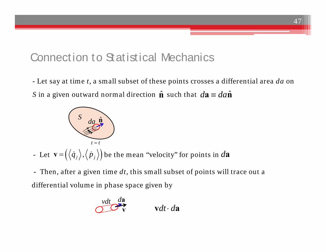
- Let say at time t, a small subset of these points crosses a differential area da on
S in a given outward normal direction such that n̂
- Let be the mean “velocity” for points in
- Then, after a given time dt, this small subset of points will trace out a
differential volume in phase space given by
t t
ˆd daa n
n̂daS
da ,j jq pv
davdtv dt dv a
47
Connection to Statistical Mechanics
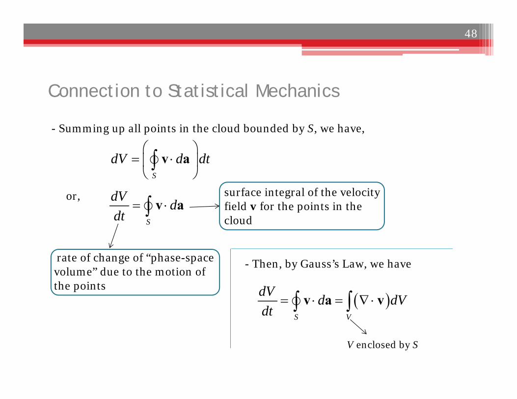
- Summing up all points in the cloud bounded by S, we have,
or,
rate of change of “phase-space volume” due to the motion of the points
S
dV d dt
v a
S
dV ddt
v asurface integral of the velocity field v for the points in the cloud
- Then, by Gauss’s Law, we have
S V
dV d dVdt
v a v
V enclosed by S
48
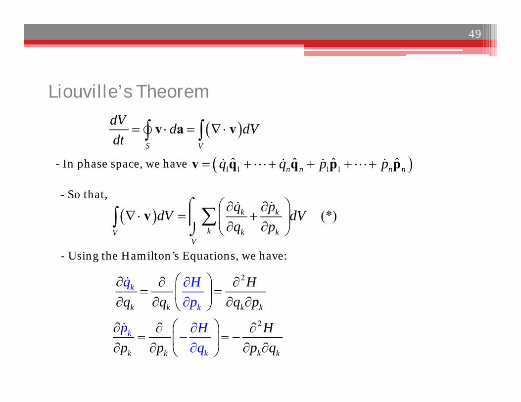
Liouville’s Theorem
- In phase space, we have
S V
dV d dVdt
v a v 1 1 1 1ˆ ˆ ˆ ˆn n n nq q p p v q q p p
- So that,
(*)k k
k k kVV
q pdV dVq p
v
- Using the Hamilton’s Equations, we have:
2
2
k k k k
k k
k
k
k k k
kq Hp
p Hq
Hq q q p
Hp p p q
49
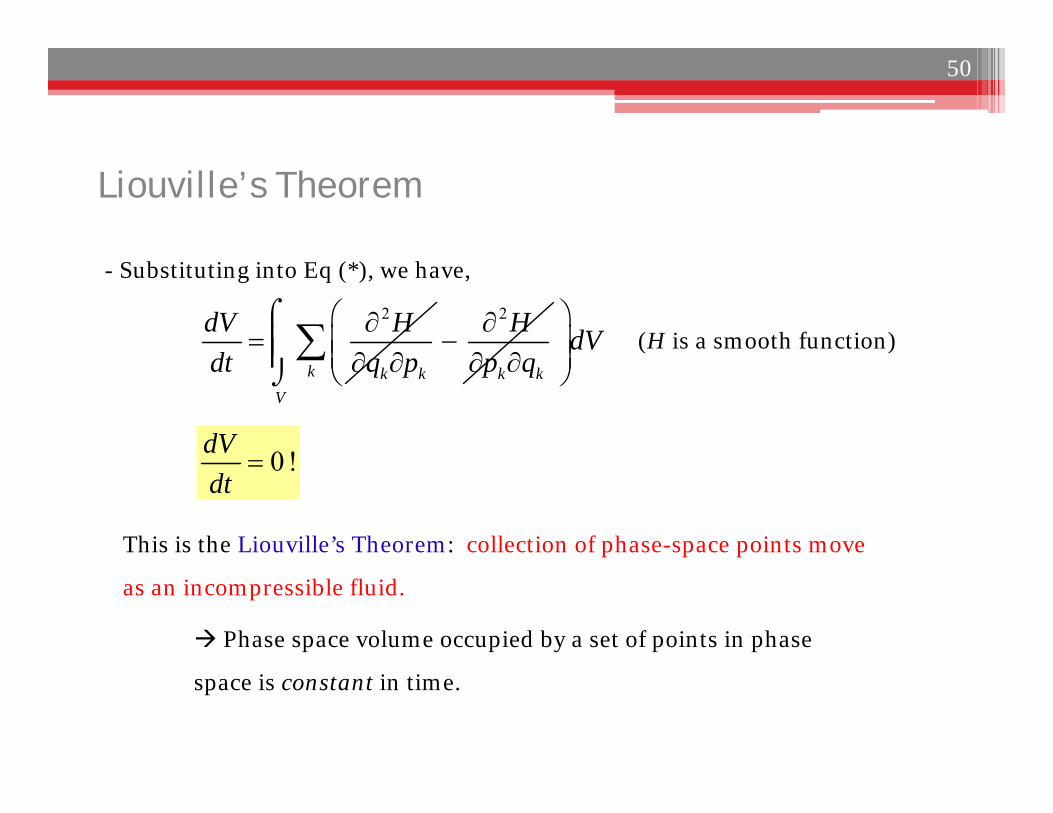
Liouville’s Theorem
- Substituting into Eq (*), we have,
2
k k
dV Hdt q p
2
k k
Hp q
k
V
dV
(H is a smooth function)
This is the Liouville’s Theorem: collection of phase-space points move
as an incompressible fluid.
0 !dVdt
Phase space volume occupied by a set of points in phase
space is constant in time.
50
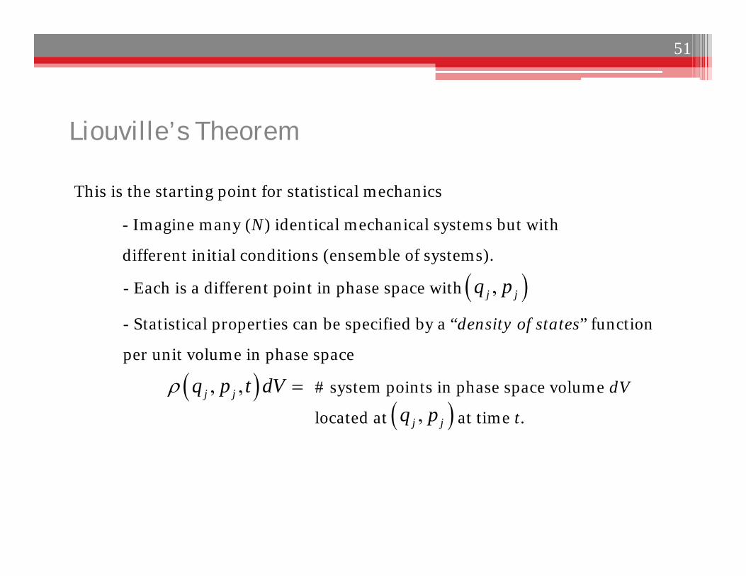
Liouville’s Theorem
This is the starting point for statistical mechanics
- Imagine many (N) identical mechanical systems but with
different initial conditions (ensemble of systems).
- Each is a different point in phase space with ,j jq p
- Statistical properties can be specified by a “density of states” function
per unit volume in phase space
, ,j jq p t dV # system points in phase space volume dV
located at at time t. ,j jq p
51
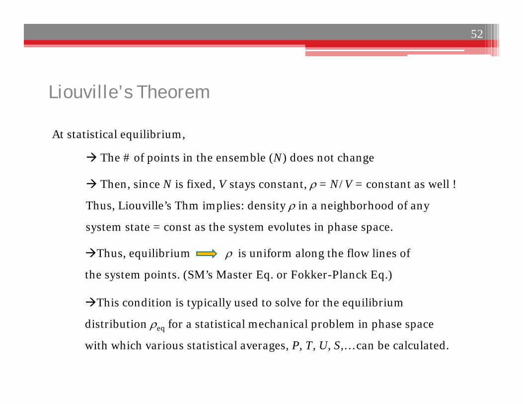
Then, since N is fixed, V stays constant, = N/V = constant as well !
Thus, Liouville’s Thm implies: density in a neighborhood of any
system state = const as the system evolutes in phase space.
Liouville’s Theorem
At statistical equilibrium,
The # of points in the ensemble (N) does not change
Thus, equilibrium is uniform along the flow lines of
the system points. (SM’s Master Eq. or Fokker-Planck Eq.)
This condition is typically used to solve for the equilibrium
distribution eq for a statistical mechanical problem in phase space
with which various statistical averages, P, T, U, S,… can be calculated.
52


![Lagrangian and Hamiltonian geometries. Applications … · arXiv:1203.4101v1 [math.DG] 19 Mar 2012 Radu MIRON Lagrangian and Hamiltonian geometries. Applications to Analytical Mechanics](https://img.pdfslide.net/doc/110x75/5b026e927f8b9a89598f9793/lagrangian-and-hamiltonian-geometries-applications-12034101v1-mathdg-19.jpg)


![[M. G. Calkin] Lagrangian and Hamiltonian Mechanic(BookZZ.org)](https://img.pdfslide.net/doc/110x75/563db7ff550346aa9a8f97ff/m-g-calkin-lagrangian-and-hamiltonian-mechanicbookzzorg.jpg)