1 / 32

Uncertainty Quantification for Chemical andBiological Hazard Assessment

Dr Ronni BowmanHazard Assessment, Simulation and Prediction Group

vbowman@dstl.gov.uk

2 / 32

Outline

• Background

• Hazard Assessment and Dispersion Modelling

• Methodology

- Sensor Placement- Source Term Estimation (STE)- Hazard Chain

• STE in Detail

• Emulation

• Uncertainty Calculation

• Uncertainty Presentation

3 / 32

Defence Science and Technology Laboratory (Dstl)

• MOD’s science and technology experts.

• Provide independent, impartial S&Tadvice to MOD and UK government.

• Not just home based. Scientists deployedto support operations.

• Work with very small companies toworld-class universities, huge defencecompanies, government departments andother nations.

• Deep and widespread research forimmediate and future requirements.

• Trading fund.

4 / 32

Dstl’s Purpose

To maximise the impact of science and technology for defence andsecurity of the UK.

• Supply sensitive and specialist science and technology services forMOD and wider government.

• Provide and facilitate expert advice, analysis and assurance to aiddecision making.

• Lead the formulation, design and delivery of a coherent andintegrated MOD science and technology programme.

• Manage and exploit knowledge across the wider defence and securitycommunity.

• Act as a trusted interface.

• Champion and develop science and technology skills across MOD.

5 / 32

Hazard Assessment

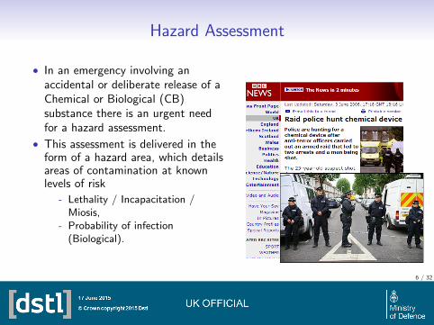
• In an emergency involving anaccidental or deliberate release of aChemical or Biological (CB)substance there is an urgent needfor a hazard assessment.

• This assessment is delivered in theform of a hazard area, which detailsareas of contamination at knownlevels of risk

- Lethality / Incapacitation /Miosis,

- Probability of infection(Biological).

6 / 32

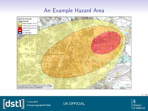
An Example Hazard Area

7 / 32

Dispersion Modelling

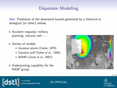
Aim: Prediction of the downwind hazard generated by a chemical orbiological (or other) release.

• Accident response; militaryplanning; volcanic ash; . . .

• Variety of models• Gaussian plume (Clarke, 1979)

• Gaussian puff (Sykes et al., 1998)

• NAME (Jones et al., 2007).

• Underpinning capability for theHASP group.

8 / 32

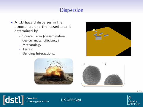
Dispersion

• A CB hazard disperses in theatmosphere and the hazard area isdetermined by

- Source Term (disseminationdevice, mass, efficiency)

- Meteorology- Terrain- Building Interactions.

9 / 32

Uncertainty

• Dispersion is highly uncertain and outputs need to be translated intoeffective information, this requires source inversion and optimization.

• Uncertainty must be propagated in order to provide a completeanswer.

• Uncertainty must be represented in a way that is understandable toa military commander.

• It has to be useful, if the uncertainty is too large it could be ignoredirrespective of the validity of the calculations.

10 / 32

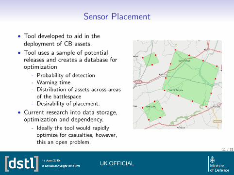
Sensor Placement

• Tool developed to aid in thedeployment of CB assets.

• Tool uses a sample of potentialreleases and creates a database foroptimization

- Probability of detection- Warning time- Distribution of assets across areas

of the battlespace- Desirability of placement.

• Current research into data storage,optimization and dependency.

- Ideally the tool would rapidlyoptimize for casualties, however,this an open problem.

11 / 32

Source Term Estimation

• Source term estimation is a highly uncertain inverse problem.

• A source term estimation model has been developed in order to inferCB source parameters from sensor readings (Robins et al. 2009).

• Inference is made by hypothesizing potential releases and calculatingtheir likelihood based on sensor readings and meteorology.

• This likelihood is then combined with various prior distributions toproduce a posterior estimate of the likely source term distribution.

• This posterior distribution is then sampled to produce a hazardestimate of where contamination is likely, based on the availabledata.

12 / 32

Source Term Estimation

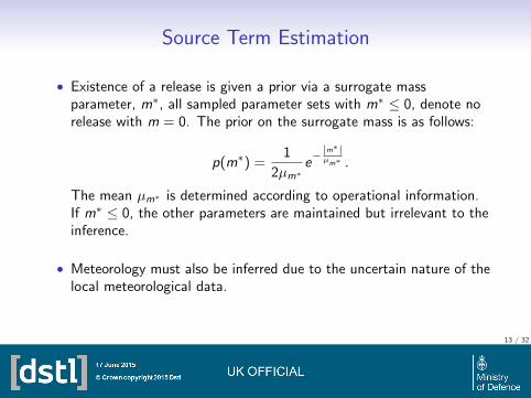
• Existence of a release is given a prior via a surrogate massparameter, m∗, all sampled parameter sets with m∗ ≤ 0, denote norelease with m = 0. The prior on the surrogate mass is as follows:

p(m∗) =1

2µm∗e−|m

∗|µm∗ .

The mean µm∗ is determined according to operational information.If m∗ ≤ 0, the other parameters are maintained but irrelevant to theinference.

• Meteorology must also be inferred due to the uncertain nature of thelocal meteorological data.

13 / 32

Source Term Estimation

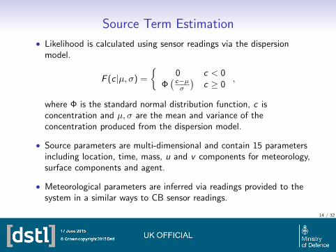
• Likelihood is calculated using sensor readings via the dispersionmodel.

F (c |µ, σ) =

{0 c < 0

Φ(

c−µσ

)c ≥ 0

,

where Φ is the standard normal distribution function, c isconcentration and µ, σ are the mean and variance of theconcentration produced from the dispersion model.

• Source parameters are multi-dimensional and contain 15 parametersincluding location, time, mass, u and v components for meteorology,surface components and agent.

• Meteorological parameters are inferred via readings provided to thesystem in a similar ways to CB sensor readings.

14 / 32

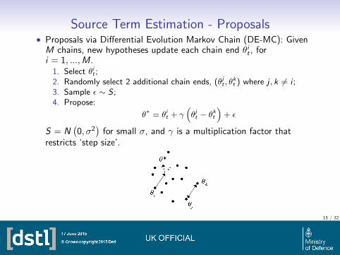
Source Term Estimation - Proposals• Proposals via Differential Evolution Markov Chain (DE-MC): GivenM chains, new hypotheses update each chain end θi

t , fori = 1, ...,M.

1. Select θit ;

2. Randomly select 2 additional chain ends, (θjt , θ

kt ) where j , k 6= i ;

3. Sample ε ∼ S ;4. Propose:

θ∗ = θit + γ

(θj

t − θkt

)+ ε

S = N(0, σ2

)for small σ, and γ is a multiplication factor that

restricts ‘step size’.

15 / 32

Source Term Estimation - Computation

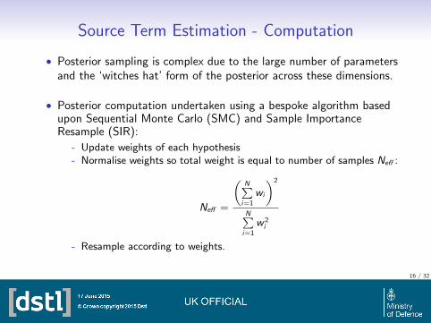
• Posterior sampling is complex due to the large number of parametersand the ‘witches hat’ form of the posterior across these dimensions.

• Posterior computation undertaken using a bespoke algorithm basedupon Sequential Monte Carlo (SMC) and Sample ImportanceResample (SIR):

- Update weights of each hypothesis- Normalise weights so total weight is equal to number of samples Neff :

Neff =

(N∑

i=1

wi

)2

N∑i=1

w 2i

- Resample according to weights.

16 / 32

Source Term Estimation - Sampling

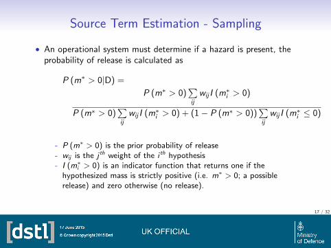
• An operational system must determine if a hazard is present, theprobability of release is calculated as

P (m∗ > 0|D) =

P (m∗ > 0)∑ij

wij I (m∗i > 0)

P (m∗ > 0)∑ij

wij I (m∗i > 0) + (1− P (m∗ > 0))∑ij

wij I (m∗i ≤ 0)

- P (m∗ > 0) is the prior probability of release- wij is the j th weight of the i th hypothesis- I (m∗

i > 0) is an indicator function that returns one if thehypothesized mass is strictly positive (i.e. m∗ > 0; a possiblerelease) and zero otherwise (no release).

17 / 32

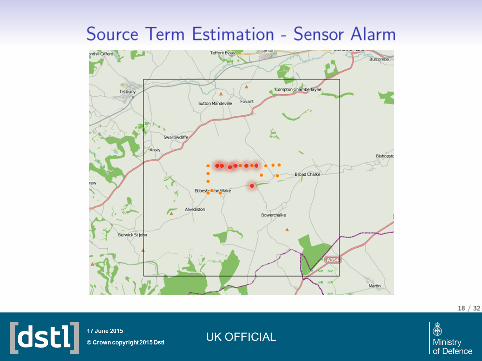
Source Term Estimation - Sensor Alarm

18 / 32

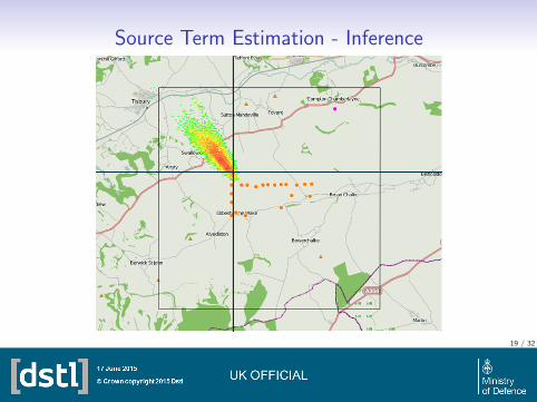
Source Term Estimation - Inference

19 / 32

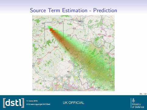
Source Term Estimation - Prediction

20 / 32

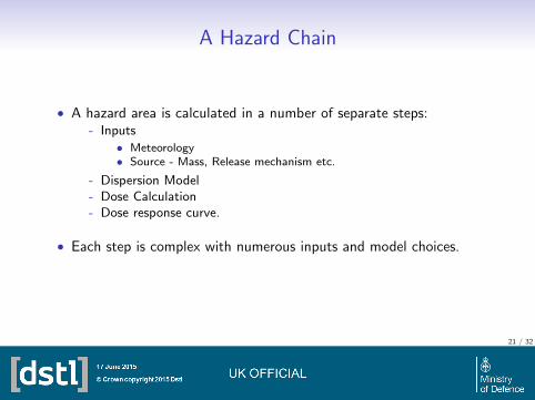
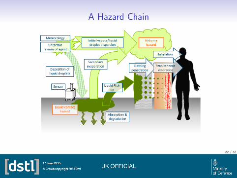
A Hazard Chain

• A hazard area is calculated in a number of separate steps:- Inputs

• Meteorology• Source - Mass, Release mechanism etc.

- Dispersion Model- Dose Calculation- Dose response curve.

• Each step is complex with numerous inputs and model choices.

21 / 32

A Hazard Chain

22 / 32

Uncertainty Quantification

• Currently the biggest limitation to accurate hazard prediction.

• Each step in the modelling chain has inherent uncertainty fromnumerous sources.

• Naively, simulation studies could be used to understand theuncertainty in predictions

- Typically models are too computationally expensive- Model inaccuracies must also be accounted for- Statistical models must be combined with real data at differing

points in the modelling chain.

• Each step is time consuming, however, answers are required in realtime.

• Uncertainty must be communicated effectively.

23 / 32

Emulation

• An initial study into the potential use of emulators focused on theemulation of the underpinning dispersion model.

• Research suggests that while emulation is possible there aresignificant challenges:

- Input parameters can result in significantly different functional output- Output is functional but also in several different forms- Meteorological and terrain constraints may require an emulator to be

developed for each location.

24 / 32

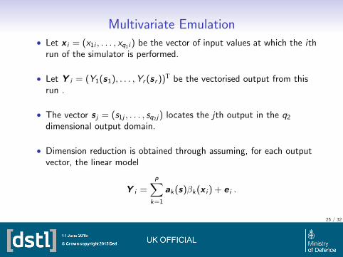
Multivariate Emulation• Let x i = (x1i , . . . , xq1i ) be the vector of input values at which the ith

run of the simulator is performed.

• Let Y i = (Y1(s1), . . . ,Yr (s r ))T be the vectorised output from thisrun .

• The vector s j = (s1j , . . . , sq2j ) locates the jth output in the q2dimensional output domain.

• Dimension reduction is obtained through assuming, for each outputvector, the linear model

Y i =

p∑k=1

ak (s)βk (x i ) + e i .

25 / 32

Multivariate Emulation

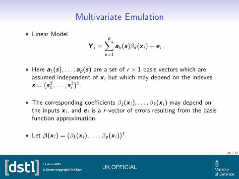
• Linear Model

Y i =

p∑k=1

ak (s)βk (x i ) + e i .

• Here a1(s), . . . , ap(s) are a set of r × 1 basis vectors which areassumed independent of x i but which may depend on the indexess = (sT

1 , . . . , sTr )T.

• The corresponding coefficients β1(x i ), . . . , βk (x i ) may depend onthe inputs x i , and e i is a r -vector of errors resulting from the basisfunction approximation.

• Let β(x i ) = (β1(x i ), . . . , βp(x i ))T.

26 / 32

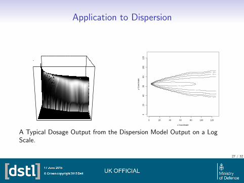
Application to Dispersion

x Coordinate

y C

oord

inat

e

0 20 40 60 80 100 120

020

4060

8010

012

0

A Typical Dosage Output from the Dispersion Model Output on a LogScale.

27 / 32

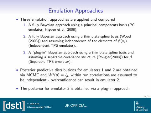
Emulation Approaches

• Three emulation approaches are applied and compared

1. A fully Bayesian approach using a principal components basis (PCemulator; Higden et al. 2008).

2. A fully Bayesian approach using a thin plate spline basis (Wood(2003)) and assuming independence of the elements of β(x i )(Independent TPS emulator).

3. A “plug-in” Bayesian approach using a thin plate spline basis andassuming a separable covariance structure (Rougier(2008)) for β(Separable TPS emulator).

• Posterior predictive distributions for emulators 1 and 2 are obtainedvia MCMC and W s(s) = Ip, within run correlations are assumed tobe independent - overconfidence can result in emulator 2.

• The posterior for emulator 3 is obtained via a plug-in approach.

28 / 32

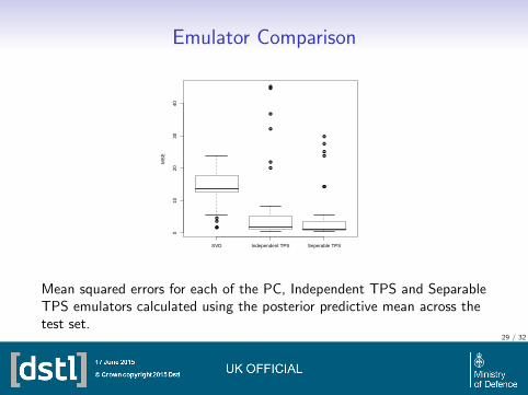
Emulator Comparison

●●

●●

●●

●

●

●

●

●

●

●

●

●

●

SVD Independent TPS Seperable TPS

010

2030

40

MS

E

Mean squared errors for each of the PC, Independent TPS and SeparableTPS emulators calculated using the posterior predictive mean across thetest set.

29 / 32

Communication

• The overall Hazard area is highly uncertain, however informationmust be conveyed in a concise and clear manner for decision makers.

• Large uncertainties can be counterproductive - a course of actionmust be obvious.

• Underestimation of the hazard area could have severe consequencesand must be avoided (over-estimation is far more acceptable withinthe bounds above).

• Spatial uncertainty is difficult to portray and this is an open problem.

30 / 32

Conclusions

• Hazard assessment is a complex problem involving:

- Multi-objective optimization of large multi-dimensional data sets.- Source Inversion under complex meteorological conditions in real

time.- Propagation of uncertainty through highly complex modelling chains

in real time with multiple uncertainty types.

• There are tools under development, however, the concatenation ofthese tools and their enhanced development are open problems.

- A method of optimization over a multi-objective, multi-dimensionalspace.

- An integrated modelling chain capable of source estimation andprediction in real time.

- Uncertainty propagation in real time through the modelling chain.

31 / 32

Selected references• Higdon, D., Gattiker, J., Williams, B. J. and Rightly, M. (2008). Journal

of the American Statistical Association 103 570-583.

• Jolliffe, I. T. (2002), 2nd ed. Springer, New York.

• Morris, M. D. and Mitchell, T. J. (1995) Journal of Statistical Planningand Inference 43 381-402.

• Rasmussen, C. E. and Williams, C. K. I. (2006). MIT Press, Cambridge,MA.

• Robins, P., Rapley, V. E. and Green, N. (2009). Journal of the RoyalStatistical Society C 58 641-662.

• Rougier, J. C. (2008). Journal of Computational and Graphical Statistics17 827-843.

• Wood, S. N. (2003). Journal of the Royal Statistical Society B 65 95-114.32 / 32

33 / 32