1

ALTERNATIVE METHODS FOR MEASURING EFFICIENCY AND AN

APPLICATION OF DEA IN EDUCATION Emmanuel Thanassoulis

Professor in Management Sciences

Aston Business School

University of Aston

Birmingham B4 7ET

Tel: +44(0) 121 3593611 Ext 5033

Fax: +44 (0) 121 359 5271

Email: e.thanassoulis@aston.ac.uk

2

PRESENTATION OUTLINE

How Data Envelopment Analysis (DEA) works in outline.

A conceptualisation of comparative efficiency measurement How Corrected and Modified OLS regression work. How Stochastic Frontier Analysis (SFA) works.

Decomposing pupil attainment between school and pupil effects using DEA.

Managerial information derived through decomposing pupil and school effects using DEA.

PART 1: OVERVIEW OF COMPARATIVE EFFICIENCY ASSESSMENT METHODS

PART 2: A REAL LIFE APPLICATION OF DEA ON BEHALF OF THE UK DEPARTMENT FOR EDUCATION AND SKILLS

3

PART 1: OVERVIEW OF COMPARATIVE EFFICIENCY ASSESSMENT METHODS

An Introduction to Efficiency and Productivity Analysis by Tim Coelli, D S Prasada Rao and George Battese (1998) Kluwer Academic Publishers (chapters 2, 3, 8, 9) ISBN: 0792380622

S.C. Kumbhakar and C.A. Knox Lovell (2000) Stochastic Frontier Analysis (Cambridge University Press) ISBN: 0521481848

Greene W H (1998) Frontier Production Functions in H. Peasaran and P. Schmidt (eds) Handbook of Applied Econometrics, volume 2, microeconomics (Blackwells)

Useful references on parametric efficiency assessment methods:

4

THE PROBLEM OF COMPARATIVE EFFICIENCY

As an integral part of managing organisations in the public and private sector we need to have information such as:

- How efficiently are the operating units using their resources?

- Is the industry such that there are economies of scale?

- Is the industry such that there are economies of scope?

- What are the efficient marginal costs of outputs;

- Has there over time been productivity change within the industry?

- How has a given operating unit fared on productivity change?

5

THE FUNDAMENTAL VIEW OF THE PROBLEM

Inputs OutputsTransformation

The units to be assessed transform inputs into outputs

The basic requirement is to compare the Decision Making Units (DMUs) on the levels of outputs they secure relative to their input levels.

6

MEASURES OF COMPARATIVE EFFICIENCY

Inputs OutputsTransformation

In a given operating context the measure of efficiency is normally one of:

- The distance between observed and maximum possible output for given inputs (output efficiency);

- The distance between observed and minimum possible input for given outputs (input efficiency);

7

There are two broad types of method for arriving at measures of comparative efficiency: parametric and non-parametric methods.

The parametric methods typically hypothesise a functional form and use the data to estimate the parameters of that function. The estimated function is then used to arrive at estimates of the efficiencies of units.

The non-parametric methods, best known as Data Envelopment Analysis (DEA), create virtual units to act as benchmarks for measuring comparative efficiency.

8

n1iexy i

Kk

1kikki

K inputs

Hypothesise a production function. E.g. the expression

PARAMETRIC METHODS FOR COMPARATIVE EFFICIENCY MEASUREMENT

Where y is output, xik are inputs, and ei is the residual for firm i.

It is the residual ei the captures any inefficiency.

Unfortunately, the residual also captures other random effects (e.g. omitted variables, measurement error, etc.) which makes it difficult to disentangle the component of inefficiency.

[1]

Two approaches exist: ignoring and not ignoring the random effects.

9

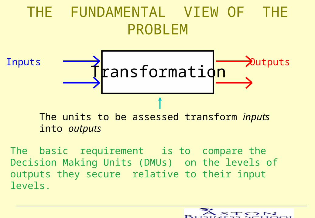
OLS regression assumes implicitly the ui have zero mean.

Let us treat the residual ei in [1] as capturing ONLY inefficiency ignoring other random effects. Then the model becomes

Now suppose we use OLS regression to estimate the model in [2].

ui >= 0.

Therefore we need to adjust the OLS model, to get the true residuals ui. Normally one of two types of adjustment is used: Corrected or Modified OLS.

n1iuxyi

Kk

1kikki

K inputs [2]

where

IGNORING RANDOM EFFECTS IN THE RESIDUAL

10

The OLS model we estimated when we assumed residual mean of zero was in effect model [2] implicitly modified to

They work as follows.

Let a* = [a-E(ui)] be the intercept of [3] that OLS regression yields. In order to retrieve the true underlying model in [2] we need to add E(ui) to a*.

The problem is that E(ui) is an estimate of the mean inefficiency of firms which we do NOT know.

1Kn

RSS

2

u =

To get an estimate of the mean inefficiency of firms we make an assumption about the theoretical probability density function of ui and then use the OLS regression residuals

to estimate . i

uE

i

uE

[3]n1i)u(Eux)u(Ey ii

Kk

1kikkii

K inputs

11

u

2uE

If ui is assumed to follow a half-normal distribution

COLS.

Adjust the intercept a* of the OLS model in [3] to

iuE*a

u

uE

Three estimates of normally are used as follows:

i

emax*a

i

uE

where ei is the residual for the ith firm in model [3] (OLS model).

MOLS - half normal

adjust the intercept a* of the OLS model in [3] to

where

If ui is assumed to follow an exponential distribution

iuE*a

MOLS - exponential

adjust the intercept a* of the OLS model in [3] to where

12

one-parameter probability density functions

0

0.5

1

1.5

2

2.5

0 1 2 3

random variable, u

f(u

)

f(u) exp f(u) half-normal

The exponential and half-normal assumption reflect the belief that larger values of inefficiency are less likely.

13

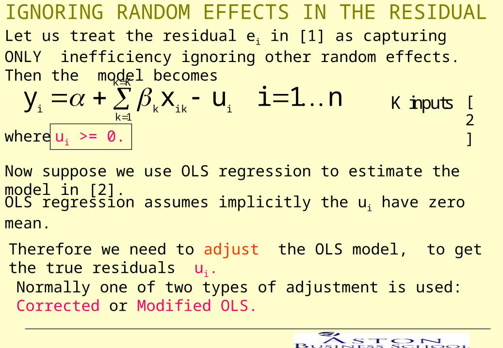
frontiers for Penn 90 data

6

7

8

9

10

11

12

5 6 7 8 9 10 11 12

log capital per worker

log

gd

p p

er w

ork

er

OLSLP/QP

COLSMOLS exp

MOLS half-normal

log gdp/worker

Illustrative application of COLS/MOLS to a set of data.

Adapted from Weyman-Jones lecture notes, Aston Business School

Inefficiency of country A: The colour of the arrow identifies the referent boundary

A

14

NOT IGNORING RANDOM EFFECTS IN THE RESIDUAL: Stochastic Frontier Analysis (SFA)

n1i]uv[xyln ii

Kk

1kikki

Key departure from COLS and MOLS is that we now have a composed error term

iiiuv

v is an identically distributed conventional two sided error term with zero mean. It stands for random noise, omitted variables etc.

u is an identically distributed one sided error term with a non-zero mean. It stands for inefficiency.u is typically assumed to be exponential, half-normal or truncated normal.

15

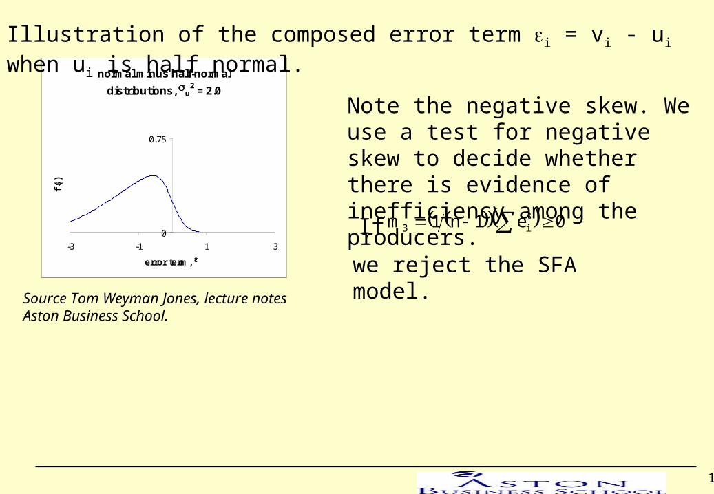
normal minus half-normal

distributions, u2 = 2.0

0

0.75

-3 -1 1 3

error term,

f()

Illustration of the composed error term i = vi - ui when ui is half normal.

Source Tom Weyman Jones, lecture notes Aston Business School.

Note the negative skew. We use a test for negative skew to decide whether there is evidence of inefficiency among the producers.

0e1n1m 3i3 If

we reject the SFA model.

16

The SFA model is usually fitted using Maximum Likelihood estimation.

We need to estimate the inefficiency of the ith producer (ui) by using its composed residual = vi - ui .

Depending on the assumption we make about the distribution of the inefficiency ui we arrive at a different formula for the conditional value

iiuE

We plug into this formula the values of and other values we derive from the to arrive at an estimate of the conditional inefficiency ui of the ith producer.

The formulae differ depending on the distribution assumed for ui but are coded in available software such as Limdep.

ii

uE

17

A GRAPHICAL OUTLINE OF THE BASIC DEA MODEL FOR ASSESSING COMPARATIVE EFFICIENCY

An introduction to Data Envelopment Analysis can be found

in:

E. Thanassoulis (2001) Introduction to the Theory and Application of

Data Envelopment Analysis: A foundation text with integrated software.

Kluwer Academic Publishers, Boston, Hardbound, ISBN 0-7923-7429-0

18

A Set of Observed Operating Units as Input -Output Correspondences

19

By virtue of interpolation between C and D all input - output correspondences on CD are feasible

20

Using interpolations between observed units the set of all feasible input -output correspondences is constructed and its boundary identified

21

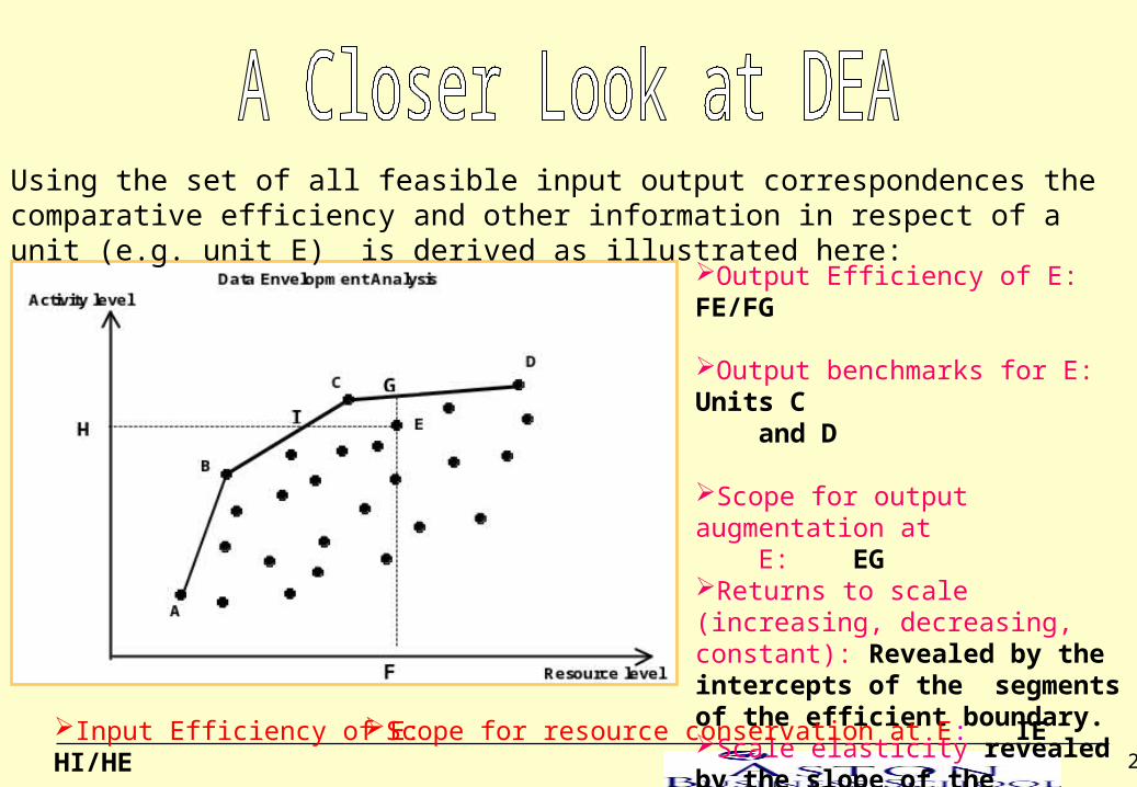
Using the set of all feasible input output correspondences the comparative efficiency and other information in respect of a unit (e.g. unit E) is derived as illustrated here:

Output Efficiency of E: FE/FG

Output benchmarks for E: Units C and D

Scope for output augmentation at E: EGReturns to scale (increasing, decreasing, constant): Revealed by the intercepts of the segments of the efficient boundary. Scale elasticity revealed by the slope of the segments on the efficient boundary.

Input Efficiency of E: HI/HE Scope for resource conservation at E: IE

22

Contrasting the Alternative Efficiency Assessment Methods All depend on identifying a

reference boundary relative to which efficiency is assessed.

DEA is non-parametric, can handle multiple inputs and outputs but assumes all distance from the boundary is inefficiency.

SFA allows for random noise in the distance from the boundary but needs assumptions on inefficiency distribution;

DEA reveals unit-specific peers, type of returns to scale, productivity change.

SFA and regression methods reveal industry level information.

COLS/MOLS can be very susceptible to outliers and do not allow for random noise.

2 4 6 8 10

2

4

6

8

10

12

0

Input

A

B

E

F

D

C G

H

DEA

OLS Regression

Output

SFA

COLS

23

PART 2: A REAL LIFE APPLICATION OF DEA ON BEHALF OF THE UK DEPARTMENT FOR EDUCATION AND SKILLS

24

Most studies measuring school performance use school level data and are parametric (regression-based).

One non - DEA approach which uses pupil - level data is One non - DEA approach which uses pupil - level data is Multi-level Modelling. It recognises the nested nature of school data (pupil within school, school within LEA etc.).

In a similar manner our approach uses pupil level data in a DEA framework to decompose pupil attainment into any number of components (pupil, school, type of school, gender etc.)

DECOMPOSING PUPIL ATTAINMENT USING DEA

It decomposes variance in pupil attainment into pupil, school etc. effects.

25

How the Decomposition Works

Take pupils in a number of schools.

We have a two-level model [pupil is level 1, school is level 2].

Any difference in attainment by pupils is as a result of a combination of: - Random Noise;- School effectiveness;- Differences in effort made by pupils.

Our approach allows for random noise and attempts to separate school from pupil effects.

26

How the Decomposition Works

BCD - Pupil-within-all-schools efficient boundary

BCH and GD Pupil- within-school efficient boundaries

OZ/OZ’ = Pupil-within-school efficiency measure of pupil Z.

OZ/OZ’’ = Pupil-within-all-schools efficiency measure of pupil Z.

0

5

10

15

20

25

30

35

40

45

20 30 40 50 60 70 80

GCSE scores

A -

leve

l sco

re

A

B

C

D

School 1

School 2

Z

Z'

Z''

O

E

F

G

H

OZ/OZ’’ = OZ/OZ’ * OZ’/OZ’’

OZ’/OZ’’ is a measure of school-within-all-schools efficiency at pupil Z

The graph shows data from school 1(dots) and school 2 (crosses)

27

Pupil-Within-All-Schools DEA efficiency =

Component attributable to pupil Component attributable to school

28

Application of the Methodology

Pupils of 122 schools who sat GCSE’s in 1992 and A or AS levels in 1994 were assessed.

DEA Input - Output Variables:

Contextual variables Outcome variables

Total GCSE points (GCSEpts) Total A and AS points (Apts)

GCSE points per attempt(GCSEpts_att)

A and AS points per attempt (Apts_att)

29

Estimation of DEA efficiencies

Given a set of n pupils, the DEA efficiency of pupil j0 relative to that set is 100/j0* % where j0* is the optimal value of in:

Max S.t.

n

j 1GCSEptsjj <= GCSEptsj0

GCSEpts_attjj < = GCSEpts_attj0

Aptsjj > = Aptsj0

Apts_attjj > = Apts_attj0

j = 1

n

j 1

n

j 1

n

j 1

n

j 1

j , 0, free

31

Decomposing Pupil-within-All Schools Efficiencies:

EFFwj0 - pupil-within-school efficiency

EFFij0 - pupil-within-all-schools efficiency EFFwj0

EFFsjo - school-within-all-schools efficiency

EFFij0 = EFFsjo * EFFwj0

32

Summary Statistics of Efficiency ScoresResults obtained considering all the pupils sampled

irrespective of school:

Mode Median Mean

Within-school efficiency (EFFwj0) 90,100 65 62.41

Within-all- schools-efficiency (EFFij0) 50,60 46.6 48.36

School-within-all schools- efficiency

(EFFsj0)

90,100 82.76 78.39

-The median pupil attains only 65% of the A-level scores of the benchmark pupil(s) in his/her own school;-The median pupil attains only 46.6% of the A-level scores of the benchmark pupil(s) across schools-The median pupils benchmark within own school attain only 82.76% of the benchmark pupils across schools.

33

Attribution of efficienciesSchool 60

0

20

40

60

80

100

Pupils

Efficiency

School 121

0

20

40

60

80

100

Pupils

Mean school-within-all-schools efficiency:

School 121 93.8%

School 60 60.56%.

34

- School 121 is more effective with stronger pupils

- School 2 is more effective with weaker pupils

Identifying Differential School Effectiveness

A school has differential effectiveness if it has a different effect on different groups of pupils.

0102030405060708090

100

2,2 3,2 4,2 5,2 6,2 7,2 8,2

GCSE points per attempt

Sch

oo

l ef

fici

ency

sco

re

School 2

School 121

GCSE points per attempt can be taken as indicative of the innate ability of a pupil

35

Pupil targets and peers

Pupils targets can incorporate several components of interest both to the pupil and to the school:

- - Within-all-schools targetsWithin-all-schools targets - A pupil can reach these - A pupil can reach these by a combination of reaching within school targets by a combination of reaching within school targets while his/her school becomes more effective. while his/her school becomes more effective. (Within-all-schools peers can indicate role model (Within-all-schools peers can indicate role model schools.)schools.)

- - Within-school targetsWithin-school targets - achievement of these - achievement of these targets depends only on the pupil. (Peers are within-targets depends only on the pupil. (Peers are within-school.)school.)

36

Other Decompositions Possible

We could in effect control for any number of categorical variables and estimate the impact of each one on pupil attainment: E.g:

Gender ( Estimate efficient boundaries within each gender and then pool the genders to compare the distance of the two boundaries.)

Type of school ( Estimate efficient boundaries within each type of school and then pool the types of school to compare the distance of the boundaries.)

Socio-economic factors ( Estimate efficient boundaries within each group of pupils (e.g. eligible v non-eligible for free school meals) and then pool the samples to compare the distance of the boundaries.)

Combinations of categorical variables (E.g. Gender and eligibility for free school meals) Estimate efficient boundaries within each combination of factors and then pool the samples to compare the distance of the boundaries.)

37

Conclusion The approach outlined recognises that pupil attainment is a

combination of various effects including effort by the pupil, the school and other categorical factors.

It can provide more complete information to schools, teachers and other parties in managing school and pupil performance. Eg:

- targets for individual pupils using other pupils within the school as benchmarks;

- targets for schools to raise their boundary closer to the inter-school boundary;- identification of any differential school effectiveness

with a view to its elimination or management.

38

Thank you