1

An attempt in modeling streamers in sprites

Hassen GhalilaLaboratoire de Spectroscopie Atomique Moléculaire et Applications

Diffuse and streamer regions of sprites : V. P. Pasko - H. C. Stenbaek-Nielsen

2

Sprites produced by quasi-electrostatic heating and ionization in the lower ionosphere V.P. Pasko, U.S. Inan, T.F. Bell and Y.N. Taranenko

Monte Carlo model for analysis of thermal runaway electrons in streamer tips in transient luminous events and streamer zones of lightning leaders

G. D. Moss, V. P. Pasko,N. Liu and G. Veronis

Effects of photoionization on propagation and branching of positive and negative streamers in sprites.

N. Liu and V. P. Pasko

References

3

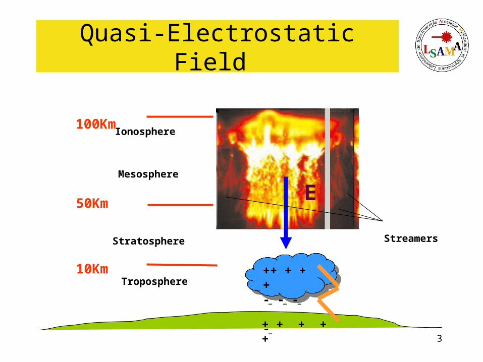
Quasi-Electrostatic Field

++ + + + - - - - - - -

++ + + + - - - - - - -

Ionosphere

Mesosphere

Stratosphere

Troposphere10Km

50Km

100Km

+ + + + +

E

Streamers

4

Geometry Schema

90Km

Perfect Conductors

60 km

Gaussian distribution

Lightning : Exponential decline of the charge Time ≈ 1ms

5

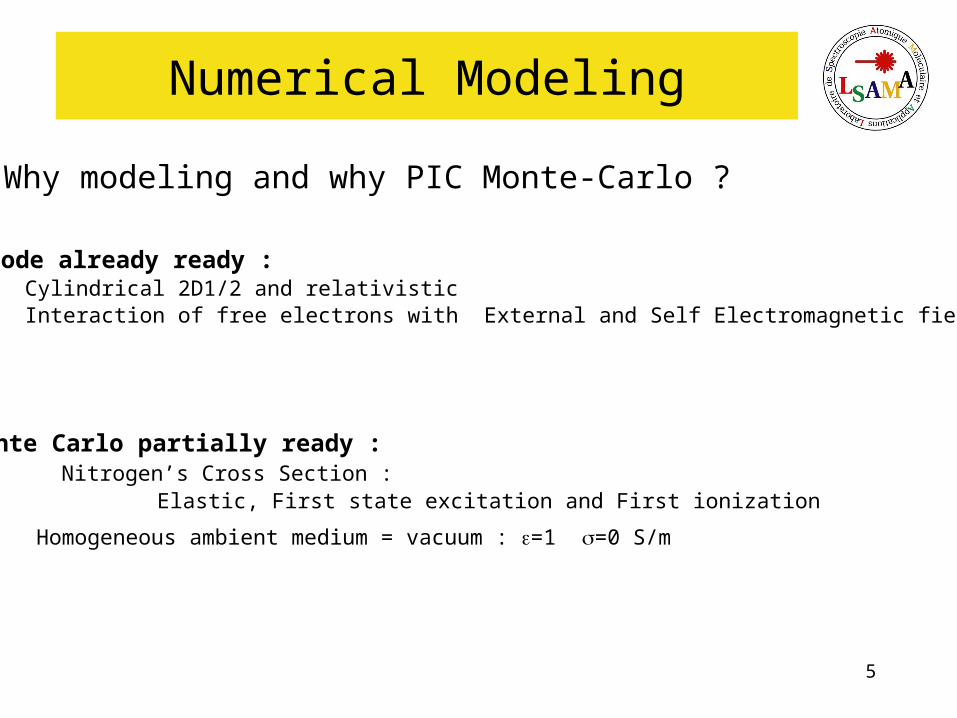
Numerical Modeling

Why modeling and why PIC Monte-Carlo ?

PIC code already ready : Cylindrical 2D1/2 and relativisticInteraction of free electrons with External and Self Electromagnetic field

Monte Carlo partially ready :Nitrogen’s Cross Section :

Elastic, First state excitation and First ionization

Homogeneous ambient medium = vacuum : =1 =0 S/m

6

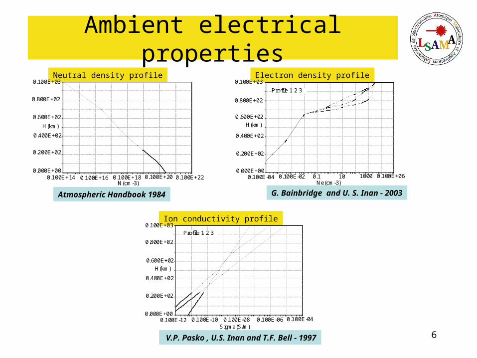
Ambient electrical properties

Ion conductivity profile

Neutral density profile Electron density profile

G. Bainbridge and U. S. Inan - 2003N(cm-3)

H(km)

0.100E+14 0.100E+16 0.100E+18 0.100E+20 0.100E+220.000E+00

0.200E+02

0.400E+02

0.600E+02

0.800E+02

0.100E+03

Ne(cm-3)

H(km)

0.100E-04 0.100E-02 0.1 10 1000 0.100E+060.000E+00

0.200E+02

0.400E+02

0.600E+02

0.800E+02

0.100E+03

Profile 1 2 3

Sigma(S/m)

H(km)

0.100E-12 0.100E-10 0.100E-08 0.100E-06 0.100E-040.000E+00

0.200E+02

0.400E+02

0.600E+02

0.800E+02

0.100E+03Profile 1 2 3

Atmospheric Handbook 1984

V.P. Pasko , U.S. Inan and T.F. Bell - 1997

7

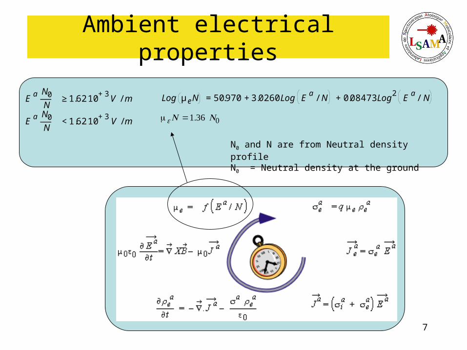
Ambient electrical properties

N0 and N are from Neutral density profileN0 = Neutral density at the ground

Log μ e N = 50.970 + 3.0260 Log Ea

/ N + 0.08473 Log2

Ea

/ N

μeN =1.36 N0

E

a N0

N≥ 1.62 10

+ 3V / m

E

a N0

N< 1.62 10

+ 3V / m

8

Expected results - Ambient E field

0

20

40

60

80

101 103 105 107

| Ez| (V/m)

0,501 s0,5 s

1 s

Ek

Altitude(km)

t = 0,5 s lightningt = 0,501 s sustained field after 1mst = 1 s relaxed field

Sprites produced by quasi-electrostatic heating and ionization in the lower ionosphere V.P. Pasko, U.S. Inan, T.F. Bell and Y.N. Taranenko

Last results

Variable constante: r = 0.000 mTrace au temps: 0.3518E+04 ns

z en m

Ez ( V/m )

0.000E+00 0.170E+05 0.340E+05 0.510E+05 0.680E+05 0.850E+051.00E+01

1.00E+03

1.00E+05

1.00E+07

Expected

9

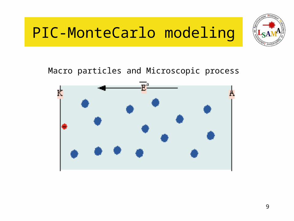
PIC-MonteCarlo modeling

Macro particles and Microscopic process

a

10

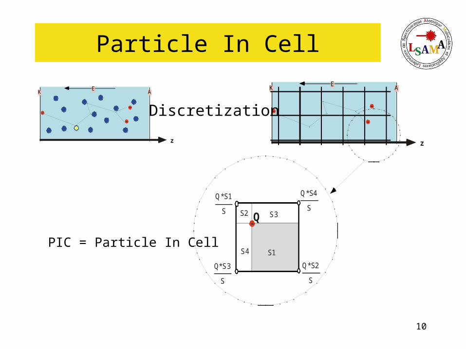
Particle In Cell

K AE

z

K AE

z

Discretization

PIC = Particle In Cell

Q

S1

Q*S1

S S2 S3

S4

Q*S2

S

Q*S4

S

Q*S3

S

11

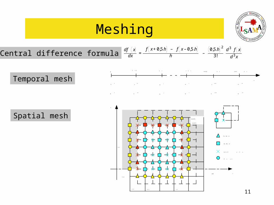
Meshing

0

t

Δ /2t Δ t n Δ t( +1/2)n Δ t

B0

P0

r1/2

E1/2

Bn

Pn

r+1/2n

E+1/2n

( +1)n Δ t

B+1n

P+1n

B1

P1

(1,2)

AXE

(1,1) (2,1)

(nzcell,

nrcell)

Er, Bz, Jr

Ez, Br, Jz

Q, U, E φ , J φ

B φ , , r z

r

z

( ,1)i

(1, )j

df x

dx=

f x+ 0,5.h – f x – 0,5.h

h–

0,5.h2

3!d 3 f x

d 3 xCentral difference formula

Temporal mesh

Spatial mesh

12

Cycle of the Calculations

Ei,j , Bi,j

E r, z , B r, z

Qr, z

Qi,j

J i,j

Interpolationdes champs

Lorentz

Collisions

Interpolationde la charge

Conservationde la charge

Maxwell

∂t B=–∇ x E

∂t E=∇x B – J

dPd t

= E + v x B ∇ . J =∂tρ

1 - ∇ . E = ρ /

2 - ∂t

B = - ∇ × E

3 - ∂t

P = ( + q E v × B )

4 - ∇ . J = ∂t

ρ

5 - μ ∂t

E = ∇ × B - μ J

4 + 5 → ∇ . E = ρ /

Coupling Maxwell-LorentzSelf-consistently

13

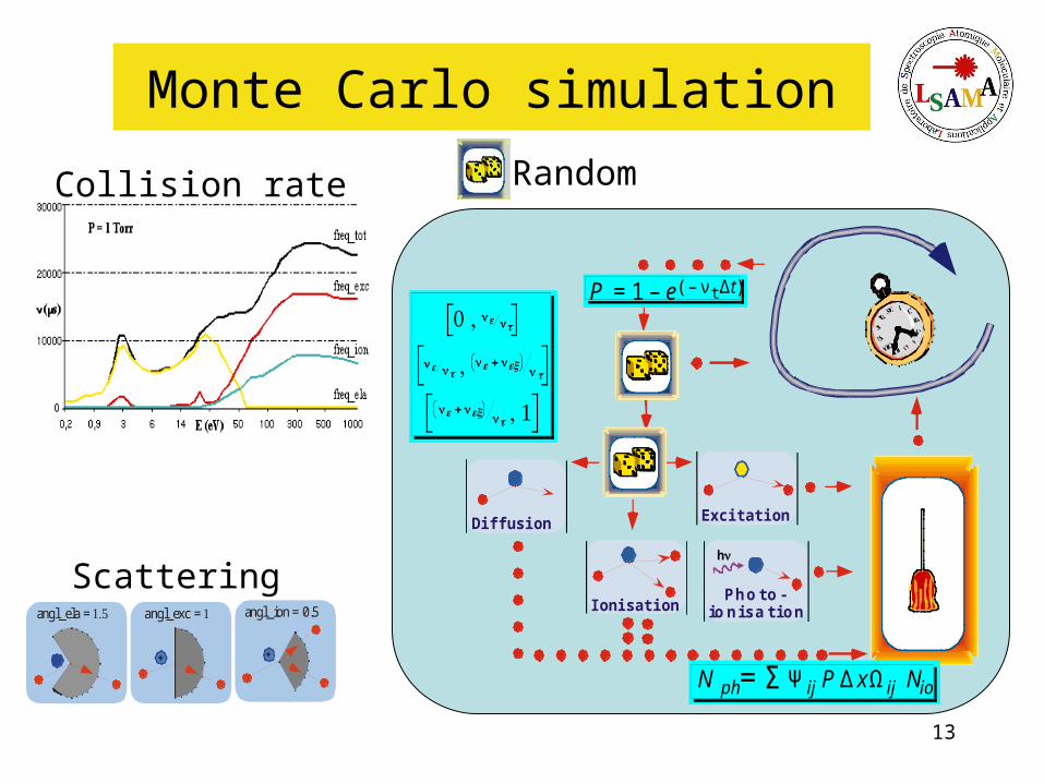
Monte Carlo simulation

Ionisation

Diffusion Excitation

Photo-ionisation

hν

0 , νe νt

νe νt

νe νtνe νt , νe+ νex ν t

νe+ νex ν t

νe+ νex νtνe+ νex νt , 1

N ph= Σ Ψ ij P Δ xΩij Nio

P = 1 – e( – ν t.Δt)

RandomCollision rate

angl_ela = 1.5 angl_ion = 0.5

+

angl_exc = 1

+

Scattering

14

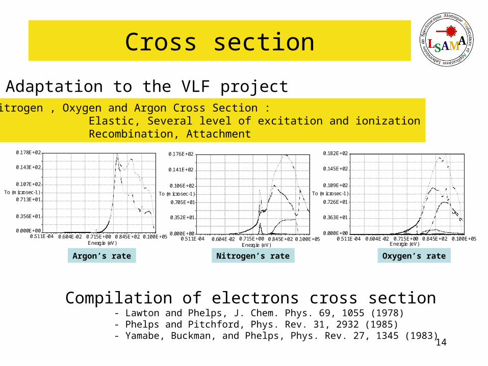
Cross section

Adaptation to the VLF projectNitrogen , Oxygen and Argon Cross Section :

Elastic, Several level of excitation and ionizationRecombination, Attachment

Argon’s rate Nitrogen’s rate Oxygen’s rate

Energie (eV)

To (microsec-1)

0.511E-04 0.604E-02 0.715E+00 0.845E+02 0.100E+050.000E+00

0.356E+01

0.713E+01

0.107E+02

0.143E+02

0.178E+02

Energie (eV)

To (microsec-1)

0.511E-04 0.604E-02 0.715E+00 0.845E+02 0.100E+050.000E+00

0.352E+01

0.705E+01

0.106E+02

0.141E+02

0.176E+02

Energie (eV)

To (microsec-1)

0.511E-04 0.604E-02 0.715E+00 0.845E+02 0.100E+050.000E+00

0.363E+01

0.726E+01

0.109E+02

0.145E+02

0.182E+02

Compilation of electrons cross section- Lawton and Phelps, J. Chem. Phys. 69, 1055 (1978)- Phelps and Pitchford, Phys. Rev. 31, 2932 (1985)- Yamabe, Buckman, and Phelps, Phys. Rev. 27, 1345 (1983)

15

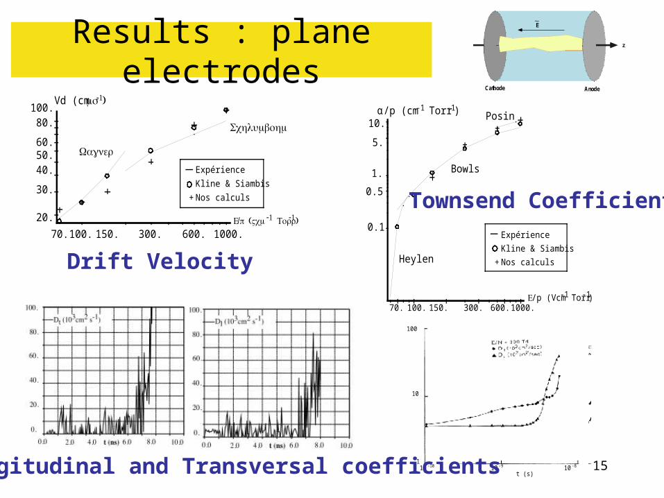
Results : plane electrodes

Expérience

Kline & Siambis

+ Nos calculs

1000.600.300.100.

100.80.

60.50.40.

30.

20.

150.70.

Vd (cm μs-1)

Wagner

Schlumbohm

Ε/ (p Vcm-1 Torr-1)

1000.600.300.100.70.

10.

5.

1.

0.5

0.1

150.Ε/p (Vcm-1 Torr-1)

α/p (cm -1 Torr -1)

Heylen

Bowls

Posin

Expérience

Kline & Siambis

+ Nos calculsDrift Velocity

Townsend Coefficient

100

10

110-10 10-9 10-8

t (s)Longitudinal and Transversal coefficients

z

Cathode Anode

E

16

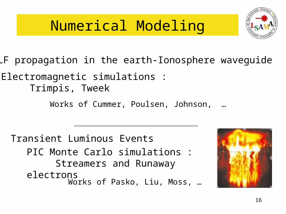
Numerical Modeling

VLF propagation in the earth-Ionosphere waveguide

Transient Luminous Events

Electromagnetic simulations :Trimpis, Tweek

Works of Cummer, Poulsen, Johnson,  …

Works of Pasko, Liu, Moss, …

PIC Monte Carlo simulations :Streamers and Runaway electrons

17

18

19

20

Brouillon

Ionospheric D region electron density profiles derived from the measured interference pattern of VLF waveguide modes G. Bainbridge and U. S. Inan

21

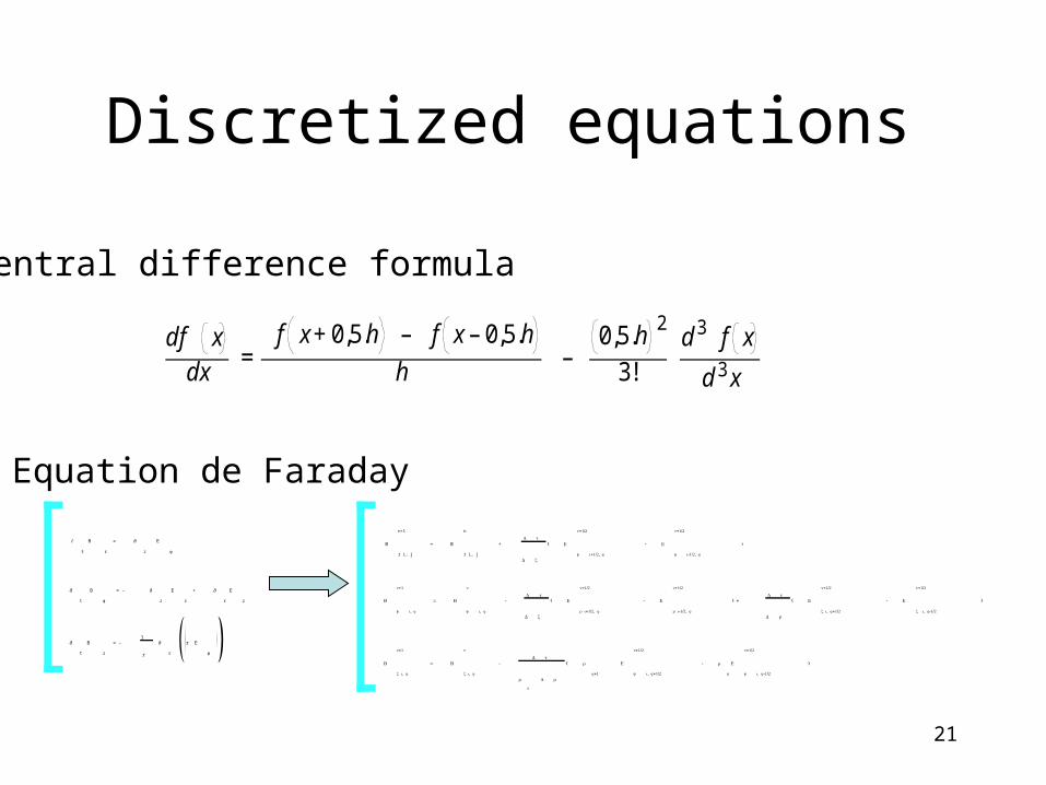
Discretized equations

∂

t

B

r

= ∂

z

E

ϕ

∂

t

B

ϕ

= - ∂

z

E

r

+ ∂

r

E

z

∂

t

B

z

= -1

r

∂

r

r E

ϕ

B

r i, j

n+1

= B

r i, j

n

+Δ t

Δ z

( E

ϕ +1/2, i j

+1/2n

- E

ϕ -1/2, i j

+1/2n

)

B

ϕ , i j

+1n

= B

ϕ , i j

n

-Δ t

Δ z

( E

+1/2, r i j

+1/2n

- E

-1/2, r i j

+1/2n

) +Δ t

Δ r

( E

, +1/2z i j

+1/2n

- E

, -1/2z i j

+1/2n

)

B

, z i j

+1n

= B

, z i j

n

-Δ t

r

0

Δ r

( r

+1j

E

ϕ , +1/2i j

+1/2n

- r

j

E

ϕ , -1/2i j

+1/2n

)

Equation de Faraday

df x

dx=

f x+ 0,5.h – f x – 0,5.h

h–

0,5.h2

3!d 3 f x

d 3 x

Central difference formula