1

Chapter 10

Introduction to Machine Learning

2

Chapter 10 Contents (1)

Training Rote Learning Concept Learning Hypotheses General to Specific Ordering Version Spaces Candidate Elimination

3

Chapter 10 Contents (2)

Inductive Bias Decision Tree Induction Overfitting The Nearest Neighbor Algorithm Neural Networks Supervised Learning Unsupervised Learning Reinforcement Learning

4

Training

Learning problems usually involve classifying inputs into a set of of classifications.

Learning is only possible if there is a relationship between the data and the classifications.

Training involves providing the system with data which has been manually classified.

Learning systems use the training data to learn to classify unseen data.

5

Rote Learning

A very simple learning method. Simply involves memorizing the

classifications of the training data. Can only classify previously seen

data – unseen data cannot be classified by a rote learner.

6

Concept Learning

Concept learning involves determining a mapping from a set of input variables to a Boolean value.

Such methods are known as inductive learning methods.

If a function can be found which maps training data to correct classifications, then it will also work well for unseen data – hopefully!

This process is known as generalization.

7

Hypotheses

A hypothesis is a vector of variables:<5, slow, red, 10, 100>

In concept learning, a training hypothesis is either a positive or negative (true or false).

A ? is used to indicate that any value will be suitable.

A Ø is used to indicate that no value will be suitable.

8

Hypotheses - Example

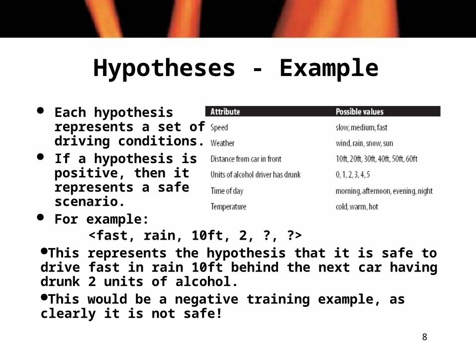
Each hypothesis represents a set of driving conditions.

If a hypothesis is positive, then it represents a safe scenario.

For example:<fast, rain, 10ft, 2, ?, ?>

This represents the hypothesis that it is safe to drive fast in rain 10ft behind the next car having drunk 2 units of alcohol.This would be a negative training example, as clearly it is not safe!

9

General to Specific Ordering This hypothesis is the most general hypothesis. It

represents the idea that it is safe to drive in any conditions:

hg = <?, ?, ?, ?, ?, ?> The following hypothesis is the most specific hypothesis: it

says it is not safe to drive in any conditions:

hs = <Ø, Ø, Ø, Ø, Ø, Ø> We can define a partial order over the set of hypotheses:

h1 >g h2

This states that h1 is more general than h2

One learning method is to determine the most specific hypothesis that matches all the training data.

10

Version Spaces

A version space is the set of hypotheses that correctly map all the training data to their categories.

A simplistic learning method would be to start from a version space of all hypotheses and to systematically remove all the ones that do not match the training data.

Clearly this would not be an efficient learning method!

11

Candidate Elimination

Candidate elimination aims to derive one hypothesis which matches all training data.

We start with a set of the most general (hg) and most specific (hs) hypotheses.

As each item of training data is examined, the set of hypotheses are modified such that all hypotheses in hs and hg match the training data.

12

Inductive Bias

All learning methods have an inductive bias.

The inductive bias of a learning method is the set of restrictions on the learning method.

Without inductive bias, a learning method could not learn to generalize.

Occam’s razor is an example of an inductive bias: The best hypothesis to select is the simplest one.

13

Decision Tree Induction (1)

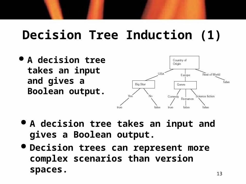
A decision tree takes an input and gives a Boolean output.

A decision tree takes an input and gives a Boolean output.

Decision trees can represent more complex scenarios than version spaces.

14

Decision Tree Induction (2)

Decision tree induction involves creating a decision tree from a set of training data that can be used to correctly classify the training data.

ID3 is an example of a decision tree learning algorithm.

ID3 builds the decision tree from the top down, selecting the features from the training data that provide the most information at each stage.

15

Decision Tree Induction (3) ID3 selects attributes based on information gain. Information gain is the reduction in entropy caused by a

decision. Entropy is defined as:

H(S) = - p1 log2 p1 - p0 log2 p0

p1 is the proportion of the training data which are positive examples

p0 is the proportion which are negative examples The entropy of S is zero when all the examples are

positive, or when all the examples are negative. The entropy reaches its maximum value of 1 when

exactly half of the examples are positive, and half are negative.

16

The Problem of Overfitting

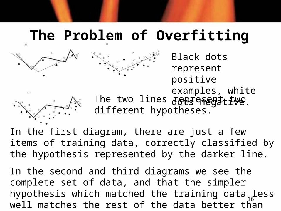
Black dots represent positive examples, white dots negative.

The two lines represent two different hypotheses.

In the first diagram, there are just a few items of training data, correctly classified by the hypothesis represented by the darker line.

In the second and third diagrams we see the complete set of data, and that the simpler hypothesis which matched the training data less well matches the rest of the data better than the more complex hypothesis, which overfits.

17

The Nearest Neighbor Algorithm (1)

This is an example of instance based learning.

Instance based learning involves storing training data and using it to attempt to classify new data as it arrives.

The nearest neighbor algorithm works with data that consists of vectors of numeric attributes.

Each vector represents a point in n-dimensional space.

18

The Nearest Neighbor Algorithm (2)

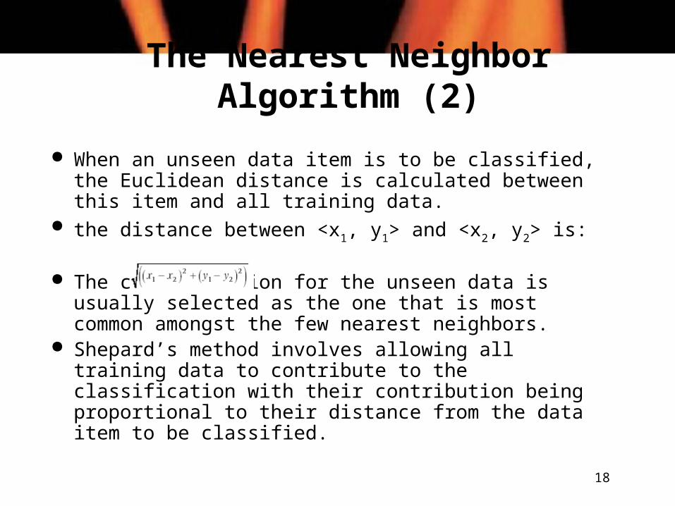
When an unseen data item is to be classified, the Euclidean distance is calculated between this item and all training data.

the distance between <x1, y1> and <x2, y2> is:

The classification for the unseen data is usually selected as the one that is most common amongst the few nearest neighbors.

Shepard’s method involves allowing all training data to contribute to the classification with their contribution being proportional to their distance from the data item to be classified.

19

Neural Networks (1)

An neural network is a network of artificial neurons, which is based on the operation of the human brain.

Neural networks usually have their nodes arranged in layers.

One layer is the input layer, and another is an output layer.

There are one or more hidden layers between these two.

20

Neural Networks (2)

The connections between nodes have weights associated with them, which determine the behavior of the network.

Input data is applied to the input layer. Neurons fire if their inputs are above a

certain level. If one neuron is connected to another the

firing of one may cause the firing of the next.

21

Supervised Learning

Many neural networks use supervised learning.

Pre-classified training data is provided to the network before it is presented with unseen data.

The training data causes the weights in the network to be set to levels such that unseen data can be classified correctly.

Neural networks are able to learn to classify extremely complex functions.

22

Unsupervised Learning

Unsupervised learning networks learn without requiring human intervention.

No training data is required. The system learns to cluster input

data into a set of classifications that are not previously defined.

Example: Kohonen Maps.

23

Reinforcement Learning

Systems that learn using reinforcement learning are given a positive feedback when they classify data correctly, and negative feedback when they classify data incorrectly.

Credit assignment is needed to reward nodes in a network correctly.