Embed Size (px)
Citation preview

Approval Session Chapter 3 IPCC SR1.5
Do Not Cite, Quote or Distribute 3-1 Total pages: 243
1
Chapter 3: Impacts of 1.5ºC global warming on natural and human systems 2
3
Coordinating Lead Authors: Ove Hoegh-Guldberg (Australia), Daniela Jacob (Germany), Michael Taylor 4
(Jamaica) 5
6 Lead Authors: Marco Bindi (Italy), Sally Brown (United Kingdom), Ines Camilloni (Argentina), Arona 7
Diedhiou (Senegal), Riyanti Djalante (Indonesia), Kristie Ebi (United States of America), Francois 8
Engelbrecht (South Africa), Joel Guiot (France), Yasuaki Hijioka (Japan), Shagun Mehrotra (United States 9
of America/India), Antony Payne (United Kingdom), Sonia I. Seneviratne (Switzerland), Adelle Thomas 10
(Bahamas), Rachel Warren (United Kingdom), Guangsheng Zhou (China) 11
12 Contributing Authors: Sharina Abdul Halim (Malaysia), Michelle Achlatis (Greece), Lisa V. Alexander 13
(Australia), Myles Allen (United Kingdom), Peter Berry (Canada), Christopher Boyer (United States of 14
America), Lorenzo Brilli (Italy), Marcos Buckeridge (Brazil), William Cheung (Canada), Marlies Craig 15
(South Africa), Neville Ellis (Australia), Jason Evans (Australia), Hubertus Fisher (Switzerland), Klaus 16
Fraedrich (Germany), Sabine Fuss (Germany), Anjani Ganase (Trinidad and Tobago), Jean Pierre Gattuso 17
(France), Peter Greve (Germany/Austria), Tania Guillén B. (Germany/Nicaragua), Naota Hanasaki (Japan), 18
Tomoko Hasegawa (Japan), Katie Hayes (Canada), Annette Hirsch (Australia/Switzerland), Chris Jones 19
(United Kingdom), Thomas Jung (Germany), Makku Kanninen (Finland), Gerhard Krinner (France), David 20
Lawrence (United States of America), Tim Lenton (United Kingdom), Debora Ley (Guatemala/Mexico), 21
Diana Liverman (United States of America), Natalie Mahowald (United States of America), Kathleen 22
McInnes (Australia), Katrin J. Meissner (Australia), Richard Millar (United Kingdom), Katja Mintenbeck 23
(Germany), Dann Mitchell (United Kingdom), Alan C. Mix (United States), Dirk Notz (Germany), Leonard 24
Nurse (Barbados), Andrew Okem (Nigeria), Lennart Olsson (Sweden), Michael Oppenheimer (United States 25
of America), Shlomit Paz (Israel), Juliane Petersen (Germany), Jan Petzold (Germany), Swantje 26
Preuschmann (Germany), Mohammad Feisal Rahman (Bangladesh), Joeri Rogelj (Austria/Belgium), Hanna 27
Scheuffele (Germany), Carl-Friedrich Schleussner (Germany), Daniel Scott (Canada), Roland Séférian 28
(France), Jana Sillmann (Germany/Norway), Chandni Singh (India), Raphael Slade (United Kingdom), 29
Kimberly Stephensen (Jamaica), Tannecia Stephenson (Jamaica), Mouhamadou B. Sylla (Senegal), Mark 30
Tebboth (United Kingdom), Petra Tschakert (Australia), Robert Vautard (France), Richard Wartenburger 31
(Germany/Switzerland), Michael Wehner (United States of America), Nora M. Weyer (Germany), Felicia 32
Whyte (Jamaica), Gary Yohe (United States of America), Xuebin Zhang (Canada), Robert B. Zougmoré 33
(Burkina Faso/Mali) 34
35 Review Editors: Jose Antonio Marengo (Brazil), Joy Pereira (Malaysia), Boris Sherstyukov (Russian 36
Federation) 37
38 Chapter Scientist: Tania Guillén Bolaños (Germany/Nicaragua) 39
40 Date of Draft: 2 June 2018 41
42
Notes: TSU compiled version. Copy editing not done. 43
44
Approval Session Chapter 3 IPCC SR1.5
Do Not Cite, Quote or Distribute 3-2 Total pages: 243
Table of Contents 1
Chapter 3: Impacts of 1.5ºC global warming on natural and human systems ............................... 1 2
Executive Summary ............................................................................................................................ 6 3
About the chapter ................................................................................................................. 14 4
How are risks at 1.5°C and higher levels of global warming assessed in this chapter? .............. 16 5 3.2.1 How are changes in climate and weather at 1.5°C versus higher levels of warming assessed? ................ 16 6 3.2.2 How are potential impacts on ecosystems assessed at 1.5°C versus higher levels of warming? .............. 19 7
Global and regional climate changes and associated hazards .................................................. 21 8
3.3.1 Global changes in climate .......................................................................................................................... 22 9 3.3.2 Regional temperatures on land, including extremes ................................................................................. 25 10
Observed and attributed changes in regional temperature means and extremes ............................ 25 11 Projected changes at 1.5°C versus. 2°C in regional temperature means and extremes .................... 26 12
3.3.3 Regional precipitation, including heavy precipitation and monsoons ....................................................... 31 13 Observed and attributed changes in regional precipitation .............................................................. 31 14 Projected changes at 1.5°C versus 2°C in regional precipitation ....................................................... 32 15
3.3.4 Drought and dryness .................................................................................................................................. 36 16 Observed and attributed changes ...................................................................................................... 36 17
Sub-Saharan Africa: Changes in Temperature and Precipitation Extremes ................ 36 18
Projected changes in drought and dryness at 1.5°C versus 2°C ......................................................... 38 19
Mediterranean Basin and the Middle East Droughts ................................................ 41 20
3.3.5 Runoff and fluvial flooding ......................................................................................................................... 42 21 Observed and attributed changes in runof and river flooding ........................................................... 42 22 Projected changes at 1.5°C versus 2°C in runoff and river flooding .................................................. 43 23
3.3.6 Tropical cyclones and extratropical storms ................................................................................................ 46 24 3.3.7 Ocean circulation and temperature ........................................................................................................... 48 25 3.3.8 Sea ice ........................................................................................................................................................ 49 26 3.3.9 Sea level ..................................................................................................................................................... 50 27
Lessons from Past Warm Climate Episodes .............................................................. 53 28
3.3.10 Ocean chemistry......................................................................................................................................... 55 29 3.3.11 Global synthesis ......................................................................................................................................... 56 30
Observed impacts and projected risks in natural and human systems ..................................... 62 31
3.4.1 Introduction ............................................................................................................................................... 62 32 3.4.2 Freshwater resources (quantity and quality) ............................................................................................. 63 33
Water availability ............................................................................................................................... 63 34 Extreme hydrological events (floods and droughts) .......................................................................... 64 35 Groundwater ...................................................................................................................................... 66 36 Water quality ..................................................................................................................................... 67 37 Soil erosion and sediment load .......................................................................................................... 67 38
3.4.3 Terrestrial and wetland ecosystems .......................................................................................................... 68 39 Biome shifts ........................................................................................................................................ 68 40 Changes in phenology ........................................................................................................................ 70 41 Changes in species range, abundance and extinction ....................................................................... 71 42

Approval Session Chapter 3 IPCC SR1.5
Do Not Cite, Quote or Distribute 3-3 Total pages: 243
Changes in ecosystem function, biomass and carbon stocks ............................................................ 72 1 Regional and ecosystem-specific risks ............................................................................................... 74 2 Summary of implications for ecosystem services .............................................................................. 76 3
3.4.4 Oceans systems .......................................................................................................................................... 77 4 Observed impacts .............................................................................................................................. 77 5 Warming and stratification of the surface ocean .............................................................................. 77 6 Storms and coastal run-off ................................................................................................................. 78 7 Ocean circulation ............................................................................................................................... 79 8 Ocean acidification ............................................................................................................................. 79 9 Deoxygenation ................................................................................................................................... 80 10 Loss of sea ice ..................................................................................................................................... 81 11 Sea level rise ....................................................................................................................................... 82 12 Projected risks and adaptation options for a global warming of 1.5ºC and 2ºC above pre-industrial 13
levels 83 14 Framework organisms (tropical corals, mangroves and seagrass) .................................................... 83 15 Ocean food webs (pteropods, bivalves, krill, and fin fish) ................................................................. 85 16 Key ecosystem services (e.g. carbon uptake, coastal protection, and tropical coral reef recreation)17
86 18
Tropical Coral Reefs in a 1.5ºC Warmer World ......................................................... 89 19
3.4.5 Coastal and low-lying areas, and sea level rise .......................................................................................... 91 20 Global / sub-global scale .................................................................................................................... 91 21 Cities ................................................................................................................................................... 92 22 Small islands ....................................................................................................................................... 92 23 Deltas and estuaries ........................................................................................................................... 94 24 Wetlands ............................................................................................................................................ 94 25 Other coastal settings ........................................................................................................................ 95 26 Adapting to coastal change ................................................................................................................ 95 27
Small Island Developing States (SIDS) ...................................................................... 96 28
3.4.6 Food, nutrition security and food production systems (including fisheries and aquaculture) .................. 99 29 Crop production ................................................................................................................................. 99 30 Livestock production ........................................................................................................................ 101 31 Fisheries and aquaculture production ............................................................................................. 101 32
Cross-Chapter Box 6: Food Security ......................................................................................... 102 33
3.4.7 Human health ........................................................................................................................................... 105 34 Projected risk at 1.5°C and 2°C ......................................................................................................... 106 35
3.4.8 Urban areas .............................................................................................................................................. 108 36 3.4.9 Key economic sectors and services .......................................................................................................... 109 37
Tourism ............................................................................................................................................ 109 38 Energy systems ................................................................................................................................. 110 39 Transportation ................................................................................................................................. 112 40
3.4.10 Livelihoods and poverty, and the changing structure of communities .................................................... 112 41 Livelihoods and poverty ................................................................................................................... 112 42 The changing structure of communities: Migration, displacement, and conflict ............................ 112 43
3.4.11 Interacting and cascading risks ................................................................................................................ 114 44 3.4.12 Summary of projected risks at 1.5oC and 2oC of global warming ............................................................. 116 45 3.4.13 Synthesis of key elements of risk ............................................................................................................. 128 46

Approval Session Chapter 3 IPCC SR1.5
Do Not Cite, Quote or Distribute 3-4 Total pages: 243
Avoided impacts and reduced risks at 1.5ºC compared with 2ºC ........................................... 131 1
3.5.1 Introduction ............................................................................................................................................. 131 2 3.5.2 Aggregated avoided impacts and reduced risks at 1.5°C versus 2°C of global warming.......................... 132 3
RFC 1- Unique and threatened systems ........................................................................................... 133 4 RFC 2- Extreme weather events ....................................................................................................... 134 5 RFC 3 - Distribution of impacts ......................................................................................................... 136 6 RFC 4 - Global aggregate impacts ..................................................................................................... 136 7 RFC 5 - Large scale singular events................................................................................................... 138 8
3.5.3 Regional economic benefit analysis for the 1.5°C vs 2°C global temperature goals ................................ 139 9 3.5.4 Reducing hot spots of change for 1.5°C and 2°C global warming ............................................................ 140 10
Arctic sea ice .................................................................................................................................... 140 11 Arctic land regions ............................................................................................................................ 141 12 Alpine regions .................................................................................................................................. 141 13 Southeast Asia .................................................................................................................................. 141 14 Southern Europe and the Mediterranean ........................................................................................ 142 15 West Africa and the Sahel ................................................................................................................ 142 16 Southern Africa ................................................................................................................................ 143 17 Tropics .............................................................................................................................................. 143 18 Small islands ..................................................................................................................................... 143 19
Fynbos and shrub biomes ................................................................................................................ 144 20 3.5.5 Avoiding regional tipping points by achieving more ambitious global temperature goals ...................... 147 21
Arctic sea-ice .................................................................................................................................... 147 22 Tundra .............................................................................................................................................. 148 23 Permafrost ....................................................................................................................................... 148 24 Asian monsoon ................................................................................................................................. 148 25 West African monsoon and the Sahel .............................................................................................. 149 26 Rain forests ...................................................................................................................................... 149 27 Boreal forests ................................................................................................................................... 149 28 Heat-waves, unprecedented heat and human health ..................................................................... 149 29 Agricultural systems: key staple crops ............................................................................................. 150 30
Agricultural systems: livestock in the tropics and subtropics .......................................................... 150 31
Economic Damages from Climate Change .............................................................. 153 32
Implications of different 1.5ºC and 2ºC pathways ................................................................. 154 33
3.6.1 Gradual vs overshoot in 1.5ºC scenarios .................................................................................................. 154 34 3.6.2 Non-CO2 implications and projected risks of mitigation pathways .......................................................... 154 35
Land use changes ............................................................................................................................. 154 36 Biophysical feedbacks on regional climate associated with land use changes ................................ 156 37 Atmospheric compounds (aerosols and methane) .......................................................................... 158 38
Cross-Chapter Box 7: Land-Based Carbon Dioxide Removal, in Relation to 1.5°C Warming ....... 158 39
3.6.3 Implictions beyond the end of the century .............................................................................................. 162 40 Sea ice .............................................................................................................................................. 162 41 Sea level ........................................................................................................................................... 162 42 Permafrost ....................................................................................................................................... 163 43
Knowledge gaps .................................................................................................................. 164 44
3.7.1 Gaps in Methods and Tools ...................................................................................................................... 164 45 3.7.2 Gaps in Understanding ............................................................................................................................. 164 46

Approval Session Chapter 3 IPCC SR1.5
Do Not Cite, Quote or Distribute 3-5 Total pages: 243
Cross-Chapter Box 8: 1.5ºC Warmer Worlds ............................................................................ 167 1
Frequently Asked Questions ........................................................................................................... 177 2
FAQ 3.1: What are the impacts of 1.5°C and 2°C of warming? ....................................................................... 177 3
References ..................................................................................................................................... 179 4
5
6
Approval Session Chapter 3 IPCC SR1.5
Do Not Cite, Quote or Distribute 3-6 Total pages: 243
Executive Summary 1
2
This chapter builds on findings of the AR5 and assesses new scientific evidence of changes in the climate 3
system and the associated impacts on natural and human systems, with a specific focus on the magnitude and 4
pattern of risks for global warming of 1.5°C above the pre-industrial period. Chapter 3 explores observed 5
impacts and projected risks for a range of natural and human systems with a focus on how risk levels change 6
at 1.5oC and 2oC. The chapter also revisits major categories of risk (Reasons for Concern) based on the 7
assessment of the new knowledge available since the AR5. 8
9
1.5°C and 2°C warmer worlds 10
The global climate has changed relative to the preindustrial period with multiple lines of evidence that 11
these changes have had impacts on organisms and ecosystems, as well as human systems and well-12 being (high confidence). The increase in global mean surface temperature (GMST), which reached 0.87°C 13
in 2006-2015 relative to 1850-1900, has increased the frequency and magnitude of impacts (high 14
confidence), strengthening evidence of how increasing GMST to 1.5°C or higher could impact natural and 15
human systems (1.5°C versus 2°C) {3.3.1, 3.3, 3.4, 3.5, 3.6, Cross-Chapter Boxes 6, 7 and 8 in this 16
Chapter}. 17
18
Human-induced global warming has already caused multiple observed changes in the climate system 19 (high confidence). In particular this includes increases in both land and ocean temperatures, as well as more 20
frequent heatwaves in most land regions (high confidence). There is also high confidence that it has caused 21
an increase in the frequency and duration of marine heatwaves. Further, there is evidence that global 22
warming has led to an increase in the frequency, intensity and/or amount of heavy precipitation events at 23
global scale (medium confidence), as well as having increased the risk of drought in the Mediterranean 24
region (medium confidence) {3.3.1, 3.3.2, 3.3.3, 3.3.4}. 25
26
Changes in temperature extremes and heavy precipitation indices are detectable in observations for 27
the 1991-2010 period compared with 1960-1979, when a global warming of approximately 0.5°C 28 occurred (high confidence). The observed tendencies over that time frame are consistent with attributed 29
changes since the mid-20th century (high confidence) {3.3.1, 3.3.2, 3.3.3}. 30
31
There is no single ‘1.5°C warmer world’ (high confidence). Important aspects to consider (beside that of 32
global temperature) are the possible occurrence of an overshoot and its associated peak warming and 33
duration, how stabilization of global surface temperature at 1.5°C is achieved, how policies might be able to 34
influence the resilience of human and natural systems, and the nature of the regional and sub-regional risks 35
(high confidence). Overshooting poses large risks for natural and human systems, especially if the 36
temperature at peak warming is high, because some risks may be long-lasting and irreversible, such as the 37
loss of many ecosystems (high confidence). The rate of change for several types of risks may also have 38
relevance with potentially large risks in case of a rapid rise to overshooting temperatures, even if a decrease 39
to 1.5°C may be achieved at the end of the 21st century or later (medium confidence). If overshoot is to be 40
minimized, the remaining equivalent CO2 budget available for emissions is very small, which implies that 41
large, immediate, and unprecedented global efforts to mitigate greenhouse gases are required (high 42
confidence) {Cross-Chapter Box 8 in this Chapter; Sections 3.2 and 3.6.2}. 43
44
Substantial global differences in temperature and extreme events are expected if GMST reaches 1.5°C 45 versus 2°C above the preindustrial period (high confidence). Regional surface temperature means and 46

Approval Session Chapter 3 IPCC SR1.5
Do Not Cite, Quote or Distribute 3-7 Total pages: 243
extremes are higher at 2°C as compared to 1.5°C for oceans (high confidence). Temperature means and 1
extremes are higher at 2°C as compared to 1.5°C global warming in most land regions, and display in some 2
regions 2-3 times greater increases when compared to GMST (high confidence). There are also substantial 3
increases in temperature means and extremes at 1.5°C versus present (high confidence) {3.3.1, 3.3.2}. 4
Substantial changes in regional climate occur between 1.5°C and 2°C (high confidence), depending on 5
the variable and region in question (high confidence). Particularly large differences are found for 6 temperature extremes (high confidence). Hot extremes display the strongest warming in mid-latitudes in 7
the warm season (with increases of up to 3°C at 1.5°C of warming, i.e. a factor of two) and at high-latitudes 8
in the cold season (with increases of up to 4.5°C at 1.5°C of warming, i.e. a factor of three) (high 9
confidence). The strongest warming of hot extremes is found in Central and Eastern North America, Central 10
and Southern Europe, the Mediterranean region (including Southern Europe, Northern Africa and the near-11
East), Western and Central Asia, and Southern Africa (medium confidence). The number of highly unusual 12
hot days increase the most in the tropics, where inter-annual temperature variability is lowest; the emergence 13
of extreme heatwaves is thus earliest in these regions, where they become already widespread at 1.5°C global 14
warming (high confidence). Limiting global warming to 1.5°C instead of 2°C could result in around 420 15
million fewer people being frequently exposed to extreme heatwaves, and about 65 million fewer people 16
being exposed to exceptional heatwaves, assuming constant vulnerability (medium confidence) {3.3.1, 3.3.2, 17
Cross-Chapter Box 8 in this Chapter}. 18
Limiting global warming to 1.5°C limits risks of increases in heavy precipitation events in several 19 regions (high confidence). The regions with the largest increases in heavy precipitation events for 1.5°C to 20
2°C global warming include several high-latitude regions such as Alaska/Western Canada, Eastern 21
Canada/Greenland/Iceland, Northern Europe, northern Asia; mountainous regions (e.g. Tibetan Plateau); as 22
well as Eastern Asia (including China and Japan) and in Eastern North America (medium confidence). 23
{3.3.3}. Tropical cyclones are projected to increase in intensity (with associated increases in heavy 24
precipitation) although not in frequency (low confidence, limited evidence) {3.3.3, 3.3.6}. 25
Limiting global warming to 1.5°C is expected to substantially reduce the probability of drought and 26 risks associated with water availability (i.e. water stress) in some regions (medium confidence). In 27
particular, risks associated with increases in drought frequency and magnitude are substantially larger at 2°C 28
than at 1.5°C in the Mediterranean region (including Southern Europe, Northern Africa, and the Near-East) 29
and Southern Africa (medium confidence) {3.3.3, 3.3.4, Box 3.1, Box 3.2}. 30
Risks to natural and human systems are lower at 1.5oC than 2oC (high confidence). This is owing to the 31
smaller rates and magnitudes of climate change, including reduced frequencies and intensities of 32
temperature-related extremes. Reduced rates of change enhance the ability of natural and human systems to 33
adapt, with substantial benefits for a range of terrestrial, wetland, coastal and ocean ecosystems (including 34
coral reefs and wetlands), freshwater systems, as well as food production systems, human health, tourism, 35
energy systems, and transportation {3.3.1, 3.4}. 36
Some regions are projected to experience multiple compound climate-related risks at 1.5°C that will 37 increase with warming of 2°C and higher (high confidence). Some regions are projected to be affected by 38
collocated and/or concomitant changes in several types of hazards. Multi-sector risks are projected to overlap 39
spatially and temporally, creating new (and exacerbating current) hazards, exposures, and vulnerabilities that 40
will affect increasing numbers of people and regions with additional warming. Small island states and 41
economically disadvantaged populations are particularly at risk. {Box 3.5, 3.3.1, 3.4.5.3, 3.4.5.6, 3.4.11, 42
3.5.4.9}. 43

Approval Session Chapter 3 IPCC SR1.5
Do Not Cite, Quote or Distribute 3-8 Total pages: 243
There is medium confidence that a global warming of 2°C would lead to an expansion of areas with 1
significant increases in runoff as well as those affected by flood hazard, as compared to conditions at 2 1.5°C global warming. A global warming of 1.5°C would also lead to an expansion of the global land area 3
with significant increases in runoff (medium confidence) as well as an increase in flood hazard in some 4
regions (medium confidence) when compared to present-day conditions {3.3.5}. 5
There is high confidence that the probability of a sea-ice-free Arctic Ocean during summer is 6 substantially higher at 2°C when compared to 1.5°C. It is very likely that there will be at least one sea-ice-7
free Arctic summer out of 10 years for warming at 2°C, with the frequency decreasing to one sea-ice-free 8
Arctic summer every 100 years at 1.5°C. There is also high confidence that an intermediate temperature 9
overshoot will have no long-term consequences for Arctic sea-ice coverage and that hysteresis behaviour is 10
not expected {3.3.8, 3.4.4.7}. 11
12
Global mean sea level rise will be around 0.1 m less by the end of the century in a 1.5°C world as 13 compared to a 2°C warmer world (medium confidence). Reduced sea level rise could mean that up to 10.4 14
million fewer people (based on the 2010 global population and assuming no adaptation) are exposed to the 15
impacts of sea level globally in 2100 at 1.5°C as compared to 2°C {3.4.5.1}. A slower rate of sea level rise 16
enables greater opportunities for adaptation (medium confidence) {3.4.5.7}. There is high confidence that sea 17
level rise will continue beyond 2100. Instabilities exist for both the Greenland and Antarctic ice sheets that 18
could result in multi-meter rises in sea level on centennial to millennial timescales. There is medium 19
confidence that these instabilities could be triggered under 1.5° to 2°C of global warming {3.3.9, 3.6.3}. 20
21
The ocean has absorbed about 30% of the anthropogenic carbon dioxide, resulting in ocean 22
acidification and changes to carbonate chemistry that are unprecedented in 65 million years at least 23 (high confidence). Risks have been identified for the survival, calcification, growth, development, and 24
abundance of a broad range of taxonomic groups (i.e. from algae to fish) with substantial evidence of 25
predictable trait-based sensitivities. Multiple lines of evidence reveal that ocean warming and acidification 26
(corresponding to global warming of 1.5°C of global warming) is expected to impact a wide range of marine 27
organisms, ecosystems, as well as sectors such as aquaculture and fisheries (high confidence) {3.3.10, 3.4.4}. 28
29
There are larger risks at 1.5°C than today for many regions and systems, with adaptation being required 30
now and up to 1.5°C. There are, however, greater risks and effort needed for adaptation to 2°C (high 31
confidence) {3.4, Box 3.4, Box 3.5, Cross-Chapter Box 6 in this Chapter}. 32
Future risks at 1.5°C will depend on the mitigation pathway and on the possible occurrence of a 33 transient overshoot (high confidence). The impacts on natural and human systems would be greater where 34
mitigation pathways temporarily overshoot 1.5°C and return to 1.5°C later in the century, as compared to 35
pathways that stabilizes at 1.5°C without an overshoot. The size and duration of an overshoot will also affect 36
future impacts (e.g. loss of ecosystems, medium confidence). Changes in land use resulting from mitigation 37
choices could have impacts on food production and ecosystem diversity {Sections 3.6.1 and 3.6.2, Cross-38
Chapter boxes 7 and 8 in this Chapter}. 39
40
Climate change risks for natural and human systems 41
Terrestrial and Wetland Ecosystems 42
43
Risks of local species losses and, consequently, risks of extinction are much less in a 1.5°C versus a 2°C 44 warmer world (medium confidence). The number of species projected to lose over half of their climatically 45

Approval Session Chapter 3 IPCC SR1.5
Do Not Cite, Quote or Distribute 3-9 Total pages: 243
determined geographic range (about 18% of insects, 16% of plants, 8% of vertebrates) is reduced by 50% 1
(plants, vertebrates) or 66% (insects) at 1.5°C versus 2°C of warming (high confidence). Risks associated 2
with other biodiversity-related factors such as forest fires, extreme weather events, and the spread of invasive 3
species, pests, and diseases, are also reduced at 1.5°C versus 2°C of warming (high confidence), supporting 4
greater persistence of ecosystem services {3.4.3.2, 3.5.2}. 5
6
Constraining global warming to 1.5°C rather than 2°C and higher has strong benefits for terrestrial 7 and wetland ecosystems and for the preservation of their services to humans (high confidence). Risks 8
for natural and managed ecosystems are higher on drylands compared to humid lands. The terrestrial area 9
affected by ecosystem transformation (13%) at 2°C, which is approximately halved at 1.5°C global warming 10
(high confidence). Above 1.5°C, an expansion of desert and arid vegetation would occur in the 11
Mediterranean biome (medium confidence), causing changes unparalleled in the last 10,000 years (medium 12
confidence) {3.3.2.2, 3.4.3.5, 3.4.6.1., 3.5.5.10, Box 4.2}. 13
14
Many impacts are projected to be larger at higher latitudes due to mean and cold-season warming 15 rates above the global average (medium confidence). High-latitude tundra and boreal forest are 16
particularly at risk, and woody shrubs are already encroaching into tundra (high confidence). Further 17
warming is projected to cause greater effects in a 2°C world than a 1.5°C world, for example, constraining 18
warming to 1.5°C would prevent the melting of an estimated permafrost area of 2 million km2 over centuries 19
compared to 2°C (high confidence) {3.3.2, 3.4.3, 3.4.4}. 20
21 Ocean ecosystems 22
23 Ocean ecosystems are experiencing large-scale changes, with critical thresholds expected to be reached 24 at 1.5oC and above (high confidence). In the transition to 1.5°C, changes to water temperatures will drive 25
some species (e.g. plankton, fish) to relocate to higher latitudes and for novel ecosystems to appear (high 26
confidence). Other ecosystems (e.g. kelp forests, coral reefs) are relatively less able to move, however, and 27
will experience high rates of mortality and loss (very high confidence). For example, multiple lines of 28
evidence indicate that the majority of warmer water coral reefs that exist today (70-90%) will largely 29
disappear when global warming exceeds 1.5°C (very high confidence) {3.4.4, Box 3.4}. 30
Current ecosystem services from the ocean will be reduced at 1.5ºC, with losses being greater at 2ºC 31 (high confidence). The risks of declining ocean productivity, shifts of species to higher latitudes, damage to 32
ecosystems (e.g. coral reefs, and mangroves, seagrass and other wetland ecosystems), loss of fisheries 33
productivity (at low latitudes), and changing ocean chemistry (e.g., acidification, hypoxia, dead zones), 34
however, are projected to be substantially lower when global warming is limited to 1.5°C (high confidence) 35
{3.4.4, Box 3.4}. 36
37
Water Resources 38
39
The projected frequency and magnitude of floods and droughts in some regions are smaller under a 40 1.5°C versus 2°C of warming (medium confidence). Human exposure to increased flooding is projected to 41
be substantially lower at 1.5°C as compared to 2°C of global warming, although projected changes create 42
regionally differentiated risks (medium confidence). The differences in the risks among regions are strongly 43
influenced by local socio-economic conditions (medium confidence) {3.3.4, 3.3.5, 3.4.2}. 44
Risks to water scarcity are greater at 2°C than at 1.5°C of global warming in some regions (medium 45
confidence). Limiting global warming to 1.5°C would approximately halve the fraction of world population 46

Approval Session Chapter 3 IPCC SR1.5
Do Not Cite, Quote or Distribute 3-10 Total pages: 243
expected to suffer water scarcity as compared to 2°C, although there is considerable variability between 1
regions (medium confidence). Socioeconomic drivers, however, are expected to have a greater influence on 2
these risks than the changes in climate (medium confidence) {3.3.5, 3.4.2, Box 3.5}. 3
4
Land Use, Food Security and Food Production Systems 5
6
Global warming of 1.5°C (as opposed to 2ºC) is projected to reduce climate induced impacts on crop 7 yield and nutritional content in some regions (high confidence). Affected areas include Sub-Saharan 8
Africa (West Africa, Southern Africa), South-East Asia, and Central and South America. A loss of 7-10% of 9
rangeland livestock globally is projected for approximately 2°C of warming with considerable economic 10
consequences for many communities and regions {3.6, 3.4.6, Box 3.1, Cross-Chapter Box 6 in this Chapter}. 11
Risks of food shortages are lower in the Sahel, southern Africa, the Mediterranean, central Europe, 12 and the Amazon at 1.5oC of global warming when compared to 2°C (medium confidence). This 13
suggests a transition from medium to high risk of regionally differentiated impacts between 1.5 and 2°C for 14
food security (medium confidence). International food trade is likely to be a potential adaptation response for 15
alleviating hunger in low- and middle-income countries {Cross-Chapter Box 6 in this Chapter}. 16
Fisheries and aquaculture are important to global food security but are already facing increasing risks 17
from ocean warming and acidification (medium confidence), which will increase at 1.5°C global 18 warming. Risks are increasing for marine aquaculture and many fisheries at warming and acidification at 19
1.5°C (e.g., many bivalves such as oysters, and fin fish; medium confidence), especially at low latitudes 20
(medium confidence). Small-scale fisheries in tropical regions, which are very dependent on habitat 21
provided by coastal ecosystems such as coral reefs, mangroves, seagrass and kelp forests, are at a high risk at 22
1.5°C due to loss of habitat (medium confidence). Risks of impacts and decreasing food security become 23
greater as warming and acidification increase, with substantial losses likely for coastal livelihoods and 24
industries (e.g. fisheries, aquaculture) as temperatures increase beyond 1.5°C (medium to high confidence). 25
{3.4.4, 3.4.5, 3.4.6, Box 3.1, Box 3.4, Box 3.5, Cross-Chapter Box 6 in this Chapter} 26
Land use and land-use change emerge as a critical feature of virtually all mitigation pathways that 27 seek to limit global warming to 1.5oC (robust evidence, high agreement). Most least-cost mitigation 28
pathways to limit peak or end-of-century warming to 1.5°C make use of Carbon Dioxide Removal (CDR), 29
predominantly employing significant levels of Bioenergy with Carbon Capture and Storage (BECCS) and/or 30
Afforestation and Reforestation (AR) in their portfolio of mitigation measures (robust evidence, high 31
agreement) {Cross-Chapter Box 7 in this Chapter}. 32
Large-scale, deployment of BECCS and/or AR would have a far-reaching land and water footprint 33 (medium evidence, high agreement). Whether this footprint results in adverse impacts, for example on 34
biodiversity or food production, depends on the existence and effectiveness of measures to conserve land 35
carbon stocks, measures to limit agricultural expansion so as to protect natural ecosystems, and the potential 36
to increase agricultural productivity (high agreement, medium evidence). In addition, BECCS and/or AR 37
would also have substantial direct effects on regional climate through biophysical feedbacks, which are 38
generally not included in Integrated Assessments Models (high confidence). {Cross-Chapter Boxes 7 and 8 39
in this Chapter, Section 3.6.2} 40
The impacts of large-scale CDR deployment can be greatly reduced if a wider portfolio of CDR 41
options is deployed, a holistic policy for sustainable land management is adopted and if increased 42
mitigation effort strongly limits demand for land, energy and material resources, including through 43 lifestyle and dietary change (medium agreement, medium evidence). In particular, reforestation may be 44

Approval Session Chapter 3 IPCC SR1.5
Do Not Cite, Quote or Distribute 3-11 Total pages: 243
associated with significant co-benefits if implemented so as to restore natural ecosystems (high confidence) 1
{Cross-Chapter Box 7 in this Chapter} 2
3
Human Systems: Human Health, Well-Being, Cities, and Poverty 4
5
Any increase in global warming (e.g., +0.5oC) will affect human health (high confidence). Risks will be 6
lower at 1.5°C than at 2°C for heat-related morbidity and mortality (very high confidence), 7 particularly in urban areas because of urban heat islands (high confidence). Risks also will be greater 8
for ozone-related mortality if the emissions needed for the formation of ozone remain the same (high 9
confidence), and for undernutrition (medium confidence). Risks are projected to change for some vector-10
borne diseases such as malaria and dengue fever (high confidence), with positive or negative trends 11
depending on the disease, region, and extent of change (high confidence). Incorporating estimates of 12
adaptation into projections reduces the magnitude of risks (high confidence) {3.4.7, 3.4.7.1}. 13
Global warming of 2°C is expected to pose greater risks to urban areas than global warming of 1.5°C 14 (medium confidence). The extent of risk depends on human vulnerability and the effectiveness of adaptation 15
for regions (coastal and non-coastal), informal settlements, and infrastructure sectors (energy, water, and 16
transport) (high confidence) {3.4.5, 3.4.8}. 17
18
Poverty and disadvantage have increased with recent warming (about 1oC) and are expected to 19
increase in many populations as average global temperatures increase from 1oC to 1.5°C and beyond 20 (medium confidence). Outmigration in agricultural-dependent communities is positively and statistically 21
significantly associated with global temperature (medium confidence). Our understanding of the linkages of 22
1.5ºC and 2ºC on human migration are limited and represent an important knowledge gap {3.4.10, 3.4.11, 23
5.2.2, Table 3.5}. 24
25
Key Economic Sectors and Services 26
27
Globally, the projected impacts on economic growth in a 1.5°C warmer world are larger than those of 28
the present-day (about 1°C), with the largest impacts expected in the tropics and the Southern 29 Hemisphere subtropics (limited evidence, low confidence). At 2°C substantially lower economic growth is 30
projected for many developed and developing countries (limited evidence, medium confidence), with the 31
potential to also limit economic damages at 1.5°C of global warming. {3.5.2, 3.5.3}. 32
33
The largest reductions in growth at 2°C compared to 1.5 °C of warming are projected for low- and 34 middle-income countries and regions (the African continent, southeast Asia, India, Brazil and Mexico) 35
(limited evidence, medium confidence){3.5}. 36
37
Global warming has affected tourism and increased risks are projected for specific geographic regions 38
and the seasonality of sun, beach, and snow sports tourism under warming of 1.5ºC (very high 39 confidence). Risks will be lower for tourism markets that are less climate sensitive, such as non-40
environmental (e.g., gaming) or large hotel-based activities (high confidence) {3.4.9.1}. Risks for coastal 41
tourism, particularly in sub-tropical and tropical regions, will increase with temperature-related degradation 42
(e.g. heat extremes, storms) or loss of beach and coral reef assets (high confidence) {3.4.9.1, 3.4.4.12; 3.3.6, 43
Box 3.4}. 44

Approval Session Chapter 3 IPCC SR1.5
Do Not Cite, Quote or Distribute 3-12 Total pages: 243
1
Small islands, and coastal and low-lying areas 2
3
Small islands are projected to experience multiple inter-related risks at 1.5°C that will increase with 4 warming of 2ºC and higher (high confidence). Climate hazards at 1.5°C are lower compared to 2°C (high 5
confidence). Long term risks of coastal flooding and impacts on population, infrastructure and assets (high 6
confidence), freshwater stress (medium confidence), and risks across marine ecosystems (high confidence), 7
and critical sectors (medium confidence) increase at 1.5°C as compared to present and further increase at 8
2°C, limiting adaptation opportunities and increasing loss and damage (medium confidence). Migration in 9
small islands (internally and internationally) occurs due to multiple causes and for multiple purposes, mostly 10
for better livelihood opportunities (high confidence) and increasingly due to sea level rise (medium 11
confidence). {3.3.2.2, 3.3.6-9, 3.4.3.2, 3.4.4.2, 3.4.4.5, 3.4.4.12, 3.4.5.3, 3.4.7.1, 3.4.9.1, 3.5.4.9, Box 3.4, 12
Box 3.5}. 13
14
Impacts associated with sea level rise and changes to the salinity of coastal groundwater, increased 15
flooding and damage to infrastructure, are critically important in sensitive environments such as small 16 islands, low lying coasts and deltas at global warming of 1.5ºC and 2ºC (high confidence). Localised 17
subsidence and changes to river discharge can potentially exacerbate these effects {3.4.5.4}. Adaptation is 18
happening today (high confidence) and remains important over multi-centennial timescales {3.4.5.3, 3.4.5.7, 19
Box 3.5, 5.4.5.4}. 20
21
Existing and restored natural coastal ecosystems may be effective in reducing the adverse impacts of 22 rising sea levels and intensifying storms by protecting coastal and deltaic regions. Natural 23
sedimentation rates are expected to be able to offset the effect of rising sea levels given the slower rates of 24
sea-level rise associated with 1.5°C of warming (medium confidence). Other feedbacks, such as landward 25
migration of wetlands and the adaptation of infrastructure, remain important (medium confidence) {3.4.4.12, 26
3.4.5.4, 3.4.5.7} 27
28
Increased reasons for concern 29
There are multiple lines of evidence that there has been a substantial increase since AR5 in the levels 30
of risk associated with four of the five Reasons for Concern (RFCs) for global warming levels of up to 31 2°C (high confidence). Constraining warming to 1.5ºC rather than 2ºC avoids risk reaching a ‘very high’ 32
level in RFC1 (Unique and Threatened Systems) (high confidence), and avoids risk reaching a ‘high’ level in 33
RFC3 (Distribution of Impacts) (high confidence) and RFC4 (Global Aggregate Impacts) (medium 34
confidence). It also reduces risks associated with RFC2 (Extreme Weather Events) and RFC5 (Large scale 35
singular events) (high confidence) {3.5.2}. 36
In “Unique and Threatened Systems” (RFC1) the transition from high to very high risk is located 37 between 1.5ºC and 2ºC global warming as opposed to at 2.6ºC global warming in AR5, owing to new 38
and multiple lines of evidence for changing risks for coral reefs, the Arctic, and biodiversity in general (high 39
confidence) {3.5}. 40
1. In “Extreme Weather Events” (RFC2) the transition from moderate to high risk is located 41
between 1.0oC and 1.5oC global warming, which is very similar to the AR5 assessment but there is 42
greater confidence in the assessment (medium confidence). The impact literature contains little 43

Approval Session Chapter 3 IPCC SR1.5
Do Not Cite, Quote or Distribute 3-13 Total pages: 243
information about the potential for human society to adapt to extreme weather events and hence it has 1
not been possible to locate the transition from 'high' (red) to 'very high' risk within the context of 2
assessing impacts at 1.5°C versus 2°C global warming. There is thus low confidence in the level at which 3
global warming could lead to very high risks associated with extreme weather events in the context of 4
this report {3.5}. 5
2. In “Distribution of impacts” (RFC3) a transition from moderate to high risk is now located 6
between 1.5ºC and 2ºC global warming as compared with between 1.6ºC and 2.6ºC global warming 7
in AR5, due to new evidence about regionally differentiated risks to food security, water resources, 8
drought, heat exposure, and coastal submergence (high confidence) {3.5}. 9
10
3. In “Global aggregate impacts” (RFC4) a transition from moderate to high levels of risk now 11
occurs between 1.5ºC and 2.5ºC global warming as opposed to at 3ºC warming in AR5, owing to new 12
evidence about global aggregate economic impacts and risks to the earth’s biodiversity (medium 13
confidence) {3.5}. 14
4. In “Large scale singular events” (RFC5), moderate risk is located at 1ºC global warming 15
and high risks are located at 2.5ºC global warming, as opposed to 1.9oC (moderate) and 4ºC global 16
warming (high) risk in AR5 because of new observations and models of the West Antarctic ice sheet 17
(medium confidence) {3.3.9, 3.5.2, 3.6.3} 18
19
20
21
Approval Session Chapter 3 IPCC SR1.5
Do Not Cite, Quote or Distribute 3-14 Total pages: 243
About the chapter 1
2
Chapter 3 uses relevant definitions of a potential 1.5°C warmer world from Chapters 1 and 2 and builds 3
directly on their assessment of gradual versus overshoot scenarios. It interacts with information presented in 4
Chapter 2 via the provision of specific details relating to the mitigation pathways (e.g., land use changes) and 5
their implications for impacts. Information for the assessment and implementation of adaptation options in 6
Chapter 4, and the context for considering the interactions of climate change with sustainable development in 7
Chapter 5 for the assessment of impacts on sustainability, poverty and inequalities at the level of sub-regions 8
to households, are provided by Chapter 3. 9
This chapter is necessarily transdisciplinary in its coverage of the climate system, natural and managed 10
ecosystems, and human systems and responses, due to the integrated nature of the natural and human 11
experience. While climate change is acknowledged as a centrally important driver, it is not the only driver of 12
risks to human and natural systems, and in many cases, it is the interaction between these two broad 13
categories of risk that is important (Chapter 1). 14
The flow of the chapter, linkages between sections, a list of chapter and cross chapter boxes, and a content 15
guide for reading according to focus or interest are given in Figure 3.1. Key definitions used in the chapter 16
are collected in the Glossary. Confidence language is used throughout this chapter and likelihood statements 17
(e.g. likely, very likely) are provided when there is high confidence in the assessment. 18
19

Approval Session Chapter 3 IPCC SR1.5
Do Not Cite, Quote or Distribute 3-15 Total pages: 243
1
Figure 3.1: Chapter 3 structure and quick guide 2 3
The underlying literature assessed in Chapter 3 is broad, including a large number of recent publications 4
specific to assessments for 1.5°C warming. The chapter also utilizes information covered in prior IPCC 5
special reports, for example Special Report on Managing the Risks of Extreme Events and Disasters to 6
Advance Climate Change Adaptation (SREX, IPCC, 2012), and many chapters which assess impacts on 7
natural and managed ecosystems and humans and adaptation options from the IPCC WGII Fifth Assessment 8
Report (AR5) (IPCC, 2014b). For this reason, the chapter provides information based on a broad range of 9
assessment methods. Details about the approaches used are presented in Section 3.2. 10
11
Section 3.3 gives a general overview of recent literature on observed climate change impacts as the context 12
for projected future risks. With a few exceptions, the focus is on analyses of transient responses at 1.5°C and 13
2°C, with simulations of short-term stabilization scenarios (Section 3.2) also assessed in some cases. In 14
general, long-term equilibrium stabilization responses could not be assessed due to lack of data availability. 15
A detailed analysis of detection and attribution is not provided. Furthermore, possible interventions in the 16
climate system through radiation modification measures which are not tied to reductions of greenhouse gas 17
emissions or concentrations are not assessed in this chapter. 18
19
Understanding the observed impacts and projected risks of climate change forms a crucial element in 20
understanding how the world is likely to change under global warming of 1.5°C above the preindustrial 21

Approval Session Chapter 3 IPCC SR1.5
Do Not Cite, Quote or Distribute 3-16 Total pages: 243
period (with reference to 2ºC). Section 3.4 explores the new literature and updates the assessment of impacts 1
and projected risks into the future for a large number of natural and human systems. By also exploring 2
adaptation opportunities (where the literature allows), the section prepares the ground for later discussions in 3
subsequent chapters about opportunities to tackle both mitigation and adaptation. The section is mostly 4
globally focussed because of limited research on regional risks and adaptation options at 1.5oC and 2oC. For 5
example, on the risks of warming of 1.5°C and 2°C in urban areas, and climate-sensitive health outcomes, 6
such as climate related disease, medical impacts of poor air quality, or mental health, were not considered 7
because of the lack of projections of how risks might change in 1.5oC and 2°C worlds. In addition, the 8
complex interactions of climate change with drivers of poverty and livelihoods meant it was not possible to 9
detect and attribute recent changes to climate change, even with increasing documentation of climate-related 10
impacts on places where indigenous peoples live and where subsistence-oriented communities are to be 11
found, because of limited projections of the risks associated with warming of 1.5ºC and 2ºC. 12
13
To explore avoided impacts and reduced risks at 1.5ºC compared with 2ºC, the chapter adopts the AR5 14
‘Reasons for Concern’ aggregated projected risk framework (Section 3.5). Updates in terms of the 15
aggregation of risk are informed by the most recent literature and the assessments offered in Sections 3.3 and 16
3.4 with focus on the avoided impacts at 1.5°C as compared to 2°C. Economic benefits to be obtained 17
(Section 3.5.3), climate change ‘hot spots’ that can be avoided or reduced (Section 3.5.4 as guided by the 18
assessments of Sections 3.3, 3.4 and 3.5), and tipping points that can be avoided (Section 3.5.5) at 1.5ºC 19
compared to higher degrees of global warming, are all examined. These latter assessments are, however, 20
constrained to regional analysis, and the section does not include an assessment of loss and damages. 21
22 Section 3.6 provides an overview on specific aspects of the mitigation pathways considered compatible with 23
1.5°C global warming including some overshoot above 1.5°C global warming during the 21st century. Non-24
CO2 implications and projected risks of mitigation pathways, such as changes to land use and atmospheric 25
compounds are presented and explored. Finally, implications for sea ice, sea level and permafrost beyond the 26
end of the century are assessed. 27
28
The exhaustive assessment of 1.5°C specific literature presented across all the sections in Chapter 3 29
highlighted knowledge gaps resulting from the heterogeneous information across systems, regions and 30
sectors. Some of these gaps are listed in Section 3.7. 31
32
33
How are risks at 1.5°C and higher levels of global warming assessed in this chapter? 34
35
The methods that are applied for assessing observed and projected changes in climate and weather are 36
presented in Section 3.2.1 while those used for assessing the observed impacts and projected risks to natural 37
and managed systems, and human settlements, are described in Section 3.2.2. Given that changes in climate 38
associated with 1.5°C of global warming were not the focus of past IPCC reports, dedicated approaches 39
based on recent literature and which are specific to the present report, are also described. Background on 40
specific methodological aspects (climate model simulations available for assessments at 1.5°C global 41
warming, attribution of observed changes in climate and their relevance for assessing projected changes at 42
1.5°C and 2°C global warming, and the propagation of uncertainties from climate forcing to impacts on the 43
ecosystems) are provided in the Supplemantary Material 3.SM. 44
45
3.2.1 How are changes in climate and weather at 1.5°C versus higher levels of warming assessed? 46
47

Approval Session Chapter 3 IPCC SR1.5
Do Not Cite, Quote or Distribute 3-17 Total pages: 243
Evidence for the assessment of changes to climate at 1.5°C versus 2°C can draw both from observations and 1
model projections. Global Mean Surface Temperature (GMST) anomalies were about +0.87°C (0.10°C 2
likely range) above pre-industrial industrial (1850-1900) values in the 2006-2015 decade, with a recent 3
warming of about 0.2°C (0.10°C) per decade (Chapter 1). Human-induced global warming reached 4
approximately 1ºC (0.2°C likely range) in 2017 (Chapter 1). While some of the observed trends may be due 5
to internal climate variability, methods of detection and attribution can be applied to assess which part of the 6
observed changes may be attributed to anthropogenic forcing (Bindoff et al., 2013b). Hence, evidence from 7
attribution studies can be used to assess changes in the climate system that are already detectable at lower 8
levels of global warming and would thus continue to change for a further increase of 0.5°C or 1°C in global 9
warming (see Supplemantary Material 3.SM.1 and Sections 3.3.1, 3.3.2, 3.3.3, 3.3.4 and 3.3.11). A recent 10
study also investigated significant changes in extremes for a 0.5°C difference in global warming based on the 11
historical record (Schleussner et al., 2017). 12
13
Climate model simulations are necessary for the investigation of the response of the climate system to 14
various forcings, in particular for forcings associated with higher levels of greenhouse gas concentrations. 15
Model simulations include experiments with global and regional climate models, as well as impact models 16
(driven with output from climate models) to evaluate the risk related to climate change for natural and 17
human systems (Supplemantary Material 3.SM.1). Climate model simulations were generally used in the 18
context of particular ‘climate scenarios’ from previous IPCC reports (e.g., IPCC, 2007, 2013). This means 19
that emission scenarios (IPCC, 2000) were used to drive climate models, providing different projections for 20
given emissions pathways. The results were consequently used in a ‘storyline’ framework, which presents 21
the development of climate in the course of the 21st century and beyond, if a given emission pathway was to 22
be followed. Results were assessed for different time slices within the model projections, for example for 23
2016-2035 (‘near term’, which is slightly below a 1.5°C global warming in most scenarios, Kirtman et al., 24
2013), 2046-65 (mid 21st century, Collins et al., 2013), and 2081-2100 (end of 21st century, Collins et al., 25
2013). Given that this report focuses on climate change for a given mean global temperature response (1.5°C 26
or 2°C), methods of analysis had to be developed and/or adapted from previous studies in order to provide 27
assessments for the specific purposes here. 28
29
A major challenge in assessing climate change under 1.5°C (or 2°C and higher-level) global warming 30
pertains to the definition of a ‘1.5°C or 2°C climate projection’ (see also Cross-Chapter Box 8 in this 31
Chapter). Resolving this challenge includes the following considerations: 32
33
A. The need for distinguishing between (a) transient climate responses (i.e. those that ‘pass through’ 34
1.5°C or 2°C global warming), (b) short-term stabilization responses (i.e. late 21st-century 35
scenarios that result in stabilization at a mean global warming of 1.5°C or 2°C by 2100), and (c) 36
long-term equilibrium stabilization responses (i.e. once climate equilibrium at 1.5°C or 2°C is 37
reached, after several millennia). These responses can be very different in terms of climate variables 38
and the inertia associated with a given climate forcing. A striking example is Sea Level Rise (SLR). 39
In this case, projected increases within the 21st century are minimally dependent on the considered 40
scenario yet stabilize at very different levels for a long-term warming of 1.5°C versus 2°C (Section 41
3.3.9). 42
43
B. That ‘1.5°C or 2°C emissions scenarios’ presented in Chapter 2 are targeted to hold warming below 44
1.5°C or 2°C with a certain probability (generally 2/3) over the course, or end, of the 21st century. 45
These scenarios should be seen as operationalisations of 1.5°C or 2°C worlds. However, when these 46
emission scenarios are used to drive climate models, some of the resulting simulations lead to 47

Approval Session Chapter 3 IPCC SR1.5
Do Not Cite, Quote or Distribute 3-18 Total pages: 243
warming above these respective thresholds (typically with a probability of 1/3, see Chapter 2 and 1
Cross-Chapter Box 8 in this Chapter). This is due both to discrepancies between models and internal 2
climate variability. For this reason, the climate outcome for any of these scenarios, even those 3
excluding an overshoot (see next point, C.), include some probability of reaching a global climate 4
warming higher than 1.5°C or 2°C. Hence, a comprehensive assessment of climate risks associated 5
with ‘1.5°C or 2°C climate scenarios’ needs to include consideration of higher levels of warming 6
(e.g. up to 2.5°C -3°C, see Chapter 2 and Cross-Chapter Box 8 in this Chapter). 7
8
C. Most of the ‘1.5°C scenarios’, and some of the ‘2°C emissions scenarios’ of Chapter 2, include a 9
temperature overshoot during the course of the 21st century. This means that median temperature 10
projections under these scenarios exceed the target warming levels over the course of the century 11
(typically up to 0.5°C-1°C higher than the respective target levels at most), before warming returns 12
to below 1.5°C or 2°C achieved by 2100. During the overshoot phase, impacts would therefore 13
correspond to higher transient temperature levels than 1.5°C or 2°C. For this reason, impacts for 14
transient responses at these higher levels are also partly addressed in Cross-Chapter Box 8 in this 15
Chapter on 1.5°C warmer worlds, and some analyses for changes in extremes are also displayed for 16
higher levels of warming in Section 3.3 (Figures 3.5, 3.6, 3.9, 3.10, 3.12, 3.13). Most importantly, 17
different overshoot scenarios may have very distinct impacts depending on (a) the peak temperature 18
of the overshoot, (b) the length of the overshoot period, and (c) the associated rate of change in 19
global temperature over the time period of the overshoot. While some of these issues are briefly 20
addressed in Sections 3.3 and 3.6, and the Cross-Chapter Box 8 (in this Chapter), the definition and 21
questions surrounding overshoot will need to be addressed more comprehensively in the IPCC AR6 22
report. 23
24
D. The meaning of ‘1.5°C or 2°C’ global warming climate was not defined prior to this report, although 25
it is defined as relative to the climate associated with the Pre-Industrial Period. This requires an 26
agreement on the exact reference time period (for 0°C warming) and the time frame over which the 27
global warming is assessed (e.g. typically a climatic time period, such as one that is 20 or 30 years in 28
length). As discussed in Chapter 1, a 1.5°C climate is one in which temperature differences averaged 29
over a multi-decade timescale are 1.5°C above the pre-industrial reference period. Greater detail is 30
provided in the Cross-Chapter Box 8. Inherent to this is the observation that the mean temperature of 31
a ‘1.5°C warmer world’ can be regionally and temporally much higher (e.g. regional annual 32
temperature extremes can display a warming of more than 6°C, see Section 3.3 and Cross-Chapter 33
Box 8 in this Chapter). 34 35
E. Non-greenhouse gas related interference with mitigation pathways can strongly affect regional 36
climate. For example, biophysical feedbacks from changes in land use and irrigation (e.g. Hirsch et 37
al., 2017; Thiery et al., 2017), or projected changes in short-lived pollutants (e.g. Z. Wang et al., 38
2017), can have large influences on local temperatures and climate conditions. While these effects 39
are not explicitly integrated into the scenarios developed in Chapter 2, they may affect projected 40
changes in climate for 1.5°C of global warming. These issues are addressed in more detail in Section 41
3.6.2.2. 42
43
The assessment done in the current chapter largely focusses on the analysis of transient responses in 44
climate at 1.5°C versus 2°C and higher levels of warming (see point A. above, Section 3.3). It generally 45
uses the Empirical Scaling Relationship approach (ESR, Seneviratne et al., 2018c), also termed ‘time 46
sampling’ approach (James et al., 2017), which consists of sampling the response at 1.5°C and other levels of 47

Approval Session Chapter 3 IPCC SR1.5
Do Not Cite, Quote or Distribute 3-19 Total pages: 243
global warming from all available global climate model scenarios for the 21st century (e.g., Schleussner et 1
al., 2016b; Seneviratne et al., 2016; Wartenburger et al., 2017). The ESR approach focuses more on the 2
derivation of a continuous relationship, while the term time sampling is more commonly used when 3
comparing a limited number of warming levels (e.g. 1.5°C versus 2°C). A similar approach in the case of 4
Regional Climate Model (RCM) simulations consists of sampling the RCM model output corresponding to 5
the time frame at which the driving General Circulation Model (GCM) reaches the considered temperature 6
level (e.g., as done within the IMPACT2C project (Jacob and Solman, 2017), see description in Vautard et 7
al. (2014)). As an alternative to the ESR or time sampling approach, pattern scaling may be used. Pattern 8
scaling is a statistical approach that describes relationships of specific climate responses as a function of 9
global temperature change. Some assessments of this chapter are also based on this method. The 10
disadvantage of pattern scaling, however, is that the relationship may not perfectly emulate the models’ 11
responses at each location and for each global temperature level (James et al., 2017). Expert judgement is a 12
third methodology that can be used to assess probable changes at 1.5°C or 2°C by combining changes that 13
have been attributed for the observed time period (corresponding already to a warming of 1°C or smaller if 14
assessed over a shorter time period) and known projected changes at 3°C or 4°C above the pre-industrial 15
(Supplemantary Material 3.SM.1). In order to compare effects induced by a 0.5°C difference in global 16
warming, it is also possible to use, in a first approximation, the historical record as a proxy in which two 17
periods are compared in cases where they approximate this difference in warming (e.g. such as 1991-2010 18
and 1960-1979, e.g. Schleussner et al., 2017). Using observations, however, does not allow an accounting for 19
possible non-linear changes that would occur above 1°C or as 1.5°C of global warming is achieved. 20
21
In some cases, assessments for short-term stabilization responses could also be provided, derived from 22
using a subset of model simulations that reach a given temperature limit by 2100, or were driven with Sea 23
Surface Temperature (SST) consistent with such scenarios. This includes new results from the ‘Half a degree 24
additional warming, prognosis and projected impacts’ (HAPPI) project (Chapter 1, Section 1.5.2, Mitchell et 25
al., 2017). It should be noted that there is evidence that for some variables (e.g. temperature and precipitation 26
extremes), responses after short-term stabilization (i.e. approximately equivalent to the RCP2.6 scenario) are 27
very similar to the transient response of higher-emission scenarios (Seneviratne et al., 2016, 2018a; 28
Wartenburger et al., 2017; Tebaldi and Knutti, 2018). This is, however, less the case for mean precipitation 29
(e.g., Pendergrass et al., 2015)) for which other aspects of the emissions scenarios appear relevant. 30
31
For the assessment of long-term equilibrium stabilization responses, this chapter uses results from 32
existing simulations where available (e.g. for sea level rise), although the available data for this type of 33
projections is limited for many variables and scenarios and will need to be addressed in more depth in the 34
IPCC AR6 report. 35
36
Supplemantary Material 3.SM.1 of this chapter includes greater detail of the climate models and associated 37
simulations that were used to support the present assessment, as well as a background on detection and 38
attribution approaches of relevance to assessing changes in climate at 1.5°C global warming. 39
40
41
3.2.2 How are potential impacts on ecosystems assessed at 1.5°C versus higher levels of warming? 42
43
Considering that the observed impacts so far are for a lower global warming than 1.5°C (generally up to the 44
2006-2015 decade, i.e. for a global warming of 0.87°C or less; see above), direct information on the impacts 45
of a global warming of 1.5°C is not yet available. The global distribution of observed impacts shown in the 46
AR5 (Cramer et al., 2014), however, demonstrates that methodologies now exist which are capable of 47

Approval Session Chapter 3 IPCC SR1.5
Do Not Cite, Quote or Distribute 3-20 Total pages: 243
detecting impacts in systems strongly influenced by confounding factors (e.g. urbanization or more generally 1
human pressure) or where climate may play only a secondary role in driving impacts. Attribution of 2
observed impacts to greenhouse gas forcing is more rarely performed, but a recent study (Hansen and Stone, 3
2016) shows that most of the detected temperature-related impacts that were reported in the AR5 (Cramer et 4
al., 2014) can be attributed to anthropogenic climate change, while the signals for precipitation-induced 5
responses are more ambiguous. 6
7
One simple approach for assessing possible impacts on natural and managed systems at 1.5oC versus 2°C 8
consists of identifying impacts of a global 0.5°C warming in the observational record (e.g., Schleussner et 9
al., 2016b), assuming that the impacts would scale linearly for higher levels of warming (although this may 10
not be appropriate). Another approach is to use conclusions from past climates combined with the modeling 11
of the relationships between climate drivers and natural systems (Box 3.3). A more complex approach relies 12
on laboratory or field experiments (Dove et al., 2013; Bonal et al., 2016) which provide useful information 13
on the causal effect of a few factors (which can be as diverse as climate, greenhouse gases (GHG), 14
management practices, biological and ecological factors) on specific natural systems that may have unusual 15
physical and chemical characteristics (e.g., Fabricius et al., 2011; Allen et al., 2017). The latter can be 16
important in helping to develop and calibrate impact mechanisms and models through empirical 17
experimentation and observation. 18
19
Risks for natural and human systems are often assessed with impact models where climate inputs are 20
provided by Representative Concentration Pathway (RCP)-based climate projections. Studies projecting 21
impacts at 1.5°C or 2°C global warming have increased in recent times (see Section 3.4) even if the four 22
RCP scenarios used in the AR5 are not strictly associated to these levels of global warming levels. Several 23
approaches have been used to extract the required climate scenarios, as described in Section 3.2.1. As an 24
example, Schleussner et al. (2016b) applied time sampling (or ESR) approach (described in Section 3.2.1) to 25
estimate the differential effect of 1.5°C and 2°C global warming on water availability and impacts on 26
agriculture using an ensemble of simulations under the RCP8.5 scenario. As a further example using a 27
different approach, Iizumi et al. (2017) derived a 1.5°C scenario from simulations with an crop model using 28
interpolation between the no-change (approximately 2010) conditions and the RCP2.6 scenario (with a 29
global warming of +1.8°C in 2100), and derived the corresponding 2°C scenario from RCP2.6 and RCP4.5 30
simulations in 2100. The Inter-Sectoral Impact Model Integration and Intercomparison Project Phase 2 31
(ISIMIP2) (Frieler et al., 2017) extended this approach to a number of sectoral impacts on the terrestrial and 32
marine ecosystems. In most cases, the risks are assessed by impact models coupled offline to climate models 33
after bias correction, which may modify long-term trends (Grillakis et al., 2017). 34
35
Assessment of local impacts of climate change necessarily involves a change in scale (i.e from the global 36
scale to that of natural or human systems) (Frieler et al., 2017; Reyer et al., 2017d; Jacob et al., 2018). An 37
appropriate method of downscaling (Supplemantary Material 3.SM.1) is crucially important in translating 38
perspectives on 1.5°C and 2°C to scales and impacts relevant to humans and ecosystems. A major challenge 39
that is associated with this requirement is to reproduce correctly the variance of local to regional changes, as 40
well as the frequency and amplitude of the extreme events (Vautard et al., 2014). In addition, maintaining 41
physical consistency between downscaled variables is also important, but challenging (Frost et al., 2011). 42
43
Another major challenge relates to the propagation of the uncertainties at each step of the methodology, from 44
the global forcings to the global climate, and regional climate to the impacts at the ecosystem level, taking 45
into account local disturbances and local policy effects. The risks for natural and human systems are the 46
result of intricate global and local drivers, which makes quantitative uncertainty analysis difficult. Such 47
Approval Session Chapter 3 IPCC SR1.5
Do Not Cite, Quote or Distribute 3-21 Total pages: 243
analyses are partly done using multi-model approaches, such as multi-climate and multi-impact models 1
(Warszawski et al., 2013, 2014; Frieler et al., 2017). In some cases, the greater proportion of the uncertainty 2
(e.g., crop projections) is due to variation among crop models rather than that of the downscaled climate 3
models being used (Asseng et al., 2013). The study of the error propagation is an important issue for coupled 4
models. Dealing correctly with the uncertainties in a robust probabilistic model is particularly important 5
when considering the potential for relatively small changes to affect the already small signal associated with 6
0.5°C (Supplemantary Material 3.SM.1). The computation of the impact per unit of climatic change either 7
based on models or data is a simple way to present the probabilistic ecosystem response taking into account 8
the various sources of uncertainties (Fronzek et al., 2011). 9
10
In summary, in order to assess risks at 1.5°C and higher levels of global warming, several considerations 11
need to be taken into account. Projected climates under 1.5°C of global warming can be different depending 12
on the temporal aspects and pathways of emissions. Considerations include whether global temperature is a) 13
temporarily at this level (i.e. is a transient phase on its way to higher levels of warming), b) arrives at 1.5°C 14
after stabilization of greenhouse gas concentrations with or without overshoot, or c) is at this level as part of 15
long-term climate equilibrium (after several millennia). Assessments of impacts of 1.5°C warming are 16
generally based on climate simulations for these different possible pathways. More data and analyses are 17
available for transient impacts (a). There are fewer data for dedicated climate model simulations that are able 18
to assess pathways consistent with (b). There are very limited data available for the assessment of changes at 19
climate equilibrium (c). In some cases, inferences regarding the impacts of further warming of 0.5°C above 20
today (i.e. 1.5oC global warming) can also be drawn from observations of similar sized changes (0.5oC) that 21
have occurred in the past (e.g. last 50 years). However, impacts can only be partly inferred from these types 22
of observations given the strong possibility of non-linear changes, as well as lag effects for some climate 23
variables (e.g. sea level rise, snow and ice melt). For the impact models, three problems are noted about the 24
coupling procedure: (i) the bias correction of the climate model which may modify the simulated response of 25
the ecosystem, (ii) the necessity to downscale the climate model outputs to reach a pertinent scale for the 26
ecosystem without losing the physical consistency of the downscaled climate fields, and (iii) the necessity to 27
develop an integrated study of the uncertainties. 28
29
30
Global and regional climate changes and associated hazards 31
32
This section provides the assessment of changes in climate at 1.5°C global warming relative to higher global 33
mean temperatures. Section 3.3.1 provides a brief overview of changes to global climate. Sections 3.3.2-34
3.3.11 provide assessments for specific aspects of the climate system, including regional assessments for 35
temperature (Section 3.3.2) and precipitation (Section 3.3.3) means and extremes. Analyses of regional 36
changes are based on the set of regions displayed in Figure 3.2. A synthesis of the main conclusions of this 37
section is provided in Section 3.3.11. The section builds upon assessments from the IPCC AR5 WG1 report 38
(Bindoff et al., 2013a; Christensen et al., 2013; Collins et al., 2013; Hartmann et al., 2013; IPCC, 2013) and 39
Chapter 3 of the IPCC Special Report on Managing the Risks of Extreme Events and disasters to Advance 40
Climate Change Adaptation (SREX)(Seneviratne et al., 2012), as well as a substantial body of new literature 41
related to projections of climate at 1.5°C and 2°C of warming above the pre-industrial period (e.g., Vautard 42
et al., 2014; Fischer and Knutti, 2015; Schleussner et al., 2016b; Seneviratne et al., 2016, 2018c; Déqué et 43
al., 2017; Maule et al., 2017; Mitchell et al., 2017; Wartenburger et al., 2017; Zaman et al., 2017; Betts et al., 44
2018; Jacob et al., 2018; Kharin et al., 2018; Mitchell et al., 2018; Wehner et al., 2018). The main 45
assessment methods are as already detailed in Section 3.2. 46 47

Approval Session Chapter 3 IPCC SR1.5
Do Not Cite, Quote or Distribute 3-22 Total pages: 243
Figure 3.2: Regions used for regional analyses provided in Section 3.3. The choice of regions is based on the IPCC 1 Fifth Assessment Report (AR5, Chapter 14, Christensen et al., 2013) and Annex 1: Atlas) and the Special 2 Report on Managing the Risks of Extreme Events and Disasters to Advance Climate Change Adaptation 3 (SREX, Chapter 3, Seneviratne et al., 2012), including seven additional regions (Arctic, Antarctic and 4 islands) compared to the IPCC SREX report (indicated with asterisks). Analyses for regions with asterisks 5 are provided in the Supplemantary Material 3.SM.2 6
7
8
3.3.1 Global changes in climate 9
10
There is high confidence that the Global Mean Surface Temperature (GMST) warming has reached 0.87°C 11
(0.10°C likely range) above pre-industrial in the 2006-2015 decade (Chapter 1). The AR5 assessed that the 12
globally averaged temperature (combined over land and ocean) displayed a warming of about 0.85°C 13
[0.65°C to 1.06°C] for the period 1880-2012, with a large fraction of the detected global warming being 14
attributed to anthropogenic forcing (Bindoff et al., 2013a; Hartmann et al., 2013; Stocker et al., 2013). While 15
new evidence has highlighted that sampling biases and the choice of approaches to estimate GMST (e.g., 16
using water versus air temperature over oceans; model simulations versus observations-based estimates) can 17
affect estimates of GMST warming (Richardson et al., 2016) (see also Supplemantary Material 3.SM.2), the 18
present assessment is consistent with that of the AR5 regarding a detectable and dominant effect of 19
anthropogenic forcing on observed trends in global temperature (e.g., also confirmed in Ribes et al., 2017). 20
As highlighted in Chapter 1, human-induced warming reached approximately 1°C (0.2°C likely range) in 21
2017. More background on recent observed trends in global climate is provided in the Supplemantary 22
Material 3.SM.2. 23

Approval Session Chapter 3 IPCC SR1.5
Do Not Cite, Quote or Distribute 3-23 Total pages: 243
1
A global warming of 1.5°C implies warmer mean temperatures compared to pre-industrial times in almost all 2
locations on both land and oceans (high confidence) (Figure 3.3). In addition, differences resulting from 3
1.5°C and 2°C global warming are detectable in mean temperatures in almost all locations on both land and 4
ocean (high confidence). The land-sea contrast in temperature warming is important and implies particularly 5
large changes in temperature over land, with larger mean warming than 1.5°C in most land regions (high 6
confidence; see Section 3.3.2 for more details). The highest warming of the mean temperature is found in the 7
northern high latitudes (high confidence; Figure 3.3, see Section 3.3.2 for more details). Projections for 8
precipitation are more uncertain, but highlight significant increases in mean precipitation in the Northern 9
Hemisphere high latitudes at 2°C versus 1.5°C global warming (medium confidence) (Figure 3.3). For 10
droughts, changes in evapotranspiration and precipitation timing are also relevant (see Section 3.3.4). Figure 11
3.4 displays changes in temperature extremes (the hottest day of the year, TXx, and the coldest day of the 12
year TNn) and heavy precipitation (the annual maximum 5-day precipitation, Rx5day). These analyses 13
reveal distinct patterns of changes, with highest changes in TXx in mid-latitude land, and highest changes in 14
TNn in high latitudes (both land and oceans). Differences at 1.5°C versus 2°C are significant across the 15
globe. Changes in heavy precipitation are less robust, but display particularly strong differences in the high 16
latitudes. 17
18
19 Figure 3.3: Projected mean temperature (top) and mean precipitation changes (bottom) at 1.5°C global warming (left) 20
and 2°C global warming (middle) compared to pre-industrial time period (1861-1880), and difference 21 (right; hatching highlights areas in which 2/3 of the models agree on the sign of change). Assessed from 22 transient response over 20-year time period at given warming, based on Representative Concentration 23 Pathway (RCP)8.5 Coupled Model Intercomparison Project Phase 5 (CMIP5) model simulations (adapted 24 from Seneviratne et al., 2016, and Wartenburger et al., 2017, see Supplemantary Material 3.SM.2for more 25 details). Note that the responses at 1.5°C Global Mean Surface Temperature (GMST) warming are similar 26 for RCP2.6 simulations (see Supplemantary Material 3.SM.2). 27
28 29

Approval Session Chapter 3 IPCC SR1.5
Do Not Cite, Quote or Distribute 3-24 Total pages: 243
1
2 Figure 3.4: Projected change in extreme at 1.5°C global warming (left) and 2°C global warming (middle) compared to 3
pre-industrial time period (1861-1880), and difference (right; hatching highlights areas in which 2/3 of the 4 models agree on the sign of change): temperature of annual hottest day, TXx (top), and annual coldest day, 5 TNn, (middle), and annual maximum 5-day precipitation, Rx5day (bottom). Same underlying 6 methodology and data basis as Figure 3.3 (see Supplemantary Material 3.SM.2 for more details). Note that 7 the responses at 1.5°C Global Mean Surface Temperature (GMST) warming are similar for Representative 8 Concentration Pathway (RCP) 2.6 simulations (see Supplemantary Material 3.SM.2). 9
10
These projected changes at 1.5°C and 2°C global warming are consistent with the attribution of global 11
observed historical trends in temperature and precipitation means and extremes (Bindoff et al., 2013a) as 12
well as with some observed changes for a recent global warming of 0.5°C (Schleussner et al., 2017), as also 13
addressed in more detail in Sections 3.3.2 and 3.3.3). Attribution studies have shown that there is high 14
confidence that anthropogenic forcing has had a detectable influence on trends in global warming (virtually 15
certain since the mid 20th century), in land warming on all continents except Antarctica (likely since the mid 16
of the 20th century), ocean warming since 1970 (very likely) and in increases in hot extremes and decreases in 17
cold extremes since the mid 20th century (very likely) (Bindoff et al., 2013a). In addition, there is medium 18

Approval Session Chapter 3 IPCC SR1.5
Do Not Cite, Quote or Distribute 3-25 Total pages: 243
confidence that anthropogenic forcing has contributed to increases in mean precipitation in the North-1
Hemisphere high-latitudes since the mid 20th century and to global-scale increases in heavy precipitation in 2
land regions with sufficient observations over the same time period (Bindoff et al., 2013a). Schleussner et al. 3
(2017) have shown from analyses of recent observed tendencies that changes in temperature extremes and 4
heavy precipitation indices are detectable in observations for the 1991-2010 period compared with 1960-5
1979, when a global warming of approximately 0.5°C occurred (high confidence). The observed tendencies 6
over that time frame are thus consistent with attributed changes since the mid-20th century (high confidence). 7
8
The next sections assess changes in several different types of climate-related hazards. It should be noted that 9
the different types of hazards are considered in isolation, but that some regions are projected to be affected 10
by collocated and/or concomitant changes in several types of hazards (for instance sea level rise and heavy 11
precipitation in some regions, possibly leading together to more flooding, or droughts and heatwaves, which 12
can together increase the risk of fire occurrence). Such events, also called compound events, may 13
substantially increase risks in some regions (e.g. (Amir et al., 2014; Van Den Hurk et al., 2015; Martius et 14
al., 2016; Zscheischler et al., 2018). A detailed assessment of physically-defined compound events was not 15
possible as part of this report, but aspects related to overlapping multi-sector risks are highlighted in Sections 16
3.4 and 3.5. 17
18
19
3.3.2 Regional temperatures on land, including extremes 20
21
Observed and attributed changes in regional temperature means and extremes 22
While the quality of temperature measurements obtained through ground observational networks tend to be 23
high compared to that of measurements for other climate variables (Seneviratne et al., 2012), it should be 24
noted that some regions are undersampled. Cowtan and Way (2014) highlighted issues regarding 25
undersampling being concentrated at the poles and over Africa, which may lead to biases in estimated 26
changes in GMST (see also Supplemantary Material 3.SM.2 and Chapter 1). This undersampling also affects 27
the confidence of assessments regarding regional observed and projected changes in both mean and extreme 28
temperature. Despite this partly limited coverage, the attribution chapter of the AR5 (Bindoff et al., 2013a) 29
and recent papers (e.g., Sun et al., 2016; Wan et al., 2018) assessed that over every continental regions and in 30
many sub-continental regions, anthropogenic influence has made a substantial contribution to surface 31
temperature increases since the mid-20th century. 32
33
There is (very likely) that there has been an overall decrease in the number of cold days and nights and an 34
overall increase in the number of warm days and nights at the global scale on land. There is also (likely) that 35
consistent changes are detectable on continental scale in North America, Europe and Australia. This is 36
consistent with the SREX and AR5 assessments (Seneviratne et al., 2012; Hartmann et al., 2013). There is 37
high confidence that these observed changes in temperature extremes can be attributed to anthropogenic 38
forcing (AR5, Bindoff et al., 2013a). As highlighted in Section 3.2, the observational record can be used to 39
assess past changes associated with a global warming of 0.5°C. Schleussner et al. (2017) used this approach 40
to assess observed changes in extreme indices for the 1991-2010 versus the 1960-1979 period, which 41
corresponds to just about 0.5°C GMST difference in the observed record (based on the Goddard Institute for 42
Space Studies Surface Temperature Analysis (GISTEMP) dataset, Hansen et al., 2010). They found that 43
substantial changes due to 0.5°C warming are apparent for indices related to hot and cold extremes, as well 44
as for the Warm Spell Duration Indicator (WSDI). In particular, they identified that one quarter of the land 45
has experienced an intensification of hot extremes (maximum temperature in the hottest day of the year, 46
TXx) by more than 1°C and a reduction of the intensity of cold extremes by at least 2.5°C (minimum 47

Approval Session Chapter 3 IPCC SR1.5
Do Not Cite, Quote or Distribute 3-26 Total pages: 243
temperature in the coldest night of the years, TNn). In addition, that study shows that half of the global land 1
mass has experienced changes in WSDI of more than six days as well as an emergence of extremes outside 2
the range of natural variability (Schleussner et al., 2017). Analyses from Schleussner et al. (2017) for 3
temperature extremes are provided in the Supplemantary Material 3.SM Annex 3-3 (Figure S3.63.SM.6). 4
5
6
Projected changes at 1.5°C versus. 2°C in regional temperature means and extremes 7
There are several lines of evidence available for providing a regional assessment of projected change in 8
temperature means and extremes at 1.5°C versus 2°C global warming (see Section 3.2). These include, 9
analyses of changes in extremes as a function of global warming based on existing climate simulations using 10
the Empirical Scaling Relationship (ESR) and variations therefrom (see Section 3.2 for details about the 11
methodology) (e.g., Schleussner et al., 2017; Dosio and Fischer, 2018; Seneviratne et al., 2018c) dedicated 12
simulations for 1.5°C versus 2°C global warming, for instance based on the Half a degree additional 13
warming, prognosis and projected impacts (HAPPI) experiment (Mitchell et al., 2017) or other model 14
simulations (e.g., Dosio et al., 2018); and analyses based on statistical pattern scaling approaches (e.g. 15
Kharin et al., 2018). Results with these different lines of evidence display qualitatively consistent results 16
regarding changes in temperature means and extremes at 1.5°C global warming compared to pre-industrial 17
climate and 2°C global warming. 18
19
There are statistically significant differences in temperature means and extremes at 1.5°C versus 2°C global 20
warming, both in the global average (Schleussner et al., 2016b; Dosio et al., 2018; Kharin et al., 2018), as 21
well as in most land regions (Wartenburger et al., 2017; Seneviratne et al., 2018c; Wehner et al., 2018) (high 22
confidence). Temperatures over oceans display significant increases between 1.5°C and 2°C global warming 23
(Figures 3.3 and 3.4). A general background on the available evidence on regional changes in temperature 24
means and extremes at 1.5°C versus 2°C global warming is provided in the Supplemantary Material 3.SM.2. 25
As an example, Figure 3.5 shows for the IPCC SREX regions (Figure 3.2) regionally-based analyses of 26
changes in the temperature of hot extremes as a function of warming (corresponding analyses for changes in 27
the temperature of cold extremes are provided in the Supplemantary Material 3.SM.2 ). As can be seen in 28
these analyses, the mean response of the intensity of temperature extremes in climate models to changes in 29
the global mean temperature is approximately linear and independent of the considered emission scenario 30
(Seneviratne et al., 2016; Wartenburger et al., 2017). Nonetheless, in the case of changes in the number of 31
days exceeding a given threshold, changes are found to be approximately exponential, with higher increases 32
for rare events (Fischer and Knutti, 2015; Kharin et al., 2018); see for example, Figure 3.6. This behavior is 33
consistent with a linear increase in absolute temperature for extreme threshold exceedances (Whan et al., 34
2015). 35
36
As mentioned in Section 3.3.1, there is an important land-sea warming contrast, with stronger warming on 37
land (see also Christensen et al., 2013; Collins et al., 2013; Seneviratne et al., 2016), which implies that 38
regional warming on land is generally higher than 1.5°C even when mean global warming is at 1.5°C. As 39
highlighted in Seneviratne et al. (2016), this feature is generally stronger for temperature extremes (Figures 40
3.4 and 3.5; Supplemantary Material 3.SM.2 ). For differences in regional temperature extremes at mean 41
global warming of 1.5°C versus 2°C, this implies differences of as much as 1°C -1.5ºC in some locations, 42
which are thus 2-3 times larger than the differences in global mean temperature. For hot extremes, the 43
strongest warming is found in Central and Eastern North America, Central and Southern Europe, the 44
Mediterranean, Western and Central Asia, and Southern Africa (Figures 3.4 and 3.5). These regions are all 45
characterized by a strong soil-moisture-temperature coupling (Vogel et al., 2017) leading to increased 46
dryness and, consequently, a reduction in evaporative cooling and thus added warming in the projections. 47

Approval Session Chapter 3 IPCC SR1.5
Do Not Cite, Quote or Distribute 3-27 Total pages: 243
Some of these regions also show a wide range of responses to temperature extremes, in particular Central 1
Europe and Central North America, due to discrepancies in the representation of the underlying processes in 2
present climate models (Vogel et al., 2017). For mean temperature and cold extremes, the strongest warming 3
is found in the northern high-latitude regions (high confidence). This is due to substantial ice-snow-albedo-4
temperature feedbacks (Figure 3.3 and Figure 3.4, middle), related to the known ‘polar amplification’ 5
mechanism (e.g., IPCC, 2013; Masson-Delmotte et al., 2013). 6
7
Figure 3.7 displays maps of changes in the Number of Hot Days (NHD) at 1.5°C and 2°C GMST warming. 8
Maps of changes in the number of Frost Days (FD) can be found in the Supplemantary Material 3.SM.2 . 9
These analyses reveal clear patterns of changes between the two warming levels, also consistent with 10
analysed changes in heatwave occurrence (e.g., Dosio et al., 2018). For the NHD, the largest differences are 11
found in the tropics due to the lower interannual temperature variability (Mahlstein et al., 2011), and despite 12
the tendency for higher absolute changes in hot temperature extremes in mid-latitudes (Figures 3.4 and 3.5). 13
The emergence of extreme heatwaves is thus earliest in these regions, where they become already 14
widespread at 1.5°C global warming (high confidence). These analyses are consistent with other recent 15
assessments. Coumou and Robinson (2013) find that under a 1.5°C warming, already 20% of the global land 16
area, centered in low latitude regions, is projected to experience highly unusual monthly temperatures during 17
boreal summers (a number which nearly doubles for 2°C of global warming). 18
19
Figure 3.8 includes an objective identification of “hot spots” / key risks in temperature indices subdivided by 20
regions, based on the ESR approach applied to Coupled Model Intercomparison Project Phase 5 (CMIP5) 21
simulations (Wartenburger et al., 2017). It is noted that results based on the HAPPI multi-model experiment 22
(Mitchell et al., 2017) display similar results (Seneviratne et al., 2018c). The considered regions follow the 23
classification of Figure 3.2 and also include the global land. The figure displays red shading for all instances 24
in which a significant difference is found between regional responses at 1.5°C versus 2°C. Based on these 25
analyses, the following can be stated: Significant changes in responses are found in all regions, for most 26
temperature indices, with the exception of i) the Diurnal Temperature Range (DTR) in most regions, of ii) 27
Ice Days (ID), Frost Days (FD), and Growing Season Length (GSL) in mostly warm regions, and of iii) the 28
minimum yearly value of the Maximum Daily Temperature (TXn) in very few regions. In terms of the sign 29
of the changes, it can be seen that warm extremes display an increase in intensity, frequency and spell length 30
(e.g. increase of the temperature of the hottest day of the year (TXx) in all regions, increase of proportion of 31
days above 90th percentile of Tmax (TX90p) in all regions, increase of the length of the WSDI in all 32
regions), while cold extremes display a decrease in intensity, frequency and spell length (e.g. increase of the 33
temperature of the coldest night of the year (TNn) in all regions, decrease in the proportion of days below the 34
10th percentile of Tmin (TN10p), decrease in the length of the Cold Spell Duration Index (CSDI) in all 35
regions). Hence, while warm extremes are intensified, it should also be noted that cold extremes become less 36
intense in affected regions. 37
38
Overall, large increases in hot extremes happen in many densely inhabited regions (Figure 3.5), both 39
compared to present-day climate and at 2°C versus 1.5°C global warming. For instance, Dosio et al. (2018) 40
concluded based on a modeling study that 13.8% of the world population would be exposed to severe heat 41
waves at least once every 5 years under 1.5°C global warming, with a threefold increase (36.9%) under 2°C 42
warming, i.e. a difference of about 1.7 billion people. They also conclude that limiting global warming to 43
1.5°C would result in about 420 million fewer people being frequently exposed to extreme heat waves, and 44
about 65 million fewer people being exposed to exceptional heat waves. However, changes in vulnerability 45
were not considered in that study. 46
47

Approval Session Chapter 3 IPCC SR1.5
Do Not Cite, Quote or Distribute 3-28 Total pages: 243
In summary, there are statistically significant differences in temperature means and extremes at 1.5°C versus 1
2°C global warming, both in the global average as well as in near all land regions1 and the ocean (likely). 2
Also, the observational record reveals that substantial changes due to a 0.5°C GMST warming are apparent 3
for indices related to hot and cold extremes, as well as for the WSDI (likely). A warming of 2°C versus 1.5°C 4
leads to more frequent and more intense hot extremes in all land regions1, as well as to longer warm spells, 5
affecting many densely inhabited regions (very likely). Strongest increases in the frequency of hot extremes 6
happens for the rarest events (very likely). On the other hand, cold extremes would become less intense and 7
less frequent, and cold spells would be less extended (very likely). Temperature extremes on land generally 8
increase more than the global average temperature (very likely). Extreme hot days in mid-latitudes display an 9
up to two-fold higher warming than the GMST (likely). The highest levels of warming for extreme hot days 10
are found in Central and Eastern North America, Central and Southern Europe, the Mediterranean, Western 11
and Central Asia, and Southern Africa (likely). These regions have a strong soil-moisture-temperature 12
coupling in common, leading to increased dryness and, consequently, a reduction in evaporative cooling, 13
although there is substantial model range in the representation of these processes, in particular in Central 14
Europe and Central North America (likely). The coldest nights in high-latitudes warm by as much as 1.5°C 15
for a 0.5°C increase in GMST, i.e. a three-fold higher warming (likely). The NHD shows the largest 16
differences between 1.5°C and 2.0°C in the tropics because of their low interannual temperature variability 17
(likely); the emergence of extreme heatwaves is thus earliest in these regions, where they become already 18
widespread at 1.5°C global warming (high confidence). Limiting global warming to 1.5°C instead of 2ºC 19
could result in around 420 million fewer people being frequently exposed to extreme heatwaves, and about 20
65 million fewer people being exposed to exceptional heatwaves, assuming constant vulnerability (medium 21
confidence). 22
23
24
1FOOTNOTE: Using the SREX definition of regions (Figure 3.2)

Approval Session Chapter 3 IPCC SR1.5
Do Not Cite, Quote or Distribute 3-29 Total pages: 243
1 2 Figure 3.5: Projected changes in annual maximum daytime temperature (TXx) as function of global temperature 3
warming for IPCC Special Report on Managing the Risk of Extreme Events and Disasters to Advance 4 Climate Change Adaptation (SREX) regions (Figure 3.2), based on empirical scaling relationship applied 5 to Coupled Model Intercomparison Project Phase 5 (CMIP5) data (adapted from Seneviratne et al., 2016, 6 and Wartenburger et al., 2017) together with projected changes from the Half a degree additional 7 warming, prognosis and projected impacts (HAPPI) multi-model experiment (Mitchell et al., 2017, based 8 on analyses in Seneviratne et al., 2018c) (bar plots on regional analyses and central plot, respectively). For 9 analyses for other regions from Figure 3.2 (with asterisks), see Supplemantary Material 3.SM.2. (The 10 stippling indicates significance of the differences of changes in between 1.5°C and 2°C global warming 11 based on all model simulations, using a two-sided paired Wilcoxon test (p = 0.01, after controlling the 12 false discovery rate according to Benjamini and Hochberg, 1995). See Supplemantary Material 3.SM.2 for 13 details. 14
15
16
17

Approval Session Chapter 3 IPCC SR1.5
Do Not Cite, Quote or Distribute 3-30 Total pages: 243
1 Figure 3.6: Probability ratio (PR) of exceeding extreme temperature thresholds. Left (a): PR of exceeding (blue) 99th 2
and (red) 99.9th percentile of pre-industrial daily temperature at a given warming level relative to pre-3 industrial conditions averaged across land (from Fischer and Knutti, 2015). Middle (b) and right (c) : PR 4 for hottest day of the year (TXx) and coldest night of the year (TNn) for different event probabilities (with 5 RV indicating return values) in the current climate (1°C warming) ; the shading shows the interquartile 6 (25%-75%) range (from Kharin et al., 2018). 7
8
9 Figure 3.7: Projected change number of hot days (10% warmest days) at 1.5°C global warming (left) and 2°C global 10
warming (middle) compared to pre-industrial time period (1861-1880), and difference (right; hatching 11 highlights areas in which 2/3 of the models agree on the sign of change). Same underlying methodology 12 and data basis as Figure 3.2 (Supplemantary Material 3.SM.2 Annex 3.1 S3-3 for more details). 13
14

Approval Session Chapter 3 IPCC SR1.5
Do Not Cite, Quote or Distribute 3-31 Total pages: 243
1 2 Figure 3.8: Significance of differences of regional mean temperature and range of temperature indices between the 3
1.5°C and 2°C global mean temperature targets (rows). Definition of indices: T: mean temperature; CSDI: 4 Cold Spell Duration Index; DTR: Diurnal Temperature Range; FD: Frost Days; GSL: Growing Season 5 Length; ID: Ice Days; SU: Summer Days; TN10P: Proportion of days with minimum temperature (TN) 6 below 10th percentile of TN; TN90p: Proportion of days with TN higher than 90th percentile TN; TNn: 7 minimum yearly value of TN; TNx: maximum yearly value of TN; TR: Tropical Nights; TX10p: 8 Proportion of days with maximum Temperature (TX) lower than 10th percentile of TX; TX90p: Proportion 9 of days with TX higher than 90th percentile of TX; TXn: minimum yearly value of TX; TXx: maximum 10 yearly value of TX; WSDI: Warm Spell Duration Index. Columns indicate analysed regions and global 11 land (see Figure 3.2 for definition). Significant differences are shown in red shading (increases indicated 12 with + sign, decreases indicated with – sign), insignificant differences are shown in grey shading. Note 13 that decreases in CSDI, FD, ID, TN10p and TX10p are linked to increased temperatures in cold days or 14 nights. Significance is tested using a two-sided paired Wilcoxon test (p=0.01, after controlling the false 15 discovery rate according to Benjamini and Hochberg, 1995) (adapted from Wartenburger et al., 2017). 16 17
18
3.3.3 Regional precipitation, including heavy precipitation and monsoons 19
20
This section addresses regional changes in precipitation on land, with a focus on heavy precipitation and 21
consideration of changes to the key features of monsoons. 22
23
Observed and attributed changes in regional precipitation 24
Observed global changes in the water cycle, including precipitation, are more uncertain than observed 25
changes in temperature (Hartmann et al., 2013; Stocker et al., 2013). There is high confidence that mean 26

Approval Session Chapter 3 IPCC SR1.5
Do Not Cite, Quote or Distribute 3-32 Total pages: 243
precipitation over the mid-latitude land areas of the Northern Hemisphere has increased since 1951 1
(Hartmann et al., 2013). For other latitudinal zones area-averaged long-term positive or negative trends have 2
low confidence due to data quality, data completeness or disagreement amongst available estimates 3
(Hartmann et al., 2013). There is in particular low confidence regarding observed trends in precipitation in 4
monsoon regions, based on the SREX report (Seneviratne et al., 2012), the AR5 (Hartmann et al., 2013), as 5
well as on more recent publications (Singh et al., 2014; Taylor et al., 2017; Bichet and Diedhiou, 2018) 6
Supplemantary Material 3.SM.2). 7
8
For heavy precipitation, the AR5 (Hartmann et al., 2013), assessed that observed trends displayed more areas 9
with increases than decreases in the frequency, intensity and/or amount of heavy precipitation (likely). In 10
addition, it assessed that in land regions where observational coverage is sufficient for assessment, there is 11
medium confidence that anthropogenic forcing has contributed to a global-scale intensification of heavy 12
precipitation over the second half of the 20th century (Bindoff et al., 2013a). 13
14
Regarding changes in precipitation associated with a global warming of 0.5°C, the observed record suggests 15
that robust increases in observed precipitation extremes can be identified for annual maximum 1-day 16
precipitation (RX1day) and consecutive 5-day precipitation (RX5day) for GMST changes of this magnitude 17
(Schleussner et al., 2017) (Supplemantary Material 3.SM.2, Figure 3.SM.7). 18
19
20
Projected changes at 1.5°C versus 2°C in regional precipitation 21
Figure 3.3 (Section 3.3.1) summarizes the projected changes in mean precipitation at 1.5°C versus 2°C. 22
Some regions display substantial changes in mean precipitation between 1.5°C versus 2°C global warming, 23
in particular decreases in the Mediterranean area, including Southern Europe, the Arabian Peninsula and 24
Egypt. Some studies are also available for other regions across the world. For instance, Déqué et al. (2017) 25
investigates the impact of a 2°C global warming on precipitation over tropical Africa and found that average 26
precipitation does not show a significant response due to two compensating phenomena: (a) the number of 27
rain days decreases whereas the precipitation intensity increases, and (b) the rainy season occurs later during 28
the year with less precipitation in early summer and more precipitation in late summer. The assessment 29
found insignificant differences between 1.5°C and 2°C scenarios for tropical Africa, which is consistent with 30
the results of Figure 3.3. For Europe, for 2°C global warming, a robust increase of precipitation over Central 31
and Northern Europe in winter and only over Northern Europe in summer, and decreases of precipitation in 32
Central/Southern Europe in summer, with changes reaching 20% have been reported by Vautard et al. (2014) 33
and is more pronounced than with +1.5°C global warming (Jacob et al., 2018). 34
35
For changes in heavy precipitation, Figure 3.9 displays projected changes in the 5-day maximum 36
precipitation (Rx5day) as a function of global temperature increase, using a similar approach as in Figure 37
3.5. Further analyses are available in the Supplemantary Material (Supplemantary Material 3.SM.2). These 38
analyses show that projected changes in heavy precipitation are more uncertain than for temperature 39
extremes. However, the mean response of model simulations is generally robust and linear (see also Fischer 40
et al., 2014; Seneviratne et al., 2016). As for temperature this response is also found to be mostly 41
independent of the considered emissions scenario (e.g. Representative Concentration Pathway (RCP)2.6 42
versus RCP8.5; also Section 3.2). This appears to be a specific feature of heavy precipitation, possibly due to 43
a stronger coupling with temperature, as the scaling of projections of mean precipitation changes with global 44
warming shows some scenario dependency (Pendergrass et al., 2015). 45
46
The differences in heavy precipitation are generally small between 1.5°C and 2°C global warming (Figure 47

Approval Session Chapter 3 IPCC SR1.5
Do Not Cite, Quote or Distribute 3-33 Total pages: 243
3.9 and Supplemantary Material 3.SM.2 Figure 3.SM.10). Some regions display substantial increases, for 1
instance in Southern Asia, but generally in less than 2/3 of the CMIP5 models (Supplemantary Material 2
3.SM.2, Figure 3.SM.10). Wartenburger et al. (2017) suggests that for Eastern Asia, there are substantial 3
differences in heavy precipitation at 1.5°C versus 2°C. Based on regional climate simulations, Vautard et al. 4
(2014) found a robust increase in heavy precipitation everywhere in Europe and in all seasons, except 5
Southern Europe in summer, consistent with the analysis of Jacob et al. (2014) which used more recent 6
downscaled climate scenarios (EURO-CORDEX) and a higher resolution (12km) for +2°C global warming. 7
There is a consistent agreement in the direction of change for +1.5°C global warming over much of Europe 8
(Jacob et al., 2018). While there are variations between regions, the global tendency for heavy precipitation 9
suggests an increase at 2°C versus 1.5°C (see also Fischer and Knutti, 2015), and Kharin et al., 2018), Figure 10
3.10, as well as Betts et al., 2018). 11
12
The AR5 assessed that the global monsoon, aggregated over all monsoon systems, is likely to strengthen, 13
with increases in its area and intensity, while the monsoon circulation weakens (Christensen et al., 2013). 14
There are a few publications that provide more recent evaluations on projections of changes in monsoons for 15
high-emissions scenarios (e.g., Jiang and Tian, 2013; Jones and Carvalho, 2013; Sylla et al., 2015, 2016); 16
Supplemantary Material 3.SM.2 ). However, given that a) scenarios at 1.5°C or 2°C would include a 17
substantially smaller radiative forcing than those assessed in the AR5 and these more recent studies, and b) 18
the fact that there appears to be no specific assessment of changes in monsoon precipitation at 1.5°C versus 19
2°C global warming in the present literature, the present assessment is that there is low confidence regarding 20
changes in monsoons at these low global warming levels, as well as regarding differences in monsoon 21
responses at 1.5°C versus 2°C. 22
23
Similarly, as for Figure 3.8, Figure 3.11 includes an objective identification of “hot spots” / key risks in 24
heavy precipitation indices subdivided by regions, based on (Wartenburger et al., 2017). The considered 25
regions follow the classification of the IPCC SREX report (Figure 3.2) and also include global land areas. 26
The figure displays red shading for all instances in which a significant difference is found between regional 27
responses at 1.5°C versus 2°C. Hot spots displaying statistically significant changes in heavy precipitation 28
between 1.5°C and 2°C global warming are found in high-latitude (Alaska/Western Canada, Eastern 29
Canada/Greenland/Iceland, Northern Europe, Northern Asia) and high-altitude (Tibetan Plateau) regions, as 30
well as in Eastern Asia (including China and Japan) and in Eastern North America. Results are less 31
consistent for other regions. Note that analyses for meteorological drought (lack of precipitation) are 32
provided in Section 3.3.4. 33
34
In summary, observations and projections for mean and heavy precipitation are less robust than for 35
temperature means and extremes (high confidence). Observations show that there are more areas with 36
increases than decreases in the frequency, intensity and/or amount of heavy precipitation (likely). Several 37
regions display statistically significant differences in heavy precipitation at 1.5°C vs. 2°C warming (with 38
stronger increase at 2°C), and there is a global tendency towards increases in heavy precipitation on land 39
between these two temperature levels (likely). Overall, regions that display statistically significant changes in 40
heavy precipitation between 1.5°C and 2°C global warming are found in high-latitude (Alaska/Western 41
Canada, Eastern Canada/Greenland/Iceland, Northern Europe, Northern Asia) and high-altitude (Tibetan 42
Plateau) regions, as well as in Eastern Asia (including China and Japan) and in Eastern North America 43
(medium confidence). There is low confidence in projected changes in heavy precipitation in other regions. 44
45

Approval Session Chapter 3 IPCC SR1.5
Do Not Cite, Quote or Distribute 3-34 Total pages: 243
1 2
Figure 3.9: Projected changes in annual 5-day maximum precipitation (Rx5day) as function of global temperature 3 warming for IPCC Special Report on the Risk of Extreme Events and Disasters to Advance Climate 4 Change Adaptation (SREX) regions (Figure 3.2), based on empirical scaling relationship applied to 5 Coupled Model Intercomparison Project Phase 5 (CMIP5) together with projected changes from the 6 HAPPI multi-model experiment (bar plots on regional analyses and central plot). Same data basis and 7 analysis approach as in Figure 3.5 (Supplemantary Material 3.SM.2 for more details). 8
9

Approval Session Chapter 3 IPCC SR1.5
Do Not Cite, Quote or Distribute 3-35 Total pages: 243
1 Figure 3.10: Probability ratio (PR) of exceeding extreme preciptiation (heavy precipitation) thresholds. (Left, a): PR of 2
exceeding the (blue) 99th and (red) 99.9th percentile of pre-industrial daily precipitation at a given 3 warming level relative to pre-industrial conditions averaged across land (fromFischer and Knutti, 2015). 4 (Right, b): PR for precipitation extremes (Rx1d) for different event probabilities (with RV indicating 5 return values) in the current climate (1°C warming); the shading shows the interquartile (25%-75%) range 6 (from Kharin et al., 2018). 7
8
9 10 Figure 3.11: Significance of differences of regional mean precipitation and range of precipitation indices between 11
the 1.5°C and 2°C global mean temperature targets (rows). Definition of indices: PRCPTOT: mean 12 precipitation; CWD: Consecutive Wet Days; R10mm: Number of days with precipitation > 10mm; 13 R1mm: Number of days with precipitation>1mm; R20mm: Number of days with precipitation >20mm; 14 R95ptot: Proportion of rain falling as 95th percentile or higher; R99ptot: Proportion of rain falling as 99th 15 percentile or higher; RX1day: Intensity of maximum yearly 1-day precipitation; RX5day: Intensity of 16 maximum yearly 5-day precipitation; SDII: Simple Daily Intensity Index. Columns indicate analysed 17

Approval Session Chapter 3 IPCC SR1.5
Do Not Cite, Quote or Distribute 3-36 Total pages: 243
regions and global land (see Figure 3.3 for definition). Significant differences are shown in red shading 1 (increases indicated with + sign, decreases indicated with – sign), insignificant differences are shown in 2 grey shading. Same data basis and analaysis approach as in Figure 3.8 (see Supplemantary Material 3 3.SM.2 for more details). 4 5
6
3.3.4 Drought and dryness 7
8
Observed and attributed changes 9
The IPCC AR5 assessed that there was low confidence in the sign of drought trends since 1950 at global 10
scale, but that there was (likely) trends in some regions of the world, including drought increases in the 11
Mediterranean and West Africa and drought decreases in central North America and north-west Australia 12
(Hartmann et al., 2013; Stocker et al., 2013). The AR5 assessed that there was low confidence in the 13
attribution of global changes in droughts (Bindoff et al., 2013a) and did not provide assessments for the 14
attribution of regional changes in droughts (Bindoff et al., 2013a). 15
16
The recent literature does not suggest a necessary revision of this assessment, except in the Mediterranean 17
region. Recent publications based on observational and modeling evidence suggest that human emissions 18
have substantially increased the probability of drought years in the Mediterranean region (Gudmundsson and 19
Seneviratne, 2016; Gudmundsson et al., 2017). Based on this evidence, there is medium confidence that 20
enhanced greenhouse forcing contributed to increased drying in the Mediterranean region (including 21
Southern Europe, Northern Africa and the Near-East) and that this tendency will thus continue to be 22
increased under higher levels of global warming. 23
24
Sub-Saharan Africa: Changes in Temperature and Precipitation Extremes 25
26
Sub-Saharan Africa has experienced the dramatic consequences of climate extremes becoming more frequent 27
and more intense over the past decades (Paeth et al., 2010; Taylor et al., 2017). To reduce the adverse effects 28
of climate change, all African countries signed the Paris Agreement and through their Nationally Determined 29
Contributions (NDCs), they committed to contribute to the global effort of mitigation of Greenhouse Gas 30
(GHG) emissions in the aim to hold global temperature increases to ‘well below 2 degrees’ and to pursue 31
efforts to limit warming to ‘1.5 °C above preindustrial levels’. The target of limiting to 1.5°C above pre-32
industrial levels is a useful message to share the urgency, but it focused the climate change debate on a 33
temperature threshold (Section 3.3.2), while the potential impacts of these global warming levels at local to 34
regional scales on key sectors such as agriculture, energy, health, etc. remain uncertain in most regions and 35
countries of Africa (Sections 3.3.3, 3.3.4, 3.3.5 and 3.3.6). 36
37
Weber et al. (2018) found that at regional scales, temperature increases in Sub-Saharan Africa are projected 38
to be higher than the global mean temperature increase (at global warming of 1.5°C and at 2°C; Section 3.3.2 39
for further background and analyses of climate model projections). Even if the mean global temperature 40
anomaly is kept below 1.5°C, regions between 15°S and 15°N are projected to experience an increase in hot 41
nights as well as longer and more frequent heat waves (e.g., Kharin et al., 2018). Increases would be even 42
larger if the global mean temperature reaches 2°C of global warming, with significant changes in the 43
occurrence and intensity of temperature extremes in all Sub-Saharan regions (Sections 3.3.1 and 3.3.2; 44
Figures 3.4, 3.5 and 3.8). 45
46
West and Central Africa display particularly large increases in the number of hot days, both at 1.5°C and 2°C 47

Approval Session Chapter 3 IPCC SR1.5
Do Not Cite, Quote or Distribute 3-37 Total pages: 243
global warming (Section 3.3.2). This is due to the relatively small interannual present-day variability, which 1
implies that climate-change signals can be detected earlier (Mahlstein et al., 2011, Section 3.3.2). Changes in 2
total precipitation exhibit several uncertainties, mainly in the Sahel (Diedhiou et al., 2018) Section 3.3.3 and 3
Figure 3.8). In the Guinea Coast and Central Africa, a weak change in the total precipitation is noted though 4
it is projected in most models (70%) a decrease of the length of wet spells and a slight increase of heavy 5
rainfall. Western Sahel is projected by most models (80%) to experience the strongest drying with a 6
significant increase in the maximum length of dry spells (Diedhiou et al., 2018). Above 2°C, this region 7
could become more vulnerable to drought and could meet serious food security issues (Salem et al., 2017; 8
Parkes et al., 2018) Cross-Chapter Box 6 and Section 3.4.6). West Africa has thus been identified as a 9
climate-change hot spot with a likelihood of negative impact of climate change in crop yields and production 10
(Cross-Chapter Box 6, Section 3.4.6; Sultan and Gaetani, 2016; Palazzo et al., 2017). Despite uncertainty in 11
future projections of the precipitation in West Africa, which is essential for rain-fed agriculture, a robust 12
evidence of yield loss might emerge. This yield loss is mainly driven by increased mean temperature while 13
potential wetter or drier conditions as well as elevated CO2 concentrations can modulate this effect (Roudier 14
et al., 2011); see also Cross-Chapter Box 6 and Section 3.4.6). Using Representative Concentration Pathway 15
(RCP)8.5 Cooridnated Regional Climate Downscaling Experiment (CORDEX) scenarios from 25 Regional 16
Climate Models (RCMs) forced with different General Circulation Models (GCMs), Klutse et al. (2018) 17
noted over West Africa a decrease of mean rainfall in models with larger warming at 1.5°C (Section 3.3.4) 18
and Mba et al. (2018) found over Central Africa a lack of consensus in the changes in precipitation (Figure 19
3.8 and Section 3.3.4), though there is a tendency to a decrease of the maximum length of Consecutive Wet 20
Days (CWD) and a significant increase of the maximum length of Consecutive Dry Days (CDD). 21
22
Over southern Africa, models agree in a positive sign of change for temperature, with temperature rising 23
faster at 2°C (1.5ºC-2.5°C) compared to 1.5°C (0.5ºC - 1.5°C). Areas of the south-western region, especially 24
in South Africa and parts of Namibia and Botswana are expected to experience the highest increases in 25
temperature (Engelbrecht et al., 2015; Maúre et al., 2018; Section 3.3.2). The western part of southern Africa 26
is projected to become drier with increasing drought frequency and number of heat waves towards the end of 27
the 21st century (Engelbrecht et al., 2015; Dosio, 2017; Maúre et al., 2018) Section 3.3.4). At 1.5°C, a robust 28
signal of precipitation reduction is found over the Limpopo basin and smaller areas of the Zambezi basin, in 29
Zambia, as well as in parts of Western Cape, in South Africa, while an increase is projected over central and 30
western South Africa as well as in southern Namibia (Section 3.3.4). At 2°C, the region is projected to face 31
robust precipitation decreases of about 10-20% and increases in the length of CDD with longer dry spells 32
projected over Namibia, Botswana, northern Zimbabwe and southern Zambia. Conversely, the length of 33
CWD is projected to decrease with robust signals over Western Cape (Maúre et al., 2018). Projected 34
reductions in stream flow between 5% and 10% in the Zambezi River Basin have been associated with 35
increased evaporation and transpiration rates resulting from rise in temperature (Kling et al., 2014; Section 36
3.3.5) with issues on hydroelectric power across the southern African region. 37
38
Over Eastern Africa, Osima et al. (2018) found that annual rainfall projections show a robust wetting signal 39
over Somalia and a less robust decrease over central and northern Ethiopia (Section 3.3.3). The length of 40
CDD and CWD are projected to increase and decrease respectively (Section 3.3.4). These projected changes 41
could impact the agricultural and water sectors in the region (Cross-Chapter Box 6 in this Chapter and 42
Section 3.4.6). 43
[END BOX 3.1 HERE] 44
45
46

Approval Session Chapter 3 IPCC SR1.5
Do Not Cite, Quote or Distribute 3-38 Total pages: 243
Projected changes in drought and dryness at 1.5°C versus 2°C 1
2
There is medium confidence in projections of changes in drought and dryness. This is partly consistent with 3
the AR5, which assessed these projections as being ‘likely (medium confidence)’ (Collins et al., 2013; 4
Stocker et al., 2013). However, given the medium confidence, we assess that it does not seem suitable to 5
provide a likelihood statement, consistent with the IPCC uncertainty guidance document (Mastrandrea et al., 6
2010) and the assessment of the IPCC SREX report (Seneviratne et al., 2012).The technical summary of the 7
AR5 (Stocker et al., 2013) assessed that soil moisture drying in the Mediterranean, Southwest USA and 8
southern African regions was consistent with projected changes in the Hadley circulation and increased 9
surface temperatures and concluded that there was high confidence in likely surface drying in these regions 10
by the end of this century under the RCP8.5 scenario. However, more recent assessments have highlighted 11
uncertainties in dryness projections due to a range of factors, including variations between considered 12
drought and dryness indices and the effects of enhanced CO2 concentrations on plant water-use efficiency 13
(Orlowsky and Seneviratne, 2013; Roderick et al., 2015). Overall, projections of changes in drought and 14
dryness for high-emissions scenarios (e.g. RCP8.5 corresponding to about 4 °C global warming) are 15
uncertain in many regions, despite the existence of a few regions displaying consistent drying in most 16
assessments (e.g., Seneviratne et al., 2012; Orlowsky and Seneviratne, 2013). Uncertainty is expected to be 17
even larger for conditions of smaller signal-to-noise ratio such as for global warming levels of 1.5°C and 18
2°C. 19
20
Some published literature is now available on the evaluation of differences in drought and dryness 21
occurrence at 1.5°C and 2°C global warming for a) Precipitation-Evapotranspiration (P-E, i.e. as a general 22
measure of water availability; Wartenburger et al., 2017; Greve et al., 2018), b) soil moisture anomalies 23
(Lehner et al., 2017; Wartenburger et al., 2017), c) consecutive dry days (Schleussner et al., 2016b; 24
Wartenburger et al., 2017), d) the 12-month Standardized Precipitation Index (Wartenburger et al. (2017), e) 25
the Palmer-Drought Severity Index (Lehner et al., 2017), f) annual mean runoff (Schleussner et al., 2016b, 26
see also next section). These analyses are overall consistent, despite the known sensitivity of drought 27
assessment to chosen drought indices (see above paragraph). 28
29
Figure 3.12 in Greve et al. (2018) derives the sensitivity of regional changes in precipitation minus 30
evapotranspiration to global temperature changes. The analysed simulations span the full range of available 31
emissions scenarios and the sensitivities are derived using a modified pattern scaling approach. The applied 32
approach assumes linear dependencies on global temperature changes while thoroughly addressing 33
associated uncertainties via resampling methods. Northern high-latitude regions display robust responses 34
towards increased wetness, while subtropical regions display a tendency towards drying but with a large 35
range of responses. While the internal variability and the scenario choice play an important role in the overall 36
spread of the simulations, the uncertainty stemming from the climate model choice usually dominates, 37
accounting for about half of the total uncertainty in most regions (Wartenburger et al., 2017; Greve et al., 38
2018). The sign of projections, i.e. whether there might be increases or decreases in water availability under 39
higher global warming, is particularly uncertain in tropical and mid-latitude regions. An assessment of the 40
implications of limiting global mean temperature warming to values below (i) 1.5°C or (ii) 2°C shows that 41
opting for the 1.5°C-target might slightly influence the mean response, but could substantially reduce the risk 42
of experiencing extreme changes in regional water availability (Greve et al., 2018). 43
44
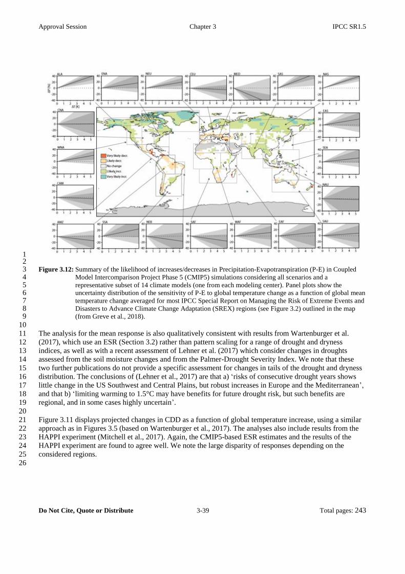
Approval Session Chapter 3 IPCC SR1.5
Do Not Cite, Quote or Distribute 3-39 Total pages: 243
1 2
Figure 3.12: Summary of the likelihood of increases/decreases in Precipitation-Evapotranspiration (P-E) in Coupled 3 Model Intercomparison Project Phase 5 (CMIP5) simulations considering all scenarios and a 4 representative subset of 14 climate models (one from each modeling center). Panel plots show the 5 uncertainty distribution of the sensitivity of P-E to global temperature change as a function of global mean 6 temperature change averaged for most IPCC Special Report on Managing the Risk of Extreme Events and 7 Disasters to Advance Climate Change Adaptation (SREX) regions (see Figure 3.2) outlined in the map 8 (from Greve et al., 2018). 9
10
The analysis for the mean response is also qualitatively consistent with results from Wartenburger et al. 11
(2017), which use an ESR (Section 3.2) rather than pattern scaling for a range of drought and dryness 12
indices, as well as with a recent assessment of Lehner et al. (2017) which consider changes in droughts 13
assessed from the soil moisture changes and from the Palmer-Drought Severity Index. We note that these 14
two further publications do not provide a specific assessment for changes in tails of the drought and dryness 15
distribution. The conclusions of (Lehner et al., 2017) are that a) ‘risks of consecutive drought years shows 16
little change in the US Southwest and Central Plains, but robust increases in Europe and the Mediterranean’, 17
and that b) ‘limiting warming to 1.5°C may have benefits for future drought risk, but such benefits are 18
regional, and in some cases highly uncertain’. 19
20
Figure 3.11 displays projected changes in CDD as a function of global temperature increase, using a similar 21
approach as in Figures 3.5 (based on Wartenburger et al., 2017). The analyses also include results from the 22
HAPPI experiment (Mitchell et al., 2017). Again, the CMIP5-based ESR estimates and the results of the 23
HAPPI experiment are found to agree well. We note the large disparity of responses depending on the 24
considered regions. 25
26

Approval Session Chapter 3 IPCC SR1.5
Do Not Cite, Quote or Distribute 3-40 Total pages: 243
Similarly as for Figures 3.8 and 3.11, Figure 3.14 includes an objective identification of “hot spots” / key 1
risks in dryness indices subdivided by regions, based on (Wartenburger et al., 2017). This analysis reveals 2
the following hot spots of drying, i.e. with increases in CDD, and decreases in P-E, Soil Moisture Anomalies 3
(SMA), and SPI12, with at least one of the indices displaying stiatistically significant drying: the 4
Mediterranean region (MED ; including Southern Europe, northern Africa, and the Near-East), Northeastern 5
Brazil (NEB), and Southern Africa. 6
7
8 9 Figure 3.13: Projected changes in consecutive dry days (CDD) as function of global temperature warming for IPCC 10
Special Report on Managing the Risk of Extreme Events and Disasters to Advance Climate Change 11 Adaptation (SREX) regions, based on empirical scaling relationship applied to Coupled Model 12 Intercomparison Project Phase 5 (CMIP5) data together with projected changes from the HAPPI multi-13 model experiment (bar plots on regional analyses and central plot, respectively). Same data basis and 14 analysis approach as in Figure 3.5 (Supplemantary Material 3.SM.2 for more details). 15 16
17

Approval Session Chapter 3 IPCC SR1.5
Do Not Cite, Quote or Distribute 3-41 Total pages: 243
Figure 3.14: Similar as Figures 3.8 and 3.11 but for changes in dryness indices. Significance of differences of regional 1 drought and dryness indices between the 1.5°C and 2°C global mean temperature targets (rows). 2 Definition of indices: CDD: Consecutive Dry Days; P-E: Precipitation minus Evaporation; SMA: Soil 3 Moisture Anomalies; SPI12: 12-month SPI. Columns indicate regions and global land (see Figure 3.2 for 4 definitions). Significant differences are shown in light blue/brownshading (increases in indices indicated 5 with + sign, decreases indicated with – sign; the light blue shading indicates decreases in dryness 6 (decreases in CDD, or increases in P-E, SMA or SPI12) and the light brown shading indicates increases in 7 dryness (increases in CDD, or decreases in P-E, SMA or SPI12). Insignificant differences are shown in 8 grey shading. Same data basis and analaysis approach as in Figure 3.7 (see Supplemantary Material 9 3.SM.2 for more details). 10
11
Overall the available literature, consistent with this analysis, reports particularly strong increases in dryness 12
and decreases in water availability in Southern Europe and the Mediterranean when shifting from a 1.5°C to 13
a 2°C global warming (Schleussner et al., 2016b; Lehner et al., 2017; Wartenburger et al., 2017; Greve et al., 14
2018; Samaniego et al., 2018; Figure 3.13). The fact that this is a region that is also already displaying 15
substantial drying in the observational record (Seneviratne et al., 2012; Sheffield et al., 2012; Greve et al., 16
2014; Gudmundsson and Seneviratne, 2016; Gudmundsson et al., 2017) provides additional evidence 17
supporting this tendency, suggesting that it is a hot spot of dryness change above 1.5°C (see also Box 3.2). 18
The other identified hot spots, Southern Africa and Northeastern Brazil, are also consistently shown to 19
display drying trends in other publications for higher levels of forcing (e.g., Orlowsky and Seneviratne, 20
2013), although there are so far to our knowledge no studies reporting observed drying trends in these 21
regions. There are substantial increases in risk of dryness (medium confidence) in both the Mediterranean 22
region and South Africa at 2°C versus 1.5°C global warming, because these regions display significant 23
changes in two dryness indicators (CDD and SMA) at these two global warming levels (Figure 3.14). There 24
is low confidence elsewhere due to lack of consistency in analyses with different models or different dryness 25
indicators. However, in many regions, there is medium confidence that most extreme risks of changes in 26
dryness are avoided at 2°C versus 1.5°C (Figure 3.12). 27
28
In summary, in terms of drought and dryness, limiting global warming to 1.5ºC may substantially reduce the 29
probability of extreme changes in water availability in some regions compared to changes for 2°C global 30
warming (medium confidence). When shifting from 1.5 to 2°C, available studies and analyses suggest strong 31
increases in dryness and reduced water availability in the Mediterranean region (including Southern Europe, 32
northern Africa, and the Near-East) and in Southern Africa (medium confidence). Based on observations and 33
model experiments, a drying trend is already detectable in the Mediterranean region, i.e. for a global warming 34
of less than 1°C (medium confidence). 35
36
[START BOX 3.2 HERE] 37
Mediterranean Basin and the Middle East Droughts 38
39
Human society has developed in tandem with the natural environment of the Mediterranean Basin over 40
several millennia, laying the ground for diverse and culturally rich communities. Even if advances in 41
technology may offer some protection from climatic hazards, the consequences of climatic change for 42
inhabitants of the Mediterranean continue to depend on the long term interplay between an array of societal 43
and environmental factors (Holmgren et al., 2016). This makes this region an example of strong vulnerability 44
and various adaptation responses. Previous IPCC assessments and recent publications project regional 45
changes in climate under increased warming, including consistent climate model projections of increased 46
precipitation deficit amplified by strong regional warming (Seneviratne et al., 2012; Christensen et al., 2013; 47
Collins et al., 2013; Greve and Seneviratne, 2015; Section 3.3.3). 48

Approval Session Chapter 3 IPCC SR1.5
Do Not Cite, Quote or Distribute 3-42 Total pages: 243
1
A good example of such long history of resilience is the Eastern Mediterranean region, which has exhibited a 2
strong negative trend in precipitation since 1960 (Mathbout et al., 2017) and experienced an intense and 3
prolonged drought episode between 2007 and 2010 (Kelley et al., 2015). This drought was the longest and 4
the most intense in the last 900 years (Cook et al., 2016). Some authors (e.g., Trigo et al., 2010; Kelley et al., 5
2015) assert that very low precipitation levels have driven a steep decline in agricultural productivity in the 6
Euphrates and Tigris catchment basins, and displaced hundreds of thousands of people, mainly in Syria. 7
Impacts have also been noticed on the water resource (Yazdanpanah et al., 2016) and the crop performance 8
in Iran (Saeidi et al., 2017). Many historical periods of turmoil have coincided with severe droughts, for 9
example the drought which occurred at the end of the Bronze Age, approximately 3200 years ago 10
(Kaniewski et al., 2015). In this instance, a number of flourishing Eastern Mediterranean civilizations 11
collapsed, and rural settlements re-emerged with agro-pastoral activities and limited long-distance trade. This 12
illustrates how some vulnerable regions are forced to pursue drastic adaptive responses, including migration 13
and societal structure changes. 14
15
The potential evolution of drought conditions under 1.5°C/2°C warming (Section 3.3.4) can be analyzed by 16
comparing the 2008 drought (high temperature, low precipitation) with the 1960 drought (low temperature, 17
low precipitation) (Kelley et al., 2015). Though the precipitation deficits were comparable, the 2008 drought 18
was amplified by increased evapotranspiration induced by much higher temperatures (a mean increase of 19
1°C on the 1931-2008 period on Syria) and a large population increase (from 5 million in 1960 to 22 million 20
in 2008). Koutroulis et al. (2013) projects that of the 18% decrease of water availability for Crete under a 21
2°C global warming at the end of the 21st century, only 6% is due to decreased precipitation (the rest is due 22
to an increase in evapotranspiration). This study and others like it confirm an important risk of extreme 23
drought conditions for the Middle East (even higher in continental locations than in islands) with a 1.5°C 24
global warming (Jacob et al., 2018), consistent with current observed changes (Greve et al., 2014); Section 25
3.3.4). Risks of drying in the Mediterranean region can be substantially reduced if global warming is limited 26
to 1.5°C compared to 2°C or higher levels of warming (Guiot and Cramer, 2016); see also Section 3.4.3). 27
Higher warming levels may induce strong levels of vulnerability exacerbated by large changes in 28
demography. 29
[END BOX 3.2 HERE] 30
31
3.3.5 Runoff and fluvial flooding 32
33
Observed and attributed changes in runof and river flooding 34
There has been progress since the AR5 in identifying historical changes in streamflow and continental 35
runoff. Dai (2016) using available streamflow data shows that long‐term (1948–2012) flow trends are 36
statistically significant only for 27.5% of the 200 world’s major rivers with negative trends outnumbering the 37
positive ones. Although streamflow trends are mostly non-statistically significant, they are consistent with 38
observed regional precipitation changes. From 1950 to 2012, precipitation and runoff have increased over 39
southeastern South America, central and northern Australia, the central and northeast United States, central 40
and northern Europe, and most of Russia and decreased over most of Africa, East and South Asia, eastern 41
coastal Australia, southeastern and northwestern United States, western and eastern Canada, the 42
Mediterranean region and in some regions of Brazil (Dai, 2016). 43
44
A large part of the observed regional trends in streamflow and runoff could have resulted from internal 45
multidecadal and multiyear climate variations, especially the Pacific Decadal Variability (PDV), the Atlantic 46
Multidecadal Oscillation (AMO) and the El Niño-Southern Oscillation (ENSO) although the effect of 47

Approval Session Chapter 3 IPCC SR1.5
Do Not Cite, Quote or Distribute 3-43 Total pages: 243
anthropogenic greenhouse gasses and aerosols could also be important (Hidalgo et al., 2009; Gu and Adler, 1
2013, 2015; Chiew et al., 2014; Luo et al., 2016; Gudmundsson et al., 2017). Additionally, other human 2
activities can influence the hydrological cycle such as land-use/land-cover change, modifications in river 3
morphology and water table depth, construction and operation of hydropower plants, dikes and weirs, 4
wetland drainage and agricultural practices such as water withdrawal for irrigation. All of these can also 5
have a large impact on runoff at river basin scales although there is less agreement over their influence on 6
global mean runoff (Gerten et al., 2008; Sterling et al., 2012; Hall et al., 2014; Betts et al., 2015; Arheimer et 7
al., 2017). Some studies suggest that increases in global runoff resulting from changes in land-cover or land-8
use (predominantly deforestation) are counterbalanced by decreases from irrigation (Gerten et al., 2008; 9
Sterling et al., 2012). Likewise, forest and grassland fires can also modify the hydrological response at a 10
watershed scale when the burned area is significant (Versini et al., 2013; Springer et al., 2015; Wine and 11
Cadol, 2016). 12
13
Few studies explore observed changes in extreme streamflow and river flooding since the IPCC AR5. 14
Mallakpour and Villarini (2015) analyzed changes of flood magnitude and frequency in Central United 15
States considering stream gauge daily records with at least 50 years of data ending no earlier than 2011. 16
They showed that flood frequency has increased while there was limited evidence of a decrease in flood 17
magnitude in this region. Stevens et al. (2016) found a rise in the number of reported floods in the United 18
Kingdom during the period 1884-2013 with flood events appearing more frequently towards the end of the 19
20th century. A peak was identified in 2012 when annual rainfall was the second highest in over 100 years. 20
Do et al. (2017) computed the trends in annual maximum daily streamflow data across the globe over the 21
1966–2005 period. They found decreasing trends for a large number of stations in western North America 22
and Australia, and increasing trends in parts of Europe, eastern North America, parts of South America and 23
southern Africa. 24
25
In summary, streamflow trends since 1950 are non-statistically significant in most of the world’s largest 26
rivers (high confidence), while flood frequency and extreme streamflow increased in some regions (high 27
confidence). 28
29
Projected changes at 1.5°C versus 2°C in runoff and river flooding 30
Global-scale assessments of projected changes on freshwatr systems generally suggest that areas with either 31
positive or negative changes in mean annual streamflow are smaller for 1.5C than for 2C global warming 32
(Betts et al., 2018; Döll et al., 2018). Döll et al. (2018) found that only 11% of the global land area 33
(excluding Greenland and Antarctica) shows statistically significant larger hazard at 2C than at 1.5C. 34
Significant decreases are found for 13% of the global land area for both global warming levels, while 35
significant increases are projected to occur for 21% of the global land area for 1.5C, and rise to between 36
26% (Döll et al., 2018) and approximately 50% (Betts et al., 2018) for 2C. 37
38
At the regional scale, projected runoff changes in general follow the spatial extent of projected changes in 39
precipitation (see Section 3.3.3). Emerging literature shows runoff projections for different warming levels. 40
For 2C global warming, an increase in runoff is projected for much of the high northern latitudes, Southeast 41
Asia, East Africa, north-eastern Europe, India, and parts of, Austria, China, Hungary, Norway, Sweden, the 42
northwest Balkans, and Sahel (Schleussner et al., 2016b; Donnelly et al., 2017; Zhai et al., 2017; Döll et al., 43
2018). Addtionally, decreases are projected in the Mediterranean region, South Australia, Central America 44
and Central and Southern South America (Schleussner et al., 2016b; Donnelly et al., 2017; Döll et al., 2018). 45
Differences between 1.5C and 2C would be most prominent in the Mediterranean where the median 46

Approval Session Chapter 3 IPCC SR1.5
Do Not Cite, Quote or Distribute 3-44 Total pages: 243
reduction in annual runoff is expected to be about 9% (likely range 4.5–15.5%) at 1.5C, while at 2C 1
warming, runoff could decrease by 17% (likely range 8–25%) (Schleussner et al., 2016b). Consistently, Döll 2
et al. (2018) found that for an increase in global warming from 1.5°C to 2°C, statistically insignificant 3
changes of the mean annual streamflow around the Mediterranean region become significant with decreases 4
of 10–30%. Donnelly et al. (2017) found an intense decrease in runoff along both the Iberian and Balkan 5
coasts as warming level increases. 6
7
Basin-scale projections of river runoff at different warming levels are available for many regions. Betts et al. 8
(2018) assessed runoff changes in 21 of the world major river basins at 1.5C and 2C global warming 9
(Figure 3.15). They found a general tendency towards increased runoff in the majority of the basins except in 10
the Amazon, Orange, Danube and Guadiana basins where the range of projections indicate decreased mean 11
flows (Figure 3.13). In the case of the Amazon, mean flows are projected to decline by up to 25% for 2°C 12
global warming. Gosling et al. (2017) analyzed the impact of global warming of 1°C, 2°C and 3°C above 13
pre-industrial levels on river runoff at catchment scale, focusing on eight major rivers in different continents: 14
Upper Amazon, Darling, Ganges, Lena, Upper Mississippi, Upper Niger, Rhine and Tagus. Their results 15
show that the sign and magnitude of change with global warming for the Upper Amazon, Darling, Ganges, 16
Upper Niger and Upper Mississippi is unclear, while the Rhine and Tagus may experience decreases in 17
projected runoff and the Lena may increase. Donnelly et al. (2017) analyzed the mean flow response to 18
different warming levels for six major European rivers: Glomma, Wisla, Lule, Ebro, Rhine and Danube. 19
Consistent with the increases in mean runoff in large parts of northern Europe, the Glomma, Wisla and Lule 20
rivers could increase their discharges with global warming while the Ebro could decrease in part due to a 21
decrease in runoff in southern Europe. In the case of the Rhine and Danube rivers, Donnelly et al. (2017) did 22
not find clear results. Projected mean annual runoff of the Yiluo River catchment in northern China will 23
decrease by 22% for 1.5°C and by 21% for 2°C, while the the mean annual runoff for the Beijiang River in 24
southern China, is projected to increase by less than 1% and 3% in comparicon to the studied baseline period 25
for 1.5°C and 2°C respectively (L. Liu et al., 2017). Chen et al. (2017) assessed the future changes of water 26
resources in the Upper Yangtze River basin for the same warming levels and found a slight decrease in the 27
annual discharge for 1.5°C which reverses sign for 2°C. Montroull et al. (2018) studied the hydrological 28
impacts of the main rivers (Paraguay, Paraná, Iguazú and Uruguay) in La Plata basin in South America under 29
1.5°C and 2°C global warming and for two emission scenarios. The Uruguay basin shows increases in 30
streamflow in all scenarios/warming targets except for the combination of RCP8.5/1.5C warming. The 31
increase is approximately 15% above the 1981–2000 reference period for 2C global warming and the 32
RCP4.5 scenario. For the other three rivers the sign of the change in mean streamflow highly depends on the 33
RCP and GCM used. 34
35
Marx et al. (2018) analyzed how hydrological low flows in Europe are affected under different global 36
warming levels (1.5C, 2C and 3C). The Alpine region shows the strongest low flow increase from 22% 37
for 1.5C to 30% for 2C because of the snow melt contribution, while in the Mediterranean low flows are 38
expected to decrease due to the projected decreases in annual precipitation. Döll et al. (2018) found that 39
extreme low flows in the tropical Amazon, Congo and Indonesian basins could decrease by 10% while in the 40
southwestern part of Russia they could increase by 30% at 1.5C. For 2C, projected increases of extreme 41
low flows are exacerbated in the higher northern latitudes and in eastern Africa, India and Southeast Asia 42
while projected decreases intensify in the Amazon basin, Western United States, central Canada, and in 43
Southern and Western Europe, although not in the Congo basin or Indonesia, where models show less 44
agreement. 45
46

Approval Session Chapter 3 IPCC SR1.5
Do Not Cite, Quote or Distribute 3-45 Total pages: 243
1 Figure 3.15: Runoff changes in twenty-one of the world major river basins at 1.5C (blue) and 2C (orange) global 2
warming simulated by the Joint UK Land Environment Simulator (JULES) ecosystem–hydrology model 3 under the ensemble of six climate projections. Boxes show the 25th and 75th percentile changes, whiskers 4 show the range, circles show the four projections that do not define the ends of the range, and crosses 5 show the ensemble means. Numbers in square brackets show the ensemble-mean flow in the baseline 6 (millimetres of rain equivalent) (from Betts et al., 2018). 7
8
Recent analysis of projections in river flooding and extreme runoff and flows are available for different 9
global warming levels. At the global scale, Alfieri et al. (2017) assessed the frequency and magnitude of 10
river floods and their impacts under 1.5C, 2C, and 4C global warming scenarios. They found that flood 11
events with occurrence interval larger than the return period of present flood protections are projected to 12
increase in all continents under all considered warming levels, leading to widespread increment in the flood 13
hazard. Döll et al. (2018) found that high flows are projected to increase significantly on 11% and 21% of 14
the global land area at 1.5C and 2C respectively. Significantly increased high flows are expected to occur 15
in South and Southeast Asia and Central Africa at 1.5C which intensify under 2C and include parts of 16
South America. 17
18
At continental scale, Donnelly et al. (2017) and Thober et al. (2018) explored climate change impacts on 19
European high flows and/or floods under 1.5C, 2C, and 3C global warming. Thober et al. (2018) 20

Approval Session Chapter 3 IPCC SR1.5
Do Not Cite, Quote or Distribute 3-46 Total pages: 243
identified the Mediterranean region as a hotspot of change with significant decreases of −11% (-13%) in high 1
flows at 1.5°C (2C) mainly resulting from reduced precipitation (Box 3.2). In Northern regions, high flows 2
are projected to rise between 1%-5% for 1.5C and 2C respectively due to increasing precipitation, although 3
floods could decrease by 6% in both scenarios due to less snowmelt. Donnelly et al. (2017) found that high 4
runoff levels could rise in intensity, robustness and spatial extent over large parts of continental Europe, with 5
increasing warming level. For 2C, flood magnitudes are expected to increase significantly in Europe south 6
of 60N, except for some regions (Bulgaria, Poland, southern Spain) while they are projected to decrease in 7
most of Finland, northwestern Russia and northern Sweden, with the exception of southern Sweden and 8
some coastal areas in Norway where floods may increase (Roudier et al., 2016). At basin scale, Mohammed 9
et al. (2017) found that floods are projected to be more frequent and flood magnitudes greater at 2°C than at 10
1.5°C in the Brahmaputra River in Bangladesh. 11
12
In coastal regions, increases in heavy precipitation associated with tropical cyclones (Section 3.3.6) combined 13
with increased sea levels (Section 3.3.9) may lead to increased flooding (Section 3.4.5). 14
15
In summary, there is medium confidence that a global warming of 2°C would lead to an expansion of the area 16
with significant increases in runoff as well as of the area affected by flood hazard compared to conditions at 17
1.5°C global warming. A global warming of 1.5°C would also lead to an expansion of the global land area 18
with significant increases in runoff (medium confidence) as well as to an increase in flood hazard in some 19
regions (medium confidence) compared to present day conditions. 20
21
22
3.3.6 Tropical cyclones and extratropical storms 23
24
Most recent studies on observed trends in the attributes of tropical cyclones are focusing on the satellite era 25
starting in 1979 (Rienecker et al., 2011), but the study of observed trends is complicated by the heterogeneity 26
of constantly advancing remote sensing techniques and instrumentation during this period (e.g., Landsea et 27
al., 2006; Walsh et al., 2016). Numerous studies towards and beyond AR5 have reported a decreasing trend 28
in the global number of tropical cyclones and/or the globally accumulated cyclonic energy (Emanuel, 2005; 29
Elsner et al., 2008; Knutson et al., 2010; Holland and Bruyère, 2014; Klotzbach and Landsea, 2015; Walsh et 30
al., 2016). A theoretical physical basis for such a decrease to occur under global warming has recently been 31
provided by Kang and Elsner (2015). However Klotzbach (2006), using a relatively short (twenty year) 32
relatively homogeneous remotely sensed record reported no significant trends in global cyclonic activity, 33
consistent with more recent findings of Holland and Bruyère (2014). Such contradictions, in combination 34
with the fact that the almost four-decade long period of remotely sensed observations remains relatively 35
short to distinguish anthropogenically induced trends from decadal and multi-decadal variability, implies that 36
there is only low confidence regarding changes in global tropical cyclone numbers under global warming 37
over the last four decades. 38
39
Studies on the detection of trends in the occurrence of very intense tropical cyclones (category 4 and 5 40
hurricanes on the Saffir-Simpson scale) over recent decades have yielded contradicting results. Most studies 41
have reported increases in these systems (Emanuel, 2005; Webster et al., 2005; Klotzbach, 2006; Elsner et 42
al., 2008; Knutson et al., 2010; Holland and Bruyère, 2014; Walsh et al., 2016), and in particular for the 43
North Atlantic, North Indian and South Indian Ocean basins (e.g., Singh et al., 2000; Singh, 2010; Kossin et 44
al., 2013; Holland and Bruyère, 2014; Walsh et al., 2016). In the North Indian Ocean over the Arabian Sea, 45
an increase in the frequency of extremely severe cyclonic storms has been reported and attributed to 46
anthropogenic warming (Murakami et al., 2017). However, to the east over the Bay of Bengal, tropical 47

Approval Session Chapter 3 IPCC SR1.5
Do Not Cite, Quote or Distribute 3-47 Total pages: 243
cyclones and severe tropical cyclones have exhibited decreasing trends over the period 1961-2010, although 1
the ratio between severe tropical cyclones and cyclones is increasing (Mohapatra et al., 2017). Moreover, 2
studies that have used more homogeneous records but that were consequently limited to rather short periods 3
of 20 to 25 years in length, have reported no statistically significant trends or decreases in the global number 4
of these systems (Kamahori et al., 2006; Klotzbach and Landsea, 2015). CMIP5 model simulations of the 5
historical period have also not produced anthropogenically induced trends in very intense tropical cyclones 6
(Bender et al., 2010; Knutson et al., 2010, 2013; Camargo, 2013; Christensen et al., 2013), consistent with 7
the findings of Klotzbach and Landsea (2015). There is consequently low confidence in the larger number of 8
studies reporting increasing trends in the global number of very intense cyclones. 9
10
GCM projections of the changing attributes of tropical cyclones under high levels of greenhouse gas forcing 11
(3°C to 4°C) are consistently indicating decreases in the global number of tropical cyclones (Knutson et al., 12
2010, 2015; Sugi and Yoshimura, 2012; Christensen et al., 2013; Yoshida et al., 2017). A smaller number of 13
studies based on statistical downscaling methodologies are contradicting these findings, however, and are 14
indicative of increases in the global number of tropical cyclones under climate change (Emanuel, 2017). 15
Most studies also indicate increases in the global number of very intense tropical cyclones under high levels 16
of global warming (Knutson et al., 2015; Sugi et al., 2017) consistent with dynamic theory (Kang and Elsner, 17
2015), although a few studies contradict this finding (e.g., Yoshida et al., 2017). Hence, we assess that under 18
3 to 4 °C of warming it is more likely than not (medium confidence) that the global number of tropical 19
cyclones would decrease whilst the number of very intense cyclones would increase. 20
21
Only two studies have to date directly explored the changing tropical cyclone attributes under 1.5°C versus 22
2°C of global warming. Using a high resolution global atmospheric model, Wehner et al. (2017) concluded 23
that the differences in tropical cyclone statistics under 1.5°C versus 2°C stabilization scenarios as defined by 24
the HAPPI protocols (Mitchell et al., 2017) are small. Consistent with the majority of studies performed for 25
higher degrees of global warming, the total number of tropical cyclones is projected to decrease under global 26
warming, whilst the most intense (category 4 and 5) cyclones are projected to occur more frequently. These 27
very intense storms are projected to be associated with higher peak wind speeds and lower central pressures 28
under 2°C versus 1.5°C of global warming. The accumulated cyclonic energy is projected to decrease 29
globally from 1.5 to 2 °C, in association with a decrease in the global number of tropical cyclones under 30
progressively higher levels of global warming. It is also noted that heavy rainfall associated with tropical 31
cyclones has been assessed in the IPCC SREX to likely increase under increasing global warming 32
(Seneviratne et al., 2012). Two recent articles suggest that there is high confidence that global warming for 33
present conditions (i.e. about 1°C of global warming, see Section 3.3.1) has increased the heavy precipitation 34
associated with the 2017 Hurricane Harvey by about 15% or more (Risser and Wehner, 2017; van 35
Oldenborgh et al., 2017). Hence, it can be inferred, under the assumption of linear dynamics, that further 36
increases in heavy precipitation would occur under 1.5°C, 2°C and higher levels of global warming (medium 37
confidence). Using a high resolution regional climate model, (Muthige et al., 2018) also explored the effects 38
of different degrees of global warming on tropical cyclones over the southwest Indian Ocean, in transient 39
simulations that downscaled a number of RCP8.5 GCM projections. Decreases in tropical cyclone 40
frequencies are projected under both 1.5ºC and 2°C of global warming. The decreases in cyclone frequencies 41
under 2°C global warming are somewhat larger than under 1.5°C of global warming, but with no further 42
decreases projected under 3°C of global warming. This suggests that 2°C of warming, at least in these 43
downscaling simulations, represent a type of stabilization level in terms of tropical cyclone formation over 44
the southwest Indian Ocean and landfall over southern Africa (Muthige et al., 2018). There is thus limited 45
evidence that the global number of tropical cyclones will be less under 2°C of global warming compared to 46
1.5 °C of warming, but with an increase in the number of very intense cyclones (low confidence). 47

Approval Session Chapter 3 IPCC SR1.5
Do Not Cite, Quote or Distribute 3-48 Total pages: 243
1
The global response of the mid-latitude atmospheric circulation to 1.5 and 2°C of warming was investigated 2
using the HAPPI ensemble with a focus on the winter season (Li et al., 2018). Under 1.5 °C of global 3
warming a weakening of storm activity over North America, an equatorward shift of the North Pacific jet 4
exit and an equatorward intensification of the South Pacific jet are projected. Under an additional 0.5°C of 5
warming a poleward shift of the North Atlantic jet exit and an intensification on the flanks of the Southern 6
Hemisphere storm track become more pronounced. The weakening of the Mediterranean storm track that is 7
projected under low mitigation emerges in the 2 °C warmer world (Li et al., 2018). The AR5 (Stocker et al., 8
2013) assessed that under high greenhouse forcing (3°C or 4°C) there is low confidence in projections of 9
poleward shifts of the North-Hemisphere storm tracks, while there is high confidence that there would be a 10
small poleward shift of the South-Hemisphere storm tracks.In the context of this report, we assess that there 11
is limited evidence and low confidence in whether any projected signal for higher levels of warming is to be 12
well-manifested under 2°C of global warming. 13
14
15
3.3.7 Ocean circulation and temperature 16
17
It is virtually certain that the temperature of the upper layers of the ocean (0–700 m) has been increasing at a 18
rate just behind that of the warming trend for the planet. The surface of three ocean basins have warmed over 19
the period 1950–2016 (by 0.11°C, 0.07°C, and 0.05°C per decade for the Indian, Atlantic and Pacific oceans 20
respectively; Hoegh-Guldberg et al., 2014, AR5 Chapter 30), with the greatest changes occurring at the 21
highest latitudes. Isotherms (i.e. lines of equal temperature) of sea surface temperature (SST) are traveling to 22
higher latitudes at rates of up to 40 km per year (Burrows et al., 2014; García Molinos et al., 2015). Long-23
term patterns of variability make detecting signals due to climate change complex, although the recent 24
acceleration of changes to the temperature of the surface layers of the ocean has made the climate signal 25
more distinct (Hoegh-Guldberg et al., 2014). There is also evidence of significant increases in the frequency 26
of marine heatwaves in the observational record (Oliver et al., 2018), consistent with changes in mean ocean 27
temperatures (high confidence). Increasing climate extremes in the ocean are associated with the general rise 28
in global average surface temperature as well as more intense patterns of climate variability (e.g., climate 29
change intensification of ENSO). Increased heat in the upper layers of the ocean is also driving more intense 30
storms and greater rates of inundation, which, together with sea level rise, are already driving significant 31
impacts to sensitive coastal and low-lying areas. 32
33
Increasing land-sea temperature gradients, as induced by higher rates of continental warming compared to 34
the surrounding oceans under climate change, have the potential to strengthen upwelling systems associated 35
with the eastern boundary currents (Benguela, Canary, Humboldt and Californian Currents) (Bakun, 1990). 36
Observed trends support the conclusion that a general strengthening of longshore winds has occurred 37
(Sydeman et al., 2014), but are unclear in terms of trends detected in the upwelling currents themselves 38
(Lluch-Cota et al., 2014). Projecting the scale of the changes between 1oC and 1.5oC, and 1.5oC and 2oC is 39
only informed by the changes over the past change in GMST of 0.5oC (low confidence). However, the weight 40
of evidence from GCM projections of future climate change indicates the general strengthening of the 41
Benguela, Canary and Humboldt upwelling systems under enhanced anthropogenic forcing (D. Wang et al., 42
2015) is likely to occur. This strengthening is projected to be stronger at higher latitudes. In fact, evidence 43
from regional climate modelling is supportive of an increase in long-shore winds at higher latitudes, but at 44
lower latitudes long-shore winds may decrease as a consequence of the poleward displacement of the 45
subtropical highs under climate change (Christensen et al., 2007; Engelbrecht et al., 2009). 46
47
Approval Session Chapter 3 IPCC SR1.5
Do Not Cite, Quote or Distribute 3-49 Total pages: 243
It is more likely than not that the Atlantic Meridional Overturning Circulation (AMOC) has been weakening 1
in recent decades, given the detection of the cooling of surface waters in the north Atlantic and evidence that 2
the Gulf Stream has slowed by 30% since the late 1950s (Srokosz and Bryden, 2015; Caesar et al., 2018). 3
There is only limited evidence linking the current anomalously week state of AMOC to anthropogenic 4
warming (Caesar et al., 2018). It is very likely that the AMOC will weaken over the 21st century. Best 5
estimates and range for the reduction from CMIP5 are 11% (1 to 24%) in RCP2.6 and 34% (12 to 54%) in 6
RCP8.5 (AR5). There is no evidence indicating significantly different amplitudes of AMOC weakening for 7
1.5°C versus 2°C of global warming. 8
9
10
3.3.8 Sea ice 11
12
Summer sea ice in the Arctic has been retreating rapidly in recent decades. During the period 1997 to 2014 13
for example, the monthly mean sea-ice extent during September decreased on average by 130,000 km² per 14
year (Serreze and Stroeve, 2015). This is about four times as fast as the September sea-ice loss during the 15
period 1979 to 1996. Also sea-ice thickness has decreased substantially, with an estimated decrease in ice 16
thickness of more than 50% in the central Arctic (Lindsay and Schweiger, 2015). Sea-ice coverage and 17
thickness also decrease in CMIP5-model simulations of the recent past, and are projected to decrease in the 18
future (Collins et al., 2013). However, the modeled sea-ice loss in most CMIP5 models is much weaker 19
than observed. Compared to observations, the simulations are weak in terms of their sensitivity to both 20
global mean temperature rise (Rosenblum and Eisenman, 2017) and to anthropogenic CO2 emissions (Notz 21
and Stroeve, 2016). This mismatch between the observed and modeled sensitivity of Arctic sea ice implies 22
that the multi-model-mean response of future sea-ice evolution probably underestimates the sea-ice loss for 23
a given amount of global warming. To address this issue, studies estimating the future evolution of Arctic 24
sea ice tend to bias correct the model simulations based on the observed evolution of Arctic sea ice in 25
response to global warming. Often based on such bias correction, pre-AR5 and post-AR5 studies agree that 26
for 1.5 °C global warming relative to pre-industrial levels, the Arctic Ocean will maintain a sea-ice cover 27
throughout summer for most years (Collins et al., 2013; Notz and Stroeve, 2016; Screen and Williamson, 28
2017; Jahn, 2018; Niederdrenk and Notz, 2018; Sigmond et al., 2018). For 2°C global warming relative to 29
pre-industrial levels, chances of an ice-free Arctic during summer are substantially higher (Screen and 30
Williamson, 2017; Jahn, 2018; Niederdrenk and Notz, 2018; Screen et al., 2018; Sigmond et al., 2018). The 31
Arctic is very likely to have experienced at least one ice-free Arctic summer after about 10 years of 32
stabilized warming at 2°C compared to after about 100 years of stabilized warming at 1.5°C (Jahn, 2018; 33
Screen et al., 2018; Sigmond et al., 2018). For a specific given year under stabilized warming of 2°C, 34
studies based on large ensembles of simulations with a single model estimate the likelihood for ice-free 35
conditions as 35% without a bias correction of the underlying model (Sanderson et al., 2017; Jahn, 2018); 36
as between 10% and >99% depending on the observational record used to correct the sensitivity of sea ice 37
decline to global warming in the underlying model (Niederdrenk and Notz, 2018); and as 19% based on a 38
procedure to correct for biases in the climatological sea ice coverage in the underlying model (Sigmond et 39
al., 2018). The uncertainty of the first year of the occurrence of an ice-free Arctic Ocean arising from 40
internal variability is estimated to be about 20 years (Notz, 2015; Jahn et al., 2016). 41
42
The more recent estimates of the warming necessary to achieve an ice-free Arctic Ocean during summer are 43
lower than the ones given in AR5 (about 2.6C-3.1C relative to preindustrial or 1.6C-2.1C global 44
warming relative to the present day), which was similar to the estimate of 3C relative to preindustrial 45
levels (or 2C global warming relative to the present day) by Mahlstein and Knutti (2012) based on bias-46
corrected CMIP3 models. Rosenblum and Eisenman (2016) explain why the sensitivity estimated by 47

Approval Session Chapter 3 IPCC SR1.5
Do Not Cite, Quote or Distribute 3-50 Total pages: 243
Mahlstein and Knutti (2012) might be too low, estimating instead that September sea ice in the Arctic 1
disappears for 2°C relative to preindustrial (or about 1°C global warming relative to the present day), in line 2
with the other recent estimates. Notz and Stroeve (2016) use the observed correlation between September 3
sea-ice extent and cumulative CO2 emissions to estimate that the Arctic Ocean would become nearly sea-4
ice-free during September with a further 1000 Gt of emissions, which also implies a sea-ice loss at about 5
2°C global warming. Some of the uncertainty in these numbers derives from the possible impact of aerosols 6
(Gagne et al., 2017) and of volcanic forcing (Rosenblum and Eisenman, 2016). During winter, little Arctic 7
sea ice is projected to be lost for either 1.5°C or 2ºC global warming (Niederdrenk and Notz, 2018). 8
9
Regarding the behavior of Arctic sea ice under decreasing temperatures following a possible overshoot of a 10
long-term temperature target, a substantial number of pre-AR5 studies have found that there is no indication 11
of hysteresis behavior of Arctic sea ice (Holland et al., 2006; Schroeder and Connolley, 2007; Armour et 12
al., 2011; Sedláček et al., 2011; Tietsche et al., 2011; Boucher et al., 2012; Ridley et al., 2012). In 13
particular, the relationship between Arctic sea-ice coverage and GMST is found to be indistinguishable 14
between a warming scenario and a cooling scenario. These results have been confirmed by post-AR5 15
studies (Li et al., 2013; Jahn, 2018), which implies high confidence that an intermediate temperature 16
overshoot has no long-term consequences for Arctic sea-ice coverage. 17
18
In the Antarctic, sea ice shows regionally contrasting trends, with for example strongly decreased sea-ice 19
coverage near the Antarctic peninsula and increased sea-ice coverage in the Amundsen Sea (Hobbs et al., 20
2016). Averaged over these contrasting regional trends, there has been a slow long-term increase in overall 21
sea-ice coverage in the Southern Ocean, with, however, comparably low ice coverage from September 2016 22
onwards. Collins et al. (2013) have low confidence in Antarctic sea ice projections because of the wide 23
range of model projections and an inability of almost all models to reproduce observations such as the 24
seasonal cycle, interannual variability and the long-term slow increase. No studies are hence available to 25
robustly assess the possible future evolution of Antarctic sea ice under low-warming scenarios. 26
27
In summary, the probability of a sea-ice-free Arctic Ocean during summer is substantially higher at 2°C 28
compared to 1.5°C global warming relative to pre-industrial levels and it is very likely that there will be the 29
least one sea-ice-free Arctic summer after about 10 years of stabilized warming at 2°C, while about 100 30
years are required at 1.5°C. There is high confidence that an intermediate temperature overshoot has no 31
long-term consequences for Arctic sea-ice coverage. 32
33
34
3.3.9 Sea level 35
36
Sea level varies over a wide range of temporal and spatial scales, which can be divided into three broad 37
categories. These are Global Mean Sea Level (GMSL), regional variation about this mean, and the 38
occurrence of sea-level extremes associated with storm surges and tides. GMSL has been rising since the 39
late 19th century from the low rates of change that characterized the previous two millennia (Church et al., 40
2013). Slowing in the reported rate over the last two decades (Cazenave et al., 2014) may be attributable to 41
instrumental drift in the observing satellite system (Watson et al., 2015) and volcanoes (Fasullo et al., 42
2016). Accounting for the former results in rates (1993 to mid-2014) of between 2.6 and 2.9 mm yr-1 43
(Watson et al., 2015). The relative contributions from thermal expansion, glacier and ice-sheet mass loss, as 44
well as freshwater storage on land, are relatively well understood (Church et al., 2013; Watson et al., 2015) 45
and there attribution is dominated by anthropogenic forcing since 1970 (15±55% before 1950, 69±31% 46
after 1970) (Slangen et al., 2016). 47
Approval Session Chapter 3 IPCC SR1.5
Do Not Cite, Quote or Distribute 3-51 Total pages: 243
1
There has been a significant advance in the literature since AR5, which has seen the development of Semi-2
Empirical Models (SEMs) into a broader emulation-based approach (Kopp et al., 2014; Mengel et al., 2016; 3
Nauels et al., 2017) that is partially based on the results from more detailed, process-based modelling, 4
where available. Church et al. (2013) assigned low confidence to SEMs because of their assumption that the 5
relation between climate forcing and GMSL is the same in the past (calibration) and future (projection). 6
Probable future changes in the relative contributions of thermal expansion, glaciers and (in particular) ice 7
sheets invalidate this assumption, however recent emulation-based studies overcome this by considering 8
individual GMSL contributors separately and are therefore employed in this assessment. In this subsection, 9
the process-based literature of individual contributors to GMSL is considered for scenarios close to 1.5ºC 10
and 2ºC before assessing emulation-based approaches. 11
12
A limited number of processes-based studies are relevant to GMSL in 1.5ºC and 2ºC worlds. Marzeion et al. 13
(2018) force a global glacier model with temperature-scaled scenarios based on RCP2.6 to investigate the 14
difference between 1.5ºC and 2ºC and find little difference between scenarios in the glacier contribution to 15
GMSL at 2100 (54-97 mm relative to present day for 1.5ºC, and 63-112 mm for 2ºC using a 90% confidence 16
interval). This arises because melt during the remainder of the century is dominated by the response to 17
warming from preindustrial to present-day levels (in turn a reflection of the slow response times of glaciers). 18
Fuerst et al. (2015) make projections of Greenland ice sheet’s contribution to GMSL using an ice-flow 19
model forced by the regional climate model Modèle Atmosphérique Régional (MAR, considered by Church 20
et al., 2013) to be the ‘most realistic’ such model). They obtain an RCP2.6 range of 24-60 mm (1 standard 21
deviation) by the end of the century (relative to 2000 and consistent with the assessment of Church et al. 22
(2013)), however their projections do not allow the difference between 1.5ºC and 2ºC worlds to be evaluated. 23
24
The Antarctic ice sheet can contribute both positively and negatively to future GMSL rise by, respectively, 25
increases in outflow (solid ice lost directly to the ocean) and increases in snowfall (due to the increased 26
moisture-bearing capacity of a warmer atmosphere). Frieler et al. (2015) suggest a range of 3.5-8.7 % K-1 27
for this effect, which is consistent with the AR5. Observations from the Amundsen Sea sector of Antarctic 28
suggest an increase in outflow (Mouginot et al., 2014) over recent decades associated with grounding line 29
retreat (Rignot et al., 2014) and the influx of relatively warm Circumpolar Deepwater (Jacobs et al., 2011). 30
Literature on the attribution of these change to anthropogenic forcing is still in its infancy (Goddard et al., 31
2017; Turner et al., 2017a). RCP2.6-based projections of Antarctic outflow (Levermann et al., 2014; 32
Golledge et al., 2015; DeConto and Pollard, 2016, who include snowfall changes) are consistent with the 33
AR5 assessment of Church et al. (2013) for end-of-century GMSL for RCP2.6, and do not support 34
substantial additional GMSL rise by Marine Ice Sheet Instability or associated instabilities (see Section 35
3.6). While agreement is relatively good, concerns about the numerical fidelity of these models still exist 36
and this may affect the quality of their projections (Drouet et al., 2013; Durand and Pattyn, 2015). An 37
assessment of Antarctic contributions beyond the end of the century, in particular related to the Marine Ice 38
Sheet Instability, can be found in Section 3.6. 39
40
While some literature on process-based projections of GMSL at 2100 is available, it is insufficient to 41
distinguish between emission scenarios associated with 1.5ºC and 2ºC worlds. This literature is, however, 42
consistent with Church et al. (2013) assessment of a likely range of 0.28-0.61 m at 2100 (relative to 1986-43
2005) suggesting that AR5 assessment is still appropriate. Recent emulation-based studies show 44
convergence towards this AR5 assessment (Table 3.1) and offer the advantage of allowing a comparison 45
between 1.5ºC and 2ºC worlds. Table 3.1 presents a compilation of both recent emulation-based and SEM 46
studies. 47

Approval Session Chapter 3 IPCC SR1.5
Do Not Cite, Quote or Distribute 3-52 Total pages: 243
1 Table 3.1: Compilation of recent projections for sea level at 2100 (in cm) for Representative Concentration Pathway 2
(RCP)2.6, and 1.5 and 2.0 C scenarios. Upper and lower limits are shown for the 17-84% and 5-95% 3 confidence intervals quoted in the original papers. 4
Study Baseline RCP2.6 1.5ºC 2ºC
67% 90% 67% 90% 67% 90%
AR5 1986-2005 28-61
Kopp et al. (2014) 2000 37-65 29-82
Jevrejeva et al. (2016) 1986-2005 29-58
Kopp et al. (2016) 2000 28-51 24-61
Mengel et al. (2016) 1986-2005 28-56
Nauels et al. (2017) 1986-2005 35-56
Goodwin et al. (2017) 1986-2005 31-59
45-70
45-72
Schaeffer et al. (2012) 2000 52-96 54-99 56-105
Schleussner et al. (2016b) 2000 26-53 36-65
Bittermann et al. (2017) 2000 29-46 39-61
Jackson et al. (2018) 1986-2005 30-58
40-77
20-67
28-93
35-64
47-93
24-74
32-117
Sanderson et al. (2017) 50-80 60-90
Nicholls et al. (2018) 1986-2005 24-54 31-65
Rasmussen et al. (2018) 2000 35-64 28-82 39-76 28-96
Goodwin et al. (2018) 1986-2005 26-62 30-69
5
There is little consensus between the reported ranges of GMSL rise (Table 3.1), in particular at their upper 6
limit, however there is medium agreement that GMSL at 2100 would be 0-0.2 m higher in a 2ºC world 7
compared to 1.5 ºC with a most likely value of 0.1 m. There is medium confidence in this assessment 8
because of issues associated with both projections of the Antarctic contribution to GMSL that are employed 9
in emulation-based studies (see above) and the issues previously identified with SEMs (Church et al., 10
2013). 11
12
Translating projections of GMSL to the scale of coastlines and islands requires two further steps. The first 13
accounts for regional changes associated with changing water and ice loads (such as Earth’s gravitational 14
field and rotation, and vertical land movement), as well as accounting for spatial differences in ocean heat 15
uptake and circulation. The second maps regional sea level on to changes in the return periods of particular 16
flood events to account for effects not included in global climate models such as tides, storm surges and 17
wave setup and runup. Kopp et al. (2014) present a framework to do this and give an example application for 18
nine sites (in the US, Japan, northern Europe and Chile). Of these sites, seven (all except those in northern 19
Europe) experience at least a quadrupling in the number of years in the 21st century with 1-in-100 year floods 20
under RCP2.6 compared to no future sea-level rise. Rasmussen et al. (2018)(2018) use this approach to 21
investigate the difference between 1.5ºC and 2ºC worlds up to 2200. They find that the reduction in the 22
frequency of 1-in-100 year floods in 1.5ºC compared to 2ºC worlds is greatest in the eastern US and Europe, 23
with ESL event frequency amplification being reduced by about a half and with smaller reductions for Small 24
Island Developing States (SIDS). This latter contrasts with the finding of Vitousek et al. (2017) that regions 25
with low variability in extreme water levels (such as SIDS in the tropics) are particularly sensitive to GMSL 26
rise such that a doubling of frequency may be expected for even small (0.1-0.2 m) rises. Schleussner et al. 27
(2011) emulate the AMOC based on a subset of CMIP-class climate models. When forced using global 28
Approval Session Chapter 3 IPCC SR1.5
Do Not Cite, Quote or Distribute 3-53 Total pages: 243
temperatures appropriate to the CP3-PD scenario (1ºC warming at 2100 relative to 2000 or ~2 ºC relative to 1
preindustrial), the emulation suggests an 11% median reduction in AMOC strength at 2100 (relative to 2000) 2
with associated 0.04 m dynamic sea-level rise along the New York City coastline. 3
4
In summary, there is medium confidence that GMSL rise will be about 0.1 m less by the end of the century 5
in a 1.5°C compared to a 2ºC warmer world. SLR beyond 2100 is discussed in 3.6, however recent 6
literature strongly supports Church et al. (2013)’s assessment that sea level rise will continue well beyond 7
2100. 8
9
[START BOX 3.3 HERE] 10
Lessons from Past Warm Climate Episodes 11
12 Climate projections and associated risk assessments for a future warmer world are based on climate model 13
simulations. However, Coupled Model Intercomparison Project Phase 5 (CMIP5) climate models do not 14
include all existing earth system feedbacks and may therefore underestimate both rates and extents of 15
changes (Knutti and Sedláček, 2012). Evidence from natural archives of three moderately warmer (1.5ºC-16
2°C) climate episodes in Earth’s past help to assess such long-term feedbacks (Fischer et al., 2018). 17
18
While evidence over the last 2000 yr and during the Last Glacial Maximum (LGM) has been discussed in 19
detail in the IPCC Fifth Assessment Report (Masson-Delmotte et al., 2013), the climate system response 20
during past warm intervals was the focus of a recent review paper (Fischer et al., 2018) summarized in this 21
Box. Examples of past warmer conditions (with essentially modern physical geography) include the 22
Holocene Thermal Maximum (HTM) (broadly defined as about10-5 kyr before present (BP), where present 23
is defined as 1950), the Last Interglacial (LIG about 129-116 kyr BP) and the Mid Pliocene Warm Period 24
(MPWP, 3.3-3.0 millions years BP). 25
26
The global temperature response to changes in the insolation forcing during the HTM (Marcott et al., 2013) 27
and the LIG (Hoffman et al., 2017) was up to +1°C warmer than preindustrial (1850-1900); high-latitude 28
warming was 2-4°C (Capron et al., 2017), while temperature in the tropics changed little. Both HTM and 29
LIG experienced atmospheric CO2 levels similar to preindustrial conditions (Masson-Delmotte et al. 2013). 30
During the MPWP, the most recent time period when CO2 concentrations were similar to present, the global 31
temperature was >1°C and Arctic temperatures about 8°C warmer than preindustrial (Brigham-Grette et al., 32
2013). 33
34
Although imperfect as analogs for the future, these regional changes can inform risk assessments such as the 35
potential for crossing irreversible thresholds or amplifying anthropogenic changes (Box 3.3 Figure 1). For 36
example, HTM and LIG Greenhouse Gas (GHG) concentrations show no evidence of runaway greenhouse 37
gas releases under limited global warming. Transient releases of CO2 and CH4 may follow permafrost 38
melting, but may be compensated by peat growth over longer timescales (Yu et al., 2010) . Warming may 39
release CO2 by enhancing soil respiration, counteracting CO2 fertilization of plant growth (Frank et al., 40
2010). Evidence of a collapse of the Atlantic Meridional Overturning Circulation (AMOC) during these past 41
events of limited global warming could not be found (Galaasen et al., 2014). 42
43
Ecosystems and biome (major ecosystem types) distributions changed significantly with warming both in the 44
ocean and on land. For example, during past warming events some tropical and temperate forests retreated 45
due to increased aridity, while savannas expanded (Dowsett et al., 2016). Poleward shifts of marine and 46
terrestrial ecosystems, upward shifts in Alpine regions, and reorganisations of marine productivity are also 47

Approval Session Chapter 3 IPCC SR1.5
Do Not Cite, Quote or Distribute 3-54 Total pages: 243
recorded in natural archives (Williams et al., 2009; Haywood et al., 2016). 1
2
Past warm events are associated with partial sea ice loss in the Arctic. Limited data on Antarctic sea ice so 3
far preclude firm conclusions about southern-hemisphere sea ice losses (de Vernal et al., 2013). 4
5
Reconstructed global sea level rise of 6-9 m during the LIG and possibly > 6m during the MPWP requires a 6
retreat of either the Greenland or Antarctic ice sheets (or both) (Dutton et al., 2015). While ice sheet and 7
climate models allow for a substantial retreat of the West Antarctic Ice Sheet (WAIS) and parts of East 8
Antarctic Ice Sheet (DeConto and Pollard, 2016), direct observational evidence is still lacking. Evidence for 9
ice retreat in Greenland is stronger, although a complete collapse of the Greenland ice sheet during the LIG 10
can be excluded (Dutton et al., 2015). Under modest warming past sea levels rise rates were similar or up to 11
two times larger than observed over the past two decades (Kopp et al., 2013). Given the long timescales 12
involved to reach equilibrium in a warmer world, sea level rise will likely continue for millennia even if 13
warming is limited to 2°C. 14
15
Finally, temperature reconstructions from these past warm intervals suggest that current climate models 16
underestimate regional warming at high latitudes (polar amplification) and long-term (multi-millennial) 17
global warming. None of these past warm climate episodes experienced the high speed of change in 18
atmospheric CO2 and temperatures that we are experiencing today (Fischer et al., 2018). 19
20 21 Box 3.3, Figure 1: Impacts and responses of components of the Earth System. Summary of typical changes found for 22

Approval Session Chapter 3 IPCC SR1.5
Do Not Cite, Quote or Distribute 3-55 Total pages: 243
warmer periods in the paleorecord as discussed in Fischer et al. (2018) (all statements relative to pre-industrial. 1 Statements in italic indicate that no conclusions can be drawn for the future). Note that significant spatial variability and 2 uncertainty exists in the assessment of each component and, therefore, this figure should not be referred to without 3 reading the publication in detail. HTM: Holocene Thermal Maximum, LIG: Last Interglacial, MPWP: Mid Pliocene 4 Warm Period 5 [END BOX 3.3 HERE] 6
7
8
3.3.10 Ocean chemistry 9
10
Ocean chemistry includes pH, salinity, oxygen, CO2, and a range of other ions and gases, which affected by 11
precipitation, evaporation, storms, river run-off, coastal erosion, up-welling, ice formation, and the 12
activities of organisms and ecosystems (Stocker et al., 2013). Ocean chemistry is also changing with global 13
temperature, with impacts projected at 1.5°C and, more so, at 2°C (high agreement, medium evidence). 14
Projected changes in the upper layers of the ocean include of pH, oxygen content, as well as sea level. 15
Despite its many component processes, ocean chemistry has been relatively stable for long periods of time 16
prior to the Industrial Period (Hönisch et al., 2012). Ocean chemistry is changing under the influence of 17
human activities and rising greenhouse gases (virtually certain, Rhein et al., 2013; Stocker et al., 2013). 18
About 30% of CO2 emitted by human activities, for example, has been absorbed by the ocean where it has 19
combined with water to produce a dilute acid that dissociates and drives ocean acidification (Cao et al., 20
2007; Stocker et al., 2013). Ocean pH has decreased by 0.1 pH units since the Pre-Industrial Period, which is 21
unprecedented in the last 65 Ma (high confidence, Ridgwell and Schmidt, 2010) or even 300 Ma of Earth 22
history (medium confidence, Hönisch et al., 2012). 23
24
Ocean acidification is most pronounced where temperatures are lowest (e.g. Polar regions) or where CO2-25
rich water is brought to the ocean surface by upwelling (Feely et al., 2008). Acidification can also be 26
influenced by effluents from natural or disturbed coastal land use (Salisbury et al., 2008), plankton blooms 27
(Cai et al., 2011), and the atmospheric deposition of acidic materials (Omstedt et al., 2015). These sources 28
may not be directly attributable to climate change, yet may amplify the impacts of ocean acidification (Bates 29
and Peters, 2007; Duarte et al., 2013). Ocean acidification also influences the ionic composition of seawater 30
by changing the organic and inorganic speciation of trace metals (e.g. 20-fold increases in free ion 31
concentrations such as Al) which may have impacts although these are poorly understood (Stockdale et al., 32
2016). 33
34
Oxygen varies regionally and with depth, and is highest in Polar regions and lowest in the eastern basins of 35
the Atlantic and Pacific Oceans, and the northern Indian Ocean (Doney et al., 2014; Karstensen et al., 2015; 36
Schmidtko et al., 2017). Increasing surface water temperatures have reduced oxygen in the ocean by 2% 37
since 1960 with other variables such as ocean acidification, sea level rise, precipitation, wind, and storm 38
patterns playing roles (Schmidtko et al., 2017). Changes to ocean mixing and metabolic rates (due to 39
increased temperature and supply of organic carbon to deep areas) has increased the frequency of ‘dead 40
zones’, areas where oxygen levels no longer support oxygenic life (Diaz and Rosenberg, 2008). Drivers are 41
complex and include both climate change and other factors (Altieri and Gedan, 2015) with increases in 42
tropical as well as temperate regions (Altieri et al., 2017). 43
44
Ocean salinity is changing in directions that are consistent with surface temperatures and the global water 45
cycle (i.e. evaporation and inundation). Some regions (e.g. northern oceans and Arctic regions) have 46
decreased salinity (i.e. due to melting glaciers and ice sheets) while others are increasing in salinity due to 47
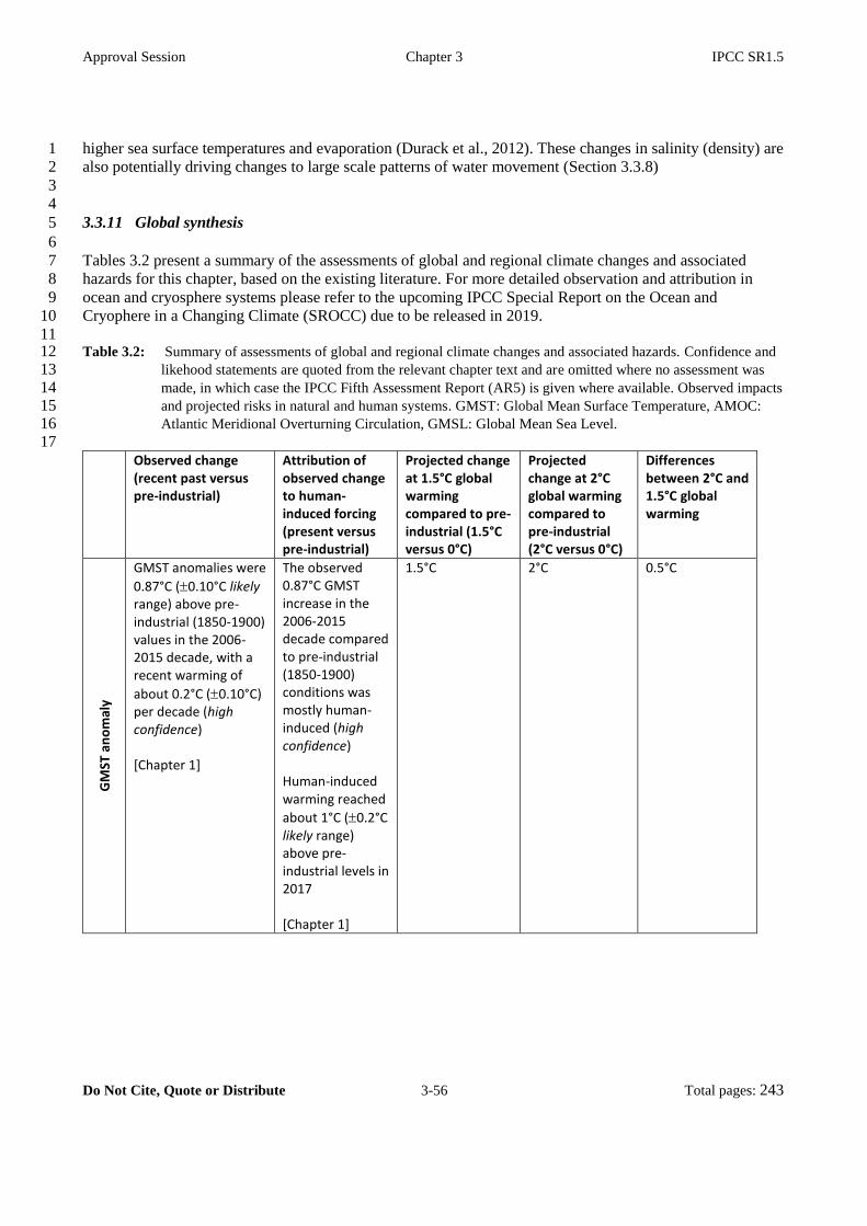
Approval Session Chapter 3 IPCC SR1.5
Do Not Cite, Quote or Distribute 3-56 Total pages: 243
higher sea surface temperatures and evaporation (Durack et al., 2012). These changes in salinity (density) are 1
also potentially driving changes to large scale patterns of water movement (Section 3.3.8) 2
3
4
3.3.11 Global synthesis 5
6
Tables 3.2 present a summary of the assessments of global and regional climate changes and associated 7
hazards for this chapter, based on the existing literature. For more detailed observation and attribution in 8
ocean and cryosphere systems please refer to the upcoming IPCC Special Report on the Ocean and 9
Cryophere in a Changing Climate (SROCC) due to be released in 2019. 10
11 Table 3.2: Summary of assessments of global and regional climate changes and associated hazards. Confidence and 12
likehood statements are quoted from the relevant chapter text and are omitted where no assessment was 13 made, in which case the IPCC Fifth Assessment Report (AR5) is given where available. Observed impacts 14 and projected risks in natural and human systems. GMST: Global Mean Surface Temperature, AMOC: 15 Atlantic Meridional Overturning Circulation, GMSL: Global Mean Sea Level. 16
17
Observed change (recent past versus pre-industrial)
Attribution of observed change to human-induced forcing (present versus pre-industrial)
Projected change at 1.5°C global warming compared to pre-industrial (1.5°C versus 0°C)
Projected change at 2°C global warming compared to pre-industrial (2°C versus 0°C)
Differences between 2°C and 1.5°C global warming
GM
ST a
no
mal
y
GMST anomalies were
0.87°C (0.10°C likely range) above pre-industrial (1850-1900) values in the 2006-2015 decade, with a recent warming of
about 0.2°C (0.10°C) per decade (high confidence) [Chapter 1]
The observed 0.87°C GMST increase in the 2006-2015 decade compared to pre-industrial (1850-1900) conditions was mostly human-induced (high confidence) Human-induced warming reached
about 1°C (0.2°C likely range) above pre-industrial levels in 2017 [Chapter 1]
1.5°C 2°C 0.5°C

Approval Session Chapter 3 IPCC SR1.5
Do Not Cite, Quote or Distribute 3-57 Total pages: 243
Observed change (recent past versus pre-industrial)
Attribution of observed change to human-induced forcing (present versus pre-industrial)
Projected change at 1.5°C global warming compared to pre-industrial (1.5°C versus 0°C)
Projected change at 2°C global warming compared to pre-industrial (2°C versus 0°C)
Differences between 2°C and 1.5°C global warming
Tem
pe
ratu
re e
xtre
me
s
Overall decrease in the number of cold days and nighs and an overall increase in the number of warm days and nights at the global scale on land (very likely) Continental-scale increase in intensity and frequency of hot days and nights, and decrease in intensity and frequency of cold day and nights, in North America, Europe and Australia. (very likely) Increases in frequency or duration of warm spell lengths in large parts of Europe, Asia and Australia (high confidence (likely)), as well as on global scale (medium confidence) [Section 3.3.2]
Anthropogenic forcing has contributed to the observed changes in the frequency and intensity of daily temperature extremes on the global scale since the mid-20th century (very likely) [Section 3.3.2]
Global-scale increased intensity and frequency of hot days and nights, and decreased intensity and frequency of cold days and nights (very likely) Warming of temperature extremes highest over land, including many inhabited regions (high confidence), with increases of up to 3°C in mid-latitude warm season, and up to 4.5 in high-latitude cold season (medium confidence) Highest increase of frequency of unusually hot extremes in tropical regions (medium confidence) [Section 3.3.2]
Global-scale increased intensity and frequency of hot days and nights, and decreased intensity and frequency of cold days and nights (very likely) Warming of temperature extremes highest over land, including many inhabited regions (high confidence), with increases of up to 4°C in mid-latitude warm season, and up to 6°C in high-latitude cold season (medium confidence) Highest increase of frequency of unusually hot extremes in tropical regions (medium confidence) [Section 3.3.2]
Global-scale increased intensity and frequency of hot days and nights, and decreased intensity and frequency of cold days and nights (high confidence) Global-scale increase in length of warm spells and decrease in length of cold spells (high confidence)
Strongest increase in frequency for rarest and most extreme events (high confidence) Particularly large increases in hot extremes in inhabited regions (high confidence) [Section 3.3.2]

Approval Session Chapter 3 IPCC SR1.5
Do Not Cite, Quote or Distribute 3-58 Total pages: 243
Observed change (recent past versus pre-industrial)
Attribution of observed change to human-induced forcing (present versus pre-industrial)
Projected change at 1.5°C global warming compared to pre-industrial (1.5°C versus 0°C)
Projected change at 2°C global warming compared to pre-industrial (2°C versus 0°C)
Differences between 2°C and 1.5°C global warming
He
avy
pre
cip
itat
ion
More areas with increases than decreases in the frequency, intensity and/or amount of heavy precipitation (likely) [Section 3.3.3]
Human influence contributed to global-scale tendency towards increases in the frequency, intensity and/or amount of heavy precipitation events (medium confidence) [Section 3.3.3]
Increases in frequency, intensity and/or amount heavy precipitation when averaged on global land, with positive trends in several regions (high confidence) [Section 3.3.3]
Increases in frequency, intensity and/or amount heavy precipitation when averaged on global land, with positive trends in several regions (high confidence) [Section 3.3.3]
Higher frequency, intensity and/or amount of heavy precipitation when averaded on global on land at 2°C versus 1.5°C (high confidence) Several regions are projected to experience increases in heavy precipitation at 2°C warming versus 1.5°C (high confidence), in particular in high-latitude and mountainous regions, as well as in Eastern Asia and Eastern North America (medium confidence) [Section 3.3.3]

Approval Session Chapter 3 IPCC SR1.5
Do Not Cite, Quote or Distribute 3-59 Total pages: 243
Observed change (recent past versus pre-industrial)
Attribution of observed change to human-induced forcing (present versus pre-industrial)
Projected change at 1.5°C global warming compared to pre-industrial (1.5°C versus 0°C)
Projected change at 2°C global warming compared to pre-industrial (2°C versus 0°C)
Differences between 2°C and 1.5°C global warming
Dro
ugh
t an
d d
ryn
ess
High confidence in dryness trends in some regions, especially drying in Mediterranean region (including Southern Europe, Northern Africa and the Near-East) Low confidence in drought and dryness trends at global scale. [Section 3.3.4]
Medium confidence in attribution of drying trend in Southern Europe Mediterranean region Low confidence elsewhere, in part due to large interannual variability and longer duration (and thus lower frequency) of drought events, as well as to dependency on dryness index definition [Section 3.3.4]
Medium confidence of drying trends in Mediterranean region. Low confidence elsewhere, in part due to large interannual variability and longer duration (and thus lower frequency) of drought events, as well as to dependency on dryness index definition [Section 3.3.4]
Medium confidence of drying trends in Mediterranean region and South Africa. Low confidence elsewhere, in part due to large interannual variability and longer duration (and thus lower frequency) of drought events, as well as to dependency on dryness index definition [Section 3.3.4]
Medium confidence of stronger drying trends in Mediterranean region and South Africa at 2°C versus 1.5°C global warming. Low confidence elsewhere, in part due to large interannual variability and longer duration (and thus lower frequency) of drought events, as well as to dependency on dryness index definition [Section 3.3.4]
Ru
no
ff &
riv
er
flo
od
ing
Streamflow trends mostly non-statistically significant (high confidence) Increase in flood frequency and extreme streamflow in some regions (high confidence) [Section 3.3.5]
Not assessed in this report.
Expansion of the global land area with significant increase in runoff (medium confidence) Increase in flood hazard in some regions (medium confidence)
[Section 3.3.5]
Expansion of the global land area with significant increase in runoff (medium confidence) Increase in flood hazard in some regions (medium confidence) [Section 3.3.5]
Expansion of the global land area with significant increase in runoff (medium confidence) Expansion in the area affected by flood hazard (medium confidence) [Section 3.3.5]
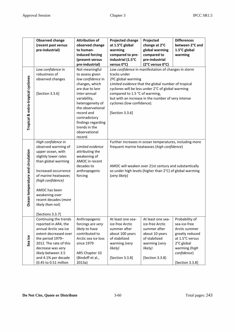
Approval Session Chapter 3 IPCC SR1.5
Do Not Cite, Quote or Distribute 3-60 Total pages: 243
Observed change (recent past versus pre-industrial)
Attribution of observed change to human-induced forcing (present versus pre-industrial)
Projected change at 1.5°C global warming compared to pre-industrial (1.5°C versus 0°C)
Projected change at 2°C global warming compared to pre-industrial (2°C versus 0°C)
Differences between 2°C and 1.5°C global warming
Tro
pic
al &
ext
ra-t
rop
ical
cyc
lon
es
Low confidence in robustness of observed changes [Section 3.3.6]
Not meaningful to assess given low confidence in changes, which are due to lare inter-annual variability, heterogeneity of the observational record and contradictory findings regarding trends in the observational record.
Low confidence in manifestation of changes in storm tracks under 2ºC global warming Limited evidence that the global number of tropical cyclones will be less under 2°C of global warming compared to 1.5 °C of warming, but with an increase in the number of very intense cyclones (low confidence). [Section 3.3.6]
Oce
an t
em
pe
ratu
re a
nd
cir
cula
tio
n
High confidence in observed warming of upper ocean, with slightly lower rates than global warming Increased occurrence of marine heatwaves (high confidence) AMOC has been weakening over recent decades (more likely than not) [Sections 3.3.7]
Limited evidence attributing the weakening of AMOC in recent decades to anthropogenic forcing
Further increases in ocean temperatures, including more frequent marine heatwaves (high confidence) AMOC will weaken over 21st century and substantically so under high levels (higher than 2°C) of global warming (very likely)
Sea
ice
Continuing the trends reported in AR4, the annual Arctic sea ice extent decreased over the period 1979–2012. The rate of this decrease was very likely between 3.5 and 4.1% per decade (0.45 to 0.51 million
Anthropogenic forcings are very likely to have contributed to Arctic sea ice loss since 1979 AR5 Chapter 10 (Bindoff et al., 2013a)
At least one sea-ice-free Arctic summer after about 100 years of stabilized warming (very likely) [Section 3.3.8]
At least one sea-ice-free Arctic summer after about 10 years of stabilized warming (very likely) [Section 3.3.8]
Probability of sea-ice-free Arctic summer greatly reduced at 1.5°C versus 2°C global warming (high confidence) [Section 3.3.8]

Approval Session Chapter 3 IPCC SR1.5
Do Not Cite, Quote or Distribute 3-61 Total pages: 243
Observed change (recent past versus pre-industrial)
Attribution of observed change to human-induced forcing (present versus pre-industrial)
Projected change at 1.5°C global warming compared to pre-industrial (1.5°C versus 0°C)
Projected change at 2°C global warming compared to pre-industrial (2°C versus 0°C)
Differences between 2°C and 1.5°C global warming
km2 per decade) AR5 Chapter 4 (Vaughan et al., 2013)
Intermediate temperature overshoot has no long-term consequences for Arctic sea-ice cover (high confidence) 3.3.8
Sea
leve
l
It is likely that the rate of GMSL has continued to increase since the early 20th century, with estimates that range from 0.000 [–0.002 to 0.002] mm yr–2 to 0.013 [0.007 to 0.019] mm yr–2 AR5 Chapter 13 (Church et al., 2013)
It is very likely that there is a substantial contribution from anthropogenic forcings to the global mean sea level rise since the 1970s AR5 Chapter 10 (Bindoff et al., 2013a)
Not assessed in this report
Not assessed in this report
GMSL rise will be about 0.1 m less at 1.5°C versus 2°C global warming (medium confidence) [Section 3.3.9]
Oce
an c
he
mis
try
Ocean acidification due to increased CO2 has resulted in 0.1 pH unit decrease since the pre-industrial period which is unprecedented in the last 35 Ma (high confidence) [Section 3.3.10]
It is very likely) that oceanic uptake of anthropogenic CO2 has resulted in acidification of surface waters. [Section 3.3.10]
Ocean chemistry is changing with global temperature with impacts projected at 1.5°C and, more so, at 2°C (high agreement, medium evidence) [Section 3.3.10]
1

Approval Session Chapter 3 IPCC SR1.5
Do Not Cite, Quote or Distribute 3-62 Total pages: 243
Observed impacts and projected risks in natural and human systems 1
2
3.4.1 Introduction 3
4
In Section 3.4, we explore the new literature and update the assessment of impacts and projected risks into 5
the future for a large number of natural and human systems. We also explore adaptation opportunities laying 6
the steps for reducing climate change, preparing the ground for later discussions on the opportunities to 7
tackle both mitigation and adaptation while at the same time recognising the importance of sustainable 8
development and reducing the inequities among people and societies facing climate change. 9
10
Working Group II (WGII) of the IPCC Fifth Assessment Report (AR5) provided an assessment of the 11
literature for climate risk for natural and human systems across a wide range of environments, sectors and 12
greenhouse gas scenarios, as well as for particular geographic regions (IPCC, 2014a, 2014b). The 13
comprehensive assessment undertaken by AR5 evaluated the evidence of changes to natural systems, and the 14
impact on human communities and industry. While impacts varied substantially between systems, sectors 15
and regions, many changes over the past 50 years can be attributed to human driven climate change and its 16
impacts. In particular, risks were observed by AR5 to be increasing for natural ecosystems as climate 17
extremes increase in frequency and intensity, as well as those associated with fauna and flora shifting their 18
biogeographical ranges to higher latitudes and altitudes, with consequences for ecosystem services and 19
human dependence. AR5 also reported increasing evidence of changing patterns of disease, invasive species, 20
as well as growing risks for coastal communities and industry, especially important when it comes to sea 21
level rise and human vulnerability. 22
23
One of the strong themes that has emerged from AR5 was that previous assessments may have under-24
estimated how sensitive natural and human systems are to climate change. A more recent analysis of 25
attribution to greenhouse gas forcing at the global scale (Hansen and Stone, 2016) has confirmed that many 26
impacts related to changes in regional atmospheric and ocean temperature can be confidently attributed to 27
anthropogenic forcing, while attribution to anthropogenic forcing of those related to precipitation are by 28
comparison less clear. Moreover there is no strong direct relationship between the robustness of climate 29
attribution and that of impact attribution (Hansen and Stone, 2016). The observed changes in human systems 30
are increased by the loss of ecosystem services (e.g. reduced access to safe water) that are supported by 31
biodiversity (Cramer et al., 2014). Limited research on the risks of warming of +1.5 and +2C was conducted 32
following AR5 for most key economic sectors and services, for livelihoods and poverty, and for rural areas. 33
For these systems, climate is one of many drivers that result in adverse outcomes. Other factors include 34
patterns of demographic change, socioeconomic development, trade, and tourism. Further, consequences of 35
climate change for infrastructure, tourism, migration, crop yields, and other impacts interact with underlying 36
vulnerabilities, such as for individuals and communities engaged in pastoralism, mountain farming, and 37
artisanal fisheries, to affect livelihoods and poverty (Dasgupta et al., 2014). 38
39
Incomplete data and understanding of these lower end climate scenarios has increased the request for greater 40
data and understanding of the projected risks of warming of 1.5°C, and 2°C for reference. This section 41
explores the available literature on the projected risks, impacts and adaptation options, and is supported by 42
additional information and background in Supplemantary Material (3.SM3, 3.SM;3.1, 3.SM.3.2, 3.SM.3.4, 43
3.SM.3.5, S3-4-12). A description of the main assessment methods of this chapter is given in Section 3.2.2. 44
45
46

Approval Session Chapter 3 IPCC SR1.5
Do Not Cite, Quote or Distribute 3-63 Total pages: 243
3.4.2 Freshwater resources (quantity and quality) 1
2
Water availability 3
WGII AR5 concluded that about 80% of the world’s population already suffers from serious threats to its 4
water security as measured by indicators including water availability, water demand, and pollution 5
(Vörösmarty et al., 2010). UNESCO (2011) concluded that climate change can alter the availability of water 6
and threaten water security. 7
8
Although physical changes on streamflow and continental runoff that are consistent with climate change 9
have been identified (Section 3.3.5), water scarcity in the past is still less well understood because the 10
scarcity assessment needs to take into account various factors such as the operations of water supply 11
infrastructure and human water use behaviour (Mehran et al., 2017), as well as incorporating green water, 12
water quality, and environmental flow requirements (J. Liu et al., 2017). Over the past century, substantial 13
growth in population, industrial and agricultural activities, and living standards have exacerbated water stress 14
in many parts of the world, especially in semi-arid and arid regions such as California in the US 15
(AghaKouchak et al., 2015; Mehran et al., 2015). Due to changes in climate and water consumption 16
behavior, and particularly the effects of spatial distribution of population growth relative to water resources, 17
the population under water scarcity increased from 0.24 billion (14% of global population) in the 1900s to 18
3.8 billion (58%) in the 2000s. In that last period (2000s), 1.1 billion people (17% of global population) 19
mostly living in South and East Asia, North Africa and Middle East were facing high water shortage and 20
high water stress (Kummu et al., 2016). 21
22
Over the next few decades, and for increases in global mean temperature of less than about 2ºC, the AR5 23
concluded that changes in population will generally have a greater effect on water resource availability than 24
changes in climate. Climate change, however, will regionally exacerbate or offset the effects of population 25
pressure (Jiménez Cisneros et al., 2014). 26
27
The differences in projected changes in runoff under 1.5ºC and 2ºC, particularly those that are regional, are 28
described in Section 3.3.5. Constraining to 1.5ºC instead of 2ºC warming can mitigate the risks on water 29
availability although socio-economic drivers could affect the availability more than the risks posed by the 30
variation in warming levels, while the risks found in regions are not homogeneous (medium evidence, 31
medium agreement) (Gerten et al., 2013; Hanasaki et al., 2013; Arnell and Lloyd-Hughes, 2014; Schewe et 32
al., 2014; Karnauskas et al., 2018). Assuming a constant population in these models, Gerten et al. (2013) 33
reveal that an additional 8% of the world population in 2000 will be exposed to new or aggravated water 34
scarcity at 2ºC warming. This value is almost halved - with 50 % larger reliability - when warming is 35
constrained to 1.5ºC. People inhabiting river basins particularly in the Middle East and Near East become 36
newly exposed to chronic water scarcity even if the warming is constrained under 2ºC warming. Many 37
regions especially in Europe, Australia and southern Africa appear to be affected at 1.5ºC if the reduction in 38
water availability is computed for non-water scarce basins in addition to the reductions in water-scarce 39
regions. From a contemporary population of approximately 1.3 billion exposed to water scarcity, about 3% 40
(North America) to 9% (Europe) are prone to aggravated scarcity at 2ºC warming (Gerten et al., 2013). 41
Under the Shared Socioeconomic Pathway (SSP)2 population scenario, about 8% of the global population 42
are projected to experience a severe reduction in water resources under warming of 1.7ºC in 2021-2040, 43
increasing to 14 % of the population under 2.7ºC in 2043-2071, based on either the criteria of discharge 44
reduction >20% or >1 standard deviation (Schewe et al., 2014). Depending on the scenarios of SSP1 to 5, 45
exposure to the increase of water scarcity in 2050 will be globally reduced by 184–270 million people at 46
about 1.5ºC compared to the impacts at about 2ºC. However the variation between socio-economic 47

Approval Session Chapter 3 IPCC SR1.5
Do Not Cite, Quote or Distribute 3-64 Total pages: 243
differences is larger than the variation between warming levels (Arnell and Lloyd-Hughes, 2014). 1
2
On many small developing islands, there will be freshwater stress derived from projected aridity change, 3
however, constraining to 1.5ºC warming can avoid a substantial fraction of water stress compared to 2ºC, 4
especially across the Caribbean region, particularly on the island of Hispaniola (Dominican Republic and 5
Haiti) (Karnauskas et al. (2018). Hanasaki et al. (2013) conclude that the projected range of changes in 6
global irrigation water withdrawal (relative to the baseline of 1971-2000) with human configuration fixing 7
non-meteorological variables at the period of about 2000 are 1.1–2.3% and 0.6–2.0% lower at 1.5ºC than at 8
2ºC, respectively. The same study, Hanasaki et al. (2013) reports on the importance of water use scenarios in 9
water scarcity assessments, but neither quantitative nor qualitative information regarding water use are 10
available. Hanasaki et al. (2013) conclude that the projected ranges of changes in global irrigation water 11
withdrawal with human configuration fixing non-meteorological variables at about 2000 are 1.1–2.3% at 12
about 1.5ºC, which is projected by Geophysical Fluid Dynamic Laboratory (GFDL) model (Representative 13
Concentration Pathway (RCP)2.6 in 2071-2100 and RCP4.5 in 2011-2040), and 0.6–2.0% at about 2ºC 14
according to the projection using the Hadley Centre New Global Environmental Model (HadGEM) and 15
Model for Interdisciplinary Research on Climate (MIROC) models (RCP4.5 and RCP8.5 in 2011-2040, 16
respectively). 17
18
Comparing the impacts on hydropower production at 1.5°C and 2°C, it is found that mean gross potential 19
increases in northern, eastern and western Europe, and decreases in southern Europe (Tobin et al., 2018; 20
Jacob et al., 2018). The Baltic and Scandinavian countries will have the most positive impacts on production. 21
The most negatively impacted are Greece, Spain, and Portugal, although the impacts can be reduced by 22
limiting warming at 1.5°C (Tobin et al., 2018). It is found that, in Greece, Spain and Portugal, a warming of 23
2°C will decrease hydropower potential below 10%, while limiting to 1.5°C warming will keep the reduction 24
to 5% or less. There is however, substantial uncertainty associated with these results due to a large spread 25
between the climate models (Tobin et al., 2018). 26
27
Due to a combination of higher water temperatures and reduced summer river flows, the usable capacity of 28
thermoelectric power plants using river water for cooling is expected to reduce in all European countries 29
(Tobin et al., 2018; Jacob et al., 2018), with the magnitude of decreases being about 5% for 1.5°C and 10% 30
for 2°C for most European countries (Tobin et al., 2018). Greece, Spain, and Bulgaria will have the largest 31
reduction at 2°C (Tobin et al., 2018). 32
33
Fricko et al. (2016) assess the direct global energy sector water use across a broad range of energy system 34
transformation pathways in order to identify the water impacts of a 2°C climate policy. This study revealed 35
that there will be substantial divergence in water withdrawal for thermal power plant cooling under a 36
condition in which the distribution of future cooling technology for energy generation is fixed, whereas 37
adopting alternative cooling technologies and water resources will make the divergence considerably 38
smaller. 39
40
Extreme hydrological events (floods and droughts) 41
WGⅡAR5 concluded that socio-economic losses from flooding since the mid-20th century have increased 42
mainly due to greater exposure and vulnerability (high confidence; Jiménez Cisneros et al., 2014). There is 43
low confidence due to limited evidence, however, that anthropogenic climate change has affected the 44
frequency and the magnitude of floods. WGII AR5 also concluded that there is no evidence that surface 45
water and groundwater drought frequency has changed over the last few decades, although impacts of 46
drought have increased mostly due to increased water demand (Jiménez Cisneros et al., 2014). 47
Approval Session Chapter 3 IPCC SR1.5
Do Not Cite, Quote or Distribute 3-65 Total pages: 243
1
Since the AR5, the number of studies related to river flooding and meteorological drought based on long-2
term observed data have been gradually increasing. There has been progress since the AR5 in identifying 3
historical changes in streamflow and continental runoff (Section 3.3.5). As a result of population and 4
economic growth, increased exposure of people and assets has caused more damage due to flooding. 5
However, differences in flood risks among regions reflect the balance among the magnitude of the flood, 6
population, their vulnerabilities, the value of assets affected by flooding, and the capacity to cope with flood 7
risks that depend on socio-economic development conditions as well as topography and hydro-climatic 8
conditions (Tanoue et al., 2016). The AR5 assessment concluded that there was low confidence in the 9
attribution of global changes in droughts (Bindoff et al., 2013b). However, recent publications based on 10
observational and modeling evidence assessed that human emissions have substantially increased the 11
probability of drought years in the Mediterranean region (Sections 3.3.4). 12
13
WGII AR5 assessed that global flood risk will increase in the future partly due to climate change (limited 14
evidence, medium agreement), with projected changes in the frequency of droughts longer than 12 months 15
being more uncertain, because of their dependence on accumulated precipitation over long periods (Jiménez 16
Cisneros et al., 2014). 17
18
Increases in the risks associated with runoff at global scale (high confidence), and in flood hazard in some 19
regions (high confidence), can be expected at warming of 1.5°C level with an overall increase in the area 20
affected by flood hazard at 2°C (high confidence) (see Section 3.3.5). There are studies, however, revealing 21
that socio-economic conditions will exacerbate flood impacts more than global climate change, and the 22
magnitude of the impacts can be larger in some region (Arnell and Lloyd-Hughes, 2014; Winsemius et al., 23
2016; Alfieri et al., 2017; Arnell et al., 2018; Kinoshita et al., 2018) (limited evidence, medium agreement). 24
Assuming constant population sizes, countries representing 73% of the world population will experience 25
increasing flood risk with an average of 580% increase at 4ºC compared to the impact simulated over the 26
baseline period 1976-2005. Such impact is projected to be reduced to 100% increase at 1.5ºC and 170% at 27
2ºC (Alfieri et al., 2017). Alfieri et al. (2017) reveal that the largest increases in flood risks are found in U.S., 28
Asia, and Europe in general, while decreases are found in only few countries in Eastern Europe and Africa. 29
Alfiere et al (2017) report that the projected changes are not homogeneously distributed on the world land 30
surface. Alfieri et al. (2018) studied the population affected by flood events in European states, specifically 31
Central and Western Europe, and found that the population affected can be limited to 86% for 1.5ºC 32
warming compared to 93% at 2ºC. Under the SSP2 population scenario, Arnell et al. (2018) find that 39% 33
(range 36-46%) of impacts on populations exposed to river flood can be globally avoided at 1.5ºC compared 34
to 2 ºC warming. 35
36
Under SSP1-5 scenario, Arnell and Lloyd-Hughes (2014) find that the number of people exposed to 37
increased flooding in 2050 under warming of about 1.5ºC can be reduced by 26–34 million compared to 38
those people exposed to increased flooding associated with 2ºC. Variation between socio-economic 39
differences, however, are larger than the variation between the extent of global warming. Kinoshita et al. 40
(2018) find that a serious increase in potential flood fatality (5.7%) is projected without any adaptation if 41
global warming increases from 1.5ºC to 2ºC, whereas an increase in potential economic loss (0.9%) is 42
relatively small. Nevertheless, the study indicates that socio-economic changes have a stronger contribution 43
to the potentially increased consequences of future floods, and about a half of the increase of potential 44
economic losses is mitigated by autonomous adaptation. 45
46
There is limited information about the global and regional projected risks posed by droughts at 1.5ºC and 47

Approval Session Chapter 3 IPCC SR1.5
Do Not Cite, Quote or Distribute 3-66 Total pages: 243
2ºC. However, hazards by droughts under 1.5ºC can be reduced compared to the hazards at 2ºC (Section 1
3.3.4). Under constant socio-economic conditions, the population exposed to drought at 2ºC warming is 2
projected to be larger than at 1.5ºC (Smirnov et al., 2016; Sun et al., 2017; Arnell et al., 2018; Liu et al., 3
2018) (limited evidence, medium agreement). Under the same scenario, the global mean monthly number of 4
people expected to be exposed to extreme drought at 1.5ºC in 2021-2040 is projected to be 114.3 million 5
people while 190.4 million people at 2ºC in 2041-2060 (Smirnov et al., 2016) . Under the SSP2 population 6
scenario, Arnell et al. (2018) project that 39% (range 36-51%) of impacts on populations exposed to drought 7
can be globally avoided at 1.5ºC compared to 2ºC. 8
9
Liu et al. (2018) study the changes in population exposure to severe droughts in 27 regions and around the 10
globe for 1.5ºC and 2ºC warming using the SSP1 population scenario, compared to the baseline period of 11
1986-2005, and conclude that urban population exposure in most regions can be decreased at 1.5ºC 12
(350.2±158.8 million) compared to 2ºC (410.7±213.5 million), respectively. Liu et al. (2018) also suggest 13
that more urban populations will be exposed to severe droughts in Central Europe, Southern Europe, the 14
Mediterranean, West Africa, East and West Asia and Southeast Asia, and the number of the affected people 15
will escalate further in these regions at 2ºC. In the Haihe River Basin in China, the proportion of the 16
population exposed to droughts at 1.5ºC is projected to be reduced by 30.4%, but increased by 74.8% at 2°C 17
relative to 339.65 million people in the 1986–2005 period (Sun et al., 2017) . 18
19
Alfieri et al. (2018) estimate expected damage from flood at the European level for the baseline period (1976-20
2005), in which the reported annual figure is 5 billion euro of losses and reveal that relative changes of flood 21
impacts rise with warming levels from 116% at 1.5°C to 137% at 2°C, respectively. 22
23
Kinoshita et al. (2018) study the increase of potential economic loss in SSP3 and project that the smaller loss at 24
1.5°C compared to at 2°C (0.9%) is marginal regardless of whether the vulnerability is fixed at the current level 25
or not. Winsemius et al. (2016) show adaptation measures have the potential to greatly reduce present and future 26
flood damage, by analyzing the differences in results with and without flood protection standard. They conclude 27
that increases in flood induced economic impacts (% Gross Domestic Product, GDP) in African countries are 28
mainly driven by climate change and Africa’s growing assets become increasingly exposed to floods. And hence 29
there is greater need for long-term and sustainable investments in adaptation in Africa. 30
31
Groundwater 32
WGII AR5 concluded that the detection of changes in groundwater systems, and attribution of those changes 33
to climatic changes, are rare owing to a lack of appropriate observation wells and an overall small number of 34
studies (Jiménez Cisneros et al., 2014). 35
36
Since AR5, the number of studies based on long-term observed data continues to be limited. The 37
groundwater-fed lakes in north-eastern central Europe have been affected by climate and land use changes, 38
and show a predominantly negative lake-level trend in 1999–2008 (Kaiser et al., 2014). 39
40
WGII AR5 concluded that climate change is projected to reduce groundwater resources significantly in most 41
dry subtropical regions (robust evidence, high agreement; Jiménez Cisneros et al., 2014). 42
43
In some regions, groundwater is often intensively used to supplement the excess demand, often leading to 44
groundwater depletion. Climate change adds further pressure on water resources and exaggerates human 45
water demands due to increasing temperatures over agricultural lands (Wada et al., 2017). Very few studies 46

Approval Session Chapter 3 IPCC SR1.5
Do Not Cite, Quote or Distribute 3-67 Total pages: 243
project the risks of groundwater depletion under 1.5ºC and 2ºC warming. Under 2ºC warming, impacts posed 1
on groundwater are projected to be greater than at 1.5ºC (limited evidence, low agreement; Portmann et al., 2
2013; Salem et al., 2017). 3
4
Portmann et al. (2013) indicate that 2.0% (range 1.1-2.6%) of global land area is projected to suffer from an 5
extreme decrease of renewable groundwater resources of more than 70% at 2ºC, which is clearly mitigated at 6
1.5ºC. The study also projects that 20% of global land surface is affected by more than 10% groundwater 7
reduction at 1.5ºC with the percentage of the land impacted increasing at 2ºC. In a groundwater-dependent 8
irrigated region in Northwest Bangladesh, the average groundwater level during the major irrigation period 9
(January-April) is projected to decrease in accordance with temperature rise (Salem et al., 2017). 10
11
Water quality 12
WGII AR5 concluded that most observed changes to water quality from climate change are from isolated 13
studies, mostly of rivers or lakes in high-income countries, using a small number of variables (Jiménez 14
Cisneros et al., 2014). The AR5 report assessed that climate change is projected to reduce raw water quality, 15
posing risks to drinking water quality with conventional treatment (medium evidence, high agreement; 16
Jiménez Cisneros et al. (2014). 17
18
Since AR5, studies have detected climate change impacts on several indices of water quality in lakes, 19
watershed and regional (e.g., Patiño et al., 2014; Aguilera et al., 2015; Watts et al., 2015; Marszelewski and 20
Pius, 2016; Capo et al., 2017). Since WGII AR5, the number of studies utilizing RCP scenarios at regional or 21
watershed scale have been gradually increased (e.g., Boehlert et al., 2015; Teshager et al., 2016; 22
Marcinkowski et al., 2017). There are, however, few studies that explore projected impacts on water quality 23
under 1.5ºC versus 2ºC warming. Differences in impacts on water quality between 1.5ºC and 2ºC warming is 24
unclear (Bonte and Zwolsman, 2010; Hosseini et al., 2017) (limited evidence, low agreement). The daily 25
probability of exceeding the chloride standard for drinking water taken from Lake IJsselmeer (Andijk, the 26
Netherlands) is projected to increase about five times at 2ºC relative to 1ºC since 1990 (Bonte and 27
Zwolsman, 2010). Mean monthly dissolved oxygen concentrations and nutrient concentrations in the upper 28
Qu’Appelle River (Canada) in 2050-2055 are projected to decrease less at about 1.5ºC warming (RCP2.6 in 29
2050-2055) compared to about 2ºC (RCP4.5 in 2050-2055) (Hosseini et al., 2017). In the three river basins 30
(Sekong, Sesan, and Srepok in southeast Asia) about 2ºC warming (1.05 ºC increase in the 2030s relative to 31
the baseline peiod 1981-2008, RCP8.5), impacts posed by land-use change on water quality is projected to 32
be greater than at 1.5ºC (0.89 ºC increase in the 2030s relative to the baseline peiod 1981-2008, 33
RCP4.5)(Trang et al., 2017). Under the same warming scenario, Trang et al. (2017) project annual nitrogen 34
(N) and phosphorus (P) yields change in 2030s at about 1.5ºC and about 2ºC as well as with combinations of 35
two land-use change scenarios: 1) conversion of forest to grassland, and 2) of forest to agricultural land. The 36
projected changes in N (P) yield under 1.5ºC and 2ºC scenarios are 7.3 (5.1)% and -6.6 (-3.6)%, whereas 37
under the combination of land-use scenarios are 1) 5.2 (12.6)% and 8.8 (11.7)%, and 2) 7.5 (14.9)% and 38
3.7(8.8)%, respectively (Trang et al., 2017). 39
40
Soil erosion and sediment load 41
WGII AR5 concluded that there is little or no observational evidence that soil erosion and sediment load 42
have been altered significantly due to climate change (limited evidence, medium agreement), (Jiménez 43
Cisneros et al., 2014). As studies of climate change impacts on soil erosion have increased where rainfall is 44
an important driver (Lu et al., 2013), studies have increasingly considered other factors such as rainfall 45
intensity (e.g., Shi and Wang, 2015; Li and Fang, 2016), snow melt, and change of vegetation cover due to 46
temperature rise (Potemkina and Potemkin, 2015), and crop management practices (Mullan et al., 2012). 47

Approval Session Chapter 3 IPCC SR1.5
Do Not Cite, Quote or Distribute 3-68 Total pages: 243
WGII AR5 concluded that increases in heavy rainfall and temperature are projected to change soil erosion 1
and sediment yield, although the extent of these changes is highly uncertain and depends on rainfall 2
seasonality, land cover, and soil management practices (Jiménez Cisneros et al., 2014). 3
4
While published studies of climate change impacts on soil erosion have increased since 2000 globally (Li 5
and Fang, 2016), few articles have addressed impacts at 1.5ºC and 2ºC warming. The existing studies have 6
found few differences in projected risks posed on sediment load under 1.5ºC and 2ºC (limited evidence, low 7
agreement; Cousino et al., 2015; Shrestha et al., 2016). The differences between average annual sediment 8
load under 1.5ºC and 2ºC warmings are not clear because of complex interactions among climate change, 9
land cover/surface and soil management (Cousino et al., 2015; Shrestha et al., 2016). Averages of annual 10
sediment load are projected to be similar under 1.5ºC and 2ºC , in particular in the Great Lakes region in the 11
US as well as in the Lower Mekong region in Southeast Asia (Cousino et al., 2015; Shrestha et al., 2016). 12
13
14
3.4.3 Terrestrial and wetland ecosystems 15
16
Biome shifts 17
Latitudinal and elevational shifts of biomes (major ecosystem types) boreal, temperate, and tropical regions 18
have been detected (Settele et al., 2014, AR5) and new studies confirm this (e.g. for shrub encroachment on 19
tundra; Larsen et al., 2014). Attribution studies indicate that anthropogenic climate change has made a 20
greater contribution to these changes than any other factor (Settele et al., 2014, medium confidence). 21
22
An ensemble of seven Dynamic Vegetation Models driven by projected climates from 19 alternative General 23
Circulation Models (GCMs) (Warszawski et al., 2013 shows 13% (range 8-20%) of biomes transforming at 24
2°C warming, but only 4% (range 2-7%) doing so at 1°C; suggesting that about 7% may be transformed at 25
1.5°C, indicating a doubling of the areal extent of biome shifts between 1.5ºC and 2°C warming (Figure 26
3.15a). A single ecosystem model LPJmL (Gerten et al., 2013) illustrates that biome shifts in the Arctic, 27
Tibet, Himalayas, South Africa and Australia would be avoided by constraining warming to 1.5°C as 28
compared with 2°C (Figure 3.15b). Seddon et al. (2016) quantitatively identified ecologically sensitive 29
regions to climate change in most of the continents from tundra to tropical rainforest. Biome transformation 30
may in some cases be associated with novel climates and ecological communities (Prober et al., 2012). 31
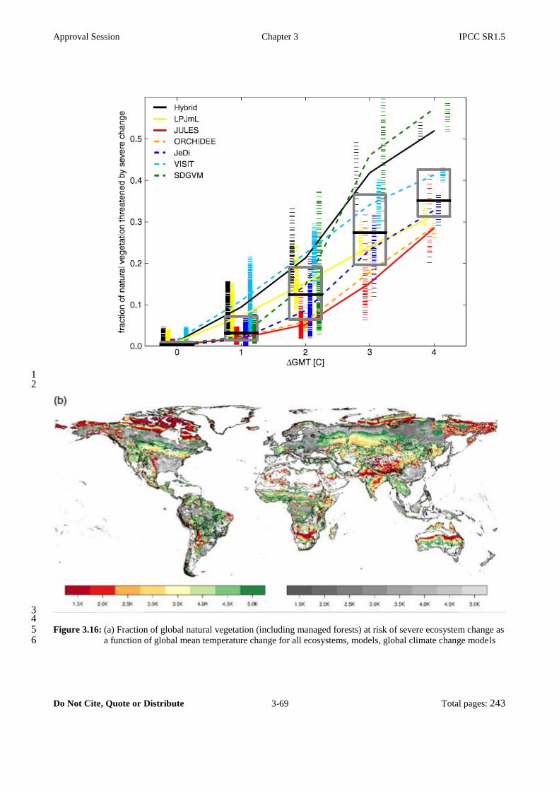
Approval Session Chapter 3 IPCC SR1.5
Do Not Cite, Quote or Distribute 3-69 Total pages: 243
1 2
3 4
Figure 3.16: (a) Fraction of global natural vegetation (including managed forests) at risk of severe ecosystem change as 5 a function of global mean temperature change for all ecosystems, models, global climate change models 6
Approval Session Chapter 3 IPCC SR1.5
Do Not Cite, Quote or Distribute 3-70 Total pages: 243
and Representative Concentration Pathways (RCPs). The colours represent the different ecosystem 1 models, which are also horizontally separated for clarity. Results are collated in unit-degree bins, where 2 the temperature for a given year is the average over a 30-year window centred on that year. The boxes 3 span the 25th and 75th percentiles across the entire ensemble. The short, horizontal stripes represent 4 individual (annual) data points, the curves connect the mean value per ecosystem model in each bin. The 5 solid (dashed) curves are for models with (without) dynamic vegetation composition changes. Source: 6 (Warszawski et al., 2013) (b) Threshold level of global temperature anomaly above pre-industrial levels 7 that leads to significant local changes in terrestrial ecosystems. Regions with severe (coloured) or 8 moderate (greyish) ecosystem transformation; delineation refers to the 90 biogeographic regions. All 9 values denote changes found in >50% of the simulations. Source: (Gerten et al., 2013). Regions coloured 10 in dark red are projected to undergo severe transformation under a global warming of 1.5°C while those 11 coloured in light red do so at 2°C; other colors are used when there is no severe transformation unless 12 global warming exceeds 2°C. 13
14
15
Changes in phenology 16
Advancement in spring phenology of 2.8 ± 0.35 days per decade has been observed in plants and animals in 17
most Northern Hemisphere ecosystems in recent decades (between 30°N and 72°N), and this has been 18
attributed to changes in climate (high confidence) (Settele et al., 2014). The rates of change are particularly 19
rapid in the Arctic zone in relation with higher local warming (Oberbauer et al., 2013), but in tropical forests, 20
the phenology changes rather respond to moisture stress (Zhou et al., 2014). While a full review cannot be 21
included here, trends consistent with this earlier finding continue to be detected, including in the flowering 22
times of plants (Parmesan and Hanley, 2015), in the dates of egg laying and migration in birds (newly in 23
China, Wu and Shi, 2016), in the emergence dates of butterflies (Roy et al., 2015), and in the seasonal 24
greening-up of vegetation as detected by satellites (i.e. in the Normalised Difference Vegetation Index, 25
NDVI, Piao et al., 2015). 26
27
The potential for de-coupling of species-species interactions due to differing phenological responses to 28
climate change is well established (Settele et al., 2014) for example for plants and their insect pollinators 29
(Willmer, 2012; Scaven and Rafferty, 2013). Now, mid-century projections of plant and animal phenophases 30
in UK (Thackeray et al., 2016) clearly indicate that the timing of phenological events could change more for 31
primary consumers (6.2 days earlier on average) than for higher trophic levels (2.5-2.9 days earlier on 32
average), indicating the potential for phenological mismatch and associated risks for ecosystem functionality 33
in the future, associated with global warming of 2.1-2.7°C above pre-industrial; while differing responses 34
could alter community structure in temperate forests (Roberts et al., 2015). Here, the temperate forest 35
phenology is projected to gain 14.3 days in the near term (2010-2039) and 24.6 days in the medium term 36
(2040-2069), so in first approximation the difference between 2°C and 1.5°C global warming is about 10 37
days (Roberts et al., 2015). This phenological plasticity is not always adaptive and must be taken cautiously 38
(Duputié et al., 2015), due to accompanying changes in climate variability (risk of frost damage for plants or 39
earlier emergence of insects resulting in mortality during cold spells). Another adaptative response for the 40
plants is expanding their range with increased vigor and altered herbivore resistance in their new range, 41
analogous to invasive plants (Macel et al., 2017). 42
43
In summary, limiting warming to 1.5°C as compared with 2°C may avoid a few days of advance in spring 44
phenology and hence decrease the risks of loss of ecosystem functionality due to phenological mismatch 45
between trophic levels, and also of maladaptation coming from the sensitivity of many species to increased 46
climate variability. Nevertheless, this difference between 1.5°C and 2°C warming might be limited for plants 47
able to expand their range. 48

Approval Session Chapter 3 IPCC SR1.5
Do Not Cite, Quote or Distribute 3-71 Total pages: 243
1
Changes in species range, abundance and extinction 2
AR5 (Settele et al., 2014) concluded that the geographical ranges of many terrestrial and freshwater plant 3
and animal species have moved over the last several decades in response to warming: approximately 17 km 4
per decade poleward and 11 m up in altitude per decade. Recent trends confirm this finding, for example the 5
spatial and interspecific variance in bird populations in Europe and the North America since 1980 were 6
found to be well-predicted by trends in climate suitability (Stephens et al., 2016). Further, a recent meta-7
analysis of 27 studies concerning a total of 976 species (Wiens, 2016) found that 47% of local extinctions 8
(extirpations) reported across the globe during the 20th century could be attributed to climate change, is 9
significantly higher in tropical regions, for animals and in freshwater habitats. IUCN (2017) lists 305 10
terrestrial animal and plant species from Pacific island developing nations as being threatened by climate 11
change and severe weather. Due to lags in the responses of some species to climate change, shifts in insect 12
pollinator ranges may result in novel assemblages with unknown implications for biodiversity and ecosystem 13
function (Rafferty, 2017). 14
15
Warren et al. (2013) simulated climatically determined geographic range loss under 2°C and 4°C global 16
warming for 50,000 plant and animal species accounting for uncertainty in climate projections and for the 17
potential ability of species to disperse naturally in an attempt to track their geographically shifting climate 18
envelope. This earlier study has now been updated and expanded to incorporate 105,501 species, including 19
19,848 insects, and finds that a warming of 2°C by 2100 would lead to projected bioclimatic range losses of 20
>50% in 18 (6-35)% of 19,848 insects species, 8 (4-16)% of 12,429 vertebrate species, and 16 (9-28)% of 21
73,224 plant species studied (Warren et al., 2018b). At 1.5°C this falls to 6 (1-18) % insects, 4 (2-9)% 22
vertebrates and 8 (4-15)% plants. Hence the number of insect species projected to lose over half their 23
geographic range is reduced by two-thirds when warming is limited to 1.5°C as compared with 2°C, while 24
the number of vertebrate and plant species projected to lose over half their geographic range is halved 25
(Warren et al., 2018b). This is consistent with estimates made from an earlier study suggesting that range 26
losses at 1.5°C were significantly lower for plants than those at 2°C warming (Smith et al., 2018). It should 27
be noted that at 1.5°C warming, and if species’ ability to disperse naturally to track their preferred climate 28
geographically is inhibited by natural or anthropogenic obstacles, there still remain 10% amphibians, 8% 29
reptiles, 6% mammals, 5% birds, 10% insects and 8% plants which are projected to lose over half their 30
range, while species on average lose 20-27% of their range (Warren et al., 2018b). Since bird and mammal 31
species can disperse more easily, a small proportion can gain range as climate changes, but even at 1.5°C 32
warming the total range loss integrated over all birds and mammals greatly exceeds the integrated range gain 33
(Warren et al., 2018b). 34
35
A number of caveats are noted in studies projecting climatic range change, since the approach does not 36
incorporate the effects of extreme weather events and the role of interactions between species; and trophic 37
interactions may locally counteract range expansion of species towards higher altitudes (Bråthen et al., 38
2018). Also, there is the potential for highly invasive species to become established in new areas as climate 39
changes (Murphy and Romanuk, 2014), but there is no literature that quantifies this potential for 1.5°C 40
warming. 41
42
Pecl et al. (2017) summarize at the global level the consequences (for economic development, livelihoods, 43
food security, human health and culture) of climate-change induced species redistribution and conclude that, 44
even if anthropogenic greenhouse gas emissions stopped today, the effort for human systems to adapt to the 45
most crucial effects of climate-driven species redistribution will be far reaching and extensive. For example, 46
key insect crop pollinator families (Apidae, Syrphidae and Calliphoridae; i.e., bees, hoverflies and 47

Approval Session Chapter 3 IPCC SR1.5
Do Not Cite, Quote or Distribute 3-72 Total pages: 243
blowflies) are shown to retain significantly greater geographic ranges under 1.5°C global warming as 1
compared with 2°C (Warren et al., 2018b). In some cases when species (such as pest and disease species) 2
move into areas which become newly climatically suitable they may become invasive or harmful to human 3
or natural systems (Settele et al., 2014). Some studies are beginning to locate ‘refugial’ areas where the 4
climate remains suitable in the future for most of the species currently present: for example, (Smith et al., 5
2018) estimate that 5.5-14% more of the globe’s terrestrial land area can act as climatic refugia for plants 6
under 1.5°C warming as compared to 2°C. 7
8
There is no literature that directly estimates the proportion of species at increased risk of global (as opposed 9
to local) commitment to extinction as a result of climate change as this is difficult to quantify. However, it is 10
possible to compare the proportions of species at risk of very high range loss in Figure 2 in Warren et al. 11
(2018b) where discernibly lower number of terrestrial species projected to lose over 90% of their range at 12
1.5°C global warming as compared with 2°C; a link between very high levels of range loss and greatly 13
increased extinction risk may be inferred (Urban, 2015). Hence limiting global warming to 1.5°C as 14
compared with 2°C would be expected to reduce both range losses and associated extinction risks in 15
terrestrial species (medium confidence). 16
17
Changes in ecosystem function, biomass and carbon stocks 18
WGII AR5 (Settele et al., 2014) concluded that there is high confidence that net terrestrial ecosystem 19
productivity at the global scale has increased relative to the preindustrial era and that rising CO2 20
concentrations are contributing to this trend through stimulation of photosynthesis, yet there is no clear, 21
consistent signal of a climate change contribution. In the northern latitudes, the productivity change has a 22
lower velocity than the warming possibly because of lack of resource and vegetation acclimation 23
mechanisms (M. Huang et al., 2017). Biomass and soil carbon stocks in terrestrial ecosystems are currently 24
increasing (high confidence), but are vulnerable to loss to the atmosphere as a result of projected increases in 25
the intensity of storms, wildfires, land degradation and pest outbreaks (Settele et al., 2014; Seidl et al., 2017). 26
This would contribute to a decrease in the terrestrial carbon sink. Anderegg et al. (2015) show that the total 27
ecosystem respiration, at the global scale, has increased in response to increase of nighttime temperature (1 28
PgC year-1 °C-1, p=0.02). 29
30
The increase of total ecosystem respiration in spring and autumn, in relation with higher temperature, may 31
turn boreal forest from carbon sink to carbon source (Hadden and Grelle, 2016). This is confirmed for the 32
boreal peatlands where increased temperature may diminish the carbon storage and compromise the stability 33
of the peatland (Dieleman et al., 2016). In addition, J. Yang et al. (2015) showed that fires reduce carbon 34
sink of global terrestrial ecosystems by 0.57 PgC yr-1 in ecosystems with high carbon storage, such as 35
peatlands and tropical forests. Consequently for adaptation purposes, it is necessary to enhance carbon sinks, 36
especially in forests which are prime regulators within the water, energy and carbon cycles (Ellison et al., 37
2017). Soil is also a key compartment for carbon sequestration (Lal, 2014; Minasny et al., 2017) depending 38
on the net biome productivity and the soil quality (Bispo et al., 2017). 39
40
The AR5 assessed that there remains large uncertainty in the land carbon cycle behavior in the future (Ciais 41
et al., 2013), with most, but not all, CMIP5 models simulating continued terrestrial carbon uptake under all 42
four RCP scenarios (Jones et al., 2013). Disagreement between models outweighs differences between 43
scenarios even up to 2100 (Hewitt et al., 2016; Lovenduski and Bonan, 2017). Increased CO2 will drive 44
further increases in land carbon sink (Ciais et al., 2013; Schimel et al., 2015) which could persist for 45
centuries(Pugh et al., 2016). Nitrogen, phosphorus and other nutrients, will limit terrestrial carbon cycle 46
response to both CO2 and climate (Goll et al., 2012; Yang et al., 2014; Wieder et al., 2015; Zaehle et al., 47

Approval Session Chapter 3 IPCC SR1.5
Do Not Cite, Quote or Distribute 3-73 Total pages: 243
2015; Ellsworth et al., 2017). Climate change may accelerate plant uptake of carbon (Gang et al., 2015), but 1
also decomposition processes (Todd-Brown et al., 2014; Koven et al., 2015; Crowther et al., 2016). Ahlström 2
et al. (2012) found a net loss of carbon in extra-tropics and largest spread across model results in the tropics. 3
The net effect of climate change is to reduce the carbon sink expected under CO2 increase alone (Settele et 4
al., 2014). Friend et al. (2014) found substantial uptake of carbon by vegetation under future scenarios when 5
considering the effects of both climate change and elevated CO2. 6
7
There is little published literature examining modelled land carbon changes specifically under 1.5°C 8
warming, but here existing CMIP5 models and published data are used to draw some conclusions. For 9
systems with significant inertia, such as vegetation or soil carbon stores, changes in carbon storage will 10
depend on the rate of change of forcing and so are dependent on the choice of scenario (Jones et al., 2009; 11
Ciais et al., 2013; Sihi et al., 2017). To avoid legacy effects of the choice of scenario we focus on the 12
response of Gross Primary Productivity (GPP) – the rate of photosynthetic carbon uptake – by the models, 13
rather than by changes in their carbon store. 14
15
Figure 3.16 shows different responses of the terrestrial carbon cycle to climate change in different regions. 16
The models show a consistent response of increased GPP in temperate latitudes of approximately 2.0 GtC yr-17 1 K-1. Similarly Gang et al. (2015) also projected a robust increase in Net Primary Productivity (NPP) of 18
temperate forests, however Ahlström et al. (2012) show this could be offset or reversed by increases in 19
decomposition. Globally, GPP increases or remains approximately unchanged in most models (Hashimoto et 20
al., 2013). This is confirmed by Sakalli et al. (2017) for Europe using Euro-Cordex regional models under a 21
2°C global warming for the 2034-2063 period (storage will increase by +5% in soil and by +20% in 22
vegetation). But using the same models, Jacob et al. (2018) showed that limiting warming to +1.5°C instead 23
of +2°C avoids an increase in ecosystem vulnerability of 40-50%. 24
25
At the global scale, linear scaling is acceptable for net primary production, biomass burning, and surface 26
runoff and impacts on terrestrial carbon storage will be greater at 2°C than at 1.5°C (Tanaka et al., 2017). If 27
global CO2 concentrations and temperatures stabilise, or peak and decline, then both land and ocean carbon 28
sinks – which are primarily driven by the continued increase in atmospheric CO2 – will also decline, and 29
may even reverse (Jones et al., 2016) and so if a given amount of anthropogenic CO2 is removed from the 30
atmosphere, an equivalent amount of land and ocean anthropogenic CO2 will be released to the atmosphere 31
(Cao and Caldeira, 2010). 32
33
In conclusion, ecosystem respiration will increase with temperature, reducing soil carbon storage. Soil 34
carbon storage will be larger if global warming is restricted to 1.5°C, although some of the associated 35
changes will be countered by enhanced gross primary production due to elevated CO2 concentration (i.e. the 36
‘fertilization effect’) and higher temperatures, especially at medium and high latitudes (medium confidence). 37
38

Approval Session Chapter 3 IPCC SR1.5
Do Not Cite, Quote or Distribute 3-74 Total pages: 243
1 2 Figure 3.17: The response of terrestrial productivity (Gross Primary Productivity, GPP) to climate change, globally 3
(top left) and for three latitudinal regions: 30°S-30°N; 30-60°N and 60-90°N. Data was used from the 4 Coupled Model Intercomparison Project Phase 5 (CMIP5) archive (http://cmip-pcmdi.llnl.gov/cmip5/). 5 Seven Earth System Models used: Norwegian Earth System Model (NorESM-ME, yellow); Community 6 Earth System Model (CESM, red); Institute Pierre Simon Laplace (IPLS)-CM5-LR (dark blue); 7 Geophysical Fluid Dynamics Laboratory (GFDL, pale blue); Max Plank Institute-Earth System Model 8 (pink); Hadley Centre New Global Environmental Model 2-Earth System (HadGEM2-ES, orange); 9 Canadian Earth System Model 2 (CanESM2, green). Results are differences in GPP from model 10 simulations with (‘1pctCO2’) and without (‘esmfixclim1’) the effects of climate change. Data are plotted 11 against global mean temperature increase above pre-industrial from simulations with 1% per year increase 12 in CO2 (‘1pctCO2’). 13
14
15
Regional and ecosystem-specific risks 16
A large number of threatened systems including mountain ecosystems, highly biodiverse tropical wet and 17
dry forests, deserts, freshwater systems and dune systems are assessed in the AR5. These include 18
Mediterranean areas in Europe, Siberian, tropical and desert ecosystems in Asia, Australian rainforests, the 19
Fynbos and succuluent Karoo areas of South Africa, and wetlands in Ethiopia, Malawi, Zambia and 20
Zimbabwe. In all these systems, it has been shown that impacts accrue with greater warming and thus 21
impacts at 2°C would be expected to be greater than those at 1.5°C (medium confidence). 22
23
The High Arctic region, with tundra-dominated landscapes, has warmed more than the global average over 24
the last century (Settele et al., 2014) (Section 3.3). The Arctic tundra biome is experiencing increasing fire 25
disturbance and permafrost degradation (Bring et al., 2016; DeBeer et al., 2016; Jiang et al., 2016; Yang et 26

Approval Session Chapter 3 IPCC SR1.5
Do Not Cite, Quote or Distribute 3-75 Total pages: 243
al., 2016). Both of these processes facilitate conditions for the establishment of woody species in tundra 1
areas. Arctic terrestrial ecosystems are being disrupted by delays in winter onset and mild winters associated 2
with global warming (Cooper, 2014) (high confidence). Observational constraints suggest stabilisation at 3
1.5°C would avoid approximately 2 million km2 of permafrost compared with stabilisation at 2°C (Chadburn 4
et al., 2017), but the timescale for release of thawed carbon as CO2 or CH4 is likely to be many centuries 5
(Burke et al., 2017). In Northern Eurasia, the growing season length is projected to lengthen by about 3-12 6
days for 1.5°C and 6-16 days for 2°C (medium confidence) (Zhou et al., 2018). Aalto et al. (2017) predict a 7
72% reduction of cryogenic land surface processes in Northern Europe for RCP2.6 in 2040-2069 8
(corresponding to a global warming of approximately 1.6°C), with only slightly larger losses for RCP4.5 9
(2°C global warming). Long-term absence of snow reduces vascular plant cover in the understorey by 92%, 10
reduces fine root biomass by 39% (Blume-Werry et al., 2016) 11
12
Projected impacts on forests as climate changes include increases in the intensity of storms, wildfires and 13
pest outbreaks (Settele et al., 2014), potentially leading to forest dieback (medium confidence). Warmer and 14
drier conditions particularly facilitate fire, drought and insect disturbances, while warmer and wetter 15
conditions increase disturbances from wind and pathogens (Seidl et al., 2017). Including disturbances in the 16
simulations may influence productivity changes of European forests in response to climate change (Reyer et 17
al., 2017b). There is additional evidence for attribution of increased forest fire in North America to 18
anthopogenic climate change during 1984-2015, via the mechanism of increasing fuel aridity almost 19
doubling the western US forest fire area compared to what would have been expected in the absence of 20
climate change (Abatzoglou and Williams, 2016). This projection is in line with projected fire risks, which 21
indicate that fire frequency would increase over 37.8% of global land areas during 2010-2039 (Moritz et al., 22
2012), corresponding to a global warming level of approximately 1.2 ºC; as compared with over 61.9% of 23
the global land area in 2070-2099, corresponding to a warming of approximately 3.5ºC2 (Table 26-1 in 24
Romero-Lankao et al., 2014) also indicated significantly lower wildfire risks in North America for near term 25
warming (2030-2040, which may be considered a proxy for 1.5ºC) than at 2ºC (high confidence). 26
27
Amazon tropical forest has been shown to be close to its climatic threshold (Hutyra et al., 2005), but this 28
threshold may move under elevated CO2 (Good et al., 2011). Future changes in rainfall, especially dry 29
season length, will determine response of Amazon forest (Good et al., 2013). The forest may be especially 30
vulnerable to combined pressure from multiple stressors: namely changes in climate and continued 31
anthropogenic disturbance (Borma et al., 2013; Nobre et al., 2016). Modelling (Huntingford et al., 2013) and 32
observational constraints (Cox et al., 2013) suggest large scale forest dieback less likely than suggested 33
under early coupled modelling studies (Cox et al., 2000; Jones et al., 2009). Nobre et al. (2016) estimate 34
climate threshold of 4°C and a deforestation threshold of 40%. 35
36
In many places around the world the savanna boundary is moving into former grasslands with woody 37
encroachment and tree cover and biomass has increased over the past century due to changes in land 38
management, rising CO2, climate variability and change (often in combination) (Settele et al., 2014). For the 39
plant species in the Mediterranean region, shift in phenology, range contraction, health decline have been 40
observed because of precipitation decrease and temperature increase (medium confidence) (Settele et al., 41
2014). Recent studies using independent complementary approaches now show that there is a regional-scale 42
2 FOOTNOTE: The approximate temperatures are derived from (Figure 10.5 panel A, Meehl et al. 2007), which
indicates an ensemble average projection of 0.7 ºC or 3ºC above 1980-1999, which is itself 0.5ºC above pre-industrial)
(Figure 10.5 panel A, Meehl et al. 2007).

Approval Session Chapter 3 IPCC SR1.5
Do Not Cite, Quote or Distribute 3-76 Total pages: 243
threshold in the Mediterranean region between 1.5 ºC and 2ºC warming (Guiot and Cramer, 2016; 1
Schleussner et al., 2016b). Guiot and Cramer (2016) finds that only if global warming is constrained to 1.5ºC 2
can biome shifts unprecedented in the last 10,000 years be avoided (medium confidence) – whilst 2ºC 3
warming results in a decrease of 12-15% of the Mediterranean biome area. The Fynbos biome in 4
southwestern South Africa is vulnerable to the increasing impact of fires under increasing temperatures and 5
drier winters. It is projected to lose about 20%, 45% and 80% of its current suitable climate area under 1°C, 6
2°C and 3°C of global warming compared to 1961-1990, respectively (high confidence) (Engelbrecht and 7
Engelbrecht, 2016). In Australia, an increase in the density of trees and shrubs at the expense of grassland 8
species - is occurring across all major Australian ecosystems and is projected to be amplified (NCCARF, 9
2013). In Central America, Lyra et al. (2017) showed that with a global warming of 3°C in 2100, the tropical 10
rainforest biomass will be reduced by more than 50% with large replacement by savanna and grassland. With 11
a global warming close to 1.5°C in 2050, a biomass decrease 20% is projected (Lyra et al., 2017). If a linear 12
response is assumed, with a global warming of 2°C, we deduced that the decrease may reach 30% (medium 13
confidence). 14
15
Freshwater ecosystems are considered to be among the most threatened on the planet (Settele et al., 2014). 16
Although peatlands cover only about 3% of the land surface, they hold one-third of the world’s soil carbon 17
stock (400 to 600 Pg) (Settele et al., 2014). In the Congo Basin (Dargie et al., 2017) and in the Amazonian 18
Basin (Draper et al., 2014), the peatlands store the equivalent of the tropical forest. But this stored carbon is 19
vulnerable to land use change and future risk of drought, for example in northeast Brazil (high confidence) 20
(Figure 3.12, Section 3.3.4.2). At the global scale, they are undergoing rapid major transformations through 21
drainage and burning in preparation for oil palm and other crops or through unintentional burning (Magrin et 22
al., 2014). Wetland salinization, a widespread threat to the structure and ecological functioning of inland and 23
coastal wetlands, is occurring at a high rate and large geographic scale (Herbert et al., 2015). Settele et al. 24
(2014) find that rising water temperatures are projected to lead to shifts in freshwater species distributions 25
and worsen water quality. Some of these ecosystems respond non-linearly to changes in temperature, for 26
example it has been found that the wetland function of the Prairie Pothole region in North America is 27
projected to decline beyond a local warming of 2ºC-3ºC above present (a 1ºC local warming, corresponding 28
to a 0.6ºC global warming) (Johnson and Poiani, 2016). If the ratio of local to global warming remains 29
similar for these small levels of warming, this would indicate a global temperature threshold of 1.2ºC-1.8ºC 30
warming. Hence constraining global warming to approximately 1.5ºC warming would maintain the 31
functioning of the prairie pothole ecosystem in terms of their productivity and biodiversity, but an 20% 32
increase of precipitation can offset a 2°C global warming (high confidence) (Johnson and Poiani, 2016). 33
34
Summary of implications for ecosystem services 35
In summary, constraining global warming to 1.5ºC rather than 2ºC has strong benefits for terrestrial wetland 36
ecosystems and their services (high confidence). These benefits include avoidance of biome transformations, 37
species range losses, increased extinction risks (all medium confidence), changes in phenology (high 38
confidence), together with projected increases in extreme weather events which are not yet factored into 39
these analyses (Section 3.3) all contribute to disruption of ecosystem functioning and loss of cultural, 40
provisioning and regulating services provided by these ecosystems to humans. Examples of such services 41
include soil conservation (avoidance of desertification), flood control, water and air purification, pollination, 42
nutrient cycling, some sources of food, and recreation. 43
44
45
46

Approval Session Chapter 3 IPCC SR1.5
Do Not Cite, Quote or Distribute 3-77 Total pages: 243
3.4.4 Oceans systems 1
2
The Ocean plays a central role in regulating atmospheric gas concentrations, global temperature and climate. 3
It is also provides habitat to a large number of organisms and ecosystems that provide goods and services 4
that are worth trillions of USD per year (e.g., Costanza et al., 2014; Hoegh-Guldberg et al., 2015). Together 5
with local stresses (Halpern et al., 2015), climate change poses a major threat to an increasing number of 6
ocean ecosystems (e.g. coral reefs: virtually certain, WGII AR5) and consequently for many coastal 7
communities who depend on marine resources for food, livelihoods and a safe place to live. Previous 8
sections have described changes in the ocean that include rapid increases in ocean temperature down to at 9
least 700 m (Section 3.3.7). Anthropogenic carbon dioxide has also decreased pH, as well as affected the 10
concentration of ions such as carbonate (Section 3.3.10 and 3.4.4.5), over a similar depth range. Increased 11
ocean temperature has intensified storms (Section 3.3.6), as well as expanded ocean volume and increased 12
sea levels globally (Section 3.3.9) and decreased the extent of polar summer sea ice (Section 3.3.8), as well 13
as the overall solubility of the ocean for oxygen (Section 3.3.10). Importantly, changes in the response to 14
climate change rarely operate in isolation. Consequently, the effect of global warming at 1.5°C versus 2°C, 15
must be considered in the light of multiple, interactive factors that may accumulate and interact over time to 16
produce complex risks, hazards and impacts on human and natural systems. 17
18
19
Observed impacts 20
Physical and chemical changes to the ocean from increasing atmospheric CO2 and other GHGs are already 21
driving significant changes to ocean systems (very high confidence) and will continue to do so at 1.5oC and, 22
more so, at 2oC above the pre-industrial period (Section 3.3.11). These changes have been accompanied by 23
other changes such as ocean acidification, intensifying storms, and deoxygenation (Levin and Le Bris, 2015). 24
Risks are already significant at current greenhouse gas concentrations and temperatures, and vary 25
significantly between depths, location and ecosystems, with impacts being singular, interactive and/or 26
cumulative (Boyd et al., 2015). 27
28
29
Warming and stratification of the surface ocean 30
As atmospheric greenhouse gasses have increased, the global mean surface temperature (GMST) has reached 31
about 1oC above the pre-industrial period, and oceans have rapidly warmed from the ocean surface to the 32
deep sea (Hughes and Narayanaswamy, 2013; Levin and Le Bris, 2015; Yasuhara and Danovaro, 2016; 33
Sweetman et al., 2017) (high agreement, robust evidence; Sections 3.3.1.2 and 3.3.7). Marine organisms are 34
already responding to these changes by shifting their biogeographical ranges to higher, cooler latitudes, at 35
rates that range from 0 to 40 km yr-1 (Burrows et al., 2014; Chust et al., 2014b; Bruge et al., 2016; 36
Poloczanska et al., 2016) which has consequently affected the structure and function of the ocean, along with 37
its biodiversity and food webs (high agreement, robust evidence). Movements of organisms does not 38
necessarily equate to the movement of entire ecosystems. For example, species of reef-building corals have 39
been observed to shift their geographic ranges yet this has not resulted in the shift of entire coral ecosystems 40
(Woodroffe et al., 2010; Yamano et al., 2011) (medium agreement, medium evidence). In the case of ‘less 41
mobile’ ecosystems (e.g. coral reefs, kelp forests, intertidal communities), shifts in biogeographical ranges 42
may be limited with mass mortalities and disease outbreaks increasing in frequency as the exposure to 43
extreme temperatures have increased (Hoegh-Guldberg, 1999; Garrabou et al., 2009; Rivetti et al., 2014; 44
Maynard et al., 2015; Krumhansl et al., 2016; Hughes et al., 2017b) (high agreement, robust evidence; see 45
also Box 3.4). These trends will become more pronounced at 1.5oC, and more so at 2oC, above the 46
preindustrial period (Hoegh-Guldberg et al., 2007; Donner, 2009; Frieler et al., 2013; Horta E Costa et al., 47

Approval Session Chapter 3 IPCC SR1.5
Do Not Cite, Quote or Distribute 3-78 Total pages: 243
2014; Verges et al., 2014; Vergés et al., 2016; Zarco-Perello et al., 2017) and are likely to result in decreases 1
in marine biodiversity at the equator and correspondingly increases in biodiversity at higher latitudes 2
(Cheung et al., 2009; Burrows et al., 2014). 3
4
While the impacts of relocating species are mostly negative for human communities and industry, there are 5
instances of short-term gains. Fisheries, for example, may expand temporarily at high latitudes in the 6
northern hemisphere as the extent of summer sea ice recedes and NPP increases (medium agreement, 7
medium evidence; Cheung et al., 2010; Lam et al., 2016; Weatherdon et al., 2016). High latitude fisheries are 8
not only influenced by the effect of temperature on NPP but are also strongly influenced by the direct effects 9
of changing temperatures on fish and fisheries themselves (Barange et al., 2014; Pörtner et al., 2014; Cheung 10
et al., 2016b; Weatherdon et al., 2016; Section 3.4.4.9). Temporary gains in the productivity of high latitude 11
fisheries are offset against a growing number of examples from low and mid latitudes where increases in sea 12
temperature are driving decreases in NPP, due to the direct effects of elevated temperatures and/or reduced 13
ocean mixing from reduced ocean upwelling (increased stratification; low to medium confidence; (Cheung et 14
al., 2010; Ainsworth et al., 2011; Lam et al., 2012, 2014, 2016; Bopp et al., 2013; Boyd et al., 2014; Chust et 15
al., 2014; Hoegh-Guldberg et al., 2014; Poloczanska et al., 2014; Pörtner et al., 2014; Signorini et al., 2015). 16
Reduced ocean upwelling has implications for millions of people and industries that depend on fisheries for 17
food and livelihoods (Bakun et al., 2015; FAO, 2016; Kämpf and Chapman, 2016) although there is low 18
confidence in the projection of the size of the consequences at 1.5oC (low agreement, limited evidence). It is 19
also important to appreciate these changes in the context of large-scale ocean processes such as the ocean 20
carbon pump. The export of organic carbon to deeper layers of the ocean increases as NPP changes in the 21
surface ocean, for example, with implications for food webs and oxygen levels (Boyd et al., 2014; Sydeman 22
et al., 2014; Altieri and Gedan, 2015; Bakun et al., 2015; Boyd, 2015). 23
24
25
Storms and coastal run-off 26
Storms, wind, waves and inundation can have highly destructive impacts on ocean and coastal ecosystems as 27
well as the human communities that depend on them (IPCC, 2012; Seneviratne et al., 2012). The intensity of 28
tropical cyclones across the world’s ocean has increased although the overall number of tropical cyclones 29
has decreased (Elsner et al., 2008; Holland and Bruyère, 2014) (medium agreement, limited evidence; 30
Section 3.3.6). The direct force of wind and waves associated with larger storms, along with changes in 31
storm direction, increase the risks of physical damage to coastal communities as well as ecosystems such as 32
mangroves (medium agreement, limited evidence; Long et al., 2016; Primavera et al., 2016; Villamayor et 33
al., 2016; Cheal et al., 2017) and tropical coral reefs (De’ath et al., 2012; Bozec et al., 2015; Cheal et al., 34
2017). These changes are associated with increases in maximum wind speed, wave height, and the 35
inundation, although trends in these variables vary from region to region (Section 3.3.5). In some cases, this 36
can lead to increased exposure to related impacts (reduced water quality and sediment run-off; high 37
agreement, medium evidence) (Brodie et al., 2012; Wong et al., 2014; Anthony, 2016; AR5-Table 5.1). 38
39
Sea level rise also amplifies impacts from observed sea level rise (Section 3.3.9) with robust evidence that 40
storm surge and damage are already penetrating farther inland than a few decades ago, changing conditions 41
for coastal ecosystems and human communities, especially Small Island Developing States (SIDS, Box 3.5) 42
and low-lying coastal communities with issues such as storm surges transforming coastal areas (Section 43
3.4.5; Brown et al., 2018a). Changes in the frequency of extreme events, such as more intense storms, have 44
the potential (along with other factors such as disease, feed web changes, invasive organisms, and heat stress 45
mortality;(Burge et al., 2014; Maynard et al., 2015; Weatherdon et al., 2016; Clements et al., 2017) to 46
overwhelm the capacity for natural and human systems to recover following disturbances, as has recently 47

Approval Session Chapter 3 IPCC SR1.5
Do Not Cite, Quote or Distribute 3-79 Total pages: 243
been seen for centrally important ecosystems such as tropical coral reefs (Box 3.4), which have changed 1
from coral-dominated ecosystems to asemblages dominated by other organisms such as seaweeds, with 2
changes in associated organisms and ecosystem services (De’ath et al., 2012; Bozec et al., 2015; Cheal et al., 3
2017; Hoegh-Guldberg et al., 2017; Hughes et al., 2017a, 2017b) (high agreement, medium evidence). The 4
impacts of storms are amplified by sea level rise (Section 3.4.5) with substantial challenges today and in the 5
future for cities, delta, and small islands in particular (Section 3.4.5.2 - 3.4.5.4) as well as coastlines and 6
ecosystems (Section 3.4.5.5 – 3.4.5.7). 7
8
9
Ocean circulation 10
The movement of water within the ocean is essential to its biology and ecology as well the circulation of 11
heat, water and nutrients around the planet (Section 3.3.7). The movement of these factors drives local and 12
regional climates as well as primary productivity and food production. Firmly attributing recent changes in 13
the strength and direction of ocean currents to climate change, however, is complicated by long-term patterns 14
and variability (e.g., Pacific Decadal Oscillation, PDO, Signorini et al., 2015) and the lack of records that 15
match the long-term nature of these changes in many cases (Lluch-Cota et al., 2014). An assessment of 16
literature since the AR5 (Sydeman et al., 2014), however, has concluded that (overall) upwelling-favourable 17
winds have intensified in the California, Benguela, and Humboldt upwelling systems, but have weakened in 18
the Iberian system, over 60 years of records (1946-2012) (medium agreement, medium evidence) and are 19
neutral for the Canary upwelling system. These conclusions are consistent with the developing consensus 20
that wind driving upwelling systems are likely to intensify under climate change for most systems (Sydeman 21
et al., 2014; Bakun et al., 2015; Di Lorenzo, 2015) with potentially positive and negative consequences 22
(Bakun et al., 2015). 23
24
Changes in ocean circulation can have profound impacts on marine ecosystems by connecting regions and 25
facilitating the entry and establishment of species in areas where they were unknown before (e.g., 26
‘tropicalization’ of temperate ecosystems, (Wernberg et al., 2012; Verges et al., 2014; Vergés et al., 2016; 27
Zarco-Perello et al., 2017) as well as the arrival of novel disease agents (Burge et al., 2014; Maynard et al., 28
2015; Weatherdon et al., 2016) (medium agreement, limited evidence). For example, the sea urchin, 29
Centrostephanus rodgersii, a herbivore, has been able to reach Tasmania, where it was previously unknown, 30
from the Australian mainland due to a strengthening of the East Australian Current (EAC; high agreement, 31
robust evidence) (Ling et al., 2009). As a consequence, the distribution and abundance of kelp forests has 32
rapidly decreased with implications for fisheries and other ecosystem services (Ling et al., 2009). These risks 33
to marine ecosystems are likely to become greater at 1.5oC and further so at 2oC (medium agreement, 34
medium evidence, Cheung et al., 2009; Pereira et al., 2010; Pinsky et al., 2013; Burrows et al., 2014). 35
36
Changes to ocean circulation can have even larger impacts in terms of scale and impacts. Weakening of the 37
Atlantic Meridional Overturning Circulation (AMOC), for example, is projected to be highly disruptive to 38
natural and human systems as the delivery of heat to higher latitudes via this current system is reduced. 39
Evidence of a slowdown of AMOC has increased since AR5 (Smeed et al., 2014; Rahmstorf et al., 2015a, 40
2015b; Kelly et al., 2016) yet a strong causal connecton to climate change is missing (low agreement, limited 41
evidence; Section 3.3.7). 42
43
44
Ocean acidification 45
Ocean chemistry encompasses a wide range of phenomena and chemical species of which many are integral 46
to the biology and ecology of the ocean (Section 3.3.10) (Gatusso et al., 2014; Hoegh-Guldberg et al., 2014; 47

Approval Session Chapter 3 IPCC SR1.5
Do Not Cite, Quote or Distribute 3-80 Total pages: 243
Pörtner et al., 2014; Gattuso et al., 2015). While changes to ocean chemistry are likely to be centrally 1
important, the literature on how climate change might influence ocean chemistry over the short and long 2
term is limited (high agreement, limited evidence). By contrast, numerous risks from the specific changes 3
associated with ocean acidification have been identified (Dove et al., 2013; Kroeker et al., 2013; Pörtner et 4
al., 2014; Gattuso et al., 2015; Albright et al., 2016) with the consensus that resulting changes to the 5
carbonate chemistry of seawater are having, and are likely to have, fundamental and substantial impacts on a 6
wide variety of organisms (high agreement, robust evidence). Organisms with shells and skeletons made out 7
of calcium carbonate are particularly at risk, as are the early life history stages of a broad number of 8
organisms and processes such as de-calcification, although some taxa that did not show the same sensitivity 9
to changes in CO2, pH and carbonate concentrations (Dove et al., 2013; Fang et al., 2013; Kroeker et al., 10
2013; Pörtner et al., 2014; Gattuso et al., 2015). These risks vary with latitude (i.e. greatest changes at high 11
latitudes) and depths, with the latter involving the rapid shoaling of the aragonite saturation horizon (i.e. 12
where concentrations of calcium and carbonate fall below the saturation point for aragonite, a key crystalline 13
form of calcium carbonate) as CO2 penetrates deeper as concentrations in the atmosphere increase over time. 14
Under many models and scenarios, the aragonite saturation reaches the surface from 2030 onwards and with 15
poorly understood impacts and consequences for ocean organisms, ecosystems and people (Orr et al., 2005; 16
Roberts et al., 2008; Hauri et al., 2016). 17
18
It is also difficult to reliably separate the impacts of ocean warming and acidification, especially under field 19
settings. Ocean waters have increased in sea surface temperature (SST) by approximately 0.9°C and 20
decreased in pH by 0.11 units since 1870-1899 (‘preindustrial’, Table 1 in Gattuso et al., 2015; Bopp et al., 21
2013). As CO2 concentrations continue to increase along with other GHGs, pH will decrease linearly with 22
SST, reaching 1.72°C and a decrease of 0.22 pH units (under RCP4.5) relative to the preindustrial period. 23
These changes are likely to continue given the linear correlation of SST and pH. Experimental manipulation 24
of CO2, temperature and consequently acidification indicate that these impacts will continue to increase in 25
size and scale as CO2 and SST continue to increase in tandem (Dove et al., 2013; Fang et al., 2013; Kroeker 26
et al., 2013). 27
28
While many risks have been defined through laboratory and mesocosm experiments, there is a growing list 29
of impacts from the field (medium agreement, medium evidence) that include community scale impacts on 30
bacterial assemblages and processes (Endres et al., 2014), coccolithophores (K.L.S. Meier et al., 2014), 31
pteropods and polar food webs (Bednaršek et al., 2012, 2014), phytoplankton (Moy et al., 2009; Riebesell et 32
al., 2013; Richier et al., 2014), benthic ecosystems (Hall-Spencer et al., 2008; Linares et al., 2015), seagrass 33
(Garrard et al., 2014), macroalgae (Webster et al., 2013; Ordonez et al., 2014), as well as excavating 34
sponges, endolithic microalgae, and reef-building corals (Dove et al., 2013; Reyes-Nivia et al., 2013; Fang et 35
al., 2014), and coral reefs (Fabricius et al., 2011; Allen et al., 2017; Box 3.4). Some ecosystems such as 36
bathyal areas (200–3000 m) are likely to undergo significant reductions in pH by the year 2100 (0.29 to 0.37 37
pH units) yet evidence is currently limited despite the potential importance of these areas (Hughes and 38
Narayanaswamy, 2013; Sweetman et al., 2017) (medium agreement, limited evidence). 39
40
41
Deoxygenation 42
Oxygen in the ocean is maintained by a series of processes including ocean mixing, photosynthesis, 43
respiration and solubility (Boyd et al., 2014, 2015; Pörtner et al., 2014; Breitburg et al., 2018). 44
Concentrations of oxygen in the ocean are declining (high agreement, robust evidence) due to three main 45
factors that relate to climate change: (1) heat related stratification of the water column (less ventilation and 46
mixing), (2) reduced oxygen solubility as ocean temperature increases, and (3) impacts of warming on 47

Approval Session Chapter 3 IPCC SR1.5
Do Not Cite, Quote or Distribute 3-81 Total pages: 243
biological processes that produce or consume oxygen such as photosynthesis and respiration (high 1
agreement, robust evidence) (Bopp et al., 2013; Pörtner et al., 2014; Altieri and Gedan, 2015; Deutsch et al., 2
2015; Schmidtko et al., 2017; Shepherd et al., 2017; Breitburg et al., 2018). Similarly, a range of processes 3
(Section 3.4.11) are also acting synergistically, including non-climate change factors such as run-off and 4
coastal eutrophication (e.g. from coastal farming, intensive aquaculture) leading to increased phytoplankton 5
productivity, which increase the metabolic rate of coastal microbial communities by supplying greater 6
amounts of organic carbon (Altieri and Gedan, 2015; Bakun et al., 2015; Boyd, 2015). Deep sea areas are 7
likely to experience some of the greatest challenges as abyssal seafloor habitats in areas of deep-water 8
formation experiencing decreased water column oxygen concentrations by as much as 0.03 mL L–1 by 2100 9
(Levin and Le Bris, 2015; Sweetman et al., 2017). 10
11
The number of ‘dead zones’ (areas where oxygenic waters have been replaced by hypoxic conditions) has 12
been growing strongly since the 1990s (Diaz and Rosenberg, 2008; Altieri and Gedan, 2015; Schmidtko et 13
al., 2017). While attribution can be difficult due to the complexity of the climate and non-climate change-14
related processes involved, some impacts related to deoxygenation (medium agreement, limited evidence) 15
include the expansion of the Oxygen Minimum Zones (OMZ) (Turner et al., 2008; Carstensen et al., 2014; 16
Acharya and Panigrahi, 2016; Lachkar et al., 2018), physiological impacts (Pörtner et al., 2014), and 17
mortality and/or displacement oxygenic organisms such as fish (Hamukuaya et al., 1998; Thronson and 18
Quigg, 2008; Jacinto, 2011)and invertebrates (Hobbs and Mcdonald, 2010; Bednaršek et al., 2016; Seibel, 19
2016; Altieri et al., 2017). Deoxygenation interacts with ocean acidification to present substantial and 20
combined challenges for fisheries and aquaculture (medium agreement, medium evidence) (Hamukuaya et 21
al., 1998; Bakun et al., 2015; Rodrigues et al., 2015; Feely et al., 2016; S. Li et al., 2016; Asiedu et al., 22
2017a; Clements et al., 2017; Clements and Chopin, 2017; Breitburg et al., 2018). Deoxygenation is likely to 23
have greater impacts as ocean warming and acidification increases (high agreement, medium evidence), with 24
most impacts being larger and more numerous than today (e.g. greater challenges for aquaculture and 25
fisheries from hypoxia), and the number of hypoxic areas continue to increase. Risks from deoxygenation are 26
virtually certain to increase as warming continues although our understanding of risks at 1.5oC versus 2oC is 27
incomplete (high agreement, limited evidence). Reducing coastal pollution and consequently the export of 28
organic carbon into deep benthic habitats is highly likely to reduce the decline in the oxygen concentrations 29
in coastal waters and in hypoxic areas in general (Breitburg et al., 2018). 30
31
32
Loss of sea ice 33
Sea ice has been a persistent feature of the planet’s polar regions (Polyak et al., 2010) and is central to 34
marine ecosystems, people (e.g. food, culture and livelihoods) and industries (e.g. fishing, tourism, oil and 35
gas, and shipping). Summer sea ice in these regions (e.g. Arctic, Antarctic and Southern Ocean), however, 36
has been retreating rapidly in recent decades (Section 3.3.8) with an assessment of the literature revealing 37
that a fundamental transformation is occurring in polar organisms and ecosystems driven by climate change 38
(high agreement, robust evidence) (Larsen et al., 2014). These changes are strongly affecting people in the 39
Arctic who have close relationships with sea ice and associated ecosystems, and are facing major adaptation 40
challenges as a result of sea level rise, coastal erosion, the accelerated thawing of permafrost, changing 41
ecosystems and resources, and many other issues (Ford, 2012; Ford et al., 2015). 42
43
There is considerable and compelling evidence that a further increase of 0.5°C from today in average global 44
surface temperature will lead to multiple levels of impact on a variety of organisms - from phytoplankton to 45
marine mammals some of the most dramatic changes occurring in the Arctic Ocean and Western Antarctic 46
Peninsula (Turner et al., 2014, 2017b; Steinberg et al., 2015; Piñones and Fedorov, 2016). 47

Approval Session Chapter 3 IPCC SR1.5
Do Not Cite, Quote or Distribute 3-82 Total pages: 243
1
The impacts of climate change on sea ice is part of the focus of the IPCC Special Report on the Ocean and 2
Cryosphere in a Changing Climate (SROCC), due to be released in 2019. Therefore, without intending to be 3
comprehensive, there are a range of responses to the loss of sea ice that are occurring and are likely to 4
increase at 1.5°C and 2°C of global warming. Photosynthetic communities such macroalgae, phytoplankton, 5
and microalgae dwelling on the underside of floating sea ice are changing due to increased temperatures, 6
light, and nutrient levels. As sea ice retreats, mixing of the water column increases, and phototrophs have 7
increased access to seasonally high levels of solar radiation (Dalpadado et al., 2014; W.N. Meier et al., 2014) 8
(medium agreement, medium evidence). These changes are very likely to stimulate fisheries productivity in 9
high latitude regions by mid-century (Cheung et al., 2009, 2010, 2016b; Lam et al., 2014), with evidence of 10
this is already happening for several fisheries species in high latitude regions in the northern hemisphere 11
such as the Bering Sea, although these ‘positive’ impacts may be relatively short-lived (Hollowed and 12
Sundby, 2014; Sundby et al., 2016). In addition to the impact of climate change on fisheries via impacts on 13
NPP, there are also direct effects of temperature on fish, which may have a range of impacts (Pörtner et al., 14
2014). Sea ice in Antarctica is undergoing changes that exceed those seen in the Arctic (Maksym et al., 15
2011; Reid et al., 2015) with increases in sea ice coverage in the western Ross Sea being accompanied by 16
strong decreases in the Bellingshausen and Amundsen seas (Hobbs et al., 2016). While Antarctica is not 17
permanently populated, the ramifications of changes to the productivity of vaste regions such as the Southern 18
Ocean has substantial implications as far as ocean foodwebs and fisheries are concerned. 19
20
21
Sea level rise 22
Mean sea level is increasing (Section 3.3.9) with substantial impacts already being felt by coastal ecosystems 23
and communities (high agreement, robust evidence). These changes are interacting with other factors such as 24
strengthening storms, which together are driving greater storm surge, infrastructure damage, erosion and 25
habitat loss (Church et al., 2013; Stocker et al., 2013; Blankespoor et al., 2014). Coastal wetland ecosystems 26
such as mangroves, sea grasses and salt marshes are under pressure from rising sea level (medium 27
agreement, medium evidence, Section 3.4.5) (Di Nitto et al., 2014; Ellison, 2014; Lovelock et al., 2015; 28
Mills et al., 2016; Nicholls et al., 2018) as well as a wide range of other non-climate change related risks and 29
impacts, with on-going loss of wetlands recently estimated at approximately 1% per annum across a large 30
number of countries (Blankespoor et al., 2014; Alongi, 2015). While some ecosystems (e.g. mangroves) may 31
be able to shift shoreward as sea levels increase, coastal development (e.g. coastal building, seawalls, and 32
agriculture) can often interrupt shoreward shifts as does reduced sediment supplies down some rivers due to 33
coastal development (Di Nitto et al., 2014; Lovelock et al., 2015; Mills et al., 2016). 34
35
The response to sea level rise challenges for ocean and coastal systems include reducing the impact of other 36
stresses such as those arising from tourism, fishing, coastal development, reduced sediment supply, and 37
unsustainable aquaculture/agriculture in order to build ecological resilience (Hossain et al., 2015; Sutton-38
Grier and Moore, 2016; Asiedu et al., 2017a). Available literature largely concludes that these challenges 39
will intensify under a 1.5oC world but will be higher at 2oC, especially when considered in the context of 40
changes occuring beyond the end of the current century. In some cases, restoration of coastal habitats and 41
ecosystems may be a cost-effective way of responding to changes arising from increasing levels of exposure 42
from rising sea levels, intensifying storms, coastal inundation, and salinization (Section 3.4.5, Box 3.5) 43
(Arkema et al., 2013) although limits of these strategies have been identified (e.g., Lovelock et al., 2015; 44
Weatherdon et al., 2016). These and other issues and options are explored in Section 3.4.5. 45
46

Approval Session Chapter 3 IPCC SR1.5
Do Not Cite, Quote or Distribute 3-83 Total pages: 243
Projected risks and adaptation options for a global warming of 1.5ºC and 2ºC above pre-industrial 1
levels 2
Given the space available, it is impossible to be comprehensive and hence the intention is to illustrate key 3
risks and adaptation options in the ocean, and hence the intention is to illustrate key risks and adaptation 4
options for ecosystem and sectors. This assessment builds on the recent expert consensus of Gattuso and 5
colleagues (Gattuso et al., 2015) by assessing new literature (from 2015-2017) and adjusting the levels of 6
risk in the light of this recent literature. To do this, we use input from the original expert group’s assessment 7
(Supplemantary Material 3.SM.3.2) and focus particularly on the implications of global warming of 1.5oC as 8
compared to 2oC. A discussion of potential adaptation options is also provided, the details of which will be 9
further explored in later chapters of this special report. This section refers heavily to the review, analysis and 10
literature presented in the Supplemantary Material that accompanies this report. 11
12
13
Framework organisms (tropical corals, mangroves and seagrass) 14
Marine organisms (‘ecosystem engineers’), such as seagrass, kelp, oysters, salt marsh species, mangrove and 15
corals, build physical structures or frameworks (i.e. sea grass meadows, kelp forests, oyster reefs, salt 16
marshes, mangrove forests and coral reefs) which form the habitat for large numbers of species (Gutiérrez et 17
al., 2012). These organisms in turn provide food, livelihoods, cultural significance, and services such as 18
coastal protection (Bell et al., 2011, 2017; Cinner et al., 2012; Arkema et al., 2013; Nurse et al., 2014; Wong 19
et al., 2014; Barbier, 2015; Bell and Taylor, 2015; Hoegh-Guldberg et al., 2015; Mycoo, 2017; Pecl et al., 20
2017). 21
22
Risks of climate change impacts for seagrass and mangrove ecosystems have recently been assessed by an 23
expert group led by Short et al. (2016). Impacts of climate change were similar across a range of submerged 24
and emerged plants. Submerged plants such as seagrass were affected mostly by temperature extremes 25
(Arias-Ortiz et al., 2018) and indirectly by turbidity, while emergent communities such as mangroves and 26
salt marshes were most susceptible to sea level variability and temperature extremes, which is consistent 27
with other evidence (Di Nitto et al., 2014; Sierra-Correa and Cantera Kintz, 2015; Osorio et al., 2016; 28
Sasmito et al., 2016), especially in the context of human activities that reduce sediment supply (Lovelock et 29
al., 2015) or interrupt the shoreward movement of mangroves by coastal infrastructure leasing to ‘coastal 30
squeeze’ where coastal ecosystems are trapped between changing ocean conditions and coastal infrastructure 31
(Mills et al., 2016). Projection of the future distribution of seagrasses suggest a poleward shift, with concern 32
that low latitude seagrass communities may contract due to increasing stress levels (Valle et al., 2014). 33
34
Present-day risks from climate change (i.e. sea level rise, heat stress, intensifying storms) are medium for 35
seagrass and high to very high for reef building corals (Figure 3.20, Supplemantary Material 3.SM.3.2) with 36
evidence of strengthening of concern since the AR5 and the conclusion that tropical corals may be even 37
more vulnerable to climate change than indicated in assessments done in 2014 (Hoegh-Guldberg et al., 2014; 38
Gattuso et al., 2015). The current assessment also took into account the heat wave-related loss of 50% of 39
shallow water corals across hundreds of kilometres of the world’s largest continuous coral reef system, the 40
Great Barrier Reef. These large-scale impacts plus the observation of back-to-back bleaching events on the 41
Great Barrier Reef predicted two decades ago (Hoegh-Guldberg, 1999) and arriving sooner than predicted 42
(Hughes et al., 2017b, 2018), suggest that the research community has under-estimated climate risks for 43
coral reefs. General assessment of climate risks for mangroves prior to this special report concluded that they 44
face greater risks from deforestation and unsustainable coastal development than climate change (Alongi, 45
2008; Hoegh-Guldberg et al., 2014; Gattuso et al., 2015) Recent climate related die-offs (Duke et al., 2017; 46
Lovelock et al., 2017), however, suggest that climate change risks may have been underestimated for 47

Approval Session Chapter 3 IPCC SR1.5
Do Not Cite, Quote or Distribute 3-84 Total pages: 243
mangroves as well. With the events of the last past 3 years in mind, risks are now considered to be 1
undetectable to moderate (i.e now moderate risks start at 1.3°C as opposed to 1.8oC). Consequently, when 2
average global warming reaches 1.3°C above pre-industrial period, mangroves risk from climate change will 3
be moderate, while tropical coral reefs are virtually certain to experience high risks of impacts such as very 4
frequent mass mortalities (at least while populations of corals persist). At global warming of 1.8ºC above the 5
preindustrial period, seagrasses are projected to reach moderate to high levels of risk (e.g. sea level rise, 6
erosion, damage from extreme temperatures, storm damage), while risks to mangroves from climate change 7
will remain medium (e.g. risks of not keeping up with SLR; more frequent heat stress mortality) (Figure 8
3.17). 9
10
At the current GMST, tropical coral reefs will reach a very high risk of impact at 2ºC (Figure 3.17) with 11
most available evidence suggesting that coral dominated ecosystems will be non-existent at this temperature 12
or higher (e.g., coral abundance near zero in most locations, intensifying storms ‘flattening’ reefs’ 3-13
dimensional structure; Alvarez-Filip et al., 2009) (high agreement, robust evidence). Impacts at this point 14
(coupled with ocean acidification) are likely to undermine the ability of tropical coral reefs to provide habitat 15
for the current high levels of biodiversity as well as a range of ecosystem services important for millions of 16
people (e.g., food, livelihoods, coastal protection, cultural services) (Burke et al., 2011). 17
18
Strategies for reducing the impact of climate change on framework organisms include reducing non-climate 19
change stresses (e.g. coastal pollution, overfishing, destructive coastal development) in order to increase 20
ecological resilience in the face of accelerating climate change impacts (World Bank, 2013; Ellison, 2014; 21
Anthony et al., 2015; Sierra-Correa and Cantera Kintz, 2015; Kroon et al., 2016; O’Leary et al., 2017) as 22
well protecting locations where organisms may be more robust (Palumbi et al., 2014), or less exposed to 23
climate change (Bongaerts et al., 2010; van Hooidonk et al., 2013; Beyer et al., 2018). This might involve 24
cooler areas due to upwelling or deep-water communities that experience less extreme conditions and 25
impacts, or variable conditions that lead to more resilient organisms. Given the potential value for promoting 26
the survival of coral communities under climate change, efforts for preventing their loss to non-climate 27
stresses is important (Bongaerts et al., 2010; Chollett et al., 2013, 2014; Fine et al., 2013; van Hooidonk et 28
al., 2013; Cacciapaglia and van Woesik, 2015) but see (Chollett et al., 2010; Bongaerts et al., 2017; Beyer et 29
al., 2018; Hoegh-Guldberg et al., 2018).A full understanding of the utility and feasibility of the role of 30
refugia in reducing the loss of ecosystems has yet to be developed (medium agreement, limited evidence). 31
There is also interest in ex situ conservation approaches involving the restoration of corals via aquaculture 32
(Shafir et al., 2006; Rinkevich, 2014) and ‘assisted evolution’ to help corals adapt to changing sea 33
temperatures (van Oppen et al., 2015, 2017), although there are numerous challenges that must be surpassed 34
if these remedies are to be cost effective responses to preserving coral reefs under rapid climate change 35
(Hoegh-Guldberg, 2012, 2014a; Bayraktarov et al., 2016) (low agreement, limited evidence). 36
37
Integrating coastal infrastructure with ecosystems dependent on mangroves, seagrasses and salt marsh such 38
that they are able to shift shoreward as sea levels rise. Maintaining sediment supply to coastal areas will 39
enable mangroves can keep pace with sea level rise (Shearman et al., 2013; Lovelock et al., 2015; Sasmito et 40
al., 2016). For this reason, not damming rivers will also maintain the sediment supply needed for mangrove 41
habitat, and hence the ability of mangroves to persist without drowning as sea level increases (Lovelock et 42
al., 2015). In addition, integrated coastal zone management should recognize the importance and economic 43
expediency of using natural ecosystems such as mangroves and tropical coral reefs to protect coastal human 44
communities (Arkema et al., 2013; Temmerman et al., 2013; Ferrario et al., 2014; Hinkel et al., 2014; Elliff 45
and Silva, 2017). High levels of adaptation will be required to prevent impacts on food security and 46
livelihoods in general (medium agreement, medium evidence). Adaptation options include developing 47

Approval Session Chapter 3 IPCC SR1.5
Do Not Cite, Quote or Distribute 3-85 Total pages: 243
alternative livelihoods and food sources, ecosystem-based management/adaptation such as ecosystem 1
restoration, and constructing coastal infrastructure that reduces the impacts of rising seas and intensifying 2
storms (Rinkevich, 2015; Weatherdon et al., 2016; Asiedu et al., 2017a; Feller et al., 2017). Clearly, these 3
options need to be carefully assessed in terms of feasibility, cost and scalability, as well as in the light of the 4
coastal ecosystems involved (Bayraktarov et al., 2016). 5
6
7
Ocean food webs (pteropods, bivalves, krill, and fin fish) 8
Ocean food webs are vast interconnected systems that transfer of solar energy and nutrients from 9
phytoplankton to higher trophic levels (including apex predators) as well as through other food web 10
interactions. Here, we take four representative types of marine organisms which are important within food 11
webs across the ocean, and which illustrate the impacts and ramifications of 1.5oC or greater levels of 12
warming. 13
14
Pteropods are small pelagic molluscs that produce a calcium carbonate shell and which are highly abundant 15
in temperate and polar waters, where they form an important link in the food web between phytoplankton 16
and a range of other organisms including fish, whales and birds. The second group, bivalve molluscs (e.g. 17
clams, oysters and mussels) are also filter-feeding invertebrates that underpin important fisheries and 18
aquaculture industries (from the polar to tropical regions) and are important as food sources for a range of 19
organisms including humans. The third group of organisms considered here are a globally significant group 20
of invertebrates known as euphausiid crustaceans (krill), which are a key food source for many marine 21
organisms and hence a major link between primary producers and higher trophic levels (e.g. fish, mammals, 22
sea birds). Antarctic krill, Euphausia superba, are among the most abundant species in mass and are 23
consequently an essential component of polar food webs (Atkinson et al., 2009). The last group, the fin 24
fishes, are vitally important components of ocean food webs, and contribute to the income of coastal 25
communities, industries and nations, and are important to food security and livelihoods of hundreds of 26
millions of people globally (FAO, 2016). Further background to this section is provided in Supplemantary 27
Material (Supplemantary Material 3.SM.3.2). 28
29
There is a moderate risk to ocean food webs under present day conditions (Figure 3.17, medium to high 30
confidence). Changing water chemistry and temperature is affecting the ability of pteropods to produce their 31
shells, as well as swim and survive (Roberts et al., 2008; Bednaršek et al., 2016). Shell dissolution is 19-26% 32
higher, for example, in both nearshore and offshore populations since the pre-industrial period (Feely et al., 33
2016). There is considerable concern as to whether these organisms are declining further, especially given 34
their central importance in ocean food webs (David et al., 2017). Reviewing the literature reveals that 35
pteropods face high risks of impact at 1.5°C and increasing risks of impacts at average global temperatures 36
of 2°C or more above the preindustrial period (medium agreement, medium evidence). 37
38
As temperatures increase to 1.5°C and beyond, the risk of impacts from ocean warming and acidification 39
remain moderate to high except in the case of bivalves (mid latitude) where the risks of impacts become high 40
to very high. Ocean warming and acidification are already affecting the life history stages of bivalve 41
molluscs (e.g., Asplund et al., 2014; Mackenzie et al., 2014; Waldbusser et al., 2014; Zittier et al., 2015; Shi 42
et al., 2016; Velez et al., 2016; Q. Wang et al., 2016; Castillo et al., 2017; Lemasson et al., 2017; Ong et al., 43
2017; X. Zhao et al., 2017). Impacts on adult bivalves include decreased growth, increased respiration, and 44
reduced calcification with larval stages tending to show greater developmental abnormalities and mortality 45
after exposure (Q. Wang et al., 2016; Lemasson et al., 2017; Ong et al., 2017; X. Zhao et al., 2017) (medium 46
agreement, robust evidence). Risks accumulate at higher temperatures for bivalve molluscs, with very high 47

Approval Session Chapter 3 IPCC SR1.5
Do Not Cite, Quote or Distribute 3-86 Total pages: 243
risks at 1.8°C or more. This general pattern continues with low latitude fin fish acquiring medium to high 1
risks of impact (medium agreement, medium evidence) when average global surface temperatures reach 2
1.3oC above the pre-industrial period, and very high risks at 1.8oC (Figure 3.17; medium agreement, medium 3
evidence). 4
5
Large scale changes to food web structure is occurring in all oceans. For example, record levels of sea ice 6
loss in the Antarctic (Notz and Stroeve, 2016; Turner et al., 2017b) translate as a loss of habitat and hence 7
abundance of krill (Piñones and Fedorov, 2016), with negative ramifications for seabirds and whales which 8
feed on krill (Croxall, 1992; Trathan and Hill, 2016). Other influences such as high rates of ocean 9
acidification, coupled with the shoaling of the aragonite saturation horizon, are likely to also play key roles 10
(Kawaguchi et al., 2013; Piñones and Fedorov, 2016). As with many risks associated with impacts at the 11
ecosystem scale, most adaptation options focus on the management of non-climate change stresses from 12
human activities. Reducing non-climate change stresses such as pollution and habitat destruction will be 13
important in efforts to maintain these important food web components. Fisheries management at local to 14
regional scales will be important in reducing stress on food web organisms such as those discussed here, as 15
well as helping communities and industries adapt to changing food web structure and resources (see further 16
discussion of fisheries per se below; Section 3.4.6.3). One strategy is to maintain higher population levels of 17
fished species in order to provide more resilient stocks in the face of challenges driven by climate change 18
(Green et al., 2014; Bell and Taylor, 2015). 19
20
21
Key ecosystem services (e.g. carbon uptake, coastal protection, and tropical coral reef recreation) 22
The ocean provides important services that include the regulation of atmospheric composition via gas 23
exchange across the boundary between ocean and atmosphere, and storage of carbon in vegetation and soils 24
associated with ecosystems such as mangroves, salt marsh, and coastal peatlands, among other components. 25
These include a series of physicochemical processes which are influenced by ocean chemistry, circulation, 26
oceanography, temperature and biogeochemical components, as well as by non-climate activities (Boyd, 27
2015). The ocean is also a net sink for CO2 (another important service), absorbing approximately 30% of 28
human emissions from the burning of fossil fuels and modification of land use (IPCC, 2013). Carbon uptake 29
by the ocean is decreasing (Iida et al., 2015), with concern growing from observations and models regarding 30
changes in ocean circulation (Rahmstorf et al., 2015b); Sections 3.3.7 and 3.4.4.4). Biological components of 31
carbon uptake by the ocean are also changing with observations of changing NPP in equatorial (medium 32
agreement, medium evidence) and coastal upwelling systems (medium agreement, medium evidence, (Lluch-33
Cota et al., 2014; Sydeman et al., 2014; Bakun et al., 2015) as well as subtropical gyre systems (Signorini et 34
al., 2015, low agreement, limited evidence). There is general agreement that NPP will decline as ocean 35
warming and acidification increase (Bopp et al., 2013; Boyd et al., 2014; Pörtner et al., 2014; Boyd, 2015) 36
(medium agreement, medium evidence). 37
38
Risks of impacts from reduced carbon uptake, coastal protection, and services contributing to coral reef 39
recreation are moderate at 1.5°C of warming (medium agreement, limited evidence). At 2°C, risks of impacts 40
associated with changes to carbon uptake remain moderate, while the climate risks associated with reduced 41
coastal protection and recreation on tropical coral reefs are high, especially given the vulnerability of this 42
ecosystem and others (e.g. seagrass, mangroves) to climate change (Figure 3.17). Coastal protection is 43
another service provided by natural barriers such as mangroves, seagrass meadows, coral reefs, and other 44
coastal ecosystems, and which is important for protecting human communities and infrastructure against the 45
impacts associated with rising sea levels, waves and intensifying storms (Gutiérrez et al., 2012; Kennedy et 46
al., 2013; Ferrario et al., 2014; Barbier, 2015; Cooper et al., 2016; Hauer et al., 2016; Narayan et al., 2016). 47

Approval Session Chapter 3 IPCC SR1.5
Do Not Cite, Quote or Distribute 3-87 Total pages: 243
Both natural and human coastal protection have the potential to reduce impacts (Fu and Song, 2017). 1
Tropical coral reefs, for example, provide effective protection by dissipating about 97% of wave energy, 2
with 86% of the energy being dissipated by reef crests alone (Ferrario et al., 2014; Narayan et al., 2016). 3
Mangroves play an important role in coastal protection as well as resources for coastal communities but are 4
already under moderate risk of not keeping up with the sea level rise due to climate change and to 5
contributing factors such as reduced sediment supply or obstacles for the shift shoreward (Saunders et al., 6
2014; Lovelock et al., 2015). This implies that coastal areas currently protected by mangroves may 7
experience growing risks over time. 8
9
Tourism is one of the largest industries globally (Rosselló-Nadal, 2014; Markham et al., 2016; Spalding et 10
al., 2017). A substantial part of the global tourist industry is associated with tropical coastal regions and 11
islands where tropical coral reefs and related ecosystems play important roles (Section 3.4.9.1). Coastal 12
tourism can be a dominant money earner in terms of foreign exchange for many countries, particularly SIDS 13
(Section 3.4.9.1., Box 3.5; Weatherdon et al., 2016; Spalding et al., 2017). The direct relationship between 14
increasing global temperatures, intensifying storms, elevated thermal stress, and the loss of tropical coral 15
reefs has raised concern about the risks of climate change for local economies and industries based on 16
tropical coral reefs. Risks to coral reef recreational services from climate change are considered here as well 17
as in Box 3.5, Section 3.4.9, and Supplemantary Material 3.SM.3.2. 18
19
Adapting to the broad global changes in carbon uptake by the ocean are limited and are discussed with 20
respect to the changes in NPP and their implications for fishing industries later in this report. These are broad 21
scale and indirect, with the only other solution at scale being reducing the entry of CO2 into the ocean. 22
Strategies for adapting to reduced coastal protection involve avoidance of vulnerable areas, managed retreat 23
from threatened locations, and/or accommodation of impacts and loss of services (Bell, 2012; André et al., 24
2016; Cooper et al., 2016; Mills et al., 2016; Raabe and Stumpf, 2016; Fu and Song, 2017) Within these 25
broad options, there are strategies that involve direct human intervention (e.g. coastal hardening, seawalls 26
and artificial reefs) (Rinkevich, 2014, 2015; André et al., 2016; Cooper et al., 2016; Narayan et al., 2016), 27
while there are others that exploit the opportunities for increasing coastal protection by involving a naturally 28
occurring oyster banks, coral reefs, mangroves, seagrass, and other ecosystems (UNEP-WCMC, 2006; 29
Scyphers et al., 2011; Zhang et al., 2012; Ferrario et al., 2014; Cooper et al., 2016). Natural ecosystems, 30
when healthy, also have the ability to repair themselves after being damaged, which sets them apart from 31
coastal hardening and other human responses that require constant maintenance (Barbier, 2015; Elliff and 32
Silva, 2017). Recognizing and restoring coastal ecosystems in general may be more cost-effective than 33
human structures such as the installation of seawalls and coastal hardening, where natural adaptation 34
(ecosystem-based adaptation) is limited and the costs of creating and maintaining structures is generally 35
expensive (Temmerman et al., 2013; Mycoo, 2017). 36
37
Recent studies have increasingly stressed the need for coastal protection to be considered within the context 38
of new ways of managing coastal land, including protecting and ensuring that coastal ecosystems are able to 39
undergo shifts in their distribution and abundance (Clausen and Clausen, 2014; Martínez et al., 2014; Cui et 40
al., 2015; André et al., 2016; Mills et al., 2016)(André et al., 2016). Facilitating these changes will require 41
new tools in terms of legal and financial instruments, as well as integrated planning that involves not only 42
human communities and infrastructure, but also associated ecosystem responses and values (Bell, 2012; 43
Mills et al., 2016). In this regard, the interactions between climate change, sea level rise and coastal disasters 44
are being increasingly informed by models (Bosello and De Cian, 2014) with a widening appreciation of the 45
role of natural ecosystems as an alternative to hardened coastal structures (Cooper et al., 2016). Adaptation 46
options for tropical coral reef recreation include: (1) Protecting and improving biodiversity and ecological 47

Approval Session Chapter 3 IPCC SR1.5
Do Not Cite, Quote or Distribute 3-88 Total pages: 243
function by minimizing the impact of non-climate change stresses (e.g. pollution, overfishing), (2) Ensuring 1
adequate levels of coastal protection by supporting and repairing ecosystems that protect coastal regions, (3) 2
ensuring fair and equitable access to the economic opportunities associated with recreational activities, and 3
(4) seeking and protecting supplies of water for tourism, industry, and agriculture alongside community 4
needs. 5
6
7 8 Figure 3.18: : Summary of additional risks of impacts from ocean warming (and associated climate change factors 9
such ocean acidification) for a range of ocean organisms, ecosystem and sectors at 1.0oC, 1.5oC and 2.0oC 10 warming of average sea surface temperature (SST) relative to the preindustrial period. The dotted line 11 (0.87oC) is a measure of the extent of present day warming. Assessment of changing risk levels and 12 associated confidence were derived from the expert judgement of Gattuso et al., (2015) and the Lead 13 Authors of this Chapter plus the additional input was received from the many reviewers of the ocean 14 systems section of SR1.5. Note: (1) The analysis done here is not intended to be comprehensive. The 15 examples of organisms, ecosystems and sectors discussed here are intended to outline the evidence and 16 projection of impacts and the risks for ocean systems. (2) The evaluation of risks by experts did not 17 consider genetic adaptation, acclimatization, or human risk reduction strategies (mitigation and societal 18 adaptation). (3) As discussed elsewhere (3.3.10, 3.4.4.5, Box 3.4; Gattuso et al 2015), ocean acidification 19

Approval Session Chapter 3 IPCC SR1.5
Do Not Cite, Quote or Distribute 3-89 Total pages: 243
is also having impacts on organisms and ecosystems as carbon dioxide increases in the atmosphere. These 1 changes are part of the response reported here although partitioning the effects of the two drivers is 2 difficult at this point in time and hence is not attempted. (4) Confidence levels (L=Low, M=Moderate, 3 H=High, and VH=Very high) were assessed for the position of the transitions from one level of additional 4 climate risk to the next successive level (Gattuso et al. (2015). Three transitions were possible: W-Y 5 (white to yellow), Y-R (yellow to red), and R-P (red to purple), with the colours corresponding to the level 6 of additional risk posed by climate change (see Figure 3.17). For each of the 13 Ocean ‘embers’, the 7 levels of confidence for these transitions were assessed (based on level of agreement, extent of evidence) 8 to be: Seagrasses (mid-latitude): W-Y (VH); Y-R (H); R-P(H); Mangroves: W-Y (M); Warm water 9 corals: W-Y (H); Y-R (VH); R-P (VH); Pteropods (high latitude): W-Y (L); Y-R (M); R-P (H); Bivalves 10 (mid-latitude): W-Y (H); Y-R (M); R-P (M), Krill (high latitude): W-Y (M); Y-R (L); R-P (L); Finfish: 11 W-Y (H); Y-R (H); R-P (M); Open ocean carbon uptake: W-Y (H); Y-R (H); Coastal protection: W-Y 12 (M); Y-R (L); R-P (L); Recreational services from coral reefs: W-Y (H); Y-R (M); R-P (M); Bivalve 13 fisheries and aquaculture (mid-latitude): W-Y (H); Y-R (M); Fin fisheries (low latitude): W-Y (H); Y-R 14 (M); R-P (H); and Fin fisheries (high latitude): W-Y (H); Y-R (H); R-P (L) 15
16 17
[START BOX 3.4 HERE] 18 Tropical Coral Reefs in a 1.5ºC Warmer World 19
20
Tropical coral reefs face very high risks (Figure 3.19) of becoming unsustainable as coral dominated 21
ecosystems if warming exceeds 1.5oC. A 1.5°C world is better for coral reefs than a 2ºC world, in which 22
coral reefs mostly disappear (Donner et al., 2005; Hoegh-Guldberg et al., 2014; Schleussner et al., 2016b; 23
van Hooidonk et al., 2016; Frieler et al., 2017; Hughes et al., 2017a). Even with warming up until today 24
(0.87oC;Chapter 1), a substantial proportion of coral reefs have experienced large scale mortalities that are 25
causing them to rapidly contract (Hoegh-Guldberg et al., 2014). In the last 3 years alone, large coral reef 26
systems such as the Great Barrier Reef (Australia) have lost as much as 50% of their shallow water corals 27
(Hughes et al., 2017b). 28
29
Coral dominated reefs are found between latitude 30°S and 30°N along coastlines where they provide habitat 30
for over a million species (Reaka-Kudla, 1997). The food, income, coastal protection, cultural context, and 31
many other services for millions of people along tropical coastal areas (Burke et al., 2011; Cinner et al., 32
2012; Kennedy et al., 2013; Pendleton et al., 2016) are underpinned by a mutualistic symbiosis between reef-33
building corals and dinoflagellates from the genus Symbiodinium (Hoegh-Guldberg et al., 2017). Tropical 34
coral reefs are found down to depth of 150 m and are dependent on light, as distinct from the cold deep-35
water reef systems that extend down to depths of 2000 m or more. The difficulty in accessing deep-water 36
reef systems also means that the literature on impacts of climate change is limited by comparison to tropical 37
coral reefs (Hoegh-Guldberg et al., 2017). Consequently, this Box focuses on the impacts of climate change 38
on tropical coral reefs, particularly with respect to their prospects under average global surface temperatures 39
of 1.5°C and 2ºC above the pre-industrial period. 40
41
The distribution and abundance of coral reefs has decreased by approximately 50% over the past 30 years 42
(Gardner et al., 2005; Bruno and Selig, 2007; De’ath et al., 2012) as a result of pollution, storms, overfishing 43
and unsustainable coastal development (Burke et al., 2011; Halpern et al., 2015; Cheal et al., 2017). More 44
recently, climate change (heat stress; Hoegh-Guldberg, 1999; Baker et al., 2008; Spalding and Brown, 2015; 45
Hughes et al., 2017b) has emerged as the greatest threat to coral reefs with temperatures of just 1°C above 46
the long-term summer maximum for an area (referenced to 1985-1993) over 4-6 weeks being enough to 47
cause mass coral bleaching (loss of the symbiosis) and mortality (very high confidence, WGII AR5 Box 18-48

Approval Session Chapter 3 IPCC SR1.5
Do Not Cite, Quote or Distribute 3-90 Total pages: 243
2, Cramer et al., 2014). Ocean warming and acidification can also slow growth and calcification, making 1
corals less competitive to other benthic organisms such as macroalgae (Dove et al., 2013; Reyes-Nivia et al., 2
2013, 2014). As corals disappear, so do fish stocks, and many other reef-dependent species, directly 3
impacting industries such as tourism and fisheries, as well as coastal livelihoods for many, often 4
disadvantaged, people (Wilson et al., 2006; Graham, 2014; Graham et al., 2015; Cinner et al., 5
2016)(Pendleton et al., 2016). These impacts are exacerbated by increasingly intense storms (Section 3.3.6), 6
which physically destroy coral communities and hence reefs (Cheal et al., 2017), and by ocean acidification 7
(Sections 3.3.10 and 3.4.4.5) which can weaken coral skeletons, contribute to disease, and slow the recovery 8
of coral communities after mortality events (Gardner et al., 2005; Dove et al., 2013; Kennedy et al., 2013; 9
Webster et al., 2013; Hoegh-Guldberg, 2014b; Anthony, 2016) (medium agreement, limited evidence). 10
Ocean acidification also leads to greater activity by decalcifying organisms such as excavating sponges 11
(Kline et al., 2012; Dove et al., 2013; Fang et al., 2013, 2014, Reyes-Nivia et al., 2013, 2014). 12
13
Predictions of back-to-back bleaching events (Hoegh-Guldberg, 1999) have become reality over 2015-2017 14
(e.g., Hughes et al., 2017b) as have projections of declining coral abundance (high confidence). Models have 15
also become increasingly capable, and predict the large-scale loss of coral reefs by mid-century under even 16
low emission scenarios (Hoegh-Guldberg, 1999; Donner et al., 2005; Donner, 2009; van Hooidonk and 17
Huber, 2012; Frieler et al., 2013; Hoegh-Guldberg et al., 2014; van Hooidonk et al., 2016). Even achieving 18
emission reduction goals consistent with the ambitious goal of 1.5oC under the Paris Agreement will result in 19
the further loss of 90% of reef-building corals compared to today, with 99% of corals being lost under 20
warming of 2oC or more above the pre-industrial period (Frieler et al., 2013; Hoegh-Guldberg, 2014b; 21
Hoegh-Guldberg et al., 2014; Schleussner et al., 2016b; Hughes et al., 2017a). 22
23
The assumptions underpinning these assessments are considered to be highly conservative. In some 24
hypothetical cases, ‘optimistic’ assumptions in models include the rapid thermal adaptation by corals (0.2-25
1.0oC per decade and 0.4oC per decade; (Donner et al., 2005; Schleussner et al., 2016b), respectively) as well 26
as very rapid recovery rates from impacts (i.e., 5 years; Schleussner et al., 2016b). Adaptation to climate 27
change at these high rates (if at all) has not been documented and rates of recovery from mass mortality tend 28
to be much longer (> 15 years; Baker et al., 2008). Probability analysis also reveals that the underlying 29
increases in sea temperatures that drive coral bleaching and mortality are 25% less likely under 1.5°C versus 30
2ºC (King et al., 2017). Differences between rates of heating suggest the possibility of temporary climate 31
refugia (Caldeira, 2013; van Hooidonk et al., 2013; Cacciapaglia and van Woesik, 2015; Keppel and 32
Kavousi, 2015) which may play an important role in terms of the regeneration coral reefs, especially if these 33
refuges are protected from non-climate change risks. Higher latitude sites are reporting the arrival of reef-34
building corals, which may deserve focus in terms of limited refugia and coral reef structures, which are 35
likely to be low in biodiversity when compared to tropical reefs today (Kersting et al., 2017). Similar 36
proposals have been made for the potential role of deep water (30 to 150 m) or mesophotic coral reefs 37
(Bongaerts et al., 2010; Holstein et al., 2016) avoiding shallow water extremes (i.e. heat, storms) although 38
the ability of these ecosystems to repopulate damaged shallow water areas may be limited (Bongaerts et al., 39
2017). 40
41
Given the sensitivity of corals to heat stress, even short periods of overshoot (i.e. decades) will be very 42
challenging to coral reefs. Losing 90% of today's coral reefs, however, will remove resources and increase 43
poverty levels across the world's tropical coastlines, highlighting the key issue of equity for the millions of 44
people that depend on these valuable ecosystems (Spalding et al., 2014; Halpern et al., 2015). Anticipating 45
these challenges to food and livelihoods for coastal communities will become increasingly important, and as 46
will adaptation options such as the diversification of livelihoods and the development of new sustainable 47

Approval Session Chapter 3 IPCC SR1.5
Do Not Cite, Quote or Distribute 3-91 Total pages: 243
industries to reduce the dependency of coastal communities on threatened coastal ecosystems such as coral 1
reefs (Cinner et al., 2012, 2016; Pendleton et al., 2016). At the same time, coastal communities will need to 2
pre-empt changes to other services provided by coral reefs such as coastal protection (Kennedy et al., 2013; 3
Hoegh-Guldberg et al., 2014; Pörtner et al., 2014; Gattuso et al., 2015). Other threats and challenges to 4
coastal living such as sea level rise will amplify challenges from declining coral reefs. Given the scale and 5
cost of these interventions, implementing them earlier rather than later would be expedient. 6
[END BOX 3.4 HERE] 7 8
9
3.4.5 Coastal and low-lying areas, and sea level rise 10
11
Sea level rise (SLR) is accelerating in response to climate change (Section 3.3.9; Church et al., 2013) and is 12
producing significant impacts (high agreement, robust evidence). In this section, impacts and projections of 13
sea level rise are reported at global and city scales (Sections 3.4.5.1-3.4.5.2) and for coastal systems 14
(Sections 3.4.5.3 – 3.4.5.6). For some sectors, there is a lack of precise evidence of change at 1.5°C and 2°C. 15
Adaptation to sea level rise is discussed in Section 3.4.5.7. 16
17
18
Global / sub-global scale 19
Sea level rise (SLR) and other oceanic climate change will result in salinization, flooding and erosion and 20
affect human and ecological systems, including health, heritage, freshwater, biodiversity, agriculture, 21
fisheries and other services (very high agreement, robust evidence). Due to the commitment to SLR, there is 22
an overlapping uncertainty in projections (Schleussner et al., 2016b; Sanderson et al., 2017; Goodwin et al., 23
2018; Mengel et al., 2018; Nicholls et al., 2018; Rasmussen et al., 2018) of about 0.1 m difference in Global 24
Mean Sea Level (GMSL) rise between 1.5ºC and 2ºC worlds in 2100 (Section 3.3.9, Table 3.3). Exposure 25
and impacts at 1.5°C and 2ºC differ at different time horizons (Schleussner et al., 2016b; Brown et al., 26
2018a, b; Nicholls et al., 2018; Rasmussen et al., 2018). However, these are distinct from higher rises in 27
temperature (e.g., 4°C or more as discussed in Brown et al., 2018a) over centennial scales. The benefits of 28
climate change mitigation reinforce findings of earlier IPCC reports (e.g., Wong et al., 2014). 29
30
Table 3.3 notes the land and people exposed to sea level rise (assuming there is no adaptation or protection at 31
all) using the Dynamic Interactive Vulnerability Assessment (DIVA) model (extracted from Brown et al., 32
2018a) and Goodwin et al., 2018); Also see Supplemantary Material 3.SM, Table 3.SM.4). Thus, even with 33
temperature stabilization, exposure increases. In contrast, land area exposed is projected to at least double by 34
2300 using a RCP8.5 scenario (Brown et al., 2018a). In the 21st century, land area exposed to sea level rise 35
(assuming there is no adaptation or protection at all) is at least an order of magnitude larger than the 36
cumulative land loss due to submergence (which takes into account defences) (Brown et al., 2016, 2018a) 37
regardless of sea level rise scenario. Slower rates of rise due to climate change mitigation may provide 38
greater opportunity for adaptation (medium confidence), which can substantially reduce impacts. 39
40
Agreeing with WGII AR5 Section 5.4.3.1 (Wong et al., 2014), climate change mitigation may reduce or 41
delay coastal impacts and exposure (very high confidence, robust evidence). Adaptation has the potential to 42
substantially reduce risk (Nicholls et al., 2007; Wong et al., 2014; Sections 5.5 and 5.4.3.1; Sections 6.4.2.3 43
and 6.6,). At 1.5°C in 2100, 31–69 million people world-wide could be exposed to flooding assuming no 44
adaptation or protection at all (and 2010 population values), compared with 32–79 million people at 2ºC in 45
2100 (Rasmussen et al., 2018) (Supplemantary Material 3.SM, Table 3.SM.4). As a result, up to 10.4 million 46
more people would be exposed to sea-level rise at 2°C compared with 1.5°C in 2100. With a 1.5°C 47

Approval Session Chapter 3 IPCC SR1.5
Do Not Cite, Quote or Distribute 3-92 Total pages: 243
stabilization scenario in 2100, 55-94 million people / year are at risk from flooding increasing to 115-188 1
million people per year in 2300 (50th percentile, SSP1-5, no socio-economic change after 2100). This 2
assumes there is no upgrade to present protection levels (Nicholls et al., 2018). The number of people at risk 3
increases by approximately 18% using a 2°C scenario and 266% using a RCP8.5 scenario in 2300 (Nicholls 4
et al., 2018). Through prescribed IPCC Special Report on Emission Scenarios (SRES) SLR scenarios, Arnell 5
et al. (2016) also found people flooded increased substantially after 2ºC without further adaptation from 6
present protection levels, particularly in the second half of the twentieth century. 7
8
Coastal flooding by the sea is likely to cost thousands on billions of USD annually, with damage costs under 9
constant protection 0.3–5.0% of global GDP in 2100 for a RCP2.6 scenario (Hinkel et al., 2014). Risks are 10
projected to be highest in south and south-east Asia, assuming there is no upgrade to present protection 11
levels, for all temperatures of climate warming (Arnell et al., 2016; Brown et al., 2016) Countries where at 12
least 50 million people exposed to SLR (assuming no adaptation or protection at all) based on a 1,280 Pg C 13
emission scenario (approximately 1.5°C temperature rise above today’s level) include China, Bangladesh, 14
Egypt, India, Indonesia, Japan, Philippines, United States and Vietnam (Clark et al., 2016). Rasmussen et al. 15
(2018) and Brown et al. (2018a) project similar countries at high exposure from SLR. Thus there is high 16
confidence that SLR will have significant impacts world-wide in this century and beyond. 17
18
19
Cities 20
Observations of the impacts of SLR are difficult to record due to multiple drivers of change in cities. Rather, 21
there are observations of ongoing or planned adaptation to SLR and extreme water levels, and this will 22
continue (Araos et al., 2016; Nicholls et al., 2018), whilst other cities are yet to prepare (see Section Cross-23
chapter Box 4.1) (high confidence, medium to robust evidence). There are limited observations and analysis 24
of how cities will cope with higher and/or multi-centential SLR, with the exception of Amsterdam, New 25
York and London (Nicholls et al., 2018). 26
27
Coastal urban areas are projected to see more exteme water levels due to rising sea levels which may lead to 28
increased flooding and damage of infrastructure from extreme events (unless adaptation is undertaken), plus 29
salinization of groundwater. These impacts may be enhancement through localized subsidence (Wong et al., 30
2014) causing greater relative SLR. At least 136 mega cities (port cities with a population greater than 1 31
million in 2005) are at risk from flooding due to SLR (with magnitudes of rise possible under 1.5°C or 2ºC 32
in the 21st century, as indicated in Section 3.3.9) unless further adaptation is undertaken (Hanson et al., 2011; 33
Hallegatte et al., 2013). Many of these cities are located in south and south-east Asia (Hallegatte et al., 2013; 34
Cazenave and Cozannet, 2014; Clark et al., 2016; Jevrejeva et al., 2016). Jevrejeva et al. (2016) report with 35
2°C of warming by 2040 (for RCP8.5), more than 90% of global coastlines will experience SLR greater than 36
0.2 m. However, for scenarios where 2°C is stabilized or occurs later in time, this figure is likely to differ 37
due to the commitment to SLR. Raising exisiting dikes helps to protect against SLR substantially reducing 38
risk (whilst acknowledging other forms of adaptation exist). By 2300, dike heights under an unmitigation 39
scenario (RCP8.5) could be more than 2 m higher (on average for 136 mega cities) than under climate 40
change mitigation scenarios at 1.5°C or 2°C (Nicholls et al., 2018). Thus, rising sea levels commits to long-41
term adaptation in coastal cities. Thus, rising sea levels commits to long-term adaptation in coastal cities 42
(high confidence). 43
44
45
Small islands 46
Qualitative physical observations of SLR (and other stresses) include inundation of parts of low-lying 47

Approval Session Chapter 3 IPCC SR1.5
Do Not Cite, Quote or Distribute 3-93 Total pages: 243
islands, land degradation due to saltwater intrusion in Kiribati and Tuvalu (Wairiu, 2017) and shoreline 1
change in French Polynesia (Yates et al., 2013), Tuvalu (Kench et al., 2015, 2018) and Hawaii (Romine et 2
al., 2013). Observations, models and other evidence indicate that unconstrained Pacific atolls have kept pace 3
with SLR with little reduction in size or experienced a net gain in land (Kench et al., 2015, 2018; McLean 4
and Kench, 2015; Beetham et al., 2017). Whilst islands are highly vulnerable to SLR (high confidence, 5
robust evidence), they are also reactive to change. Small islands are impacted by multiple climatic stressers, 6
with SLR being more important a stressor to some islands rather than others (Box 3.5, Section 3.4.10, 7
Section 4.3.5.6, Box 4.3, 5.2.1, 5.5.3.3, Box 5.3). 8
9
Observations of adaptation to multiple drivers of coastal change, including SLR, include retreat (migration), 10
accommodate and defend. Migration (internal and international) has always been important on small islands 11
(Farbotko and Lazrus, 2012; Weir et al., 2017), with changing environmental and weather conditions (as a 12
planned adaptation strategy) just one factor in the choice to migrate (Campbell and Warrick, 2014) (Sections 13
3.4.10, 4.3.5.6 and 5.3.2). Whilst flooding may result in migration or relocation for example, Vunidogoloa, 14
Fiji, (McNamara and Des Combes, 2015; Gharbaoui and Blocher, 2016) or Soloman Islands (Albert et al., 15
2017), in-situ adaptation may be have been tried or preferred, for example stilted housing or raised floors in 16
Tubigon, Bohol, Philippines (Jamero et al., 2017), raised roads and floors in Batasan and Ubay, Phillipines 17
(Jamero et al., 2018) raised platforms for faluw in Leang, Federated States of Micronesia (Nunn et al., 2017). 18
Protective features, such as seawalls or beach nourishment are observed to locally reduce erosion and flood 19
risk, but can have other adverse implcations (Sovacool, 2012; Mycoo, 2014, 2017; Nurse et al., 2014; 20
Section 29.6.22). 21
22
There is a lack of precise, quantitative studies of projected impacts of SLR at 1.5ºC and 2ºC. Small islands 23
are projected to be at risk and very sensitive to coastal climate change and other stressors (high agreement, 24
robust evidence) (Nurse et al., 2014; Benjamin and Thomas, 2016; Ourbak and Magnan, 2017; Brown et al., 25
2018a; Nicholls et al., 2018; Rasmussen et al., 2018; Section 29.3 and 29.4), such as oceanic warming, SLR 26
(resulting in salinization, flooding and erosion), cyclones and mass coral bleaching and mortality (Section 27
3.4.4, Box 3.4, Box 3.5). These can have significant socio-economic and ecological implications, such as on 28
health, agriculture and water resources, which have impacts for livlihoods (Sovacool, 2012; Mycoo, 2014, 29
2017; Nurse et al., 2014). Combinations of drivers causing adverse impacts are important: Storlazzi et al. 30
(2018) found that the impacts of SLR and wave-induced flooding (within a temperature horizon equivalent 31
of 1.5°C) could affect freshwater availability on Roi-Namur, Marshall Islands, but is also dependent on other 32
extreme weather events, such as temperature. Freshwater may also be affected by a 0.40 m rise in sea-level 33
(which may be experienced with a 1.5°C warming) in other Pacific atolls (Terry and Chui, 2012). Whilst 34
SLR is a major hazard for atolls, islands of higher elevation are also threatened given there is often a lot of 35
infrastructure located near to the coast (Kumar and Taylor, 2015; Nicholls et al., 2018). Tens of thousands of 36
people on small islands are exposed to SLR (Rasmussen et al., 2018). Giardino et al. (2018) found that hard 37
defence structures on the island of Ebeye in the Marshall Islands, were effective for longer time periods at 38
the sea level rise associated with 1.5ºC and 2ºC. In Jamacia and St Lucia, SLR and extreme sea levels 39
threaten transport system infrastructure at 1.5°C unless further adaptation is undertaken (Monioudi et al., 40
2018). Slower rates of SLR will provide greater opportunity for adaptation to be successful (medium 41
agreement), but will not reduce it substantially enough on islands of the lowest elevation. Migration and/or 42
relocation may be an adaptation option (Section 3.4.10). Thomas and Benjamin (2017) highlight three areas 43
of concern in the context of loss and damage at 1.5°C: a lack of data, gaps in financial assessments, and a 44
lack of targeted policies or mechanisms to address this (Cross-Chapter Box 12 in Chapter 5). Small islands 45
remain vulnerable to SLR (high confidence). 46
47

Approval Session Chapter 3 IPCC SR1.5
Do Not Cite, Quote or Distribute 3-94 Total pages: 243
Deltas and estuaries 1
Observations of SLR and human influence are felt through salinization leading to mixing in deltas and 2
estuaries, aquifers, flooding (also enhanced by precipitation and river discharge), erosion land degradation, 3
threatening freshwater sources and posing risks to ecosystems and human systems (Wong et al., 2014; 4
Section 5.4). For instance, in the Delaware River Estuary on the USA east coast, upward trends of 5
streamflow adjusted salinity (measured since the 1900s) accounting for the effects of streamflow and 6
seasonal variations have been detected with SLR a potential cause (Ross et al., 2015). 7
8
Z. Yang et al. (2015) found that USA future climate scenarios (A1B 1.6°C and B1 2°C in the 2040s) had a 9
greater effect on salinity intrusion than future land use/land cover change in the Snohomish River estuary, 10
Washington state (USA). This resulted in a shift in the salinity both upstream and downstream in low flow 11
conditions. Projecting impacts in deltas needs an understanding of both fluvial discharge and SLR, making 12
projections complex as the drivers operate on different time and spatial scales (Zaman et al., 2017; Brown et 13
al., 2018b) The mean annual flood depth when 1.5°C is first projected to be reached in the Ganges-14
Brahmaputra delta may be less than the most extreme annual flood depth seen today, taking account of SLR, 15
plus surges, tides, bathymetry and local river flows (Brown et al., 2018b). Furthermore increased river 16
salinity and saline intrusion in the Ganges-Brahmaputra-Meghna is likely with 2°C of warming (Zaman et 17
al., 2017). Salinisation could impact agriculture and food security (Cross-Chapter Box 6). For 1.5°C or 2°C 18
stabilization conditions in 2200, or 2300 plus surges, a minimum of 44% of the the Bangladesh Ganges-19
Brahmaputra, Indian Bengal, Indian Mahanadi and Ghanese Volta deltas land area (without defences) would 20
be exposed unless sedimentation occurs (Brown et al., 2018b). Other deltas are similarly vulnerable. SLR is 21
one factor affecting deltas, and assessment of numerous geophysical and anthropogenic drivers of 22
geomorphic change is important (Tessler et al., 2018). For example, dike building to reduce flooding and 23
dam building (Gupta et al., 2012) restricts sediment movement and deposition leading to enhanced 24
subsidence, which can occur at a greater rate than SLR (Auerbach et al., 2015; Takagi et al., 2016). Although 25
dikes remain essential to reduce flood risk today, promoting sedimentation is an advisable strategy (Brown et 26
al., 2018b) which may involve nature-based solutions. Transformative decisions regarding the extent of 27
sediment restrictive infrastructure may need to be considered over centennial scales (Brown et al., 2018b). 28
Thus in a 1.5°C or 2°C world, deltas, which are home to millions of people, are highly threatened from SLR 29
and localised subsidence today, and over long time scales (high confidence, medium evidence). 30
31
32
Wetlands 33
Observations indicate that wetlands, such as saltmarshes and mangrove forests are disrupted by changing 34
conditions (Wong et al., 2014; Lovelock et al., 2015; Section 5.4.2.4; Section 3.4.4.8), such as total water 35
levels and sediment availability. For example, observations indicated that saltmarshes in Connecticut and 36
New York measured from 1900 to 2012, have accreted with SLR, but have lost marsh surface relative to 37
tidal datums, leading to increased marsh flooding and further accretion (Hill and Anisfeld, 2015). This 38
stimulated marsh carbon storage, and aided climate change mitigation. 39
40
Salinisation may lead to shifts in wetland communities and their ecosystems functions, affecting freshwater 41
wetlands (Herbert et al., 2015). Some projections of wetland change, with magnitudes (but not necessarily 42
rates or timing) of SLR analogous at 1.5°C and 2°C, indicate a net loss (e.g., Cui et al., 2015 with a 2.6 mm 43
yr-1 rise (aligning with AR5) in the Yangtze Estuary; Blankespoor et al., 2014) 1 m rise in multiple countries; 44
Arnell et al. (2016) using an A1 SRES scenario of up to 0.48 m by 2050 on a global scale; drowning of 60% 45
of marshes studied world-wide (with a rate of sea-level rise of 4.4 mm yr-1) by 2100 (Crosby et al., 2016), 46
whilst others report a net gain with wetland transgression ((Raabe and Stumpf, 2016) in the Gulf of Mexico). 47

Approval Session Chapter 3 IPCC SR1.5
Do Not Cite, Quote or Distribute 3-95 Total pages: 243
However, the feedback between wetlands and sea level is complex, with parameters such as lack of 1
accommodation space restricting inland migration, or sediment supply and feedback between plant growth 2
and geomorphology (Kirwan and Megonigal, 2013; Ellison, 2014; Martínez et al., 2014; Spencer et al., 3
2016) still being explored. Reducing global warming from 2oC to 1.5oC will deliver long-term benefits from 4
lower SLR, allowing natural sedimentation rates to more likely keep up with SLR. It remains unclear how 5
wetlands will respond and under what conditions (including other climate parameters) with a rise in 1.5°C 6
and 2°C, simultaneously recognising they have great potential for adaptation and climate change mitigation 7
(medium confidence, medium evidence) (Sections 4.3.2 and 4.3.3.3). 8
9
10
Other coastal settings 11
12
Numerous impacts have not been quantified at 1.5°C or 2°C but remain important. This includes systems 13
identified in WGII AR5 (Wong et al., 2014; Section 5.4), such as beaches, barriers, sand dunes, rocky coasts, 14
aquifers, lagoons and ecosystems (for the latter, see Section 3.4.4.12). For example, SLR effects erosion and 15
accretion, and therefore sediment movement, instigating shoreline change (Wong et al., 2014; Section 16
5.4.2.1) which could affect land-based ecosystems. Global observations indicate no overall clear effect of 17
SLR on shoreline change (Le Cozannet et al. (2014) as it is highly site specific (e.g., Romine et al. 2013) 18
Infrastructure or geological constraints reduces shoreline movement causing coastal squeeze (e.g. in Japan, 19
beach losses due to SLR are projected with a RCP2.6 scenario, and are projected to increase under RCP8.5 20
(Udo and Takeda, 2017)). Compound flooding (the combined risk of flooding from multiple drivers) has 21
increased significantly over the past century in major coastal cities (Wahl et al., 2015) and is likely to 22
increase with further development and SLR at 1.5°C and 2°C unless adaptation is undertaken. Thus SLR rise 23
will have a wide range of adverse effects on coastal zones (medium confidence). 24
25
26 Adapting to coastal change 27
Adaptation to coastal change from SLR and other drivers is occurring today (high agreement, robust 28
evidence, see Cross-Chapter Box 9 in Chapter 4) including migration, ecosystem-based adaptation, raising 29
infrastructure and defences, salt-tolerant food production, early warning systems, insurance and education 30
(Wong et al., 2014; Section 5.4.2.1). Climate change mitigation will reduce the rate of SLR this century, 31
decreasing the need for extensive, and in places, immediate adaptation. Adaptation will reduce impacts in 32
human settings (Hinkel et al., 2014; Wong et al., 2014) (high agreement, robust evidence), although there is 33
less certainty for ecosystems (Sections 4.3.2, 4.3.3.3). While some ecosystems (e.g., mangroves) may be able 34
to move shoreward as sea levels increase, coastal development (e.g., coastal building, seawalls, and 35
agriculture) often interrupt these transitions (Saunders et al., 2014). Options for responding to these 36
challenges include reducing the impact of other stresses such as those arising from tourism, fishing, coastal 37
development, and unsustainable aquaculture/agriculture. In some cases, restoration of coastal habitats and 38
ecosystems can be a cost-effective way of responding to changes arising from increasing levels of exposure 39
from rising sea levels, intensifying storms, coastal inundation and salinization communities (Arkema et al., 40
2013; Temmerman et al., 2013; Ferrario et al., 2014; Hinkel et al., 2014; Spalding et al., 2014; Elliff and 41
Silva, 2017). 42
43
Since the AR5, planned and autonomous adaptation and forward planning has become more wide-spread 44
(Araos et al., 2016; Nicholls et al., 2018), but continued efforts are required as many localities are in the 45
early stages of adapting or not adapting at all (Araos et al., 2016) (See Cross-Chapter Box 9 in Chapter 4). 46
This is regional and sub-sectoral specific, and also linked to non-climatic factors (Ford et al., 2015; 47

Approval Session Chapter 3 IPCC SR1.5
Do Not Cite, Quote or Distribute 3-96 Total pages: 243
Lesnikowski et al., 2015; Araos et al., 2016). Adaptation pathways (e.g., Ranger et al., 2013; Barnett et al., 1
2014; Rosenzweig and Solecki, 2014; Buurman and Babovic, 2016) assist long-term thinking, but are not 2
widespread practice despite knowledge of long-term risk (Section 4.2.2). Furthermore, retreat and human 3
migration have increasingly being considered as a management response (Hauer et al., 2016; Geisler and 4
Currens, 2017), with a growing emphasis on green adaptation. There are few studies on the adaptation limits 5
to SLR where transformation change may be required (Wong et al., 2014, Section 5.5.8; Nicholls et al. 2015; 6
Section 4.2.2.3). SLR poses a long-term threat (Section 3.3.9), even with 1.5°C and 2°C of warming 7
centennial scale adaptation remains essential (high confidence, robust evidence). 8
9
10 Table 3.3: Land and people exposed to sea level rise (SLR, assuming no protection at all). Extracted from (Brown et 11
al., 2018a; Goodwin et al., 2018). SSP: Shared Socioeconomic Pathway, wrt: with respect to 12 13
Climate
scenario
Impact factor, assuming
there is no adaptation or
protection at all (50th, [5th-
95th percentiles])
Year
2050 2100 2200 2300
1.5ºC
Temperature rise wrt 1850–
1900 (°C) 1.71 (1.44-2.16)
1.60
(1.26-2.33)
1.41
(1.15-2.10)
1.32
(1.12-1.81)
SLR (m) wrt 1986-2005 0.20 (0.14-0.29)
0.40
(0.26-0.62)
0.73 (0.47-
1.25)
1.00
(0.59-1.55)
Land exposed (x103 km2) 574 [558-597]
620
[575-669] 666 [595-772]
702
[666-853]
People exposed, SSP1-5
(millions)
127.9-139.0
[123.4-134.0,
134.5-146.4]
102.7-153.5
[94.8-140.7,
102.7-153.5] --
133.8-207.1
[112.3-169.6,
165.2 - 263.4]*
2ºC
Temperature rise wrt 1850–
1900 (° C) 1.76 (1.51-2.16)
2.03
(1.72-2.64)
1.90
(1.66-2.57)
1.80
(1.60-2.20)
SLR (m) wrt 1986-2005 0.20 (0.14-0.29)
0.46
(0.30-0.69)
0.90
(0.58-1.50)
1.26
(0.74-1.90]
Land exposed (103 km2) 575 [558-598]
637
[585-686]
705
[618-827]
767
[642-937]
People exposed, SSP1-5
(millions)
128.1-139.2
[123.6-134.2,
134.7-146.6]
105.5-158.1
[97.0-144.1,
118.1-179.0] --
148.3 - 233.0
[120.3-183.4,
186.4-301.8]*
*Population is held static after 2300.
14
[START BOX 3.5 HERE] 15
Small Island Developing States (SIDS) 16
17
1.5°C warming is expected to prove a challenging state for Small Island Developing States (SIDS) that are 18
already experiencing impacts associated with climate change. At 1.5°C, compounding impacts from 19
interactions between climate drivers may contribute to loss of, or change in, critical natural and human 20
systems (high agreement, medium evidence). There are a number of reduced risks at 1.5°C versus 2°C, 21
particularly when coupled with adaptation efforts (high agreement, medium evidence). 22
23
Changing climate hazards for SIDS at 1.5°C 24

Approval Session Chapter 3 IPCC SR1.5
Do Not Cite, Quote or Distribute 3-97 Total pages: 243
1
Mean surface temperature is projected to increase in SIDS at 1.5°C (high agreement, robust evidence). The 2
Caribbean region will experience 0.5°C –1.5°C warming compared to 1971–2000 baseline, with greatest 3
warming over larger land masses (Taylor et al., 2018). Under the Representative Concentration Pathway 4
(RCP)2.6 scenario, the western tropical Pacific is projected to experience warming of 0.5°C –1.7°C relative 5
to 1961–1990. Extreme temperatures will also increase, with potential for elevated impacts as a result of 6
comparably small natural variability (Reyer et al., 2017a). Compared to the 1971–2000 baseline, up to 50% 7
of the year are projected to be under warm spell conditions in the Caribbean at 1.5°C with a further increase 8
by up to 70 days at 2°C (Taylor et al., 2018). 9
10
Changes in precipitation patterns, freshwater availability and drought sensitivity differ between small island 11
regions (high agreement, medium evidence). Some western Pacific and the northern Indian Ocean islands 12
may see increased freshwater availability, while islands in most other regions are projected to see a 13
substantial decline (Holding et al., 2016; Karnauskas et al., 2016). For several SIDS, approximately 25% of 14
the overall freshwater stress projected under 2°C at 2030 can be avoided by limiting global warming to 15
1.5°C (Karnauskas et al., 2018). In accordance with an overall drying trend, an increasing drought risk is 16
projected for Caribbean SIDS (Lehner et al., 2017) and moderate to extreme drought conditions are projected 17
to be about 9% longer on average for 2°C versus 1.5°C for islands in this region (Taylor et al., 2018). 18
19
Projected changes in the ocean system at higher warming targets (Section 3.4.4), including potential changes 20
in circulation (Section 3.3.7) and increases in both surface temperatures (Section 3.3.7) and ocean 21
acidification (Section 3.3.10) suggest steadily increasing risks for SIDS associated with warming levels close 22
to and exceeding 1.5°C. 23
24
Differences in global sea level between 1.5°C and 2°C depend on the time scale considered and will fully 25
materialize only after 2100 (Section 3.3.9). Projected changes in regional sea level are similarly time 26
dependent, but generally found to be above global average for tropical regions including small islands (Kopp 27
et al., 2014; Jevrejeva et al., 2016). Sea level related threats for SIDS, for example, from salinisation, 28
flooding, permanent inundation, erosion and pressure on ecosystems, will therefore persist well beyond the 29
21st century even under 1.5°C warming (Section 3.4.5.3; Nicholls et al., 2018). Prolonged interannual sea 30
level inundations may increase throughout the tropical Pacific with ongoing warming and in the advent of 31
increased frequency of extreme La Niña events, exacerbate coastal impacts of projected global mean Sea 32
Level Rise (SLR; Widlansky et al., 2015). Changes to frequency of extreme El Niño and La Niña events may 33
also increase the frequency of droughts and floods in South Pacific islands (Cai et al., 2012; Box 4.2; Section 34
3.5.2) 35
36
Extreme precipitation in small island regions is often linked to tropical storms and contributes to the climate 37
hazard (Khouakhi et al., 2017). Similarly, extreme sea levels for small islands, particularly in the Caribbean, 38
are linked to tropical cyclone occurrence (Khouakhi and Villarini, 2017). Under a 1.5°C stabilization 39
scenario, there is a projected decrease in the frequency of weaker tropical storms and an increase in the 40
number of intense cyclones (Section 3.3.6, Wehner et al., 2017). There are insufficient studies to assess 41
differences in tropical cyclone statistics for 1.5°C versus 2°C (Section 3.3.6). There are considerable 42
differences in the adaptation responses to tropical cyclones across SIDS (Cross-Chapter Box 11 in Chapter 43
4). 44
45
Impacts on key natural and human systems 46 47
Approval Session Chapter 3 IPCC SR1.5
Do Not Cite, Quote or Distribute 3-98 Total pages: 243
Projected increases in aridity and decreases in freshwater availability at 1.5C, along with additional risks 1
from SLR and increased wave-induced run-up, might leave several atoll islands uninhabitable (Storlazzi et 2
al., 2015; Gosling and Arnell, 2016). Changes in availability and quality of freshwater linked to a 3
combination of changes to climate drivers may adversely impact SIDS’ economies (White and Falkland, 4
2010; Terry and Chui, 2012; Holding and Allen, 2015; Donk et al., 2018). Growth-rate projections based on 5
temperature impacts alone indicate robust negative impacts on GDP per capita growth for SIDS (Petris et al., 6
2018, Section 3.4.7.1, Section 3.4.9.1, Section 3.5.4.9). These impacts are reduced considerably under 1.5°C 7
but may be increased by escalating risks from climate related extreme weather events and SLR (Section 8
3.4.5.3, Section 3.4.9.4, Section 3.5.3) 9
10
Marine systems and associated livelihoods in SIDS face higher risks at 2C as compared to 1.5C (high 11
agreement, medium evidence). Mass coral bleaching and mortality are projected to increase due to 12
interactions between rising ocean temperatures, ocean acidification, and destructive waves from intensifying 13
storms (Section 3.4.4, Box 3.4, Section 5.2.3). At 1.5C, approximately 70–90% of global coral reefs are 14
projected to be at risk of long-term degradation due to coral bleaching, increasing to 99% at 2C 15
(Schleussner et al., 2016b). Warmer temperatures are also related to an increase in coral disease 16
development, leading to coral degradation (Maynard et al., 2015). For marine fisheries, limiting warming to 17
1.5°C decreases the risk of species extinction and declines in maximum catch potential, particularly for small 18
islands in tropical oceans (Cheung et al., 2016a). 19
20
Long term risks of coastal flooding and impacts on population, infrastructure and assets are projected to 21
increase with higher levels of warming (high agreement, robust evidence). Tropical regions including small 22
islands are expected to experience the largest increases in coastal flooding frequency with the frequency of 23
extreme water-level events in small islands projected to double by 2050 (Vitousek et al., 2017). Wave driven 24
coastal flooding risks for reef-lined islands may increase as a result of coral reef degradation and SLR 25
(Quataert et al., 2015). Exposure to coastal hazards is particularly high for SIDS, with a significant share of 26
population, infrastructure and assets at risk (Scott et al., 2012; Kumar and Taylor, 2015; Rhiney, 2015; Byers 27
et al., 2018; Section 3.4.9, Section 3.4.5.3). Limiting warming to 1.5°C instead of 2°C spares the inundation 28
of lands currently home to 60,000 individuals in SIDS by 2150 (Rasmussen et al., 2018). However, such 29
estimates do not take into account shoreline response (Section 3.4.5) or adaptation. 30
31
Risks of impacts across sectors are higher at 1.5°C as compared to the present, and will further increase at 32
2°C (high agreement, medium evidence). Projections indicate that at 1.5°C there will be increased incidents 33
of internal migration and displacement (Albert et al., 2017, Sections 3.5.5, 4.3.6, 5.2.2), limited capacity to 34
assess loss and damage (Thomas and Benjamin, 2017) and substantial increases in risk to critical 35
transportation infrastructure from marine inundation (Monioudi et al., 2018). The difference between 1.5C 36
and 2C might exceed limits for normal thermoregulation of livestock animals and result in persistent heat 37
stress for livestock animals in SIDS (Lallo et al., 2018). 38
39
At 1.5C limits to adaptation will be reached for several key impacts in SIDS resulting in residual impacts and 40
loss and damage (Cross-Chapter Box 12 in Chapter 5, Section 1.1.1). There are a number of reduced risks 41
when limiting temperature increase to 1.5°C versus 2°C, particularly when coupled with adaptation efforts 42
that take into account sustainable development (Mycoo, 2017; Thomas and Benjamin, 2017; Section 3.4.2, 43
Box 4.3, Section 5.6.3.1, Box 5.3). Region-specific pathways for SIDS exist to address climate change 44
(Section 5.6.3.1, Box 5.3, Box 4.6, Cross-Chapter Box 11 in Chapter 4). 45
[END BOX 3.5 HERE] 46

Approval Session Chapter 3 IPCC SR1.5
Do Not Cite, Quote or Distribute 3-99 Total pages: 243
1
3.4.6 Food, nutrition security and food production systems (including fisheries and aquaculture) 2
3
Crop production 4
5
Quantifying the observed impacts of climate change for food security and food production systems requires 6
assumptions about the many non-climate variables that interact with climate change variables. Implementing 7
specific strategies can partly or greatly alleviate the climate change impacts on these systems (Wei et al., 8
2017), whilst the degree of compensation is mainly dependent on geographical area and crop type (Rose et 9
al., 2016). Despite these issues, recent studies confirm that observed climate changes have already affected 10
crop suitability in many areas, resulting in changes in the production levels of the main agricultural crops. 11
These impacts are evident in many areas of the world ranging from Asia (C. Chen et al., 2014; Sun et al., 12
2015; He and Zhou, 2016) to America (Cho and McCarl, 2017) and Europe (Ramirez-Cabral et al., 2016), 13
particularly affecting typical local crops cultivated in specific climate conditions (e.g., Mediterranean crops 14
like olive and grapevine, (Moriondo et al., 2013a, b). 15
16
Temperature and precipitation trends have reduced crop production and yields, with the most negative 17
impacts on wheat and maize (Lobell et al., 2011), whilst the effects on rice and soybean yields are less clear 18
and may be positive or negative (Kim et al., 2013; van Oort and Zwart, 2018). Warming has resulted in 19
positive effects on crop yield in some high-latitude areas (Jaggard et al., 2007; Supit et al., 2010; Gregory 20
and Marshall, 2012; C. Chen et al., 2014; Sun et al., 2015; He and Zhou, 2016; Daliakopoulos et al., 2017), 21
also suggesting the possibility of more than one harvest per year (B. Chen et al., 2014; Sun et al., 2015). 22
Climate variability was found to explain more than 60% of the of maize, rice, wheat and soybean yield 23
variations in the main global breadbaskets areas (Ray et al., 2015), with variation in the percentage according 24
to crop type and scale (Moore and Lobell, 2015; Kent et al., 2017). Climate trends explain also change in the 25
lengthening of the growing season, where greater modifications were found in the northern latitude areas 26
(Qian et al., 2010; Mueller et al., 2015). 27
28
The rise in tropospheric ozone has already reduced yields of wheat, rice, maize, and soybean ranging from 29
3% to 16% globally (Van Dingenen et al., 2009). Some studies found that increases in atmospheric CO2 30
concentrations would be expected to increase yields by enhancing radiation and water use efficiencies 31
(Elliott et al., 2014; Durand et al., 2017). In open-top chamber experiments at elevated CO2 and 1.5°C 32
warming, maize and potato yields were observed to increase by 45.7% and 11%, respectively (Singh et al. 33
2013; Abebe et al., 2016). However, observations of actual crop yield trends indicate that reductions as a 34
result of climate change remain more common than crop yield increases, despite increased atmospheric 35
CO2 concentration (Porter et al., 2014). For instance, McGrath and Lobell (2013) indicated that production 36
stimulation at increased atmospheric CO2 concentration was mostly driven by differences in climate and crop 37
species, whilst yield variability due to elevated CO2 was only about 50–70% of the variability due to climate. 38
However, importantly, the faster growth rates induced by elevated CO2 often coincided with lower protein 39
values in several important C3 cereal grains (Myers et al., 2014) although perhaps not always for C4 grains 40
such as sorghum under drought conditions (De Souza et al., 2015). Elevated CO2 concentrations of 568–590 41
ppm alone (a range that corresponds approximately to RCP6 in the 2080s and hence a warming of 2.3–3.3°C 42
(van Vuuren et al., 2011a, WGI Table 12.2 ) alone reduced the protein, micronutrient, and B vitamin content 43
of the 18 rice cultivars grown most widely grown in southeast Asia, where it is a staple food source, by an 44
amount sufficient to create nutritional-related health risks for 600 million people (Zhu et al. 2018). Overall, 45
the effects of increased CO2 concentration alone during the 21st century are therefore expected to have a 46
negative impact on global food security (medium confidence). 47

Approval Session Chapter 3 IPCC SR1.5
Do Not Cite, Quote or Distribute 3-100 Total pages: 243
1
Crop yields in the future will also be affected by projected changes in temperature and precipitation. Studies 2
of major cereals showed that maize and wheat yields begin to decline with 1°C –2°C of local warming and 3
under nitrogen stress conditions at low latitudes (Porter et al., 2014; Rosenzweig et al., 2014) (high 4
confidence). A few studies since the AR5 have focused on the impacts on cropping systems for scenarios 5
where global mean temperatures increase within 1.5°C. (Schleussner et al., 2016b) projected that 6
constraining warming to 1.5ºC rather than 2ºC would avoid significant risks of tropical crop yield declines in 7
West Africa, South East Asia, and Central and South America. Ricke et al. (2015) highlighted that cropland 8
stability declines rapidly between 1ºC and 3ºC warming, whilst Bassu et al. (2014) suggested that an increase 9
of air temperature negatively influence the modeled maize yield response of –0.5 t ha−1 per degree Celsius, 10
as also reported by Challinor et al. (2014) for tropical regions. Niang et al. (2014) projected significantly 11
lower risks to crop productivity in Africa at 1.5ºC compared to 2ºC warming. Lana et al. (2017) indicated 12
that the impact of temperature increases on crop failure of maize hybrids was much greater as temperatures 13
increase to +2°C compared to 1.5°C (high confidence). J. Huang et al. (2017) found that limiting warming at 14
+1.5 °C compared to +2°C, maize yield losses would be reduced over drylands. Although Rosenzweig et al. 15
(2017, 2018) did not find a clear distinction between yield declines or increases in some breadbasket regions 16
between the two temperature levels, these studies generally did find declines in breadbasket regions when the 17
effects of CO2 fertilization were excluded. Iizumi et al. (2017) found lower maize and soybean yields 18
reduction at +1.5°C than at +2°C, higher rice production at +2°C than at +1.5°C warming and no clear 19
differences for wheat at global mean basis. These results were largely consistent with other studies (Faye et 20
al., 2018; Ruane et al., 2018). In the western Sahel and southern Africa, moving from 1.5°C to 2°C warming 21
was projected to result in further reduction of maize, sorghum and cocoa cropping areas suitability as well as 22
yield losses especially for C3, only partially compensated by rainfall change (Läderach et al., 2013; World 23
Bank, 2013; Sultan and Gaetani, 2016). 24
25
Some studies found a significant reduction in global production of wheat rice, maize, and soybean of 6.0 ± 26
2.9%, 3.2 ± 3.7%, 7.4 ± 4.5% and 3.1%, respectively, for each degree Celcius increase in global mean 27
temperature (Asseng et al. 2015; C. Zhao et al., 2017). Similarly, Li et al. (2017) indicated a significant 28
reduction in rice yields by about 10.3% in the greater Mekong sub-region (medium confidence). Large rice and 29
maize yield losses are to be expected in China due to climate extremes (Wei et al., 2017; Zhang et al., 2017) 30
(medium confidence). 31
32
Crop production is also negatively affected also by a factor generally excluded from the aforementioned 33
studies, that is the increase in both direct and indirect climate extremes. Direct extremes include changes in 34
rainfall extremes (Rosenzweig et al., 2014), increases in hot nights (Welch et al., 2010; Okada et al., 2011)); 35
extremely high daytime temperature (Schlenker and Roberts, 2009; Jiao et al., 2016, Lesk et al., 2016); 36
drought (Jiao et al., 2016; Lesk et al., 2016), heat stress (Deryng et al., 2014, Betts et al., 2018), flood (Betts 37
et al., 2018; Byers et al., 2018), chilling damage, (Jiao et al., 2016), while indirect effects include the spread 38
of pest and diseases (van Bruggen et al., 2015, Jiao et al., 2014), which can also have detrimental effects on 39
cropping systems. 40
41
Taken together, the findings of studies on the effects of changes in temperature, precipitation, changes in 42
CO2 concentration and extreme weather events indicate that a global warming of 2°C is projected to result in 43
a greater reduction in global crop yields and global nutrition than a global warming of 1.5°C (high 44
confidence, Section 3.6). 45
46

Approval Session Chapter 3 IPCC SR1.5
Do Not Cite, Quote or Distribute 3-101 Total pages: 243
Livestock production 1
Studies of climate change impacts on livestock production are few in number. Climate change is expected to 2
directly affect yield quantity and quality (Notenbaert et al., 2017), beside indirectly impacting the livestock 3
sector through feed quality changes and spread of pests and diseases (Kipling et al., 2016) (high confidence). 4
Increased warming and its extremes are expected to cause changes in physiological processes in livestock 5
(i.e., thermal distress, sweating and high respiratory rates) (Mortola and Frappell, 2000) and to have 6
detrimental effects on animal feeding, growth rates (André et al., 2011; Renaudeau et al., 2011; Collier and 7
Gebremedhin, 2015) and reproduction (De Rensis et al., 2015). Wall et al. (2010) observed reduced milk 8
yields and increased cow mortality as the impact of heat stress on dairy cow production over some UK 9
regions, whilst reduction in water supply might increase cattle water demand (Masike and Urich, 2008). 10
Generally, heat stress can be responsible for domestic animal mortality increase and economic losses (Vitali 11
et al., 2009), affecting a wide range of reproductive parameters (e.g., embryonic development and 12
reproductive efficiency in pigs, Barati et al., 2008; ovarian follicle development and ovulation in horses, 13
Mortensen et al., 2009). 14
15
Much attention has also been dedicated to ruminant diseases (e.g., liver fluke, Fox et al., 2011; blue-tongue 16
virus, Guis et al., 2012; Foot-and-Mouth Disease (FMD), Brito et al. (2017); or zoonotic diseases, Njeru et 17
al., 2016; Simulundu et al., 2017). 18
19
Future climate change impacts on livestock are expected to increase. In temperate climates, warming is 20
expected to lengthen forage growing season but decrease forage quality, with important variations due to 21
rainfall changes (Craine et al., 2010; Hatfield et al., 2011; Izaurralde et al., 2011). Similar studies confirmed 22
decrease in forage quality both for natural grassland in France (Graux et al., 2013) and sown pastures in 23
Australia (Perring et al., 2010). Water resources availability for livestock are expected to decrease due to 24
increased runoff and reduced groundwater resource. Increased temperature will likely induce changes in 25
river discharge and basins water amount, leading human and livestock populations to experience water stress 26
especially over the driest areas (Palmer et al., 2008) (i.e., sub-Saharan Africa and South Asia) (medium 27
confidence). Elevated temperatures are also expected to increase methane production (M.A. Lee et al., 2017; 28
Knapp et al., 2014). Globally, a decline in livestock of more 7.5-9.6% is expected at about 2°C warming, 29
with associated economic losses of between $9.7 and $12.6 billion (Boone et al., 2017). 30
31
32
Fisheries and aquaculture production 33
Global fisheries and aquaculture contribute a total of 88.6 and 59.8 million tons from capture and 34
aquaculture (FAO, 2016), playing an important role in food security of a large number of countries 35
(McClanahan et al., 2015; Pauly and Charles, 2015) and resulting essential to meet the protein demand of a 36
growing global population (Cinner et al., 2012, 2016; FAO, 2016; Pendleton et al., 2016). A steady increase 37
in the risks associated with bivalve fisheries and aquaculture at mid-latitude is coincident with increases in 38
temperature, ocean acidification, introduced species, disease and other drivers (Lacoue-Labarthe et al., 2016; 39
Clements et al., 2017; Clements and Chopin, 2017; Parker et al., 2017). Sea level rise and storm 40
intensification pose a risk to hatcheries and other infrastructure (Callaway et al., 2012; Weatherdon et al., 41
2016), whilst others risks are associated with the invasion of parasites and pathogens (Asplund et al., 2014; 42
Castillo et al., 2017). Human actions have reduced the risks from these factors which are expected to be 43
more likely moderated under RCP2.6 and very high under RCP8.5 (Gattuso et al., 2015). The climate related 44
risks for fin fish (Section 3.4.4) are producing a number of challenges for small scale fisheries (e.g., 45
(Kittinger, 2013; Pauly and Charles, 2015; Bell et al., 2017). Recent literature (2015–2017) described 46
growing threats from the rapid shifts in the biogeography of key species (Poloczanska et al., 2013, 2016; 47
Approval Session Chapter 3 IPCC SR1.5
Do Not Cite, Quote or Distribute 3-102 Total pages: 243
Burrows et al., 2014; García Molinos et al., 2015) and the ongoing rapid degradation of key ecosystems such 1
as coral reefs, seagrass and mangroves (Section 3.4.4; Box 3.4). The acceleration of these changes, coupled 2
with non-climate stresses (e.g., pollution, overfishing, unsustainable coastal development), drive many 3
small-scale fisheries well below the sustainable harvesting levels required to maintain these resources as a 4
source of food (McClanahan et al., 2009, 2015; Cheung et al., 2010; Pendleton et al., 2016). As a result, 5
projections of climate change and the growth in human population increasingly project scenarios that include 6
shortages of fish protein for many regions (e.g., Pacific Ocean, Bell et al., 2013; 2017); Indian Ocean, for 7
example, (McClanahan et al., 2015). Mitigation of these risks involves marine spatial planning, fisheries 8
repair, sustainable aquaculture, and the development of alternative livelihoods (Kittinger, 2013; McClanahan 9
et al., 2015; Song and Chuenpagdee, 2015; Weatherdon et al., 2016). Other threats concern the increasing 10
incidence of alien species and diseases (Kittinger et al., 2013; Weatherdon et al., 2016). 11
12
Risks of climate change related impacts on low latitude fin fisheries are low today, but are expected to reach 13
very high levels under all RCPs especially at low latitudes (high confidence) by 1.1ºC. Projections for mid to 14
high latitude fisheries include increases in fishery productivity in some cases (Cheung et al., 2013; Hollowed 15
et al., 2013; Lam et al., 2014; FAO, 2016). These are associated with the biogeographical shift of species 16
towards higher latitudes (Fossheim et al., 2015) which brings benefits as well as challenges (e.g., increased 17
risk of disease and invasive species). Factors underpinning the expansion of fisheries production to high 18
latitude locations include warming, increased light levels and mixing due to retreating sea ice (Cheung et al., 19
2009), resulting in substantial increases in primary productivity and fish harvesting in the North Pacific and 20
North Atlantic (Hollowed and Sundby, 2014). 21
22
Present day risks for mid latitude bivalve fisheries and aquaculture are low up to 1.3ºC, moderate at 1.3ºC, 23
and moderate to high up to 1.9ºC (Figure 3.17). For instance, Cheung et al. (2016a), simulating the loss in 24
fishery productivity at 1.5°C, 2ºC and 3.5°C above the preindustrial period, found that the potential global 25
catch for marine fisheries will likely decrease by more than 3 million metric tons for each degree of 26
warming. Low latitude finfish fisheries have higher risks of impacts, with present day risks being moderate 27
and becoming high risks at 1.5°C and 2°C. High latitude fisheries are undergoing major transformations, and 28
while production is increasing, present day risk is moderate, and remains at moderate at 1.5°C and 2°C 29
(Figure 3.3). 30
31
Adaptation measures can be applied to shellfish, large pelagic fish resources and biodiversity and include 32
options such as protecting reproductive stages and brood stock from periods of high Ocean Acidification (OA), 33
stock selection for high tolerance to OA (Ekstrom et al., 2015; Rodrigues et al., 2015; Handisyde et al., 2016; 34
Lee, 2016; Weatherdon et al., 2016; Clements and Chopin, 2017) (high confidence), redistribution of highly 35
migratory resources (Pacific tuna) (high confidence), governance instruments such as international fisheries 36
agreements (Lehodey et al., 2015; Matear et al., 2015), protection and regeneration of reef habitats, reduction 37
of coral reefs stresses and development of alternative livelihoods (e.g., aquaculture, Bell et al., 2013, 2017). 38
39
40
Cross-Chapter Box 6: Food Security 41
42 Lead authors : Sharina Abdul Halim (Malaysia), Marco Bindi (Italy), Marcos Buckeridge (Brazil), Arona 43
Diedhiou (Senegal), Kristie L. Ebi (United States of America), Ove Hoegh-Guldberg (Australia), Deborah 44
Ley (Guatamala/Mexico), Diana Liverman (United States of America), Chandni Singh (India), Rachel 45
Warren (United Kingdom), Guangsheng Zhou (China). 46
47

Approval Session Chapter 3 IPCC SR1.5
Do Not Cite, Quote or Distribute 3-103 Total pages: 243
Contributing authors: Lorenzo Brilli (Italy). 1
2
Climate change influences food and nutritional security through its effects on food availability and quality, 3
access, and distribution (Paterson and Lima, 2010; Thornton et al., 2014; FAO, 2016). More than 815 million 4
people were undernourished in 2016; 11% of the world’s population, with higher proportions of populations 5
in Africa (20%), southern Asia (14.4%) and the Caribbean (17.7%), with recent decreases in food security 6
(FAO et al., 2017). Overall, food security is expected to be reduced at 2°C warming compared to 1.5°C 7
warming, due to projected impacts of climate change and extreme weather on crop nutrient content and 8
yields, livestock, fisheries and aquaculture (Sections 3.4.4.12 and 3.4.3.6), and land use (cover type and 9
management) (high confidence; Section 3.4.6). The impacts of climate change on yield, area, pests, price, 10
and food supplies are projected to have major implications for sustainable development, poverty eradication, 11
inequality, and the ability for the international community to meet the United Nations Sustainable 12
Development Goals (SDGs; Cross-Chapter Box 4 in Chapter 1) 13
14
Goal 2 of the SDGs aims to end hunger, achieve food security, improve nutrition, and promote sustainable 15
agriculture by 2030. This builds on the Millennium Development Goal (MDG); efforts to achieve Goal 1 16
reduced the proportion of undernourished people in low- and middle-income countries from 23.3% in 1990 17
to 12.9% in 2015. Climate change threatens the possibility of achieving SDG 2 and could reverse the 18
progress made. Food security and agriculture are also critical to other aspects of sustainable development, 19
including eradicating poverty (SDG 1), health and wellbeing (SDG 3), clean water (SDG 6), decent work 20
(SDG 8) and the protection of ecosystems on land and water (SDG 14 and SDG 15) (UN, 2015, 2017; Pérez-21
Escamilla, 2017). 22
23
Increasing global temperatures pose large risks to food security globally and regionally, especially at low 24
latitude areas (Cheung et al., 2010; Rosenzweig et al., 2013; Porter et al., 2014; Rosenzweig and Hillel, 25
2015; Lam et al., 2016) with warming of 2°C projected to result in a greater reduction in global crop yields 26
and global nutrition than a global warming of 1.5°C (high confidence, Section 3.4.6) owing to the combined 27
effects of changes in temperature, precipitation, and changes in extreme weather events and in CO2 28
concentrations. Climate change can exacerbate malnutrition, reducing nutrient availability and quality of 29
food products (Cramer et al., 2014; Springmann et al., 2016); medium confidence). Generally, vulnerability 30
to decreases in water and food availability is reduced at 1.5°C versus 2°C (Cheung et al., 2016a; Betts et al., 31
2018) , whilst at 2°C these are expected to be exacerbated especially in regions such as the African Sahel, the 32
Mediterranean, central Europe, the Amazon, and western and southern Africa (Sultan and Gaetani, 2016; 33
Lehner et al., 2017; Betts et al., 2018; Byers et al., 2018; Rosenzweig et al., 2018) (high confidence). 34
35
Rosenzweig et al. (2018) and Ruane et al. (2018) report that the higher CO2 concentrations at 2oC caused 36
positive effects in some regions compared to 1.5oC. Production can also benefit from warming in higher 37
latitudes with fertile soils, crop, and grassland, in contrast to the situation at low latitudes (Section 3.4.6) and 38
similar benefits could arise for high latitude fisheries production (high confidence; Section 3.4.6.3). Studies 39
exploring regional climate change risks on crop production are strongly influenced by the use of alternative 40
regional climate change projections and the assumed strength of CO2 fertilisation effects (Section 3.6) which 41
are uncertain. For C3 crops, theoretically advantageous CO2 fertilisation effects may not be realized in the 42
field; further, they are often accompanied by losses in protein and nutrient content of crops (Section 3.6) and 43
hence these projected benefits may not be realized. In addition, some micronutrients such as iron and zinc 44
will be less accumulated and less available in food (Myers et al., 2014). Together, the impacts on protein 45
availability may take as many as 150 million people into protein deficiency by 2050 (Medek et al., 2017). 46
However, short-term benefits could arise for high latitude fisheries production as waters warm, sea ice 47

Approval Session Chapter 3 IPCC SR1.5
Do Not Cite, Quote or Distribute 3-104 Total pages: 243
contracts and primary productivity increases due to climate change (Cheung et al., 2010; Hollowed and 1
Sundby, 2014; Lam et al., 2016; Sundby et al., 2016; Weatherdon et al., 2016) (high confidence; Section 2
3.4.6.3). 3
4
Factors affecting projections of food security include variability in regional climate projections, climate 5
change mitigation (where this affects land use; see Section 3.6 and Crosss-Chapter Box 7) and biological 6
responses (McGrath and Lobell, 2013; Elliott et al., 2014; Pörtner et al., 2014; Durand et al., 2017; AR5 7
6.5.1) (medium confidence; Section 3.4.6.1), extreme events (droughts, floods) (Rosenzweig et al., 2014; 8
Wei et al., 2017) (high confidence; Sections 3.4.6.1, 3.4.6.2), financial volatility (Kannan et al., 2000; Ghosh, 9
2010; Naylor and Falcon, 2010; HLPE, 2011) and the distributions of pests and disease (van Bruggen et al., 10
2015; Jiao et al., 2014). Changes in temperature and precipitation are projected to increase global food prices 11
by 3–84% by 2050 (IPCC, 2013). Differences in price impacts of climate change are accompanied by 12
differences in land use change (Nelson et al., 2014b), energy policies and food trade (Mueller et al., 2011; 13
Wright, 2011; Roberts and Schlenker, 2013). Fisheries and aquatic production systems (aquaculture) face 14
similar challenges to those of crop and livestock sectors (Asiedu et al., 2017a, b; Utete et al., 2018; Section 15
3.4.6.3). Human influences on food security include demography, food wastage, diet shift, incomes and 16
prices, storage, health status, trade patterns, conflict, and access to land and government or other assistance 17
(Chapters 4 and 5). Across all these systems, the efficiency of adaptation strategies is uncertain, because it is 18
strongly linked with future economic and trade environments and their response to changing food availability 19
(Lobell et al., 2011; von Lampe et al., 2014; d’Amour et al., 2016; Wei et al., 2017) (medium confidence). 20
21
Climate change impacts on food security can be reduced through adaptation (Hasegawa et al., 2014). While 22
climate change is very likely to decrease agricultural yield, the consequences could be reduced substantially 23
at 1.5oC with appropriate investment (Neumann et al., 2010; Muller, 2011; Roudier et al., 2011), awareness-24
raising to help inform farmers of new technologies for maintaining yield, and strong adaptation strategies 25
and policies that develop sustainable agricultural choices (Sections 4.3.2 and 4.5.3). In this regard, initiatives 26
such as ‘climate smart’ food production and distribution systems may assist adaptation via technologies and 27
adaptation strategies for food systems (Lipper et al., 2014; Martinez-Baron et al., 2018; Whitfield et al., 28
2018) as well as meet mitigation goals (Harvey et al., 2014). 29
30
K.R. Smith et al. (2014) concluded that climate change will negatively affect childhood undernutrition and 31
stunting through reduced food availability, and will negatively affect undernutrition-related childhood 32
mortality and increase disability-adjusted life years lost, with the largest risks in Asia and Africa (Ishida et 33
al., 2014; Hasegawa et al., 2016; Springmann et al., 2016; Supplemantary Material 3.SM, Table 3.SM.12). 34
Studies comparing the health risks associated with food insecurity at 1.5°C and 2°C concluded that risks are 35
higher and the globally undernourished population larger at 2°C (Hales et al., 2014; Ishida et al., 2014; 36
Hasegawa et al., 2016). Climate change impacts on dietary and weight-related risk factors were projected to 37
increase mortality due to global reductions in food availability and consumption of fruit, vegetables, and red 38
meat (Springmann et al., 2016). Further, temperature increases are reducing the protein and micronutrient 39
content of major cereal crops, which is expected to further affect food security (Myers et al., 2017) (Zhu et 40
al. 2018). 41
42
Strategies for improving food security often do so in complex settings such as the Mekong River Basin in 43
South-East Asia. The Mekong is a major food bowl (Smajgl et al., 2015) yet is also a climate change hotspot 44
(de Sherbinin, 2014; Lebel et al., 2014). It is also a useful illustration of the complexity of adaptation choices 45
and actions in a 1.5°C world. Climate projections indicate increased annual average temperatures and 46
precipitation (Zhang et al., 2016) and increased flooding and related disaster risks (T.F. Smith et al., 2013; 47

Approval Session Chapter 3 IPCC SR1.5
Do Not Cite, Quote or Distribute 3-105 Total pages: 243
Ling et al., 2015; Zhang et al., 2016). Sea level rise and saline intrusion are ongoing risks to agricultural 1
systems (Renaud et al., 2015). The main climate impacts in the Mekong will be on ecosystem health through 2
salinity intrusion, biomass reduction, and biodiversity losses (Le Dang et al., 2014; Smajgl et al., 2015); 3
agricultural productivity and food security (Smajgl et al., 2015); livelihoods such as fishing and farming (D. 4
Wu et al., 2013); and disaster risk (D. Wu et al., 2013; Hoang et al., 2016) with implications for human 5
mortality and economic and infrastructure losses. 6
7
Adaptation imperatives and costs in the Mekong will be higher under increased temperatures via impacts on 8
agriculture and aquaculture, hazard exposure, and infrastructure. Adaptation measures to meet food security 9
include greater investment in crop diversification and integrated agriculture-aquaculture practices (Renaud et 10
al., 2015), improving water use technologies (e.g., irrigation, pond capacity improvement, rainwater 11
harvesting), soil management, crop diversification, and strengthening allied sectors such as livestock rearing 12
and aquaculture (ICEM, 2013). Ecosystem-based approaches, such as integrated water resources 13
management, demonstrate successes in mainstreaming adaptation into existing strategies (Sebesvari et al., 14
2017). However, some of these adaptive strategies can have negative impacts that deepen the divide between 15
land-rich and land-poor farmers (Chapman et al., 2016). Construction of high dikes for example has enabled 16
triple-cropping with benefits for land-wealthy farmers but increasing debt for land-poor farmers (Chapman 17
and Darby, 2016). 18
19
Institutional innovation has happened through the establishment of the Mekong River Commission (MRC) in 20
1995, an intergovernmental body between Cambodia, Lao PDR, Thailand and Viet Nam. The MRC has 21
facilitated impact assessment studies, regional capacity building, and local project implementation (Schipper 22
et al., 2010), although mainstreaming of adaptation into development policies has lagged behind needs (Gass 23
et al., 2011). Existing adaptation interventions can be strengthened through improving flexibility of 24
institutions dealing with land use planning and agricultural production, improved monitoring of saline 25
intrusion, and setting up early warning systems that can be accessed by the local authorities or farmers 26
(Renaud et al., 2015; Hoang et al., 2016; Tran et al., 2018). It is critical to identify and invest in synergistic 27
strategies from an ensemble of infrastructural options (e.g., building dikes); soft adaptation measures (e.g., 28
land-use change) (Smajgl et al., 2015; Hoang et al., 2018); combinations of top-down government-led (e.g., 29
relocation) and bottom-up household strategies (e.g., increasing house height) (Ling et al., 2015); and 30
community-based adaptation initiatives that merge scientific knowledge with local solutions (Gustafson et 31
al., 2016, 2017; Tran et al., 2018). Critical attention needs to be given to strengthening social safety nets and 32
livelihood assets whilst ensuring that adaptation plans are mainstreamed into broader development goals 33
(Sok and Yu, 2015; Kim et al., 2017). The complexity of environmental, social and economic pressure on 34
people in the Mekong River Basin highlights the complexity of climate impacts and adaptation in this region, 35
and the fact that costs are likely to be much lower at 1.5oC than 2oC. 36
[END BOX X-B 3.1 HERE] 37
38
39
3.4.7 Human health 40
41
Climate change adversely affects human health by increasing exposure and vulnerability to climate-related 42
stresses, and decreasing the capacity of health systems to manage changes in the magnitude and pattern of 43
climate-sensitive health outcomes (Cramer et al., 2014; Hales et al., 2014). Changing weather patterns are 44
associated with shifts in the geographic range, seasonality, and intensity of transmission of selected climate-45
sensitive infectious diseases (e.g., Semenza and Menne, 2009), and increasing morbidity and mortality are 46
associated with extreme weather and climate events (e.g., K.R. Smith et al., 2014). Health detection and 47

Approval Session Chapter 3 IPCC SR1.5
Do Not Cite, Quote or Distribute 3-106 Total pages: 243
attribution studies conducted since the AR5 provided evidence using multi-step attribution that climate 1
change is negatively affecting adverse health outcomes associated with heatwaves; Lyme disease in Canada; 2
and Vibrio emergence in northern Europe (Mitchell, 2016; Mitchell et al., 2016; Ebi et al., 2017). The IPCC 3
AR5 concluded there is high to very high confidence that climate change will lead to greater risks of injuries, 4
disease and death due to more intense heatwaves and fires; increased risks of undernutrition; and 5
consequences of reduced labor productivity in vulnerable populations (K.R. Smith et al., 2014). 6
7
8
Projected risk at 1.5°C and 2°C 9
Supplemantary Material 3.SM, Tables 3.SM.8, 3.SM.9 and 3.SM.10 (based on Ebi et al., 2018) summarize 10
the projected risks to human health of warming of 1.5°C and 2C from studies of temperature-related 11
morbidity and mortality, air quality and vector borne diseases assessed in and since the AR5. Other climate-12
sensitive health outcomes, such as diarrheal diseases, mental health and the full range of sources of poor air 13
quality, were not considered because of the lack of projections of how risks could change at 1.5°C and 2°C. 14
Few projections were for specific temperatures above pre-industrial temperature; Supplemantary Material 15
3.SM, Table 3.SM.7 provides the conversions used to translate risks projected at particular time slices to 16
temperature change (Ebi et al., 2018). 17
18
Temperature-related morbidity and mortality: The magnitude of projected heat-related morbidity and 19
mortality is greater at 2°C than at 1.5°C (very high confidence) (Doyon et al., 2008; Jackson et al., 2010; 20
Hanna et al., 2011; Huang et al., 2012; Petkova et al., 2013; Hajat et al., 2014; Hales et al., 2014; Honda et 21
al., 2014; Vardoulakis et al., 2014; Garland et al., 2015; Huynen and Martens, 2015; Li et al., 2015; 22
Schwartz et al., 2015; L. Wang et al., 2015; Guo et al., 2016; T.T. Li et al., 2016; Chung et al., 2017; 23
Kendrovski et al., 2017; Arnell et al., 2018; Mitchell, 2018). The number of people exposed to heat events is 24
projected to be greater at 2°C than at 1.5°C (Russo et al., 2016; Mora et al., 2017; Byers et al., 2018; 25
Harrington and Otto, 2018; King et al., 2018). The extent to which morbidity and mortality increase varies 26
by region, presumably because of acclimatization, population vulnerability, the built environment, access to 27
air conditioning and other factors (Russo et al., 2016; Mora et al., 2017; Byers et al., 2018; Harrington and 28
Otto, 2018; King et al., 2018). Populations at highest risk include older adults, children, women, those with 29
chronic diseases, and people taking certain medications (very high confidence). Assuming adaptation takes 30
place reduces the projected magnitude of risks (Hales et al., 2014; Huynen and Martens, 2015; Li et al., 31
2016b). 32
33
In some regions, cold-related mortality is projected to decrease with warmer temperatures, although 34
increases in heat-related mortality generally are projected to outweigh any reductions in cold-related 35
mortality with warmer winters, with the heat-related risks increasing with greater degrees of warming 36
(Huang et al., 2012; Hajat et al., 2014; Vardoulakis et al., 2014; Gasparrini et al., 2015; Huynen and 37
Martens, 2015; Schwartz et al., 2015). 38
39
Occupational health: Higher ambient temperatures and humidity levels place additional stress placed on 40
individuals engaging in physical activity. Safe work activity and worker productivity during the hottest 41
months of the year would be increasingly compromised with additional climate change (medium agreement, 42
low evidence) (Dunne et al., 2013; Kjellstrom et al., 2013, 2017; Sheffield et al., 2013; Habibi Mohraz et al., 43
2016). Patterns of change may be complex; for example, at 1.5°C, there could be about a 20% reduction in 44
areas experiencing severe heat stress in East Asia, compared to significant increases in low latitudes at 2°C 45
(Lee and Min, 2018). The costs of preventing workplace heat-related illnesses through worker breaks suggest 46
the difference in economic loss between 1.5°C and 2°C could be approximately 0.3% global GDP in 2100 47

Approval Session Chapter 3 IPCC SR1.5
Do Not Cite, Quote or Distribute 3-107 Total pages: 243
(Takakura et al., 2017). In China, taking into account population growth and employment structure, high 1
temperature subsidies for employees working on extremely hot days are projected to increase from 38.6 2
billion yuan yr-1 in 1979–2005 to 250 billion yuan yr-1 in the 2030s (about 1.5°C) (Zhao et al., 2016). 3
4
Air quality: Because ozone formation is temperature dependent, projections focusing only on temperature 5
increase generally conclude that ozone-related mortality will increase with additional warming, with the risks 6
higher at 2°C than at 1.5°C (high confidence) (Heal et al., 2013; Tainio et al., 2013; Likhvar et al., 2015; 7
Silva et al., 2016; Dionisio et al., 2017; J.Y. Lee et al., 2017); Supplemantary Material 3.SM Table 3.SM.9) 8
reductions in precursor emissions would reduce future ozone concentrations (and associated mortality). 9
Changes in projected PM-related mortality could increase or decrease, depending on climate projections and 10
emissions assumptions (Tainio et al., 2013; Likhvar et al., 2015; Silva et al., 2016; Table S8). 11
12
Malaria: Recent projections of the potential impacts of climate change on malaria globally and for Asia, 13
Africa, and South America (Supplemantary Material 3.SM Table 3.SM.10) confirm that weather and climate 14
are among the drivers of the geographic range, intensity of transmission, and seasonality of malaria, and that 15
the relationships are not necessarily linear, resulting in complex patterns of changes in risk with additional 16
warming (very high confidence) (Ren et al., 2016; Song et al., 2016; Semakula et al., 2017). Projections 17
suggest the burden of malaria could increase with climate change because of a greater geographic range of 18
the Anopheles vector, longer season, and/or increase in the number of people at risk, with larger burdens with 19
greater amounts of warming, with regionally variable patterns (high agreement, medium evidence). Vector 20
populations are projected to shift with climate change, with expansions and reductions depending on the 21
degree of local warming, the ecology of the mosquito vector, and other factors (Ren et al., 2016). 22
23
Aedes (mosquito vector for dengue fever, chikungunya, yellow fever, and Zika virus): Projections of the 24
geographic distribution of Aedes aegypti and Ae. albopictus (principal vectors) or of the prevalence of 25
dengue fever generally conclude there will be an increase in the number of mosquitos and a larger 26
geographic range at 2° than at 1.5°C and beyond than at present, and suggest more individuals at risk of 27
dengue fever, with regional differences (high confidence) (Fischer et al., 2011; Colón-González et al., 2013; 28
Fischer et al., 2013; Bouzid et al., 2014; Ogden et al., 2014a; Mweya et al., 2016). The risks increase with 29
greater warming. Projections suggest that climate change will expand the geographic range of chikungunya, 30
with greater expansions with higher degrees of warming (Tjaden et al., 2017). 31
32
Other vector-borne diseases: Increased warming in North America and Europe could result in latitudinal 33
and altitudinal expansions of regions climatically suitable for West Nile Virus transmission, particularly 34
along the current edges of its transmission areas, and extension of the transmission season, with the 35
magnitude and pattern of changes varying by location and degree of warming (Semenza et al., 2016). Most 36
projections conclude that climate change will expand the geographic range and seasonality of Lyme and 37
other tick-borne diseases in parts of North America and Europe (Ogden et al., 2014b; Levi et al., 2015). The 38
changes are larger with greater warming and under higher greenhouse gas emission pathways. Projections of 39
the impacts of climate change on leishmaniosis and Chagas disease indicate climate change could increase or 40
decrease future health burdens, with greater impacts at higher degrees of warming (González et al., 2014; 41
Ceccarelli and Rabinovich, 2015). 42
43
In summary, warming of 2°C poses greater risks to human health than warming of 1.5°C, often with the risks 44
varying regionally, and with a few exceptions (high confidence). There is very high confidence that each 45
additional unit of warming will increase heat-related morbidity and mortality, and that adaptation would 46
reduce the magnitude of impacts. There is high confidence that ozone-related mortality will increase if 47
Approval Session Chapter 3 IPCC SR1.5
Do Not Cite, Quote or Distribute 3-108 Total pages: 243
precursor emissions remain the same, and that warmer temperatures will affect the transmission of some 1
infectious diseases, with increases and decreases projected depending on disease (e.g., malaria, dengue, West 2
Nile virus, and Lyme disease), region, and degree of temperature change. 3
4
5
3.4.8 Urban areas 6
7
There is new literature on urban climate change and its differential impacts on and risks for infrastructure 8
sectors —energy, water, transport, buildings— and vulnerable populations, including those living in informal 9
settlements (UCCRN, 2018). However, there is limited literature on the risks of warming of 1.5°C and 2°C 10
in urban areas. Heat-related extreme events (Matthews et al., 2017), variability in precipitation (Yu et al., 11
2018) and sea-level rise can directly affect urban areas (Bader et al., 2018; Dawson, et al., 2018; Section 12
3.4.5). Indirect risks may arise from interactions between urbanization and natural systems. 13
14
Future warming and urban expansion could lead to more extreme heat stress (Argüeso et al., 2015; Suzuki-15
Parker et al., 2015). At 1.5°C, twice as many megacities (such as Lagos, Nigeria and Shanghai, China) could 16
become heat-stressed, exposing more than 350 million more people to deadly heat by 2050 under midrange 17
population growth. Without considering adaptation options, such as cooling from more reflective roofs, and 18
overall characteristics of urban agglomerations in terms of landuse, zoning and building codes (UCCRN, 19
2018), at 2°C warming, Karachi (Pakistan) and Kolkata (India) could expect annual conditions equivalent to 20
the deadly 2015 heatwaves (Akbari et al., 2009; Oleson et al., 2010; Matthews et al., 2017). Warming of 2°C 21
is expected to increase the risks of heatwaves in China’s urban agglomerations (Yu and Zhai, 2018). 22
Stabilising at 1.5 °C warming could decrease extreme temperature-related mortality compared with 23
stabilisation at 2°C for key European cities, assuming no adaptation and constant vulnerability (Jacob et al., 24
2018; Mitchell et al., 2018). Holding temperature change to below 2°C, taking Urban Heat Islands (UHI) 25
into consideration, could result in a substantial increase in the occurrence of deadly heatwaves in cities, with 26
the impacts similar at 1.5°C and 2°C, with both substantially larger than under the present climate (Matthews 27
et al., 2017; Yu et al., 2018). 28
29
For extreme heat events, an additional 0.5°C of warming implies a shift from the upper-bounds of observed 30
natural variability to a new global climate regime (Schleussner et al., 2016b), with differential implications 31
for the urban poor (Revi et al., 2014; Jean-Baptiste et al., 2018; UCCRN, 2018). Adverse impacts of extreme 32
events could arise in tropical coastal areas of Africa, South America, and South East Asia (Schleussner et al., 33
2016b), with large informal settlements and other vulnerable urban populations, and with vulnerable assets, 34
including urban infrastructure—energy, water, transport, and buildings (McGranahan et al., 2007; Hallegatte 35
et al., 2013; Revi et al., 2014; UCCRN, 2018). Mediterranean water stress is projected to increase from 9% 36
at 1.5°C to 17% at 2°C compared to 1986-2005. Regional dry spells are projected to expand from 7% at 37
1.5°C to 11% at 2°C. Sea-level rise is expected to be lower for 1.5°C than 2°C, lowering risks for coastal 38
metropolitan agglomerations (Schleussner et al., 2016b). 39
40
Increases in the intensity of UHI could exacerbate warming of urban areas, with projections ranging from a 41
6% decrease to a 30% increase for a doubling of CO2 (McCarthy et al., 2010). Increases in population and 42
city size, in the context of a warmer climate, are projected to increase UHI (Georgescu et al., 2012; Argüeso 43
et al., 2014; Conlon et al., 2016; Kusaka et al., 2016; Grossman-Clarke et al., 2017). 44
45
Climate models are better at projecting implications of greenhouse gas forcing on physical systems than 46
assessing differential risks associated with achieving a specific temperature target (James et al., 2017). These 47

Approval Session Chapter 3 IPCC SR1.5
Do Not Cite, Quote or Distribute 3-109 Total pages: 243
challenges in managing risks are amplified when combined with the scale of urban areas and assumptions 1
about socio-economic pathways (Krey et al., 2012; Kamei et al., 2016; Yu et al., 2016; Jiang and Neill, 2
2017). 3
4
In summary, in the absence of adaptation, in most cases, warming of 2°C poses greater risks to urban areas 5
than warming of 1.5°C, depending on the vulnerability of the location (coastal or non-coastal), infrastructure 6
sectors (energy, water, transport), levels of poverty and the mix of formal and informal settlements. 7
8
9
3.4.9 Key economic sectors and services 10
11
Climate change will affect tourism, energy systems, and transportation through direct impacts on operations 12
(e.g., sea level rise) and through impacts on supply and demand, with the risks varying significantly across 13
geographic region, season, and time. Projected risks also depend on assumptions with respect to population 14
growth, the rate and pattern of urbanization, and investments in infrastructure. Table 3.SM.11 in 15
Supplemantary Material 3.SM summarizes the cited publications. 16
17
18
Tourism 19
The implications of climate change for the global tourism sector are far-reaching and are impacting sector 20
investments, destination assets (environment and cultural), operational and transportation costs, and tourist 21
demand patterns (Scott et al., 2016a; Scott and Gössling, 2018). Since the AR5, observed impacts on tourism 22
markets and destination communities continue to be not well analyzed, despite many analogue conditions 23
(e.g., heatwaves, major hurricanes, wild fires, reduced snow pack, coastal erosion, coral reef bleaching) that 24
are anticipated to occur more frequently with climate change. There is some evidence that observed impacts 25
on tourism assets (environmental and cultural heritage) is leading to the development of ‘last chance’ 26
tourism markets, where travellers visit destinations before they are substantially degraded by climate change 27
impacts or to view the impacts of climate change on landscapes (Lemelin et al., 2012; Stewart et al., 2016; 28
Piggott-McKellar and McNamara, 2017). 29
30
There is limited research on the differential risks of 1.5 versus 2C temperature increase and resultant 31
environmental and socio-economic impacts in the tourism sector. The translation of these changes in climate 32
resources for tourism into projections of tourism demand remains geographically limited to Europe. Based 33
on analyses of tourist comfort, summer and spring-autumn tourism in much of Western Europe may be 34
favored by 1.5C warming, with negative effects projected for Spain, Cyprus (decrease of 8% and 2% 35
overnight stays, respectively) and most coastal regions of the Mediterranean (Jacob et al., 2018). Similar 36
geography of potential tourism gains (central and northern Europe) and reduced summer favorability 37
(Mediterranean countries) are projected under 2C (Grillakis et al., 2016). Considering potential changes in 38
natural snow only, winter overnight stays at 1.5C are projected to decline by 1–2% in Austria, Italy, and 39
Slovakia, with an additional 1.9 million overnight stays lost under 2C warming (Jacob et al., 2018). Using 40
an econometric analysis of the relationship between regional tourism demand and climate conditions, Ciscar 41
et al. (2014) projected a 2°C world would reduce European tourism by -5% (€15 billion yr-1), with losses up 42
to -11% (€6 billion yr-1) for southern Europe and a potential gain of €0.5 billion yr-1 in the UK. 43
44
Growing evidence indicates that the magnitude of projected impacts is temperature-dependent and sector 45
risks will be much greater with higher temperature increases and resultant environmental and socio-46

Approval Session Chapter 3 IPCC SR1.5
Do Not Cite, Quote or Distribute 3-110 Total pages: 243
economic impacts (Markham et al., 2016; Scott et al., 2016a; Jones, 2017; Steiger et al., 2017). Studies from 1
27 countries consistently project substantially decreased reliability of ski areas that are dependent on natural 2
snow, increased snowmaking requirements and investment in snowmaking systems, shortened and more 3
variable ski seasons, a contraction in the number of operating ski areas, altered competitiveness among and 4
within regional ski markets, and subsequent impacts on employment and the value of vacation properties 5
(Steiger et al., 2017). Studies that continue to omit snowmaking do not reflect the operating realities of most 6
ski areas and overestimate impacts at 1.5–2C. In all regional markets, the extent and timing of these impacts 7
depend on the magnitude of climate change and the types of adaptive responses by the ski industry, skiers 8
and destination communities. The decline in number of former Olympic Winter Games host locations that 9
could remain climatically reliable for future Olympic and Paralympic Winter Games was also projected to be 10
much greater under scenarios warmer than 2C (Scott et al., 2015; Jacob et al., 2018). 11
12
The tourism sector is also affected by climate-induced changes in environmental systems that are critical 13
assets for tourism, including biodiversity, beaches, glaciers, and other environmental and cultural heritage. 14
Limited analyses of projected risks associated with 1.5 versus 2C are available (Section 3.4.4.12). A global 15
analysis of SLR risk to 720 UNESCO Cultural World Heritage sites projected that about 47 sites could be 16
affected under 1C warming, increasing to 110 and 136 sites under 2C and 3C, respectively (Marzeion and 17
Levermann, 2014). Similar risks to vast worldwide coastal tourism infrastructure and beach assets remain 18
unquantified in most major tourism destinations and SIDS that economically depend on coastal tourism. One 19
exception is the projection that an eventual 1 m SLR could partially or fully inundate 29% of 900 coastal 20
resorts in 19 Caribbean countries, with a substantially higher proportion (49–60%) vulnerable to associated 21
coastal erosion (Scott and Verkoeyen, 2017). 22
23
A major barrier to understanding the risks of climate change for tourism (from the destination community to 24
global scales) has been the lack of integrated sectoral assessments that analyze the full range of potential 25
compounding impacts and their interactions with other major drivers of tourism (Rosselló-Nadal, 2014; Scott 26
et al., 2016b). A global vulnerability index (27 indicators) in 181 countries found that countries with the 27
lowest risk are found in western and northern Europe, central Asia, Canada, and New Zealand, while the 28
highest sector risks are projected in Africa, the Middle East, South Asia, and SIDS in the Caribbean, Indian 29
and Pacific Oceans (Scott and Gössling, 2018). Countries with the highest risks and where tourism 30
represents a significant proportion of the national economy (more than 15% GDP) include many SIDS and 31
least developed countries. Sectoral climate change risk also aligned strongly with regions where tourism 32
growth is projected to be the strongest over the coming decades, including sub-Saharan Africa and South 33
Asia; representing an important potential barrier to tourism development. The transnational implications of 34
these impacts on the highly interconnected global tourism sector and the contribution of tourism to achieving 35
the 2030 Sustainable Development Goals (SDGs) remain important uncertainties. 36 37 In summary, climate is an important factor influencing the geography and seasonality of tourism demand and 38
spending globally (very high confidence). Increasing temperatures will directly impact climate dependent 39
tourism markets, including sun and beach, and snow sports tourism, with lesser risks for other tourism 40
markets that are less climate sensitive (high confidence). The degradation or loss of beach and coral reef 41
assets will increase risks for coastal tourism, particularly in sub-tropical and tropical regions (high 42
confidence). 43
44
45
Energy systems 46
Climate change will likely increase the demand for air conditioning in most tropical and sub-tropical regions 47

Approval Session Chapter 3 IPCC SR1.5
Do Not Cite, Quote or Distribute 3-111 Total pages: 243
(Arent et al., 2014; Hong and Kim, 2015). Increasing temperatures will decrease the thermal efficiency of 1
fossil, nuclear, biomass and solar power generation technologies, as well as buildings and other 2
infrastructure (Arent et al., 2014). For example, in Ethiopia, capital expenditures through 2050 might either 3
decrease by approximately 3% under extreme wet scenarios or increase by up to 4% under a severe dry 4
scenario (Block and Strzepek, 2012). In the Zambezi River basin, hydropower may fall by 10% by 2030 5
(about 1.5C) and by 35% by 2050 under the driest scenario (Strzepek et al., 2012). 6
7
Impacts on energy systems can affect Gross Domestic Product (GDP). The economic damage in the United 8
States from climate change is estimated to be roughly 1.2% cost of GDP per 1C increase on average under 9
RCP8.5 (Hsiang et al., 2017). Projections of the GDP indicate that negative impacts of energy demand 10
associated with space heating and cooling in 2100 are highest (median: –0.94%) under 4°C (RCP8.5) 11
compared with a GDP change (median: –0.05%) under 1.5C, depending on the socio-economic conditions 12
(Park et al., 2018). Additionally, total energy demands for heating and cooling at the global scale do not 13
change much with increases in Global Mean Temperature (GMT) up to 2C. There is, however, a high 14
degree of variability between regions (Arnell et al., 2018). 15
16
Evidence for the impact of climate change on energy systems since AR5 is limited. Globally, gross 17
hydropower potential is projected to increase (+2.4% under RCP2.6; +6.3% under RCP8.5 for the 2080s) 18
with the most growth in central Africa, Asia, India, and northern high latitudes (van Vliet et al., 2016). Byers 19
et al. (2018) found energy impacts at 2ºC increase including increased cooling degree days, especially in 20
tropical regions, as well as increased hydro-climatic risk to thermal and hydropower plants predominantly in 21
Europe, North America, south and southeast Asia, and southeast Brazil. Donk et al. (2018) assessed future 22
climate impacts on hydropower in Suriname, finding a decrease of approximately 40% power capacity is 23
projected for global temperature increase in the range of 1.5C. At minimum and maximum increases in 24
global mean temperatures of 1.35 and 2C, the overall stream flow in Florida, USA is projected to increase 25
by an average of 21% with pronounced seasonal variations, resulting in increases in power generation in 26
winter (72%) and autumn (15%) and decreases in summer (–14%; Chilkoti et al., 2017). Changes are greater 27
at the higher projected temperature. In a reference scenario with global mean temperatures rising by 1.7°C 28
from 2005 to 2050, U.S. electricity demand in 2050 was 1.6–6.5% higher than a control scenario with 29
constant temperatures (McFarland et al., 2015). Decreased electricity generation of –15% is projected for 30
Brazil starting in 2040, declining to –28% later in the century (de Queiroz et al., 2016). In large parts of 31
Europe, electricity demand is projected to decrease mainly due to reduced heating demand (Jacob et al., 32
2018). 33
34
In Europe, no major differences in large-scale wind energy resources, inter-annual or intra-annual variability 35
are projected for 2016–2035 under RCP8.5 and RCP4.5 (Carvalho et al., 2017). However, in 2046–2100, 36
wind energy density is projected to decrease in Eastern Europe and increase in Baltic regions (–30% vs. 37
+30%). Intra-annual variability is expected to increase in Northern Europe and decrease in Southern Europe. 38
Under RCP4.5 and RCP8.5, the annual energy yield of European wind farms as a whole as projected to be 39
installed by 2050 will remain stable (5 for all climate models). However, wind farm yields will undergo 40
changes up to 15% in magnitude at country and local scales and a 5% change in magnitude at regional scale 41
(Tobin et al., 2015, 2016). Hosking et al. (2018) assessed wind power generation over Europe for 1.5C 42
warming, finding the potential for wind energy to be greater than previously assumed in Northern Europe. 43
Additionally, Tobin et al. (2018) assessed impacts under 1.5C and 2C increases on wind, solar photovoltaic 44
and thermoelectric power generation across Europe. Results found that photovoltaic and wind power might 45
be reduced by up to 10%, and hydropower and thermoelectric generation might decrease by up to 20%, with 46

Approval Session Chapter 3 IPCC SR1.5
Do Not Cite, Quote or Distribute 3-112 Total pages: 243
limited impacts for 1.5C warming, but increasing as temperature increases (Tobin et al., 2018). 1
2
Transportation 3
Road, air, rail, shipping and pipeline transportation can be impacted directly or indirectly by weather and 4
climate, including increases in precipitation and temperature; extreme weather events (flooding and storms); 5
SLR; and incidence of freeze-thaw cycles (Arent et al., 2014). Much of the published research on the risks of 6
climate change for the transportation sector has been qualitative. 7
8
Limited new research since the AR5 supports that increases in global temperatures will impact the 9
transportation sector. Warming is projected to result in increased numbers of days of ice-free navigation and 10
a longer shipping season in cold regions, thus impacting shipping and reducing transportation cost (Arent et 11
al., 2014). In the North Sea Route, large-scale commercial shipping might not be possible until 2030 for bulk 12
shipping and until 2050 for container shipping under RCP8.5, but more shipping resulting in short-lived 13
pollutants, as well as CO2 and non-CO2 emissions associated with additional economic growth enabled by the 14
North Sea Route, is expected to contribute to a mean temperature rise of 0.05% (Yumashev et al., 2017). For 15
a scenario with global mean temperature stabilization of open water vessel transits has the potential to double 16
by mid-century with a season ranging from two to four months (Melia et al., 2016). 17
18
19
3.4.10 Livelihoods and poverty, and the changing structure of communities 20
21
Multiple drivers and embedded social processes influence the magnitude and pattern of livelihoods and 22
poverty, and the changing structure of communities related to migration, displacement, and conflict (Adger 23
et al., 2014). In AR5, evidence of a climate change signal was limited, with more evidence of impacts of 24
climate change on the places where indigenous people live and on traditional ecological knowledge (Olsson 25
et al., 2014). 26
27
28
Livelihoods and poverty 29
At approximately 1.5°C (2030), climate change will be a poverty-multiplier that makes poor people poorer, 30
and increases the poverty head count (Hallegatte et al., 2016; Hallegatte and Rozenberg, 2017). Poor people 31
might be heavily affected by climate change even when impacts on the rest of population are limited. 32
Climate change could force more than 100 million people into extreme poverty, with the numbers attributed 33
to climate change alone between 3 million and 16 million, mostly through impacts on agriculture and food 34
prices (Hallegatte et al., 2016; Hallegatte and Rozenberg, 2017). Unmitigated warming could reshape the 35
global economy later in the century by reducing average global incomes and widening global income 36
inequality (Burke et al., 2015b). Most severe impacts are projected for urban areas and some rural regions in 37
sub-Saharan Africa and Southeast Asia. 38
39
The changing structure of communities: Migration, displacement, and conflict 40
Migration: In AR5,the potential impacts of climate change on migration and displacement were identified 41
as an emerging risk (Oppenheimer et al., 2014). The social, economic and environmental factors underlying 42
migration are complex and varied; therefore, detecting the effect of observed climate change or assessing its 43
possible magnitude is challenging with any degree of confidence (Cramer et al., 2014). 44
45
No studies specifically explored the difference in risks between 1.5ºC and 2ºC on human migration. The 46

Approval Session Chapter 3 IPCC SR1.5
Do Not Cite, Quote or Distribute 3-113 Total pages: 243
literature consistently highlights the complexity of migration decisions and the difficulties in attributing 1
causation (e.g. (Nicholson, 2014; Baldwin and Fornalé, 2017; Bettini, 2017; Constable, 2017; Islam and 2
Shamsuddoha, 2017; Suckall et al., 2017). The studies on migration that most closely explore the probable 3
impacts of 1.5ºC and 2ºC typically focus on the effects of temperature and precipitation anomalies directly 4
on migration or indirectly through examining migration due to changing agriculture yield and livelihood 5
sources (Mueller et al., 2014; Piguet and Laczko, 2014; Mastrorillo et al., 2016; Sudmeier-Rieux et al., 6
2017). 7
8
Temperature had a positive and statistically significant effect on outmigration over recent decades in 163 9
countries, but only for agricultural-dependent countries (R. Cai et al., 2016). A 1°C increase in temperature 10
in the International Migration Database of the Organisation for Economic Co-operation and Development 11
(OECD) was associated with a 1.9% increase in bilateral migration flows from 142 sending countries and 19 12
receiving countries, and an additional millimeter of precipitation was associated with an increase in 13
migration by 0.5% (Backhaus et al., 2015). An increase in precipitation anomalies, but over a different time 14
period, was strongly associated with an increase in outmigration but no significant effects of temperature 15
anomalies were reported (Coniglio and Pesce, 2015). 16
17
Internal and international migration have always been important for small islands (Farbotko and Lazrus, 18
2012; Weir et al., 2017). There is rarely a single cause for migration (Constable, 2017). Numerous factors are 19
important, including work, education, quality of life, family ties, access to resources or development 20
(Bedarff and Jakobeit, 2017; Speelman et al., 2017; Nicholls et al., 2018). Depending on the situation, 21
changing weather, climatic, or environmental conditions might each be one factor in the choice to migrate 22
(Campbell and Warrick, 2014). 23
24
Displacement: At 2°C warming, there is a potential for significant population displacement concentrated in 25
the tropics (Hsiang and Sobel, 2016). Tropical populations may have to move at distances greater than 26
1000 km if global mean temperature rises by 2 °C from the period of 2011–2030 to the end of the century. A 27
disproportionately rapid evacuation from the tropics could lead concentration of population in tropical 28
margins and the subtropics, where population densities could increase by 300% or more (Hsiang and Sobel, 29
2016). 30
31
Conflict: A recent study has called for cautiousness in relating conflict to climate change due to sampling 32
bias (Adams et al., 2018). Often taking limited consideration of the multiple drivers of conflict, inconsistent 33
associations are reported between climate change and conflict (e.g., Hsiang et al., 2013; Hsiang and Burke, 34
2014; Buhaug, 2015, 2016; Carleton and Hsiang, 2016; Carleton et al., 2016). There also are inconsistent 35
relationships between climate change, migration, and conflict (e.g., Theisen et al., 2013; Buhaug et al., 2014; 36
Selby, 2014; Brzoska and Fröhlich, 2016; Burrows and Kinney, 2016; Christiansen, 2016; Reyer et al., 37
2017c; Waha et al., 2017). Across world regions and the international to micro level, the strength of the 38
relationship between drought and conflict under most circumstances is limited (Buhaug, 2016; von Uexkull 39
et al., 2016). However, drought significantly increases the likelihood of sustained conflict for particularly 40
vulnerable nations or groups due to their livelihood dependance on agriculture. This is particularly relevant 41
among groups in the least developed countries (von Uexkull et al., 2016), sub-Saharan Africa (Serdeczny et 42
al., 2016; Almer et al., 2017) and in the Middle East (Waha et al., 2017). Hsiang et al. (2013) report causal 43
evidence and convergence across studies that climate change is linked to human conflicts across all major 44
regions of the world, and across a range of spatial and temporal scales. A 1°C increase in temperature or 45
more extreme rainfall increases the frequency of intergroup conflicts by 14% (Hsiang et al., 2013). If the 46
world warms by 2°C–4°C by 2050, then rates of human conflict could increase. Some causal associations 47

Approval Session Chapter 3 IPCC SR1.5
Do Not Cite, Quote or Distribute 3-114 Total pages: 243
between violent conflict and socio-political stability were reported from local to global scales and from hours 1
to millennium (Hsiang and Burke, 2014). A temperature increase by one standard deviation in increased the 2
risk of interpersonal conflict by 2.4% and intergroup conflict by 11.3% (Burke et al., 2015a). Armed-conflict 3
risks and climate-related disasters are associated in ethnically fractionalized countries, indicating there is no 4
clear signal that environmental disasters directly trigger armed conflicts (Schleussner et al., 2016a). 5
6
In summary, average global temperatures that extend beyond 1.5ºC are likely to increase poverty and 7
disadvantage in many populations globally. By the mid to late 21st century, climate change is projected to be 8
a poverty multiplier that makes poor people poorer and increases poverty head count, and the association of 9
temperature and economic productivity is not linear (high confidence). Temperature has a positive and 10
statistically significant effect on outmigration for agricultural-dependent communities (medium confidence). 11
12
13
3.4.11 Interacting and cascading risks 14
15
The literature on compound as well as interacting and cascading risks at warming of 1.5°C and 2°C is 16
limited. Spatially compound risks, often referred to as hotspots, involve multiple hazards from different 17
sectors overlapping in location (Piontek et al., 2014). Global exposures were assessed for 14 impact 18
indicators covering water, energy and land sectors from changes including drought intensity and water stress 19
index, cooling demand change and heatwave exposure, habitat degradation, and crop yields using an 20
ensemble of climate and impact models (Byers et al., 2018). Exposures approximately double between 1.5°C 21
and 2°C, and the land area affected by climate risks increases as warming progresses. For populations 22
vulnerable to poverty, the exposure to climate risks in multiple sectors is an order of magnitude greater (8–32 23
fold) in the high poverty and inequality scenarios (SSP3; 765–1,220 million) compared to sustainable 24
socioeconomic development (SSP1; 23–85 million). Asian and African regions are projected to 25
experience 85–95% of global exposure with 91–98% of the exposed and vulnerable population (depending 26
on SSP/GMT combination), approximately half of which are in South Asia. Figure 3.18 shows that moderate 27
and high multi-sector impacts are prevalent where vulnerable people live, predominantly in South Asia 28
(mostly Pakistan, India, and China), at 1.5°C, but spreading to sub-Saharan Africa, the Middle East, and East 29
Asia at higher levels of warming. Beyond 2°C and at higher risk thresholds, the world’s poorest are expected 30
to be disproportionately impacted, particularly in cases (SSP3) of high inequality in Africa and southern 31
Asia. Table 3.4 shows the number of exposed and vulnerable people at 1.5°C and 2°C, with 3°C for context, 32
for selected multi-sector risks. 33
34

Approval Session Chapter 3 IPCC SR1.5
Do Not Cite, Quote or Distribute 3-115 Total pages: 243
1 2 Figure 3.19: Multi-sector risk maps for 1.5, 2°C, and locations where 2°C brings impacts not experienced at 1.5°C (2–3
1.5°C). The left column shows the full range of the multi-sector risk score (range 0–9) with transparency 4 and the scores >5.0 in full color. Score must be >4.0 to be considered “multi-sector”. The right column 5 greyscale overlays the 2050 vulnerable populations (low income) under Shared Socioeconomic Pathway 6 (SSP)2 with the multi-sector risk score > 5.0 in full color, indicating the concentrations of exposed and 7 vulnerable populations to risks in multiple sectors. Source: (Byers et al., 2018) 8 9
10 Table 3.4: Number of exposed and vulnerable people at 1.5°C, 2°C, and 3°C for selected multi-sector risks under 11
Shared Socioeconomic Pathways (SSPs). Source: (Byers et al., 2018) 12
SSP2 (SSP1 to SSP3
range), millions 1.5°C 2°C 3°C
Indicator Exposed Exposed &
Vulnerable
Exposed Exposed &
Vulnerable
Exposed Exposed &
Vulnerable
Water stress index 3340
(3032-
3584)
496
(103-1159)
3658
(3080-
3969)
586
(115-1347)
3920
(3202-
4271)
662
(146-1480)
Heatwave event
exposure
3960
(3546-
4508)
1187
(410-2372)
5986
(5417-
6710)
1581
(506-3218)
7909
(7286-
8640)
1707
(537-3575)
Hydroclimate risk to
power production
334
(326-337)
30
(6-76)
385
(374-389)
38
(9-94)
742
(725-739)
72
(16-177)
Crop yield change 35 (32-36) 8 (2-20) 362
(330-396)
81
(24-178)
1817
(1666-
1992)
406
(118-854)

Approval Session Chapter 3 IPCC SR1.5
Do Not Cite, Quote or Distribute 3-116 Total pages: 243
SSP2 (SSP1 to SSP3
range), millions 1.5°C 2°C 3°C
Habitat degradation 91
(92-112)
10
(4-31)
680
(314-706)
102
(23-234)
1357
(809-
1501)
248
(75-572)
Multi-sector exposure
Summaris
e
2 indicators 1129
(1019 –
1250)
203 (42 – 487) 2726 (
2132 –
2945)
562 (117 –
1220)
3500 (
3212 –
3864)
707 (212 –
1545)
3 indicators 66 (66 –
68)
7 (0.9 – 19) 422 (297
– 447)
54 (8 – 138) 1472
(1177 –
1574)
237 (48 –
538)
4 indicators 5 (0.3 –
5.7)
0.3 (0 – 1.2) 11 (5 –
14)
0.5 (0 – 2) 258 (104
– 280)
33 (4 – 86)
1
2
3.4.12 Summary of projected risks at 1.5oC and 2oC of global warming 3
4
The following table summarises the information presented as part of Section 3.4, illustrating the growing of 5
evidence of increasing risks across a broad range of natural and human systems at 1.5°C and 2°C of global 6
warming.7
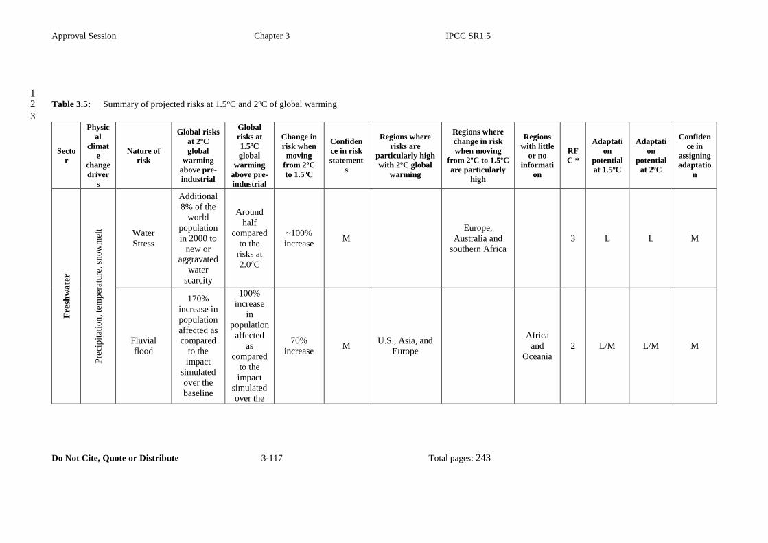
Approval Session Chapter 3 IPCC SR1.5
Do Not Cite, Quote or Distribute 3-117 Total pages: 243
1 Table 3.5: Summary of projected risks at 1.5oC and 2oC of global warming 2
3
Secto
r
Physic
al
climat
e
change
driver
s
Nature of
risk
Global risks
at 2ºC
global
warming
above pre-
industrial
Global
risks at
1.5ºC
global
warming
above pre-
industrial
Change in
risk when
moving
from 2ºC
to 1.5ºC
Confiden
ce in risk
statement
s
Regions where
risks are
particularly high
with 2ºC global
warming
Regions where
change in risk
when moving
from 2ºC to 1.5ºC
are particularly
high
Regions
with little
or no
informati
on
RF
C *
Adaptati
on
potential
at 1.5ºC
Adaptati
on
potential
at 2ºC
Confiden
ce in
assigning
adaptatio
n
Fre
shw
ate
r
Pre
cip
itat
ion
, te
mp
erat
ure
, sn
ow
mel
t
Water
Stress
Additional
8% of the
world
population
in 2000 to
new or
aggravated
water
scarcity
Around
half
compared
to the
risks at
2.0ºC
~100%
increase M
Europe,
Australia and
southern Africa
3 L L M
Fluvial
flood
170%
increase in
population
affected as
compared
to the
impact
simulated
over the
baseline
100%
increase
in
population
affected
as
compared
to the
impact
simulated
over the
70%
increase M
U.S., Asia, and
Europe
Africa
and
Oceania
2 L/M L/M M

Approval Session Chapter 3 IPCC SR1.5
Do Not Cite, Quote or Distribute 3-118 Total pages: 243
Secto
r
Physic
al
climat
e
change
driver
s
Nature of
risk
Global risks
at 2ºC
global
warming
above pre-
industrial
Global
risks at
1.5ºC
global
warming
above pre-
industrial
Change in
risk when
moving
from 2ºC
to 1.5ºC
Confiden
ce in risk
statement
s
Regions where
risks are
particularly high
with 2ºC global
warming
Regions where
change in risk
when moving
from 2ºC to 1.5ºC
are particularly
high
Regions
with little
or no
informati
on
RF
C *
Adaptati
on
potential
at 1.5ºC
Adaptati
on
potential
at 2ºC
Confiden
ce in
assigning
adaptatio
n
period
1976–2005
baseline
period
1976–
2005
Drought
410.7±213.
5 million,
changes in
urban
population
exposure to
severe
drought at
the globe
350.2±15
8.8
million,
changes in
urban
population
exposure
to severe
drought at
the globe
60.5±84.1
million
(±84.1
based on
the SSP1
scenario)
M
Central Europe,
Southern
Europe, the
Mediterranean,
West Africa,
East and West
Asia and
Southeast Asia
2 L/M L/M L
Ter
rest
ria
l
eco
syst
ems
Tem
per
atu
re,
pre
cip
itat
ion
Species
range loss
H (18%
insects, 8%
vertebrates,
16% plants
lose >50%
range)
M (6%
insects,
4%
vertebrate
s, 8%
plants,
lose >50%
range)
Double or
triple H
Amazon,
Europe, South
Africa
1, 4 M L H

Approval Session Chapter 3 IPCC SR1.5
Do Not Cite, Quote or Distribute 3-119 Total pages: 243
Secto
r
Physic
al
climat
e
change
driver
s
Nature of
risk
Global risks
at 2ºC
global
warming
above pre-
industrial
Global
risks at
1.5ºC
global
warming
above pre-
industrial
Change in
risk when
moving
from 2ºC
to 1.5ºC
Confiden
ce in risk
statement
s
Regions where
risks are
particularly high
with 2ºC global
warming
Regions where
change in risk
when moving
from 2ºC to 1.5ºC
are particularly
high
Regions
with little
or no
informati
on
RF
C *
Adaptati
on
potential
at 1.5ºC
Adaptati
on
potential
at 2ºC
Confiden
ce in
assigning
adaptatio
n
Loss of
ecosystem
functioning
and services
H M M
Shifts of
biomes
(major
ecosystem
types)
13% (range
8–20%)
transforme
d
Around
7%
transform
ed
Around
double H
Arctic, Tibet,
Himalayas,
South Africa and
Australia
4 - - -
Hea
t an
d c
old
stre
ss,
war
min
g,
pre
cip
itat
ion
,
dro
ug
ht
Wildfire H H L M Canada, USA,
Mediterranean Mediterranean
Central
and
South
America,
Australia
, Russia,
China,
Africa
1,
2,
4, 5
L L M

Approval Session Chapter 3 IPCC SR1.5
Do Not Cite, Quote or Distribute 3-120 Total pages: 243
Secto
r
Physic
al
climat
e
change
driver
s
Nature of
risk
Global risks
at 2ºC
global
warming
above pre-
industrial
Global
risks at
1.5ºC
global
warming
above pre-
industrial
Change in
risk when
moving
from 2ºC
to 1.5ºC
Confiden
ce in risk
statement
s
Regions where
risks are
particularly high
with 2ºC global
warming
Regions where
change in risk
when moving
from 2ºC to 1.5ºC
are particularly
high
Regions
with little
or no
informati
on
RF
C *
Adaptati
on
potential
at 1.5ºC
Adaptati
on
potential
at 2ºC
Confiden
ce in
assigning
adaptatio
n
Oce
an
War
min
g a
nd
str
atif
icat
ion
of
the
surf
ace
oce
an
Loss of
framework
species
(coral reefs)
very H
(virtually
certain)
H 3 H/very H Tropical/subtrop
ical countries
Tropical/subtrop
ical countries
Southern
Red Sea,
Somalia,
Yemen;
deep
water
coral
reefs
1, 2 H L H
Loss of
framework
species
(seagrass)
H M 5 H/very H Tropical/subtrop
ical countries
Tropical/subtrop
ical countries
Southern
Red Sea,
Somalia,
Yemen;
Myanma
1, 2 M L M/H
Loss of
framework
species
(mangroves)
M/H M 3 M/H Tropical/subtrop
ical countries
Tropical/subtrop
ical countries
Southern
Red Sea,
Somalia,
Yemen;
Myanmar
1, 3 M L M/H
Disruption
of marine
food webs
M L 5 M Global Global Deep Sea 4 M L M/H

Approval Session Chapter 3 IPCC SR1.5
Do Not Cite, Quote or Distribute 3-121 Total pages: 243
Secto
r
Physic
al
climat
e
change
driver
s
Nature of
risk
Global risks
at 2ºC
global
warming
above pre-
industrial
Global
risks at
1.5ºC
global
warming
above pre-
industrial
Change in
risk when
moving
from 2ºC
to 1.5ºC
Confiden
ce in risk
statement
s
Regions where
risks are
particularly high
with 2ºC global
warming
Regions where
change in risk
when moving
from 2ºC to 1.5ºC
are particularly
high
Regions
with little
or no
informati
on
RF
C *
Adaptati
on
potential
at 1.5ºC
Adaptati
on
potential
at 2ºC
Confiden
ce in
assigning
adaptatio
n
Range
migration of
marine
species and
ecosystems
H M 5 H Global Global Deep Sea 1 M L H
Loss of
finfish and
fisheries
M/H M/H 5 H Global Global Deep Sea 4 M M/L M/H
Oce
an a
cid
ific
atio
n a
nd
elev
ated
sea
tem
per
atu
res Loss of
coastal
ecosystems
and
protection
M L/M 5 M
Low latitude
tropical/subtropi
cal countries
Low latitude
tropical/subtropi
cal countries
Most
regions -
risks not
well
defined
1 M M/L M
Loss of
bivalves and
bivalve
fisheries
M M 3 H
Temperate
countries with
up-welling
Temperate
countries with
up-welling
Most
regions -
risks not
well
defined
4 M/H L/M M/H

Approval Session Chapter 3 IPCC SR1.5
Do Not Cite, Quote or Distribute 3-122 Total pages: 243
Secto
r
Physic
al
climat
e
change
driver
s
Nature of
risk
Global risks
at 2ºC
global
warming
above pre-
industrial
Global
risks at
1.5ºC
global
warming
above pre-
industrial
Change in
risk when
moving
from 2ºC
to 1.5ºC
Confiden
ce in risk
statement
s
Regions where
risks are
particularly high
with 2ºC global
warming
Regions where
change in risk
when moving
from 2ºC to 1.5ºC
are particularly
high
Regions
with little
or no
informati
on
RF
C *
Adaptati
on
potential
at 1.5ºC
Adaptati
on
potential
at 2ºC
Confiden
ce in
assigning
adaptatio
n
Changes to
physiology
and ecology
of marine
species
M L/M 3 H Global Global
Most
regions -
risks not
well
defined
4 L L M/H
Red
uce
d b
ulk
oce
an
circ
ula
tio
n a
nd d
e-
ox
yg
enat
ion
.
Increased
hypoxic
dead zones
L/M L 5 L/M
Temperate
countries with
up-welling
Temperate
countries with
up-welling
Deep Sea 4 L L M
Changes to
up-welling
productivity
M L 5 L/M Most upwelling
regions
Most upwelling
regions
Some up-
welling
systems
4 L L M
Inte
ns
ifie
d
sto
rm s,
pre
cip
itat
ion
plu
s
seal
ev
el r
ise Loss of
coastal
ecosystems
H/very H H 5 H Tropical/subtrop
ical countries
Tropical/subtrop
ical countries 1, 4 M L M

Approval Session Chapter 3 IPCC SR1.5
Do Not Cite, Quote or Distribute 3-123 Total pages: 243
Secto
r
Physic
al
climat
e
change
driver
s
Nature of
risk
Global risks
at 2ºC
global
warming
above pre-
industrial
Global
risks at
1.5ºC
global
warming
above pre-
industrial
Change in
risk when
moving
from 2ºC
to 1.5ºC
Confiden
ce in risk
statement
s
Regions where
risks are
particularly high
with 2ºC global
warming
Regions where
change in risk
when moving
from 2ºC to 1.5ºC
are particularly
high
Regions
with little
or no
informati
on
RF
C *
Adaptati
on
potential
at 1.5ºC
Adaptati
on
potential
at 2ºC
Confiden
ce in
assigning
adaptatio
n
Inundation
and
destruction
of
human/coast
al
infrastructur
e and
livelhoods.
H/very H H 5 H Global Global 1, 5 M/H M M/L
Lo
ss o
f se
a ic
e
Loss of
habitat very H H 5 H Polar regions Polar regions 1 L very L H
Increased
productivity
but
changing
fisheries
M/H L/M 5 very H Polar regions Polar regions 1, 4 L M/L H
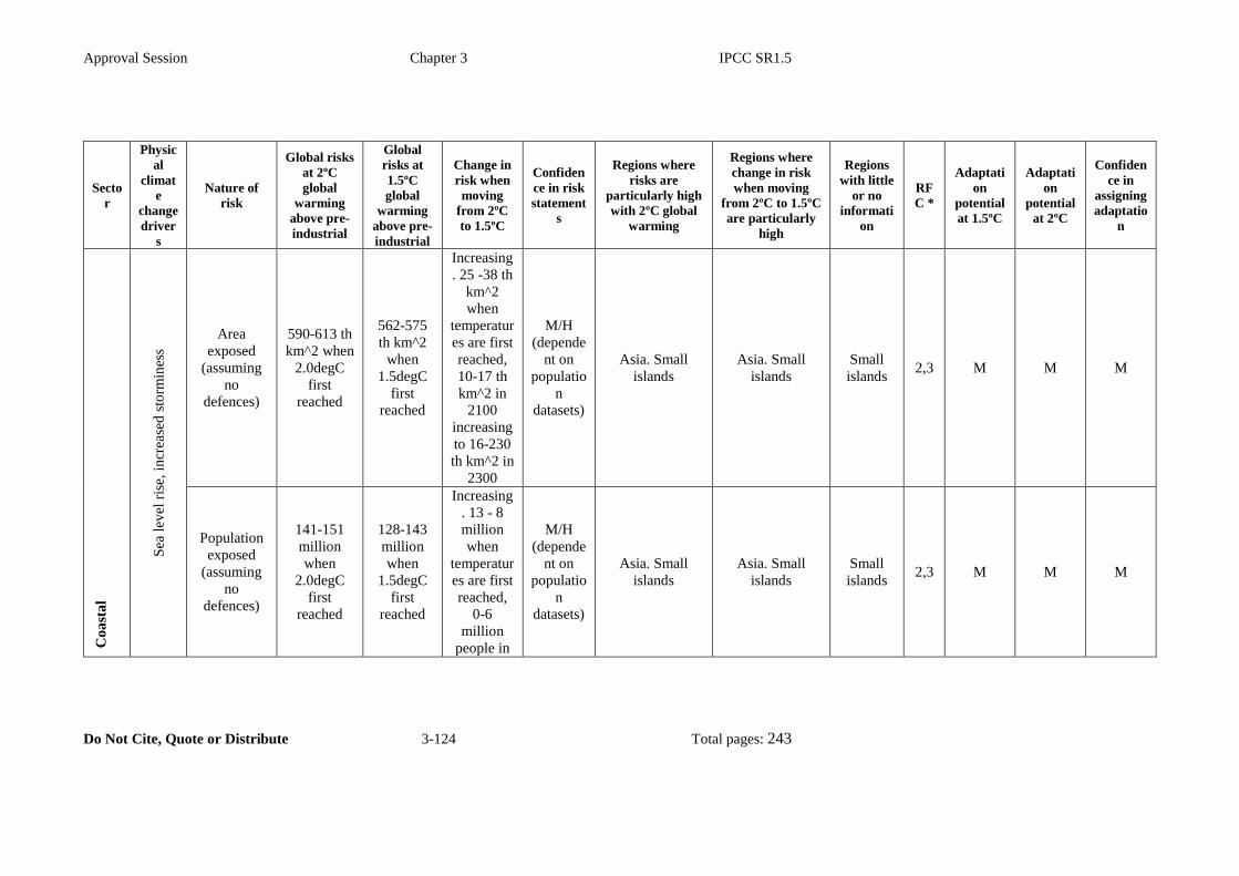
Approval Session Chapter 3 IPCC SR1.5
Do Not Cite, Quote or Distribute 3-124 Total pages: 243
Secto
r
Physic
al
climat
e
change
driver
s
Nature of
risk
Global risks
at 2ºC
global
warming
above pre-
industrial
Global
risks at
1.5ºC
global
warming
above pre-
industrial
Change in
risk when
moving
from 2ºC
to 1.5ºC
Confiden
ce in risk
statement
s
Regions where
risks are
particularly high
with 2ºC global
warming
Regions where
change in risk
when moving
from 2ºC to 1.5ºC
are particularly
high
Regions
with little
or no
informati
on
RF
C *
Adaptati
on
potential
at 1.5ºC
Adaptati
on
potential
at 2ºC
Confiden
ce in
assigning
adaptatio
n
Co
ast
al
Sea
lev
el r
ise,
in
crea
sed
sto
rmin
ess
Area
exposed
(assuming
no
defences)
590-613 th
km^2 when
2.0degC
first
reached
562-575
th km^2
when
1.5degC
first
reached
Increasing
. 25 -38 th
km^2
when
temperatur
es are first
reached,
10-17 th
km^2 in
2100
increasing
to 16-230
th km^2 in
2300
M/H
(depende
nt on
populatio
n
datasets)
Asia. Small
islands
Asia. Small
islands
Small
islands 2,3 M M M
Population
exposed
(assuming
no
defences)
141-151
million
when
2.0degC
first
reached
128-143
million
when
1.5degC
first
reached
Increasing
. 13 - 8
million
when
temperatur
es are first
reached,
0-6
million
people in
M/H
(depende
nt on
populatio
n
datasets)
Asia. Small
islands
Asia. Small
islands
Small
islands 2,3 M M M

Approval Session Chapter 3 IPCC SR1.5
Do Not Cite, Quote or Distribute 3-125 Total pages: 243
Secto
r
Physic
al
climat
e
change
driver
s
Nature of
risk
Global risks
at 2ºC
global
warming
above pre-
industrial
Global
risks at
1.5ºC
global
warming
above pre-
industrial
Change in
risk when
moving
from 2ºC
to 1.5ºC
Confiden
ce in risk
statement
s
Regions where
risks are
particularly high
with 2ºC global
warming
Regions where
change in risk
when moving
from 2ºC to 1.5ºC
are particularly
high
Regions
with little
or no
informati
on
RF
C *
Adaptati
on
potential
at 1.5ºC
Adaptati
on
potential
at 2ºC
Confiden
ce in
assigning
adaptatio
n
2100,
increasing
to 35-95
million
people in
2300
People at
risk taking
account of
defences
(modelled
in 1995)
Between
14.9-52.3
million
people / yr
if defences
are not
upgraded
from the
modelled
1995
baseline
Between
2.3-27.8
million
people / yr
as
defences
are not
upgraded
from the
1995
baseline
Increasing
with time,
but highly
dependent
on
adaptation
.
M/H
(depende
nt on
adaptatio
n)
Asia. Small
islands.
Potentially
African nations.
Asia. Small
islands
Small
islands
2,3,
4 M M M

Approval Session Chapter 3 IPCC SR1.5
Do Not Cite, Quote or Distribute 3-126 Total pages: 243
Secto
r
Physic
al
climat
e
change
driver
s
Nature of
risk
Global risks
at 2ºC
global
warming
above pre-
industrial
Global
risks at
1.5ºC
global
warming
above pre-
industrial
Change in
risk when
moving
from 2ºC
to 1.5ºC
Confiden
ce in risk
statement
s
Regions where
risks are
particularly high
with 2ºC global
warming
Regions where
change in risk
when moving
from 2ºC to 1.5ºC
are particularly
high
Regions
with little
or no
informati
on
RF
C *
Adaptati
on
potential
at 1.5ºC
Adaptati
on
potential
at 2ºC
Confiden
ce in
assigning
adaptatio
n
Fo
od
sec
uri
ty a
nd
fo
od
pro
du
ctio
n
syst
ems
Hea
t an
d c
old
stre
ss,
war
min
g,
pre
cip
itat
ion
,
dro
ug
ht
Changes in
ecosystem
production
H M/H M/H M/H Global
Noth America,
Central and
South America,
Mediterranean
basin, South
Africa,
Australia, Asia
- - - 2,
4,5 H M/H M/H
Hea
t an
d c
old
stre
ss,
war
min
g,
pre
cip
itat
ion
,
dro
ug
ht
Shift and
composition
change of
biomes
(major
ecosystem
types)
H M/H M L/M Global
Global, Tropical
areas,
Mediterranean
Africa,
Asia
1,
2,
3, 4
L/M L L/M
Hu
ma
n h
ealt
h
Tem
per
atu
re
Heat-related
morbidity
and
mortality
M/H M Risk
increased VH
All regions at
risk All regions Africa
2,3,
4 H H H
Occupationa
l heat stress M/H M
Risk
increased M Tropical regions Tropical regions Africa
2,3,
4 H M M

Approval Session Chapter 3 IPCC SR1.5
Do Not Cite, Quote or Distribute 3-127 Total pages: 243
Secto
r
Physic
al
climat
e
change
driver
s
Nature of
risk
Global risks
at 2ºC
global
warming
above pre-
industrial
Global
risks at
1.5ºC
global
warming
above pre-
industrial
Change in
risk when
moving
from 2ºC
to 1.5ºC
Confiden
ce in risk
statement
s
Regions where
risks are
particularly high
with 2ºC global
warming
Regions where
change in risk
when moving
from 2ºC to 1.5ºC
are particularly
high
Regions
with little
or no
informati
on
RF
C *
Adaptati
on
potential
at 1.5ºC
Adaptati
on
potential
at 2ºC
Confiden
ce in
assigning
adaptatio
n
Air
qu
alit
y
Ozone-
related
mortality
M/H (if
precursor
emissions
remain the
same)
M (if
precursor
emissions
remain the
same)
Risk
increased H
High income and
emerging
economies
High income and
emerging
economies
Africa,
parts of
Asia
2,3,
4 L L M
Tem
per
atu
re,
pre
cip
itat
i
on Undernutriti
on M/H M
Risk
increased H
Low-income
countries in
Africa and Asia
Low-income
countries in
Africa and Asia
Small
islands
2,3,
4 M L M
Key
eco
no
mic
secto
rs
Tem
per
atu
re
Tourism
(sun and
beach, and
snow
sports)
H M/H Risk
increased VH
Coastal tourism,
particularly in
sub-tropical and
tropical regions
Coastal tourism,
particularly in
sub-tropical and
tropical regions
Africa 1,2,
3 M L H
*RFC: 1 = unique and threatened systems, 2 = extreme events, 3 = unequal distribution of impacts, 4 = global aggregate impacts (economic + biodiversity), 5 = large scale 1 singular events 2
3
4
5
6

Approval Session Chapter 3 IPCC SR1.5
Do Not Cite, Quote or Distribute 3-128 Total pages: 243
3.4.13 Synthesis of key elements of risk 1
2 Some elements of the assessment in Section 3.4 are synthesised in a single diagram (Figure 3.19) that 3
indicates the overall risk in five broad categories for natural and human systems as a result of anthropogenic 4
climate change and increases in Global Mean Surface Temperature (GMST). The elements included are 5
supported by a substantive enough body of literature providing at least medium confidence in the assessment. 6
The format for figure 3.19 matches that of Figure 19.4 of WGII AR5 Chapter 19 (Oppenheimer et al., 2014) 7
and Figure 3.19) by indicating the levels of the transition of risk from undetectable to moderate (detected and 8
attributed), from moderate to high (severe and widespread) and from high to very high, the latter indicating 9
significant irreversibility or persistence of climate-related hazards combined with a much reduced capacity to 10
adapt. Regarding the transition from undetectable to moderate, the impact literature assessed in the AR5 11
focused on describing and quantifying linkages between weather and climate patterns and impact outcomes, 12
with limited detection and attribution to anthropogenic climate change (Cramer et al., 2014). A more recent 13
analysis of attribution to greenhouse gas forcing at the global scale (Hansen and Stone, 2016) confirmed that 14
the impacts related to changes in regional atmospheric and ocean temperature can be confidently attributed 15
to anthropogenic forcing, while attribution to anthropogenic forcing of those related to precipitation is only 16
weakly evident or absent. Moreover, there is no strong direct relationship between the robustness of climate 17
attribution and that of impact attribution (Hansen and Stone, 2016). 18
19 The current synthesis is complementary to the synthesis in Section 3.5.2 that categorizes risks into ‘Reasons 20
for Concern’ (RFCs), as described in Oppenheimer et al. (2014). Each element presented here maps to one or 21
more RFCs, and the figure indicates this relationship. It should be emphasized that risks to the issues 22
assessed here are only a subset of the full range of risks that contribute to the RFCs. This figure is not 23
intended to replace the RFCs but rather to indicate how risks to particular elements of the earth system 24
accrue with global warming, with a focus on levels of warming of 1.5°C and 2°C. Key evidence assessed in 25
earlier parts of this chapter are summarized to indicate the transition points between the levels of risk. A 26
fuller account is in the Supplemantary Material 3.SM S3-4-12. 27
28
In terrestrial ecosystems (related to RFC1 and RFC4), detection and attribution studies show that impacts of 29
climate change on terrestrial ecosystems began to take place over the few decades, indicating a transition 30
from no risk (white ) to moderate risk (yellow) below recent temperatures (high confidence, Section 3.4.3). 31
Risks to unique and threatened terrestrial ecosystems are generally higher under warming of 2°C as 32
compared to 1.5°C (Section 3.5.2.1), while at the global scale, severe and widespread risks (red) are 33
projected to occur by 2°C of warming. These risks are associated with biome shifts and species range loss 34
(Sections 3.4.3 and 3.5.2.4); however, because many systems and species are unable to adapt to levels of 35
warming below 2°C, the transition to high risk (red) is located below 2°C (high confidence). At 3°C of 36
warming, however, biome shifts and species range losses escalate to very high levels and the systems have 37
very little capacity to adapt (purple; Section 3.4.3; high confidence). 38
39
In the Arctic (related to RFC1), the increased rate of summer sea ice melt was detected and attributed to 40
climate change by the year 2000 (corresponding to warming of 0.7°C), indicating moderate risk (yellow). At 41
1.5°C warming, an ice-free Arctic ocean is considered unlikely whilst by 2°C warming it is considered likely 42
and this unique ecosystem is considered unable to adapt, hence a transition from high (red) to very high 43
(purple) risk is expected between 1.5°C and 2°C warming. 44
45
For coral reefs, there is high confidence in the transitions between colour assignments, especially in the 46
growing impacts in the transition of warming from 0.4°C to 0.6°C, and in projections of change from 0.6ºC to 47
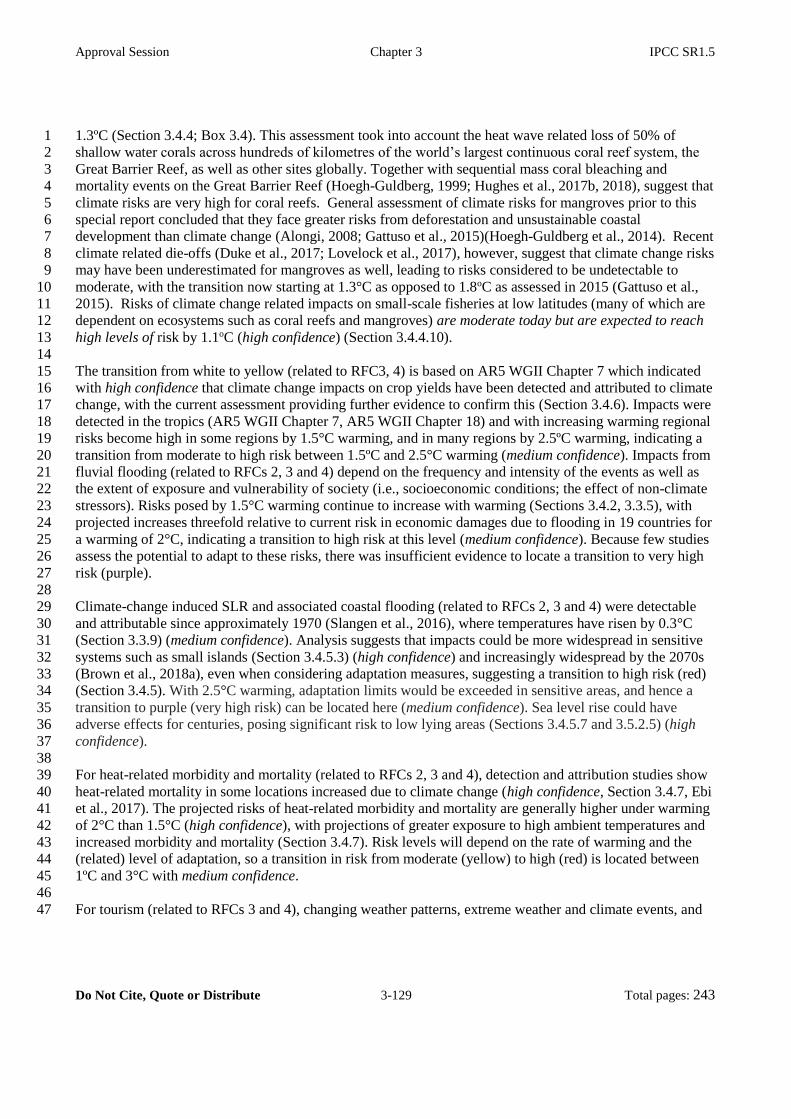
Approval Session Chapter 3 IPCC SR1.5
Do Not Cite, Quote or Distribute 3-129 Total pages: 243
1.3ºC (Section 3.4.4; Box 3.4). This assessment took into account the heat wave related loss of 50% of 1
shallow water corals across hundreds of kilometres of the world’s largest continuous coral reef system, the 2
Great Barrier Reef, as well as other sites globally. Together with sequential mass coral bleaching and 3
mortality events on the Great Barrier Reef (Hoegh-Guldberg, 1999; Hughes et al., 2017b, 2018), suggest that 4
climate risks are very high for coral reefs. General assessment of climate risks for mangroves prior to this 5
special report concluded that they face greater risks from deforestation and unsustainable coastal 6
development than climate change (Alongi, 2008; Gattuso et al., 2015)(Hoegh-Guldberg et al., 2014). Recent 7
climate related die-offs (Duke et al., 2017; Lovelock et al., 2017), however, suggest that climate change risks 8
may have been underestimated for mangroves as well, leading to risks considered to be undetectable to 9
moderate, with the transition now starting at 1.3°C as opposed to 1.8oC as assessed in 2015 (Gattuso et al., 10
2015). Risks of climate change related impacts on small-scale fisheries at low latitudes (many of which are 11
dependent on ecosystems such as coral reefs and mangroves) are moderate today but are expected to reach 12
high levels of risk by 1.1oC (high confidence) (Section 3.4.4.10). 13
14
The transition from white to yellow (related to RFC3, 4) is based on AR5 WGII Chapter 7 which indicated 15
with high confidence that climate change impacts on crop yields have been detected and attributed to climate 16
change, with the current assessment providing further evidence to confirm this (Section 3.4.6). Impacts were 17
detected in the tropics (AR5 WGII Chapter 7, AR5 WGII Chapter 18) and with increasing warming regional 18
risks become high in some regions by 1.5°C warming, and in many regions by 2.5ºC warming, indicating a 19
transition from moderate to high risk between 1.5ºC and 2.5°C warming (medium confidence). Impacts from 20
fluvial flooding (related to RFCs 2, 3 and 4) depend on the frequency and intensity of the events as well as 21
the extent of exposure and vulnerability of society (i.e., socioeconomic conditions; the effect of non-climate 22
stressors). Risks posed by 1.5°C warming continue to increase with warming (Sections 3.4.2, 3.3.5), with 23
projected increases threefold relative to current risk in economic damages due to flooding in 19 countries for 24
a warming of 2°C, indicating a transition to high risk at this level (medium confidence). Because few studies 25
assess the potential to adapt to these risks, there was insufficient evidence to locate a transition to very high 26
risk (purple). 27
28
Climate-change induced SLR and associated coastal flooding (related to RFCs 2, 3 and 4) were detectable 29
and attributable since approximately 1970 (Slangen et al., 2016), where temperatures have risen by 0.3°C 30
(Section 3.3.9) (medium confidence). Analysis suggests that impacts could be more widespread in sensitive 31
systems such as small islands (Section 3.4.5.3) (high confidence) and increasingly widespread by the 2070s 32
(Brown et al., 2018a), even when considering adaptation measures, suggesting a transition to high risk (red) 33
(Section 3.4.5). With 2.5°C warming, adaptation limits would be exceeded in sensitive areas, and hence a 34
transition to purple (very high risk) can be located here (medium confidence). Sea level rise could have 35
adverse effects for centuries, posing significant risk to low lying areas (Sections 3.4.5.7 and 3.5.2.5) (high 36
confidence). 37
38
For heat-related morbidity and mortality (related to RFCs 2, 3 and 4), detection and attribution studies show 39
heat-related mortality in some locations increased due to climate change (high confidence, Section 3.4.7, Ebi 40
et al., 2017). The projected risks of heat-related morbidity and mortality are generally higher under warming 41
of 2°C than 1.5°C (high confidence), with projections of greater exposure to high ambient temperatures and 42
increased morbidity and mortality (Section 3.4.7). Risk levels will depend on the rate of warming and the 43
(related) level of adaptation, so a transition in risk from moderate (yellow) to high (red) is located between 44
1ºC and 3°C with medium confidence. 45
46
For tourism (related to RFCs 3 and 4), changing weather patterns, extreme weather and climate events, and 47

Approval Session Chapter 3 IPCC SR1.5
Do Not Cite, Quote or Distribute 3-130 Total pages: 243
sea level rise are affecting many (but not all) global tourism investments and environmental and cultural 1
destination assets (Section 3.4.4.12), with ‘last chance’ tourism markets developing based on observed 2
impacts on environmental and cultural heritage (Section 3.4.9.1), indicating a transition from undetected to 3
moderate risk between 0°C and 1.5°C (high confidence). Based on limited analyses, risks to the tourism 4
sector are higher at 2°C than at 1.5°C, with greater impacts on climate-sensitive sun, beach, and snow sports 5
tourism markets. The degradation or loss of coral reef systems will increase the risks to coastal tourism, 6
particularly in sub-tropical and tropical regions. A transition in risk from moderate (yellow) to high (red) is 7
located between 1.5 and 3°C (medium confidence). 8
9
Owing to the existing effects that climate change is already having upon ecosystems, human health and 10
agriculture, climate change is already beginning to make it more difficult to reach goals to eradicate poverty 11
and hunger and protect health and life on land (Sections 5.1 and 5.2.1), suggesting a transition from 12
undetected to moderate risk below recent temperatures at 0.5°C warming (medium confidence). Based 13
on limited analyses there is evidence and agreement that the risks to sustainable development are 14
considerably less at 1.5°C than 2°C (Section 5.2.2) including avoided impacts on poverty and food security. 15
It is easier to achieve many of the Sustainable Development Goals (SDGs) at 1.5°C, suggesting that a 16
transition to higher risk has not yet begin at this level. At 2°C and higher (e.g., RCP8.5) however, there are 17
high risks of failure to meet SDGs such as eradicating poverty and hunger, providing safe water, 18
reducing inequality, and protecting ecosystems and which are likely to become severe and widespread if 19
warming were increase further to about 3°C (medium confidence) (Section 5.2.3). 20
21
Disclosure statement: The selection of elements is not intended to be fully comprehensive and does not 22
necessarily include all elements for which there is a substantive body of literature, nor does it necessarily 23
include all elements which are of particular interest to decision makers. 24
25
26
27
28

Approval Session Chapter 3 IPCC SR1.5
Do Not Cite, Quote or Distribute 3-131 Total pages: 243
1 Figure 3.20: The dependence of risk associated with selected elements of human and natural systems on the level of 2
climate change, adapted from Figure 3.18 and from AR5 WGII Chapter 19, and highlighting the nature of 3 this dependence between 0 and 2ºC warming above pre-industrial levels. The color scheme indicates the 4 additional risks due to climate change. The shading of each ember provides a qualitative indication of the 5 increase in risk with temperature for each individual ‘element’. At one end, undetectable risk (white) 6 indicates no detection and attribution of climate change with at least medium confidence. At the other end 7 of the risk spectrum, the transition from red to purple, introduced for the first time in AR4, is defined by 8 very high risk and the presence of significant irreversibility or persistence of climate-related hazards 9 combined with limited ability to adapt due to the nature of the hazard or impact. Comparison of the 10 increase of risk across elements indicates the relative sensitivity of elements to increases in Global Mean 11 Surface Temperature (GMST). As was done previously, this assessment takes autonomous adaptation into 12 account, as well as limits to adaptation independently of development pathway. The levels of risk 13 illustrated reflect the judgements of the authors of Chapter 3 and Gattuso et al. (2015; for three marine 14 elements). 15
16
17
18
Avoided impacts and reduced risks at 1.5ºC compared with 2ºC 19
20
3.5.1 Introduction 21
22
Oppenheimer et al. (2014, AR5 Chapter 19) provide a framework that aggregates projected risks from global 23

Approval Session Chapter 3 IPCC SR1.5
Do Not Cite, Quote or Distribute 3-132 Total pages: 243
mean temperature change into five categories known as ‘Reasons for Concern’. Risks are classified as 1
moderate, high, or very high and coloured yellow, red and purple respectively in Figure 19.4 (see AR5 2
Chapter 19 for details and findings). The framework’s conceptual basis and the risk judgments made in 3
Oppenheimer et al. (2014) were recently reviewed, confirming most judgements made in the light of more 4
recent literature (O’Neill et al., 2017). We adopt the approach of Oppenheimer et al. (2014), with updates in 5
terms of the aggregation of risk as informed by the most recent literature, for the analysis of avoided impacts 6
at 1.5°C compared to 2°C of global warming presented in this section. 7
8
The economic benefits to be obtained by achieving the global temperature goal of 1.5°C, as compared to 2°C 9
(or higher) are discussed in Section 3.5.3 in the light of the five reasons for concern explored in Section 10
3.5.2. Climate change hot spots that can be avoided or reduced by achieving the 1.5°C target are summarised 11
in Section 3.5.4. The section concludes with a discussion of regional tipping points that can be avoided at 12
1.5ºC compared to higher degrees of global warming (Section 3.5.5). 13
14
15
3.5.2 Aggregated avoided impacts and reduced risks at 1.5°C versus 2°C of global warming 16
17
A brief summary of the accrual of RFC with global warming as assessed in WGII AR5 is provided in the 18
following sections, which leads into an update of relevant literature published since AR5. The new literature 19
is used to confirm the levels of global warming at which risks are considered to increase to moderate, and 20
from moderate to high, and from high to very high. Figure 3.20 modifies Figure 19.4 from AR5 WGII with 21
the ensuing text in this subsection providing the justification for the modifications. O'Neill et al. (2017) 22
presents a very similar assessment to WGII AR%, but with further discussion of the future potential to create 23
socioeconomic-scenario specific embers. At present, there is insufficient literature to do this so the original 24
simple approach has been used here. Since the focus in the present assessment is on the conseqeunces of 25
warming of 1.5ºC to 2°C, with no assessment for global warming of 3°C or more are not included, the 26
embers developed here are discontinued at 3ºC. 27
28
29

Approval Session Chapter 3 IPCC SR1.5
Do Not Cite, Quote or Distribute 3-133 Total pages: 243
Figure 3.21: The dependence of risk associated with the Reasons for Concern (RFCs) on the level of climate change, 1 updated and adapted from WGII AR5 Ch 19, Figure 19.4 and highlighting the nature of this dependence 2 between 0ºC and 2ºC warming above pre-industrial levels. The color scheme indicates the additional risks 3 due to climate change. The shading of each ember provides a qualitative indication of the increase in risk 4 with temperature for each individual ‘reason’. The transition from red to purple, introduced for the first 5 time in AR4, is defined by very high risk and the presence of significant irreversibility or persistence of 6 climate-related hazards combined with limited ability to adapt due to the nature of the hazard or impact. 7 Comparison of the increase of risk across RFCs indicates the relative sensitivity of RFCs to increases in 8 GMST. As was done previously, this assessment takes autonomous adaptation into account, as well as 9 limits to adaptation (RFC 1, 3, 5) independently of development pathway. The rate and timing of impacts 10 were taken into account in assessing RFC 1 and 5. The levels of risk illustrated reflect the judgements of 11 the Ch 3 authors. [Note to reviewers: In WGII AR5 Ch 19 and more recently in O’Neill et al. 2017 the 12 need to detail how these kinds of figures vary with socioeconomic pathway is noted and suggestions are 13 made therein as to how this might be done. That is seen as a task for IPCC AR6, and beyond the scope of 14 what is feasible to do for SR1.5] 15
16
17
18
RFC 1- Unique and threatened systems 19
WGII AR5 Chapter 19 found that some unique and threatened systems are at risk from climate change at 20
current temperatures, with increasing numbers of systems at risk of severe consequences at global warming 21
of 1.6ºC above pre-industrial levels. It was also observed that many species and ecosystems have limited 22
ability to adapt to the very large risks associated with warming of 2.6ºC or more, particularly Arctic sea ice 23
and coral reef systems (high confidence). A transition from white to yellow indicating the onset of moderate 24
risk was therefore located below present day global temperatures (medium confidence); a transition from 25
yellow to red indicating the onset of high risk was located at 1.6ºC, and a transition to purple indicating the 26
onset of very high risk at about 2.6ºC. This WGII AR5 analysis already implies a significant reduction in 27
risks to unique and threatened systems if warming is limited to 1.5ºC as compared with 2ºC. Since AR5, 28
evidence of present day impacts in these systems has continued to grow (Sections 3.4.2.2, 3.4.2.3, and 29
3.4.2.5), whilst new evidence has also accumulated about increased risks at 1.5ºC vs 2°C warming in Arctic 30
ecosystems (Section 3.3.9), coral reefs (Section 3.4.3), some other unique ecosystems (Section 3.4.2) and 31
biodiversity. 32
33
New literature since AR5 provides a closer focus on the comparative levels of risk to coral reefs at 1.5ºC 34
versus 2ºC global warming. As assessed in Section 3.4.4 and Box 3.4, reaching 2ºC will increase the 35
frequency of mass coral bleaching and mortality to a point at which it will result in the total loss of coral 36
reefs from the world’s tropical and subtropical regions. Restricting overall warming to 1.5ºC will still see a 37
downward trend in average coral cover (70–90% decline by mid-century) but will prevent the total loss of 38
coral reefs projected with warming of 2°C. The remaining reefs at 1.5°C will also benefit from increasingly 39
stable ocean conditions by the mid-to-late 21st century. Limiting global warming to 1.5°C during the course 40
of the century may, therefore, open the window for many ecosystems to adapt or reassort geographically past 41
climate change. This indicates a transition in risk in this system from high to very high (red to purple) (high 42
confidence) at 1.5ºC warming and contributes to a lowering of the transition from high to very high (red to 43
purple) in this RFC1 compared to AR5. Further details of risk transitions for ocean systems are described in 44
Figure 3.20. 45
46
Substantial losses of Arctic Ocean summer ice were projected in AR5 WGI for global warming of 1.6ºC, 47
with a nearly ice-free Arctic Ocean being projected for global warming of greater than 2.6ºC. Since AR5, the 48

Approval Session Chapter 3 IPCC SR1.5
Do Not Cite, Quote or Distribute 3-134 Total pages: 243
importance of a threshold between 1ºC and 2ºC has been further emphasized in the literature, with sea ice 1
projected to persist throughout the year for a global warming less than 1.5ºC, yet chances of an ice-free 2
Arctic during summer being high at 2°C warming (Section 3.3.8). Less of the permafrost in the Arctic is 3
projected to thaw (21–37% under 1.5ºC warming as compared with 35–47% for 2ºC warming) (Section 4
3.3.5.2), which would be expected to reduce risks to both social and ecological systems in the Arctic. This 5
indicates a transition in risk in this system from high to very high (red to purple) between 1.5ºC and 2ºC 6
warming and contributes to a lowering of the transition from high to very high (red to purple) in this RFC1 7
compared to AR5. 8
9
AR5 identifies a large number of threatened systems including mountain ecosystems, highly biodiverse 10
tropical wet and dry forests, deserts, freshwater systems and dune systems. These include the Mediterranean 11
areas in Europe, Siberian, tropical and desert ecosystems in Asia, Australian rainforests, the Fynbos and 12
succuluent Karoo areas of S. Africa, and wetlands in Ethiopia, Malawi, Zambia and Zimbabwe. In all these 13
systems, impacts accrue with greater warming and impacts at 2ºC being expected to be greater than those at 14
1.5ºC (medium confidence). One study since the AR5 has shown that constraining global warming to 1.5ºC 15
would maintain the functioning of the prairie pothole ecosystem (north America) in terms of its productivity 16
and biodiversity, whilst a warming of 2ºC would not do so (Carter Johnson et al., 2016). The large 17
proportion of insects projected to lose over half their range at 2ºC warming (25%) as compared to 1.5°C 18
warming (9%) also suggests a significant loss of functionality in these systems at 2ºC warming owing to the 19
key role of insects in nutrient cycling, pollination, detritivory, and other key ecosystem processes (Section 20
3.4.2). 21
22
Unique and threatened systems in small island states and in systems fed by glacier meltwater were also 23
considered in AR5 in making a contribution to this RFC, but there is little new information about these systems 24
that pertains to 1.5ºor 2ºC global warming. 25
26
Taken together, the evidence suggests that the transition from high to very high risk (red to purple) in unique 27
and threatened systems occurs at a lower level of warming, between 1.5ºC and 2ºC (high confidence), than in 28
AR5 where this transition was located at 2.6ºC. The transition from moderate to high risk (yellow to red) 29
would relocate very slightly from 1.6ºC to 1.5ºC. 30
31
RFC 2- Extreme weather events 32
In this sub-subsection reduced risks in terms of the likelihood of occurrence of extreme weather events are 33
discussed for 1.5ºC as compared to 2ºC of global warming – for those extreme events where current evidence 34
is available. AR5 assigned a moderate (yellow) level of risk due to extreme weather events at recent 35
temperatures (1986-2005) due to the attribution of heat and precipitation extremes to climate change, and a 36
transition to high (red) beginning below 1.6ºC global warming based on the magnitude, likelihood and 37
timing of projected changes in risk associated with extreme events, indicating more severe and widespread 38
impacts. The AR5 analysis already suggests a significant benefit of limiting warming to 1.5ºC, since this 39
might keep risks closer to the moderate level. New literature since AR5 provides greater confidence in a 40
reduced level of risks due to extreme weather events at 1.5ºC versus 2ºC for some types of extremes (see 41
Section 3.3 and below). 42
43

Approval Session Chapter 3 IPCC SR1.5
Do Not Cite, Quote or Distribute 3-135 Total pages: 243
Temperature: It is very likely that further increases in number of warm days/nights and decrease in number 1
of cold days/nights and in overall temperature of hot and cold extremes will occur under 1.5ºC of global 2
warming compared to present-day climate (1°C warming), with further increases towards 2ºC of warming 3
(section 3.3). As assessed in Sections 3.3.1 and 3.3.2, impacts of a 0.5°C global warming can be identified 4
for temperature extremes at global scales, based on observations and the analysis of climate models. At 2ºC 5
of global warming, it is likely that temperature increases of more than 2°C will occur over most land regions 6
in terms of extreme temperatures (on average between 3 and 8°C depending on region and considered 7
extreme index) (Section 3.3.2). Regional increases in temperature extremes under 1.5°C of global warming, 8
can be reduced to 2–6°C (Section 3.3.2). Benefits to be obtained from this general reduction in extremes 9
depends to a large extent on whether the lower range of increases in extremes at 1.5ºC is sufficient for 10
critical thresholds to be exceeded, within the context of wide-ranging aspects such as crop yields, human 11
health and the sustainability of ecosystems. 12
13
Heavy precipitation: AR5 assessed trends in heavy precipitation for land regions where observational 14
coverage was sufficient for assessment. It concluded with medium confidence that anthropogenic forcing has 15
contributed to a global-scale intensification of heavy precipitation over the second half of the 20th century. A 16
recent observations-based study also shows that a 0.5°C increase in global mean temperature has a detectable 17
effect on changes in precipitation extremes at global scale (Schleussner et al., 2017), thus suggesting that 18
there would be detectable differences in heavy precipitation at 1.5°C and 2°C of global warming. These 19
results are consistent with analyses of climate projections, although they also highlight a large amount of 20
regional variation in the sensitivity of changes in heavy precipitation (Section 3.3.3). 21
22
Droughts: When considering the difference between precipitation minus evaporation as a function of global 23
temperature changes, the subtropics generally display an overall trend towards drying, whilst the northern 24
high latitudes display a robust response towards increased wetting (Section 3.3.4, Figure 3.12). Limiting 25
global mean temperature increase to 1.5°C as opposed to 2°C could substantially reduce the risk of reduced 26
regional water availability (Section 3.3.4). Regions that are to benefit include much of South America, 27
southern Africa, Australia and the Mediterranean. 28
29
Fire: The increased amount of evidence that anthropogenic climate change has already caused significant 30
increases in fire area globally (Section 3.4.3) is in line with projected fire risks. These risks are projected to 31
increase further under 1.5ºC of global warming relative to the present day (Section 3.4.3). Under 1.2°C of 32
global warming, fire frequency was estimated to increase by over 37.8% of global land areas, compared to 33
61.9% of global land areas under 3.5°C of warming. For in-depth discussion and uncertainty estimates, see 34
(Meehl et al., 2007; Moritz et al., 2012; Romero-Lankao et al., 2014). 35
36
In “Extreme Weather Events” (RFC2) the transition from moderate to high risk is located between 1oC and 37
1.5oC global warming, which is very similar to the AR5 assessment but there is greater confidence in the 38
assessment (medium confidence). The impact literature contains little information about the potential for 39
human society to adapt to extreme weather events and hence it has not been possible to locate the transition 40
from 'high' (red) to 'very high' risk within the context of assessing impacts at 1.5°C vs 2°C global warming. 41
There is thus low confidence in the level at which global warming could lead to very high risks associated 42
with extreme weather events in the context of this report. 43
44
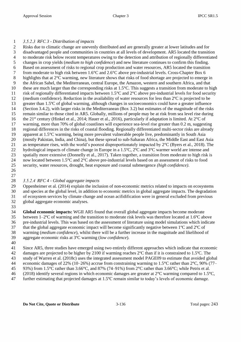
Approval Session Chapter 3 IPCC SR1.5
Do Not Cite, Quote or Distribute 3-136 Total pages: 243
RFC 3 - Distribution of impacts 1
Risks due to climatic change are unevenly distributed and are generally greater at lower latitudes and for 2
disadvantaged people and communities in countries at all levels of development. AR5 located the transition 3
to moderate risk below recent temperatures owing to the detection and attribution of regionally differentiated 4
changes in crop yields (medium to high confidence) and new literature continues to confirm this finding. 5
Based on assessment of risks to regional crop production and water resources, AR5 located the transition 6
from moderate to high risk between 1.6°C and 2.6°C above pre-industrial levels. Cross-Chapter Box 6 7
highlights that at 2°C warming, new literature shows that risks of food shortage are projected to emerge in 8
the African Sahel, the Mediterranean, central Europe, the Amazon, western and southern Africa, and that 9
these are much larger than the corresponding risks at 1.5°C. This suggests a transition from moderate to high 10
risk of regionally differentiated impacts between 1.5°C and 2°C above pre-industrial levels for food security 11
(medium confidence). Reduction in the availability of water resources for less than 2ºC is projected to be 12
greater than 1.5ºC of global warming, although changes in socioeconomics could have a greater influence 13
(Section 3.4.2), with larger risks in the Mediterranean (Box 3.2) but estimates of the magnitude of the risks 14
remain similar to those cited in AR5. Globally, millions of people may be at risk from sea level rise during 15
the 21st century (Hinkel et al., 2014; Hauer et al., 2016), particularly if adaptation is limited. At 2°C of 16
warming, more than 70% of global coastlines will experience sea-level rise greater than 0.2 m, suggesting 17
regional differences in the risks of coastal flooding. Regionally differentiated multi-sector risks are already 18
apparent at 1.5°C warming, being more prevalent vulnerable people live, predominantly in South Asia 19
(mostly Pakistan, India, and China), but these spread to sub-Saharan Africa, the Middle East and East Asia 20
as temperature rises, with the world’s poorest disproportionately impacted by 2°C (Byers et al., 2018). The 21
hydrological impacts of climate change in Europe in a 1.5ºC, 2ºC and 3°C warmer world are intense and 22
spatially more extensive (Donnelly et al., 2017). Taken together, a transition from moderate to high risk is 23
now located between 1.5°C and 2°C above pre-industrial levels based on an assessment of risks to food 24
security, water resources, drought, heat exposure and coastal submergence (high confidence). 25
26
27
RFC 4 - Global aggregate impacts 28
Oppenheimer et al. (2014) explain the inclusion of non-economic metrics related to impacts on ecosystems 29
and species at the global level, in addition to economic metrics in global aggregate impacts. The degradation 30
of ecosystem services by climate change and ocean acifidification were in general excluded from previous 31
global aggregate economic analyses. 32
33
Global economic impacts: WGII AR5 found that overall global aggregate impacts become moderate 34
between 1–2ºC of warming and the transition to moderate risk levels was therefore located at 1.6ºC above 35
pre-industrial levels. This was based on the assessment of literature using model simulations which indicate 36
that the global aggregate economic impact will become significantly negative between 1ºC and 2ºC of 37
warming (medium confidence), whilst there will be a further increase in the magnitude and likelihood of 38
aggregate economic risks at 3ºC warming (low confidence). 39
40
Since AR5, three studies have emerged using two entirely different approaches which indicate that economic 41
damages are projected to be higher by 2100 if warming reaches 2oC than if it is constrained to 1.5ºC. The 42
study of Warren et al. (2018c) uses the integrated assessment model PAGE09 to estimate that avoided global 43
economic damages of 22% (10–26%) accrue from constraining warming to 1.5°C rather than 2°C, 90% (77–44
93%) from 1.5°C rather than 3.66°C, and 87% (74–91%) from 2°C rather than 3.66°C; while Petris et al. 45
(2018) identify several regions in which economic damages are greater at 2°C warming compared to 1.5°C, 46
further estimating that projected damages at 1.5ºC remain similar to today’s levels of economic damage. 47

Approval Session Chapter 3 IPCC SR1.5
Do Not Cite, Quote or Distribute 3-137 Total pages: 243
Another study (Burke et al., 2018) uses an empirical, statistical approach and finds that limiting warming to 1
1.5ºC instead of 2ºC would save 1.5–2.0% of Gross World Product (GWP) by mid-century and 3.5% of 2
GWP by end-of-century (see figure 2A in Burke et al 2018), which under a 3% discount rate corresponds to 3
$8.1-11.6 trillion and $38.5 trillion in avoided damages by mid- and end-of-century, respectively, agreeing 4
closely with the Warren et al. (2018c) estimate of $15 trillion. In the no policy baseline temperature rises by 5
3.66°C by 2100, resulting in global GDP loss of 2.6% (5-95% percentile range 0.5–8.2%), as compared with 6
0.3% (0.1–0.5%) by 2100 in the 1.5°C scenario and 0.5% (0.1–1.0%) in the 2°C scenario. Limiting warming 7
to 1.5°C rather than 2°C by 2060 has also been estimated to result in co-benefits of 0.5–0.6% of world GDP 8
due to reductions in air pollution (Shindell et al., 2018) which is similar to the avoided damages identified 9
for the USA (see below). 10
11
Two studies focusing only on the USA (Hsiang et al., 2017; Yohe, 2017) also found that economic damages 12
are projected to be higher by 2100 if warming reaches 2oC than if it is constrained to 1.5ºC (one study finds a 13
mean difference 0.35% GDP, range 0.2–0.65%, the other identifies a GDP loss of 1.2% per degree of 14
warming, hence approximately 0.6% for half a degree). Further, the avoided risks compared to a ‘no policy’ 15
baseline are greater in the 1.5ºC case (4%, range 2–7%) compared to the 2ºC case (3.5%, range 1.8–6.5%). 16
17
These analyses suggest that the point at which global aggregates of economic impacts become negative is 18
below 2ºC (medium confidence), and that there is a possibility that this is below 1.5ºC warming. 19
20
Oppenheimer et al. (2014) note that the global aggregated damages associated with large scale singular 21
events has not been explored, and reviews of integrated modelling exercises have indicated a potential 22
underestimation of global aggregate damages due to the lack of consideration of the potential for these 23
events in many studies. Since AR5, a further analysis of the potential economic consequences of triggering 24
these large scale singular events (Y. Cai et al., 2016; Lemoine and Traeger, 2016), also indicates a two to 25
eightfold larger economic impact associated with a warming of 3ºC than most previous analyses, depending 26
on the number of events incorporated: Lemoine includes only three known singular events whereas (Y. Cai 27
et al., 2016) include five. 28
29
Biome shifts, risks of species extinction and ecosystem functioning and services: 13% (range 8–20%) of 30
the earth’s land area is projected to undergo biome shifts under 2ºC warming compared to approximately 7% 31
at 1.5°C warming (Section 3.4.3, Warszawski et al., 2013), hence implying a halving of biome 32
transformations. Overall levels of species loss at 2ºC warming are similar to previous studies for plants and 33
vertebrates (Warren et al., 2011; Warren et al., 2018b)but insects have been found to be more sensitive to 34
climate change, with 18% (6–35%) projected to lose over half their range at 2ºC warming compared to 6% 35
(1–18%) under 1.5°C warming, which is 66% (Section 3.4.3). The critical role of insects in ecosystem 36
functioning therefore suggests impacts already on global ecosystem functioning at 2ºC warming. Since AR5 37
new literature indicates that impacts on marine fish stocks and fisheries are lower in 1.5–2°C global warming 38
relative to pre-industrial level when compared to higher warming scenarios (Section 3.4.6) especially in 39
tropical and polar systems. 40
41
In AR5, the transition from no impacts detected (white) to moderate impacts (yellow) was considered to 42
occur between 1ºC and 2°C global warming, reflecting the impacts on the economy and on biodiversity 43
globally; whereas high risks (red) were associated with 3°C warming to reflect the high risks to biodiversity 44
and accelerated effects on the global economy. The new evidence suggests moderate impacts on the global 45
aggregate economy and global biodiversity by 1.5°C, suggesting a lowering of the transition to moderate risk 46

Approval Session Chapter 3 IPCC SR1.5
Do Not Cite, Quote or Distribute 3-138 Total pages: 243
(yellow) already by 1.5°C; and higher risks than previously thought on the global aggregate economy and 1
global biodiversity by 2°C global warming warming; suggesting that risks transition to high between 2°C 2
and 3°C warming, as opposed to at 3°C as previously thought (medium confidence). 3
4
5
RFC 5 - Large scale singular events 6
Large scale singular events are components of the global earth system that are thought to hold the risk of 7
reaching critical tipping points under climate change, and that can result in or be associated with major shifts 8
in the climate system. These components include: 9
10
The cryosphere: West-Antarctic ice sheet, Greenland ice sheet 11
The thermohaline circulation (slowdown of the Atlantic Meridional Overturning Current, AMOC). 12
The El Niño-Southern Oscillation (ENSO) as a global mode of climate variability 13
Role of the Southern Ocean in global carbon cycle 14
15
AR5 assessed that the risks associated with these events become moderate between 0.6ºC and 1.6°C above 16
pre-industrial levels due to early warning signs and that risk becomes high between 1.6°C and 4.6°C due to 17
the potential for commitment to large irreversible sea level rise from the melting of land based ice sheets 18
(low to medium confidence). The increase in risk between 1.6ºC and 2.6°C above pre-industrial levels was 19
assessed to be disproprortionately large. New findings since AR5 are detailed below. 20
21
Greenland and West-Antarctic ice sheets and Marine Ice Sheet Instability: Various feedbacks between 22
the Greenland ice sheet and the wider climate system (most notably those related to the dependence of ice 23
melt on albedo and surface elevation) make irreversible loss of the ice sheet a possibility. Church et al. 24
(2013) assess this threshold to be 2°C or higher (relative to pre-industrial temperature). 25
26
Robinson et al. (2012) find a range for this threshold of 0.8–3.2°C (95% confidence). The threshold of global 27
temperature increase that may initiate irreversible loss of the West-Antarctic ice sheet and Marine Ice Sheet 28
Instability (MISI) is estimated to range between 1.5ºC and 2°C. The timescale for eventual loss of the ice 29
sheets varies between millennia and tens of millennia and assumes constant surface temperature forcing 30
during this period. Were temperature to cool subsequently, the ice sheets might regrow although the amount 31
of cooling required is likely to be highly dependent on the duration and rate of the previous retreat. The 32
magnitude of global sea level rise plausible to occur over the next two centuries under 1.5–2°C of global 33
warming is estimated to be in the order of several tenths of a meter by most studies (low confidence) 34
(Schewe et al., 2011; Church et al., 2013; Levermann et al., 2014; Marzeion and Levermann, 2014; Fuerst et 35
al., 2015; Golledge et al., 2015), although a smaller number of investigations (Joughin et al., 2014; Golledge 36
et al., 2015; DeConto and Pollard, 2016) project increases of 1–2 m. This body of evidence suggest that the 37
temperature range of 1.5–2ºC may be regarded as representing moderate risk (it may trigger MISI in 38
Antarctica or irreversible loss of the Greenland ice sheet and it may be associated with sea-level rise as high 39
as 1–2 m over a period of two centuries). 40
41

Approval Session Chapter 3 IPCC SR1.5
Do Not Cite, Quote or Distribute 3-139 Total pages: 243
Thermohaline circulation (slowdown of AMOC): It is more likely than not that the AMOC has been 1
weakening in recent decades, given the detection of the cooling of surface waters in the North Atlantic and 2
evidence that the Gulf Stream has slowed by 30% since the late 1950s (Srokosz and Bryden, 2015; Caesar et 3
al., 2018). There is limited evidence linking the recent weakening of the AMOC to anthropogenic warming 4
(Caesar et al., 2018). It is very likely that the AMOC will weaken over the 21st century. Best estimates and 5
range for the reduction from CMIP5 are 11% (1–24%) in RCP2.6 and 34% (12–54%) in RCP8.5 (AR5). 6
There is no evidence indicating significantly different amplitudes of AMOC weakening for 1.5°C vs 2°C of 7
global warming, or of a shutdown of the AMOC at these global temperature thresholds. Associated risks are 8
classified as low to medium. 9
10
El Niño-Southern Oscillation (ENSO): Extreme El Niño events are associated with significant warming of 11
the usually cold eastern Pacific Ocean, and occur about once every 20 years (Cai et al., 2015). Such events 12
reorganize the distribution of regions of organized convection, and affect weather patterns across the globe. 13
Recent research (G. Wang et al., 2017) indicate that the frequency of extreme El Niño events increases 14
linearly with the global mean temperature, and that the number of such events might double (one event every 15
ten years) under 1.5°C of global warming. This pattern is projected to persist for a century after stabilization 16
at 1.5°C, thereby challenging the limits to adaptation, and thus indicating high risk even at the 1.5°C 17
threshold. La Niña event frequencies are projected to remain similar to that of the present-day under 1.5–2°C 18
of global warming. 19
20
Role of the Southern Ocean in the global carbon cycle: The critical role of the Southern Ocean as a net 21
sink of carbon might decline under global warming, and assessing this effect under 1.5ºC compared to 2ºC of 22
global warming is a priority. Changes in ocean chemistry (e.g., oxygen content, ocean acidification), 23
especially those associated with the deep sea, are associated concerns (Section 3.3.10). 24
25
Large scale singular events (RFC5) moderate risk is now located at 1ºC and high risks are located 2ºC, as 26
opposed to 1.9ºC (moderate) and 4ºC (high) risk in AR5 because of new observations and models of the 27
West Antarctic ice sheet (medium confidence), which suggests the ice sheet may be in the early stages of 28
Marine Ice Sheet Instability (MISI). Very-high risk is assessed as lying above 5ºC because the growing 29
literature on process-based projections of the West Antarctic ice sheet predominantly supports the AR5 30
assessment of a MISI contribution of an additional several tenths of a metre by 2100. 31
32
33
3.5.3 Regional economic benefit analysis for the 1.5°C vs 2°C global temperature goals 34
35
This section reviews recent literature that estimates the economic benefits for constraining global warming to 36
1.5°C as compared to 2°C. The focus here is on evidence pertaining to specific regions, rather than on global 37
aggregated benefits (Section 3.5.2.4). At 2°C of global warming, lower economic growth is projected for 38
many countries, with low-income countries projected to experience the greatest losses (limited evidence, 39
medium confidence) (Burke et al., 2018; Petris et al., 2018). A critical issue for developing countries in 40
particular is that advantages in some sectors are projected to be offset by the increasing mitigation costs 41
(Rogelj et al., 2013; Burke et al., 2018)– with food production being a key factor. That is, although 42
restraining the global temperature increase to 2°C is projected to reduce crop losses under climate change, 43
relative to higher levels of warming, the associated mitigation costs may increase the risk of hunger in low-44
income countries (low confidence) (Hasegawa et al., 2016). It is likely that the even more stringent mitigation 45
measures required to restrict global warming to 1.5°C (Rogelj et al., 2013) will further increase these 46

Approval Session Chapter 3 IPCC SR1.5
Do Not Cite, Quote or Distribute 3-140 Total pages: 243
mitigation costs and impacts. International trade in food might be a key response measure for alleviating 1
hunger in developing countries under 1.5°C and 2°C stabilization scenarios (Hasegawa et al., 2016). 2
3
Although warming is projected to be the highest in the Northern Hemisphere under 1.5ºC or 2°C of global 4
warming, regions in the tropics and Southern Hemisphere subtropics that are projected to experience the 5
largest impacts on economic growth (limited evidence, medium confidence) (Gallup et al., 1999; Burke et al., 6
2018; Petris et al., 2018). Despite the uncertainties associated with climate change projections and 7
econometrics (e.g., Burke et al., 2016), it is more likely than not that there will be large differences in 8
economic growth under 1.5°C and 2°C of global warming for developing versus developed countries (Burke 9
et al., 2018; Petris et al., 2018). Statistically significant reductions in Gross Domestic Product (GDP) per 10
capita growth are projected across much of the African continent, southeast Asia, India, Brazil and Mexico 11
(limited evidence, medium confidence). Countries in the western parts of tropical Africa are projected to 12
benefit most from restricting global warming to 1.5°C as opposed to 2°C, in terms of future economic 13
growth (Petris et al., 2018). An important reason why developed countries in the tropics and subtropicas are 14
to benefit substantially from restricting global warming to 1.5°C, relates to present-day temperatures in these 15
regions being above the threshold thought to be optimal for econonomic production (Burke et al., 2015b, 16
2018). 17
18
The world’s largest economies are also projected to benefit from restricting warming to 1.5°C, as opposed to 19
2°C (medium confidence), with the likelihood of such benefits to be realized estimated to be 76%, 85% and 20
81% for the USA, China and Japan, respectively (Burke et al., 2018). Two studies focusing only on the USA 21
(Hsiang et al., 2017; Yohe, 2017) also found that economic damages are projected to be higher by 2100 if 22
warming reaches 2°C than if it is constrained to 1.5ºC (one study finds a mean difference 0.35% GDP, range 23
0.2–0.65%, the other identifies a GDP loss of 1.2% per degree of warming, hence approximately 0.6% for 24
half a degree). Indeed, no statistically significant changes in GDP are projected to occur over most of the 25
developed world (limited evidence, low confidence) (Petris et al., 2018). 26
27
A caveat of the analysis of Petris et al. (2018) and Burke et al. (2018) is that the effects of sea-level rise are 28
not included in the estimations of damages or future economic growth, implying a potentiall underestimate 29
of the benefits of limiting warming to 1.5°C, for the case where significant sea level rise is avoided at 1.5°C 30
but exceeded at 2°C. 31
32
33
3.5.4 Reducing hot spots of change for 1.5°C and 2°C global warming 34
35
This sub-section integrates Sections 3.3 and 3.4 in terms of climate change induced hot-spots that occur 36
through interactions across the physical climate system, ecosystems and socio-economic human systems, 37
with a focus on the extent to which risks can be avoided or reduced by achieving the 1.5°C global 38
temperature goal (as opposed to the 2°C goal). Findings are summarised in Table 3.6. 39
40
41
Arctic sea ice 42
Ice-free Arctic Ocean summers are very likely at levels of global warming higher than 2°C (Notz and 43
Stroeve, 2016; Rosenblum and Eisenman, 2016; Screen and Williamson, 2017; Niederdrenk and Notz, 44
2018). Some studies are even indicative of the entire Arctic Ocean summer period becoming ice-free under 45
2°C of global warming whilst other more conservatively estimate this probability to be in the order of 50% 46
(Sanderson et al., 2017; Section 3.3.8). The probability for an ice-free Arctic in September at 1.5°C of global 47
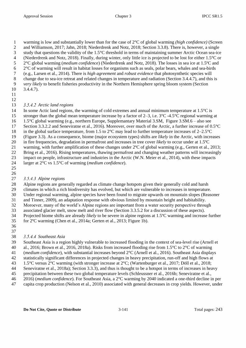
Approval Session Chapter 3 IPCC SR1.5
Do Not Cite, Quote or Distribute 3-141 Total pages: 243
warming is low and substantially lower than for the case of 2°C of global warming (high confidence) (Screen 1
and Williamson, 2017; Jahn, 2018; Niederdrenk and Notz, 2018; Section 3.3.8). There is, however, a single 2
study that questions the validity of the 1.5°C threshold in terms of maintaining summer Arctic Ocean sea-ice 3
(Niederdrenk and Notz, 2018). Finally, during winter, only little ice is projected to be lost for either 1.5°C or 4
2°C global warming (medium confidence) (Niederdrenk and Notz, 2018). The losses in sea ice at 1.5ºC and 5
2°C of warming will result in habitat losses for organisms such as seals, polar bears, whales and sea-birds 6
(e.g., Larsen et al., 2014). There is high agreement and robust evidence that photosynthetic species will 7
change due to sea-ice retreat and related changes in temperature and radiation (Section 3.4.4.7), and this is 8
very likely to benefit fisheries productivity in the Northern Hemisphere spring bloom system (Section 9
3.4.4.7). 10
11
12
Arctic land regions 13
In some Actic land regions, the warming of cold extremes and annual minimum temperature at 1.5°C is 14
stronger than the global mean temperature increase by a factor of 2–3, i.e. 3°C -4.5°C regional warming at 15
1.5°C global warming (e.g., northern Europe, Supplemantary Material 3.SM, Figure 3.SM.6 – also see 16
Section 3.3.2.2 and Seneviratne et al., 2016). Moreover, over much of the Arctic, a further increase of 0.5°C 17
in the global surface temperature, from 1.5 to 2°C may lead to further temperature increases of 2–2.5°C 18
(Figure 3.3). As a consequence, biome (major ecosystem types) shifts are likely in the Arctic, with increases 19
in fire frequencies, degradation in permafrost and increases in tree cover likely to occur under at 1.5ºC 20
warming, with further amplification of these changes under 2ºC of global warming (e.g., Gerten et al., 2013; 21
Bring et al., 2016). Rising temperatures, thawing permafrost and changing weather patterns will increasingly 22
impact on people, infrastructure and industries in the Arctic (W.N. Meier et al., 2014), with these impacts 23
larger at 2°C vs 1.5°C of warming (medium confidence). 24
25
26
Alpine regions 27
Alpine regions are generally regarded as climate change hotspots given their generally cold and harsh 28
climates in which a rich biodiversity has evolved, but which are vulnerable to increases in temperature. 29
Under regional warming, alpine species have been found to migrate upwards on mountain slopes (Reasoner 30
and Tinner, 2009), an adaptation response with obvious limited by mountain height and habitability. 31
Moroever, many of the world’s Alpine regions are important from a water security perspective through 32
associated glacier melt, snow melt and river flow (Section 3.3.5.2 for a discussion of these aspects). 33
Projected biome shifts are already likely to be severe in alpine regions at 1.5ºC warming and increase further 34
for 2ºC warming (Chen et al., 2014a; Gerten et al., 2013; Figure 1b). 35
36
37
Southeast Asia 38
Southeast Asia is a region highly vulnerable to increased flooding in the context of sea-level rise (Arnell et 39
al., 2016; Brown et al., 2016, 2018a). Risks from increased flooding rise from 1.5°C to 2°C of warming 40
(medium confidence), with substantial increases beyond 2°C (Arnell et al., 2016). Southeast Asia displays 41
statistically significant differences in projected changes in heavy precipitation, run-off and high flows at 42
1.5°C versus 2°C warming (with stronger increase at 2°C; (Wartenburger et al., 2017; Döll et al., 2018; 43
Seneviratne et al., 2018a); Section 3.3.3), and thus is thought to be a hotspot in terms of increases in heavy 44
precipitation between these two global temperature levels (Schleussner et al., 2016b; Seneviratne et al., 45
2016) (medium confidence). For Southeast Asia, a 2°C warming by 2040 indicated a one-third decline in per 46
capita crop production (Nelson et al., 2010) associated with general decreases in crop yields. However, under 47

Approval Session Chapter 3 IPCC SR1.5
Do Not Cite, Quote or Distribute 3-142 Total pages: 243
1.5°C of warming, significant risks for crop yield reduction in the region are avoided (Schleussner et al., 1
2016b). These changes pose significant risks for poor people in both rural regions and urban areas of 2
Southeast Asia (Section 3.4.10.1), with these risks being larger at 2°C of global warming compared to 1.5°C 3
of warming (medium confidence). 4
5
6
Southern Europe and the Mediterranean 7
The Mediterranean is regarded as a climate change hot spot both in terms of projected stronger warming of 8
the regional land-based hot extremes compared to the mean global temperature warming (e.g., Seneviratne et 9
al., 2016) and projected substantial decreases in mean precipitation with associated substantial increases in 10
dry spells. The latter is projected to increase from 7% to 11% when comparing regional impacts at 1.5°C 11
versus 2°C of global warming, respectively (Schleussner et al., 2016b). Low river flows are projected to 12
decrease in the Mediterranean under 1.5°C of global warming (Marx et al., 2018) with associated significant 13
decreases in high flows and floods (Thober et al., 2018), largely in response to reduced precipitation. The 14
median reduction in annual runoff almost double from about 9% (likely range: 4.5–15.5%) at 1.5°C to 17% 15
(likely range: 8–25%) at 2°C (Schleussner et al., 2016b). Similar results are found by (Döll et al., 2018). 16
Overall, there is high confidence of strong increases in dryness and decreases in water availability in the 17
Mediterranean and southern Europe from 1.5ºC to 2°C of global warming. Sea-level rise is expected to be 18
lower for 1.5ºC versus 2°C, lowering risks for coastal metropolitan agglomerations. The risks (with current 19
adaptation) related to water deficit in the Mediterranean are high for a global warming of 2°C, but can be 20
substantially reduced if global warming is limited to 1.5°C (Guiot and Cramer, 2016; Schleussner et al., 21
2016b; Donnelly et al., 2017; Section 3.3.4). 22
23
24
West Africa and the Sahel 25
West Africa and the Sahel are likely to experience increases in the number of hot nights and longer and more 26
frequent heat waves even if the global temperature increase is constrained to 1.5°C, with further increase at 27
2°C of global warming and beyond (e.g., Weber et al., 2018). Moreover, the daily rainfall intensity and run-28
off is expected to increase (low confidence) towards 2°C and higher global warming scenarios (Weber et al., 29
2018; Schleussner et al., 2016b), with these changes also being relatively large compared to the projected 30
changes at 1.5°C of warming. Moreover, increased risks are projected in terms of drought, particularly for 31
the pre-monsoon season (Sylla et al., 2015), with both rural and urban populations affected, and increasingly 32
so at 2°C of global warming as opposed to 1.5°C (Liu et al., 2018). Based on a World Bank (2013) study for 33
sub-Saharan Africa, a 1.5°C warming by 2030 might reduce the present maize cropping areas by 40%, 34
rendering these no longer suitable for current cultivars. Substantial negative impacts are also projected for 35
sorghum suitability in the western Sahel (Läderach et al., 2013; Sultan and Gaetani, 2016). Increase in 36
warming (2°C) by 2040 would result in further yield losses and damages to crops (i.e., maize, sorghum, 37
wheat, millet, groundnut, cassava). Schleussner et al. (2016b) consistently indicate reduced impacts on crop 38
yield for West Africa under 2°C vs 1.5°C of global warming. There is medium confidence that vulnerabilities 39
to water and food security in the African Sahel will be higher at 2°C compared to 1.5°C of global warming 40
(Cheung et al., 2016b; Betts et al., 2018), and at 2°C these vulnerabilities are expected to be worse (Sultan 41
and Gaetani, 2016; Lehner et al., 2017; Betts et al., 2018; Byers et al., 2018; Rosenzweig et al., 2018) (high 42
evidence). For global warming greater than 2°C, the western Sahel might experience the strongest drying and 43
experience serious food security issues (Ahmed et al., 2015; Parkes et al., 2018). 44
45
46

Approval Session Chapter 3 IPCC SR1.5
Do Not Cite, Quote or Distribute 3-143 Total pages: 243
Southern Africa 1
The southern African region is projected to be a climate change hot spot in terms of both hot extremes 2
(Figures 3.5 and 3.6) and drying (Figure 3.12). Indeed, temperatures have been rising in the subtropical 3
regions of southern Africa at approximately twice the global rate over the last five decades (Engelbrecht et 4
al., 2015). Associated elevated warming of the regional land-based hot extremes has occurred (Section 3.3; 5
Seneviratne et al., 2016). Increases in the numer of hot nights as well as longer and more frequent heat waves 6
are projected even if the global temperature increase is constrained to 1.5°C (high confidence), with further 7
increase at 2°C of global warming and beyond (high confidence) (Weber et al., 2018). 8
9
Moreover, the region is likely to become generally drier with reduced water availability under low mitigation 10
(Niang et al., 2014; Engelbrecht et al., 2015; Karl et al., 2015; James et al., 2017), with this particular risk 11
also prominent under 2°C of global warming and even 1.5ºC of warming (Gerten et al., 2013). Risks are 12
significantly reduced, however, under 1.5°C of global warming (Schleussner et al., 2016b). There are 13
consistent and statistically significant projected increases in risks of increased meteorological drought in 14
southern Africa at 2°C vs 1.5°C of warming (medium confidence). Despite the general rainfall reductions 15
projected for southern Africa, daily rainfall intensities are expected to increase over much of the region 16
(medium confidence), and increasingly so with further amounts of global warming. There is medium 17
confidence that livestock in southern Africa will experience increased water stress under both 1.5ºC and 2°C 18
of global warming, with negative economic consequences (e.g., Boone et al., 2017). The region is also 19
projected to experience reduced maize, sorghum and cocoa cropping area suitability as well as yield losses 20
under 1.5°C of warming, with further decreases towards 2°C of warming (World Bank, 2013). Generally, 21
there is high confidence that vulnerability to decreases in water and food availability is reduced at 1.5°C 22
versus 2°C for southern Africa (Betts et al., 2018), whilst at 2°C these are expected to be higher (Lehner et 23
al., 2017; Betts et al., 2018; Byers et al., 2018; Rosenzweig et al., 2018) (high confidence). 24
25
26
Tropics 27
Worldwide, the largest increases in the number of hot days are projected to occur in the tropics (Figure 3.7). 28
Moreover, the largest differences in the number of hot days for 1.5°C of global warming versus 2°C of 29
global warming are found in the tropics (Mahlstein et al., 2011). In tropical Africa, increases in the number 30
of hot nights, as well as longer and more frequent heat waves, are projected under 1.5°C of global warming, 31
with further increases under 2°C of global warming (Weber et al., 2018). Impact studies for major tropical 32
cereals reveal that yields of maize and wheat begin to decline with 1°C to 2°C of local warming in the 33
tropics. Schleussner et al. (2016b) project that constraining warming to 1.5ºC rather than 2ºC would avoid 34
significant risks of tropical crop yield declines in West Africa, South East Asia, and Central and South 35
America. There is limited evidence and thus low confidence that these changes may result in significant 36
population displacement from the tropics to the subtropics (e.g., Hsiang and Sobel, 2016). 37
38
39
Small islands 40
Small islands are well recognized to be very sensitive to climate change impact such as sea-level rise, 41
oceanic warming, precipitation, cyclones and coral bleaching (high agreement, robust evidence) (Nurse et 42
al., 2014; Ourbak and Magnan, 2017). Even at 1.5°C of global warming, the compounding impacts of 43
changes in rainfall, temperature, tropical cyclones and sea levels are likely to be significant across multiple 44
natural and human systems. There are potential benefits to Small Island Developing States (SIDS) from 45
avoided risks at 1.5ºC versus 2ºC, especially when coupled with adaptation efforts. In terms of sea-level rise, 46
by 2150, roughly 40,000 less people living in SIDS will be inundated in a 1.5°C world than in a 2°C world 47

Approval Session Chapter 3 IPCC SR1.5
Do Not Cite, Quote or Distribute 3-144 Total pages: 243
(Rasmussen et al., 2018). Constraining global warming to 1.5ºC would significantly reduce water stress 1
(about 25%) as compared to the projected water stress at 2ºC (e.g., Caribbean region, Karnauskas et al., 2
2018), and may enhance the ability of SIDS to adapt (Benjamin and Thomas, 2016). Up to 50% of the year is 3
projected to be very warm in the Caribbean for 1.5°C, with a further increase by up to 70 days for 2°C versus 4
1.5°C (Taylor et al., 2018). By limiting warming to 1.5°C instead of 2°C in 2050, risks of coastal flooding 5
(measured as the flood amplification factors for 100-year flood events) are reduced between 20 and 80% for 6
SIDS (Rasmussen et al., 2018). A case study of Jamaica with lessons for other Caribbean SIDS demonstrates 7
that the difference between 1.5ºC and 2C is likely to challenge livestock thermoregulation, resulting in 8
persistent heat stress for livestock (Lallo et al., 2018). 9
10
11
Fynbos and shrub biomes 12
The Fynbos and succulent Karoo biomes of South Africa are threatened systems that have been assessed in 13
AR5. Similar shrublands exists in the semi-arid regions of other continents, the Sonora-Mojave 14
Creosotebush-White Bursage Desert Scrub ecosystem in the USA being a prime example. Impacts accrue 15
across these systems with greater warming, with impacts at 2°C likely to be greater than those at 1.5°C 16
(medium confidence). Under 2°C of global warming, regional warming in drylands will be 3.2–4°C and 17
under 1.5°C of global warming, mean warming in drylands will still be about 3°C. The Fynbos biome in 18
southwestern South Africa is vulnerable to the increasing impact of fires under increasing temperatures and 19
drier winters (high confidence). The Fynbos biome is projected to lose about 20%, 45% and 80% of its 20
current suitable climate area under 1°C, 2°C and 3°C of warming with respect to present-day climate 21
(Engelbrecht and Engelbrecht, 2016), demonstrating the value of climate change mitigation in protecting this 22
rich centre of biodiversity. 23
24
25 Table 3.6: Emergence and intensity of climate change hot-spots under different degrees of global warming 26
Region and/or Phenomena
Warming of 1.5ºC or less
Warming of 1.5ºC-2°C Warming of 2°C - 3°C
Arctic sea-ice Arctic summer sea-ice is likely to be maintained. Habitat losses for organisms such as polar bears, whales, seals and sea-birds Benefits for arctic fisheries
The risk of an ice free Arctic in summer is ~ 50% or higher. Habitat losses for organisms such as polar bears, whales, seals and sea-birds may be critical if summers are ice-free Benefits for arctic fisheries
Arctic is very likely to be ice-free in summer. Critical habitat losses for organsims such as polar bears, whales, seals and sea-birds Benefits for arctic fisheries
Arctic land regions Cold extremes warm by a factor of 2.5-3, reaching up to 5.5 °C (high confidence) Biome shifts in the tundra and
Cold extremes warm by as much as 8 °C (high confidence) Larger intrusions of trees and shrubs in the tundra than under 1.5 °C of warming
Drastic regional warming is very likely A collapse in permafrost may

Approval Session Chapter 3 IPCC SR1.5
Do Not Cite, Quote or Distribute 3-145 Total pages: 243
Region and/or Phenomena
Warming of 1.5ºC or less
Warming of 1.5ºC-2°C Warming of 2°C - 3°C
permafrost deterioration is likely
is likely; larger but constrained losses in permafrost are likely
plausibly occur (low confidence); a drastic biome shift from tundra to boreal forest is possible (low confidence).
Alpine regions Severe shifts in biomes are likely Reduced grassland net primary productivity
Even more severe shifts are likely Increased risks for reduced grassland net primary productivity
Critical losses in alpine habitats are likely Increased risks for significantly reduced grassland net primary productivity
Southeast Asia Risks for increased flooding related to sea-level rise Increases in heavy precipitation events Significant risks of crop yield reductions are avoided
Higher risks for increased flooding related to sea-level rise (medium confidence) Stronger increases in heavy precipitation events (medium confidence) One third decline in per capita crop production (medium confidence)
Substantial increases in risks related to flooding from sea-level rise Substantial increased in heavy precipitation and high flow events Substantial reductions in crop yield
Small Islands Land of 40,000 less people inundated by 2150 on SIDS Risks for coastal flooding reduced by 20-80% for SIDS Fresh water stress reduced by 25% Increase in the
Tens of thousands displaced due to inundation of SIDS High risks for coastal flooding Fresh water stress from projected aridity Further increase of about 70 warm days per year
Substantial and wide-spread impacts through indundation of SIDS, coastal flooding, fresh water stress, persistent heat stress and loss of most coral reefs very likely
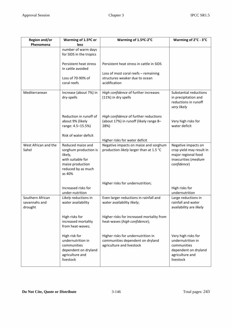
Approval Session Chapter 3 IPCC SR1.5
Do Not Cite, Quote or Distribute 3-146 Total pages: 243
Region and/or Phenomena
Warming of 1.5ºC or less
Warming of 1.5ºC-2°C Warming of 2°C - 3°C
number of warm days for SIDS in the tropics Persistent heat stress in cattle avoided Loss of 70-90% of coral reefs
Persistent heat stress in cattle in SIDS Loss of most coral reefs – remaining structures weaker due to ocean acidification
Mediterranean Increase (about 7%) in dry-spells Reduction in runoff of about 9% (likely range: 4.5–15.5%) Risk of water deficit
High confidence of further increases (11%) in dry spells High confidence of further reductions (about 17%) in runoff (likely range 8–28%) Higher risks for water deficit
Substantial reductions in precipitation and reductions in runoff very likely Very high risks for water deficit
West African and the Sahel
Reduced maize and sorghum production is likely, with suitable for maize production reduced by as much as 40% Increased risks for under-nutrition
Negative impacts on maize and sorghum production likely larger than at 1.5 °C Higher risks for undernutrition;
Negative impacts on crop yield may result in major regional food insecurities (medium confidence) High risks for undernutrition
Southern African savannahs and drought
Likely reductions in water availability High risks for increased mortality from heat-waves; High risk for undernutrition in communities dependent on dryland agriculture and livestock
Even larger reductions in rainfall and water availability likely; Higher risks for increased mortality from heat-waves (high confidence); Higher risks for undernutrition in communities dependent on dryland agriculture and livestock
Large reductions in rainfall and water availability are likely Very high risks for undernutrition in communities dependent on dryland agriculture and livestock

Approval Session Chapter 3 IPCC SR1.5
Do Not Cite, Quote or Distribute 3-147 Total pages: 243
Region and/or Phenomena
Warming of 1.5ºC or less
Warming of 1.5ºC-2°C Warming of 2°C - 3°C
Tropics Accumulated heat-wave duration up to two months (high confidence); 3% reduction in maize crop yield.
Accumulated heat-wave duration up to three months (high confidence); 7% reduction in maize crop yield.
Oppressive temperatures and accumulated heat-wave duration very likely to directly impact on human health, mortality and productivity Substantial reductions in crop yield very likely
Fynbos biome About 30% of suitable climate area lost (medium confidence)
Increased losses (about 45%) of suitable climate area (medium confidence)
Up to 80%of suitable climate area lost(medium confidence)
1
2
3.5.5 Avoiding regional tipping points by achieving more ambitious global temperature goals 3
4
Tipping points refer to critical thresholds in a system that, when exceeded, can lead to a significant change in 5
the state of the system, often with an understanding that the change is irreversible. An understanding of the 6
sensitivities of tipping points in the physical climate system, as well as ecosystems and human systems, is 7
essential for understanding the risks and opportunities from mitigation. This subsection reviews tipping 8
points across these three areas within the context of the different sensitivities to 1.5°C versus 2°C of global 9
warming. Sensitivities to less ambitious global temperature goals are also briefly reviewed. Moreover, how 10
integrated risks across physical, natural and human systems may accumulate to lead to the exceedance of 11
thresholds for particular systems is also analysed. The emphasis in this section is on the identification of 12
regional tipping points and their sensitivity to 1.5ºC and 2ºC of global warming – note that tipping points in 13
the global climate system, referred to as large scale singular events, have already been discussed in Section 14
3.5.2. A summary of regional tipping points is provided in Table 3.7. 15
16
17
Arctic sea-ice 18
Collins et al. (2013) discuss the loss of Artic sea ice in the context of potential tipping points. Climate 19
models have been used to assess whether a bifurcation exists that would lead to the irreversible loss of Arctic 20
sea ice (Armour et al., 2011; Boucher et al., 2012; Ridley et al., 2012) and to test whether summer sea ice 21
extent can recover after it has been lost (Schroeder and Connolley, 2007; Sedláček et al., 2011; Tietsche et 22
al., 2011). These studies do not find evidence of bifurcation and find that sea ice returns within a few years 23
of its loss, leading Collins et al. (2013) to conclude that there is little evidence for a tipping point in the 24
transition from perennial to seasonal ice cover. Studies do not find evidence of irreversibility or tipping 25
points, and suggest that year-round sea ice could return with years given a suitable climate (medium 26
confidence) (Schroeder and Connolley, 2007; Sedláček et al., 2011; Tietsche et al., 2011). 27
28
Approval Session Chapter 3 IPCC SR1.5
Do Not Cite, Quote or Distribute 3-148 Total pages: 243
Tundra 1
Tree-growth in tundra-dominated landscapes is strongly constrained by the number of days above 0°C. A 2
potential tipping points exists, where the number of days below 0°C decrease to the extent that tree fraction 3
increases significantly. Tundra-dominated landscapes have warmed more than the global average over the 4
last century (Settele et al., 2014), with associated increases in fires and permafrost degradation (Bring et al., 5
2016; DeBeer et al., 2016; Jiang et al., 2016; Yang et al., 2016). Both of these processes facilitate conditions 6
for woody species establishment in tundra areas, and the eventual transition of the tundra to boreal forest. 7
The number of investigations into how the tree-fraction may respond in the Arctic to different degrees of 8
global warming is limited, and generally indicative that substantial increases will likely occur gradually (e.g., 9
Lenton et al., 2008). Abrupt changes only plausible at levels of warming significantly larger than 2°C (low 10
confidence) and are to occur in conjunction with a collapse in permafrost (Drijfhout et al., 2015). 11
12
13
Permafrost 14
Widespread thawing of permafrost potentially makes a large carbon store (estimated to be twice the size of 15
the atmospheric store, Dolman et al., 2010) vulnerable to decomposition, which would lead to further 16
increases in atmospheric carbon dioxide and methane and hence further global warming. This feedback loop 17
between warming and the release of greenhouse gas from thawing tundra represents a potential tipping point. 18
However, the carbon released from thawing permafrost is projected to be restricted to 0.12-0.25 Gt C a-1 to 19
the atmosphere in a 2ºC world, and to 0.08-0.16 Gt C a-1for 1.5ºC (Burke et al., 2006), and thus do not 20
represent a tipping point (medium confidence). At higher degrees of global warming, in the order of 3°C, a 21
different type of tipping point in permafrost may be reached. A single model projection (Drijfhout et al., 22
2015) suggests that higher temperatures may induce a smaller ice fraction in soils in the tundra, leading to 23
more rapidly warming soils and a positive feedback mechanism that results in permafrost collapse (low 24
confidence). The disparity between the multi-millennial timescales of soil carbon accumulation and 25
potentially rapid decomposition in a warming climate implies that the loss of this carbon to the atmosphere is 26
essentially irreversible (Collins et al., 2013). 27
28
29
Asian monsoon 30
It is the pressure gradient between the Indian Ocean and Asian continent that at a fundamental level 31
determines the strength of the Asian monsoon. As land masses warm faster than the oceans, a general 32
strengthening of this gradient, and hence monsoons, may be expected under global warming (e.g., Lenton et 33
al., 2008). Additional factors such as changes in albedo induced by aerosols and snow-cover change may 34
also affect temperature gradients and consequently pressure gradients and the strength of the monsoon. In 35
fact, it has been estimated that an increase of the landmass albedo to 0.5 would represent a tipping point 36
resulting in the collapse of the monsoon system (Lenton et al., 2008). The overall impacts of the various 37
types of radiative forcing under different emission scenarions are more subtle, with a weakening of the 38
monsoon north of about 25°N in East Asia and a strengthening south of this latitude projected by (Jiang and 39
Tian, 2013) under high and modest emission scenarios. Increases in the intensity of monsoon precipitation is 40
likely under low mitigation (AR5). Given that scenarios at 1.5°C or 2°C would include a substantially 41
smaller radiative forcing than those assessed in the studies of Jiang and Tian (2013) there is low confidence 42
regarding changes in monsoons at these low global warming levels, as well as regarding the differences 43
between responses at 1.5°C versus 2°C levels of global warming. 44
45
46

Approval Session Chapter 3 IPCC SR1.5
Do Not Cite, Quote or Distribute 3-149 Total pages: 243
West African monsoon and the Sahel 1
Earlier work has identified 3°C of global warming as a tipping point leading to a significant strengthening of 2
the West African monsoon and subsequent wettening (and greening) of the Sahel and Saharah (Lenton et al., 3
2008). AR5 (Niang et al., 2014) as well as more recent research through the Coordinated Regional 4
Downscaling Experiment for Africa (CORDEX-AFRICA) provide a more uncertain view, however, in terms 5
of the rainfall futures of the Sahel under low mitigation futures. Even if a wetter Sahel should materialize 6
under 3°C of global warming (low confidence), it should be noted that there will be significant offsets in the 7
form of strong regional warming and related adverse impacts on crop yield, livestock mortality and human 8
health under such low mitigation futures (Engelbrecht et al., 2015; Sylla et al., 2016; Weber et al., 2018b) 9
10
11
Rain forests 12
A large portion of rainfall over the world’s largest rainforests are recirculated (e.g., Lenton et al., 2008), 13
which raises the concern that deforestation may trigger a threshold in reduced forest cover leading to 14
pronounced forest dieback. For the Amazon, this deforestation threshold has been estimated to be 40% 15
(Nobre et al., 2016). Global warming of 3°C–4°C may also, independent of deforestation, represent a tipping 16
point that results in a significant dieback of the Amazon forest, with a key forcing mechanism being stronger 17
El Niño envents bringing more frequent droughts to the region (Nobre et al., 2016). Increased fire 18
frequencies under global warming may interact with and accelerate deforestation, particularly during periods 19
of El Niño induced droughts (Lenton et al., 2008; Nobre et al., 2016). Global warming of 3°C is projected to 20
reduce the extent of tropical rainforest in Central America, with biomass productivity being reduced by more 21
than 50%, and a large replacement of rainforest by savanna and grassland (Lyra et al., 2017). Overall, 22
modelling studies (Huntingford et al., 2013; Nobre et al., 2016) and observational constraints (Cox et al., 23
2013) suggest that pronounced rainforest dieback may only be triggered at 3°C–4 °C (medium confidence), 24
although pronounced biomass losses may occur at 1.5°C and 2°C of global warming. 25
26
27
Boreal forests 28
Boreal forests are likely to experience higher local warming than the global average (WGII AR5: Collins et 29
al., 2013). Increased disturbance from fire, pests and heat related mortality may affect in particular the 30
southern boundary of boreal forests (Gauthier et al., 2015) (medium confidence), with these impacts accruing 31
with greater warming and thus impacts at 2°C would be expected to be greater than those at 1.5°C (medium 32
confidence). A tipping point for significant dieback of the boreal forests is thought to exist, where increased 33
tree mortality will result in the creation of large regions of open woodlands and grasslands, which would 34
favour further regional warming and increased fire frequencies, thus inducing a powerful positive feedback 35
mechanism (Lenton et al., 2008; Lenton, 2012). This tipping point has been estimated to exist between 3 and 36
4°C of global warming (Lucht et al., 2006; Kriegler et al., 2009) (low confidence), but given the complexities 37
of the various forcing mechanisms and feedback processes this is thought to be an uncertain estimate. 38
39
40
Heat-waves, unprecedented heat and human health 41
Increases in ambient temperature are linearly related with hospitalizations and deaths (so there isn’t a tipping 42
point per se) once specific thresholds are exceeded. It is plausible that coping strategies will not be in place 43
for many regions, with potentially significant impacts on communities with low adaptive capacity, 44
effectively representing the occurrence of a local/regional tipping point. In fact, even if global warming is 45
restricted to below 2°C, taking into consideration urban heat island effects, there could be a substantial 46
increase in the occurrence of deadly heatwaves in cities, with the impacts similar at 1.5°C and 2°C, but 47

Approval Session Chapter 3 IPCC SR1.5
Do Not Cite, Quote or Distribute 3-150 Total pages: 243
substantially larger than under the present climate (Matthews et al., 2017). At +1.5°C, twice as many 1
megacities as present (such as Lagos, Nigeria, and Shanghai, China) are likely to become heat stressed, 2
potentially exposing more than 350 million more people to deadly heat stress by 2050. At +2°C warming, 3
Karachi (Pakistan) and Kolkata (India) could expect annual conditions equivalent to their deadly 2015 4
heatwaves (medium confidence). These statistics imply a tipping point in the extent and scale of heat-wave 5
impacts. However, these projections do not integrate adaptation to projected warming, for instance, cooling 6
that could be achieved with more reflective roofs and urban surfaces overall (Akbari et al., 2009; Oleson et 7
al., 2010). 8
9
10
Agricultural systems: key staple crops 11
A large number of studies consistently indicate that maize crop yield will be negatively affected under 12
increased global warming, with negative impacts being higher under 2°C of warming than at 1.5°C of warming 13
(e.g., Niang et al., 2014; Schleussner et al., 2016b; J. Huang et al., 2017; Iizumi et al., 2017). Under 2°C of 14
global warming, losses of 8-14% are projected in global maize production (Bassu et al., 2014). Under more 15
than 2°C of global warming, regional losses are projected to be about 20% if they co-occur with reductions in 16
rainfall (Lana et al., 2017). These changes may be classified as incremental rather than representing a tipping 17
point. Large-scale reductions in maize crop yield including the potential for the collapse of this crop in some 18
regions may exist under 3°C or more of global warming (low confidence) (e.g., Thornton et al., 2011). 19
20
21
Agricultural systems: livestock in the tropics and subtropics 22
The potential impacts of climate change on livestock (Section 3.4.6) and in particular direct impacts through 23
inceased heat-stress has been less well studied than impacts on crop yield, in particular from the perspective 24
of critical thresholds being exceeded. A case study of Jamaica reveals that the difference in heat stress for 25
livestock between 1.5C and 2C is likely to exceed the limits for normal thermoregulation and result in 26
persistent heat stress for livestock animals (Lallo et al., 2018). It is plausible that this finding holds for 27
livestock production in both tropical and subtropical regions more generally (medium confidence) (see 28
Section 3.4.6). It is plausible that under 3°C of global warming, significant reductions in the areas suitable 29
for livestock production occur (low confidence) due to strong increases in regional temperatures in the 30
tropics and subtropics (high confidence). Thus, regional tipping points in the viability of livestock production 31
may well exist, but little evidence quantifying such changes exist. 32
33 Table 3.7: Summary of enhanced risks in the exceedance of regional tipping points under different global 34
temperature goals. 35 36
Tipping point Warming of 1.5ºC or less Warming of 1.5ºC-2°C Warming of up to 3°C
Arctic sea-ice Arctic summer sea-ice is likely to be maintained. Sea-ice changes reversible under suitable climate restoration
The risk of an ice free Arctic in summer is ~ 50% or higher. Sea-ice changes reversible under suitable climate restoration
Arctic is very likely to be ice-free in summer. Sea-ice changes reversible under suitable climate restoration
Tundra Decrease in number of growing degree days
Further decreases in number of growing
Potential for an abrupt increase in tree-

Approval Session Chapter 3 IPCC SR1.5
Do Not Cite, Quote or Distribute 3-151 Total pages: 243
Tipping point Warming of 1.5ºC or less Warming of 1.5ºC-2°C Warming of up to 3°C
below 0°C Abrupt increases in tree-cover are unlikely
degree days below 0°C Abrupt increased in tree cover are unlikely
fraction (low confidence)
Permafrost 21-37% reduction in permafrost
2 million km2 more permafrost maintained than under 2°C of global warming (medium confidence) 0.08-0.16 Gt C a-1 released Irreversible loss of stored carbon
35-47% reduction in permafrost 0.12-0.25 Gt C a-1 released Irreversible loss of stored carbon
Potential for permafrost collapse (low confidence)
Asian Monsoon Low confidence in projected changes
Low confidence in projected changes
Increases in the intensity of monsoon precipitation likely.
West African monsoon and the Sahel
Uncertain changes, unlikely that a tipping point is reached
Uncertain changes, unlikely that tipping point is reached
Strengthening of monsoon and wettening and greening of Sahel and Saharah (low confidence) Negative associated impacts through increase in extreme temperature events
Rainforests Reduced biomass, deforestation and fire increases pose uncertain risks to forest dieback
Larger biomass reductions than under 1.5 °C warming, deforestation and fire increases pose uncertain risk to forest dieback
Potential tipping point leading to pronounced forest dieback (medium confidence)
Boreal forests Increased tree mortality at southern boundary of boreal forest (medium confidence)
Further increases in tree mortality at southern boundary of boreal forest (medium confidence)
Potential tipping point for significant dieback of boreal forest (low confidence)
Heat-waves, unprecedented heat
Substantial increase in occurrence of potentially
Substantial increase in potentially deadly
Substantial increase in potentially deadly

Approval Session Chapter 3 IPCC SR1.5
Do Not Cite, Quote or Distribute 3-152 Total pages: 243
Tipping point Warming of 1.5ºC or less Warming of 1.5ºC-2°C Warming of up to 3°C
and human health deadly heat-waves likely More than 350 million more people exposed to deadly heat by 2050 under a midrange population growth scenario
heat-waves likely Annual occurrence of heat-waves similar to deadly 2015 heat-waves in India and Pakistan
heat-waves very likely
Key staple crops Global maize crop reductions of about 10%
Larger reductions in maize crop production that under 1.5°C of about 15%
Drastic reductions in maize crop globally and in Africa (high confidence), of 20% or more; potential tipping point for collapse of maize crop in some regions (low confidence)
Livestock in the tropics and subtropics
Increased heat-stress Onset of persistent heat-stress (medium confidence)
Persistent heat-stress likely.
1
2

Approval Session Chapter 3 IPCC SR1.5
Do Not Cite, Quote or Distribute 3-153 Total pages: 243
[START BOX 3.6 HERE] 1
Economic Damages from Climate Change 2
3
Balancing of the costs and benefits of mitigation is challenging because estimating the value of climate 4
change damages depends on multiple parameters whose appropriate values have been debated for decades 5
(for example, the appropriate value of the discount rate) or that are very difficult to quantify (for example, 6
the value of non-market impacts; the economic effects of losses in ecosystem services; and the potential for 7
adaptation, which is dependent on the rate and timing of climate change and on the socioeconomic content) 8
(see Cross-Chapter Box 5 in Chapter 2 for the definition of the social cost of carbon, and discussion of the 9
economics of 1.5°C-consistent pathways and the social cost of carbon, including the impacts of inequality on 10
the social cost of carbon). 11
12
Global economic damages of climate change are smaller under warming of 1.5°C than 2°C in 2100 (Warren 13
et al., 2018c). The mean net present value of the costs of damages from warming in 2100 for 1.5°C and. 2°C 14
(including costs associated with climate change-induced market and non-market impacts, impacts due to sea 15
level rise, and impacts associated with large scale discontinuities) are $54 and $69 trillion, respectively, 16
relative to 1961-1990. 17
18
Values of the social cost of carbon vary when tipping points are included. The social cost of carbon in the 19
default setting of the Dynamic Integrated Climate-Economy (DICE) model increases from $15/tCO2 to $116 20
(range 50-166)/tCO2 when large-scale singularities or ‘tipping elements’are incorporated (Y. Cai et al., 2016; 21
Lemoine and Traeger, 2016). Lemoine and Traeger (2016) included optimization calculations that minimize 22
welfare impacts resulting from the combination of climate change risks and climate change mitigation costs, 23
showing that welfare is minimized if warming is limited to 1.5ºC. These calculations excluded the large 24
health co-benefits that accrue when greenhouse gas emissions are reduced (Shindell 2018; Section 3.4.7.1) 25
26
The economic damages of climate change in the USA are projected to be large (Hsiang et al., 2017; Yohe, 27
2017). Although not specifically related to 1.5°C warming, Hsiang et al. (2017) concluded that the USA 28
could lose 2.3% Gross Domestic Product (GDP) per degree of global warming. Yohe (2017) calculated 29
transient temperature trajectories from a linear relationship with contemporaneous cumulative emissions 30
under a median no-policy baseline trajectory that brings global emissions to roughly 93 GtCO2 per year by 31
the end of the century (Fawcett et al., 2015), with 1.75°C per 1000 GtCO2 as the median estimate (Yohe, 32
2017). Associated aggregate economic damages in decadal increments through the year 2100 are estimated 33
in terms of the percentage loss of GDP at the median, 5th percentile, and 95th percentile transient temperature 34
(Hsiang et al., 2017). The results for the baseline no-policy case indicate that economic damages along 35
median temperature change and median damages (median-median) reach 4.5% of GDP by 2100, with an 36
uncertainty range of 2.5% and 8.5% resulting from different combinations of temperature change and 37
damages. Avoided damages from achieving a 1.5oC temperature limit along the median-median case is 38
nearly 4% (range 2.0 – 7.0%) by 2100. Avoided damages from achieving a 2oC temperature limit is lower: 39
3.5% (range 1.8% - 6.5%). Avoided damages from achieving 1.5oC vs. 2oC is modest; it is about 0.35% 40
(range 0.20 – 0.65%) by 2100. The values of achieving either temperature limit do not diverge significantly 41
until 2040, when their difference tracks between 0.05% and 0.13%; the differences between the two 42
temperature targets begin to diverge substantially in the second half of the century. 43
[END BOX 3.6 HERE] 44
45

Approval Session Chapter 3 IPCC SR1.5
Do Not Cite, Quote or Distribute 3-154 Total pages: 243
Implications of different 1.5ºC and 2ºC pathways 1
2
This section provides an overview on specific aspects of the mitigation pathways considered compatible with 3
1.5°C global warming. Some of these aspects are also addressed in more detail in the Cross-Chapter Boxes 7 4
and 8 in this Chapter. 5
6
7
3.6.1 Gradual vs overshoot in 1.5ºC scenarios 8
9
All 1.5°C scenarios from Chapter 2 include some overshoot above 1.5°C global warming during the 21st 10
century (Chapter 2, Cross-Chapter Box 8 in this Chapter). The level of overshoot may also depend on natural 11
climate variability. An overview of possible outcomes of a 1.5°C-consistent mitigation scenarios for changes 12
in physical climate at the time of overshoot and by 2100 is provided in the Cross-Chapter Box 8 on “1.5°C 13
warmer worlds”. Cross-Chapter Box 8 also highlights the implications of overshoots. 14
15
16
3.6.2 Non-CO2 implications and projected risks of mitigation pathways 17
18
Land use changes 19
Risks arising from Land use changes in Mitigation Pathways 20
21
In mitigation pathways, land use change is affected by many different mitigation options. First of all, 22
mitigation of non-CO2 emissions from agricultural production can shift agricultural production between 23
regions via trade of agricultural commodities. Secondly, protection of carbon rich ecosystems such as 24
tropical forests constrains area for agricultural expansion. Thirdly, also demand side mitigation measures 25
such as les consumption of resource intensive commodities (animal products) or food waste reductions 26
reduce pressure on land (Popp et al., 2017; Rogelj et al., 2018). Finally, Carbon Dioxide Removal (CDR) is a 27
key component of most, but not all mitigation pathways presented in the literature to date which constrain 28
warming to 1.5°C or 2°C. Typically, CDR measures that require land can include Bioenergy with Carbon 29
Capture and Storage (BECCS), afforestation and reforestation (AR), soil carbon sequestration, direct air 30
capture, biochar, and enhanced weathering (see Cross-Chapter Box 7 in this Chapter). These potential 31
methods are assessed in Section 4.3.7. 32
33
In cost-effective Integrated Assessment Modelling (IAM) pathways recently developed to be consistent with 34
limiting warming to 1.5°C, use of CDR in the form of BECCS and AR are also fundamental elements 35
(Chapter 2; Popp et al., 2017; Hirsch et al., 2018; Rogelj et al., 2018; Seneviratne et al., 2018c). The land-36
use footprint of CDR deployment in 1.5°C-consistent pathways can be substantial (Section 2.3.4, Figure 37
2.11), even though IAMs predominantly rely on second generation biomass and assume future productivity 38
increases in agriculture. 39
40
A body of literature has explored potential consequences of large scale use of CDR. In this case, the 41
corresponding land footprint by the end of the century could be extremely large, with estimates including: up 42
to 18% of the land surface being used (Wiltshire and Davies-Barnard, 2015); vast acceleration of the loss of 43
primary forest and natural grassland (Williamson, 2016) leading to increased greenhouse gas emissions (P. 44
Smith et al., 2013, Smith et al., 2015); potential loss of up to 10% of the current forested lands to biofuels 45
(Yamagata et al., 2018). Other estimates reach 380-700 Mha/21-64% of current arable cropland (Section 46

Approval Session Chapter 3 IPCC SR1.5
Do Not Cite, Quote or Distribute 3-155 Total pages: 243
4.3.7); while Boysen et al. (2017) find that in a scenario in which emission reductions were sufficient only to 1
limit warming to 2.5ºC, use of CDR to limit warming further to 1.7ºC would result in conversion of 1.1-1.5 2
Gha of land – implying enormous losses of both cropland and natural ecosystems (Boysen et al., 2017). 3
Newbold et al. (2015) find that biodiversity loss in the scenario Representative Concentation Pathway 4
(RCP)2.6 could be greater than that in RCP4.5 and RCP6.0, in which there is more climate change but less 5
land use change. Risks to biodiversity conservation and agricultural production are therefore projected to 6
result from large-scale bioenergy deployment pathways (P. Smith et al., 2013; Tavoni and Socolow, 2013). 7
One study explores an extreme mitigation strategy encouraging biofuel expansion sufficient to limit warming 8
to 1.5ºC, which finds that this is more disruptive to land use and crop prices than the climate change impacts 9
of +2.0 ºC world which has a larger climate signal and lower mitigation requirement (Ruane et al., 2018). 10
However, it should again be emphasized that many of the pathways explored in Chapter 2 of this report 11
follow strategies that explore how to reduce these issues. Chapter 4 provides an assessment of the land 12
footprint of various CDR technologies (Section 4.3.7). 13
14
The degree to which BECCS would have these large land-use footprints depends on the source of the 15
bioenergy used, and the scale at which BECCS is deployed. Whether there is competition with food 16
production and biodiversity depends on the governance of land use, agricultural intensification, trade, 17
demand for food (in particular meat), feed and timber, and the context of the whole supply chain (Section 18
4.3.7, Fajardy and Mac Dowell, 2017; Booth, 2018; Sterman et al., 2018). 19
20
The more recent literature reviewed in Chapter 2 explores pathways which limit warming to 2°C or below 21
and achieve a balance between sources and sinks of CO2, using BECCS that relies on second-generation (or 22
even third generation) biofuels, or which relies on changes in diet or more generally, management of food 23
demand, or CDR options such as forest restoration (see Chapter 2, Bajželj et al., 2014). Overall this 24
literature explores how to reduce the issues of competition for land with food production and with natural 25
ecosystems (in particular forests) (see Cross-Chapter Box 1 in Chapter 1, van Vuuren et al., 2009; Haberl et 26
al., 2010, 2013; Bajželj et al., 2014; Daioglou et al., 2016; Fajardy and Mac Dowell, 2017). 27
28
Some IAMs manage this transition by effectively protecting carbon stored on land and focussing on the 29
conversion of pasture area into both forest area and bioenergy cropland. Some IAMs explored 1.5°C 30
consistent pathways with demand side measures (such as dietary changes) and efficiency gains such as 31
agricultural changes (Sections 2.3.4, 2.4.4) which lead to a greatly reduced CDR deployment and 32
consequently land use impacts (van Vuuren et al., 2018). However, in reality whether this CDR (and more 33
broadly, bioenergy in general) has large adverse impacts on environmental and societal goals depends in 34
large parts on the governance of land use (Obersteiner et al., 2016; Bertram et al., 201; Humpenöder et al. 35
2018; Section 2.3.4). 36
37
Rates of sequestration of 3.3 GtC/ha require 970 Mha of afforestation and reforestation (Smith et al., 2015). 38
Humpenöder et al. (2014) estimates that in least cost pathways afforestation would cover 2800 Mha by the 39
end of the century to constrain warming to 2°C. Hence, the amount of land considered if least-cost 40
mitigation is implemented by afforestation and reforestation could be up to 3 to 5 times greater than that 41
required by BECCS, depending on the forest management used. However, not all of the land footprint of 42
CDR need be in competition with biodiversity protection. Where reforestation is the restoration of natural 43
ecosystems, this benefits both carbon sequestration and conservation of biodiversity and ecosystem services 44
(Section 4.3.7) and can contribute to the achievement of the Aichi targets under the Convention on 45
Biological Diversity (CBD) (Leadley et al., 2016). However, reforestation is often not defined in this way 46
(Stanturf et al., 2014, Section 4.3.8) and the ability to deliver biodiversity benefits is strongly dependent on 47

Approval Session Chapter 3 IPCC SR1.5
Do Not Cite, Quote or Distribute 3-156 Total pages: 243
the precise nature of the reforestation, which has many different interpretations in different contexts and can 1
often include agroforestry rather than restoration of pristine ecosystems (Pistorious and Kiff, 2017). 2
However, ‘natural climate solutions’ defined as conservation, restoration, and improved land management 3
actions that increase carbon storage and/or avoid greenhouse gas emissions across global forests, wetlands, 4
grasslands, and agricultural lands is estimated to have the potential to provide 37% of cost-effective CO2 5
mitigation needed through 2030 consistent with a >66% chance of holding warming to below 2°C (Griscom 6
et al., 2017). 7
8
Any reductions in agricultural production driven by climate change and/or land management decisions 9
related to CDR may (e.g., Nelson et al., 2014a; Dalin & Rodríguez-Iturbe, 2016) or may not (Muratori et al., 10
2016) affect food prices. However, these studies do not consider the deployment of second-generation 11
bioenergy crops (instead of first-generation) for which the land footprint can be much smaller. 12
Irrespective of any mitigation-related issues, in order for ecosystems to adapt to climate change, land use 13
would also need to be carefully managed to allow biodiversity to disperse to areas that become newly 14
climatically suitable for it Section 3.4.1) as well as protecting the areas where the climate still remains 15
suitable in the future. This implies a need for a considerable expansion of the protected area network 16
(Warren et al., 2018a), either to protect existing natural habitat or to restore it (perhaps through reforestation, 17
see above). At the same time, adaptation to climate change in the agricultural sector (Rippke et al., 2016) 18
can require transformational as well as new approaches to land use management; whilst in order to meet the 19
rising future food demand of a growing human population, additional land is projected to be needed to be 20
brought into production, unless there are large increases in agricultural productivity (Tilman et al., 2011) yet 21
future rates of deforestation may be underestimated in the existing literature (Mahowald et al., 2017a). 22
Hence, reforestation may be associated with significant co-benefits if implemented so as to restore natural 23
ecosystems (high confidence). 24
25
26
Biophysical feedbacks on regional climate associated with land use changes 27
Changes in the biophysical characteristics of the land surface are known to have an impact on local and 28
regional climates through changes in albedo, roughness, evapotranspiration and phenology that can lead to a 29
change in temperature and precipitation. This includes changes in land use through agricultural 30
expansion/intensification (e.g., Mueller et al., 2016) or reforestation/revegetation endeavours (e.g., Feng et 31
al., 2016; Sonntag et al., 2016; Bright et al., 2017) and changes in land management (e.g., Luyssaert et al., 32
2014; Hirsch et al., 2017) that can involve double cropping (e.g., Jeong et al., 2014; Mueller et al., 2015; 33
Seifert and Lobell, 2015), irrigation (e.g., Lobell et al, 2009; Sacks et al., 2009; Cook et al., 2011; Qian et al., 34
2013; de Vrese et al., 2016; Pryor et al., 2016; Thiery et al., 2017), no-till farming and conservation 35
agriculture (e.g., Lobell et al., 2006; Davin et al., 2014) and wood harvest (e.g., Lawrence et al., 2012). 36
Hence, the biophysical impacts of land use changes are an important topic to assess in the context of low-37
emissions scenarios (e.g., (van Vuuren et al., 2011b), in particular for 1.5°C warming levels (see also Cross-38
Chapter Box 7 in this Chapter). 39
40
The magnitude of the biophysical impacts is potentially large for temperature extremes. Indeed, both changes 41
induced by modifications in moisture availability and irrigation, or by changes in surface albedo, tend to be 42
larger (i.e., stronger cooling) for hot extremes than for mean temperatures (e.g., (Seneviratne et al., 2013; 43
Davin et al., 2014; Wilhelm et al., 2015; Hirsch et al., 2017; Thiery et al., 2017). The reasons for reduced 44
moisture availability are related to a strong contribution of moisture deficits to the occurrence of hot 45
extremes in mid-latitude regions (Mueller and Seneviratne, 2012; Seneviratne et al., 2013). In the case of 46
surface albedo, cooling associated with higher albedo (e.g., in the case of no-till farming) is more effective at 47
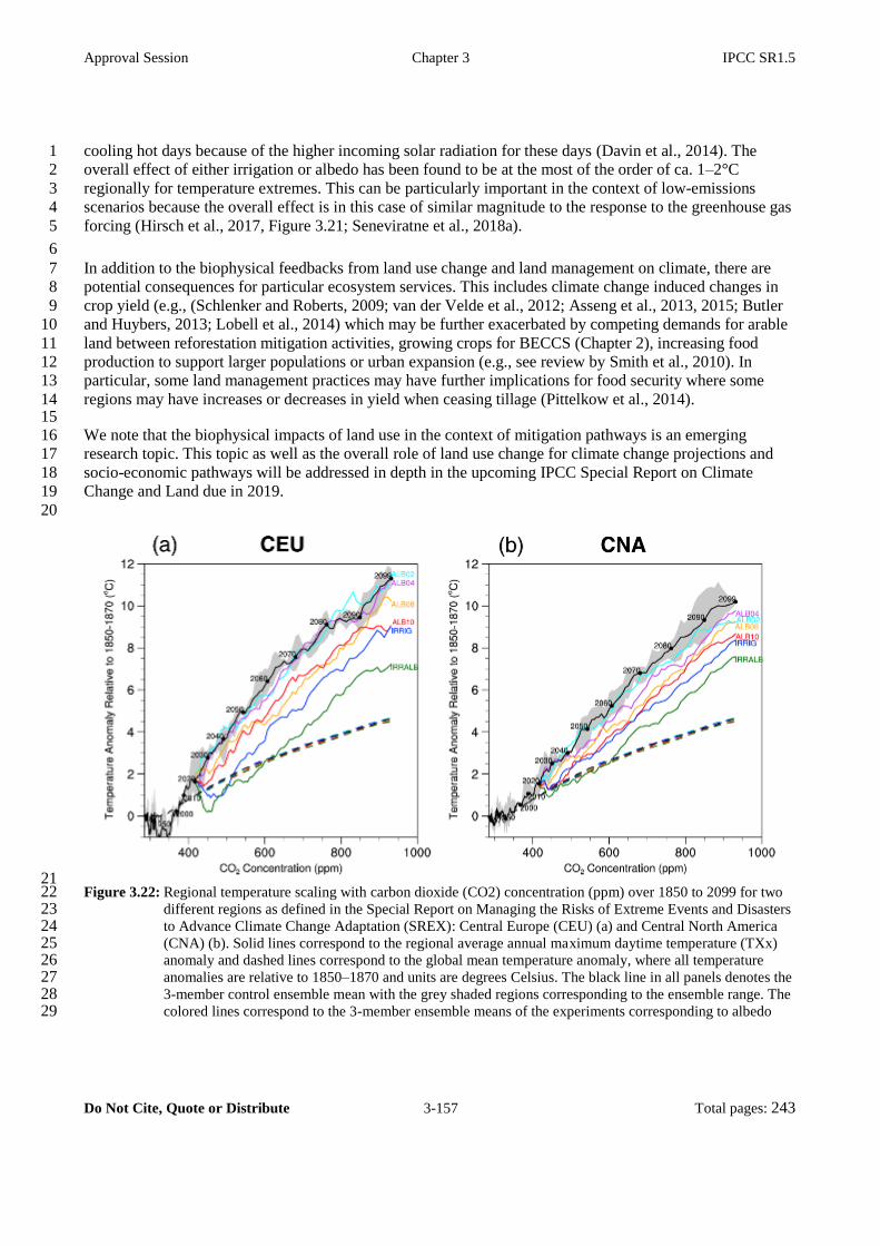
Approval Session Chapter 3 IPCC SR1.5
Do Not Cite, Quote or Distribute 3-157 Total pages: 243
cooling hot days because of the higher incoming solar radiation for these days (Davin et al., 2014). The 1
overall effect of either irrigation or albedo has been found to be at the most of the order of ca. 1–2°C 2
regionally for temperature extremes. This can be particularly important in the context of low-emissions 3
scenarios because the overall effect is in this case of similar magnitude to the response to the greenhouse gas 4
forcing (Hirsch et al., 2017, Figure 3.21; Seneviratne et al., 2018a). 5
6
In addition to the biophysical feedbacks from land use change and land management on climate, there are 7
potential consequences for particular ecosystem services. This includes climate change induced changes in 8
crop yield (e.g., (Schlenker and Roberts, 2009; van der Velde et al., 2012; Asseng et al., 2013, 2015; Butler 9
and Huybers, 2013; Lobell et al., 2014) which may be further exacerbated by competing demands for arable 10
land between reforestation mitigation activities, growing crops for BECCS (Chapter 2), increasing food 11
production to support larger populations or urban expansion (e.g., see review by Smith et al., 2010). In 12
particular, some land management practices may have further implications for food security where some 13
regions may have increases or decreases in yield when ceasing tillage (Pittelkow et al., 2014). 14 15
We note that the biophysical impacts of land use in the context of mitigation pathways is an emerging 16
research topic. This topic as well as the overall role of land use change for climate change projections and 17
socio-economic pathways will be addressed in depth in the upcoming IPCC Special Report on Climate 18
Change and Land due in 2019. 19
20
21 Figure 3.22: Regional temperature scaling with carbon dioxide (CO2) concentration (ppm) over 1850 to 2099 for two 22
different regions as defined in the Special Report on Managing the Risks of Extreme Events and Disasters 23 to Advance Climate Change Adaptation (SREX): Central Europe (CEU) (a) and Central North America 24 (CNA) (b). Solid lines correspond to the regional average annual maximum daytime temperature (TXx) 25 anomaly and dashed lines correspond to the global mean temperature anomaly, where all temperature 26 anomalies are relative to 1850–1870 and units are degrees Celsius. The black line in all panels denotes the 27 3-member control ensemble mean with the grey shaded regions corresponding to the ensemble range. The 28 colored lines correspond to the 3-member ensemble means of the experiments corresponding to albedo 29

Approval Session Chapter 3 IPCC SR1.5
Do Not Cite, Quote or Distribute 3-158 Total pages: 243
+0.02 (cyan), albedo +0.04 (purple), albedo + 0.08 (orange), albedo +0.10 (red), irrigation on (blue), and 1 irrigation with albedo +0.10 (green). Adapted from Hirsch et al. (2017). 2
3
4
Atmospheric compounds (aerosols and methane) 5
There are multiple pathways that could be used to limit anthropogenic climate change, and the details of the 6
pathways will change the climate impacts on humans and ecosystems. Anthropogenic driven changes in 7
aerosols cause important modifications to global climate (Bindoff et al., 2013a; Boucher et al., 2013b; P. Wu 8
et al., 2013; Sarojini et al., 2016; H. Wang et al., 2016). Enforcement of strict air quality policies may lead to 9
a large decrease in cooling aerosols emissions in the next few decades. These aerosol emission reductions 10
may cause a comparable warming to the increase in greenhouse gases by mid-21st century in the low CO2 11
pathways (Kloster et al., 2009; Navarro et al., 2017), especially in the low CO2 pathways (Cross Chapter Box 12
1; Sections 2.2.2 and 2.3.1). Because aerosol effects on the energy budget are regional, strong regional 13
changes in precipitation changes from aerosols may occur if aerosols emissions are reduced for air quality or 14
as a co-benefit from switches to sustainable energy sources (H. Wang et al., 2016). Thus regional impacts, 15
especially on precipitation, are very sensitive to 1.5ºC-consistent pathways (Z. Wang et al., 2017). 16
17
Pathways which rely strong on reductions in methane (CH4) versus CO2 will reduce warming in the short-18
term because methane is such a stronger and shorter-lived greenhouse gas, but will be warmer in the long 19
term because of the much longer residence time of CO2 (Myhre et al., 2013; Pierrehumbert, 2014). In 20
addition, the dominant loss mechanism for methane is atmospheric photooxidation. This conversion modifies 21
ozone formation and destruction in the troposphere and stratosphere, and therefore modifies the contribution 22
of ozone to radiative forcing, as well as feedbacks onto the oxidation rate of methane itself (Myhre et al., 23
2013). Focusing on pathways and policies which both improve air quality and reduce climate impacts can 24
serve to provide multiple co-benefits (Shindell et al., 2017), and these pathways are discussed in detail in 25
Sections 4.3.7 and 5.4.1; and Cross Chapter Box 12 in Chapter 5. 26
27
Atmospheric aerosols and gases can also modify the land and ocean uptake of anthropogenic carbon dioxide, 28
but some compounds enhance uptake, while others reduce uptake (Ciais et al., 2013) (Section 2.6.2). While 29
CO2 emissions tend to encourage greater uptake of carbon by the land and the ocean (Ciais et al., 2013), 30
methane emissions can enhance ozone pollution, depending on nitrogen oxides, volatile organic compounds, 31
and other organic species concentrations, and ozone tends to reduce land productivity (Myhre et al., 2013; B. 32
Wang et al., 2017). Aside from inhibiting land vegetation productivity, ozone may also alter the CO2, CH4 33
and nitrogen (N2O) exchange at the land-atmosphere interface and transform the global soil system from a 34
sink to a source of carbon (B. Wang et al., 2017). Aerosols and associated nitrogen-based compounds tend to 35
enhance the uptake of carbon dioxide in land and ocean systems through the deposition of nutrients and 36
modification of climate (Ciais et al., 2013; Mahowald et al., 2017b). 37
38
[START BOX Cross-Chapter Box 7] 39
Cross-Chapter Box 7: Land-Based Carbon Dioxide Removal, in Relation to 1.5°C Warming 40
41
Lead Authors: Marcos Buckeridge (Brazil), Sabine Fuss (Germany), Markku Kanninen (Finland), Joeri 42
Rogelj (Austria/Belguim), Sonia I. Seneviratne (Switzerland), Raphael Slade (United Kingdom), Rachel 43
Warren (United Kingdom). 44
45
Climate and land form a complex system characterised by multiple feedback processes and the potential for 46
non-linear responses to perturbation. Climate determines land cover and the distribution of vegetation 47

Approval Session Chapter 3 IPCC SR1.5
Do Not Cite, Quote or Distribute 3-159 Total pages: 243
affecting above and below ground carbon stocks. At the same time, land cover influences global climate 1
through altered biogeochemical processes (e.g. atmospheric composition and nutrient flow into oceans), and 2
regional climate through changing biogeophysical processes (including albedo, hydrology, transpiration and 3
vegetation structure) (Forseth, 2010). 4
5
Greenhouse Gas (GHG) fluxes related to land use are reported in the Agriculture, Forestry and Other Land 6
Use sector (AFOLU) and comprise about 25% (about 10–12 GtCO2eqyr-1) of anthropogenic GHG emissions 7
(P. Smith et al., 2014). Reducing emissions from land use, and land use change are thus an important 8
component of low-emissions mitigation pathways (Clarke et al., 2014), particularly as land-use emissions 9
can be influenced by human actions such as deforestation, afforestation, fertilisation, irrigation, harvest, and 10
other aspects of cropland, grazing land and livestock management (Paustian et al., 2006; Griscom et al., 11
2017; Houghton and Nassikas, 2018). 12
13
In the IPCC Fifth Assessment Report, the vast majority of scenarios assessed with a 66% or better chance of 14
limiting global warming to 2°C by 2100 included Carbon Dioxide Removal (CDR) – typically about 10 15
GtCO2 per year in 2100 or about 200–400 GtCO2 over the course of the century (Smith et al., 2015; van 16
Vuuren et al., 2016). These Integrated Assessment Model (IAM) results were predominately achieved by 17
using bioenergy with carbon capture and storage (BECCS) and/or afforestation and reforestation (AR). 18
Virtually all scenarios that either limit peak or end-of-century warming to 1.5°C also use land intensive CDR 19
technologies (Rogelj et al., 2015; Holz et al., 2017; Kriegler et al., 2017; Fuss et al., 2018; van Vuuren et al., 20
2018). Again, afforestation and reforestation (AR) (Sections 2.3, 4.3.7); and BECCS (Sections 4.3.2., 4.3.7) 21
predominate. Other CDR options such as the application of biochar to soil, soil carbon sequestration, and 22
enhanced weathering (Section 4.3.7) are not yet widely incorporated in IAMs, but their deployment would 23
also necessitate the use of land and/or changes in land management. 24
25
IAMs provide a simplified representation of land use and, with only a few exceptions, they do not include 26
biophysical feedback processes (e.g. albedo and evapotranspiration effects) (Kreidenweis et al., 2016) 27
despite the importance of these processes for regional climate, in particular hot extremes (Seneviratne et al., 28
2018c; section 3.6.2.2). The extent, location, and impacts of large-scale land-use change described by 29
existing IAMs can also be widely divergent depending on model structure, scenario parameters, modelling 30
objectives, and assumptions (including land availability and productivity) (Prestele et al., 2016; Alexander et 31
al., 2017; Popp et al., 2017; Seneviratne et al., 2018d). Despite these limitations, IAM scenarios effectively 32
highlight the extent and nature of potential land-use transitions implicit in limiting warming to 1.5oC . 33
34
Cross-Chapter Box 7 Table 1, presents a comparison of the five CDR options assessed in this report. This 35
illustrates that if deployed at a scale -e.g. 12 GtCO2yr-1 in 2100-, BECCS and AR would have a substantial 36
land and water footprint. Wether this footprint results in adverse impacts, for example on biodiversity or 37
food production, depends on the existence and effectiveness of measures to conserve land carbon stocks, 38
limit the expansion of agriculture at the expense of natural ecosystems, and increase agriculture productivity 39
(Bonsch et al., 2016; Obersteiner et al., 2016; Bertram et al., 2018; Humpenöder et al., 2018). In comparison, 40
the land and water footprints of enhanced weathering, soil carbon sequestration and biochar application are 41
expected to be far less per GtCO2 sequestered. These options may offer potential co-benefits by providing an 42
additional source of nutrients or reducing N2O emissions, but they are also associated with potential side-43
effects. Enhanced weathering would require massive mining activity, and providing feedstock for biochar 44
would require additional land, even though a proportion of the required biomass is expected to come from 45
residues (Woolf et al., 2010; Smith, 2016). For the terrestrial CDR options permanence and saturation are 46
important considerations, making their viability and long-term contributions to carbon reduction targets 47

Approval Session Chapter 3 IPCC SR1.5
Do Not Cite, Quote or Distribute 3-160 Total pages: 243
uncertain. 1
2
The technical, political, and social feasibility of scaling up and implementing land-intensive CDR 3
technologies (Cross-Chapter Box 3 in Chapter 1) is recognised to present considerable potential barriers to 4
future deployment (Boucher et al., 2013a; Fuss et al., 2014, 2018; Anderson and Peters, 2016; Williamson, 5
2016; Vaughan and Gough, 2016; Minx et al., 2017, 2018; Nemet et al., 2018; Strefler et al., 2018; Vaughan 6
et al., 2018). To investigate the implications of restricting CDR options should these barriers prove difficult 7
to overcome IAM studies (Section 2.3.4) have developed scenarios that limit (either implicity or explicity) 8
the use of BECCS and bioenergy (Krey et al., 2014; Bauer et al., 2018; Rogelj et al., 2018), or BECCS and 9
afforestation (Strefler et al., 2018). Alternative strategies to limit future reliance on CDR have also been 10
examined including increased electrification, agricultural intensification, behavioral change and dramatic 11
improvements in energy and material efficiency (Bauer et al., 2018; Grübler, 2018; van Vuuren et al., 2018). 12
Somewhat counterintuitively, scenarios that seek to limit the deployment of BECCs may result in increased 13
land use through greater deployment of bioenergy, and afforestation (Krey et al., 2014; Krause et al., 2017; 14
Bauer et al., 2018; Rogelj et al., 2018) (Chapter 2, Box 2.1). Scenarios aiming to minimize the total human 15
land footprint (including land for food, energy, and climate mitigation) also result in land use change, for 16
example by postulating that increases in agricultural efficiency and changes in diet can enable land use, for 17
example by postulating that increases in agricultural efficiency and changes in diet can enable land use 18
switching from food crop production to energy crop production without altering the overall agricultural area 19
(Grübler, 2018). 20
21
The impacts of changing land use are highly context, location and scale dependent (Robledo‐ Abad et al., 22
2017). The supply of biomass for CDR (e.g. energy crops) has received particular attention. The literature 23
identifies regional examples of where the use of land to produce biofuels might be sustainably increased 24
(Jaiswal et al., 2017), where biomass markets could contribute to the provision of ecosystem services (Dale 25
et al., 2017), and where bioenergy could increase the resilience of production systems and contribute to rural 26
development (Kline et al., 2017). Yet studies of global biomass potential provide only limited insight into the 27
local feasibility of supplying large quantities of biomass on a global scale (Slade et al., 2014). Concerns 28
about large scale use of biomass for CDR include a range of potential consequences including: greatly 29
increased demand for freshwater use, increased competition for land, loss of biodiversity and/or impacts on 30
food security (Heck et al., 2018; Section 3.6.2.1). The short versus long term carbon impacts of substituting 31
biomass for fossil fuels (in large part determined by feedstock choice) also remain a source of contention 32
(Schulze et al., 2012; Jonker et al., 2014; Booth, 2018; Sterman et al., 2018). 33
34
AR can also present trade-offs between biodiversity, carbon sequestration and water use, and has a higher 35
land footprint per ton of CO2 removed (Cunningham et al., 2015; Naudts et al., 2016; Smith et al., 2018). For 36
example, changing forest management to strategies towards faster growing species, greater residue 37
extraction, and shorter rotations may have a negative impact on biodiversity (de Jong et al., 2014). In 38
contrast, reforestation of degraded land with native trees can have substantial benefits for biodiversity 39
(Section 3.6). Despite these constraints the potential for increased carbon sequestration through improved 40
land stewardship measures is considered to be substantial (Griscom et al., 2017). 41
42
Evaluating the synergies and trade-offs between mitigation and adaptation actions, resulting land and climate 43
impacts, and the myriad issues related to land-use governance will be essential to better understand the future 44
role of CDR technologies. This will be further addressed in the IPCC Special Report on Climate Change and 45
Land (SRCCL) due to be published in 2019. 46
47

Approval Session Chapter 3 IPCC SR1.5
Do Not Cite, Quote or Distribute 3-161 Total pages: 243
Key messages: 1
2
Cost-effective strategies to limit peak or end-of-century warming to 1.5°C all include enhanced GHG 3
removals in the AFOLU sector as part of their portfolio of measures (high agreement, robust evidence). 4
5
Large-scale deployment of land-based CDR would have far reaching implications for land and water 6
availability (high agreement, robust evidence). This may impact food production, biodiversity and the 7
provision of other ecosystem services (high agreement, medium evidence) 8
9
The impacts of deploying land-based CDR at scale can be reduced if a wider portfolio of CDR options is 10
deployed, and if increased mitigation effort focusses on strongly limiting demand for land, energy and 11
material resources including lifestyle and dietary change (high agreement, medium evidence). 12
13
Afforestation and reforestation may be associated with significant co-benefits if implemented appropriately, 14
but feature large land water footprints if deployed at scale (medium agreement, medium evidence). 15
16 17 Cross-Chapter Box 7, Table 1: Comparison of land-based carbon removal options 18 Sources: a assessed ranges by Fuss et al. (2018); see Figures in Section 4.3.7 for full literature range; b based on 2100 19 estimate for mean potentials by (Smith et al., 2015). Note that biophysical impacts of land-based CDR options besides 20 albedo changes (e.g., through changes in evapotranspiration related to irrigation or land cover/use type) are not displayed. 21 22
Option Potential
s a
Cost a Requi
red
land b
Req
uire
d
wate
r b
Impac
t on
nutrie
nts b
Impact on
albedo b
Saturation & permanence a
GtCO2
y−1
$ per
tCO2
Mha
GtCO
2−1
km3
GtC
O2−1
Mt N,
P,
K y−1
No units No units
BECCS 0.5-5 100-
200
31-58 60 Variabl
e
Variable,
depends on
source of
biofuel
(higher
albedo for
crops than for
forests) and
on land
management
(e.g., no-till
farming for
crops)
Long-term governance of
storage;
limits on rates of bioenergy
production and carbon
sequestration
Afforestation
&
Reforestation
0.5-3.6 5-50 80 92 0.5 Negative; or
reduced
GHG benefit
where not
negative
Saturation of forests; vulnerable
to disturbance; post-AR forest
management essential

Approval Session Chapter 3 IPCC SR1.5
Do Not Cite, Quote or Distribute 3-162 Total pages: 243
Enhanced
Weathering
2-4 50-200 3 0.4 0 0 Saturation of soil; residence time
from months to geological time
scale
Biochar 0.3-2 30-120 16-
100
0 N:8.2,
P:2.7,
K:19.1
0.08–0.12 Mean residence times between
decades to centuries depending
on soil type, management, and
environmental conditions
Soil Carbon
Sequestratio
n
2.3-5 0-100 0 0 N:21.8,
P:5.5,
K:4.1
01 Soil sinks saturate and can
reverse if poor management
practices were to resume
[END BOX Cross-Chapter Box 7] 1 2
3
3.6.3 Implictions beyond the end of the century 4
5
Sea ice 6
Sea ice is often cited as a tipping point in the climate system (Lenton, 2012). Detailed modelling of sea ice 7
(Schroeder and Connolley, 2007; Sedláček et al., 2011; Tietsche et al., 2011), however, suggests that 8
summer sea ice can return within a few years after its artificial removal for climates in the late 20th and early 9
21st centuries. Further studies (Armour et al., 2011; Boucher et al., 2012; Ridley et al., 2012) remove sea ice 10
by raising CO2 concentrations and study subsequent regrowth by lowering CO2. These studies also suggest 11
changes in Arctic sea ice are neither irreversible nor exhibit bifurcation behavior. It is therefore plausible that 12
the extent of Arctic sea ice may quickly re-equilibrate to end-of-century climate in the event of an overshoot 13
scenario. 14
15
16
Sea level 17
The impacts of policy decisions related to anthropogenic climate change will have a profound impact on sea 18
level not only for the remainder of this century but for many millennia to come (Clark et al., 2016). On these 19
long timescales, 50 m of sea level rise are potentially possible (Clark et al., 2016). While it is virtually 20
certain that sea level will continue to rise well beyond 2100, the amount of rise depends on future 21
cumulative emissions (Church et al., 2013) as well as their profile over time (Bouttes et al., 2013; Mengel et 22
al., 2018). Marzeion et al. (2018) find that 28–44% of present-day glacier volume is unsustainable in the 23
present-day climate, so that it would eventually (over the course of a few centuries) melt, even if there were 24
no further climate change. Some components of sea level rise, such as thermal expansion, are only reversible 25
on centennial timescales (Bouttes et al., 2013; Zickfeld et al., 2013), while the contribution from ice sheets 26
may not be reversible under any plausible future scenario (see below). 27
28
Based on the sensitivities summarized by Levermann et al. (2013), the contributions of thermal expansion 29
(0.20–0.63 m C-1) and glaciers (0.21 m C-1 falling at higher degrees of warming mostly because of the 30
depletion of glacier mass, with a possible total of ~0.6 m) amount to 0.5–1.2 m and 0.6–1.7 m in 1.5 and 2C 31
warmer worlds, respectively. The bulk of Sea Level Rise (SLR) on greater than centennial timescales will 32
therefore be contributed by the two continental ice sheets of Greenland and Antarctica, whose existence is 33
threatened on multi-millennial timescales. 34
35
For Greenland, where melting from the ice sheet’s surface is important, a well-documented instability exists 36

Approval Session Chapter 3 IPCC SR1.5
Do Not Cite, Quote or Distribute 3-163 Total pages: 243
where the surface of a thinning ice sheet encounters progressively warmer air temperatures that further 1
promote melt and thinning. A useful indicator associated with this instability is the threshold at which annual 2
mass loss from the ice sheet by surface melt exceeds mass gain by snowfall. Previous estimates (Gregory and 3
Huybrechts, 2006) put this threshold about 1.9ºC to 5.1C above preindustrial period. More recent analyses, 4
however, suggest that this threshold sits between 0.8ºC and 3.2C with a best estimate at 1.6C (Robinson et 5
al., 2012). The continued decline of the ice sheet after this threshold has been passed is highly dependent on 6
future climate and varies between about 80% loss after 10,000 years to complete loss after as little as 2000 7
years (contributing ~6 m to SLR). 8
9
The Antarctic ice sheet, in contrast, loses the mass gained by snowfall as outflow and subsequent melt to the 10
ocean (either directly from the underside of floating ice shelves or indirectly by the melt of calved icebergs). 11
The long-term existence of this ice sheet is also affected by a potential instability (the Marine Ice Sheet 12
Instability, MISI), which links outflow (or mass loss) from the ice sheet to water depth at the grounding line 13
(the point at which grounded ice starts to float and becomes an ice shelf) so that retreat into deeper water (the 14
bedrock underlying much of Antarctica slopes downwards towards the centre of the ice sheet) leads to 15
further increases in outflow and promotes yet further retreat (Schoof, 2007). More recently, a variant on this 16
mechanism has been postulated in which an ice cliff forms at the grounding line which retreats rapidly 17
though fracture and iceberg calving (DeConto and Pollard, 2016). There is a growing body of evidence 18
(Golledge et al., 2015; DeConto and Pollard, 2016) that large-scale retreat may be avoided in emission 19
scenarios such as Representative Concentration Pathway (RCP)2.6 but that higher-emission RCP scenarios 20
could lead to the loss of the West Antarctic ice sheet and sectors in East Antarctica, although the duration 21
(centuries or millennia) and amount of mass loss during such as collapse is highly dependent on model 22
details and no consensus yet exists. Current thinking (Schoof, 2007) suggests that retreat may be irreversible, 23
although a rigorous test has yet to be made. In this context, overshoot scenarios, especially of higher 24
magnitude or longer duration, could be anticipated to increase the risk of such irreversible retreat. 25
26
The assessment also noted that the collapse of marine sectors of the Antarctic ice sheet could lead to Global 27
Mean Sea Level (GMSL) rise above the likely range, and that there was medium confidence that this 28
additional contribution ‘would not exceed several tenths of a metre during the 21st century’ (Church et al., 29
2013). 30
31
The multi-centennial evolution of the Antarctic ice sheet is considered in papers by DeConto and Pollard 32
(2016) and Golledge et al. (2015). Both suggest that RCP2.6 is the only RCP scenario leading to long-term 33
contributions to GMSL of below 1.0 m. The long-term committed future of Antarctica (and GMSL 34
contribution at 2100) are complex and require further detailed process-based modelling, however a 35
threshold in this contribution may be present close to 1.5ºC. 36
37
38
Permafrost 39
The slow rate of permafrost thaw introduces a lag between the transient degradation of near-surface 40
permafrost and contemporary climate, so that the equilibrium response is expected to be 25–38% greater 41
than the transient response simulated in climate models (Slater and Lawrence, 2013). The long-term, 42
equilibrium Arctic permafrost loss to global warming is analyzed by Chadburn et al. (2017). They use an 43
empirical relation between recent mean annual air temperatures and the area underlain by permafrost coupled 44
to CMIP5 stabilization projections to 2300 for RCP2.6 and RCP4.5. Their estimate of the sensitivity of 45
permafrost to warming is 2.9–5.0 million km2 C-1 (1 standard deviation confidence interval), which suggests 46
that stabilizing climate at 1.5C as opposed to 2C would reduce the area of eventually permafrost loss by 47

Approval Session Chapter 3 IPCC SR1.5
Do Not Cite, Quote or Distribute 3-164 Total pages: 243
roughly 2 million km2 (stabilizing at 56–83% as opposed to 43–72% of 1960–1990 levels). This work 1
combined with the assessment of Collins et al. (2013) on the link of global warming and permafrost loss, 2
leads to the assessment that permafrost extent would be appreciably greater in a 1.5°C world compared to a 3
2°C world (medium confidence, limited evidence). 4
5
6
Knowledge gaps 7
8
Most scientific literature specific to global warming of 1.5°C is only just emerging. This has led to 9
differences in the amount of information available and gaps across the various sections of this chapter. In 10
general, the number of impact studies specifically focused on 1.5°C lags behind climate change projections in 11
general, due in part to the dependence of the former on the latter. There are also insufficient studies focusing 12
on regional changes, impacts and consequences at +1.5°C and +2°C of global warming. 13
14
The following gaps have been identified with respect to tools, methodologies and understanding in the 15
current scientific literature specific to Chapter 3. The gaps identified here are not comprehensive but 16
highlight general areas for improved understanding, especially of global warming at 1.5°C as compared to 17
2°C and higher. 18
19
20
3.7.1 Gaps in Methods and Tools 21
22
Regional and global climate model simulations for low-emission scenarios such as a 1.5°C world. 23
24
Robust probabilistic models which separate the relatively small signal between 1.5°C versus 2°C from 25
background noise, and which handle the many uncertainties associated with non-linearities, 26
innovations, overshoot, local scales, latent or lagging responses in climate. 27
28
Projections of risks under a range of climate and development pathways required to understand how 29
development choices affect the magnitude and pattern of risks, and to provide better estimates of the 30
range of uncertainties. 31
32
More complex and integrated socio-ecological models for predicting the response of terrestrial 33
ecosystems to climate and models which are increasingly capable of separating climate effects from 34
those associated with human activities. 35
36
Tools for informing local and regional decision-making especially when the signal is ambiguous at 1.5°C 37
and/or reverses sign at higher levels of global warming. 38
39
40
3.7.2 Gaps in Understanding 41
42
Earth systems and 1.5oC: 43 44
The cumulative effects of multiple stresses and risks (e.g., increased storm intensity interacting with sea 45
level rise and the effect on coastal people; feedback on wetlands due to climate change and human 46

Approval Session Chapter 3 IPCC SR1.5
Do Not Cite, Quote or Distribute 3-165 Total pages: 243
activities). 1
2
Feedbacks associated with changes in land use/cover for low-emissions scenarios, for example, 3
feedback from changes in forest cover, food production, and biofuel production, Bio-Energy with 4
Carbon Capture and Storage (BECCS), and associated unquantified biophysical impacts. 5
6
The distinct impacts of different overshoot scenarios depending on (a) the peak temperature of the 7
overshoot, (b) the length of the overshoot period, and (c) the associated rate of change in global 8
temperature over the time period of the overshoot. 9
10
Physical and chemical characteristics of a 1.5oC world: 11 12
Critical thresholds for extreme events (e.g., drought, inundation) between 1.5°C and 2°C, for different 13
climate models and projections. All aspects of storm intensity and frequency as a function of climate 14
change, especially for 1.5°C and 2°C worlds, and the impact of changing storminess on storm surge, 15
damage and coastal flooding at regional and local scales. 16
17
The timing and implications of the release of stored carbon in Arctic permafrost in a 1.5°C world and for 18
climate stabilization by the end of the century. 19
20
Antarctic ice sheet dynamics, global sea level, and links between seasonal and year-long sea ice in both 21
polar regions. 22
23
Terrestrial and freshwater systems 24 25
The dynamics between climate change, freshwater resources, and socioeconomic impacts for lower 26
levels of warming. 27
28
How the health of vegetation is likely to change, carbon storage in plant communities and landscapes, 29
and phenomena such as the fertilization effect. 30
31
The risks associated with species’ maladaptation in response to climatic changes (e.g., effect of late 32
frosts), and questions associated with issues such as the consequences of species advancing their spring 33
phenology in response to warming, and the interaction between climate change, range shifts and local 34
adaptation in a 1.5°C world. 35
36
The biophysical impacts of land use in the context of mitigation pathways. 37
38
Ocean Systems 39 40
Deep sea processes and risks to deep sea habitats and ecosystems. 41
42
Changes in ocean chemistry in a 1.5°C world, including how decreasing ocean oxygen content, ocean 43
acidification, and changes to activity of multiple ion species, will affect natural and human systems. 44
45
How ocean circulation is changing towards a 1.5°C and 2°C world, for example, vertical mixing, deep 46

Approval Session Chapter 3 IPCC SR1.5
Do Not Cite, Quote or Distribute 3-166 Total pages: 243
ocean processes, currents, and their impacts on weather patterns at regional to local scales. 1
2
The impacts of changing ocean conditions at 1.5°C and 2°C warming on food webs, disease, invading 3
species, coastal protection, fisheries and human well-being, especially as organisms modify their 4
biogeographical ranges within a changing ocean. 5
6
Specific linkages between food security and changing coastal and ocean resources. 7
8
Human systems 9 10
The impacts of global and regional climate change at 1.5°C on food distribution, nutrition, poverty, 11
tourism, coastal infrastructure, and public health, particularly for developing nations. 12
13
Health and well-being risks in the context of socio-economic and climate change at 1.5°C, especially in 14
key areas such as occupational health, air quality and infectious disease. 15
16
Micro-climates at urban/city scales and their associated risks for natural and human systems, within 17
cities and interactions with surrounding areas. For example, current projections do not integrate 18
adaptation to projected warming by taking into account cooling that could be achieved through a 19
combination of revised building codes, zoning, and land use to build more reflective roofs and urban 20
surfaces that reduce urban heat islands. 21
22
Implications of climate change at 1.5°C on livelihoods and poverty, on rural communities, indigenous 23
groups and marginalised people. 24
25
The changing levels of risk in terms of extreme events (including storms and heat events), especially 26
with respect to people being displaced or having to migrate away from sensitive and exposed systems 27
such as small islands, low lying coasts and deltas. 28
29
30
31
32

Approval Session Chapter 3 IPCC SR1.5
Do Not Cite, Quote or Distribute 3-167 Total pages: 243
Cross-Chapter Box 8: 1.5ºC Warmer Worlds 1
2
Lead Authors: Myles R. Allen (United Kingdom), Marcos Buckeridge (Brazil), Kristie L. Ebi (United 3
States of America), Neville Ellis (Australia), Ove Hoegh-Guldberg (Australia), Richard J. Millar (United 4
Kingdom), Antony J. Payne (United Kingdom), Joeri Rogelj (Austria/Belguim), Roland Séférian (France), 5
Sonia I. Seneviratne (Switzerland), Petra Tschakert (Australia), Rachel Warren (United Kingdom). 6
7
Contributing Authors: Richard Wartenburger (Germany/Switzerland). 8
9
Introduction 10 11
The Paris Agreement includes goals of stabilizing Global Mean Surface Temperature (GMST) well below 12
2°C and 1.5°C above preindustrial period, in the longer term. There are several aspects, however, that remain 13
open regarding what a ‘1.5°C warmer world’ could be like, in terms of mitigation (Chapter 2) and adaptation 14
(Chapter 4), as well as in terms of projected warming and associated regional climate change (Chapter 3), 15
overlaid on anticipated and differential vulnerabilities (Chapter 5). Alternative ‘1.5°C warmer worlds’ 16
resulting from mitigation and adaptation choices, as well as from climate variability (climate ‘noise’), 17 can be vastly different as highlighted in this Cross-Chapter Box. In addition, the range of models 18
underlying 1.5°C projections can be substantial and needs factoring in. 19
20
Key questions3: 21 22
What is a 1.5°C global mean warming, how is it measured, and what temperature increase does it 23 imply for single locations and at specific times? GMST corresponds to the globally averaged 24
temperature of the Earth derived from point-scale ground observations or computed in climate models 25
(Chapters 1 and 3). GMST is additionally defined over a given time frame, for example, averaged over a 26
month, a year, or multiple decades. Because of climate variability, a climate-based global mean 27
temperature typically needs to be defined over several decades (typically 20 or 30 years; Chapter 3, 28
Section 3.2). Hence, whether or when global temperature reaches 1.5°C depends to some extent on the 29
choice of preindustrial reference period, whether 1.5°C refers to total or human-induced warming, and 30
which variables and coverage are used to define GMST change (Chapter 1). By definition, because 31
GMST is an average in time and space, there will be locations and time periods in which 1.5°C warming 32
is exceeded, even if the global mean temperature warming is at 1.5°C. In some locations, these 33
differences can be particularly large (Cross-Chapter Box 8, Figure 1). 34
35
What is the impact of different climate models for projected changes in climate at 1.5°C global 36 warming? The range between single model simulations of projected regional changes at 1.5°C GMST 37
warming can be substantial for regional responses (Chapter 3, Section 3.3). For instance, for the warming 38
of cold temperature extremes in a 1.5°C warmer world, some model simulations project a 3°C warming 39
and others more than 6°C warming in the Arctic land areas (Cross-Chapter Box 8, Figure 2). For warm 40
temperature extremes in the contiguous United States, the range of model simulations includes colder 41
temperatures than pre-industrial (-0.3°C) and a warming of 3.5°C (Cross-Chapter Box 8, Figure 2). Some 42
regions display an even larger range (e.g., 1–6°C regional warming in hot extremes in Central Europe at 43
1.5°C warming, Chapter 3, Sections 3.3.1 and 3.3.2). This large spread is due both to modelling 44
3FOOTNOTE: Part of this discussion is based on Seneviratne et al. (2018e)

Approval Session Chapter 3 IPCC SR1.5
Do Not Cite, Quote or Distribute 3-168 Total pages: 243
uncertainty and internal climate variability. While the range is large, it also highlights risks that can be 1
avoided with near certainty in a 1.5°C warmer world compared to worlds at higher levels of warming 2
(e.g., an 8°C warming in cold extremes in the Arctic is not reached at 1.5°C global warming in the multi-3
model ensemble, but could happen at 2°C global warming, Cross-Chapter Box 8, Figure 2). Inferred 4
projected ranges of regional responses (mean value, minimum and maximum) for different mitigation 5
scenarios from Chapter 2 are displayed in Cross-Chapter Box 8, Table 1. 6
7
8 9
Cross-Chapter Box 8, Figure 1: Range of projected realized temperature at 1.5°C (due to stochastic noise and 10 model-based spread). Temperature with a 25% chance of occurrence at any location within 10-year time frames 11 corresponding to GMST anomalies of 1.5°C (Coupled Model Intercomparison Project Phase 5 (CMIP5) multi-model 12 ensemble). The plots display at each location the 25th percentile (Q25, left) and 75th percentile (Q75, right) values of 13 mean temperature (Tmean), yearly maximum day-time temperature (TXx), yearly minimum night-time temperature 14 (TNn), sampled from all time frames with GMST anomalies of 1.5°C in Representative Concentration Pathway 15 (RCP)8.5 model simulations of the CMIP5 ensemble. From (Seneviratne et al., 2018b). 16 17

Approval Session Chapter 3 IPCC SR1.5
Do Not Cite, Quote or Distribute 3-169 Total pages: 243
1 2
Cross-Chapter Box 8, Figure 2: Spread of projected multi-model changes in minimum annual night-time temperature 3 (TNn) in the Arctic land (left) and in maximum annual day-time temperature (TXx) in the contiguous United States as a 4 function of mean global warming in climate simulations. The multi-model range (due to model spread and internal climate 5 variability) is indicated in red shading (minimum and maximum value based on climate model simulations). The multi-6 model mean value is displayed with solid red and blue lines for two emissions pathways (blue : Representative 7 Concentration Pathway (RCP)4.5; red : RCP8.5). The dashed red line indicates projections for a 1.5°C warmer world. 8 The dashed black line displays the 1:1 line. [after Seneviratne et al., 2016]. 9
10
What is the impact of emissions pathways with, versus without, an overshoot? All mitigation 11
pathways projecting less than 1.5°C global warming over or at the end of the 21st century, include some 12
probability of overshooting 1.5°C. These pathways include some time periods with higher warming than 13
1.5°C in the course of the coming decades and/or some probability of not reaching 1.5°C (Chapter 2; 14
Section 2.2). This is inherent to the difficulty of limiting global warming to 1.5°C given that we are 15
already very close to this warming level. The implications of overshooting are large for risks to natural 16
and human systems, especially if the temperature at peak warming is high, because some risks may be 17
long-lasting and irreversible, such as the loss of many ecosystems (Chapter 3, Box 3.4). The chronology 18
of emission pathways and their implied warming is also important for the more slowly evolving parts of 19
the Earth system, such as those associated with sea level rise. In addition, for several types of risks, the 20
rate of change may be of most relevance (Loarie et al., 2009; LoPresti et al., 2015) with thus potentially 21
large risks in case of a rapid rise to overshooting temperatures, even if a decrease to 1.5°C may be 22
achieved at the end of the 21st century or later. On the other hand, if overshoot is to be minimized, the 23
remaining equivalent CO2 budget available for emissions has to be very small, which implies that large, 24
immediate, and unprecedented global efforts to mitigate GHGs are required (Cross-Chapter Box 8, Table 25
1; Chapter 4). 26
27
What is the probability of reaching 1.5°C global warming if emissions compatible with 1.5°C 28 pathway are followed? Emissions pathways in a “prospective scenario” (see Chapter 1, Section 1.2.3, 29
and Cross-Chapter Box 1 in Chapter 1 on “Scenarios and pathways”) compatible with a 1.5°C global 30
warming, are determined based on their probability of reaching 1.5°C by 2100 (Chapter 2, Section 2.1) 31
given current knowledge of the climate system response. These probabilities cannot be quantified 32
precisely, but are typically 50–66% in 1.5°C-consistent pathways (Section 1.2.3). This implies a one-in-33

Approval Session Chapter 3 IPCC SR1.5
Do Not Cite, Quote or Distribute 3-170 Total pages: 243
two to one-in-three probability that warming exceeds 1.5°C even under a 1.5°C-consistent pathway, 1
including some possibility of being substantially over this value (generally about 5–10% probability, see 2
Cross-Chapter Box 8, Table 1, and Seneviratne et al., 2018b). These alternative outcomes need to be 3
factored into the decision-making process. To address this issue, “adaptive” mitigation scenarios are those 4
in which emissions are continually adjusted to achieve a temperature goal (Millar et al., 2017). The set of 5
dimensions involved in mitigation options (Chapter 4) is complex and need systemic approaches to be 6
successful. Adaptive scenarios could be facilitated by the Global Stocktake mechanism established in the 7
Paris Agreement, and thereby transfer the risk of higher-than-expected warming to a risk of faster-than-8
expected mitigation efforts. However, there are some limits to the feasibility of such approaches, because 9
some investments (e.g. in infrastructure) are long-term and also because the actual departure from an 10
aimed pathway will need to be detected against the backdrop of internal climate variability, typically over 11
several decades (Haustein et al., 2017; Seneviratne et al., 2018b). Avoiding impacts that depend on 12
atmospheric composition as well as GMST (Baker et al., 2018) would also require limits on atmospheric 13
CO2 concentrations in the event of a lower-than-expected GMST response. 14
15
How can the transformation towards a 1.5°C warmer world be implemented? This can be achieved 16
in a variety of ways such as decarbonizing the economy with an emphasis on demand reductions and 17
sustainable lifestyles, or, alternatively, with an emphasis on large-scale technological solutions, amongst 18
many other options (Chapter 2, Sections 2.3 and 2.4; Chapter 4, Sections 4.1 and 4.4.4). Different 19
portfolios of mitigation measures come with distinct synergies and trade-offs for other societal objectives. 20
Integrated solutions and approaches are required to achieve multiple societal objectives simultaneously 21
(see Chapter 4, Section 4.5.4, for a set of synergies and trade-offs). 22
23
What determines risks and opportunities in 1.5°C warmer worlds? The risks to natural, managed, 24
and human systems in a 1.5°C warmer world will depend not only on uncertainties in the regional climate 25
that results from this level of warming, but also very strongly upon the methods that humanity uses to 26
limit warming to 1.5°C global warming. This is particularly the case for natural ecosystems and 27
agriculture (see Cross-Chapter Box 7 in this Chapter and Chapter 4, Section 4.3.2). The risks to human 28
systems will also depend on the magnitude and effectiveness of policies and measures implemented to 29
increase resilience to the risks of climate change and will depend on development choices over coming 30
decades that will influence underlying vulnerabilities and capacities of communities and institutions for 31
responding and adapting. 32
33
Which aspects are not considered, or only partly considered, in the mitigation scenarios from 34 Chapter 2? These include biophysical impacts of land use, water constraints on energy infrastructure, 35
and regional implications of choices of specific scenarios for tropospheric aerosol concentrations or the 36
modulation of concentrations of short-lived climate forcers (Greenhouse Gases (Chapter 3, Section 3.6.3). 37
Such aspects of development pathways need to be factored into comprehensive assessments of the 38
regional implications of mitigation and adaptation measures. On the other hand, some of these aspects are 39
assessed in Chapter 4 as possible options for mitigation and adaptation to a 1.5°C warmer world. 40
41
Are there commonalities to all 1.5°C warmer worlds? Human-driven warming linked to CO2 42
emissions is near irreversible over time frames of 1000 years or more (Matthews and Caldeira, 2008; 43
Solomon et al., 2009). The global mean temperature of the Earth responds to the cumulative amount of 44
CO2 emissions. Hence all 1.5°C stabilization scenarios require both net CO2 emissions and multi-gas 45
CO2-forcing-equivalent emissions to be zero at some point (Chapter 2, Section 2.2). This is also the 46

Approval Session Chapter 3 IPCC SR1.5
Do Not Cite, Quote or Distribute 3-171 Total pages: 243
case for stabilization scenarios at higher levels of warming (e.g., at 2°C), the only difference would be the 1
time at which the net CO2 budget is zero. 2
3
Hence, a transition to decarbonisation of energy use is necessary in all scenarios. It should be noted 4
that all scenarios of Chapter 2 include approaches for Carbon Dioxide Removal (CDR) in order to 5
achieve the net-zero CO2 emission budget. Most of these use Carbon Capture and Storage (CCS) in 6
addition to reforestation, to varying degrees (Chapter 4, Section 4.3.7). Some potential pathways to 1.5°C 7
warming in 2100 would minimize the need for CDR (Obersteiner et al., 2018; van Vuuren et al., 2018). 8
Taking into account the implementation of CDR, the CO2-induced warming by 2100 is determined by the 9
difference between the total amount of CO2 generated (that can be reduced by early decarbonisation) and 10
the total amount permanently stored out of the atmosphere, for example by geological sequestration 11
(Chapter 4, Section 4.3.7). 12
13
What are possible storylines of ‘warmer worlds’ at 1.5°C vs higher levels of warming? Cross-14 Chapter Box 8, Table 2, displays possible storylines based on the scenarios of Chapter 2, the impacts of 15
Chapters 3 and 5, and the options of Chapter 4. These storylines are not intended to be comprehensive of 16
all possible future outcomes. Rather, they are intended as plausible scenarios of alternative warmer 17
worlds, with two storylines that either include stabilization at 1.5°C (Scenario 1) or close to 1.5°C 18
(Scenario 2), and one missing this goal and consequently only including reductions of CO2 emissions and 19
efforts towards stabilization at higher temperatures (Scenario 3). 20
21
Summary: 22 23
There is no single ‘1.5°C warmer world’. Important aspects to consider (beside that of global 24
temperature) are the possible occurrence of an overshoot and its associated peak warming and 25
duration, how stabilization of global surface temperature at 1.5°C is achieved, how policies might be 26
able to influence the resilience of human and natural systems, and the nature of the regional and sub-27
regional risks. 28
29 The implications of overshooting are large for risks to natural and human systems, especially if the 30
temperature at peak warming is high, because some risks may be long-lasting and irreversible, such as the 31
loss of many ecosystems. In addition, for several types of risks, the rate of change may be of most relevance 32
with thus potentially large risks in case of a rapid rise to overshooting temperatures, even if a decrease to 33
1.5°C may be achieved at the end of the 21st century or later. If overshoot is to be minimized, the remaining 34
equivalent CO2 budget available for emissions has to be very small, which implies that large, immediate, and 35
unprecedented global efforts to mitigate GHGs are required. 36
37
The time frame to initiate major mitigation measures is essential in order to reach a 1.5°C (or even a 2°C) 38
global stabilization of climate warming (see consistent cumulative CO2 emissions up to peak warming, 39
Cross-Chapter Box 8, Table 1). If mitigation pathways are not rapidly activated, much more expensive and 40
complex adaptation measures would have to be taken to avoid the impacts of higher global warming on the 41
Earth system. 42
43 Cross-Chapter Box 8, Table 1: Different worlds resulting from 1.5°C and 2°C mitigation (prospective) pathways, 44 including 66% (probable) best-case outcome, and 5% worst-case outcome, based on Chapter 2 scenarios and Chapter 3 45 assessments of changes in regional climate. Note that the pathway characteristics estimates are based on computations 46

Approval Session Chapter 3 IPCC SR1.5
Do Not Cite, Quote or Distribute 3-172 Total pages: 243
with the MAGICC model (Meinshausen et al., 2011) consistent with its set-up used in AR5 WGIII (Clarke et al., 2014), 1 but are uncertain and will be subject to updates and adjustments (see Chapter 2 for details). 2
B1.5_LOS (below 1.5°C with low
overshoot) with 2/3
“probable best-case outcome”a
B1.5_LOS (below 1.5°C with low
overshoot) with 1/20
“worst-case outcome”b
L20 (lower than 2°C) with 2/3
“probable best-
case outcome”a
L20 (lower than 2°C) with 1/20
“worst-case
outcome”b
Gen
era
l ch
ara
cte
ris
tics
of
pa
thw
ay
Overshoot > 1.5°C in 21st
centuryc Yes (51/51) Yes (51/51) Yes (72/72) Yes (72/72)
Overshoot > 2°C in 21st century No (0/51) Yes (37/51) No (72/72) Yes (72/72) Cumulative CO2 emissions up to peak warming (relative to 2016)d
610–760 590–750 1150–1460 1130–1470
Cumulative CO2 emissions up to
2100 (relative to 2016)d [GtCO2] 170–560 1030–1440
Global GHG emissions in 2030d [GtCO2 y-1]
19–23 31–38
Years of global net zero CO2
emissionsd 2055–2066 2082–2090
Po
ssib
le c
lim
ate
ra
nge a
t p
eak
wa
rm
ing (
reg
ion
al+
glo
ba
l)
Global mean temperature
anomaly at peak warming 1.7°C (1.66–1.72°C)
2.05°C (2.00–2.09°C)
2.11°C (2.05–
2.17°C) 2.67°C (2.59–
2.76°C)
Warming in the Arctice (TNnf) 4.93°C (4.36, 5.52) 6.02°C (5.12, 6.89) 6.24°C (5.39,
7.21) 7.69°C (6.69,
8.93) Warming in the Central North Americae (TXxg)
2.65°C (1.92, 3.15) 3.11°C (2.37, 3.63) 3.18°C (2.50, 3.71)
4.06°C (3.35, 4.63)
Warming in Amazon regione
(TXx) 2.55°C (2.23, 2.83) 3.07°C (2.74, 3.46) 3.16°C (2.84,
3.57) 4.05°C (3.62,
4.46) Drying in the Mediterranean regione
-1.11 (-2.24, -0.41) -1.28 (-2.44, -0.51) -1.38 (-2.58, -0.53)
-1.56 (-3.19, -0.67)
Increase in heavy precipitation
eventse in Southern Asiae 9.94% (6.76, 14.00) 11.94% (7.52,
18.86) 12.68% (7.71,
22.39) 19.67% (11.56,
27.24)
Po
ssib
le c
lim
ate
ra
nge i
n 2
10
0
(regio
na
l+glo
ba
l)
Global mean temperature
warming in 2100 1.46°C (1.41—
1.51°C) 1.87°C (1.81—
1.94°C) 2.06°C (1.99—
2.15°C) 2.66°C (2.56—
2.76°C) Warming in the Arctici (TNn) 4.28°C (3.71, 4.77) 5.50°C (4.74, 6.21) 6.08°C (5.20,
6.94) 7.63°C (6.66, 8.90)
Warming in Central North
Americai (TXx) 2.31°C (1.56, 2.66) 2.83°C (2.03, 3.49) 3.12°C (2.38,
3.67) 4.06°C (3.33,
4.59) Warming in Amazon regioni (TXx)
2.22°C (2.00, 2.45) 2.76°C (2.50, 3.07) 3.10°C (2.75, 3.49)
4.03°C (3.62, 4.45)
Drying in the Mediterranean
regioni -0.95 (-1.98, -0.30) -1.10 (-2.17, -0.51) -1.26 (-2.43, -
0.52) -1.55 (-3.17, -
0.67) Increase in heavy precipitation events in Southern Asiai
8.38% (4.63, 12.68) 10.34% (6.64, 16.07)
12.02% (7.41, 19.62)
19.72% (11.34, 26.95)
3 Cross-Chapter Box 8, Table 2: Storylines of possible worlds resulting from different mitigation options. The 4 storylines build upon Cross-Chapter Box 8, Table 1, and the assessments of Chapters 1-5. These are only a few 5 of possible storylines; their choice is for illustrative purposes. 6
Scenario 1 [one
possible storyline
among best-case
scenarios]:
Mitigation: Early
move to
decarbonisation,
decarbonisation
designed to
In 2020, strong participation and support for the Paris Agreement and its
ambitious goals for reducing CO2 emissions by an almost unanimous
international community led to a time frame for net-zero emissions that is
compatible with halting of global temperature warming to 1.5°C by 2100.
There is strong participation in all major world regions at national, state and/or city
levels. Transport is strongly decarbonized through a shift to electric vehicles, with
more cars with electric than combustion engines being sold by 2025 (Chapter 2,
Section 2.4.3; Chapter 4, Section 4.3.3). Several industry-sized plants for carbon
capture and storage are installed and tested in the 2020s (Chapter 2, Section 2.4.2;
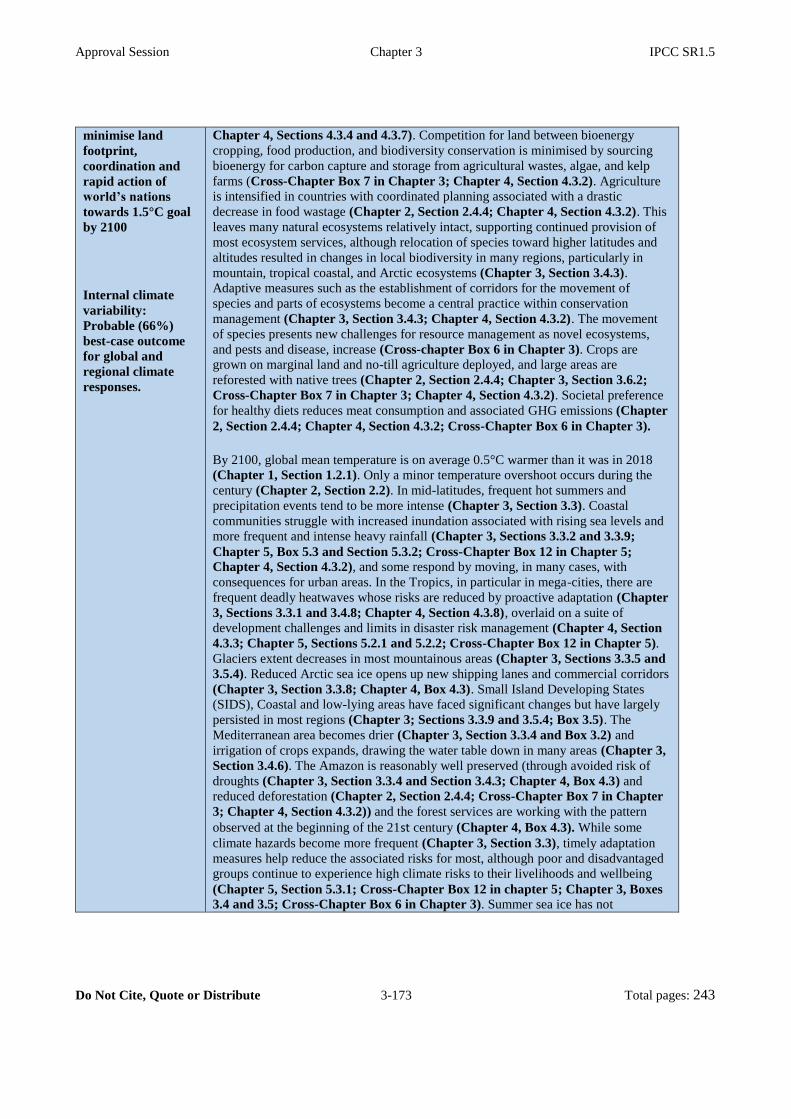
Approval Session Chapter 3 IPCC SR1.5
Do Not Cite, Quote or Distribute 3-173 Total pages: 243
minimise land
footprint,
coordination and
rapid action of
world’s nations
towards 1.5°C goal
by 2100
Internal climate
variability:
Probable (66%)
best-case outcome
for global and
regional climate
responses.
Chapter 4, Sections 4.3.4 and 4.3.7). Competition for land between bioenergy
cropping, food production, and biodiversity conservation is minimised by sourcing
bioenergy for carbon capture and storage from agricultural wastes, algae, and kelp
farms (Cross-Chapter Box 7 in Chapter 3; Chapter 4, Section 4.3.2). Agriculture
is intensified in countries with coordinated planning associated with a drastic
decrease in food wastage (Chapter 2, Section 2.4.4; Chapter 4, Section 4.3.2). This
leaves many natural ecosystems relatively intact, supporting continued provision of
most ecosystem services, although relocation of species toward higher latitudes and
altitudes resulted in changes in local biodiversity in many regions, particularly in
mountain, tropical coastal, and Arctic ecosystems (Chapter 3, Section 3.4.3).
Adaptive measures such as the establishment of corridors for the movement of
species and parts of ecosystems become a central practice within conservation
management (Chapter 3, Section 3.4.3; Chapter 4, Section 4.3.2). The movement
of species presents new challenges for resource management as novel ecosystems,
and pests and disease, increase (Cross-chapter Box 6 in Chapter 3). Crops are
grown on marginal land and no-till agriculture deployed, and large areas are
reforested with native trees (Chapter 2, Section 2.4.4; Chapter 3, Section 3.6.2;
Cross-Chapter Box 7 in Chapter 3; Chapter 4, Section 4.3.2). Societal preference
for healthy diets reduces meat consumption and associated GHG emissions (Chapter
2, Section 2.4.4; Chapter 4, Section 4.3.2; Cross-Chapter Box 6 in Chapter 3).
By 2100, global mean temperature is on average 0.5°C warmer than it was in 2018
(Chapter 1, Section 1.2.1). Only a minor temperature overshoot occurs during the
century (Chapter 2, Section 2.2). In mid-latitudes, frequent hot summers and
precipitation events tend to be more intense (Chapter 3, Section 3.3). Coastal
communities struggle with increased inundation associated with rising sea levels and
more frequent and intense heavy rainfall (Chapter 3, Sections 3.3.2 and 3.3.9;
Chapter 5, Box 5.3 and Section 5.3.2; Cross-Chapter Box 12 in Chapter 5;
Chapter 4, Section 4.3.2), and some respond by moving, in many cases, with
consequences for urban areas. In the Tropics, in particular in mega-cities, there are
frequent deadly heatwaves whose risks are reduced by proactive adaptation (Chapter
3, Sections 3.3.1 and 3.4.8; Chapter 4, Section 4.3.8), overlaid on a suite of
development challenges and limits in disaster risk management (Chapter 4, Section
4.3.3; Chapter 5, Sections 5.2.1 and 5.2.2; Cross-Chapter Box 12 in Chapter 5).
Glaciers extent decreases in most mountainous areas (Chapter 3, Sections 3.3.5 and
3.5.4). Reduced Arctic sea ice opens up new shipping lanes and commercial corridors
(Chapter 3, Section 3.3.8; Chapter 4, Box 4.3). Small Island Developing States
(SIDS), Coastal and low-lying areas have faced significant changes but have largely
persisted in most regions (Chapter 3; Sections 3.3.9 and 3.5.4; Box 3.5). The
Mediterranean area becomes drier (Chapter 3, Section 3.3.4 and Box 3.2) and
irrigation of crops expands, drawing the water table down in many areas (Chapter 3,
Section 3.4.6). The Amazon is reasonably well preserved (through avoided risk of
droughts (Chapter 3, Section 3.3.4 and Section 3.4.3; Chapter 4, Box 4.3) and
reduced deforestation (Chapter 2, Section 2.4.4; Cross-Chapter Box 7 in Chapter
3; Chapter 4, Section 4.3.2)) and the forest services are working with the pattern
observed at the beginning of the 21st century (Chapter 4, Box 4.3). While some
climate hazards become more frequent (Chapter 3, Section 3.3), timely adaptation
measures help reduce the associated risks for most, although poor and disadvantaged
groups continue to experience high climate risks to their livelihoods and wellbeing
(Chapter 5, Section 5.3.1; Cross-Chapter Box 12 in chapter 5; Chapter 3, Boxes
3.4 and 3.5; Cross-Chapter Box 6 in Chapter 3). Summer sea ice has not

Approval Session Chapter 3 IPCC SR1.5
Do Not Cite, Quote or Distribute 3-174 Total pages: 243
completely disappeared from the Arctic (3.4.4.7) and coral reefs having been driven
to a low level (10-30% of levels in 2018) have partially recovered after extensive
dieback by 2100 (Chapter 3, Section 3.4.4.10 and Box 3.4). The Earth system, while
warmer, is still recognizable compared to the 2000s and no major tipping points are
reached (Chapter 3, Section 3.5.2.5). Crop yields remain relatively stable (Chapter
3, Section 3.4). Aggregate economic damage of climate change impacts is relatively
small, although there are some local losses associated with extreme weather events
(Chapter 3, Section 3.5; Chapter 4). Human well-being remains overall similar to
that in 2020 (Chapter 5, Section 5.2.2).
Scenario 2 [one
possible storyline
among mid-case
scenarios]:
Mitigation: Delayed
action (ambitious
targets reached only
after warmer
decade in the 2020s
due to internal
climate variability),
overshoot at 2°C,
decrease towards
1.5°C afterward,
with no efforts to
minimize the land
and water
footprints of
bioenergy.
Internal climate
variability: First,
10% worst-case
outcome (2020s),
then normal
internal climate
variability
The international community continues to largely support the Paris Agreement
and agrees in 2020 on reduction targets for CO2 emissions and time frames for
net-zero emissions. However, these targets are not ambitious enough to reach
stabilization at 2°C warming, let alone 1.5°C.
In the 2020s, internal climate variability leads to higher warming than projected,
in a reverse development to what happened in the so-called “hiatus” period of
the 2000s. Temperatures are regularly above 1.5°C warming although radiative
forcing is consistent with a warming of 1.2°C or 1.3°C. Deadly heatwaves in major
cities (Chicago, Kolkata, Beijing, Karachi, São Paulo), droughts in Southern Europe,
South Africa and the Amazon region, and major flooding in Asia, all intensified by
the global and regional warming (Chapter 3, Sections 3.3.1, 3.3.2, 3.3.3, 3.3.4 and
3.4.8; Chapter 4, Cross-Chapter Box 11 in Chapter 4), lead to increasing levels of
public unrest and political destabilization (Chapter 5, Section 5.2.1). An emergency
global summit in 2025 moves to much more ambitious climate targets. Costs for
rapidly phasing out fossil fuel use and infrastructure, while rapidly expanding
renewables to reduce emissions, are much higher than in Scenario 1 due to a failure to
support economic measures to drive the transition (Chapter 4). Disruptive
technologies become crucial to face up to the adaptation measures needed (Chapter
4, Section 4.4.4).
Temperature peaks at 2°C by the middle of the century before decreasing again due to
intensive implementation of bioenergy plants with carbon capture and storage
(Chapter 2), without efforts to minimize the land and water footprint of the
bioenergy production (Cross-Chapter Box 7 in Chapter 3). Reaching 2°C for
several decades eliminates or severely damages key ecosystems such as coral reefs
and tropical forests (Chapter 3, Section 3.4). The elimination of coral reef
ecosystems and the deterioration of their calcified frameworks, as well as serious
losses of coastal ecosystems such as mangrove forests and seagrass beds (Chapter 3,
Box 3.4, Box 3.5, 3.4.4.10, 3.4.5), leads to much reduced levels of coastal defence
from storms, winds and waves increases the vulnerability and risks facing
communities in tropical and sub-tropical regions with consequences for many coastal
communities (Chapter 5, Cross-Chapter Box 12 in Chapter 5) These impacts are
being amplified by steadily rising sea levels (Chapter 3, Section 3.3.9) and
intensifying storms (Section 3.4.4.3). The intensive area required for the production
of bioenergy combined with increasing water stress sets pressures on food prices
(Cross-Chapter Box 6 in Chapter 3), driving elevated rates of food insecurity,
hunger, and poverty (Chapter 4, Section 4.3.2; Cross-Chaper Box 6 in Chapter 3;
Cross-Chapter Box 11 in Chapter 4). Crop yields decline significantly in the
tropics, leading to prolonged famines in some African countries (Chapter 3, Section

Approval Session Chapter 3 IPCC SR1.5
Do Not Cite, Quote or Distribute 3-175 Total pages: 243
3.4; Chapter 4 Section 4.3.2). Food trumps environment in terms of importance in
most countries with the result that natural ecosystems decrease in abundance due to
climate change as well as of land-use change (Cross-Chapter Box 7 in Chapter
3). The ability to implement adaptive action to prevent the loss of ecosystems is
frustrated under the circumstances and is consequently minimal (Chapter 3, Section
3.4.4.10). Many natural ecosystems, in particular in the Mediterranean, are lost due to
the combined effects of climate change and land use change, and extinction rates
increase greatly (Chapter 3, Section 3.4 and Box 3.2).
By 2100, temperature has decreased but is still higher than 1.5°C, and the yields of
some tropical crops are recovering (Chapter 3, Section 3.4.3). Several of the
remaining natural ecosystems experience irreversible climate-change related damages
whilst others have been lost to land use change, with very rapid increases in the rate
of species extinctions (Chapter 3, Section 3.4; Cross-Chapter Box 7 in Chapter 3;
Chapter 4, Cross-Chapter Box 11 in Chapter 4). Migration, forced displacement,
and loss of identity are extensive in some countries, reversing some achievements in
sustainable development and human security (Chapter 5, Section 5.3.2). Aggregate
economic impacts of climate change damage are small, but the loss in ecosystem
services creates large economic losses (Chapter 4, Sections 4.3.2 and 4.3.3). The
health and well-being of people generally decrease from 2020, while the levels of
poverty and disadvantage increase very significantly (Chapter 5, Section 5.2.1).
Scenario 3 [one
possible storyline
among worst-case
scenarios]:
Mitigation:
Uncoordinated
action, major
actions late in the
21st century, 3°C
warming in 2100.
Internal climate
variability: First
unusual (ca. 10%)
best-case scenario
for one decade, then
normal internal
climate variability
In 2020, despite past pledges, the international support for the Paris Agreement
starts to wane. In the years that follow, CO2 emissions are reduced at local and
national level but efforts are limited and not always successful.
Radiative forcing increases and, due to chance, the most extreme events tend to
happen in less populated regions thus not increasing global concerns. Nonetheless, there are more frequent heatwaves in several cities and less snow in
mountain resorts in the Alps, Rockies, and Andes (Chapter 3, Section 3.3). 1.5°C
warming is reached by 2030, but no major changes in policies occur. Starting with an
intense El Niño-La Niña phase in the 2030s, several catastrophic years occur while
global temperature warming starts to approach 2°C. There are major heatwaves on all
continents, with deadly consequences in tropical regions and Asian megacities,
especially for those ill-equipped for protecting themselves and their communities
from the effects of extreme temperatures (Chapter 3, Sections 3.3.1, 3.3.2 and
3.4.8). Droughts occur in regions bordering the Mediterranean Sea, Central North
America, the Amazon region and southern Australia, some of which are due to
natural variability and others to enhanced greenhouse forcing (Chapter 3, Section
3.3.4; Chapter 4, Section 4.3.2; Cross-Chapter Box 11 in Chapter 4). Intense
floodings occur in high-latitude and tropical regions, in particular in Asia, following
increases in heavy precipitation events (Chapter 3, Section 3.3.3). Major ecosystems
(coral reefs, wetlands, forests) are destroyed over that period (Chapter 3, Section
3.4) with massive disruption to local livelihoods (Chapter 5, Section 5.2.2 and Box
5.3; Cross-Chapter Box 12 in Chapter 5). An unprecedented drought leads to large
impacts on the Amazon rain forest (Chapter 3, Sections 3.3.4 and 3.4), which is also
affected by deforestation (Chapter 2). A hurricane with intense rainfall and
associated with high storm surges (Chapter 3, Section 3.3.6) destroys a large part of
Miami. A 2-year drought in the Great Plains and a concomitant drought in Eastern
Europe and Russia decrease global crop production (Chapter 3, Section 3.3.4),
resulting in major increases in food prices and eroding food security. Poverty levels

Approval Session Chapter 3 IPCC SR1.5
Do Not Cite, Quote or Distribute 3-176 Total pages: 243
increase to a very large scale and risk and incidence of starvation increase very
significantly as food stores dwindle in most countries; human health suffers (Chapter
3, Section 3.4.6.1; Chapter 4, Sections 4.3.2 and 4.4.3; Chapter 5, Section 5.2.1).
There are high levels of public unrest and political destabilization due to the
increasing climatic pressures, resulting in some countries becoming dysfunctional
(Chapter 4, Sections 4.4.1 and 4.4.2). The main countries responsible for the CO2
emissions design rapidly conceived mitigation plans and try to install plants for
carbon capture and storage, in some cases without sufficient prior testing (Chapter 4,
Section 4.3.6). Massive investments in renewable energy often happen too late and
are uncoordinated; energy prices soar as a result of the high demand and lack of
infrastructure. In some cases, demand cannot be met, leading to further delays. Some
countries propose to consider sulphate-aerosol based SRM (Chapter 4, Section
4.3.8), however intensive international negotiations on the topic take substantial time
and are inconclusive, because of overwhelming concerns about potential impacts to
monsoon rainfall and risks in case of termination (Cross-Chapter Box 10 in
Chapter 5). Global and regional temperatures continue to strongly increase while
mitigation solutions are being developed and implemented.
Global mean warming reaches 3°C by 2100 but is not yet stabilized despite major
decreases in yearly CO2 emissions, as a net-zero CO2 emissions budget could not yet
be achieved and because of the long life-time of CO2 concentrations (Chapters 1, 2
and 3). The world as it was in 2020 is no longer recognizable, with decreasing life
expectancy, reduced outdoor labour productivity, and lower quality of life in many
regions because of too frequent heatwaves and other climate extremes (Chapter 4,
Section 4.3.3). Droughts and water resources stress renders agriculture economically
un-viable in some regions (Chapter 3, Section 3.4; Chapter 4, Section 4.3.2) and
contributes to increases in poverty (Chapter 5, Section 5.2.1; Cross-Chapter Box
12 in Chapter 5). Progress on the sustainable development goals is largely undone
and poverty rates reach new highs (Chapter 5, Section 5.2.3). Major conflicts take
place (Chapter 3, Section 3.4.9.6; Chapter 5, Section 5.2.1). Almost all ecosystems
experience irreversible impacts, species extinction rates are high in all regions, forest
fires escalate, and biodiversity strongly decreases, resulting in extensive losses to
ecosystem services. These losses exacerbate poverty and reduce quality of life
(Chapter 3, Section 3.4; Chapter 4, Section 4.3.2). Life, for many indigenous and
rural groups, becomes untenable in their ancestral lands (Chapter 4, Box 4.3;
Chapter 5, Cross-Chapter Box 12 in Chapter 5). The retreat of the West Antarctic
ice sheet accelerates (Chapter 3, Sections 3.3 and 3.6), leading to more rapid SLR
(Chapter 3, Section 3.3.9; Chapter 4, Section 4.3.2). Several small island states
give up hope to survive in their place and look to an increasingly fragmented global
community for refuge (Chapter 3, Box 3.5; Chapter 5, Cross-Chapter Box 12 in
Chapter 5). Aggregate economic damages are substantial owing to the combined
effects of climate changes, political instability, and losses of ecosystem services
(Chapter 4, Sections 4.4.1 and 4.4.2; Chapter 3, Box 3.6 and Section 3.5.2.4). The
general health and well-being of people substantially decreased compared to the
conditions in 2020 and continues to worsen over the following decades (Chapter 5,
Section 5.2.3).
1
2
3

Approval Session Chapter 3 IPCC SR1.5
Do Not Cite, Quote or Distribute 3-177 Total pages: 243
Frequently Asked Questions 1
2
FAQ 3.1: What are the impacts of 1.5°C and 2°C of warming? 3
4 Summary: The impacts of climate change are being felt in every inhabited continent and in the oceans. But 5
they are not spread uniformly across the globe, and different parts of the world experience impacts 6
differently. An average warming of 1.5°C across the whole globe raises the risk of heatwaves and heavy 7
rainfall events, amongst many other potential impacts. Limiting warming to 1.5°C rather than 2°C can help 8
reduce these risks. But the impacts the world experiences will depend on the specific greenhouse gas 9
emission ‘pathway’ taken. The consequences of temporarily overshooting 1.5°C and returning later in the 10
century, for example, could be larger than if temperature stabilizes below 1.5°C. The size and duration of an 11
overshoot will also affect future impacts. 12
13
Human activity has warmed the world by ~1°C since pre-industrial times, and the impacts of this warming 14
are already been felt in many parts of the world. This warming in global temperature is the average of many 15
thousands of temperature measurements taken over the world’s land and oceans. But temperatures aren’t 16
changing at the same speed everywhere. Warming is greatest on continents and is particularly strong in the 17
Arctic in the cold season and mid-latitude regions in the warm season. This is due to self-amplifying 18
mechanisms which increase resulting warming, for instance due to snow and ice melt reducing the 19
reflectivity of solar radiation at the surface, or soil moisture drying leading to less evaporative cooling in the 20
interior of continents. This means that some parts of the world have already experienced temperatures above 21
1.5°C above pre-industrial levels. 22
23
Extra warming on top of the ~1°C we have seen so far would amplify the risks and associated impacts, with 24
implications for the world and its inhabitants. This would be the case even if the total warming is held at 25
1.5°C, just half a degree above where we are now, and would be further amplified at 2°C global warming. 26
Reaching 2°C instead of 1.5°C global warming would lead to substantial warming of extreme hot days in all 27
land regions. It would also lead to an increase in heavy rainfall events in some regions, particularly in the 28
high latitudes of the Northern Hemisphere, potentially raising the risk of flooding. In addition, some regions 29
are projected to become drier at 2°C vs 1.5°C global warming, for example the Mediterranean region. The 30
impacts of any additional warming would also include stronger melting of ice sheets and glaciers, as well as 31
increased sea level rise, which would continue long after the stabilization of atmospheric CO2 32
concentrations. 33
34
Change in climate means and extremes have knock on effects for the societies and ecosystems living on the 35
planet. Climate change is projected to be a poverty multiplier, which means that its impacts make the poor 36
poorer and increase the total number of people living in poverty. The 0.5°C rise in global temperatures that 37
we have experienced in the past 50 years has contributed to shifts in the distribution of plant and animal 38
species, decreasing crop yields and leading to more frequent wildfires. Similar changes can be expected for 39
further rises in global temperature. 40
41
Essentially, the lower the rise in global temperature above preindustrial levels, the lower the risks to human 42
societies and natural ecosystems. Put another way, limiting warming to 1.5°C can be understood in terms of 43
‘avoided impacts’ compared to higher levels of warming. Many of the impacts of climate change assessed in 44
this report have lower associated risks at 1.5°C compared to 2°C. 45
Thermal expansion of the oceans, resulting from the delayed ocean mixing, means sea level will continue to 46
rise even if global temperature is limited to 1.5°C, but this would be lower than in a 2°C world. Ocean 47

Approval Session Chapter 3 IPCC SR1.5
Do Not Cite, Quote or Distribute 3-178 Total pages: 243
acidification, the process by which excess CO2 is dissolving into oceans and making them more acidic, is 1
expected to be less damaging in a world where CO2 emissions are reduced and warming is stabilised at 1.5°C 2
compared to 2°C. The prospect for coral reefs in a 1.5°C world of less damaging than that of a 2ºC world, 3
too. 4
5
The impacts of climate change that we experience in future will also be affected by factors other than the 6
change in temperature. The consequences of 1.5°C warming will additionally depend on the specific 7
greenhouse gas emissions ‘pathway’ that is followed and the extent to which adaptation can reduce 8
vulnerability. This IPCC Special Report uses a number of ‘pathways’ to explore different possibilities for 9
limiting global warming to 1.5°C above preindustrial levels. One type of pathway sees global temperature 10
stabilize at, or just below, 1.5°C. Another sees global temperature temporarily exceed 1.5°C before coming 11
back down later in the century (known as an ‘overshoot’ pathway). 12
13
Such pathways would have different associated impacts, so it is important to distinguish between them for 14
planning adaptation and mitigation strategies. For example, impacts from an overshoot pathway could be 15
larger than impacts from a stabilization pathway. The size and duration of an overshoot would also have 16
consequences for the impacts the world experiences. For example, pathways that overshoot 1.5°C run a 17
greater risk of passing through ‘tipping points’. These are thresholds beyond which certain impacts can no 18
longer be avoided, even if temperatures are brought back down later on. An example is the collapse of the 19
Greenland and Antarctic ice sheets on the time scale of centuries and millennia.20
21 FAQ 3.1, Figure 1: Temperature change is not uniform across the globe. Projected change in average temperature of 22
the annual hottest day (top) and the annual coldest night (bottom) with 1.5°C global warming (left) 23 and 2°C global warming (right) compared to pre-industrial levels. 24
25
Approval Session Chapter 3 IPCC SR1.5
Do Not Cite, Quote or Distribute 3-179 Total pages: 243
References 1
2
Aalto, J., S. Harrison, and M. Luoto, 2017: Statistical modelling predicts almost complete loss of major 3
periglacial processes in Northern Europe by 2100. Nature Communications, 1-8, 4
doi:10.1038/s41467-017-00669-3. 5
Abatzoglou, J.T. and A.P. Williams, 2016: Impact of anthropogenic climate change on wildfire across 6
western US forests. Proceedings of the National Academy of Sciences of the United States of 7
America, 113(42), 11770-11775, doi:10.1073/pnas.1607171113. 8
Abebe, A. et al., 2016: Growth, yield and quality of maize with elevated atmospheric carbon dioxide and 9
temperature in north-west India. Agriculture, Ecosystems & Environment, 218, 66-72, 10
doi:10.1016/j.agee.2015.11.014. 11
Acharya, S.S. and M.K. Panigrahi, 2016: Eastward shift and maintenance of Arabian Sea oxygen minimum 12
zone: Understanding the paradox. Deep-Sea Research Part I: Oceanographic Research Papers, 115, 13
240-252, doi:10.1016/j.dsr.2016.07.004. 14
Adams, C., T. Ide, J. Barnett, and A. Detges, 2018: Sampling bias in climate-conflict research. Nature 15
Climate Change, 8(3), 200-203, doi:10.1038/s41558-018-0068-2. 16
Adger, W.N. et al., 2014: Human Security. In: Climate Change 2014: Impacts, Adaptation, and 17
Vulnerability. Part A: Global and Sectoral Aspects. Contribution of Working Group II to the Fifth 18
Assessment Report of the Intergovernmental Panel on Climate Change [Field, C.B., V.R. Barros, 19
D.J. Dokken, K.J. Mach, M.D. Mastrandrea, T.E. Bilir, M. Chatterjee, K.L. Ebi, Y.O. Estrada, R.C. 20
Genova, B. Girma, E.S. Kissel, A.N. Levy, S. MacCracken, P.R. Mastrandrea, and L.L. White 21
(eds.)]. Cambridge University Press, Cambridge, United Kingdom and New York, NY, USA, pp. 22
755-791. 23
AghaKouchak, A., D. Feldman, M. Hoerling, T. Huxman, and J. Lund, 2015: Water and climate: Recognize 24
anthropogenic drought. Nature, 524(7566), 409-411, doi:10.1038/524409a. 25
Aguilera, R., R. Marcé, and S. Sabater, 2015: Detection and attribution of global change effects on river 26
nutrient dynamics in a large Mediterranean basin. Biogeosciences, 12, 4085-4098, doi:10.5194/bg-27
12-4085-2015. 28
Ahlström, A., G. Schurgers, A. Arneth, and B. Smith, 2012: Robustness and uncertainty in terrestrial 29
ecosystem carbon response to CMIP5 climate change projections. Environmental Research Letters, 30
7(4), 44008. 31
Ahmed, K.F., G. Wang, M. Yu, J. Koo, and L. You, 2015: Potential impact of climate change on cereal crop 32
yield in West Africa. Climatic Change, 133(2), 321-334, doi:10.1007/s10584-015-1462-7. 33
Ainsworth, C.H. et al., 2011: Potential impacts of climate change on Northeast Pacific marine foodwebs and 34
fisheries. ICES Journal of Marine Science, 68(6), 1217-1229. 35
Akbari, H., S. Menon, and A. Rosenfeld, 2009: Global cooling: Increasing world-wide urban albedos to 36
offset CO 2. Climatic Change, 94(3-4), 275-286, doi:10.1007/s10584-008-9515-9. 37
Albert, S. et al., 2017: Heading for the hills: climate-driven community relocations in the Solomon Islands 38
and Alaska provide insight for a 1.5 °C future. Regional Environmental Change, 1-12, 39
doi:10.1007/s10113-017-1256-8. 40
Albright, R. et al., 2016: Ocean acidification: Linking science to management solutions using the Great 41
Barrier Reef as a case study. Journal of Environmental Management, 182, 641-650. 42
Alexander, P. et al., 2017: Assessing uncertainties in land cover projections. Global Change Biology, 23(2), 43
767-781, doi:10.1111/gcb.13447. 44
Alfieri, L., F. Dottori, R. Betts, P. Salamon, and L. Feyen, 2018: Multi-Model Projections of River Flood 45
Risk in Europe under Global Warming. Climate, 6(1)(6). 46
Alfieri, L. et al., 2017: Global projections of river flood risk in a warmer world. Earth's Future, 5(2), 171-47

Approval Session Chapter 3 IPCC SR1.5
Do Not Cite, Quote or Distribute 3-180 Total pages: 243
182, doi:10.1002/2016EF000485. 1
Allen, R., A. Foggo, K. Fabricius, A. Balistreri, and J.M. Hall-Spencer, 2017: Tropical CO 2 seeps reveal the 2
impact of ocean acidification on coral reef invertebrate recruitment. Marine Pollution Bulletin, 3
124(2), 607-613, doi:10.1016/j.marpolbul.2016.12.031. 4
Alongi, D.M., 2008: Mangrove forests: Resilience, protection from tsunamis, and responses to global climate 5
change. Estuarine, Coastal and Shelf Science, 76(1), 1-13, doi:10.1016/j.ecss.2007.08.024. 6
Alongi, D.M., 2015: The Impact of Climate Change on Mangrove Forests. Current Climate Change Reports, 7
1(1), 30-39, doi:10.1007/s40641-015-0002-x. 8
Altieri, A.H. and K.B. Gedan, 2015: Climate change and dead zones. Global Change Biology, 21(4), 1395-9
1406, doi:10.1111/gcb.12754. 10
Altieri, A.H. et al., 2017: Tropical dead zones and mass mortalities on coral reefs. Proceedings of the 11
National Academy of Sciences, 114(14), 3660-3665, doi:10.1073/pnas.1621517114. 12
Alvarez-Filip, L., N.K. Dulvy, J.A. Gill, I.M. Cote, and A.R. Watkinson, 2009: Flattening of Caribbean coral 13
reefs: region-wide declines in architectural complexity. Proceedings of the Royal Society B: 14
Biological Sciences, 276(1669), 3019-3025, doi:10.1098/rspb.2009.0339. 15
Amir, A.K., C. Linyin, M. Omid, and F. Alireza, 2014: Global warming and changes in risk of concurrent 16
climate extremes: Insights from the 2014 California drought. Geophysical Research Letters, 41(24), 17
8847-8852, doi:10.1002/2014GL062308. 18
Anderegg, W.R.L. et al., 2015: Tropical nighttime warming as a dominant driver of variability in the 19
terrestrial carbon sink. Proceedings of the National Academy of Sciences of the United States of 20
America, 112(51), 15591-15596, doi:10.1073/pnas.1521479112. 21
Anderson, K. and G. Peters, 2016: The trouble with negative emissions. Science, 354(6309), 182-183, 22
doi:10.1126/science.aah4567. 23
André, C., D. Boulet, H. Rey-Valette, and B. Rulleau, 2016: Protection by hard defence structures or 24
relocation of assets exposed to coastal risks: Contributions and drawbacks of cost-benefit analysis 25
for long-term adaptation choices to climate change. Ocean and Coastal Management, 134, 173-182, 26
doi:10.1016/j.ocecoaman.2016.10.003. 27
André, G., B. Engel, P.B.M. Berentsen, T.V. Vellinga, and A.G.J.M. Oude Lansink, 2011: Quantifying the 28
effect of heat stress on daily milk yield and monitoring dynamic changes using an adaptive dynamic 29
model. Journal of Dairy Science, 94(9), 4502-4513, doi:10.3168/jds.2010-4139. 30
Anthony, K., 2016: Coral reefs under climate change and ocean acidification: challenges and opportunities 31
for management and policy. Annu. Rev. Environ. Resour., 41, 41:59-81. 32
Anthony, K.R.N. et al., 2015: Operationalizing resilience for adaptive coral reef management under global 33
environmental change. Global Change Biology, 21(1), 48-61, doi:10.1111/gcb.12700. 34
Araos, M. et al., 2016: Climate change adaptation planning in large cities: A systematic global assessment. 35
Environmental Science and Policy, 66, 375-382, doi:10.1016/j.envsci.2016.06.009. 36
Arent, D.J. et al., 2014: Key economic sectors and services. In: Climate Change 2014: Impacts, Adaptation, 37
and Vulnerability. Part A: Global and Sectoral Aspects. Contribution of Working Group II to the 38
Fifth Assessment Report of the Intergovernmental Panel on Climate Change [Field, C.B., V.R. 39
Barros, D.J. Dokken, K.J. Mach, M.D. Mastrandrea, T.E. Bilir, M. Chatterjee, K.L. Ebi, Y.O. 40
Estrada, R.C. Genova, B. Girma, E.S. Kissel, A.N. Levy, S. MacCracken, P.R. Mastrandrea, and 41
L.L. White (eds.)]. Cambridge University Press, Cambridge, United Kingdom and New York, NY, 42
USA, pp. 659-708. 43
Argüeso, D., J.P. Evans, L. Fita, and K.J. Bormann, 2014: Temperature response to future urbanization and 44
climate change. Climate Dynamics, 42(7-8), 2183-2199, doi:10.1007/s00382-013-1789-6. 45
Argüeso, D., J.P. Evans, A.J. Pitman, A. Di Luca, and A. Luca, 2015: Effects of city expansion on heat stress 46
under climate change conditions. PLOS ONE, 10(2), e0117066, doi:10.1371/journal.pone.0117066. 47
Approval Session Chapter 3 IPCC SR1.5
Do Not Cite, Quote or Distribute 3-181 Total pages: 243
Arheimer, B., C. Donnelly, and G. Lindström, 2017: Regulation of snow-fed rivers affects flow regimes 1
more than climate change. Nature Communications, 8(1), 62, doi:10.1038/s41467-017-00092-8. 2
Arias-Ortiz, A. et al., 2018: A marine heatwave drives massive losses from the world's largest seagrass 3
carbon stocks. Nature Climate Change, 8(4), 338-344, doi:10.1038/s41558-018-0096-y. 4
Arkema, K.K. et al., 2013: Coastal habitats shield people and property from sea-level rise and storms. Nature 5
Climate Change, 3(10), 913-918, doi:10.1038/nclimate1944. 6
Armour, K.C., I. Eisenman, E. Blanchard-Wrigglesworth, K.E. McCusker, and C.M. Bitz, 2011: The 7
reversibility of sea ice loss in a state-of-the-art climate model. Geophysical Research Letters, 38(16), 8
doi:10.1029/2011GL048739. 9
Arnell, N.W. and B. Lloyd-Hughes, 2014: The global-scale impacts of climate change on water resources 10
and flooding under new climate and socio-economic scenarios. Climatic Change, 122(1-2), 127-140, 11
doi:10.1007/s10584-013-0948-4. 12
Arnell, N.W., J.A. Lowe, B. Lloyd-Hughes, and T.J. Osborn, 2018: The impacts avoided with a 1.5°C 13
climate target: a global and regional assessment. Climatic Change, 147(1-2), 61-76, 14
doi:10.1007/s10584-017-2115-9. 15
Arnell, N.W. et al., 2016: Global-scale climate impact functions: the relationship between climate forcing 16
and impact. Climatic Change, 134(3), 475-487, doi:10.1007/s10584-013-1034-7. 17
Asiedu, B., J.–O. Adetola, and I. Odame Kissi, 2017a: Aquaculture in troubled climate: Farmers' perception 18
of climate change and their adaptation. Cogent Food & Agriculture, 3(1), 1296400, 19
doi:10.1080/23311932.2017.1296400. 20
Asiedu, B., F.K.E. Nunoo, and S. Iddrisu, 2017b: Prospects and sustainability of aquaculture development in 21
Ghana, West Africa. Cogent Food & Agriculture, 3(1), doi:10.1080/23311932.2017.1349531. 22
Asplund, M.E. et al., 2014: Ocean acidification and host-pathogen interactions: Blue mussels, Mytilus edulis, 23
encountering Vibrio tubiashii. Environmental Microbiology, 16(4), 1029-1039, doi:10.1111/1462-24
2920.12307. 25
Asseng, S. et al., 2013: Uncertainty in simulating wheat yields under climate change. Nature Climate 26
Change, 3(9), 827-832, doi:10.1038/nclimate1916. 27
Asseng, S. et al., 2015: Rising temperatures reduce global wheat production. Nature Climate Change, 5(2), 28
143-147, doi:10.1038/nclimate2470. 29
Atkinson, A., V. Siegel, E.A. Pakhomov, M.J. Jessopp, and V. Loeb, 2009: A re-appraisal of the total 30
biomass and annual production of Antarctic krill. Deep-Sea Research Part I: Oceanographic 31
Research Papers, 56(5), 727-740, doi:10.1016/j.dsr.2008.12.007. 32
Auerbach, L.W. et al., 2015: Flood risk of natural and embanked landscapes on the Ganges-Brahmaputra 33
tidal delta plain. Nature Climate Change, 5, 153-157. 34
Backhaus, A., I. Martinez-Zarzoso, and C. Muris, 2015: Do climate variations explain bilateral migration? A 35
gravity model analysis. IZA Journal of Migration, 4(1), 3, doi:10.1186/s40176-014-0026-3. 36
Bader, D.A. et al., 2018: Urban Climate Science. Climate Change and Cities: Second Assessment Report of 37
the Urban Cliamte Change Research Network, 27-60. 38
Bajželj, B. et al., 2014: Importance of food-demand management for climate mitigation. Nature Climate 39
Change, 4(10), 924-929, doi:10.1038/nclimate2353. 40
Baker, A.C., P.W. Glynn, and B. Riegl, 2008: Climate change and coral reef bleaching: An ecological 41
assessment of long-term impacts, recovery trends and future outlook. Estuarine, Coastal and Shelf 42
Science, 80(4), 435-471, doi:10.1016/j.ecss.2008.09.003. 43
Baker, H.S. et al., 2018: World, Higher CO2 concentrations increase extreme event risk in a 1.5ºC. Nature 44
Climate Change (in press). 45
Bakun, A., 1990: Global climate change and intensification of coastal ocean upwelling. Science, 247(4939), 46
198-201, doi:10.1126/science.247.4939.198. 47

Approval Session Chapter 3 IPCC SR1.5
Do Not Cite, Quote or Distribute 3-182 Total pages: 243
Bakun, A. et al., 2015: Anticipated Effects of Climate Change on Coastal Upwelling Ecosystems. Current 1
Climate Change Reports, 1(2), 85-93, doi:10.1007/s40641-015-0008-4. 2
Baldwin, A. and E. Fornalé, 2017: Adaptive migration: pluralising the debate on climate change and 3
migration. The Geographical Journal, 183(4), 322-328, doi:10.1111/geoj.12242. 4
Barange, M. et al., 2014: Impacts of climate change on marine ecosystem production in societies dependent 5
on fisheries. Nature Climate Change, 4(3), 211-216, doi:10.1038/nclimate2119. 6
Barati, F. et al., 2008: Meiotic competence and DNA damage of porcine oocytes exposed to an elevated 7
temperature. Theriogenology, 69(6), 767-772, doi:10.1016/j.theriogenology.2007.08.038. 8
Barbier, E.B., 2015: Valuing the storm protection service of estuarine and coastal ecosystems. Ecosystem 9
Services, 11, 32-38, doi:10.1016/j.ecoser.2014.06.010. 10
Barnett, J. et al., 2014: A local coastal adaptation pathway. Nature Climate Change, 4(12), 1103-1108, 11
doi:10.1038/nclimate2383. 12
Bassu, S. et al., 2014: How do various maize crop models vary in their responses to climate change factors? 13
Global Change Biology, 20(7), 2301-2320, doi:10.1111/gcb.12520. 14
Bates, N.R. and A.J. Peters, 2007: The contribution of atmospheric acid deposition to ocean acidification in 15
the subtropical North Atlantic Ocean. Marine Chemistry, 107(4), 547-558, 16
doi:10.1016/j.marchem.2007.08.002. 17
Bauer, N. et al., 2018: Global energy sector emission reductions and bioenergy use: overview of the 18
bioenergy demand phase of the EMF 33 model comparison. Climatic Change (in press), 19
doi:doi:10.1007/s10584-018-2226-y. 20
Bayraktarov, E. et al., 2016: The cost and feasibility of marine coastal restoration. Ecological Applications, 21
26(4), 1055-1074, doi:10.1890/15-1077. 22
Bedarff, H. and C. Jakobeit, 2017: Climate change, migration, and displacement. The understimated 23
disaster.. , 38. 24
Bednaršek, N., C.J. Harvey, I.C. Kaplan, R.A. Feely, and J. Možina, 2016: Pteropods on the edge: 25
Cumulative effects of ocean acidification, warming, and deoxygenation. Progress in Oceanography, 26
145, 1-24, doi:10.1016/j.pocean.2016.04.002. 27
Bednaršek, N. et al., 2012: Extensive dissolution of live pteropods in the Southern Ocean. Nature 28
Geoscience, 5(12), 881-885, doi:10.1038/ngeo1635. 29
Bednaršek, N. et al., 2014: Limacina helicina shell dissolution as an indicator of declining habitat suitability 30
owing to ocean acidification in the California Current Ecosystem. Proceedings of the Royal Society 31
B: Biological Sciences, 281(1785), 20140123-20140123, doi:10.1098/rspb.2014.0123. 32
Beetham, E., P.S. Kench, and S. Popinet, 2017: Future Reef Growth Can Mitigate Physical Impacts of Sea-33
Level Rise on Atoll Islands. Earth's Future, 5(10), 1002-1014, doi:10.1002/2017EF000589. 34
Bell, J., 2012: Planning for Climate Change and Sea Level Rise: Queensland's New Coastal Plan. 35
Environmental and Planning Law Journal, 29(1), 61-74. 36
Bell, J. and M. Taylor, 2015: Building Climate-Resilient Food Systems for Pacific Islands. WorldFish, 72. 37
Bell, J.D., J.E. Johnson, and A.J. Hobday, 2011: Vulnerability of tropical pacific fisheries and aquaculture to 38
climate change. 925 pp. 39
Bell, J.D. et al., 2013: Mixed responses of tropical Pacific fisheries and aquaculture to climate change. 40
Nature Climate Change, 3(6), 591-599, doi:10.1038/nclimate1838. 41
Bell, J.D. et al., 2017: Adaptations to maintain the contributions of small-scale fisheries to food security in 42
the Pacific Islands. Marine Policy, doi:10.1016/j.marpol.2017.05.019. 43
Bender, M.A. et al., 2010: Modeled Impact of Anthropogenic Warming on the Frequency of Intense Atlantic 44
Hurricanes. Science, 327(5964), 454-458, doi:10.1126/science.1180568. 45
Benjamini, Y. and Y. Hochberg, 1995: Controlling the False Discovery Rate: A Practical and Powerful 46
Approach to Multiple Testing. Journal of the Royal Statistical Society. Series B (Methodological), 47

Approval Session Chapter 3 IPCC SR1.5
Do Not Cite, Quote or Distribute 3-183 Total pages: 243
57, 289-300, doi:10.2307/2346101. 1
Bertram, C. et al., 2018: Targeted policies can compensate most of the increased sustainability risks in 1.5°C 2
mitigation scenarios. Environmental Research Letters (in press). 3
Bettini, G., 2017: Where Next? Climate Change, Migration, and the (Bio)politics of Adaptation. Global 4
Policy, 8(S1), 33-39, doi:10.1111/1758-5899.12404. 5
Betts, R.A. et al., 2015: Climate and land use change impacts on global terrestrial ecosystems and river flows 6
in the HadGEM2-ES Earth system model using the representative concentration pathways. 7
Biogeosciences, 12(5), 1317-1338, doi:10.5194/bg-12-1317-2015. 8
Betts, R.A. et al., 2018: Changes in climate extremes, fresh water availability and vulnerability to food 9
insecurity projected at 1.5°C and 2°C global warming with a higher-resolution global climate model. 10
Philisophical Transactions Royal Society A, 376(2119), 11
doi:http://dx.doi.org/10.1098/rsta.2016.0452. 12
Beyer, H.L. et al., 2018: Risk-sensitive planning for coral reef conservation under rapid climate change. 13
Conservation Letters, in press. 14
Bichet, A. and A. Diedhiou, 2018: West African Sahel becomes wetter during the last 30 years but dry spells 15
are shorter and more frequent. Climate Research. 16
Bindoff, N.L. et al., 2013a: Detection and Attribution of Climate Change: from Global to Regional. In: 17
Climate Change 2013: The Physical Science Basis. Contribution of Working Group I to the Fifth 18
Assessment Report of the Intergovernmental Panel on Climate Change [Stocker, T.F., D. Qin, G.–K. 19
Plattner, M. Tignor, S.K. Allen, J. Boschung, A. Nauels, Y. Xia, V. Bex, and P.M. Midgley (eds.)]. 20
pp. 867-952. 21
Bindoff, N.L. et al., 2013b: Detection and Attribution of Climate Change: from Global to Regional - 22
Supplementary Material. In: Climate Change 2013: The Physical Science Basis. Contribution of 23
Working Group I to the Fifth Assessment Report of the Intergovernmental Panel on Climate Change 24
[Stocker, T.F., D. Qin, G.–K. Plattner, M. Tignor, S.K. Allen, J. Boschung, A. Nauels, Y. Xia, V. 25
Bex, and P.M. Midgley (eds.)]. pp. 25. 26
Bispo, A. et al., 2017: Accounting for Carbon Stocks in Soils and Measuring GHGs Emission Fluxes from 27
Soils: Do We Have the Necessary Standards? Frontiers in Environmental Science, 5(July), 1-12, 28
doi:10.3389/fenvs.2017.00041. 29
Bittermann, K., S. Rahmstorf, R.E. Kopp, and A.C. Kemp, 2017: Global mean sea-level rise in a world 30
agreed upon in Paris Global mean sea-level rise in a world agreed upon in Paris. Environmental 31
Research Letters. 32
Blankespoor, B., S. Dasgupta, and B. Laplante, 2014: Sea-Level Rise and Coastal Wetlands. AMBIO, 43(8), 33
996-1005, doi:10.1007/s13280-014-0500-4. 34
Block, P. and K. Strzepek, 2012: Power Ahead: Meeting Ethiopia's Energy Needs Under a Changing 35
Climate. Review of Development Economics, 16(3), 476-488, doi:10.1111/j.1467-36
9361.2012.00675.x. 37
Blume-Werry, G., J. Kreyling, H. Laudon, and A. Milbau, 2016: Short-term climate change manipulation 38
effects do not scale up to long-term legacies: effects of an absent snow cover on boreal forest plants. 39
Journal of Ecology, 104(6), 1638-1648, doi:10.1111/1365-2745.12636. 40
Boehlert, B. et al., 2015: Climate change impacts and greenhouse gas mitigation effects on US water quality. 41
Journal of Advances in Modeling Earth Systems, 7(3), 1326-1338, doi:10.1002/2014MS000400. 42
Bonal, D., B. Burban, C. Stahl, F. Wagner, and B. Hérault, 2016: The response of tropical rainforests to 43
drought - lessons from recent research and future prospects. Annals of Forest Science, 73(1), 27-44, 44
doi:10.1007/s13595-015-0522-5. 45
Bongaerts, P., T. Ridgway, E.M. Sampayo, and O. Hoegh-Guldberg, 2010: Assessing the 'deep reef refugia' 46
hypothesis: focus on Caribbean reefs. Coral Reefs, 29(2), 309-327, doi:10.1007/s00338-009-0581-x. 47

Approval Session Chapter 3 IPCC SR1.5
Do Not Cite, Quote or Distribute 3-184 Total pages: 243
Bongaerts, P., C. Riginos, R. Brunner, N. Englebert, and S.R. Smith, 2017: Deep reefs are not universal 1
refuges: reseeding potential varies among coral species. Science Advances, 3(2), e1602373, 2
doi:10.1126/sciadv.1602373. 3
Bonsch, M. et al., 2016: Trade-offs between land and water requirements for large-scale bioenergy 4
production. GCB Bioenergy, 8(1), 11-24, doi:10.1111/gcbb.12226. 5
Bonte, M. and J.J.G. Zwolsman, 2010: Climate change induced salinisation of artificial lakes in the 6
Netherlands and consequences for drinking water production. Water Research, 44(15), 4411-4424, 7
doi:10.1016/j.watres.2010.06.004. 8
Boone, R.B., R.T. Conant, J. Sircely, P.K. Thornton, and M. Herrero, 2017: Impatti sui cambiamenti 9
climatici su determinati servizi ecosistemici di pascoli globali. Biologia del cambiamento globale. 10
Booth, M.S., 2018: Not carbon neutral: Assessing the net emissions impact of residues burned for bioenergy. 11
Environmental Research Letters, 13(3), 035001, doi:10.1088/1748-9326/aaac88. 12
Bopp, L. et al., 2013: Multiple stressors of ocean ecosystems in the 21st century: Projections with CMIP5 13
models. Biogeosciences, 10(10), 6225-6245, doi:10.5194/bg-10-6225-2013. 14
Borma, L.S., C.A. Nobre, and M.F. Cardoso, 2013: 2.15 - Response of the Amazon Tropical Forests to 15
Deforestation, Climate, and Extremes, and the Occurrence of Drought and Fire. Climate 16
Vulnerability, 153-163, doi:10.1016/B978-0-12-384703-4.00228-8. 17
Bosello, F. and E. De Cian, 2014: Climate change, sea level rise, and coastal disasters. A review of modeling 18
practices. Energy Economics, 46, 593-605, doi:10.1016/j.eneco.2013.09.002. 19
Boucher, O. et al., 2012: Reversibility in an Earth System model in response to CO2 concentration changes. 20
Environmental Research Letters, 7(2), doi:10.1088/1748-9326/7/2/024013. 21
Boucher, O. et al., 2013a: Rethinking climate engineering categorization in the context of climate change 22
mitigation and adaptation. WIREs Climate Change, 5(1), 23-35, doi:10.1002/wcc.261. 23
Boucher, O. et al., 2013b: Clouds and Aerosols. In: Climate Change 2013: The Physical Science Basis. 24
Contribution of Working Group I to the Fifth Assessment Report of the Intergovernmental Panel on 25
Climate Change [Stocker, T.F., D. Qin, G.–K. Plattner, M. Tignor, S.K. Allen, J. Boschung, A. 26
Nauels, Y. Xia, V. Bex, and P.M. Midgley (eds.)]. Cambridge University Press, Cambridge, United 27
Kingdom and New York, NY, USA, pp. 573-657. 28
Bouttes, N., J.M. Gregory, and J.A. Lowe, 2013: The Reversibility of Sea Level Rise. Journal of Climate, 29
26(8), 2502-2513, doi:10.1175/JCLI-D-12-00285.1. 30
Bouzid, M., F.J. Colón-González, T. Lung, I.R. Lake, and P.R. Hunter, 2014: Climate change and the 31
emergence of vector-borne diseases in Europe: case study of dengue fever. BMC Public Health, 32
14(1), 781, doi:10.1186/1471-2458-14-781. 33
Boyd, P.W., 2015: Toward quantifying the response of the oceans' biological pump to climate change. 34
Frontiers in Marine Science, 2, doi:10.3389/fmars.2015.00077. 35
Boyd, P.W., S. Sundby, and H.–O. Pörtner, 2014: Cross-chapter box on net primary production in the ocean. 36
In: Climate Change 2014: Impacts, Adaptation, and Vulnerability. Part A: Global and Sectoral 37
Aspects. Contribution of Working Group II to the Fifth Assessment Report of the Intergovernmental 38
Panel of Climate Change [Field, C.B., V.R. Barros, D.J. Dokken, K.J. Mach, M.D. Mastrandrea, 39
T.E. Bilir, M. Chatterjee, K.L. Ebi, Y.O. Estrada, R.C. Genova, B. Girma, E.S. Kissel, A.N. Levy, S. 40
MacCracken, P.R. Mastrandrea, and L.L. White (eds.)]. Cambridge University Press, Cambridge, 41
United Kingdom and New York, NY, USA, pp. 133-136. 42
Boyd, P.W., S.T. Lennartz, D.M. Glover, and S.C. Doney, 2015: Biological ramifications of climate-change-43
mediated oceanic multi-stressors. Nature Climate Change, 5(1), 71-79, doi:10.1038/nclimate2441. 44
Boysen, L. et al., 2017: The limits to global-warming mitigation by terrestrial carbon removal. Earth's 45
Future, 5(5), 463-474, doi:10.1002/2016EF000469. 46
Bozec, Y.–M.M., L. Alvarez-Filip, and P.J. Mumby, 2015: The dynamics of architectural complexity on 47

Approval Session Chapter 3 IPCC SR1.5
Do Not Cite, Quote or Distribute 3-185 Total pages: 243
coral reefs under climate change. Global Change Biology, 21(1), 223-235, doi:10.1111/gcb.12698. 1
Bråthen, K., V. González, and N. Yoccoz, 2018: Gatekeepers to the effects of climate warming? Niche 2
construction restricts plant community changes along a temperature gradient. Perspectives in Plant 3
Ecology, Evolution and Systematics, 30, 71-81, doi:https://doi.org/10.1016/j.ppees.2017.06.005. 4
Breitburg, D. et al., 2018: Declining oxygen in the global ocean and coastal waters. Science, 359(6371), 5
doi:10.1126/science.aam7240. 6
Brigham-Grette, J. et al., 2013: Pliocene Warmth, Polar Amplification, and Stepped Pleistocene Cooling 7
Recorded in NE Arctic Russia. Science, 340(6139), 1421-1427, doi:10.1126/science.1233137. 8
Bright, R.M. et al., 2017: Local temperature response to land cover and management change driven by non-9
radiative processes. Nature Climate Change, 7(4), 296-302, doi:10.1038/nclimate3250. 10
Bring, A. et al., 2016: Arctic terrestrial hydrology: A synthesis of processes, regional effects, and research 11
challenges. Journal of Geophysical Research: Biogeosciences, 121(3), 621-649, 12
doi:10.1002/2015JG003131. 13
Brito, B.P., L.L. Rodriguez, J.M. Hammond, J. Pinto, and A.M. Perez, 2017: Review of the Global 14
Distribution of Foot-and-Mouth Disease Virus from 2007 to 2014. Transboundary and Emerging 15
Diseases, 64(2), 316-332, doi:10.1111/tbed.12373. 16
Brodie, J.E. et al., 2012: Terrestrial pollutant runoff to the Great Barrier Reef: An update of issues, priorities 17
and management responses. Marine Pollution Bulletin, 65(4-9), 81-100, 18
doi:10.1016/j.marpolbul.2011.12.012. 19
Brown, S., R.J. Nicholls, J.A. Lowe, and J. Hinkel, 2016: Spatial variations of sea-level rise and impacts: An 20
application of DIVA. Climatic Change, 134(3), 403-416, doi:10.1007/s10584-013-0925-y. 21
Brown, S. et al., 2018a: Quantifying Land and People Exposed to Sea-Level Rise with No Mitigation and 22
1.5°C and 2.0°C Rise in Global Temperatures to Year 2300. Earth's Future, 6(3), 583-600, 23
doi:10.1002/2017EF000738. 24
Brown, S. et al., 2018b: What are the implications of sea-level rise for a 1.5, 2 and 3 °C rise in global mean 25
temperatures in the Ganges-Brahmaputra-Meghna and other vulnerable deltas? Regional 26
Environmental Change, 1-14, doi:https://doi.org/10.1007/s10113-018-1311-0. 27
28
29
Bruge, A., P. Alvarez, A. Fontán, U. Cotano, and G. Chust, 2016: Thermal Niche Tracking and Future 30
Distribution of Atlantic Mackerel Spawning in Response to Ocean Warming. Frontiers in Marine 31
Science, 3, doi:10.3389/fmars.2016.00086. 32
Bruno, J.F. and E.R. Selig, 2007: Regional decline of coral cover in the Indo-Pacific: Timing, extent, and 33
subregional comparisons. PLoS ONE, 2(8), doi:10.1371/journal.pone.0000711. 34
Brzoska, M. and C. Fröhlich, 2016: Climate change, migration and violent conflict: vulnerabilities, pathways 35
and adaptation strategies. Migration and Development, 5(2), 190-210, 36
doi:10.1080/21632324.2015.1022973. 37
Buhaug, H., 2015: Climate-conflict research: some reflections on the way forward. Wiley Interdisciplinary 38
Reviews: Climate Change, 6(3), 269-275, doi:10.1002/wcc.336. 39
Buhaug, H., 2016: Climate Change and Conflict: Taking Stock. Peace Economics, Peace Science and Public 40
Policy, 22(4), doi:10.1515/peps-2016-0034. 41
Buhaug, H. et al., 2014: One effect to rule them all? A comment on climate and conflict. Climatic Change, 42
127(3-4), 391-397, doi:10.1007/s10584-014-1266-1. 43
Burge, C.A. et al., 2014: Climate Change Influences on Marine Infectious Diseases: Implications for 44
Management and Society. Annual Review of Marine Science, 6(1), 249-277, doi:10.1146/annurev-45
marine-010213-135029. 46
Burke, E.J. et al., 2017: Quantifying uncertainties of permafrost carbon-climate feedbacks. Biogeosciences, 47

Approval Session Chapter 3 IPCC SR1.5
Do Not Cite, Quote or Distribute 3-186 Total pages: 243
14(12), 3051-3066, doi:10.5194/bg-14-3051-2017. 1
Burke, L., K. Reytar, M. Spalding, and A. Perry, 2011: Reefs at risk: Revisited. 115 pp. 2
Burke, M., S.M. Hsiang, and E. Miguel, 2015a: Climate and Conflict. Annual Review of Economics, 7(1), 3
577-617, doi:10.1146/annurev-economics-080614-115430. 4
Burke, M., S.M. Hsiang, and E. Miguel, 2015b: Global non-linear effect of temperature on economic 5
production. Nature, 527(7577), 235-239, doi:10.1038/nature15725. 6
Burke, M., M. Davis, and N. Diffenbaugh, 2018: Large potential reduction in economic damages under UN 7
mitigation targets. Nature (in press). 8
Burrows, K. and P. Kinney, 2016: Exploring the Climate Change, Migration and Conflict Nexus. 9
International Journal of Environmental Research and Public Health, 13(4), 443, 10
doi:10.3390/ijerph13040443. 11
Burrows, M.T. et al., 2014: Geographical limits to species-range shifts are suggested by climate velocity. 12
Nature, 507(7493), 492-495, doi:10.1038/nature12976. 13
Butler, E.E. and P. Huybers, 2013: Adaptation of US maize to temperature variations. Nature Climate 14
Change, 3(1), 68-72, doi:10.1038/nclimate1585. 15
Buurman, J. and V. Babovic, 2016: Adaptation Pathways and Real Options Analysis: An approach to deep 16
uncertainty in climate change adaptation policies. Policy and Society, 35(2), 137-150, 17
doi:10.1016/j.polsoc.2016.05.002. 18
Byers, E. et al., 2018: Global exposure and vulnerability to multi-sector development and climate change 19
hotspots. Environmental Research Letters (in press). 20
Cacciapaglia, C. and R. van Woesik, 2015: Reef-coral refugia in a rapidly changing ocean. Global Change 21
Biology, 21(6), 2272-2282, doi:10.1111/gcb.12851. 22
Caesar, L., S. Rahmstorf, A. Robinson, G. Feulner, and V. Saba, 2018: Observed fingerprint of a weakening 23
Atlantic Ocean overturning circulation. Nature, 556(7700), 191-196, doi:10.1038/s41586-018-0006-24
5. 25
Cai, R., S. Feng, M. Oppenheimer, and M. Pytlikova, 2016: Climate variability and international migration: 26
The importance of the agricultural linkage. Journal of Environmental Economics and Management, 27
79, 135-151, doi:10.1016/j.jeem.2016.06.005. 28
Cai, W. et al., 2012: More extreme swings of the South Pacific convergence zone due to greenhouse 29
warming. Nature, 488, 365. 30
Cai, W. et al., 2015: Increased frequency of extreme La Niña events under greenhouse warming. Nature 31
Climate Change, 5, 132, doi:10.1038/nclimate2492. 32
Cai, W.–J. et al., 2011: Acidification of subsurface coastal waters enhanced by eutrophication. Nature 33
Geoscience, 4(11), 766-770, doi:10.1038/ngeo1297. 34
Cai, Y., T.M. Lenton, and T.S. Lontzek, 2016: Risk of multiple interacting tipping points should encourage 35
rapid CO2 emission reduction. Nature Climate Change, 6(5), 520-525, doi:10.1038/nclimate2964. 36
Caldeira, K., 2013: Coral Bleaching: Coral 'refugia' amid heating seas. Nature Climate Change, 3(5), 444-37
445, doi:10.1038/nclimate1888. 38
Callaway, R. et al., 2012: Review of climate change impacts on marine aquaculture in the UK and Ireland. 39
Aquatic Conservation: Marine and Freshwater Ecosystems, 22(3), 389-421, doi:10.1002/aqc.2247. 40
Camargo, S.J., 2013: Global and Regional Aspects of Tropical Cyclone Activity in the CMIP5 Models. 41
Journal of Climate, 26(24), 9880-9902, doi:10.1175/JCLI-D-12-00549.1. 42
Campbell, J. and O. Warrick, 2014: Climate change and migration issues in the Pacific. United Nations 43
Economic and Social Commission for Asia and the Pacific Pacific Office, 34 pp. 44
Cao, L. and K. Caldeira, 2010: Atmospheric carbon dioxide removal: long-term consequences and 45
commitment. Environmental Research Letters, 5(2), 024011, doi:10.1088/1748-9326/5/2/024011. 46
Cao, L., K. Caldeira, and A.K. Jain, 2007: Effects of carbon dioxide and climate change on ocean 47

Approval Session Chapter 3 IPCC SR1.5
Do Not Cite, Quote or Distribute 3-187 Total pages: 243
acidification and carbonate mineral saturation. Geophysical Research Letters, 34(5), 1
doi:10.1029/2006GL028605. 2
Capo, E. et al., 2017: Tracking a century of changes in microbial eukaryotic diversity in lakes driven by 3
nutrient enrichment and climate warming. Environmental Microbiology, 19(7), 2873-2892, 4
doi:10.1111/1462-2920.13815. 5
Capron, E., A. Govin, R. Feng, B.L. Otto-Bliesner, and E.W. Wolff, 2017: Critical evaluation of climate 6
syntheses to benchmark CMIP6/PMIP4 127 ka Last Interglacial simulations in the high-latitude 7
regions. Quaternary Science Reviews, 168, 137-150, 8
doi:https://doi.org/10.1016/j.quascirev.2017.04.019. 9
Carleton, T., S.M. Hsiang, and M. Burke, 2016: Conflict in a changing climate. The European Physical 10
Journal Special Topics, 225(3), 489-511, doi:10.1140/epjst/e2015-50100-5. 11
Carleton, T.A. and S.M. Hsiang, 2016: Social and economic impacts of climate. Science, 353(6304), 12
aad9837, doi:10.1126/science.aad9837. 13
Carstensen, J., J.H. Andersen, B.G. Gustafsson, and D.J. Conley, 2014: Deoxygenation of the Baltic Sea 14
during the last century. Proceedings of the National Academy of Sciences of the United States of 15
America, 111(15), 5628-33, doi:10.1073/pnas.1323156111. 16
Carter Johnson, W., B. Werner, and G.R. Guntenspergen, 2016: Non-linear responses of glaciated prairie 17
wetlands to climate warming. Climatic Change, 134(1-2), 209-223, doi:10.1007/s10584-015-1534-8. 18
Carvalho, D., A. Rocha, M. Gómez-Gesteira, and C. Silva Santos, 2017: Potential impacts of climate change 19
on European wind energy resource under the CMIP5 future climate projections. Renewable Energy, 20
101, 29-40, doi:10.1016/j.renene.2016.08.036. 21
Castillo, N., L.M. Saavedra, C.A. Vargas, C. Gallardo-Escárate, and C. Détrée, 2017: Ocean acidification 22
and pathogen exposure modulate the immune response of the edible mussel Mytilus chilensis. Fish 23
and Shellfish Immunology, 70, 149-155, doi:10.1016/j.fsi.2017.08.047. 24
Cazenave, A. and G. Cozannet, 2014: Sea level rise and its coastal impacts. Earth's Future, 2(2), 15-34, 25
doi:10.1002/2013EF000188. 26
Cazenave, A. et al., 2014: The rate of sea-level rise. Nature Climate Change, 4(5), 358-361, 27
doi:10.1038/nclimate2159. 28
Ceccarelli, S. and J.E. Rabinovich, 2015: Global Climate Change Effects on Venezuela's Vulnerability to 29
Chagas Disease is Linked to the Geographic Distribution of Five Triatomine Species. Journal of 30
Medical Entomology, 52(6), 1333-1343, doi:10.1093/jme/tjv119. 31
Chadburn, S.E. et al., 2017: An observation-based constraint on permafrost loss as a function of global 32
warming. Nature Climate Change, 1-6, doi:10.1038/nclimate3262. 33
Challinor, A.J. et al., 2014: A meta-analysis of crop yield under climate change and adaptation. Nature 34
Climate Change, 4(4), 287-291, doi:10.1038/nclimate2153. 35
Chapman, A. and S. Darby, 2016: Evaluating sustainable adaptation strategies for vulnerable mega-deltas 36
using system dynamics modelling: Rice agriculture in the Mekong Delta's An Giang Province, 37
Vietnam. Science of the Total Environment, 559, 326-338, doi:10.1016/j.scitotenv.2016.02.162. 38
Chapman, A.D., S.E. Darby, H.M. Hồng, E.L. Tompkins, and T.P.D. Van, 2016: Adaptation and 39
development trade-offs: fluvial sediment deposition and the sustainability of rice-cropping in An 40
Giang Province, Mekong Delta. Climatic Change, 137(3-4), 1-16, doi:10.1007/s10584-016-1684-3. 41
Cheal, A.J., M.A. MacNeil, M.J. Emslie, and H. Sweatman, 2017: The threat to coral reefs from more 42
intense cyclones under climate change. Global Change Biology, 23(4), 1511-1524, 43
doi:10.1111/gcb.13593. 44
Chen, B. et al., 2014: The impact of climate change and anthropogenic activities on alpine grassland over the 45
Qinghai-Tibet Plateau. Agricultural and Forest Meteorology, 189, 11-18, 46
doi:10.1016/j.agrformet.2014.01.002. 47

Approval Session Chapter 3 IPCC SR1.5
Do Not Cite, Quote or Distribute 3-188 Total pages: 243
Chen, C., G.S. Zhou, and L. Zhou, 2014: Impacts of climate change on rice yield in china from 1961 to 2010 1
based on provincial data. Journal of Integrative Agriculture, 13(7), 1555-1564, doi:10.1016/S2095-2
3119(14)60816-9. 3
Chen, J. et al., 2017: Assessing changes of river discharge under global warming of 1.5 °C and 2 °C in the 4
upper reaches of the Yangtze River Basin: Approach by using multiple- GCMs and hydrological 5
models. Quaternary International, 453, 1-11, doi:10.1016/j.quaint.2017.01.017. 6
Cheung, W.W.L., R. Watson, and D. Pauly, 2013: Signature of ocean warming in global fisheries catch. 7
Nature, 497(7449), 365-368, doi:10.1038/nature12156. 8
Cheung, W.W.L., G. Reygondeau, and T.L. Frölicher, 2016a: Large benefits to marine fisheries of meeting 9
the 1.5°C global warming target. Science, 354(6319), 1591-1594, doi:10.1126/science.aag2331. 10
Cheung, W.W.L. et al., 2009: Projecting global marine biodiversity impacts under climate change scenarios. 11
Fish and Fisheries, 10(3), 235-251, doi:10.1111/j.1467-2979.2008.00315.x. 12
Cheung, W.W.L. et al., 2010: Large-scale redistribution of maximum fisheries catch potential in the global 13
ocean under climate change. Global Change Biology, 16(1), 24-35, doi:10.1111/j.1365-14
2486.2009.01995.x. 15
Cheung, W.W.L. et al., 2016b: Structural uncertainty in projecting global fisheries catches under climate 16
change. Ecological Modelling, 325, 57-66, doi:10.1016/j.ecolmodel.2015.12.018. 17
Chiew, F.H.S. et al., 2014: Observed hydrologic non-stationarity in far south-eastern Australia: Implications 18
for modelling and prediction. Stochastic Environmental Research and Risk Assessment, 28(1), 3-15, 19
doi:10.1007/s00477-013-0755-5. 20
Chilkoti, V., T. Bolisetti, and R. Balachandar, 2017: Climate change impact assessment on hydropower 21
generation using multi-model climate ensemble. Renewable Energy, 109, 510-517, 22
doi:10.1016/j.renene.2017.02.041. 23
Cho, S.J. and B.A. McCarl, 2017: Climate change influences on crop mix shifts in the United States. 24
Scientific Reports, 7, 40845, doi:10.1038/srep40845. 25
Chollett, I., P.J. Mumby, and J. Cortés, 2010: Upwelling areas do not guarantee refuge for coral reefs in a 26
warming ocean. Marine Ecology Progress Series, 416, 47-56, doi:10.2307/24875251. 27
Chollett, I., P.J. Mumby, and I.M. Chollett Pj;, 2013: Reefs of last resort: Locating and assessing thermal 28
refugia in the wider Caribbean. Biological Conservation, 167(2013), 179-186, 29
doi:10.1016/j.biocon.2013.08.010. 30
Chollett, I., S. Enr?quez, and P.J. Mumby, 2014: Redefining Thermal Regimes to Design Reserves for Coral 31
Reefs in the Face of Climate Change. PLOS ONE, 9(10), e110634, 32
doi:10.1371/journal.pone.0110634. 33
Christensen, J.H. et al., 2007: Regional Climate Projections. In: Climate Change 2007: The Physical Science 34
Basis. Contribution of Working Group I to the Fourth Assessment Report of the Intergovernmental 35
Panel on Climate Change [Solomon, S., D. Qin, M. Manning, Z. Chen, M. Marquis, K.B. Averyt, 36
M. Tignor, and H.L. Miller (eds.)]. Cambridge University Press, Cambridge, United Kingdom and 37
New York, NY, USA, pp. 847-940. 38
Christensen, J.H. et al., 2013: Climate Phenomena and their Relevance for Future Regional Climate Change. 39
In: Climate Change 2013: The Physical Science Basis. Contribution of Working Group I to the Fifth 40
Assessment Report of the Intergovernmental Panel on Climate Change [Stocker, T.F., D. Qin, G.–K. 41
Plattner, M. Tignor, S.K. Allen, J. Boschung, A. Nauels, Y. Xia, V. Bex, and P.M. Midgley (eds.)]. 42
Cambridge University Press, Cambridge, United Kingdom and New York, NY, USA. 43
Christiansen, S.M., 2016: Introduction. In: Climate Conflicts - A Case of International Environmental and 44
Humanitarian Law. Springer International Publishing, Cham, pp. 1-17. 45
Chung, E.S., H.–K. Cheong, J.–H. Park, J.–H. Kim, and H. Han, 2017: Current and Projected Burden of 46
Disease From High Ambient Temperature in Korea. Epidemiology, 28, S98-S105. 47
Approval Session Chapter 3 IPCC SR1.5
Do Not Cite, Quote or Distribute 3-189 Total pages: 243
Church, J. et al., 2013: Sea level change. Climate Change 2013: The Physical Science Basis. Contribution of 1
Working Group I to the Fifth Assessment Report of the Intergovernmental Panel on Climate Change, 2
1137-1216, doi:10.1017/CB09781107415315.026. 3
Chust, G. et al., 2014a: Biomass changes and trophic amplification of plankton in a warmer ocean. Global 4
Change Biology, 20(7), 2124-2139, doi:10.1111/gcb.12562. 5
Chust, G. et al., 2014b: Are Calanus spp. shifting poleward in the North Atlantic? A habitat modelling 6
approach. ICES Journal of Marine Science, 71(2), 241-253, doi:10.1093/icesjms/fst147. 7
Ciais, P. et al., 2013: Carbon and other biogeochemical cycles. In: Climate Change 2013 the Physical 8
Science Basis: Working Group I Contribution to the Fifth Assessment Report of the 9
Intergovernmental Panel on Climate Change [Stocker, T.F., D. Qin, G.K. Plattner, M. Tignor, S.K. 10
Allen, J. Boschung, A. Nauels, Y. Xia, V. Bex, and P.M. Midgley (eds.)]. Cambridge University 11
Press, Cambridge, United Kingdom and New York, NY, USA, pp. 465-570. 12
Cinner, J.E. et al., 2012: Vulnerability of coastal communities to key impacts of climate change on coral reef 13
fisheries. Global Environmental Change, 22(1), 12-20, doi:10.1016/j.gloenvcha.2011.09.018. 14
Cinner, J.E. et al., 2016: A framework for understanding climate change impacts on coral reef social-15
ecological systems. Regional Environmental Change, 16(4), 1133-1146, doi:10.1007/s10113-015-16
0832-z. 17
Ciscar, J.C. (ed.), 2014: Climate impacts in Europe - The JRC PESETA II project. EUR - Scientific and 18
Technical Research, Publications Office of the European Union. 19
Clark, P.U. et al., 2016: Consequences of twenty-first-century policy for multi-millennial climate and sea-20
level change. Nature Climate Change, 6(4), 360-369, doi:10.1038/NCLIMATE2923. 21
Clarke, L.E. et al., 2014: Assessing Transformation Pathways. In: Climate Change 2014: Mitigation of 22
Climate Change. Contribution of Working Group III to the Fifth Assessment Report of the 23
Intergovernmental Panel on Climate Change [Edenhofer, O., R. Pichs-Madruga, Y. Sokona, E. 24
Farahani, S. Kadner, K. Seyboth, A. Adler, I. Baum, S. Brunner, P. Eickemeier, B. Kriemann, J. 25
Savolainen, S. Schlömer, C. von Stechow, T. Zwickel, and J.C. Minx (eds.)]. Cambridge Univeristy 26
Press, Cambridge, United Kingdom and New York, NY, USA, pp. 413-510. 27
Clausen, K.K. and P. Clausen, 2014: Forecasting future drowning of coastal waterbird habitats reveals a 28
major conservation concern. Biological Conservation, 171, 177-185, 29
doi:10.1016/j.biocon.2014.01.033. 30
Clements, J.C. and T. Chopin, 2017: Ocean acidification and marine aquaculture in North America: Potential 31
impacts and mitigation strategies. Reviews in Aquaculture, 9(4), 326341, doi:10.1111/raq.12140. 32
Clements, J.C., D. Bourque, J. McLaughlin, M. Stephenson, and L.A. Comeau, 2017: Extreme ocean 33
acidification reduces the susceptibility of eastern oyster shells to a polydorid parasite. Journal of 34
Fish Diseases, 40(11), 1573-1585, doi:10.1111/jfd.12626. 35
Collier, R.J. and K.G. Gebremedhin, 2015: Thermal Biology of Domestic Animals. Annual Review of 36
Animal Biosciences, 3(1), 513-532, doi:10.1146/annurev-animal-022114-110659. 37
Collins, M. et al., 2013: Long-term Climate Change: Projections, Commitments and Irreversibility. In: 38
Climate Change 2013: The Physical Science Basis. Contribution of Working Group I to the Fifth 39
Assessment Report of the Intergovernmental Panel on Climate Change [Stocker, T.F., D. Qin, G.–K. 40
Plattner, M. Tignor, S.K. Allen, J. Boschung, A. Nauels, Y. Xia, V. Bex, and P.M. Midgley (eds.)]. 41
Cambridge University Press, Cambridge, United Kingdom and New York, NY, USA, pp. 1029-42
1136. 43
Colón-González, F.J., C. Fezzi, I.R. Lake, P.R. Hunter, and Y. Sukthana, 2013: The Effects of Weather and 44
Climate Change on Dengue. PLoS Neglected Tropical Diseases, 7(11), e2503, 45
doi:10.1371/journal.pntd.0002503. 46
Coniglio, N.D. and G. Pesce, 2015: Climate variability and international migration: an empirical analysis. 47

Approval Session Chapter 3 IPCC SR1.5
Do Not Cite, Quote or Distribute 3-190 Total pages: 243
Environment and Development Economics, 20(04), 434-468, doi:10.1017/S1355770X14000722. 1
Conlon, K., A. Monaghan, M. Hayden, and O. Wilhelmi, 2016: Potential impacts of future warming and land 2
use changes on intra-urban heat exposure in Houston, Texas. PLOS ONE, 11(2), e0148890, 3
doi:10.1371/journal.pone.0148890. 4
Constable, A.L., 2017: Climate change and migration in the Pacific: options for Tuvalu and the Marshall 5
Islands. Regional Environmental Change, 17(4), 1029-1038, doi:10.1007/s10113-016-1004-5. 6
Cook, B.I., M.J. Puma, and N.Y. Krakauer, 2011: Irrigation induced surface cooling in the context of modern 7
and increased greenhouse gas forcing. Climate Dynamics, 37(7-8), 1587-1600, doi:10.1007/s00382-8
010-0932-x. 9
Cook, B.I., K.J. Anchukaitis, R. Touchan, D.M. Meko, and E.R. Cook, 2016: Spatiotemporal drought 10
variability in the Mediterranean over the last 900 years. Journal of Geophysical Research: 11
Atmospheres, 121(5), 2060-2074, doi:10.1002/2015JD023929. 12
Cooper, E.J., 2014: Warmer Shorter Winters Disrupt Arctic Terrestrial Ecosystems. Annual Review of 13
Ecology, Evolution, and Systematics, 45, 271-295, doi:10.1146/annurev-ecolsys-120213-091620. 14
Cooper, J.A.G., M.C. O'Connor, and S. McIvor, 2016: Coastal defences versus coastal ecosystems: A 15
regional appraisal. Marine Policy, doi:10.1016/j.marpol.2016.02.021. 16
Costanza, R. et al., 2014: Changes in the global value of ecosystem services. Global Environmental Change, 17
26(1), 152-158, doi:10.1016/j.gloenvcha.2014.04.002. 18
Coumou, D. and A. Robinson, 2013: Historic and future increase in the global land area affected by monthly 19
heat extremes. Environmental Research Letters, 8(3), 034018, doi:10.1088/1748-9326/8/3/034018. 20
Cousino, L.K., R.H. Becker, and K.A. Zmijewski, 2015: Modeling the effects of climate change on water, 21
sediment, and nutrient yields from the Maumee River watershed. Journal of Hydrology: Regional 22
Studies, 4, 762-775, doi:10.1016/j.ejrh.2015.06.017. 23
Cowtan, K. and R.G. Way, 2014: Coverage bias in the HadCRUT4 temperature series and its impact on 24
recent temperature trends. Quarterly Journal of the Royal Meteorological Society, 140(683), 1935-25
1944, doi:10.1002/qj.2297. 26
Cox, P.M., R.A. Betts, C.D. Jones, S.A. Spall, and I.J. Totterdell, 2000: Acceleration of global warming due 27
to carbon-cycle feedbacks in a coupled climate model. Nature, 408, 184, doi:10.1038/35041539. 28
Cox, P.M. et al., 2013: Sensitivity of tropical carbon to climate change constrained by carbon dioxide 29
variability. Nature, 494, 341, doi:10.1038/nature11882. 30
Craine, J.M., A.J. Elmore, K.C. Olson, and D. Tolleson, 2010: Climate change and cattle nutritional stress. 31
Global Change Biology, 16(10), 2901-2911, doi:10.1111/j.1365-2486.2009.02060.x. 32
Cramer, W. et al., 2014: Detection and Attribution of Observed Impacts. In: Climate Change 2014: Impacts, 33
Adaptation, and Vulnerability. Part A: Global and Sectoral Aspects. Contribution of Working Group 34
II to the Fifth Assessment Report of the Intergovernmental Panel on Climate Change [Field, C.B., 35
V.R. Barros, D.J. Dokken, K.J. Mach, and M.D. Mastrandrea (eds.)]. Cambridge University Press, 36
Cambridge, United Kingdom and New York, NY, USA, pp. 979-1037. 37
Crosby, S.C. et al., 2016: Salt marsh persistence is threatened by predicted sea-level rise. Estuarine, Coastal 38
and Shelf Science, 181, 93-99, doi:https://doi.org/10.1016/j.ecss.2016.08.018. 39
Crowther, T. et al., 2016: Quantifying global soil carbon losses in response to warming. Nature, 540, 104-40
108. 41
Croxall, J.P., 1992: Southern-Ocean Environmental-Changes - Effects on Seabird, Seal and Whale 42
Populations. Philosophical Transactions of the Royal Society of London Series B-Biological 43
Sciences, 338(1285), 319-328, doi:DOI 10.1098/rstb.1992.0152. 44
Cui, L., Z. Ge, L. Yuan, and L. Zhang, 2015: Vulnerability assessment of the coastal wetlands in the Yangtze 45
Estuary, China to sea-level rise. Estuarine, Coastal and Shelf Science, 156(Supplement C), 42-51, 46
doi:https://doi.org/10.1016/j.ecss.2014.06.015. 47

Approval Session Chapter 3 IPCC SR1.5
Do Not Cite, Quote or Distribute 3-191 Total pages: 243
Cunningham, S.C. et al., 2015: Balancing the environmental benefits of reforestation in agricultural regions. 1
Perspectives in Plant Ecology, Evolution and Systematics, 17(4), 301-317, 2
doi:10.1016/j.ppees.2015.06.001. 3
Dai, A., 2016: Historical and Future Changes in Streamflow and Continental Runoff. In: Terrestrial Water 4
Cycle and Climate Change [Tang, Q. and T. Oki (eds.)]. John Wiley & Sons, Inc. pp. 17-37. 5
Daioglou, V. et al., 2016: Projections of the availability and cost of residues from agriculture and forestry. 6
GCB Bioenergy, 8(2), 456-470, doi:10.1111/gcbb.12285. 7
Dale, V.H. et al., 2017: Status and prospects for renewable energy using wood pellets from the southeastern 8
United States. GCB Bioenergy, 9(8), 1296-1305, doi:10.1111/gcbb.12445. 9
Daliakopoulos, I.N. et al., 2017: Yield Response of Mediterranean Rangelands under a Changing Climate. 10
Land Degradation & Development, 28(7), 1962-1972, doi:10.1002/ldr.2717. 11
Dalpadado, P. et al., 2014: Productivity in the Barents Sea - Response to recent climate variability. PLoS 12
ONE, 9(5), e95273, doi:10.1371/journal.pone.0095273. 13
d'Amour, C.B., L. Wenz, M. Kalkuhl, J.C. Steckel, and F. Creutzig, 2016: Teleconnected food supply 14
shocks. Environmental Research Letters, 11(3), 35007. 15
Dargie, G.C. et al., 2017: Age, extent and carbon storage of the central Congo Basin peatland complex. 16
Nature, 542(7639), 86-90, doi:10.1038/nature21048. 17
Dasgupta, P. et al., 2014: Rural areas. In: Climate Change 2014: Impacts, Adaptation, and Vulnerability. 18
Part A: Global and Sectoral Aspects. Contribution of Working Group II to the Fifth Assessment 19
Report of the Intergovernmental Panel on Climate Change [Field, C.B., V.R. Barros, D.J. Dokken, 20
K.J. Mach, M.D. Mastrandrea, T.E. Bilir, M. Chatterjee, K.L. Ebi, Y.O. Estrada, R.C. Genova, B. 21
Girma, E.S. Kissel, A.N. Levy, S. MacCracken, P.R. Mastrandrea, and L.L. White (eds.)]. 22
Cambridge University Press, Cambridge, United Kingdom and New York, NY, USA, pp. 613-657. 23
David, C. et al., 2017: Community structure of under-ice fauna in relation to winter sea-ice habitat properties 24
from the Weddell Sea. Polar Biology, 40(2), 247-261, doi:10.1007/s00300-016-1948-4. 25
Davin, E.L., S.I. Seneviratne, P. Ciais, A. Olioso, and T. Wang, 2014: Preferential cooling of hot extremes 26
from cropland albedo management. Proceedings of the National Academy of Sciences of the United 27
States of America, 111(27), 9757-9761, doi:10.1073/pnas.1317323111. 28
de Jong, J. et al., 2014: Consequences of an increased extraction of forest biofuel in Sweden - A synthesis 29
from the biofuel research programme 2007-2011, supported by Swedish Energy Agency. Summary of 30
the synthesis report. ER 2014:09, Swedish Energy Agency, Eskilstuna, Sweden, 37 pp. 31
de Queiroz, A.R., L.M. Marangon Lima, J.W. Marangon Lima, B.C. da Silva, and L.A. Scianni, 2016: 32
Climate change impacts in the energy supply of the Brazilian hydro-dominant power system. 33
Renewable Energy, 99, 379-389, doi:10.1016/j.renene.2016.07.022. 34
De Rensis, F., I. García-Ispierto, and F. López-Gatius, 2015: Seasonal Heat Stress: Clinical Implications and 35
Hormone Treatments for the Fertility of Dairy Cows. Theriogenology, 84. 36
de Sherbinin, A., 2014: Climate change hotspots mapping: what have we learned? Climatic Change, 123(1), 37
23-37, doi:10.1007/s10584-013-0900-7. 38
De Souza, A.P., J.–C. Cocuron, A.C. Garcia, A.P. Alonso, and M.S. Buckeridge, 2015: Changes in Whole-39
Plant Metabolism during the Grain-Filling Stage in Sorghum Grown under Elevated CO2 and 40
Drought. Plant Physiology, 169(3), 1755 LP - 1765. 41
de Vernal, A., R. Gersonde, H. Goosse, M.–S. Seidenkrantz, and E.W. Wolff, 2013: Sea ice in the 42
paleoclimate system: the challenge of reconstructing sea ice from proxies - an introduction. 43
Quaternary Science Reviews, 79, 1-8, doi:https://doi.org/10.1016/j.quascirev.2013.08.009. 44
de Vrese, P., S. Hagemann, and M. Claussen, 2016: Asian irrigation, African rain: Remote impacts of 45
irrigation. Geophysical Research Letters, 43(8), 3737-3745, doi:10.1002/2016GL068146. 46
De'ath, G., K.E. Fabricius, H. Sweatman, and M. Puotinen, 2012: The 27-year decline of coral cover on the 47

Approval Session Chapter 3 IPCC SR1.5
Do Not Cite, Quote or Distribute 3-192 Total pages: 243
Great Barrier Reef and its causes. Proceedings of the National Academy of Sciences of the United 1
States of America, 109(44), 17995-9, doi:10.1073/pnas.1208909109. 2
DeBeer, C.M., H.S. Wheater, S.K. Carey, and K.P. Chun, 2016: Recent climatic, cryospheric, and 3
hydrological changes over the interior of western Canada: a review and synthesis. Hydrology and 4
Earth System Sciences, 20(4), 1573-1598, doi:10.5194/hess-20-1573-2016. 5
DeConto, R.M. and D. Pollard, 2016: Contribution of Antarctica to past and future sea-level rise. Nature, 6
531(7596), 591-7, doi:10.1038/nature17145. 7
Déqué, M. et al., 2017: A multi-model climate response over tropical Africa at +2°C. Climate Services, 7, 8
87-95, doi:10.1016/j.cliser.2016.06.002. 9
Deryng, D., D. Conway, N. Ramankutty, J. Price, and R. Warren, 2014: Global crop yield response to 10
extreme heat stress under multiple climate change futures. Environmental Research Letters, 9(3), 11
034011, doi:10.1088/1748-9326/9/3/034011. 12
Deutsch, C., A. Ferrel, B. Seibel, H.–O. Pörtner, and R.B. Huey, 2015: Climate change tightens a metabolic 13
constraint on marine habitats. Science, 348(6239), 1132-1135, doi:10.1126/science.aaa1605. 14
Di Lorenzo, E., 2015: Climate science: The future of coastal ocean upwelling. Nature, 518(7539), 310-311, 15
doi:10.1038/518310a. 16
Di Nitto, D. et al., 2014: Mangroves facing climate change: Landward migration potential in response to 17
projected scenarios of sea level rise. Biogeosciences, 11(3), 857-871, doi:10.5194/bg-11-857-2014. 18
Diaz, R.J. and R. Rosenberg, 2008: Spreading Dead Zones and Consequences for Marine Ecosystems. 19
Science, 321(5891), 926-929, doi:10.1126/science.1156401. 20
Diedhiou, A. et al., 2018: Changes in climate extremes over West and Central Africa at 1.5°C and 2°C global 21
warming. Environmental Research Letters (in press). 22
Dieleman, C.M., Z. Lindo, J.W. McLaughlin, A.E. Craig, and B.A. Branfireun, 2016: Climate change effects 23
on peatland decomposition and porewater dissolved organic carbon biogeochemistry. 24
Biogeochemistry, 128(3), 385-396, doi:10.1007/s10533-016-0214-8. 25
Dionisio, K.L. et al., 2017: Characterizing the impact of projected changes in climate and air quality on 26
human exposures to ozone. Journal of Exposure Science And Environmental Epidemiology, 27, 260, 27
doi:10.1038/jes.2016.81. 28
Do, H.X., S. Westra, and M. Leonard, 2017: A global-scale investigation of trends in annual maximum 29
streamflow. Journal of Hydrology, 552, 28-43, doi:10.1016/J.JHYDROL.2017.06.015. 30
Döll, P. et al., 2018: Risks for the global freshwater system at 1.5 °C and 2 °C global warming. 31
Environmental Research Letters, 13(4), 044038, doi:10.1088/1748-9326/aab792. 32
Dolman, A.J. et al., 2010: A Carbon Cycle Science Update Since IPCC AR4. Ambio, 39(5-6), 402-412, 33
doi:10.1007/s13280-010-0083-7. 34
Doney, S., L. Bopp, and M. Long, 2014: Historical and Future Trends in Ocean Climate and 35
Biogeochemistry. Oceanography, 27(1), 108-119, doi:10.5670/oceanog.2014.14. 36
Donk, P., E. Uytven, P. Willems, and M.A. Taylor, 2018: Assessment of the potential implications of a 37
1.5°C versus higher global temperature rise for the Afobaka hydropower scheme in Suriname. 38
Regional Environmental Change, doi:10.1007/s10113-018-1339-1. 39
Donnelly, C. et al., 2017: Impacts of climate change on European hydrology at 1.5, 2 and 3 degrees mean 40
global warming above preindustrial level. Climatic Change, 143(1-2), 13-26, doi:10.1007/s10584-41
017-1971-7. 42
Donner, S.D., 2009: Coping with commitment: Projected thermal stress on coral reefs under different future 43
scenarios. PLoS ONE, 4(6), doi:10.1371/journal.pone.0005712. 44
Donner, S.D., W.J. Skirving, C.M. Little, M. Oppenheimer, and O. Hoegh-Gulberg, 2005: Global assessment 45
of coral bleaching and required rates of adaptation under climate change. Global Change Biology, 46
11(12), 2251-2265, doi:10.1111/j.1365-2486.2005.01073.x. 47

Approval Session Chapter 3 IPCC SR1.5
Do Not Cite, Quote or Distribute 3-193 Total pages: 243
Dosio, A., 2017: Projection of temperature and heat waves for Africa with an ensemble of CORDEX 1
Regional Climate Models. Climate Dynamics, 49(1), 493-519, doi:10.1007/s00382-016-3355-5. 2
Dosio, A. and E.M. Fischer, 2018: Will half a degree make a difference? Robust projections of indices of 3
mean and extreme climate in Europe under 1.5°C, 2°C, and 3°C global warming. Geophys. Res. 4
Lett., 45, 935. 5
Dosio, A., L. Mentaschi, E.M. Fischer, and K. Wyser, 2018: Extreme heat waves under 1.5°C and 2°C 6
global warming. Environmental Research Letters, 13(5), 54006. 7
Dove, S.G. et al., 2013: Future reef decalcification under a business-as-usual CO2 emission scenario. 8
Proceedings of the National Academy of Sciences of the United States of America, 110(38), 15342-9
15347, doi:10.1073/pnas.1302701110. 10
Dowsett, H. et al., 2016: The PRISM4 (mid-Piacenzian) paleoenvironmental reconstruction. Climate of the 11
Past, 12(7), 1519-1538, doi:10.5194/cp-12-1519-2016. 12
Doyon, B., D. Belanger, and P. Gosselin, 2008: The potential impact of climate change on annual and 13
seasonal mortality for three cities in Québec, Canada. International Journal of Health Geographics, 14
7, 23, doi:10.1186/1476-072x-7-23. 15
Draper, F.C. et al., 2014: The distribution and amount of carbon in the largest peatland complex in 16
Amazonia. Environmental Research Letters, 9(12), 124017, doi:10.1088/1748-9326/9/12/124017. 17
Drijfhout, S. et al., 2015: Catalogue of abrupt shifts in Intergovernmental Panel on Climate Change climate 18
models. Proceedings of the National Academy of Sciences of the United States of America, 112(43), 19
E5777-E5786, doi:10.1073/pnas.1511451112. 20
Drouet, A.S. et al., 2013: Grounding line transient response in marine ice sheet models. The Cryosphere, 21
7(2), 395-406, doi:10.5194/tc-7-395-2013. 22
Duarte, C.M. et al., 2013: Is Ocean Acidification an Open-Ocean Syndrome? Understanding Anthropogenic 23
Impacts on Seawater pH. Estuaries and Coasts, 36(2), 221-236, doi:10.1007/s12237-013-9594-3. 24
Duke, N.C. et al., 2017: Large-scale dieback of mangroves in Australia's Gulf of Carpentaria: A severe 25
ecosystem response, coincidental with an unusually extreme weather event. Marine and Freshwater 26
Research, 68(10), 1816-1829, doi:10.1071/MF16322. 27
Dunne, J.P., R.J. Stouffer, and J.G. John, 2013: Reductions in labour capacity from heat stress under climate 28
warming. Nature Climate Change, 3(4), 1-4, doi:10.1038/nclimate1827. 29
Duputié, A., A. Rutschmann, O. Ronce, and I. Chuine, 2015: Phenological plasticity will not help all species 30
adapt to climate change. Global Change Biology, 21(8), 3062-3073, doi:10.1111/gcb.12914. 31
Durack, P.J., S.E. Wijffels, and R.J. Matear, 2012: Ocean Salinities Reveal Strong Global Water Cycle 32
Intensification During 1950 to 2000. Science, 336(6080), 455-458, doi:10.1126/science.1212222. 33
Durand, G. and F. Pattyn, 2015: Reducing uncertainties in projections of Antarctic ice mass loss. The 34
Cryosphere, 9(6), 2043-2055, doi:10.5194/tc-9-2043-2015. 35
Durand, J.–L. et al., 2017: How accurately do maize crop models simulate the interactions of atmospheric 36
CO2 concentration levels with limited water supply on water use and yield? European Journal of 37
Agronomy, doi:https://doi.org/10.1016/j.eja.2017.01.002. 38
Dutton, A. et al., 2015: Sea-level rise due to polar ice-sheet mass loss during past warm periods. Science, 39
349(6244), doi:10.1126/science.aaa4019. 40
Ebi, K.L., N.H. Ogden, J.C. Semenza, and A. Woodward, 2017: Detecting and Attributing Health Burdens to 41
Climate Change. Environmental Health Perspectives, 125(8), 085004, doi:10.1289/EHP1509. 42
Ebi, K.L. et al., 2018: Health risks of warming of 1.5°C, 2°C, and higher, above pre-industrial temperatures. 43
Environmental Research Letters (in press), doi:10.1088/1748-9326/aac4bd. 44
Ekstrom, J.A. et al., 2015: Vulnerability and adaptation of US shellfisheries to ocean acidification. Nature 45
Climate Change, 5(3), 207-214, doi:10.1038/nclimate2508. 46
Elliff, C.I. and I.R. Silva, 2017: Coral reefs as the first line of defense: Shoreline protection in face of climate 47

Approval Session Chapter 3 IPCC SR1.5
Do Not Cite, Quote or Distribute 3-194 Total pages: 243
change. Marine Environmental Research, 127, 148-154, doi:10.1016/j.marenvres.2017.03.007. 1
Elliott, J. et al., 2014: Constraints and potentials of future irrigation water availability on agricultural 2
production under climate change. Proceedings of the National Academy of Sciences, 111(9), 3239-3
3244, doi:10.1073/pnas.1222474110. 4
Ellison, D. et al., 2017: Trees, forests and water: Cool insights for a hot world. Global Environmental 5
Change, 43, 51-61, doi:10.1016/j.gloenvcha.2017.01.002. 6
Ellison, J.C., 2014: Climate Change Adaptation: Management Options for Mangrove Areas. Mangrove 7
Ecosystems of Asia: Status, Challenges and Management Strategies, 391-413, doi:10.1007/978-1-8
4614-8582-7_18. 9
Ellsworth, D.S. et al., 2017: Elevated CO2 does not increase eucalypt forest productivity on a low-10
phosphorus soil. Nature Climate Change, 7, 279, doi:10.1038/nclimate3235. 11
Elsner, J.B., J.P. Kossin, and T.H. Jagger, 2008: The increasing intensity of the strongest tropical cyclones. 12
Nature, 455(7209), 92-95, doi:10.1038/nature07234. 13
Emanuel, K., 2005: Increasing destructiveness of tropical cyclones over the past 30 years. Nature, 436, 686, 14
doi:10.1038/nature03906. 15
Emanuel, K., 2017: A fast intensity simulator for tropical cyclone risk analysis. Natural Hazards, 88(2), 779-16
796, doi:10.1007/s11069-017-2890-7. 17
Endres, S., L. Galgani, U. Riebesell, K.G. Schulz, and A. Engel, 2014: Stimulated bacterial growth under 18
elevated pCO2: Results from an off-shore mesocosm study. PLoS ONE, 9(6), 19
doi:10.1371/journal.pone.0099228. 20
Engelbrecht, C.J. and F.A. Engelbrecht, 2016: Shifts in Köppen-Geiger climate zones over southern Africa 21
in relation to key global temperature goals. Theoretical and Applied Climatology, 123. 22
Engelbrecht, F.A., J.L. McGregor, and C.J. Engelbrecht, 2009: Dynamics of the Conformal-Cubic 23
Atmospheric Model projected climate-change signal over southern Africa. International Journal of 24
Climatology, 29(7), 1013-1033, doi:10.1002/joc.1742. 25
Engelbrecht, F.A. et al., 2015: Projections of rapidly rising surface temperatures over Africa under low 26
mitigation. Environmental Research Letters, 10(8), 085004, doi:10.1088/1748-9326/10/8/085004. 27
Fabricius, K.E. et al., 2011: Losers and winners in coral reefs acclimatized to elevated carbon dioxide 28
concentrations. Nature Climate Change, 1(3), 165-169, doi:10.1038/nclimate1122. 29
Fajardy, M. and N. Mac Dowell, 2017: Can BECCS deliver sustainable and resource efficient negative 30
emissions? Energy & Environmental Science, 10(6), 1389-1426, doi:10.1039/c7ee00465f. 31
Fang, J.K.H., C.H.L. Schönberg, M.A. Mello-Athayde, O. Hoegh-Guldberg, and S. Dove, 2014: Effects of 32
ocean warming and acidification on the energy budget of an excavating sponge. Global Change 33
Biology, 20(4), 1043-1054, doi:10.1111/gcb.12369. 34
Fang, J.K.H. et al., 2013: Sponge biomass and bioerosion rates increase under ocean warming and 35
acidification. Global Change Biology, 19(12), 3581-3591, doi:10.1111/gcb.12334. 36
FAO, 2016: The State of World Fisheries and Aquaculture 2016. Contributing to food security and nutrition 37
for all. Food and Agriculture Organization of the United Nations (FAO), Rome, Italy, 200 pp. 38
FAO, IFAD, UNICEF, WFP, and WHO, 2017: The state of food security and nutrition in the world. Building 39
resilience for peace and food security. Food and Agricultural Organization of the United Nations 40
(FAO), Rome, Italy, 117 pp. 41
Farbotko, C. and H. Lazrus, 2012: The first climate refugees? Contesting global narratives of climate change 42
in Tuvalu. Global Environmental Change, 22(2), 382-390, 43
doi:https://doi.org/10.1016/j.gloenvcha.2011.11.014. 44
Fasullo, J.T., R.S. Nerem, and B. Hamlington, 2016: Is the detection of accelerated sea level rise imminent? 45
Scientific Reports, 6(August), 1-7, doi:10.1038/srep31245. 46
Fawcett, A.A. et al., 2015: Can Paris pledges avert severe climate change? Science, 350(6265), 1168-1169, 47

Approval Session Chapter 3 IPCC SR1.5
Do Not Cite, Quote or Distribute 3-195 Total pages: 243
doi:10.1126/science.aad5761. 1
Faye, B. et al., 2018: Impacts of 1.5 versus 2.0 °C on cereal yields in the West African Sudan Savanna. 2
Environmental Research Letters, 13(3), 34014. 3
Feely, R.A., C.L. Sabine, J.M. Hernandez-Ayon, D. Ianson, and B. Hales, 2008: Evidence for Upwelling of 4
Corrosive "Acidified" Water onto the Continental Shelf. Science, 320(5882), 1490-1492, 5
doi:10.1126/science.1155676. 6
Feely, R.A. et al., 2016: Chemical and biological impacts of ocean acidification along the west coast of 7
North America. Estuarine, Coastal and Shelf Science, 183, 260-270, doi:10.1016/j.ecss.2016.08.043. 8
Feller, I.C., D.A. Friess, K.W. Krauss, and R.R. Lewis, 2017: The state of the world's mangroves in the 21st 9
century under climate change. Hydrobiologia, 803(1), doi:10.1007/s10750-017-3331-z. 10
Feng, X. et al., 2016: Revegetation in China's Loess Plateau is approaching sustainable water resource limits. 11
Nature Climate Change, 6(11), 1019-1022, doi:10.1038/nclimate3092. 12
Ferrario, F. et al., 2014: The effectiveness of coral reefs for coastal hazard risk reduction and adaptation. 13
Nature Communications, 5, 3794, doi:10.1038/ncomms4794. 14
Fine, M., H. Gildor, and A. Genin, 2013: A coral reef refuge in the Red Sea. Global Change Biology, 19(12), 15
3640-3647, doi:10.1111/gcb.12356. 16
Fischer, D., S.M. Thomas, F. Niemitz, B. Reineking, and C. Beierkuhnlein, 2011: Projection of climatic 17
suitability for Aedes albopictus Skuse (Culicidae) in Europe under climate change conditions. 18
Global and Planetary Change, 78(1-2), 54-64, doi:10.1016/j.gloplacha.2011.05.008. 19
Fischer, D. et al., 2013: Climate change effects on Chikungunya transmission in Europe: geospatial analysis 20
of vector's climatic suitability and virus' temperature requirements. International Journal of Health 21
Geographics, 12(1), 51, doi:10.1186/1476-072X-12-51. 22
Fischer, E.M. and R. Knutti, 2015: Anthropogenic contribution to global occurrence of heavy-precipitation 23
and high-temperature extremes. Nature Climate Change, 5(6), 560-564, doi:10.1038/nclimate2617. 24
Fischer, E.M., J. Sedláček, E. Hawkins, and R. Knutti, 2014: Models agree on forced response pattern of 25
precipitation and temperature extremes. Geophysical Research Letters, 41(23), 8554-8562, 26
doi:10.1002/2014GL062018. 27
Fischer, H. et al., 2018: Paleoclimate constraints on a future warmer world. Science (in press). 28
Ford, J.D., 2012: Indigenous health and climate change. American Journal of Public Health, 102(7), 1260-29
1266, doi:10.2105/AJPH.2012.300752. 30
Ford, J.D., G. McDowell, and T. Pearce, 2015: The adaptation challenge in the Arctic. Nature Climate 31
Change, 5(12), 1046-1053, doi:10.1038/nclimate2723. 32
Forseth, I., 2010: Terrestrial Biomes. Nature Education Knowledge, 3(10), 11. 33
Fossheim, M. et al., 2015: Recent warming leads to a rapid borealization of fish communities in the Arctic. 34
Nature Climate Change, 5(7), 673-677, doi:10.1038/nclimate2647. 35
Fox, N.J. et al., 2011: Predicting Impacts of Climate Change on Fasciola hepatica Risk. PLoS ONE, 6(1), 36
e16126, doi:10.1371/journal.pone.0016126. 37
Frank, D.C. et al., 2010: Ensemble reconstruction constraints on the global carbon cycle sensitivity to 38
climate. Nature, 463, 527. 39
Fricko, O. et al., 2016: Energy sector water use implications of a 2 °C climate policy. Environmental 40
Research Letters, 11(3), 034011, doi:10.1088/1748-9326/11/3/034011. 41
Frieler, K. et al., 2013: Limiting global warming to 2C is unlikely to save most coral reefs. Nature Climate 42
Change, 3(2), 165-170, doi:10.1038/nclimate1674. 43
Frieler, K. et al., 2015: Consistent evidence of increasing Antarctic accumulation with warming. Nature 44
Climate Change, 5(4), 348-352. 45
Frieler, K. et al., 2017: Assessing the impacts of 1.5°C global warming - simulation protocol of the Inter-46
Sectoral Impact Model Intercomparison Project (ISIMIP2b). Geoscientific Model Development, 10, 47

Approval Session Chapter 3 IPCC SR1.5
Do Not Cite, Quote or Distribute 3-196 Total pages: 243
4321-4345, doi:10.5194/gmd-10-4321-2017. 1
Friend, A.D. et al., 2014: Carbon residence time dominates uncertainty in terrestrial vegetation responses to 2
future climate and atmospheric CO2. Proceedings of the National Academy of Sciences, 111(9), 3
3280-3285, doi:10.1073/pnas.1222477110. 4
Fronzek, S., T.R. Carter, and M. Luoto, 2011: Evaluating sources of uncertainty in modelling the impact of 5
probabilistic climate change on sub-arctic palsa mires. Natural Hazards and Earth System Science, 6
11(11), 2981-2995, doi:10.5194/nhess-11-2981-2011. 7
Frost, A.J. et al., 2011: A comparison of multi-site daily rainfall downscaling techniques under Australian 8
conditions. Journal of Hydrology, 408(1), 1-18, doi:10.1016/j.jhydrol.2011.06.021. 9
Fu, X. and J. Song, 2017: Assessing the economic costs of sea level rise and benefits of coastal protection: A 10
spatiotemporal approach. Sustainability, 9(8), doi:10.3390/su9081495. 11
Fuerst, J.J., H. Goelzer, and P. Huybrechts, 2015: Ice-dynamic projections of the Greenland ice sheet in 12
response to atmospheric and oceanic warming. The Cryosphere, 9(3), 1039-1062, doi:10.5194/tc-9-13
1039-2015. 14
Fuss, S. et al., 2014: Betting on negative emissions. Nature Climate Change, 4(10), 850-853, 15
doi:10.1038/nclimate2392. 16
Fuss, S. et al., 2018: Negative emissions - Part 2: Costs, potentials and side effects. Environmental Research 17
Letters (in press). 18
Gagne, M.–E., J.C. Fyfe, N.P. Gillett, I. Polyakov, and G.M. Flato, 2017: Aerosol-driven increase in Arctic 19
sea ice over the middle of the twentieth century. Geophysical Research Letters, 44(14), 7338-7346, 20
doi:10.1002/2016GL071941. 21
Galaasen, E.V. et al., 2014: Rapid Reductions in North Atlantic Deep Water During the Peak of the Last 22
Interglacial Period. Science, 343(6175), 1129-1132, doi:10.1126/science.1248667. 23
Gang, C. et al., 2015: Projecting the dynamics of terrestrial net primary productivity in response to future 24
climate change under the RCP2.6 scenario. Environmental Earth Sciences, 74(7), 5949-5959, 25
doi:10.1007/s12665-015-4618-x. 26
García Molinos, J. et al., 2015: Climate velocity and the future global redistribution of marine biodiversity. 27
Nature Climate Change, 6(1), 83-88, doi:10.1038/nclimate2769. 28
Gardner, T.A., I.M. Côté, J.A. Gill, A. Grant, and A.R. Watkinson, 2005: Hurricanes and caribbean coral 29
reefs: Impacts, recovery patterns, and role in long-term decline. Ecology, 86(1), 174-184, 30
doi:10.1890/04-0141. 31
Garland, R.M. et al., 2015: Regional Projections of Extreme Apparent Temperature Days in Africa and the 32
Related Potential Risk to Human Health. International Journal of Environmental Research and 33
Public Health, 12(10), 12577-12604, doi:10.3390/ijerph121012577. 34
Garrabou, J. et al., 2009: Mass mortality in Northwestern Mediterranean rocky benthic communities: Effects 35
of the 2003 heat wave. Global Change Biology, 15(5), 1090-1103, doi:10.1111/j.1365-36
2486.2008.01823.x. 37
Garrard, S.L. et al., 2014: Indirect effects may buffer negative responses of seagrass invertebrate 38
communities to ocean acidification. Journal of Experimental Marine Biology and Ecology, 461, 31-39
38, doi:10.1016/j.jembe.2014.07.011. 40
Gasparrini, A. et al., 2015: Mortality risk attributable to high and low ambient temperature: A multicountry 41
observational study. The Lancet, 386(9991), 369-375, doi:10.1016/S0140-6736(14)62114-0. 42
Gass, P., H. Hove, and P. Jo-Ellen, 2011: Review of Current and Planned Adaptation Action: East and 43
Southeast Asia. 230 pp. 44
Gattuso, J.–P. et al., 2015: Contrasting futures for ocean and society from different anthropogenic CO2 45
emissions scenarios. Science, 349(6243), aac4722, doi:10.1126/science.aac4722. 46
Gatusso, J.–P. et al., 2014: Cross-chapter box on ocean acidification. In: Climate Change 2014: Impacts, 47

Approval Session Chapter 3 IPCC SR1.5
Do Not Cite, Quote or Distribute 3-197 Total pages: 243
Adaptation, and Vulnerability. Part A: Global and Sectoral Aspects. Contribution of Working Group 1
II to the Fifth Assessment Report of the Intergovernmental Panel of Climate Change [Field, C.B., 2
V.R. Barros, D.J. Dokken, K.J. Mach, M.D. Mastrandrea, T.E. Bilir, M. Chatterjee, K.L. Ebi, Y.O. 3
Estrada, R.C. Genova, B. Girma, E.S. Kissel, A.N. Levy, S. MacCracken, P.R. Mastrandrea, and 4
L.L. White (eds.)]. Cambridge University Press, Cambridge, United Kingdom and New York, NY, 5
USA, pp. 129-131. 6
Gauthier, S., P. Bernier, T. Kuuluvainen, A.Z. Shvidenko, and D.G. Schepaschenko, 2015: Boreal forest 7
health and global change. Science, 349(6250), 819-822, doi:10.1126/science.aaa9092. 8
Geisler, C. and B. Currens, 2017: Impediments to inland resettlement under conditions of accelerated sea 9
level rise. Land Use Policy, 66, 322-330. 10
Georgescu, M., M. Moustaoui, A. Mahalov, and J. Dudhia, 2012: Summer-time climate impacts of projected 11
megapolitan expansion in Arizona. Nature Climate Change, 3(1), 37-41, doi:10.1038/nclimate1656. 12
Gerten, D., S. Rost, W. von Bloh, and W. Lucht, 2008: Causes of change in 20th century global river 13
discharge. Geophysical Research Letters, 35(20), L20405, doi:10.1029/2008GL035258. 14
Gerten, D. et al., 2013: Asynchronous exposure to global warming: freshwater resources and terrestrial 15
ecosystems. Environmental Research Letters, 8(3), 034032, doi:10.1088/1748-9326/8/3/034032. 16
Gharbaoui, D. and J. Blocher, 2016: The Reason Land Matters: Relocation as Adaptation to Climate Change 17
in Fiji Islands. Migration, Risk Management and Climate Change: Evidence and Policy Responses, 18
149-173, doi:10.1007/978-3-319-42922-9_8. 19
Ghosh, J., 2010: The unnatural coupling: Food and global finance. Journal of Agrarian Change, 10(1), 72-20
86, doi:10.1111/j.1471-0366.2009.00249.x. 21
Giardino, A., K. Nederhoff, and M. Vousdukas, 2018: Coastal hazard risk assessment for small islands: 22
assessing the impact of climate change and disaster reduction measures on Ebeye (Marshall Islands). 23
Regional Environmental Change, 1-12, doi:DOI: 10.1007/s10113-018-1353-3. 24
Goddard, P.B., C.O. Dufour, J. Yin, S.M. Griffies, and M. Winton, 2017: CO2-Induced Ocean Warming of 25
the Antarctic Continental Shelf in an Eddying Global Climate Model. Journal of Geophysical 26
Research - Oceans, 122(10), 8079-8101, doi:10.1002/2017JC012849. 27
Goll, D.S. et al., 2012: Nutrient limitation reduces land carbon uptake in simulations with a model of 28
combined carbon, nitrogen and phosphorus cycling. Biogeosciences, 9(9), 3547-3569, 29
doi:10.5194/bg-9-3547-2012. 30
Golledge, N.R. et al., 2015: The multi-millennial Antarctic commitment to future sea-level rise. Nature, 31
526(7573), 421-425, doi:10.1038/nature15706. 32
González, C., A. Paz, and C. Ferro, 2014: Predicted altitudinal shifts and reduced spatial distribution of 33
Leishmania infantum vector species under climate change scenarios in Colombia. Acta Tropica, 129, 34
83-90, doi:10.1016/j.actatropica.2013.08.014. 35
Good, P., C. Jones, J. Lowe, R. Betts, and N. Gedney, 2013: Comparing Tropical Forest Projections from 36
Two Generations of Hadley Centre Earth System Models, HadGEM2-ES and HadCM3LC. Journal 37
of Climate, 26(2), 495-511, doi:10.1175/JCLI-D-11-00366.1. 38
Good, P. et al., 2011: Quantifying Environmental Drivers of Future Tropical Forest Extent. Journal of 39
Climate, 24(5), 1337-1349, doi:10.1175/2010JCLI3865.1. 40
Goodwin, P., I.D. Haigh, E.J. Rohling, and A. Slangen, 2017: A new approach to projecting 21st century 41
sea-level changes and extremes. Earth's Future, 5(2), 240-253, doi:10.1002/2016EF000508. 42
Goodwin, P., S. Brown, I.D. Haigh, R.J. Nicholls, and J.M. Matter, 2018: Adjusting Mitigation Pathways to 43
Stabilize Climate at 1.5°C and 2.0°C Rise in Global Temperatures to Year 2300. Earth's Future, 44
6(3), 601-615, doi:10.1002/2017EF000732. 45
Gosling, S.N. and N.W. Arnell, 2016: A global assessment of the impact of climate change on water scarcity. 46
Climatic Change, 134(3), 371-385, doi:10.1007/s10584-013-0853-x. 47

Approval Session Chapter 3 IPCC SR1.5
Do Not Cite, Quote or Distribute 3-198 Total pages: 243
Gosling, S.N. et al., 2017: A comparison of changes in river runoff from multiple global and catchment-scale 1
hydrological models under global warming scenarios of 1°C, 2°C and 3°C. Climatic Change, 141(3), 2
577-595, doi:10.1007/s10584-016-1773-3. 3
Graham, N.A.J., 2014: Habitat complexity: Coral structural loss leads to fisheries declines. Current Biology, 4
24(9), R359-R361, doi:10.1016/j.cub.2014.03.069. 5
Graham, N.A.J., S. Jennings, M.A. MacNeil, D. Mouillot, and S.K. Wilson, 2015: Predicting climate-driven 6
regime shifts versus rebound potential in coral reefs. Nature, 518(7537), 1-17, 7
doi:10.1038/nature14140. 8
Graux, A.–I., G. Bellocchi, R. Lardy, and J.–F. Soussana, 2013: Ensemble modelling of climate change risks 9
and opportunities for managed grasslands in France. Agricultural and Forest Meteorology, 170, 114-10
131, doi:10.1016/j.agrformet.2012.06.010. 11
Green, A.L. et al., 2014: Designing Marine Reserves for Fisheries Management, Biodiversity Conservation, 12
and Climate Change Adaptation. Coastal Management, 42(2), 143-159, 13
doi:10.1080/08920753.2014.877763. 14
Gregory, J.M. and P. Huybrechts, 2006: Ice-sheet contributions to future sea-level change. Philosophical 15
Transactions of the Royal Society of London A: Mathematical, Physical and Engineering Sciences, 16
364(1844), 1709-1731, doi:10.1098/rsta.2006.1796. 17
Gregory, P.J. and B. Marshall, 2012: Attribution of climate change: a methodology to estimate the potential 18
contribution to increases in potato yield in Scotland since 1960. Global Change Biology, 18(4), 19
1372-1388, doi:10.1111/j.1365-2486.2011.02601.x. 20
Greve, P. and S.I. Seneviratne, 2015: Assessment of future changes in water availability and aridity. 21
Geophysical Research Letters, 42(13), 5493-5499, doi:10.1002/2015GL064127. 22
Greve, P., L. Gudmundsson, and S.I. Seneviratne, 2018: Regional scaling of annual mean precipitation and 23
water availability with global temperature change. Earth System Dynamics, 9(1), 227-240, 24
doi:10.5194/esd-9-227-2018. 25
Greve, P. et al., 2014: Global assessment of trends in wetting and drying over land. Nature Geoscience, 26
7(10), 716-721, doi:10.1038/ngeo2247. 27
Grillakis, M.G., A.G. Koutroulis, K.D. Seiradakis, and I.K. Tsanis, 2016: Implications of 2 °C global 28
warming in European summer tourism. Climate Services, 1, 30-38, doi:10.1016/j.cliser.2016.01.002. 29
Grillakis, M.G., A.G. Koutroulis, I.N. Daliakopoulos, and I.K. Tsanis, 2017: A method to preserve trends in 30
quantile mapping bias correction of climate modeled temperature. Earth System Dynamics, 8, 889-31
900, doi:10.5194/esd-8-889-2017. 32
Griscom, B.W. et al., 2017: Natural climate solutions. Proceeding of the National Academy of Sciences of 33
the United States of America, 114(44), 11645-11650, doi:10.1073/pnas.1710465114. 34
Grossman-Clarke, S., S. Schubert, and D. Fenner, 2017: Urban effects on summertime air temperature in 35
Germany under climate change. International Journal of Climatology, 37(2), 905-917, 36
doi:10.1002/joc.4748. 37
Grübler, A., 2018: A Global Scenario of Low Energy Demand for Sustainable Development below 1.5°C 38
without Negative Emission Technologies. (in press). 39
Gu, G. and R.F. Adler, 2013: Interdecadal variability/long-term changes in global precipitation patterns 40
during the past three decades: global warming and/or pacific decadal variability? Climate Dynamics, 41
40(11-12), 3009-3022, doi:10.1007/s00382-012-1443-8. 42
Gu, G. and R.F. Adler, 2015: Spatial patterns of global precipitation change and variability during 1901-43
2010. Journal of Climate, 28(11), 4431-4453, doi:10.1175/JCLI-D-14-00201.1. 44
Gudmundsson, L. and S.I. Seneviratne, 2016: Anthropogenic climate change affects meteorological drought 45
risk in Europe. Environmental Research Letters, 11(4), 044005, doi:10.1088/1748-46
9326/11/4/044005. 47

Approval Session Chapter 3 IPCC SR1.5
Do Not Cite, Quote or Distribute 3-199 Total pages: 243
Gudmundsson, L., S.I. Seneviratne, and X. Zhang, 2017: Anthropogenic climate change detected in 1
European renewable freshwater resources. Nature Climate Change, 7, 813. 2
Guiot, J. and W. Cramer, 2016: Climate change: The 2015 Paris Agreement thresholds and Mediterranean 3
basin ecosystems. Science, 354(6311), 4528-4532, doi:10.1126/science.aah5015. 4
Guis, H. et al., 2012: Modelling the effects of past and future climate on the risk of bluetongue emergence in 5
Europe. Journal of The Royal Society Interface, 9(67), 339-350, doi:10.1098/rsif.2011.0255. 6
Guo, Y. et al., 2016: Projecting future temperature-related mortality in three largest Australian cities. 7
Environmental Pollution, 208(January 2016), 66-73, doi:10.1016/j.envpol.2015.09.041. 8
Gupta, H., S.–J. Kao, and M. Dai, 2012: The role of mega dams in reducing sediment fluxes: A case study of 9
large Asian rivers. Journal of Hydrology, 464-465(Supplement C), 447-458, 10
doi:https://doi.org/10.1016/j.jhydrol.2012.07.038. 11
Gustafson, S., A. Joehl Cadena, and P. Hartman, 2016: Adaptation planning in the Lower Mekong Basin: 12
merging scientific data with local perspective to improve community resilience to climate change. 13
Climate and Development, 1-15, doi:10.1080/17565529.2016.1223593. 14
Gustafson, S. et al., 2017: Merging science into community adaptation planning processes: a cross-site 15
comparison of four distinct areas of the Lower Mekong Basin. Climatic Change, 16
doi:10.1007/s10584-016-1887-7. 17
Gutiérrez, J.L. et al., 2012: Physical Ecosystem Engineers and the Functioning of Estuaries and Coasts. 18
Treatise on Estuarine and Coastal Science, 7, 53-81, doi:10.1016/B978-0-12-374711-2.00705-1. 19
Haberl, H., T. Beringer, S.C. Bhattacharya, K.–H. Erb, and M. Hoogwijk, 2010: The global technical 20
potential of bio-energy in 2050 considering sustainability constraints. Current Opinion in 21
Environmental Sustainability, 2(5), 394-403, doi:https://doi.org/10.1016/j.cosust.2010.10.007. 22
Haberl, H. et al., 2013: Bioenergy: how much can we expect for 2050? Environmental Research Letters, 23
8(3), 31004. 24
Habibi Mohraz, M., A. Ghahri, M. Karimi, and F. Golbabaei, 2016: The Past and Future Trends of Heat 25
Stress Based On Wet Bulb Globe Temperature Index in Outdoor Environment of Tehran City, Iran. 26
Iranian Journal of Public Health, 45(6), 787-794. 27
Hadden, D. and A. Grelle, 2016: Changing temperature response of respiration turns boreal forest from 28
carbon sink into carbon source. Agricultural and Forest Meteorology, 29
doi:10.1016/j.agrformet.2016.03.020. 30
Hajat, S., S. Vardoulakis, C. Heaviside, and B. Eggen, 2014: Climate change effects on human health: 31
Projections of temperature-related mortality for the UK during the 2020s, 2050s and 2080s. Journal 32
of Epidemiology and Community Health, 68(7), 641-648, doi:10.1136/jech-2013-202449. 33
Hales, S., S. Kovats, S. Lloyd, and D. Campbell-Lendrum (eds.), 2014: Quantitative risk assessment of the 34
effects of climate change on selected causes of death, 2030s and 2050s. World Health Organization 35
(WHO), Geneva, Switzerland, 115 pp. 36
Hall, J. et al., 2014: Understanding flood regime changes in Europe: a state-of-the-art assessment. Hydrology 37
and Earth System Sciences, 18(7), 2735-2772, doi:10.5194/hess-18-2735-2014. 38
Hallegatte, S. and J. Rozenberg, 2017: Climate change through a poverty lens. Nature Climate Change, 7(4), 39
250-256, doi:10.1038/nclimate3253. 40
Hallegatte, S., C. Green, R. J. Nicholls, and J. Corfee-Morlot, 2013: Future flood losses in major coastal 41
cities. Nature Climate Change, 3, 802-806. 42
Hallegatte, S. et al., 2016: Shock Waves: Managing the Impacts of Climate Change on Poverty. , 227. 43
Hall-Spencer, J.M. et al., 2008: Volcanic carbon dioxide vents show ecosystem effects of ocean 44
acidification. Nature, 454(7200), 96-99, doi:10.1038/nature07051. 45
Halpern, B.S. et al., 2015: Spatial and temporal changes in cumulative human impacts on the world's ocean. 46
Nature Communications, 6, 7615, doi:10.1038/ncomms8615. 47

Approval Session Chapter 3 IPCC SR1.5
Do Not Cite, Quote or Distribute 3-200 Total pages: 243
Hamukuaya, H., M. O'Toole, and P. Woodhead, 1998: Observations of severe hypoxia and offshore 1
displacement of Cape hake over the Namibian shelf in 1994. South African Journal of Marine 2
Science, 19, 57-59, doi:10.2989/025776198784126809. 3
Hanasaki, N. et al., 2013: A global water scarcity assessment under Shared Socio-economic Pathways - Part 4
2: Water availability and scarcity. Hydrology and Earth System Sciences, 17(7), 2393-2413, 5
doi:10.5194/hess-17-2393-2013. 6
Handisyde, N., T.C. Telfer, and L.G. Ross, 2016: Vulnerability of aquaculture-related livelihoods to 7
changing climate at the global scale. Fish and Fisheries, 18(3), 466-488, doi:10.1111/faf.12186. 8
Hanna, E.G., T. Kjellstrom, C. Bennett, and K. Dear, 2011: Climate Change and Rising Heat: Population 9
Health Implications for Working People in Australia. Asia-Pacific Journal of Public Health, 23(2), 10
14s-26s, doi:10.1177/1010539510391457. 11
Hansen, G. and D. Stone, 2016: Assessing the observed impact of anthropogenic climate change. Nature 12
Climate Change, 6(5), 532-537, doi:10.1038/nclimate2896. 13
Hansen, J., R. Ruedy, M. Sato, and K. Lo, 2010: Global surface temperature change. Reviews of Geophysics, 14
48(4), RG4004, doi:10.1029/2010RG000345. 15
Hanson, S. et al., 2011: A global ranking of port cities with high exposure to climate extremes. Climatic 16
Change, 104(1), 89-111, doi:10.1007/s10584-010-9977-4. 17
Harrington, L.J. and F.E.L. Otto, 2018: Changing population dynamics and uneven temperature emergence 18
combine to exacerbate regional exposure to heat extremes under 1.5 °C and 2 °C of warming. 19
Environmental Research Letters, 13(3), 34011. 20
Hartmann, D.L. et al., 2013: Observations: Atmosphere and Surface. In: Climate Change 2013: The Physical 21
Science Basis. Contribution of Working Group I to the Fifth Assessment Report of the 22
Intergovernmental Panel on Climate Change [Stocker, T.F., D. Qin, G.–K. Plattner, M. Tignor, S.K. 23
Allen, J. Boschung, A. Nauels, Y. Xia, V. Bex, and P.M. Midgley (eds.)]. Cambridge University 24
Press, Cambridge, United Kingdom and New York, NY, USA, pp. 159-254. 25
Harvey, C.A. et al., 2014: Climate-Smart Landscapes: Opportunities and Challenges for Integrating 26
Adaptation and Mitigation in Tropical Agriculture. Conservation Letters, 7(2), 77-90, 27
doi:10.1111/conl.12066. 28
Hasegawa, T., S. Fujimori, K. Takahashi, T. Yokohata, and T. Masui, 2016: Economic implications of 29
climate change impacts on human health through undernourishment. Climatic Change, 136(2), 189-30
202, doi:10.1007/s10584-016-1606-4. 31
Hasegawa, T. et al., 2014: Climate Change Impact and Adaptation Assessment on Food Consumption 32
Utilizing a New Scenario Framework. Environmental Science & Technology, 48(1), 438-445, 33
doi:10.1021/es4034149. 34
Hashimoto, H. et al., 2013: Structural Uncertainty in Model-Simulated Trends of Global Gross Primary 35
Production. Remote Sensing, 5(3), 1258-1273, doi:10.3390/rs5031258. 36
Hatfield, J.L. et al., 2011: Climate Impacts on Agriculture: Implications for Crop Production. Agronomy 37
Journal, 103(2), 351, doi:10.2134/agronj2010.0303. 38
Hauer, M.E., J.M. Evans, and D.R. Mishra, 2016: Millions projected to be at risk from sea-level rise in the 39
continental United States. Nature Climate Change, 6(7), 691-695, doi:10.1038/nclimate2961. 40
Hauri, C., T. Friedrich, and A. Timmermann, 2016: Abrupt onset and prolongation of aragonite 41
undersaturation events in the Southern Ocean. Nature Climate Change, 6(2), 172-176, 42
doi:10.1038/nclimate2844. 43
Haustein, K. et al., 2017: A real-time Global Warming Index. Scientific Reports, 7(1), 15417, 44
doi:10.1038/s41598-017-14828-5. 45
Haywood, A.M., H.J. Dowsett, and A.M. Dolan, 2016: Integrating geological archives and climate models 46
for the mid-Pliocene warm period. Nature Communications, 7, 10646. 47
Approval Session Chapter 3 IPCC SR1.5
Do Not Cite, Quote or Distribute 3-201 Total pages: 243
He, Q. and G. Zhou, 2016: Climate-associated distribution of summer maize in China from 1961 to 2010. 1
Agriculture, Ecosystems & Environment, 232, 326-335, doi:10.1016/j.agee.2016.08.020. 2
Heal, M.R. et al., 2013: Health burdens of surface ozone in the UK for a range of future scenarios. 3
Environment International, 61, 36-44, doi:10.1016/j.envint.2013.09.010. 4
Heck, V., D. Gerten, W. Lucht, and A. Popp, 2018: Biomass-based negative emissions difficult to reconcile 5
with planetary boundaries. Nature Climate Change, 8(2), 151-155, doi:10.1038/s41558-017-0064-y. 6
Herbert, E.R. et al., 2015: A global perspective on wetland salinization: ecological consequences of a 7
growing threat to freshwater wetlands. Ecosphere, 6(10), doi:10.1890/ES14-00534.1. 8
Hewitt, A.J. et al., 2016: Sources of Uncertainty in Future Projections of the Carbon Cycle. Journal of 9
Climate, 29(20), 7203-7213, doi:10.1175/JCLI-D-16-0161.1. 10
Hidalgo, H.G. et al., 2009: Detection and Attribution of Streamflow Timing Changes to Climate Change in 11
the Western United States. Journal of Climate, 22(13), 3838-3855, doi:10.1175/2009JCLI2470.1. 12
HLPE, 2011: Price volatility and food security. High Level Panel of Experts on Food Security and Nutrition. 13
Hill, T.D. and S.C. Anisfeld, 2015: Coastal wetland response to sea level rise in Connecticut and New York. 14
Estuarine, Coastal and Shelf Science, 163, 185-193, doi:10.1016/j.ecss.2015.06.004. 15
Hinkel, J. et al., 2014: Coastal flood damage and adaptation costs under 21st century sea-level rise. 16
Proceedings of the National Academy of Sciences of the United States of America, 111(9), 3292-7, 17
doi:10.1073/pnas.1222469111. 18
Hirsch, A.L., M. Wilhelm, E.L. Davin, W. Thiery, and S.I. Seneviratne, 2017: Can climate-effective land 19
management reduce regional warming? Journal of Geophysical Research: Atmospheres, 122(4), 20
2269-2288, doi:10.1002/2016JD026125. 21
Hirsch, A.L. et al., 2018: Biogeophysical impacts of land use change on climate extremes in low emissions 22
scenarios: Results from HAPPI-Land. Earth's Future. 23
Hoang, L.P. et al., 2016: Mekong River flow and hydrological extremes under climate change. Hydrology 24
and Earth System Sciences, 20(7), 3027-3041, doi:10.5194/hess-20-3027-2016. 25
Hoang, L.P. et al., 2018: Managing flood risks in the Mekong Delta: How to address emerging challenges 26
under climate change and socioeconomic developments. Ambio, doi:10.1007/s13280-017-1009-4. 27
Hobbs, J.P.A. and C.A. Mcdonald, 2010: Increased seawater temperature and decreased dissolved oxygen 28
triggers fish kill at the Cocos (Keeling) Islands, Indian Ocean. Journal of Fish Biology, 77(6), 1219-29
1229, doi:10.1111/j.1095-8649.2010.02726.x. 30
Hobbs, W.R. et al., 2016: A review of recent changes in Southern Ocean sea ice, their drivers and forcings. 31
Global and Planetary Change, 143, 228-250, doi:10.1016/j.gloplacha.2016.06.008. 32
Hoegh-Guldberg, O., 1999: Climate change, coral bleaching and the future of the world's coral reefs. Marine 33
and Freshwater Research, 50(8), 839, doi:10.1071/MF99078. 34
Hoegh-Guldberg, O., 2012: The adaptation of coral reefs to climate change: Is the Red Queen being 35
outpaced? Scientia Marina, 76(2), 403-408, doi:10.3989/scimar.03660.29A. 36
Hoegh-Guldberg, O., 2014a: Coral reef sustainability through adaptation: Glimmer of hope or persistent 37
mirage? Current Opinion in Environmental Sustainability, 7, 127-133, 38
doi:10.1016/j.cosust.2014.01.005. 39
Hoegh-Guldberg, O., 2014b: Coral reefs in the Anthropocene: persistence or the end of the line? Geological 40
Society, London, Special Publications, 395(1), 167-183, doi:10.1144/SP395.17. 41
Hoegh-Guldberg, O., E.S. Poloczanska, W. Skirving, and S. Dove, 2017: Coral Reef Ecosystems under 42
Climate Change and Ocean Acidification. Frontiers in Marine Science, 4, 43
doi:10.3389/fmars.2017.00158. 44
Hoegh-Guldberg, O., E. Kennedy, H.L. Beyer, C. McClennen, and H.P. Possingham, 2018: Securing a long-45
term future for coral reefs. Trends in Ecology & Evolution (in press). 46
Hoegh-Guldberg, O. et al., 2007: Coral Reefs Under Rapid Climate Change and Ocean Acidification. 47

Approval Session Chapter 3 IPCC SR1.5
Do Not Cite, Quote or Distribute 3-202 Total pages: 243
Science, 318(5857), 1737-1742. 1
Hoegh-Guldberg, O. et al., 2014: The Ocean. In: Climate Change 2014: Impacts, Adaptation, and 2
Vulnerability. Part B: Regional Aspects. Contribution of Working Group II to the Fifth Assessment 3
Report of the Intergovernmental Panel of Climate Change [Barros, V.R., C.B. Field, D.J. Dokken, 4
M.D. Mastrandrea, K.J. Mach, T.E. Bilir, M. Chatterjee, K.L. Ebi, Y.O. Estrada, R.C. Genova, B. 5
Girma, E.S. Kissel, A.N. Levy, S. MacCracken, P.R. Mastrandrea, and L.L. White (eds.)]. 6
Cambridge University Press, Cambridge, United Kingdom and New York, NY, USA, United 7
Kingdom and New York, NY, USA, pp. 1655-1731. 8
Hoegh-Guldberg, O. et al., 2015: Reviving the Ocean Economy: the case for action - 2015. WWF 9
International, Gland, Switzerland, 60 pp. 10
Hoffman, J.S., P.U. Clark, A.C. Parnell, and F. He, 2017: Regional and global sea-surface temperatures 11
during the last interglaciation. Science, 355(6322), 276-279, doi:10.1126/science.aai8464. 12
Holding, S. and D.M. Allen, 2015: Wave overwash impact on small islands: Generalised observations of 13
freshwater lens response and recovery for multiple hydrogeological settings. Journal of Hydrology, 14
529(Part 3), 1324-1335, doi:https://doi.org/10.1016/j.jhydrol.2015.08.052. 15
Holding, S. et al., 2016: Groundwater vulnerability on small islands. Nature Climate Change, 6, 1100, 16
doi:10.1038/nclimate3128. 17
Holland, G. and C.L. Bruyère, 2014: Recent intense hurricane response to global climate change. Climate 18
Dynamics, 42(3-4), 617-627, doi:10.1007/s00382-013-1713-0. 19
Holland, M.M., C.M. Bitz, and B. Tremblay, 2006: Future abrupt reductions in the summer Arctic sea ice. 20
Geophysical Research Letters, 33(23), doi:10.1029/2006GL028024. 21
Hollowed, A.B. and S. Sundby, 2014: Change is coming to the northern oceans. Science, 344(6188), 1084-22
1085, doi:10.1126/science.1251166. 23
Hollowed, A.B. et al., 2013: Projected impacts of climate change on marine fish and fisheries. ICES Journal 24
of Marine Science, 70(510), 1023-1037, doi:10.1093/icesjms/fst081. 25
Holmgren, K. et al., 2016: Mediterranean Holocene climate, environment and human societies. Quaternary 26
Science Reviews, 136, 1-4, doi:10.1016/j.quascirev.2015.12.014. 27
Holstein, D.M., C.B. Paris, A.C. Vaz, and T.B. Smith, 2016: Modeling vertical coral connectivity and 28
mesophotic refugia. Coral Reefs, 35(1), 23-37, doi:10.1007/s00338-015-1339-2. 29
Holz, C., L. Siegel, E.B. Johnston, A.D. Jones, and J. Sterman, 2017: Ratcheting Ambition to Limit 30
Warming to 1.5°C - Trade-offs Between Emission Reductions and Carbon Dioxide Removal. 31
Environmental Research Letters. 32
Honda, Y. et al., 2014: Heat-related mortality risk model for climate change impact projection. 33
Environmental Health and Preventive Medicine, 19(1), 56-63, doi:10.1007/s12199-013-0354-6. 34
Hong, J. and W.S. Kim, 2015: Weather impacts on electric power load: partial phase synchronization 35
analysis. Meteorological Applications, 22(4), 811-816, doi:10.1002/met.1535. 36
Hönisch, B. et al., 2012: The geological record of ocean acidification. Science, 335(6072), 1058-1063, 37
doi:10.1126/science.1208277. 38
Horta E Costa, B. et al., 2014: Tropicalization of fish assemblages in temperate biogeographic transition 39
zones. Marine Ecology Progress Series, 504, 241-252, doi:10.3354/meps10749. 40
Hosking, J.S. et al., 2018: Changes in European wind energy generation potential within a 1.5°C warmer 41
world. Environmental Research Letters (in press). 42
Hossain, M.S., L. Hein, F.I. Rip, and J.A. Dearing, 2015: Integrating ecosystem services and climate change 43
responses in coastal wetlands development plans for Bangladesh. Mitigation and Adaptation 44
Strategies for Global Change, 20(2), 241-261, doi:10.1007/s11027-013-9489-4. 45
Hosseini, N., J. Johnston, and K.–E. Lindenschmidt, 2017: Impacts of Climate Change on the Water Quality 46
of a Regulated Prairie River. Water, 9(3), 199, doi:10.3390/w9030199. 47

Approval Session Chapter 3 IPCC SR1.5
Do Not Cite, Quote or Distribute 3-203 Total pages: 243
Houghton, R.A. and A.A. Nassikas, 2018: Negative emissions from stopping deforestation and forest 1
degradation, globally. Global Change Biology, 24(1), 350-359, doi:10.1111/gcb.13876. 2
Hsiang, S. et al., 2017: Estimating economic damage from climate change in the United States. Science, 3
356(6345), doi:10.1126/science.aal4369. 4
Hsiang, S.M. and M. Burke, 2014: Climate, conflict, and social stability: what does the evidence say? 5
Climatic Change, 123(1), 39-55, doi:10.1007/s10584-013-0868-3. 6
Hsiang, S.M. and A.H. Sobel, 2016: Potentially Extreme Population Displacement and Concentration in the 7
Tropics Under Non-Extreme Warming. Scientific Reports, 6, 25697, doi:10.1038/srep25697. 8
Hsiang, S.M., M. Burke, and E. Miguel, 2013: Quantifying the influence of climate on human conflict. 9
Science, 341(6151), 1235367, doi:10.1126/science.1235367. 10
Huang, C.R., A.G. Barnett, X.M. Wang, and S.L. Tong, 2012: The impact of temperature on years of life lost 11
in Brisbane, Australia. Nature Climate Change, 2(4), 265-270, doi:10.1038/Nclimate1369. 12
Huang, J., H. Yu, A. Dai, Y. Wei, and L. Kang, 2017: Drylands face potential threat under 2 °C global 13
warming target. Nature Climate Change, 7(6), 417-422, doi:10.1038/nclimate3275. 14
Huang, M. et al., 2017: Velocity of change in vegetation productivity over northern high latitudes. Nature 15
Ecology & Evolution, 1(November), 1649-1654, doi:10.1038/s41559-017-0328-y. 16
Hughes, D.J. and B.E. Narayanaswamy, 2013: Impacts of climate change on deep-sea habitats. In: MCCIP 17
Science Review. Marine Climate Change Impacts Partnership (MCCIP), pp. 204-210. 18
Hughes, T.P., J.T. Kerry, and T. Simpson, 2018: Large-scale bleaching of corals on the Great Barrier Reef. 19
Ecology, 99(2), 501, doi:10.1002/ecy.2092. 20
Hughes, T.P. et al., 2017a: Coral reefs in the Anthropocene. Nature, 546(7656), 82-90, 21
doi:10.1038/nature22901. 22
Hughes, T.P. et al., 2017b: Global warming and recurrent mass bleaching of corals. Nature, 543(7645), 373-23
377, doi:10.1038/nature21707. 24
Humpenöder, F. et al., 2014: Investigating afforestation and bioenergy CCS as climate change mitigation 25
strategies. Environmental Research Letters, 9(6), 064029, doi:10.1088/1748-9326/9/6/064029. 26
Humpenöder, F. et al., 2018: Large-scale bioenergy production: how to resolve sustainability trade-offs? 27
Environmental Research Letters, 13(2), 24011. 28
Huntingford, C. et al., 2013: Simulated resilience of tropical rainforests to CO2-induced climate change. 29
Nature Geoscience, 6, 268, doi:10.1038/ngeo1741. 30
Hutyra, L.R. et al., 2005: Climatic variability and vegetation vulnerability in Amazônia. Geophysical 31
Research Letters, 32(24), n/a--n/a, doi:10.1029/2005GL024981. 32
Huynen, M.M.T.E. and P. Martens, 2015: Climate Change Effects on Heat- and Cold-Related Mortality in 33
the Netherlands: A Scenario-Based Integrated Environmental Health Impact Assessment. 34
International Journal of Environmental Research and Public Health, 12(10), 13295-13320, 35
doi:10.3390/ijerph121013295. 36
ICEM, 2013: USAID Mekong ARCC Climate Change Impact and Adaptation: Summary Prepared for the 37
United States Agency for International Development by ICEM - International Centre for 38
Environmental Management. 61 pp. 39
Iida, Y. et al., 2015: Trends in pCO2 and sea-air CO2 flux over the global open oceans for the last two 40
decades. Journal of Oceanography, 71(6), 637-661, doi:10.1007/s10872-015-0306-4. 41
Iizumi, T. et al., 2017: Responses of crop yield growth to global temperature and socioeconomic changes. 42
Scientific Reports, 7(1), 7800, doi:10.1038/s41598-017-08214-4. 43
IPCC, 2000: Special Report on Emissions Scenarios: A Special Report of Working Group III of the 44
Intergovernmental Panel on Climate Change. [Nakicenovic, N. and R. Swart (eds.)]. Cambridge 45
University Press, Cambridge, United Kingdom and New York, NY, USA, 612 pp. 46
IPCC, 2007: Climate Change 2007: Synthesis Report. Contribution of Working Groups I, II, III to the Fourth 47

Approval Session Chapter 3 IPCC SR1.5
Do Not Cite, Quote or Distribute 3-204 Total pages: 243
Assessment Report of the International Panel on Climate Change.. [Core Writing Team, R.K. 1
Pachauri, and A. Reisinger (eds.)]. IPCC, Geneva, Switzerland, 104 pp. 2
IPCC, 2012: Managing the Risks of Extreme Events and Disasters to Advance Climate Change Adaptation. 3
A Special Report of Working Groups I and II of IPCC Intergovernmental Panel on Climate Change. 4
[Field, C.B., V. Barros, T.F. Stocker, D. Qin, D.J. Dokken, K.L. Ebi, M.D. Mastrandrea, K.J. Mach, 5
G.–K. Plattner, S.K. Allen, M. Tignor, and P.M. Midgley (eds.)]. Cambridge University Press, 6
Cambridge, United Kingdom and New York, USA, 594 pp. 7
IPCC, 2013: Climate Change 2013: The Physical Science Basis. Working Group I Contribution to the Fifth 8
Assessment Report of the Intergovernmental Panel on Climate Change. [Stocker, T.F., D. Qin, G.–9
K. Plattner, M. Tignor, S.K. Allen, J. Boschung, A. Nauels, Y. Xia, V. Bex, and P.M. Midgley 10
(eds.)]. Cambridge University Press, Cambridge, United Kingdom and New York, NY, USA, 1535 11
pp. 12
IPCC, 2014a: Climate Change 2014: Impacts, Adaptation, and Vulnerability. Part A: Global and Sectoral 13
Aspects. Contribution of Working Group II to the Fifth Assessment Report of the Intergovernmental 14
Panel on Climate Change [Field, C.B., V.R. Barros, D.J. Dokken, K.J.. [Field, C.B., V.R. Barros, 15
D.J. Dokken, K.J. Mach, M.D. Mastrandrea, T.E. Bilir, M. Chatterjee, K.L. Ebi, Y.O. Estrada, R.C. 16
Genova, B. Girma, E.S. Kissel, A.N. Levy, S. MacCracken, P.R. Mastrandrea, and L.L. White 17
(eds.)]. Cambridge University Press, Cambridge, United Kingdom and New York, NY, USA, 1132 18
pp. 19
IPCC, 2014b: Climate Change 2014: Impacts, Adaptation, and Vulnerability. Part B: Regional Aspects. 20
Contribution of Working Group II to the Fifth Assessment Report of the Intergovernmental Panel on 21
Climate Change [Barros, V.R., C.B. Field, D.J. Dokken, M.D. Mastrandre. [Field, C.B., V.R. Barros, 22
D.J. Dokken, K.J. Mach, M.D. Mastrandrea, T.E. Bilir, M. Chatterjee, K.L. Ebi, Y.O. Estrada, R.C. 23
Genova, B. Girma, E.S. Kissel, A.N. Levy, S. MacCracken, P.R. Mastrandrea, and L.L. White 24
(eds.)]. Cambridge University Press, Cambridge, United Kingdom and New York, NY, USA, 688 25
pp. 26
Ishida, H. et al., 2014: Global-scale projection and its sensitivity analysis of the health burden attributable to 27
childhood undernutrition under the latest scenario framework for climate change research. 28
Environmental Research Letters, 9(6), 064014, doi:10.1088/1748-9326/9/6/064014. 29
Islam, M.R. and M. Shamsuddoha, 2017: Socioeconomic consequences of climate induced human 30
displacement and migration in Bangladesh. International Sociology, 32(3), 277-298, 31
doi:10.1177/0268580917693173. 32
IUCN, 2017: Red List of threatened species. http://www.iucnredlist.org (Accessed: 21 August 2015). 33
Izaurralde, R.C. et al., 2011: Climate Impacts on Agriculture: Implications for Forage and Rangeland 34
Production. Agronomy Journal, 103(2), 371, doi:10.2134/agronj2010.0304. 35
Jacinto, G.S., 2011: Fish Kill in the Philippines - Déjà Vu. Science Diliman, 23(December), 1-3. 36
Jackson, J.E. et al., 2010: Public health impacts of climate change in Washington State: projected mortality 37
risks due to heat events and air pollution. Climatic Change, 102(1-2), 159-186, doi:10.1007/s10584-38
010-9852-3. 39
Jackson, L.P., A. Grinsted, and S. Jevrejeva, 2018: 21st Century Sea-Level Rise in Line with the Paris 40
Accord. Earth's Future, 6(2), 213-229, doi:10.1002/2017EF000688. 41
Jacob, D. and S. Solman, 2017: IMPACT2C - An introduction. Climate Services, 7(Supplement C), 1-2, 42
doi:https://doi.org/10.1016/j.cliser.2017.07.006. 43
Jacob, D. et al., 2014: EURO-CORDEX: new high-resolution climate change projections for European 44
impact research. Regional Environmental Change, 14(2), 563-578, doi:10.1007/s10113-013-0499-2. 45
Jacob, D. et al., 2018: Climate Impacts in Europe Under +1.5°C Global Warming. Earth's Future, 6(2), 264-46
285, doi:10.1002/2017EF000710. 47

Approval Session Chapter 3 IPCC SR1.5
Do Not Cite, Quote or Distribute 3-205 Total pages: 243
Jacobs, S.S., A. Jenkins, C.F. Giulivi, and P. Dutrieux, 2011: Stronger ocean circulation and increased 1
melting under Pine Island Glacier ice shelf. Nature Geoscience, 4(8), 519-523, 2
doi:10.1038/NGEO1188. 3
Jaggard, K.W., A. Qi, and M.A. Semenov, 2007: The impact of climate change on sugarbeet yield in the UK: 4
1976-2004. The Journal of Agricultural Science, 145(04), 367, doi:10.1017/S0021859607006922. 5
Jahn, A., 2018: Reduced probability of ice-free summers for 1.5ºC compared to 2ºC warming. Nature 6
Climate Change (in press). 7
Jahn, A., J.E. Kay, M.M. Holland, and D.M. Hall, 2016: How predictable is the timing of a summer ice-free 8
Arctic? Geophysical Research Letters, 43(17), 9113-9120, doi:10.1002/2016GL070067. 9
Jaiswal, D. et al., 2017: Brazilian sugarcane ethanol as an expandable green alternative to crude oil use. 10
Nature Climate Change, 7(11), 788-792, doi:10.1038/nclimate3410. 11
Jamero, L., M. Onuki, M. Esteban, and N. Tan, 2018: Community-based adaptation in low-lying islands in 12
the Phillippines: Challenges and lessons learned. Regional Environmental Change, 1-12. 13
Jamero, M.L. et al., 2017: Small-island communities in the Philippines prefer local measures to relocation in 14
response to sea-level rise. Nature Climate Change, 7. 15
James, R., R. Washington, C.–F. Schleussner, J. Rogelj, and D. Conway, 2017: Characterizing half-a-degree 16
difference: a review of methods for identifying regional climate responses to global warming targets. 17
Wiley Interdisciplinary Reviews: Climate Change, 8(2), e457, doi:10.1002/wcc.457. 18
Jean-Baptiste, N. et al., 2018: Housing and Informal Settlements. In: Climate Change and Cities: Second 19
Assessment Report of the Urban Climate Change Research Network [Rosenzweig, C., W.D. Solecki, 20
P. Romero-Lankao, S. Mehrotra, S. Dhakal, and S.E. Ali Ibrahim (eds.)]. Cambridge University 21
Press, Cambride, United Kingdom and New York, USA, pp. 399-431. 22
Jeong, S.–J. et al., 2014: Effects of double cropping on summer climate of the North China Plain and 23
neighbouring regions. Nature Climate Change, 4(7), 615-619, doi:10.1038/nclimate2266. 24
Jevrejeva, S., L.P. Jackson, R.E.M. Riva, A. Grinsted, and J.C. Moore, 2016: Coastal sea level rise with 25
warming above 2 °C. Proceedings of the National Academy of Sciences of the United States of 26
America, 113(47), 13342-13347, doi:10.1073/pnas.1605312113. 27
Jiang, D.B. and Z.P. Tian, 2013: East Asian monsoon change for the 21st century: Results of CMIP3 and 28
CMIP5 models. Chinese Science Bulletin, 58(12), 1427-1435, doi:10.1007/s11434-012-5533-0. 29
Jiang, L. and B.C.O. Neill, 2017: Global urbanization projections for the Shared Socioeconomic Pathways. 30
Global Environmental Change, 42, 193-199, doi:10.1016/j.gloenvcha.2015.03.008. 31
Jiang, Y. et al., 2016: Importance of soil thermal regime in terrestrial ecosystem carbon dynamics in the 32
circumpolar north. Global and Planetary Change, 142, 28-40, doi:10.1016/j.gloplacha.2016.04.011. 33
Jiao, M., G. Zhou, and Z. Chen (eds.), 2014: Blue book of agriculture for addressing climate change: 34
Assessment report of climatic change impacts on agriculture in China (No.1). Social Sciences 35
Academic Press, Beijing. 36
Jiao, M., G. Zhou, and Z. Zhang (eds.), 2016: Blue book of agriculture for addressing climate change: 37
Assessment report of agro-meteorological disasters and yield losses in China (No.2). Social 38
Sciences Academic Press, Beijing. 39
Jiménez Cisneros, B.E. et al., 2014: Freshwater Resources. In: Climate Change 2014: Impacts, Adaptation, 40
and Vulnerability. Part A: Global and Sectoral Aspects. Contribution of Working Group II to the 41
Fifth Assessment Report of the Intergovernmental Panel on Climate Change [Field, C.B., V.R. 42
Barros, D.J. Dokken, K.J. Mach, M.D. Mastrandrea, T.E. Bilir, M. Chatterjee, K.L. Ebi, Y.O. 43
Estrada, R.C. Genova, B. Girma, E.S. Kissel, A.N. Levy, S. MacCracken, P.R. Mastrandrea, and 44
L.L. White (eds.)]. Cambridge University Press, Cambridge, United Kingdom and New York, NY, 45
USA, pp. 229-269. 46
Johnson, W.C. and K.A. Poiani, 2016: Climate Change Effects on Prairie Pothole Wetlands: Findings from a 47
Approval Session Chapter 3 IPCC SR1.5
Do Not Cite, Quote or Distribute 3-206 Total pages: 243
Twenty-five Year Numerical Modeling Project. Wetlands, 36(2), 273-285, doi:10.1007/s13157-016-1
0790-3. 2
Jones, A., 2017: Global Climate Change and Coastal Tourism - Recognizing Problems, Managing Solutions 3
and Future Expectations. CABI Publishers, 360 pp. 4
Jones, C. and L.M. Carvalho, 2013: Climate change in the South American monsoon system: Present climate 5
and CMIP5 projections. Journal of Climate, 26(17), 6660-6678, doi:10.1175/JCLI-D-12-00412.1. 6
Jones, C., J. Lowe, S. Liddicoat, and R. Betts, 2009: Committed terrestrial ecosystem changes due to climate 7
change. Nature Geoscience, 2, 484, doi:10.1038/ngeo555. 8
Jones, C. et al., 2013: Twenty-First-Century Compatible CO2 Emissions and Airborne Fraction Simulated by 9
CMIP5 Earth System Models under Four Representative Concentration Pathways. Journal of 10
Climate, 26(13), 4398-4413, doi:10.1175/JCLI-D-12-00554.1. 11
Jones, C.D. et al., 2016: Simulating the Earth system response to negative emissions. Environmental 12
Research Letters, 11(9), 095012, doi:10.1088/1748-9326/11/9/095012. 13
Jonker, J.G.G., M. Junginger, and A. Faaij, 2014: Carbon payback period and carbon offset parity point of 14
wood pellet production in the South-eastern United States. GCB Bioenergy, 6(4), 371-389, 15
doi:10.1111/gcbb.12056. 16
Joughin, I., B.E. Smith, and B. Medley, 2014: Marine Ice Sheet Collapse Potentially Under Way for the 17
Thwaites Glacier Basin, West Antarctica. Science, 344(6185), 735-738, 18
doi:10.1126/science.1249055. 19
Kaiser, K. et al., 2014: Detection and attribution of lake-level dynamics in north-eastern central Europe in 20
recent decades. Regional Environmental Change, 14(4), 1587-1600, doi:10.1007/s10113-014-0600-21
5. 22
Kamahori, H., N. Yamazaki, N. Mannoji, and K. Takahashi, 2006: Variability in Intense Tropical Cyclone 23
Days in the Western North Pacific. SOLA, 2, 104-107, doi:10.2151/sola.2006-027. 24
Kamei, M., K. Hanaki, and K. Kurisu, 2016: Tokyo's long-term socioeconomic pathways: Towards a 25
sustainable future. Sustainable Cities and Society, 27, 73-82, doi:10.1016/j.scs.2016.07.002. 26
Kämpf, J. and P. Chapman, 2016: The Functioning of Coastal Upwelling Systems. In: Upwelling Systems of 27
the World. pp. 31-65. 28
Kang, N.–Y. and J.B. Elsner, 2015: Trade-off between intensity and frequency of global tropical cyclones. 29
Nature Climate Change, 5(7), 661-664, doi:10.1038/nclimate2646. 30
Kaniewski, D., J.J.J. Guiot, and E. Van Campo, 2015: Drought and societal collapse 3200 years ago in the 31
Eastern Mediterranean: A review. Wiley Interdisciplinary Reviews: Climate Change, 6(4), 369-382, 32
doi:10.1002/wcc.345. 33
Kannan, K.P., S.M. Dev, and A.N. Sharma, 2000: Concerns on Food Security. Economic And Political 34
Weekly, 35(45), 3919-3922. 35
Karl, T.R. et al., 2015: Possible artifacts of data biases in the recent global surface warming hiatus. Science, 36
348(6242). 37
Karnauskas, K.B., J.P. Donnelly, and K.J. Anchukaitis, 2016: Future freshwater stress for island populations. 38
Nature Climate Change, 6, 720, doi:10.1038/nclimate2987. 39
Karnauskas, K.B. et al., 2018: Freshwater Stress on Small Island Developing States: Population Projections 40
and Aridity Changes at 1.5°C and 2°C. Regional Environmental Change, 1-10, 41
doi:https://doi.org/10.1007/s10113-018-1331-9. 42
Karstensen, J. et al., 2015: Open ocean dead zones in the tropical North Atlantic Ocean. Biogeosciences, 43
12(8), 2597-2605, doi:10.5194/bg-12-2597-2015. 44
Kawaguchi, S. et al., 2013: Risk maps for Antarctic krill under projected Southern Ocean acidification. 45
Nature Climate Change, 3(9), 843-847, doi:10.1038/nclimate1937. 46
Kelley, C.P., S. Mohtadi, M.A. Cane, R. Seager, and Y. Kushnir, 2015: Climate change in the Fertile 47

Approval Session Chapter 3 IPCC SR1.5
Do Not Cite, Quote or Distribute 3-207 Total pages: 243
Crescent and implications of the recent Syrian drought. Proceedings of the National Academy of 1
Sciences of the United States of America, 112(11), 3241-6, doi:10.1073/pnas.1421533112. 2
Kelly, K.A., K. Drushka, L.A. Thompson, D. Le Bars, and E.L. McDonagh, 2016: Impact of slowdown of 3
Atlantic overturning circulation on heat and freshwater transports. Geophysical Research Letters, 4
43(14), 7625-7631, doi:10.1002/2016GL069789. 5
Kench, P., D. Thompson, M. Ford, H. Ogawa, and R. Mclean, 2015: Coral islands defy sea-level rise over 6
the past century: Records from a central Pacific atoll. Geology, 43(6), 515-518. 7
Kench, P.S., M.R. Ford, and S.D. Owen, 2018: Patterns of island change and persistence offer alternate 8
adaptation pathways for atoll nations. Nature Communications, 9(1), 605, doi:10.1038/s41467-018-9
02954-1. 10
Kendrovski, V. et al., 2017: Quantifying Projected Heat Mortality Impacts under 21st-Century Warming 11
Conditions for Selected European Countries. International Journal of Environmental Research and 12
Public Health, 14(7), 729, doi:10.3390/ijerph14070729. 13
Kennedy, E. et al., 2013: Avoiding Coral Reef Functional Collapse Requires Local and Global Action. 14
Current Biology, 23(10), 912-918, doi:10.1016/j.cub.2013.04.020. 15
Kent, C. et al., 2017: Using climate model simulations to assess the current climate risk to maize production. 16
Environmental Research Letters, 12(5), doi:10.1088/1748-9326/aa6cb9. 17
Keppel, G. and J. Kavousi, 2015: Effective climate change refugia for coral reefs. Global Change Biology, 18
21(8), 2829-2830, doi:10.1111/gcb.12936. 19
Kersting, D.K., E. Cebrian, J. Verdura, and E. Ballesteros, 2017: A new cladocora caespitosa population 20
with unique ecological traits. Mediterranean Marine Science, 18(1), 38-42, doi:10.12681/mms.1955. 21
Kharin, V. et al., 2018: Risks from climate extremes change differently from 1.5°C to 2.0°C depending on 22
rarity. Earth's Future, doi:10.1002/2018EF000813. 23
Khouakhi, A. and G. Villarini, 2017: Attribution of annual maximum sea levels to tropical cyclones at the 24
global scale. International Journal of Climatology, 37(1), 540-547, doi:10.1002/joc.4704. 25
Khouakhi, A., G. Villarini, and G.A. Vecchi, 2017: Contribution of Tropical Cyclones to Rainfall at the 26
Global Scale. Journal of Climate, 30(1), 359-372, doi:10.1175/JCLI-D-16-0298.1. 27
Kim, H.–Y., J. Ko, S. Kang, and J. Tenhunen, 2013: Impacts of climate change on paddy rice yield in a 28
temperate climate. Global Change Biology, 19(2), 548-562, doi:10.1111/gcb.12047. 29
Kim, Y. et al., 2017: A perspective on climate-resilient development and national adaptation planning based 30
on USAID's experience. Climate and Development, 9(2), 141-151, 31
doi:10.1080/17565529.2015.1124037. 32
King, A.D., D.J. Karoly, and B.J. Henley, 2017: Australian climate extremes at 1.5 °C and 2 °C of global 33
warming. Nature Climate Change, 7(6), 412-416, doi:10.1038/nclimate3296. 34
King, A.D., M.G. Donat, S.C. Lewis, B.J. Henley, and D. M., 2018: Reduced Heat Exposure by Limiting 35
Global Warming to 1.5°C. Nature Climate Change. 36
Kinoshita, Y., M. Tanoue, S. Watanabe, and Y. Hirabayashi, 2018: Quantifying the effect of autonomous 37
adaptation to global river flood projections: Application to future flood risk assessments. 38
Environmental Research Letters, 13(1), 014006, doi:10.1088/1748-9326/aa9401. 39
Kipling, R.P. et al., 2016: Modeling European ruminant production systems: Facing the challenges of 40
climate change. Agricultural Systems, 147(Supplement C), 24-37, 41
doi:https://doi.org/10.1016/j.agsy.2016.05.007. 42
Kirtman, B. et al., 2013: Near-term Climate Change: Projections and Predictability. In: Climate Change 43
2013: The Physical Science Basis. Contribution of Working Group I to the Fifth Assessment Report 44
of the Intergovernmental Panel on Climate Change [Stocker, T.F., D. Qin, G.–K. Plattner, M. 45
Tignor, S.K. Allen, J. Boschung, A. Nauels, Y. Xia, V. Bex, and P.M. Midgley (eds.)]. Cambridge 46
University Press, Cambridge, United Kingdom and New York, NY, USA, pp. 953-1028. 47

Approval Session Chapter 3 IPCC SR1.5
Do Not Cite, Quote or Distribute 3-208 Total pages: 243
Kirwan, M. and P. Megonigal, 2013: Tidal wetland stability in the face of human impacts and sea-level rise. 1
Nature, 504, 53-60. 2
Kittinger, J.N., 2013: Human Dimensions of Small-Scale and Traditional Fisheries in the Asia-Pacific 3
Region. Pacific Science, 67(3), 315-325, doi:10.2984/67.3.1. 4
Kittinger, J.N. et al., 2013: Emerging frontiers in social-ecological systems research for sustainability of 5
small-scale fisheries. Current Opinion in Environmental Sustainability, 5(3-4), 352-357, 6
doi:10.1016/j.cosust.2013.06.008. 7
Kjellstrom, T., B. Lemke, and M. Otto, 2013: Mapping Occupational Heat Exposure and Effects in South-8
East Asia: Ongoing Time Trends 1980-2011 and Future Estimates to 2050. Industrial Health, 51(1), 9
56-67, doi:10.2486/indhealth.2012-0174. 10
Kjellstrom, T., C. Freyberg, B. Lemke, M. Otto, and D. Briggs, 2017: Estimating population heat exposure 11
and impacts on working people in conjunction with climate change. International Journal of 12
Biometeorology, doi:10.1007/s00484-017-1407-0. 13
Kline, D.I. et al., 2012: A short-term in situ CO2 enrichment experiment on Heron Island (GBR). Scientific 14
Reports, 2, 413, doi:10.1038/srep00413. 15
Kline, K.L. et al., 2017: Reconciling food security and bioenergy: priorities for action. GCB Bioenergy, 9(3), 16
557-576, doi:10.1111/gcbb.12366. 17
Kling, H., P. Stanzel, and M. Preishuber, 2014: Impact modelling of water resources development and 18
climate scenarios on Zambezi River discharge. Journal of Hydrology: Regional Studies, 1, 17-43, 19
doi:https://doi.org/10.1016/j.ejrh.2014.05.002. 20
Kloster, S. et al., 2009: A GCM study of future climate response to aerosol pollution reductions. Climate 21
Dynamics, 34(7-8), 1177-1194, doi:10.1007/s00382-009-0573-0. 22
Klotzbach, P., 2006: Trends in global tropical cyclone activity over the past twenty years (1986-2005). 23
Geophysical Research Letters, 33(10), doi:10.1029/2006GL025881. 24
Klotzbach, P.J. and C.W. Landsea, 2015: Extremely Intense Hurricanes: Revisiting Webster et al. (2005) 25
after 10 Years. Journal of Climate, 28(19), 7621-7629, doi:10.1175/JCLI-D-15-0188.1. 26
Klutse, N.A.B. et al., 2018: Potential Impact of 1.5oC and 2oC global warming on extreme rainfall over 27
West Africa. Environmental Research Letters. 28
Knapp, J.R., G.L. Laur, P.A. Vadas, W.P. Weiss, and J.M. Tricarico, 2014: Enteric methane in dairy cattle 29
production: Quantifying the opportunities and impact of reducing emissions. Journal of Dairy 30
Science, 97(6), 3231-3261, doi:10.3168/jds.2013-7234. 31
Knutson, T.R. et al., 2010: Tropical cyclones and climate change. Nature Geoscience, 3(3), 157-163, 32
doi:10.1038/ngeo779. 33
Knutson, T.R. et al., 2013: Dynamical Downscaling Projections of Twenty-First-Century Atlantic Hurricane 34
Activity: CMIP3 and CMIP5 Model-Based Scenarios. Journal of Climate, 26(17), 6591-6617, 35
doi:10.1175/JCLI-D-12-00539.1. 36
Knutson, T.R. et al., 2015: Global Projections of Intense Tropical Cyclone Activity for the Late Twenty-First 37
Century from Dynamical Downscaling of CMIP5/RCP4.5 Scenarios. Journal of Climate, 28(18), 38
7203-7224, doi:10.1175/JCLI-D-15-0129.1. 39
Knutti, R. and J. Sedláček, 2012: Robustness and uncertainties in the new CMIP5 climate model projections. 40
Nature Climate Change, 3(4), 369-373, doi:10.1038/nclimate1716. 41
Kopp, R. et al., 2016: Temperature-driven global sea-level variability in the Common Era. Proceedings of 42
the National Academy of Sciences, 113(11), 1434-1441. 43
Kopp, R.E., F.J. Simons, J.X. Mitrovica, A.C. Maloof, and M. Oppenheimer, 2013: A probabilistic 44
assessment of sea level variations within the last interglacial stage. Geophysical Journal 45
International, 193(2), 711-716, doi:10.1093/gji/ggt029. 46
Kopp, R.E. et al., 2014: Probabilistic 21st and 22nd century sea-level projections at a global network of tide-47
Approval Session Chapter 3 IPCC SR1.5
Do Not Cite, Quote or Distribute 3-209 Total pages: 243
gauge sites. Earth's Future, 2(8), 383-406, doi:10.1002/2014EF000239. 1
Kossin, J.P. et al., 2013: Trend Analysis with a New Global Record of Tropical Cyclone Intensity. Journal of 2
Climate, 26(24), 9960-9976, doi:10.1175/JCLI-D-13-00262.1. 3
Koutroulis, A.G., I.K. Tsanis, I.N. Daliakopoulos, and D. Jacob, 2013: Impact of climate change on water 4
resources status: A case study for Crete Island, Greece. Journal of Hydrology, 479, 146-158, 5
doi:10.1016/j.jhydrol.2012.11.055. 6
Koven, C.D. et al., 2015: Controls on terrestrial carbon feedbacks by productivity versus turnover in the 7
CMIP5 Earth System Models. Biogeosciences, 12(17), 5211-5228, doi:10.5194/bg-12-5211-2015. 8
Krause, A. et al., 2017: Global consequences of afforestation and bioenergy cultivation on ecosystem service 9
indicators. Biogeosciences Discussions, 1-42, doi:10.5194/bg-2017-160. 10
Kreidenweis, U. et al., 2016: Afforestation to mitigate climate change: impacts on food prices under 11
consideration of albedo effects. Environmental Research Letters, 11(8), 85001. 12
Krey, V., G. Luderer, L. Clarke, and E. Kriegler, 2014: Getting from here to there -- energy technology 13
transformation pathways in the EMF27 scenarios. Climatic Change, 123(3), 369-382, 14
doi:10.1007/s10584-013-0947-5. 15
Krey, V. et al., 2012: Urban and rural energy use and carbon dioxide emissions in Asia. Energy Economics, 16
34, S272-S283, doi:10.1016/j.eneco.2012.04.013. 17
Kriegler, E., J.W. Hall, H. Held, R. Dawson, and H.J. Schellnhuber, 2009: Imprecise probability assessment 18
of tipping points in the climate system. Proceedings of the National Academy of Sciences, 106(13), 19
5041-5046, doi:10.1073/pnas.0809117106. 20
Kriegler, E. et al., 2017: Fossil-fueled development (SSP5): An energy and resource intensive scenario for 21
the 21st century. Global Environmental Change, 42(Supplement C), 297-315, 22
doi:https://doi.org/10.1016/j.gloenvcha.2016.05.015. 23
Kroeker, K.J. et al., 2013: Impacts of ocean acidification on marine organisms: Quantifying sensitivities and 24
interaction with warming. Global Change Biology, 19(6), 1884-1896, doi:10.1111/gcb.12179. 25
Kroon, F.J., P. Thorburn, B. Schaffelke, and S. Whitten, 2016: Towards protecting the Great Barrier Reef 26
from land-based pollution. Global Change Biology, 22(6), 1985-2002, doi:10.1111/gcb.13262. 27
Krumhansl, K.A. et al., 2016: Global patterns of kelp forest change over the past half-century. Proceedings 28
of the National Academy of Sciences, 113(48), 13785-13790, doi:10.1073/pnas.1606102113. 29
Kumar, L. and S. Taylor, 2015: Exposure of coastal built assets in the South Pacific to climate risks. Nature 30
Climate Change, 5, 992, doi:10.1038/nclimate2702. 31
Kummu, M. et al., 2016: The world's road to water scarcity: shortage and stress in the 20th century and 32
pathways towards sustainability. Scientific Reports, 6(1), 38495, doi:10.1038/srep38495. 33
Kusaka, H., A. Suzuki-Parker, T. Aoyagi, S.A. Adachi, and Y. Yamagata, 2016: Assessment of RCM and 34
urban scenarios uncertainties in the climate projections for August in the 2050s in Tokyo. Climatic 35
Change, 137(3-4), 427-438, doi:10.1007/s10584-016-1693-2. 36
Lachkar, Z., M. Lévy, and S. Smith, 2018: Intensification and deepening of the Arabian Sea oxygen 37
minimum zone in response to increase in Indian monsoon wind intensity. Biogeosciences, 15(1), 38
159-186, doi:10.5194/bg-15-159-2018. 39
Lacoue-Labarthe, T. et al., 2016: Impacts of ocean acidification in a warming Mediterranean Sea: An 40
overview. Regional Studies in Marine Science, 5, 1-11, doi:10.1016/j.rsma.2015.12.005. 41
Läderach, P., A. Martinez-Valle, G. Schroth, and N. Castro, 2013: Predicting the future climatic suitability 42
for cocoa farming of the world's leading producer countries, Ghana and Côte d'Ivoire. Climatic 43
Change, 119(3), 841-854, doi:10.1007/s10584-013-0774-8. 44
Lal, R., 2014: Soil Carbon Management and Climate Change. In: Soil Carbon [Hartemink, A.E. and K. 45
McSweeney (eds.)]. Progress in Soil Science, Springer International Publishing, pp. 339-361. 46
Lallo, C. et al., 2018: Characterizing Heat Stress on Livestock using the Temperature Humidity Index (THI) 47

Approval Session Chapter 3 IPCC SR1.5
Do Not Cite, Quote or Distribute 3-210 Total pages: 243
- Prospects for a warmer Caribbean. Regional Environmental Change (in press). 1
Lam, V.W.Y., W.W.L. Cheung, and U.R. Sumaila, 2014: Marine capture fisheries in the Arctic: Winners or 2
losers under climate change and ocean acidification? Fish and Fisheries, 17, 335-357, 3
doi:10.1111/faf.12106. 4
Lam, V.W.Y., W.W.L. Cheung, W. Swartz, and U.R. Sumaila, 2012: Climate change impacts on fisheries in 5
West Africa: implications for economic, food and nutritional security. African Journal of Marine 6
Science, 34(1), 103-117, doi:10.2989/1814232X.2012.673294. 7
Lam, V.W.Y., W.W.L. Cheung, G. Reygondeau, and U.R. Sumaila, 2016: Projected change in global 8
fisheries revenues under climate change. Scientific Reports, 6(1), 32607, doi:10.1038/srep32607. 9
Lana, M.A. et al., 2017: Yield stability and lower susceptibility to abiotic stresses of improved open-10
pollinated and hybrid maize cultivars. Agronomy for Sustainable Development, 37(4), 30, 11
doi:10.1007/s13593-017-0442-x. 12
Landsea, C.W., B.A. Harper, K. Hoarau, and J.A. Knaff, 2006: Can We Detect Trends in Extreme Tropical 13
Cyclones? Science, 313(5786), 452 LP - 454. 14
Larsen, J.N. et al., 2014: Polar regions. In: Climate Change 2014: Impacts, Adaptation, and Vulnerability. 15
Part B: Regional Aspects. Contribution of Working Group II to the Fifth Assessment Report of the 16
Intergovernmental Panel of Climate Change [Barros, V.R., C.B. Field, D.J. Dokken, M.D. 17
Mastrandrea, K.J. Mach, T.E. Bilir, M. Chatterjee, K.L. Ebi, Y.O. Estrada, R.C. Genova, B. Girma, 18
E.S. Kissel, A.N. Levy, S. MacCracken, P.R. Mastrandrea, and L.L. White (eds.)]. Cambridge 19
University Press, Cambridge, United Kingdom and New York, NY, USA, pp. 1567-1612. 20
Lawrence, P.J. et al., 2012: Simulating the biogeochemical and biogeophysical impacts of transient land 21
cover change and wood harvest in the Community Climate System Model (CCSM4) from 1850 to 22
2100. Journal of Climate, 25(9), 3071-3095, doi:10.1175/JCLI-D-11-00256.1. 23
Le Cozannet, G., M. Garcin, M. Yates, D. Idier, and B. Meyssignac, 2014: Approaches to evaluate the recent 24
impacts of sea-level rise on shoreline changes. Earth-Science Reviews, 138, 47-60, 25
doi:10.1016/j.earscirev.2014.08.005. 26
Le Dang, H., E. Li, J. Bruwer, and I. Nuberg, 2014: Farmers' perceptions of climate variability and barriers 27
to adaptation: lessons learned from an exploratory study in Vietnam. Mitigation and adaptation 28
strategies for global change, 19(5), 531-548. 29
Leadley, P. et al., 2016: Relationships between the Aichi Targets and land-based climate mitigation. 30
Convention on Biological Diversity (CBD), 26 pp. 31
Lebel, L., C.T. Hoanh, C. Krittasudthacheewa, and R. Daniel, 2014: Climate risks, regional integration and 32
sustainability in the Mekong region. Strategic Information and Research Development Centre and 33
SUMERNET Stockholm Environment Institute - Asia, Selangor, Malaysia and Bangkok, Thailand, 34
417 pp. 35
Lee, J., 2016: Valuation of Ocean Acidification Effects on Shellfish Fisheries and Aquaculture. DP 132, 36
Centre for Financial and Management Studies (CeFiMS), School of Oriental and African Studies 37
(SOAS), University of London, London, UK, 14 pp. 38
Lee, J.Y., S. Hyun Lee, S.–C. Hong, and H. Kim, 2017: Projecting future summer mortality due to ambient 39
ozone concentration and temperature changes. Atmospheric Environment, 156, 88-94. 40
Lee, M.A., A.P. Davis, M.G.G. Chagunda, and P. Manning, 2017: Forage quality declines with rising 41
temperatures, with implications for livestock production and methane emissions. Biogeosciences, 42
14(6), 1403-1417, doi:10.5194/bg-14-1403-2017. 43
Lee, S.–M. and S.–K. Min, 2018: Heat Stress Changes over East Asia under 1.5° and 2.0°C Global Warming 44
Targets. Journal of Climate, 31(7), 2819-2831, doi:10.1175/JCLI-D-17-0449.1. 45
Lehner, F. et al., 2017: Projected drought risk in 1.5°C and 2°C warmer climates. Geophysical Research 46
Letters, 44(14), 7419-7428, doi:10.1002/2017GL074117. 47

Approval Session Chapter 3 IPCC SR1.5
Do Not Cite, Quote or Distribute 3-211 Total pages: 243
Lehodey, P., I. Senina, S. Nicol, and J. Hampton, 2015: Modelling the impact of climate change on South 1
Pacific albacore tuna. Deep Sea Research Part II: Topical Studies in Oceanography, 113, 246-259, 2
doi:10.1016/j.dsr2.2014.10.028. 3
Lemasson, A.J., S. Fletcher, J.M. Hall-Spencer, and A.M. Knights, 2017: Linking the biological impacts of 4
ocean acidification on oysters to changes in ecosystem services: A review. Journal of Experimental 5
Marine Biology and Ecology, 492, 49-62, doi:10.1016/j.jembe.2017.01.019. 6
Lemelin, H., J. Dawson, and E.J. Stewart (eds.), 2012: Last Chance Tourism: Adapting Tourism 7
Opportunities in a Changing World. Routledge, Abingdon, Oxon, UK, 238 pp. 8
Lemoine, D. and C.P. Traeger, 2016: Economics of tipping the climate dominoes. Nature Climate Change, 9
6(5), 514-519, doi:10.1038/nclimate2902. 10
Lenton, T.M., 2012: Arctic Climate Tipping Points. AMBIO, 41(1, SI), 10-22, doi:10.1007/s13280-011-11
0221-x. 12
Lenton, T.M. et al., 2008: Tipping elements in the Earth's climate system. Proceedings of the National 13
Academy of Sciences of the United States of America, 105(6), 1786-93, 14
doi:10.1073/pnas.0705414105. 15
Lesk, C., P. Rowhani, and N. Ramankutty, 2016: Influence of extreme weather disasters on global crop 16
production. Nature, 529(7584), 84-87, doi:10.1038/nature16467. 17
Lesnikowski, A., J. Ford, R. Biesbroek, L. Berrang-Ford, and S.J. Heymann, 2015: National-level progress 18
on adaptation. Nature Climate Change, 6, 261. 19
Levermann, A. et al., 2013: The multimillennial sea-level commitment of global warming. Proceedings of 20
the National Academy of Sciences, 110(34), 13745-13750, doi:10.1073/pnas.1219414110. 21
Levermann, A. et al., 2014: Projecting Antarctic ice discharge using response functions from SeaRISE ice-22
sheet models. Earth System Dynamics, 5(2), 271-293, doi:10.5194/esd-5-271-2014. 23
Levi, T., F. Keesing, K. Oggenfuss, and R.S. Ostfeld, 2015: Accelerated phenology of blacklegged ticks 24
under climate warming. Philosophical Transactions of the Royal Society of London B: Biological 25
Sciences, 370(1665). 26
Levin, L.A. and N. Le Bris, 2015: The deep ocean under climate change. Science, 350(6262), 766-768, 27
doi:10.1126/science.aad0126. 28
Li, C., D. Notz, S. Tietsche, and J. Marotzke, 2013: The Transient versus the Equilibrium Response of Sea 29
Ice to Global Warming. Journal of Climate, 26(15), 5624-5636, doi:10.1175/JCLI-D-12-00492.1. 30
Li, C. et al., 2018: Midlatitude atmospheric circulation responses under 1.5 and 2.0\\,{\\degree}C warming 31
and implications \\hack{\\break}for regional impacts. Earth System Dynamics, 9(2), 359-382, 32
doi:10.5194/esd-9-359-2018. 33
Li, S., Q. Wang, and J.A. Chun, 2017: Impact assessment of climate change on rice productivity in the 34
Indochinese Peninsula using a regional-scale crop model. International Journal of Climatology, 37, 35
1147-1160, doi:10.1002/joc.5072. 36
Li, S. et al., 2016: Interactive Effects of Seawater Acidification and Elevated Temperature on the 37
Transcriptome and Biomineralization in the Pearl Oyster Pinctada fucata. Environmental Science 38
and Technology, 50(3), 1157-1165, doi:10.1021/acs.est.5b05107. 39
Li, T.T. et al., 2015: Heat-related mortality projections for cardiovascular and respiratory disease under the 40
changing climate in Beijing, China. Scientific Reports, 5, doi:10.1038/srep11441. 41
Li, T.T. et al., 2016: Aging Will Amplify the Heat-related Mortality Risk under a Changing Climate: 42
Projection for the Elderly in Beijing, China. Scientific Reports, 6(28161), doi:10.1038/srep28161. 43
Li, Z. and H. Fang, 2016: Impacts of climate change on water erosion: A review. Earth-Science Reviews, 44
163, 94-117, doi:10.1016/j.earscirev.2016.10.004. 45
Likhvar, V. et al., 2015: A multi-scale health impact assessment of air pollution over the 21st century. 46
Science of The Total Environment, 514(Supplement C), 439-449, 47

Approval Session Chapter 3 IPCC SR1.5
Do Not Cite, Quote or Distribute 3-212 Total pages: 243
doi:https://doi.org/10.1016/j.scitotenv.2015.02.002. 1
Linares, C. et al., 2015: Persistent natural acidification drives major distribution shifts in marine benthic 2
ecosystems. Proceedings of the Royal Society B: Biological Sciences, 282(1818), 20150587, 3
doi:10.1098/rspb.2015.0587. 4
Lindsay, R. and A. Schweiger, 2015: Arctic sea ice thickness loss determined using subsurface, aircraft, and 5
satellite observations. The Cryosphere, 9(1), 269-283, doi:10.5194/tc-9-269-2015. 6
Ling, F.H., M. Tamura, K. Yasuhara, K. Ajima, and C. Van Trinh, 2015: Reducing flood risks in rural 7
households: survey of perception and adaptation in the Mekong delta. Climatic change, 132(2), 209-8
222. 9
Ling, S.D., C.R. Johnson, K. Ridgway, A.J. Hobday, and M. Haddon, 2009: Climate-driven range extension 10
of a sea urchin: Inferring future trends by analysis of recent population dynamics. Global Change 11
Biology, 15(3), 719-731, doi:10.1111/j.1365-2486.2008.01734.x. 12
Lipper, L. et al., 2014: Climate-smart agriculture for food security. Nature Climate Change, 4(12), 1068-13
1072, doi:10.1038/nclimate2437. 14
Liu, J. et al., 2017: Water scarcity assessments in the past, present, and future. Earth's Future, 5(6), 545-559, 15
doi:10.1002/2016EF000518. 16
Liu, L., H. Xu, Y. Wang, and T. Jiang, 2017: Impacts of 1.5 and 2 °C global warming on water availability 17
and extreme hydrological events in Yiluo and Beijiang River catchments in China. Climatic Change, 18
145, 145-158, doi:10.1007/s10584-017-2072-3. 19
Liu, W. et al., 2018: Global drought and severe drought-affected populations in 1.5 and 2 °C warmer worlds. 20
Earth System Dynamics, 9(1), 267-283, doi:10.5194/esd-9-267-2018. 21
Lluch-Cota, S.E. et al., 2014: Cross-chapter box on uncertain trends in major upwelling ecosystems. In: 22
Climate Change 2014: Impacts, Adaptation, and Vulnerability. Part A: Global and Sectoral Aspects. 23
Contribution of Working Group II to the Fifth Assessment Report of the Intergovernmental Panel of 24
Climate Change [Field, C.B., V.R. Barros, D.J. Dokken, K.J. Mach, M.D. Mastrandrea, T.E. Bilir, 25
M. Chatterjee, K.L. Ebi, Y.O. Estrada, R.C. Genova, B. Girma, E. Kissel, A. Levy, S. MacCracken, 26
P.R. Mastrandrea, and L.L. White (eds.)]. Cambridge University Press, Cambridge, UK and New 27
York, NY, USA, pp. 149-151. 28
Loarie, S.R. et al., 2009: The velocity of climate change. Nature, 462, 1052. 29
Lobell, D.B., G. Bala, and P.B. Duffy, 2006: Biogeophysical impacts of cropland management changes on 30
climate. Geophysical Research Letters, 33(6), L06708, doi:10.1029/2005GL025492. 31
Lobell, D.B., W. Schlenker, and J. Costa-Roberts, 2011: Climate Trends and Global Crop Production Since 32
1980. Science, 333(6042), 616-620, doi:10.1126/science.1204531. 33
Lobell, D.B. et al., 2014: Greater Sensitivity to Drought Accompanies Maize Yield Increase in the U.S. 34
Midwest. Science, 344(6183), 516-519, doi:10.1126/science.1251423. 35
Long, J., C. Giri, J. Primavera, and M. Trivedi, 2016: Damage and recovery assessment of the Philippines' 36
mangroves following Super Typhoon Haiyan. Marine Pollution Bulletin, 109(2), 734-743, 37
doi:10.1016/j.marpolbul.2016.06.080. 38
LoPresti, A. et al., 2015: Rate and velocity of climate change caused by cumulative carbon emissions. 39
Environmental Research Letters, 10(9), 95001. 40
Lovelock, C.E., I.C. Feller, R. Reef, S. Hickey, and M.C. Ball, 2017: Mangrove dieback during fluctuating 41
sea levels. Scientific Reports, 7(1), 1680, doi:10.1038/s41598-017-01927-6. 42
Lovelock, C.E. et al., 2015: The vulnerability of Indo-Pacific mangrove forests to sea-level rise. Nature, 43
526(7574), 559-563, doi:10.1038/nature15538. 44
Lovenduski, N.S. and G.B. Bonan, 2017: Reducing uncertainty in projections of terrestrial carbon uptake. 45
Environmental Research Letters, 12(4), 44020. 46
Lu, X.X. et al., 2013: Sediment loads response to climate change: A preliminary study of eight large Chinese 47

Approval Session Chapter 3 IPCC SR1.5
Do Not Cite, Quote or Distribute 3-213 Total pages: 243
rivers. International Journal of Sediment Research, 28(1), 1-14, doi:10.1016/S1001-6279(13)60013-1
X. 2
Lucht, W., S. Schaphoff, T. Erbrecht, U. Heyder, and W. Cramer, 2006: Terrestrial vegetation redistribution 3
and carbon balance under climate change. Carbon Balance and Management, 1(1), 6, 4
doi:10.1186/1750-0680-1-6. 5
Luo, K., F. Tao, J.P. Moiwo, D. Xiao, and J. Zhang, 2016: Attribution of hydrological change in Heihe River 6
Basin to climate and land use change in the past three decades. Scientific Reports, 6(1), 33704, 7
doi:10.1038/srep33704. 8
Luyssaert, S. et al., 2014: Land management and land-cover change have impacts of similar magnitude on 9
surface temperature. Nature Climate Change, 4(5), 1-5, doi:10.1038/nclimate2196. 10
Lyra, A. et al., 2017: Projections of climate change impacts on central America tropical rainforest. Climatic 11
Change, 141(1), 93-105, doi:10.1007/s10584-016-1790-2. 12
Macel, M., T. Dostálek, S. Esch, and A. Bucharová, 2017: Evolutionary responses to climate change in a 13
range expanding plant. Oecologia, 184(2), 543-554, doi:10.1007/s00442-017-3864-x. 14
Mackenzie, C.L. et al., 2014: Ocean warming, more than acidification, reduces shell strength in a 15
commercial shellfish species during food limitation. PLOS ONE, 9(1), 16
doi:10.1371/journal.pone.0086764. 17
Magrin, G.O. et al., 2014: Central and South America. In: Climate Change 2014: Impacts, Adaptation, and 18
Vulnerability. Part B: Regional Aspects. Contribution of Working Group II to the Fifth Assessment 19
Report of the Intergovernmental Panel of Climate Change [Barros, V.R., C.B. Field, D.J. Dokken, 20
M.D. Mastrandrea, K.J. Mach, T.E. Bilir, M. Chatterjee, K.L. Ebi, Y.O. Estrada, R.C. Genova, B. 21
Girma, E.S. Kissel, A.N. Levy, S. MacCracken, P.R. Mastrandrea, and L.L. White (eds.)]. 22
Cambridge University Press, Cambridge, United Kingdom and New York, NY, USA, pp. 1499-23
1566. 24
Mahlstein, I. and R. Knutti, 2012: September Arctic sea ice predicted to disappear near 2°C global warming 25
above present. Journal of Geophysical Research - Atmospheres, 117(D6), 26
doi:10.1029/2011JD016709. 27
Mahlstein, I., R. Knutti, S. Solomon, and R.W. Portmann, 2011: Early onset of significant local warming in 28
low latitude countries. Environmental Research Letters, 6(3), 034009, doi:10.1088/1748-29
9326/6/3/034009. 30
Mahowald, N.M., D.S. Ward, S.C. Doney, P.G. Hess, and J.T. Randerson, 2017a: Are the impacts of land 31
use on warming underestimated in climate policy? Environmental Research Letters, 12(9), 94016. 32
Mahowald, N.M. et al., 2017b: Aerosol Deposition Impacts on Land and Ocean Carbon Cycles. Current 33
Climate Change Reports, 3(1), 16-31, doi:10.1007/s40641-017-0056-z. 34
Maksym, T., S.E. Stammerjohn, S. Ackley, and R. Massom, 2011: Antarctic Sea ice - A polar opposite? 35
Oceanography, 24(3), 162-173. 36
Mallakpour, I. and G. Villarini, 2015: The changing nature of flooding across the central United States. 37
Nature Climate Change, 5(3), 250-254, doi:10.1038/nclimate2516. 38
Marcinkowski, P. et al., 2017: Effect of climate change on hydrology, sediment and nutrient losses in two 39
lowland catchments in Poland. Water, 9(3), doi:10.3390/w9030156. 40
Marcott, S.A., J.D. Shakun, P.U. Clark, and A.C. Mix, 2013: A Reconstruction of Regional and Global 41
Temperature for the Past 11,300 Years. Science, 339(6124), 1198-1201, 42
doi:10.1126/science.1228026. 43
Markham, A., E. Osipova, K. Lafrenz Samuels, and A. Caldas, 2016: World Heritage and Tourism in a 44
Changing Climate. United Nations Environment Programme (UNEP), Nairobi, Kenya; the United 45
Nations Educational, Scientific and Cultural Organization (UNESCO), and the Union of Concerned 46
Scientists, 108 pp. 47

Approval Session Chapter 3 IPCC SR1.5
Do Not Cite, Quote or Distribute 3-214 Total pages: 243
Marszelewski, W. and B. Pius, 2016: Long-term changes in temperature of river waters in the transitional 1
zone of the temperate climate: a case study of Polish rivers. Hydrological Sciences Journal, 61(8), 2
1430-1442, doi:10.1080/02626667.2015.1040800. 3
Martínez, M.L., G. Mendoza-González, R. Silva-Casarín, and E. Mendoza-Baldwin, 2014: Land use changes 4
and sea level rise may induce a "coastal squeeze" on the coasts of Veracruz, Mexico. Global 5
Environmental Change, 29(Supplement C), 180-188, 6
doi:https://doi.org/10.1016/j.gloenvcha.2014.09.009. 7
Martinez-Baron, D., G. Orjuela, G. Renzoni, A.M. Loboguerrero Rodríguez, and S.D. Prager, 2018: Small-8
scale farmers in a 1.5°C future: The importance of local social dynamics as an enabling factor for 9
implementation and scaling of climate-smart agriculture. Current Opinion in Environmental 10
Sustainability, 31, 112-119, doi:10.1016/j.cosust.2018.02.013. 11
Martius, O., S. Pfahl, and C. Chevalier, 2016: A global quantification of compound precipitation and wind 12
extremes. Geophysical Research Letters, 43(14), 7709-7717, doi:10.1002/2016GL070017. 13
Marx, A. et al., 2018: Climate change alters low flows in Europe under a 1.5, 2, and 3 degree global 14
warming. Hydrology and Earth System Sciences Discussions, 1-24, doi:10.5194/hess-2017-485. 15
Marzeion, B. and A. Levermann, 2014: Loss of cultural world heritage and currently inhabited places to sea-16
level rise. Environmental Research Letters, 9(3), 34001. 17
Marzeion, B., G. Kaser, F. Maussion, and N. Champollion, 2018: Limited influence of climate change 18
mitigation on short-term glacier mass loss. Nature Climate Change, 8, 305-308, 19
doi:doi:10.1038/s41558-018-0093-1. 20
Masike, S. and P. Urich, 2008: Vulnerability of traditional beef sector to drought and the challenges of 21
climate change: The case of Kgatleng District, Botswana. Journal of Geography and Regional 22
Planning, 1(1), 12-18. 23
Masson-Delmotte, V. et al., 2013: Information from Paleoclimate Archives. In: Climate Change 2013: The 24
Physical Science Basis. Contribution of Working Group I to the Fifth Assessment Report of the 25
Intergovernmental Panel on Climate Change []. pp. 383-464. 26
Mastrandrea, M.D. et al., 2010: Guidance Note for Lead Authors of the IPCC Fifth Assessment Report on 27
Consistent Treatment of Uncertainties.. IPCC. 28
Mastrorillo, M. et al., 2016: The influence of climate variability on internal migration flows in South Africa. 29
Global Environmental Change, 39, 155-169, doi:10.1016/J.GLOENVCHA.2016.04.014. 30
Matear, R.J., M.A. Chamberlain, C. Sun, and M. Feng, 2015: Climate change projection for the western 31
tropical Pacific Ocean using a high-resolution ocean model: Implications for tuna fisheries. Deep 32
Sea Research Part II: Topical Studies in Oceanography, 113, 22-46, 33
doi:10.1016/j.dsr2.2014.07.003. 34
Mathbout, S., J.A. Lopez-bustins, J. Martin-vide, and F.S. Rodrigo, 2017: Spatial and temporal analysis of 35
drought variability at several time scales in Syria during 1961-2012. Atmospheric Research, 1-39, 36
doi:10.1016/J.ATMOSRES.2017.09.016. 37
Matthews, D. and K. Caldeira, 2008: Stabilizing climate requires near-zero emissions. Geophysical Research 38
Letters, 35(4), doi:10.1029/2007GL032388. 39
Matthews, T.K.R., R.L. Wilby, and C. Murphy, 2017: Communicating the deadly consequences of global 40
warming for human heat stress. Proceedings of the National Academy of Sciences of the United 41
States of America, 114(15), 3861-3866, doi:10.1073/pnas.1617526114. 42
Maule, C.F., T. Mendlik, and O.B. Christensen, 2017: The effect of the pathway to a two degrees warmer 43
world on the regional temperature change of Europe. Climate Services, 7, 3-11, 44
doi:10.1016/j.cliser.2016.07.002. 45
Maúre, G. et al., 2018: The southern African climate under 1.5° and 2°C of global warming as simulated by 46
CORDEX models. Environmental Research Letters. 47

Approval Session Chapter 3 IPCC SR1.5
Do Not Cite, Quote or Distribute 3-215 Total pages: 243
Maynard, J. et al., 2015: Projections of climate conditions that increase coral disease susceptibility and 1
pathogen abundance and virulence. Nature Climate Change, 5, 688, doi:10.1038/nclimate2625. 2
Mba, W.P. et al., 2018: Consequences of 1.5°C and 2°C global warming levels for temperature and 3
precipitation changes over Central Africa. Environmental Research Letters, 4
doi:10.1080/00071668.2012.729130. 5
McCarthy, M.P., M.J. Best, and R.A. Betts, 2010: Climate change in cities due to global warming and urban 6
effects. Geophysical Research Letters, 37(9), n/a-n/a, doi:10.1029/2010GL042845. 7
McClanahan, T.R., E.H. Allison, and J.E. Cinner, 2015: Managing fisheries for human and food security. 8
Fish and Fisheries, 16(1), 78-103, doi:10.1111/faf.12045. 9
McClanahan, T.R., J.C. Castilla, A.T. White, and O. Defeo, 2009: Healing small-scale fisheries by 10
facilitating complex socio-ecological systems. Reviews in Fish Biology and Fisheries, 19(1), 33-47, 11
doi:10.1007/s11160-008-9088-8. 12
McFarland, J. et al., 2015: Impacts of rising air temperatures and emissions mitigation on electricity demand 13
and supply in the United States: a multi-model comparison. Climatic Change, 131(1), 111-125, 14
doi:10.1007/s10584-015-1380-8. 15
McGranahan, G., D. Balk, and B. Anderson, 2007: The rising tide: Assessing the risks of climate change and 16
human settlements in low elevation coastal zones. Environment and Urbanization, 19(1), 17-37, 17
doi:10.1177/0956247807076960. 18
McGrath, J.M. and D.B. Lobell, 2013: Regional disparities in the CO2 fertilization effect and implications 19
for crop yields. Environmental Research Letters, 8(1), 14054. 20
McLean, R. and P. Kench, 2015: Destruction or persistence of coral atoll islands in the face of 20th and 21st 21
century sea-level rise? Wiley Interdisciplinary Reviews: Climate Change, 6(5), 445-463, 22
doi:10.1002/wcc.350. 23
McNamara, K.E. and H.J. Des Combes, 2015: Planning for Community Relocations Due to Climate Change 24
in Fiji. International Journal of Disaster Risk Science, 6(3), 315-319, doi:10.1007/s13753-015-0065-25
2. 26
Meehl, G.A. et al., 2007: Global Climate Projections. In: Climate Change 2007: The Physical Science Basis. 27
Contribution of Working Group I to the Fourth Assessment Report of the Intergovernmental Panel 28
on Climate Change [Solomon, S., D. Qin, M. Manning, Z. Chen, M. Marquis, K.B. Averyt, M. 29
Tignor, and H.L. Miller (eds.)]. Cambridge University Press, Cambridge, United Kingdom and New 30
York, NY, USA, pp. 747-846. 31
Mehran, A., O. Mazdiyasni, and A. Aghakouchak, 2015: A hybrid framework for assessing socioeconomic 32
drought: Linking climate variability, local resilience, and demand. Journal of Geophysical Research-33
Atmospheres, 120(15), 7520-7533, doi:10.1002/2015jd023147. 34
Mehran, A. et al., 2017: Compounding Impacts of Human-Induced Water Stress and Climate Change on 35
Water Availability. Scientific Reports, 7(1), 1-9, doi:10.1038/s41598-017-06765-0. 36
Meier, K.J.S., L. Beaufort, S. Heussner, and P. Ziveri, 2014: The role of ocean acidification in Emiliania 37
huxleyi coccolith thinning in the Mediterranean Sea. Biogeosciences, 11(10), 2857-2869, 38
doi:10.5194/bg-11-2857-2014. 39
Meier, W.N. et al., 2014: Arctic sea ice in transformation: A review of recent observed changes and impacts 40
on biology and human activity. Reviews of Geophysics, 52(3), 185-217, 41
doi:10.1002/2013RG000431. 42
Meinshausen, M., S.C.B. Raper, and T.M.L. Wigley, 2011: Emulating coupled atmosphere-ocean and carbon 43
cycle models with a simpler model, MAGICC6 - Part 1: Model description and calibration. 44
Atmospheric Chemistry and Physics, 11(4), 1417-1456, doi:10.5194/acp-11-1417-2011. 45
Melia, N., K. Haines, and E. Hawkins, 2016: Sea ice decline and 21st century trans-Arctic shipping routes. 46
Geophysical Research Letters, 43(18), 9720-9728, doi:10.1002/2016GL069315. 47

Approval Session Chapter 3 IPCC SR1.5
Do Not Cite, Quote or Distribute 3-216 Total pages: 243
Mengel, M., A. Nauels, J. Rogelj, and C.F. Schleussner, 2018: Committed sea-level rise under the Paris 1
Agreement and the legacy of delayed mitigation action. Nature Communications, 9(1), 1-10, 2
doi:10.1038/s41467-018-02985-8. 3
Mengel, M. et al., 2016: Future sea level rise constrained by observations and long-term commitment. 4
Proceedings of the National Academy of Sciences, 113(10), doi:10.1073/pnas.1500515113. 5
Millar, R.J. et al., 2017: Emission budgets and pathways consistent with limiting warming to 1.5 °C. Nature 6
Geoscience, doi:10.1038/ngeo3031. 7
Mills, M. et al., 2016: Reconciling Development and Conservation under Coastal Squeeze from Rising Sea 8
Level. Conservation Letters, 9(5), 361-368, doi:10.1111/conl.12213. 9
Minasny, B. et al., 2017: Soil carbon 4 per mille. Geoderma, 292, 59-86, 10
doi:10.1016/j.geoderma.2017.01.002. 11
Minx, J.C. et al., 2017: The fast-growing dependence on negative emissions. 12
Minx, J.C. et al., 2018: Negative emissions: Part 1 - research landscape and synthesis. Environmental 13
Research Letters (in press). 14
Mitchell, D., 2016: Human influences on heat-related health indicators during the 2015 Egyptian heat wave. 15
Bulletin of the American Meteorological Society, 97(12), S70-S74, doi:10.1175/BAMS-D-16-16
0132.1. 17
Mitchell, D., 2018: Extreme heat-related mortality avoided under Paris Agreement goals. Nature Climate 18
Change (in press). 19
Mitchell, D. et al., 2016: Attributing human mortality during extreme heat waves to anthropogenic climate 20
change. Environmental Research Letters, 11(7), 074006, doi:10.1088/1748-9326/11/7/074006. 21
Mitchell, D. et al., 2017: Half a degree additional warming, prognosis and projected impacts (HAPPI): 22
background and experimental design. Geoscientific Model Development, 10, 571-583, 23
doi:10.5194/gmd-10-571-2017. 24
Mitchell, D. et al., 2018: The myriad challenges of the Paris Agreement. Philosophical Transactions A, 376, 25
1-5. 26
Mohammed, K. et al., 2017: Extreme flows and water availability of the Brahmaputra River under 1.5 and 2 27
°C global warming scenarios. Climatic Change, 145(1-2), 159-175, doi:10.1007/s10584-017-2073-2. 28
Mohapatra, M., A.K. Srivastava, S. Balachandran, and B. Geetha, 2017: Inter-annual Variation and Trends in 29
Tropical Cyclones and Monsoon Depressions Over the North Indian Ocean. Observed Climate 30
Variability and Change over the Indian Region, 89-106, doi:10.1007/978-981-10-2531-0_6. 31
Monioudi, I. et al., 2018: Climate change impacts on critical international transportation assets of Caribbean 32
small island developing states: The case of Jamaica and Saint Lucia. Regional Environmental 33
Change (in press), doi:10.1007/s10113-018-1360-4. 34
Montroull, N.B., R.I. Saurral, and I.A. Camilloni, 2018: Hydrological impacts in La Plata basin under 1.5, 2 35
and 3 °C global warming above the pre-industrial level. International Journal of Climatology, 36
doi:10.1002/joc.5505. 37
Moore, F.C. and D.B. Lobell, 2015: The fingerprint of climate trends on European crop yields. Proceedings 38
of the National Academy of Sciences, 112(9), 2670-2675, doi:10.1073/pnas.1409606112. 39
Mora, C. et al., 2017: Global risk of deadly heat. Nature Climate Change, 7(June), 40
doi:10.1038/nclimate3322. 41
Moriondo, M. et al., 2013a: Projected shifts of wine regions in response to climate change. Climatic Change, 42
119(3-4), 825-839, doi:10.1007/s10584-013-0739-y. 43
Moriondo, M. et al., 2013b: Olive trees as bio-indicators of climate evolution in the Mediterranean Basin. 44
Global Ecology and Biogeography, 22(7), 818-833, doi:10.1111/geb.12061. 45
Moritz, M.A. et al., 2012: Climate change and disruptions to global fire activity. Ecosphere, 3(6), art49, 46
doi:10.1890/ES11-00345.1. 47

Approval Session Chapter 3 IPCC SR1.5
Do Not Cite, Quote or Distribute 3-217 Total pages: 243
Mortensen, C.J. et al., 2009: Embryo recovery from exercised mares. Animal Reproduction Science, 110(3), 1
237-244, doi:10.1016/j.anireprosci.2008.01.015. 2
Mortola, J. and P. Frappell, 2000: Ventilatory Responses to Changes in Temperature in Mammals and Other 3
Vertebrates. Annual review of physiology, 62, 847-874. 4
Mouginot, J., E. Rignot, and B. Scheuchl, 2014: Sustained increase in ice discharge fromthe Amundsen Sea 5
Embayment, West Antarctica, from1973 to 2013. Geophysical Research Letters, 41(5), 1576-1584, 6
doi:10.1002/2013GL059069. 7
Moy, A.D., W.R. Howard, S.G. Bray, and T.W. Trull, 2009: Reduced calcification in modern Southern 8
Ocean planktonic foraminifera. Nature Geoscience, 2(4), 276-280, doi:10.1038/ngeo460. 9
Mueller, B. and S.I. Seneviratne, 2012: Hot days induced by precipitation deficits at the global scale. 10
Proceedings of the National Academy of Sciences, 109(31), 12398-12403, 11
doi:10.1073/pnas.1204330109. 12
Mueller, B. et al., 2015: Lengthening of the growing season in wheat and maize producing regions. Weather 13
and Climate Extremes, 9, 47-56, doi:10.1016/j.wace.2015.04.001. 14
Mueller, N.D. et al., 2016: Cooling of US Midwest summer temperature extremes from cropland 15
intensification. Nature Climate Change, 6(3), 317-322, doi:10.1038/nclimate2825. 16
Mueller, S.A., J.E. Anderson, and T.J. Wallington, 2011: Impact of biofuel production and other supply and 17
demand factors on food price increases in 2008. Biomass and Bioenergy, 35(5), 1623-1632, 18
doi:https://doi.org/10.1016/j.biombioe.2011.01.030. 19
Mueller, V., C. Gray, and K. Kosec, 2014: Heat stress increases long-term human migration in rural 20
Pakistan. Nature Climate Change, 4(3), 182-185, doi:10.1038/nclimate2103. 21
Mullan, D., D. Favis-Mortlock, and R. Fealy, 2012: Addressing key limitations associated with modelling 22
soil erosion under the impacts of future climate change. Agricultural and Forest Meteorology, 156, 23
18-30, doi:10.1016/j.agrformet.2011.12.004. 24
Muller, C., 2011: Agriculture: Harvesting from uncertainties. Nature Clim. Change, 1(5), 253-254, 25
doi:10.1038/nclimate1179. 26
Murakami, H., G.A. Vecchi, and S. Underwood, 2017: Increasing frequency of extremely severe cyclonic 27
storms over the Arabian Sea. Nature Climate Change, 7(12), 885-889, doi:10.1038/s41558-017-28
0008-6. 29
Muratori, M., K. Calvin, M. Wise, P. Kyle, and J. Edmonds, 2016: Global economic consequences of 30
deploying bioenergy with carbon capture and storage (BECCS). Environmental Research Letters, 31
11(9), 095004, doi:10.1088/1748-9326/11/9/095004. 32
Murphy, G.E.P. and T.N. Romanuk, 2014: A meta-analysis of declines in local species richness from human 33
disturbances. Ecology and Evolution, 4(1), 91-103, doi:10.1002/ece3.909. 34
Muthige, M.S. et al., 2018: Projected changes in tropical cyclones over the South West Indian Ocean under 35
different extents of global warming. Environmental Research Letters (in press). 36
Mweya, C.N. et al., 2016: Climate Change Influences Potential Distribution of Infected Aedes aegypti Co-37
Occurrence with Dengue Epidemics Risk Areas in Tanzania. PLOS ONE, 11(9), e0162649, 38
doi:10.1371/journal.pone.0162649. 39
Mycoo, M., 2014: Sustainable tourism, climate change and sea level rise adaptation policies in Barbados. 40
Natural Resources Forum, 38(1), 47-57, doi:10.1111/1477-8947.12033. 41
Mycoo, M.A., 2017: Beyond 1.5ºC: vulnerabilities and adaptation strategies for Caribbean Small Island 42
Developing States. Regional Environmental Change, doi:10.1007/s10113-017-1248-8. 43
Myers, S.S. et al., 2014: Increasing CO2 threatens human nutrition. Nature, 510(7503), 139-142, 44
doi:10.1038/nature13179. 45
Myers, S.S. et al., 2017: Climate Change and Global Food Systems: Potential Impacts on Food Security and 46
Undernutrition. Annual Review of Public Health, 38(1), 259-277, doi:10.1146/annurev-publhealth-47

Approval Session Chapter 3 IPCC SR1.5
Do Not Cite, Quote or Distribute 3-218 Total pages: 243
031816-044356. 1
Myhre, G. et al., 2013: Anthropogenic and natural radiative forcing. In: Climate Change 2013: The Physical 2
Science Basis. Contribution of Working Group I to the Fifth Assessment Report of the 3
Intergovernmental Panel on Climate Change [Stocker, T.F., D. Qin, G.–K. Plattner, M. Tignor, S.K. 4
Allen, J. Boschung, A. Nauels, Y. Xia, V. Bex, and P.M. Midgley (eds.)]. Cambridge Univeristy 5
Press, Cambridge, United Kingdom and New York, NY, USA, pp. 658-740. 6
Narayan, S. et al., 2016: The effectiveness, costs and coastal protection benefits of natural and nature-based 7
defences. PLoS ONE, 11(5), doi:10.1371/journal.pone.0154735. 8
Naudts, K. et al., 2016: Europes forest management did not mitigate climate warming. Science, 351(6273), 9
597-600, doi:10.1126/science.aad7270. 10
Nauels, A., M. Meinshausen, M. Mengel, K. Lorbacher, and T.M.L. Wigley, 2017: Synthesizing long-term 11
sea level rise projections - the MAGICC sea level model v2.0. Geoscientific Model Development, 12
10(6), 2495-2524, doi:10.5194/gmd-10-2495-2017. 13
Navarro, J. et al., 2017: Future Response of Temperature and Precipitation to Reduced Aerosol Emissions as 14
Compared with Increased Greenhouse Gas Concentrations. Journal of Climate, 30, 939-954, 15
doi:10.1175/JCLI-D-16-0466.1. 16
Naylor, R.L. and W.P. Falcon, 2010: Food security in an era of economic volatility. Population and 17
Development Review, 36(4), 693-723, doi:10.1111/j.1728-4457.2010.00354.x. 18
NCCARF, 2013: Terrestrial report card 2013: Climate change impacts and adaptation on Australian 19
biodiversity. National Climate Change Adaptation Research Facility, 8 pp. 20
Nelson, G.C. et al., 2010: Food Securiy, Farming, and Climate Change to 2050: Scenarios, Results, Policy 21
Options. IFPRI Research Monograph, International Food Policy Research Institute (IFPRI), 22
Washington DC, USA, 140 pp. 23
Nelson, G.C. et al., 2014a: Climate change effects on agriculture: Economic responses to biophysical shocks. 24
Proceedings of the National Academy of Sciences, 111(9), 3274-3279, 25
doi:10.1073/pnas.1222465110. 26
Nelson, G.C. et al., 2014b: Agriculture and climate change in global scenarios: why don't the models agree. 27
Agricultural Economics, 45(1), 85-101, doi:10.1111/agec.12091. 28
Nemet, G.F. et al., 2018: Negative emissions - Part 3: Innovation and upscaling. Environmental Research 29
Letters (in press). 30
Neumann, K., P.H. Verburg, E. Stehfest, and C. Müller, 2010: The yield gap of global grain production: A 31
spatial analysis. Agricultural Systems, 103(5), 316-326, doi:10.1016/j.agsy.2010.02.004. 32
Newbold, T. et al., 2015: Global effects of land use on local terrestrial biodiversity. Nature, 520, 45. 33
Niang, I. et al., 2014: Africa. In: Climate Change 2014: Impacts, Adaptation, and Vulnerability. Part B: 34
Regional Aspects. Contribution of Working Group II to the Fifth Assessment Report of the 35
Intergovernmental Panel of Climate Change [Barros, V.R., C.B. Field, D.J. Dokken, M.D. 36
Mastrandrea, K.J. Mach, T.E. Bilir, M. Chatterjee, K.L. Ebi, Y.O. Estrada, R.C. Genova, B. Girma, 37
E.S. Kissel, A.N. Levy, S. MacCracken, P.R. Mastrandrea, and L.L. White (eds.)]. Cambridge 38
University Press, Cambridge, United Kingdom and New York, NY, USA, pp. 1199-1265. 39
Nicholls, R.J., T. Reeder, S. Brown, and I.D. Haigh, 2015: The risks of sea-level rise in coastal cities. In: 40
Climate Change: A risk assessment [King, D., D. Schrag, Z. Dadi, Q. Ye, and A. Ghosh (eds.)]. 41
Foreing and Commonwealth Office, London, pp. 94-98. 42
Nicholls, R.J. et al., 2007: Coastal systems and low-lying areas. In: Climate Change 2007: Impacts, 43
Adaptation and Vulnerability. Contribution of Working Group II to the Fourth Assessment Report of 44
the Intergovernmental Panel on Climate Change, [Parry, M.L., O.F. Canziani, J.P. Palutikof, P.J. 45
Linden, and C.E. Hanson (eds.)]. Cambridge University Press, Cambridge, UK, pp. 315-356. 46
Nicholls, R.J. et al., 2018: Stabilisation of global temperature at 1.5°C and 2.0°C: Implications for coastal 47

Approval Session Chapter 3 IPCC SR1.5
Do Not Cite, Quote or Distribute 3-219 Total pages: 243
areas. Philosophical Transactions of the Royal Society A, doi:10.1098/rsta.2016.0448. 1
Nicholson, C.T.M., 2014: Climate change and the politics of causal reasoning: the case of climate change 2
and migration. The Geographical Journal, 180(2), 151-160, doi:10.1111/geoj.12062. 3
Niederdrenk, A.L. and D. Notz, 2018: Arctic Sea Ice in a 1.5°C Warmer World. Geophysical Research 4
Letters, 45(4), 1963-1971, doi:10.1002/2017GL076159. 5
Njeru, J., K. Henning, M.W. Pletz, R. Heller, and H. Neubauer, 2016: Q fever is an old and neglected 6
zoonotic disease in Kenya: a systematic review. BMC Public Health, 16, 297, doi:10.1186/s12889-7
016-2929-9. 8
Nobre, C.A. et al., 2016: Land-use and climate change risks in the Amazon and the need of a novel 9
sustainable development paradigm.. Proceedings of the National Academy of Sciences of the United 10
States of America, 113(39), 10759-68, doi:10.1073/pnas.1605516113. 11
Notenbaert, A.M.O., J.A. Cardoso, N. Chirinda, M. Peters, and A. Mottet, 2017: Climate change impacts on 12
livestock and implications for adaptation. In: Climate impacts on land use, food production and 13
productivity session. International Center for Tropical Agriculture (CIAT), Rome, Italy. 14
Notz, D., 2015: How well must climate models agree with observations? Philosophical Transactions of the 15
Royal Society A - Mathematical, Physical and Engineering Sciences, 373(2052), 16
doi:10.1098/rsta.2014.0164. 17
Notz, D. and J. Stroeve, 2016: Observed Arctic sea-ice loss directly follows anthropogenic CO 2 emission. 18
Science, 354(6313), 747-750, doi:10.1126/science.aag2345. 19
Nunn, P.D., J. Runman, M. Falanruw, and R. Kumar, 2017: Culturally grounded responses to coastal change 20
on islands in the Federated States of Micronesia, northwest Pacific Ocean. Regional Environmental 21
Change, 17(4), 959-971, doi:10.1007/s10113-016-0950-2. 22
Nurse, L.A. et al., 2014: Small islands. In: Climate Change 2014: Impacts, Adaptation, and Vulnerability. 23
Part B: Regional Aspects. Contribution of Working Group II to the Fifth Assessment Report of the 24
Intergovernmental Panel of Climate Change [Barros, V.R., C.B. Field, D.J. Dokken, M.D. 25
Mastrandrea, K.J. Mach, T.E. Bilir, M. Chatterjee, K.L. Ebi, Y.O. Estrada, R.C. Genova, B. Girma, 26
E.S. Kissel, A.N. Levy, S. MacCracken, P.R. Mastrandrea, and L.L. White (eds.)]. Cambridge 27
University Press, Cambridge, United Kingdom and New York, NY, USA, pp. 1613-1654. 28
Oberbauer, S.F. et al., 2013: Phenological response of tundra plants to background climate variation tested 29
using the International Tundra Experiment. Phil Trans R Soc B, 368, 20120481, 30
doi:10.1098/rstb.2012.0481. 31
Obersteiner, M. et al., 2016: Assessing the land resource-food price nexus of the Sustainable Development 32
Goals. Science Advances, 2(9), doi:10.1126/sciadv.1501499. 33
Obersteiner, M. et al., 2018: How to spend a dwindling greenhouse gas budget. Nature Climate Change, 34
8(1), 7-10, doi:10.1038/s41558-017-0045-1. 35
Ogden, N.H., R. Milka, C. Caminade, and P. Gachon, 2014a: Recent and projected future climatic suitability 36
of North America for the Asian tiger mosquito Aedes albopictus. Parasites & Vectors, 7(1), 532, 37
doi:10.1186/s13071-014-0532-4. 38
Ogden, N.H. et al., 2014b: Estimated effects of projected climate change on the basic reproductive number 39
of the Lyme disease vector Ixodes scapularis. Environmental Health Perspectives, 122(6), 631-638, 40
doi:10.1289/ehp.1307799. 41
Okada, M., T. Iizumi, Y. Hayashi, and M. Yokozawa, 2011: Modeling the multiple effects of temperature 42
and radiation on rice quality. Environmental Research Letters, 6(3), 034031, doi:10.1088/1748-43
9326/6/3/034031. 44
O'Leary, J.K. et al., 2017: The Resilience of Marine Ecosystems to Climatic Disturbances. BioScience, 45
67(3), 208-220, doi:10.1093/biosci/biw161. 46
Oleson, K.W., G.B. Bonan, and J. Feddema, 2010: Effects of white roofs on urban temperature in a global 47

Approval Session Chapter 3 IPCC SR1.5
Do Not Cite, Quote or Distribute 3-220 Total pages: 243
climate model. Geophysical Research Letters, 37(3), doi:10.1029/2009GL042194. 1
Oliver, E.C.J. et al., 2018: Longer and more frequent marine heatwaves over the past century. Nature 2
Communications, 9(1), 1324, doi:10.1038/s41467-018-03732-9. 3
Olsson, L. et al., 2014: Livelihoods and Poverty. In: Climate Change 2014: Impacts, Adaptation and 4
Vulnerability. Part A: Global and Sectoral Aspects. Contribution of working Group II to the Fifth 5
Assessment Report of the Intergovernmental Panel on Climate Change [Field, C.B., V.R. Barros, 6
D.J. Dokken, K.J. Mach, M.D. Mastrandrea, T.E. Bilir, M. Chatterjee, K.L. Ebi, Y.O. Estrada, R.C. 7
Genova, B. Girma, E.S. Kissel, A.N. Levy, S. MacCracken, P.R. Mastrandrea, and L.L. White 8
(eds.)]. Cambridge University Press, Cambridge, United Kingdom and New York, NY, USA, pp. 9
793-832. 10
Omstedt, A., M. Edman, B. Claremar, and A. Rutgersson, 2015: Modelling the contributions to marine 11
acidification from deposited SOx, NOx, and NHx in the Baltic Sea: Past and present situations. 12
Continental Shelf Research, 111, 234-249, doi:10.1016/j.csr.2015.08.024. 13
O'Neill, B.C. et al., 2017: IPCC Reasons for Concern regarding climate change risks. Nature Climate 14
Change, 7, 28-37, doi:10.1038/nclimate3179. 15
Ong, E.Z., M. Briffa, T. Moens, and C. Van Colen, 2017: Physiological responses to ocean acidification and 16
warming synergistically reduce condition of the common cockle Cerastoderma edule. Marine 17
Environmental Research, 130, 38-47, doi:10.1016/j.marenvres.2017.07.001. 18
Oppenheimer, M. et al., 2014: Emergent risks and key vulnerabilities. In: Climate Change 2014: Impacts, 19
Adaptation, and Vulnerability. Part A: Global and Sectoral Aspects. Contribution of Working Group 20
II to the Fifth Assessment Report of the Intergovernmental Panel on Climate Change [Field, C.B., 21
V.R. Barros, D.J. Dokken, K.J. Mach, M.D. Mastrandrea, T.E. Bilir, M. Chatterjee, K.L. Ebi, Y.O. 22
Estrada, R.C. Genova, B. Girma, E.S. Kissel, A.N. Levy, S. MacCracken, P.R. Mastrandrea, and 23
L.L.White (eds.)]. Cambridge University Press, Cambridge, United Kingdom and New York, NY, 24
USA, pp. 1039-1099. 25
Ordonez, A. et al., 2014: Effects of Ocean Acidification on Population Dynamics and Community Structure 26
of Crustose Coralline Algae. The Biological Bulletin, 226(June), 255-268. 27
Orlowsky, B. and S.I. Seneviratne, 2013: Elusive drought: uncertainty in observed trends and short- and 28
long-term CMIP5 projections. Hydrology and Earth System Sciences, 17(5), 1765-1781, 29
doi:10.5194/hess-17-1765-2013. 30
Orr, J.C. et al., 2005: Anthropogenic ocean acidification over the twenty-first century and its impact on 31
calcifying organisms. Nature, 437(7059), 681-686, doi:10.1038/nature04095. 32
Osima, S. et al., 2018: Projected Climate over the Greater Horn of Africa under 1.5 °С and 2°С global 33
warming. Environmental Research Letters (in press). 34
Osorio, J.A., M.J. Wingfield, and J. Roux, 2016: A review of factors associated with decline and death of 35
mangroves, with particular reference to fungal pathogens. South African Journal of Botany, 103, 36
295-301, doi:10.1016/j.sajb.2014.08.010. 37
Ourbak, T. and A. Magnan, 2017: The Paris Agreement and climate change negotiations: Small Islands, big 38
players. A commentary. Regional Environmental Change. 39
Paeth, H. et al., 2010: Meteorological characteristics and potential causes of the 2007 flood in sub-Saharan 40
Africa. International Journal of Climatology, 31(13), 1908-1926, doi:10.1002/joc.2199. 41
Palazzo, A. et al., 2017: Linking regional stakeholder scenarios and shared socioeconomic pathways: 42
Quantified West African food and climate futures in a global context. Global Environmental 43
Change, doi:10.1016/j.gloenvcha.2016.12.002. 44
Palmer, M.A. et al., 2008: Climate change and the world's river basins: Anticipating management options. 45
Frontiers in Ecology and the Environment, 6(2), 81-89, doi:10.1890/060148. 46
Palumbi, S.R., D.J. Barshis, N. Traylor-Knowles, and R.A. Bay, 2014: Mechanisms of reef coral resistance 47

Approval Session Chapter 3 IPCC SR1.5
Do Not Cite, Quote or Distribute 3-221 Total pages: 243
to future climate change. Science, 344(6186), 895-8, doi:10.1126/science.1251336. 1
Park, C. et al., 2018: Avoided economic impacts of energy demand changes by 1.5 and 2 °C climate 2
stabilization. Environmental Research Letters, 13(4), 45010. 3
Parker, L.M. et al., 2017: Ocean acidification narrows the acute thermal and salinity tolerance of the Sydney 4
rock oyster Saccostrea glomerata. Marine Pollution Bulletin, 122(1-2), 263-271, 5
doi:10.1016/j.marpolbul.2017.06.052. 6
Parkes, B., D. Defrance, B. Sultan, P. Ciais, and X. Wang, 2018: Projected changes in crop yield mean and 7
variability over West Africa in a world 1.5 K warmer than the pre-industrial era. Earth System 8
Dynamics, 9(1), 119-134, doi:10.5194/esd-9-119-2018. 9
Parmesan, C. and M.E. Hanley, 2015: Plants and climate change: complexities and surprises. Annals of 10
Botany, 116(6, SI), 849-864, doi:10.1093/aob/mcv169. 11
Paterson, R.M. and N. Lima, 2010: How will climate change affect mycotoxins in food? Food Research 12
International, 43, 1902-1914. 13
Patiño, R., D. Dawson, and M.M. VanLandeghem, 2014: Retrospective analysis of associations between 14
water quality and toxic blooms of golden alga (Prymnesium parvum) in Texas reservoirs: 15
Implications for understanding dispersal mechanisms and impacts of climate change. Harmful Algae, 16
33, 1-11, doi:10.1016/j.hal.2013.12.006. 17
Pauly, D. and A. Charles, 2015: Counting on small-scale fisheries. Science, 347(6219), 242-243, 18
doi:10.1126/science.347.6219.242-b. 19
Paustian, K. et al., 2006: 2006 IPCC Guidelines for National Greenhouse Gas Inventories: Chapter 1. , 1.8. 20
Pecl, G.T. et al., 2017: Biodiversity redistribution under climate change: Impacts on ecosystems and human 21
well-being. Science, 355(6332), 9214, doi:10.1126/science.aai9214. 22
Pendergrass, A.G., F. Lehner, B.M. Sanderson, and Y. Xu, 2015: Does extreme precipitation intensity 23
depend on the emissions scenario? Geophysical Research Letters, 42(20), 8767-8774, 24
doi:10.1002/2015GL065854. 25
Pendleton, L. et al., 2016: Coral reefs and people in a high-CO2 world: Where can science make a difference 26
to people? PLoS ONE, 11(11), 1-21, doi:10.1371/journal.pone.0164699. 27
Pereira, H.M. et al., 2010: Scenarios for global biodiversity in the 21st century. Science, 330(6010), 1496-28
1501, doi:10.1126/science.1196624. 29
Pérez-Escamilla, R., 2017: Food Security and the 2015-2030 Sustainable Development Goals: From Human 30
to Planetary Health. Current Developments in Nutrition, 1(7), e000513, 31
doi:10.3945/cdn.117.000513. 32
Perring, M.P., B.R. Cullen, I.R. Johnson, and M.J. Hovenden, 2010: Modelled effects of rising CO2 33
concentration and climate change on native perennial grass and sown grass-legume pastures. Climate 34
Research, 42(1), 65-78, doi:10.3354/cr00863. 35
Petkova, E.P., R.M. Horton, D.A. Bader, and P.L. Kinney, 2013: Projected Heat-Related Mortality in the 36
U.S. Urban Northeast. International Journal of Environmental Research and Public Health, 10(12), 37
6734-6747, doi:10.3390/ijerph10126734. 38
Petris, F., M. Schwarz, K. Tang, K. Haustein, and M.R. Allen, 2018: Uncertain impacts on economic growth 39
when stabilizing global temperatures at 1.5ºC or 2ºC warming. Philosophical Transactions A. 40
Pierrehumbert, R.T., 2014: Short-Lived Climate Pollution. Annual Review of Earth and Planetary Sciences, 41
42(1), 341-379, doi:10.1146/annurev-earth-060313-054843. 42
Piggott-McKellar, A.E. and K.E. McNamara, 2017: Last chance tourism and the Great Barrier Reef. Journal 43
of Sustainable Tourism, 25(3), 397-415, doi:10.1080/09669582.2016.1213849. 44
Piguet, E. and F. Laczko (eds.), 2014: People on the Move in a Changing Climate: The Regional Impact of 45
Environmental Change on Migration. Global Migration Issues, Springer Netherlands, Dordrecht, 46
253 pp. 47

Approval Session Chapter 3 IPCC SR1.5
Do Not Cite, Quote or Distribute 3-222 Total pages: 243
Piñones, A. and A. Fedorov, 2016: Projected changes of Antarctic krill habitat by the end of the 21st century. 1
Geophysical Research Letters, 43(16), 8580-8589, doi:10.1002/2016GL069656. 2
Pinsky, M.L., B. Worm, M.J. Fogarty, J.L. Sarmiento, and S.A. Levin, 2013: Marine Taxa Track Local 3
Climate Velocities. Science, 341(6151), 1239-1242, doi:10.1126/science.1239352. 4
Piontek, F. et al., 2014: Multisectoral climate impact hotspots in a warming world. Proceedings of the 5
National Academy of Sciences, 111(9), 3233-3238, doi:10.1073/pnas.1222471110. 6
Pistorious, T. and L. Kiff, 2017: From a biodiversity perspective: risks, trade- offs, and international 7
guidance for Forest Landscape Restoration. 66 pp. 8
Pittelkow, C.M. et al., 2014: Productivity limits and potentials of the principles of conservation agriculture. 9
Nature, 517(7534), 365-367, doi:10.1038/nature13809. 10
Poloczanska, E.S., O. Hoegh-Guldberg, W. Cheung, H.–O. Pörtner, and M. Burrows, 2014: Cross-chapter 11
box on observed global responses of marine biogeography, abundance, and phenology to climate 12
change. In: Climate Change 2014: Impacts, Adaptation, and Vulnerability. Part A: Global and 13
Sectoral Aspects. Contribution of Working Group II to the Fifth Assessment Report of the 14
Intergovernmental Panel of Climate Change [Field, C.B., V.R. Barros, D.J. Dokken, K.J. Mach, 15
M.D. Mastrandrea, T.E. Bilir, M. Chatterjee, K.L. Ebi, Y.O. Estrada, R.C. Genova, B. Girma, E.S. 16
Kissel, A.N. Levy, S. MacCracken, P.R. Mastrandrea, and L.L. White (eds.)]. Cambridge University 17
Press, Cambridge, United Kingdom and New York, NY, USA, pp. 123-127. 18
Poloczanska, E.S. et al., 2013: Global imprint of climate change on marine life. Nature Climate Change, 19
3(10), 919-925, doi:10.1038/nclimate1958. 20
Poloczanska, E.S. et al., 2016: Responses of Marine Organisms to Climate Change across Oceans. Frontiers 21
in Marine Science, 3(May), 62, doi:10.3389/fmars.2016.00062. 22
Polyak, L. et al., 2010: History of sea ice in the Arctic. Quaternary Science Reviews, 29(15-16), 1757-1778, 23
doi:10.1016/j.quascirev.2010.02.010. 24
Popp, A. et al., 2017: Land-use futures in the shared socio-economic pathways. Global Environmental 25
Change, 42(Supplement C), 331-345, doi:https://doi.org/10.1016/j.gloenvcha.2016.10.002. 26
Porter, J.R. et al., 2014: Food security and food production systems. In: Climate Change 2014: Impacts, 27
Adaptation and Vulnerability. Part A: Global and Sectoral Aspects. Contribution of Working Group 28
II to the Fifth Assessment Report of the Intergovernmental Panel on Climate Change [Field, C.B., 29
V.R. Barros,, D.J. Dokken, K.J. March, M.D. Mastrandrea, T.E. Bilir, M. Chatterjee, K.L. Ebi, Y.O. 30
Estrada, R.C. Genova, B. Girma, E.S. Kissel, A. Levy, S. MacCracken, P.R. Mastrandrea, and L.L. 31
White Field (eds.)]. Cambridge University Press, Cambridge, United Kingdom and New York, NY, 32
USA, pp. 485-533. 33
Portmann, F.T., P. Döll, S. Eisner, and M. Flörke, 2013: Impact of climate change on renewable groundwater 34
resources: assessing the benefits of avoided greenhouse gas emissions using selected CMIP5 climate 35
projections. Environmental Research Letters, 8(2), 024023, doi:10.1088/1748-9326/8/2/024023. 36
Pörtner, H.O. et al., 2014: Ocean Systems. In: Climate Change 2014: Impacts, Adaptation, and 37
Vulnerability. Part A: Global and Sectoral Aspects. Contribution of Working Group II to the Fifth 38
Assessment Report of the Intergovernmental Panel on Climate Change [Field, C.B., V.R. Barros, 39
D.J. Dokken, K.J. Mach, M.D. Mastrandrea, T.E. Bilir, M. Chatterjee, K.L. Ebi, Y.O. Estrada, R.C. 40
Genova, B. Girma, E.S. Kissel, A.N. Levy, S. MacCracken, P.R. Mastrandrea, and L.L. White 41
(eds.)]. Cambridge University Press, Cambridge, United Kingdom and New York, NY, USA, pp. 42
411-484. 43
Potemkina, T.G. and V.L. Potemkin, 2015: Sediment load of the main rivers of Lake Baikal in a changing 44
environment (east Siberia, Russia). Quaternary International, 380-381, 342-349, 45
doi:10.1016/j.quaint.2014.08.029. 46
Prestele, R. et al., 2016: Hotspots of uncertainty in land-use and land-cover change projections: a global-47

Approval Session Chapter 3 IPCC SR1.5
Do Not Cite, Quote or Distribute 3-223 Total pages: 243
scale model comparison. Global Change Biology, 22(12), 3967-3983, doi:10.1111/gcb.13337. 1
Primavera, J.H. et al., 2016: Preliminary assessment of post-Haiyan mangrove damage and short-term 2
recovery in Eastern Samar, central Philippines. Marine Pollution Bulletin, 109(2), 744-750, 3
doi:10.1016/j.marpolbul.2016.05.050. 4
Prober, S.M., D.W. Hilbert, S. Ferrier, M. Dunlop, and D. Gobbett, 2012: Combining community-level 5
spatial modelling and expert knowledge to inform climate adaptation in temperate grassy eucalypt 6
woodlands and related grasslands. Biodiversity and Conservation, 21(7), 1627-1650, 7
doi:10.1007/s10531-012-0268-4. 8
Pryor, S.C., R.C. Sullivan, and T. Wright, 2016: Quantifying the Roles of Changing Albedo, Emissivity, and 9
Energy Partitioning in the Impact of Irrigation on Atmospheric Heat Content. Journal of Applied 10
Meteorology and Climatology, 55(8), 1699-1706, doi:10.1175/JAMC-D-15-0291.1. 11
Pugh, T.A.M., C. Müller, A. Arneth, V. Haverd, and B. Smith, 2016: Key knowledge and data gaps in 12
modelling the influence of CO2 concentration on the terrestrial carbon sink. Journal of Plant 13
Physiology, 203(Supplement C), 3-15, doi:https://doi.org/10.1016/j.jplph.2016.05.001. 14
Qian, B., X. Zhang, K. Chen, Y. Feng, and T. O'Brien, 2010: Observed Long-Term Trends for Agroclimatic 15
Conditions in Canada. Journal of Applied Meteorology and Climatology, 49(4), 604-618, 16
doi:10.1175/2009JAMC2275.1. 17
Qian, Y. et al., 2013: A Modeling Study of Irrigation Effects on Surface Fluxes and Land-Air-Cloud 18
Interactions in the Southern Great Plains. Journal of Hydrometeorology, 14(3), 700-721, 19
doi:10.1175/JHM-D-12-0134.1. 20
Quataert, E., C. Storlazzi, A. van Rooijen, O. Cheriton, and A. van Dongeren, 2015: The influence of coral 21
reefs and climate change on wave-driven flooding of tropical coastlines. Geophysical Research 22
Letters, 42(15), 6407-6415, doi:10.1002/2015GL064861. 23
Raabe, E.A. and R.P. Stumpf, 2016: Expansion of Tidal Marsh in Response to Sea-Level Rise: Gulf Coast of 24
Florida, USA. Estuaries and Coasts, 39(1), 145-157, doi:10.1007/s12237-015-9974-y. 25
Rafferty, N.E., 2017: Effects of global change on insect pollinators: multiple drivers lead to novel 26
communities. Current Opinion in Insect Science, 23, 1-6, doi:10.1016/j.cois.2017.06.009. 27
Rahmstorf, S. et al., 2015a: Corrigendum: Evidence for an exceptional twentieth-century slowdown in 28
Atlantic Ocean overturning. Nature Climate Change, 5(10), 956-956, doi:10.1038/nclimate2781. 29
Rahmstorf, S. et al., 2015b: Exceptional twentieth-century slowdown in Atlantic Ocean overturning 30
circulation. Nature Climate Change, 5(5), 475-480, doi:10.1038/nclimate2554. 31
Ramirez-Cabral, N.Y.Z., L. Kumar, and S. Taylor, 2016: Crop niche modeling projects major shifts in 32
common bean growing areas. Agricultural and Forest Meteorology, 218-219(Supplement C), 102-33
113, doi:https://doi.org/10.1016/j.agrformet.2015.12.002. 34
Ranger, N., T. Reeder, and J. Lowe, 2013: Addressing 'deep' uncertainty over long-term climate in major 35
infrastructure projects: four innovations of the Thames Estuary 2100 Project. EURO Journal on 36
Decision Processes, 1(3-4), 233-262, doi:10.1007/s40070-013-0014-5. 37
Rasmussen, D. et al., 2018: Coastal flood implications of 1.5 ◦C, 2.0 ◦C, and 2.5 ◦C temperature stabilization 38
targets in the 21st and 22nd century. Environmental Research Letters, 13, 1-39, 39
doi:https://doi.org/10.1088/1748-9326/aaac87. 40
Ray, D.K., J.S. Gerber, G.K. MacDonald, and P.C. West, 2015: Climate variation explains a third of global 41
crop yield variability. Nature Communications, 6, 5989. 42
Reaka-Kudla, M.L., 1997: The Global Biodiversity of Coral Reefs: A comparison with Rain Forests. In: 43
Biodiversity II: Understanding and Protecting Our Biological Resources [Reaka-Kudla, M., D.E. 44
Wilson, and E.O. Wilson (eds.)]. Joseph Henry Press, pp. 83-108. 45
Reasoner, M.A. and W. Tinner, 2009: Holocene Treeline Fluctuations. In: Encyclopedia of Paleoclimatology 46
and ancient environments. Springer, New York, NY, USA, pp. 442-446. 47

Approval Session Chapter 3 IPCC SR1.5
Do Not Cite, Quote or Distribute 3-224 Total pages: 243
Reid, P., S. Stammerjohn, R. Massom, T. Scambos, and J. Lieser, 2015: The record 2013 Southern 1
Hemisphere sea-ice extent maximum. Annals of Glaciology, 56(69), 99-106, 2
doi:10.3189/2015AoG69A892. 3
Ren, Z. et al., 2016: Predicting malaria vector distribution under climate change scenarios in China: 4
Challenges for malaria elimination. Scientific reports, 6, 20604, doi:10.1038/srep20604. 5
Renaud, F.G., T.T.H. Le, C. Lindener, V.T. Guong, and Z. Sebesvari, 2015: Resilience and shifts in agro-6
ecosystems facing increasing sea-level rise and salinity intrusion in Ben Tre Province, Mekong 7
Delta. Climatic Change, 133(1), 69-84, doi:10.1007/s10584-014-1113-4. 8
Renaudeau, D., J.L. Gourdine, and N.R. St-Pierre, 2011: A meta-analysis of the effects of high ambient 9
temperature on growth performance of growing-finishing pigs. Journal of Animal Science, 89(7), 10
2220-2230, doi:10.2527/jas.2010-3329. 11
Revi, A. et al., 2014: Urban areas. In: Climate Change 2014: Impacts, Adaptation, and Vulnerability. Part A: 12
Global and Sectoral Aspects. Contribution of Working Group II to the Fifth Assessment Report of 13
the Intergovernmental Panel on Climate Change [Field, C.B., V.R. Barros, D.J. Dokken, K.J. Mach, 14
M.D. Mastrandrea, T.E. Bilir, M. Chatterjee, K.L. Ebi, Y.O. Estrada, R.C. Genova, B. Girma, E.S. 15
Kissel, A.N. Levy, S. MacCracken, P.R. Mastrandrea, and L.L. White (eds.)]. Cambridge University 16
Press, Cambridge, United Kingdom and New York, NY, USA, pp. 535-612. 17
Reyer, C.P.O. et al., 2017a: Climate change impacts in Latin America and the Caribbean and their 18
implications for development. Regional Environmental Change, 17(6), 1601-1621, 19
doi:10.1007/s10113-015-0854-6. 20
Reyer, C.P.O. et al., 2017b: Are forest disturbances amplifying or canceling out climate change-induced 21
productivity changes in European forests? Environmental Research Letters, 12(3), 34027. 22
Reyer, C.P.O. et al., 2017c: Climate change impacts in Central Asia and their implications for development. 23
Regional Environmental Change, 17(6), 1639-1650, doi:10.1007/s10113-015-0893-z. 24
Reyer, C.P.O. et al., 2017d: Turn down the heat: regional climate change impacts on development. Regional 25
Environmental Change, 17(6), 1563-1568, doi:10.1007/s10113-017-1187-4. 26
Reyes-Nivia, C., G. Diaz-Pulido, and S. Dove, 2014: Relative roles of endolithic algae and carbonate 27
chemistry variability in the skeletal dissolution of crustose coralline algae. Biogeosciences, 11(17), 28
4615-4626, doi:10.5194/bg-11-4615-2014. 29
Reyes-Nivia, C., G. Diaz-Pulido, D. Kline, O.H. Guldberg, and S. Dove, 2013: Ocean acidification and 30
warming scenarios increase microbioerosion of coral skeletons. Global Change Biology, 19(6), 31
1919-1929, doi:10.1111/gcb.12158. 32
Rhein, M., S.R. Rintoul, S. Aoki, E. Campos, and D. Chambers, 2013: Observations: Ocean. In: Climate 33
Change 2013: The Physical Science Basis. Contribution of Working Group I to the Fifth Assessment 34
Report of the Intergovernmental Panel on Climate Change [Stocker, T.F., D. Qin, G.–K. Plattner, M. 35
Tignor, S.K. Allen, J. Boschung, A. Nauels, Y. Xia, V. Bex, and P.M. Midgley (eds.)]. Cambridge 36
Univeristy Press, Cambridge, United Kingdom and New York, NY, USA, pp. 255-316. 37
Rhiney, K., 2015: Geographies of Caribbean Vulnerability in a Changing Climate: Issues and Trends. 38
Geography Compass, 9(3), 97-114, doi:10.1111/gec3.12199. 39
Ribes, A., F.W. Zwiers, J.–M. Azaïs, and P. Naveau, 2017: A new statistical approach to climate change 40
detection and attribution. Climate Dynamics, 48(1), 367-386, doi:10.1007/s00382-016-3079-6. 41
Richardson, M., K. Cowtan, E. Hawkins, and M.B. Stolpe, 2016: Reconciled climate response estimates 42
from climate models and the energy budget of Earth. Nature Climate Change, 6, 931, 43
doi:10.1038/nclimate3066. 44
Richier, S. et al., 2014: Phytoplankton responses and associated carbon cycling during shipboard carbonate 45
chemistry manipulation experiments conducted around Northwest European shelf seas. 46
Biogeosciences, 11(17), 4733-4752, doi:10.5194/bg-11-4733-2014. 47

Approval Session Chapter 3 IPCC SR1.5
Do Not Cite, Quote or Distribute 3-225 Total pages: 243
Ricke, K.L., J.B. Moreno-cruz, J. Schewe, A. Levermann, and K. Caldeira, 2015: Policy thresholds in 1
mitigation. Nature Geoscience, 9(1), 1-2, doi:10.1038/ngeo2607. 2
Ridgwell, A. and D.N. Schmidt, 2010: Past constraints on the vulnerability of marine calcifiers to massive 3
carbon dioxide release. Nature Geoscience, 3(3), 196-200, doi:10.1038/ngeo755. 4
Ridley, J.K., J.A. Lowe, and H.T. Hewitt, 2012: How reversible is sea ice loss? The Cryosphere, 6(1), 193-5
198, doi:10.5194/tc-6-193-2012. 6
Riebesell, U., J.P.P. Gattuso, T.F.F. Thingstad, and J.J.J. Middelburg, 2013: Arctic ocean acidification: 7
pelagic ecosystem and biogeochemical Dynamics responses during a mesocosm study. 8
Biogeosciences, 10(8), 5619-5626, doi:10.5194/bg-10-5619-2013. 9
Rienecker, M.M. et al., 2011: MERRA: NASA's Modern-Era Retrospective Analysis for Research and 10
Applications. Journal of Climate, 24(14), 3624-3648, doi:10.1175/JCLI-D-11-00015.1. 11
Rignot, E., J. Mouginot, M. Morlighem, H. Seroussi, and B. Scheuchl, 2014: Widespread, rapid grounding 12
line retreat of Pine Island, Thwaites, Smith, and Kohler glaciers, West Antarctica, from 1992 to 13
2011. Geophysical Research Lettersl, 41(10), 3502-3509, doi:10.1002/2014GL060140. 14
Rinkevich, B., 2014: Rebuilding coral reefs: Does active reef restoration lead to sustainable reefs? Current 15
Opinion in Environmental Sustainability, 7, 28-36, doi:10.1016/j.cosust.2013.11.018. 16
Rinkevich, B., 2015: Climate Change and Active Reef Restoration-Ways of Constructing the "Reefs of 17
Tomorrow". Journal of Marine Science and Engineering, 3(1), 111-127, doi:10.3390/jmse3010111. 18
Rippke, U. et al., 2016: Timescales of transformational climate change adaptation in sub-Saharan African 19
agriculture. Nature Climate Change, 6(6), 605-609, doi:10.1038/nclimate2947. 20
Risser, M.D. and M.F. Wehner, 2017: Attributable human-induced changes in the likelihood and magnitude 21
of the observed extreme precipitation during Hurricane Harvey. Geophysical Research Letters, n/a--22
n/a, doi:10.1002/2017GL075888. 23
Rivetti, I., S. Fraschetti, P. Lionello, E. Zambianchi, and F. Boero, 2014: Global warming and mass 24
mortalities of benthic invertebrates in the Mediterranean Sea. PLoS ONE, 9(12), 25
doi:10.1371/journal.pone.0115655. 26
Roberts, A.M.I., C. Tansey, R.J. Smithers, and A.B. Phillimore, 2015: Predicting a change in the order of 27
spring phenology in temperate forests. Global Change Biology, 21(7), 2603-2611, 28
doi:10.1111/gcb.12896. 29
Roberts, D., W.R. Howard, D. Moy, J.L. Roberts, and T.W. Trull, 2008: Interannual variability of pteropod 30
shell weights in the high-CO 2 Southern Ocean. Industrial Research, 4453-4480. 31
Roberts, M.J. and W. Schlenker, 2013: Identifying Supply and Demand Elasticities of Agricultural 32
Commodities: Implications for the US Ethanol Mandate. American Economic Review, 103(6), 2265-33
2295, doi:10.1257/aer.103.6.2265. 34
Robinson, A., R. Calov, and A. Ganopolski, 2012: Multistability and critical thresholds of the Greenland ice 35
sheet. Nature Climate Change, 2(6), 429-432, doi:10.1038/NCLIMATE1449. 36
Robledo-Abad, C. et al., 2017: Bioenergy production and sustainable development: science base for 37
policymaking remains limited. GCB Bioenergy, 9(3), 541-556, doi:10.1111/gcbb.12338. 38
Roderick, M., G. Peter, and F.G. D., 2015: On the assessment of aridity with changes in atmospheric CO2. 39
Water Resources Research, 51(7), 5450-5463, doi:10.1002/2015WR017031. 40
Rodrigues, L.C. et al., 2015: Sensitivity of Mediterranean Bivalve Mollusc Aquaculture to Climate Change, 41
Ocean Acidification, and Other Environmental Pressures: Findings from a Producer Survey. Journal 42
of Shellfish Research, 34(3), 1161-1176, doi:10.2983/035.034.0341. 43
Rogelj, J., D.L. McCollum, A. Reisinger, M. Meinshausen, and K. Riahi, 2013: Probabilistic cost estimates 44
for climate change mitigation. Nature, 493(7430), 79-83, doi:10.1038/nature11787. 45
Rogelj, J. et al., 2015: Energy system transformations for limiting end-of-century warming to below 1.5 °C. 46
Nature Climate Change, 5(6), 519-527, doi:10.1038/nclimate2572. 47

Approval Session Chapter 3 IPCC SR1.5
Do Not Cite, Quote or Distribute 3-226 Total pages: 243
Rogelj, J. et al., 2018: Scenarios towards limiting global mean temperature increase below 1.5 °C. Nature 1
Climate Change (in press), doi:doi:10.1038/s41558-018-0091-3. 2
Romero-Lankao, P. et al., 2014: North America. In: Climate Change 2014: Impacts, Adaptation, and 3
Vulnerability. Part B: Regional Aspects. Contribution of Working Group II to the Fifth Assessment 4
Report of the Intergovernmental Panel on Climate Change [Barros, V.R., C.B. Field, D.J. Dokken, 5
M.D. Mastrandrea, K.J. Mach, T.E. Bilir, M. Chatterjee, K.L. Ebi, Y.O. Estrada, R.C. Genova, B. 6
Girma, E.S. Kissel, A.N. Levy, S. MacCracken, P.R. Mastrandrea, and L.L. White (eds.)]. 7
Cambridge University Press, Cambridge, United Kingdom and New York, NY, USA, pp. 1439-8
1498. 9
Romine, B., C. Fletcher, M. Barbee, T. R. Anderson, and N. Frazer, 2013: Are beach erosion rates and sea-10
level rise related in Hawaii? Global and Planetary Change, 108, 149-157. 11
Rose, G., T. Osborne, H. Greatrex, and T. Wheeler, 2016: Impact of progressive global warming on the 12
global-scale yield of maize and soybean. Climatic Change, 134(3), 417-428, doi:10.1007/s10584-13
016-1601-9. 14
Rosenblum, E. and I. Eisenman, 2016: Faster Arctic Sea Ice Retreat in CMIP5 than in CMIP3 due to 15
Volcanoes. Journal of Climate, 29(24), 9179-9188, doi:10.1175/JCLI-D-16-0391.1. 16
Rosenblum, E. and I. Eisenman, 2017: Sea Ice Trends in Climate Models Only Accurate in Runs with Biased 17
Global Warming. Journal of Climate, 30(16), 6265-6278. 18
Rosenzweig, C. and W. Solecki, 2014: Hurricane Sandy and adaptation pathways in New York: Lessons 19
from a first-responder city. Global Environmental Change, 28, 395-408, 20
doi:10.1016/j.gloenvcha.2014.05.003. 21
Rosenzweig, C. and D. Hillel (eds.), 2015: Handbook of Climate Change and Agroecosystems: The 22
Agricultural Model Intercomparison and Improvement Project (AgMIP) Integrated Crop and 23
Economic Assessments. ICP Series on Climate Change Impacts, Adaptation, and Mitigation Volume 24
3, Imperial College Press, London, UK. 25
Rosenzweig, C. et al., 2013: The Agricultural Model Intercomparison and Improvement Project (AgMIP): 26
Protocols and pilot studies. Agricultural and Forest Meteorology, 170, 166-182, 27
doi:10.1016/j.agrformet.2012.09.011. 28
Rosenzweig, C. et al., 2014: Assessing agricultural risks of climate change in the 21st century in a global 29
gridded crop model intercomparison. Proceedings of the National Academy of Sciences of the United 30
States of America, 111(9), 3268-73, doi:10.1073/pnas.1222463110. 31
Rosenzweig, C. et al., 2017: Assessing inter-sectoral climate change risks: the role of ISIMIP. 32
Environmental Research Letters, 12(1), 10301. 33
Rosenzweig, C. et al., 2018: Coordinating AgMIP data and models across global and regional scales for 34
1.5ºC and 2ºC assessments. Philosophical Transactions of the Royal Society of London A: 35
Mathematical, Physical and Engineering Sciences, 376(2119), doi:10.1098/rsta.2016.0455. 36
Ross, A.C. et al., 2015: Sea-level rise and other influences on decadal-scale salinity variability in a coastal 37
plain estuary. Estuarine, Coastal and Shelf Science, 157, 79-92, doi:10.1016/j.ecss.2015.01.022. 38
Rosselló-Nadal, J., 2014: How to evaluate the effects of climate change on tourism. Tourism Management, 39
42(Supplement C), 334-340, doi:https://doi.org/10.1016/j.tourman.2013.11.006. 40
Roudier, P., B. Sultan, P. Quirion, and A. Berg, 2011: The impact of future climate change on West African 41
crop yields: What does the recent literature say? Global Environmental Change, 21(3), 1073-1083, 42
doi:10.1016/j.gloenvcha.2011.04.007. 43
Roudier, P. et al., 2016: Projections of future floods and hydrological droughts in Europe under a +2°C 44
global warming. Climatic Change, 135(2), 341-355, doi:10.1007/s10584-015-1570-4. 45
Roy, D.B. et al., 2015: Similarities in butterfly emergence dates among populations suggest local adaptation 46
to climate. Global Change Biology, 21(9), 3313-3322, doi:10.1111/gcb.12920. 47

Approval Session Chapter 3 IPCC SR1.5
Do Not Cite, Quote or Distribute 3-227 Total pages: 243
Ruane, A.C. et al., 2018: AgMIP Coordinated Global and Regional Assessments of biophysical and 1
economic implications of +1.5 and +2.0°C global warming on agriculture. Climate Research (in 2
press). 3
Russo, S., A.F. Marchese, J. Sillmann, and G. Immé, 2016: When will unusual heat waves become normal in 4
a warming Africa ? Environmental Research Letters, 11(5), 1-22, doi:10.1088/1748-5
9326/11/5/054016. 6
Sacks, W.J., B.I. Cook, N. Buenning, S. Levis, and J.H. Helkowski, 2009: Effects of global irrigation on the 7
near-surface climate. Climate Dynamics, 33(2-3), 159-175, doi:10.1007/s00382-008-0445-z. 8
Saeidi, M., F. Moradi, and M. Abdoli, 2017: Impact of drought stress on yield, photosynthesis rate, and sugar 9
alcohols contents in wheat after anthesis in semiarid region of Iran. Arid Land Research and 10
Management, 31(2), 1-15, doi:10.1080/15324982.2016.1260073. 11
Sakalli, A., A. Cescatti, A. Dosio, and M.U. Gücel, 2017: Impacts of 2°C global warming on primary 12
production and soil carbon storage capacity at pan-European level. Climate Services, 7, 64-77, 13
doi:10.1016/j.cliser.2017.03.006. 14
Salem, G.S.A., S. Kazama, S. Shahid, and N.C. Dey, 2017: Impact of temperature changes on groundwater 15
levels and irrigation costs in a groundwater-dependent agricultural region in Northwest Bangladesh. 16
Hydrological Research Letters, 11(1), 85-91, doi:10.3178/hrl.11.85. 17
Salisbury, J., M. Green, C. Hunt, and J. Campbell, 2008: Coastal acidification by rivers: A threat to 18
shellfish? Eos, 89(50), 513, doi:10.1029/2008EO500001. 19
Samaniego, L. et al., 2018: Anthropogenic warming exacerbates European soil moisture droughts. Nature 20
Climate Change, 8(5), 421-426, doi:10.1038/s41558-018-0138-5. 21
Sanderson, B.M. et al., 2017: Community climate simulations to assess avoided impacts in 1.5ºC and 2 ºC 22
futures. Earth System Dynamics, 8(3), 827-847, doi:10.5194/esd-8-827-2017. 23
Sarojini, B.B., P.A. Stott, and E. Black, 2016: Detection and attribution of human influence on regional 24
precipitation. Nature Climate Change, 6(7), 669-675, doi:10.1038/nclimate2976. 25
Sasmito, S.D., D. Murdiyarso, D.A. Friess, and S. Kurnianto, 2016: Can mangroves keep pace with 26
contemporary sea level rise? A global data review. Wetlands Ecology and Management, 24(2), 263-27
278, doi:10.1007/s11273-015-9466-7. 28
Saunders, M.I. et al., 2014: Interdependency of tropical marine ecosystems in response to climate change. 29
Nature Climate Change, 4(8), 724-729, doi:10.1038/NCLIMATE2274. 30
Scaven, V.L. and N.E. Rafferty, 2013: Physiological effects of climate warming on flowering plants and 31
insect pollinators and potential consequences for their interactions. Current zoology, 59(3), 418-426. 32
Schaeffer, M., W. Hare, S. Rahmstorf, and M. Vermeer, 2012: Long-term sea-level rise implied by 1.5 °c 33
and 2 °c warming levels. Nature Climate Change, 2(12), 867-870, doi:10.1038/nclimate1584. 34
Schewe, J., A. Levermann, and M. Meinshausen, 2011: Climate change under a scenario near 1.5 degrees C 35
of global warming: monsoon intensification, ocean warming and steric sea level rise. Earth System 36
Dynamics, 2(1), 25-35, doi:10.5194/esd-2-25-2011. 37
Schewe, J. et al., 2014: Multimodel assessment of water scarcity under climate change. Proceedings of the 38
National Academy of Sciences of the United States of America, 111(9), 3245-3250, 39
doi:10.1073/pnas.0709640104. 40
Schimel, D., B.B. Stephens, and J.B. Fisher, 2015: Effect of increasing CO2 on the terrestrial carbon cycle. 41
Proceedings of the National Academy of Sciences, 112(2), 436-441, doi:10.1073/pnas.1407302112. 42
Schipper, L., W. Liu, D. Krawanchid, and C. S., 2010: Review of climate change adaptation methods and 43
tools. MRC Technical Paper No. 34. . 44
Schlenker, W. and M.J. Roberts, 2009: Nonlinear temperature effects indicate severe damages to U.S. crop 45
yields under climate change. Proceedings of the National Academy of Sciences of the United States 46
of America, 106(37), 15594-15598, doi:10.1073/pnas.0906865106. 47

Approval Session Chapter 3 IPCC SR1.5
Do Not Cite, Quote or Distribute 3-228 Total pages: 243
Schleussner, C.–F., P. Pfleiderer, and E.M. Fischer, 2017: In the observational record half a degree matters. 1
Nature Climate Change, 7, 460-462. 2
Schleussner, C.–F., J.F. Donges, R. Donner, and H.J. Schellnhuber, 2016a: Armed-conflict risks enhanced 3
by climate-related disasters in ethnically fractionalized countries. Proceedings of the National 4
Academy of Sciences of the United States of America, 113(33), 9216-21, 5
doi:10.1073/pnas.1601611113. 6
Schleussner, C.–F., K. Frieler, M. Meinshausen, J. Yin, and A. Levermann, 2011: Emulating Atlantic 7
overturning strength for low emission scenarios: Consequences for sea-level rise along the North 8
American east coast. Earth System Dynamics, 2(2), 191-200, doi:10.5194/esd-2-191-2011. 9
Schleussner, C.–F. et al., 2016b: Differential climate impacts for policy-relevant limits to global warming: 10
The case of 1.5°C and 2°C. Earth System Dynamics, 7(2), 327-351, doi:10.5194/esd-7-327-2016. 11
Schmidtko, S., L. Stramma, and M. Visbeck, 2017: Decline in global oceanic oxygen content during the past 12
five decades. Nature, 542(7641), 335-339, doi:10.1038/nature21399. 13
Schoof, C., 2007: Ice sheet grounding line dynamics: Steady states, stability, and hysteresis. Journal of 14
Geophysical Research: Earth Surface, 112(F3), doi:10.1029/2006JF000664. 15
Schroeder, D. and W.M. Connolley, 2007: Impact of instantaneous sea ice removal in a coupled general 16
circulation model. Geophysical Research Letters, 34(14), doi:10.1029/2007GL030253. 17
Schulze, E.–D., C. Körner, B.E. Law, H. Haberl, and S. Luyssaert, 2012: Large-scale bioenergy from 18
additional harvest of forest biomass is neither sustainable nor greenhouse gas neutral. GCB 19
Bioenergy, 4(6), 611-616, doi:10.1111/j.1757-1707.2012.01169.x. 20
Schwartz, J.D. et al., 2015: Projections of temperature-attributable premature deaths in 209 US cities using a 21
cluster-based Poisson approach. Environmental Health, 14(1), 85, doi:ARTN 85 10.1186/s12940-22
015-0071-2. 23
Scott, D. and S. Verkoeyen, 2017: Assessing the Climate Change Risk of a Coastal-Island Destination. In: 24
Global Climate Change and Coastal Tourism [Jones, A. and M. Phillips (eds.)]. CAB International. 25
Scott, D. and S. Gössling, 2018: Tourism and Climate Change Mitigation- Embracing the Paris Agreement: 26
Pathways to Decarbonisation. European Travel Commission. 27
Scott, D., M.C. Simpson, and R. Sim, 2012: The vulnerability of Caribbean coastal tourism to scenarios of 28
climate change related sea level rise. Journal of Sustainable Tourism, 20(6), 883-898, 29
doi:10.1080/09669582.2012.699063. 30
Scott, D., C.M. Hall, and S. Gössling, 2016a: A review of the IPCC Fifth Assessment and implications for 31
tourism sector climate resilience and decarbonization. Journal of Sustainable Tourism, 24(1), 8-30, 32
doi:10.1080/09669582.2015.1062021. 33
Scott, D., R. Steiger, M. Rutty, and P. Johnson, 2015: The future of the Olympic Winter Games in an era of 34
climate change. Current Issues in Tourism, 18(10), 913-930, doi:10.1080/13683500.2014.887664. 35
Scott, D., M. Rutty, B. Amelung, and M. Tang, 2016b: An Inter-Comparison of the Holiday Climate Index 36
(HCI) and the Tourism Climate Index (TCI) in Europe. Atmosphere, 7(6). 37
Screen, J.A. and D. Williamson, 2017: Ice-free Arctic at 1.5 °C? Nature Climate Change, 7(4), 230-231, 38
doi:10.1038/nclimate3248. 39
Screen, J.A. et al., 2018: Consistency and discrepancy in the atmospheric response to Arctic sea-ice loss 40
across climate models. Nature Geoscience, 11(3), 155-163, doi:10.1038/s41561-018-0059-y. 41
Scyphers, S.B., S.P. Powers, K.L. Heck, and D. Byron, 2011: Oyster reefs as natural breakwaters mitigate 42
shoreline loss and facilitate fisheries. PLoS ONE, 6(8), doi:10.1371/journal.pone.0022396. 43
Sebesvari, Z., S. Rodrigues, and F. Renaud, 2017: Mainstreaming ecosystem-based climate change 44
adaptation into integrated water resources management in the Mekong region. Regional 45
Environmental Change, 1-14, doi:10.1007/s10113-017-1161-1. 46
Seddon, A.W.R., M. Macias-Fauria, P.R. Long, D. Benz, and K.J. Willis, 2016: Sensitivity of global 47

Approval Session Chapter 3 IPCC SR1.5
Do Not Cite, Quote or Distribute 3-229 Total pages: 243
terrestrial ecosystems to climate variability. Nature, 531(7593), 229-232, doi:10.1038/nature16986. 1
Sedláček, J., O. Martius, and R. Knutti, 2011: Influence of subtropical and polar sea-surface temperature 2
anomalies on temperatures in Eurasia. Geophysical Research Letters, 38(12), L12803, 3
doi:10.1029/2011GL047764. 4
Seibel, B.A., 2016: Cephalopod Susceptibility to Asphyxiation via Ocean Incalescence, Deoxygenation, and 5
Acidification. Physiology, 31(6), 418-429, doi:10.1152/physiol.00061.2015. 6
Seidl, R. et al., 2017: Forest disturbances under climate change. Nature Climate Change, 7, 395-402, 7
doi:10.1038/nclimate3303. 8
Seifert, C.A. and D.B. Lobell, 2015: Response of double cropping suitability to climate change in the United 9
States. Environmental Research Letters, 10(2), 024002, doi:10.1088/1748-9326/10/2/024002. 10
Selby, J., 2014: Positivist Climate Conflict Research: A Critique. Geopolitics, 19(4), 829-856, 11
doi:10.1080/14650045.2014.964865. 12
Semakula, H.M. et al., 2017: Prediction of future malaria hotspots under climate change in sub-Saharan 13
Africa. Climatic Change, 143(3), 415-428, doi:10.1007/s10584-017-1996-y. 14
Semenza, J.C. and B. Menne, 2009: Climate change and infectious diseases in Europe. The Lancet Infectious 15
Diseases, 9(6), 365-375, doi:10.1016/S1473-3099(09)70104-5. 16
Semenza, J.C. et al., 2016: Climate change projections of West Nile virus infections in Europe: implications 17
for blood safety practices. Environmental Health, 15(S1), S28, doi:10.1186/s12940-016-0105-4. 18
Seneviratne, S.I., M.G. Donat, A.J. Pitman, R. Knutti, and R.L. Wilby, 2016: Allowable CO2 emissions 19
based on regional and impact-related climate targets. Nature, 529(7587), 477-83, 20
doi:10.1038/nature16542. 21
Seneviratne, S.I. et al., 2012: Changes in Climate Extremes and their Impacts on the Natural Physical 22
Environment. In: Managing the Risks of Extreme Events and Disasters to Advance Climate Change 23
Adaptation. A Special Report of Working Groups I and II of IPCC Intergovernmental Panel on 24
Climate Change [Field, C.B., V. Barros, T.F. Stocker, D. Qin, D.J. Dokken, K.L. Ebi, M.D. 25
Mastrandrea, K.J. Mach, G.–K. Plattner, S.K. Allen, M. Tignor, and P.M. Midgley (eds.)]. 26
Cambridge University Press, Cambridge, United Kingdom and New York, NY, USA, pp. 109-230. 27
Seneviratne, S.I. et al., 2013: Impact of soil moisture-climate feedbacks on CMIP5 projections: First results 28
from the GLACE-CMIP5 experiment. Geophysical Research Letters, 40(19), 5212-5217, 29
doi:10.1002/grl.50956. 30
Seneviratne, S.I. et al., 2018a: Land radiative management as contributor to regional-scale climate adaptation 31
and mitigation. Nature Geoscience, 11, 88-96, doi:0.1038/s41561-017-0057-5. 32
Seneviratne, S.I. et al., 2018b: The many possible climates from the Paris Agreement's aim of 1.5°C 33
warming. Nature (in press). 34
Seneviratne, S.I. et al., 2018c: Climate extremes, land-climate feedbacks, and land-use forcing at 1.5°C. 35
Philosophical Transactions of the Royal Society A: Mathematical, Physical and Engineering 36
Sciences, 376, 1-23, doi:10.1098/rsta.2016.0450. 37
Serdeczny, O. et al., 2016: Climate change impacts in Sub-Saharan Africa: from physical changes to their 38
social repercussions. Regional Environmental Change, 1-16, doi:10.1007/s10113-015-0910-2. 39
Serreze, M.C. and J. Stroeve, 2015: Arctic sea ice trends, variability and implications for seasonal ice 40
forecasting. Philosophical Transactions of the Royal Society A: Mathematical, Physical and 41
Engineering Sciences, 373(2045), doi:10.1098/rsta.2014.0159. 42
Settele, J. et al., 2014: Terrestrial and Inland Water Systems. In: Climate Change 2014: Impacts, Adaptation, 43
and Vulnerability. Part A: Global and Sectoral Aspects. Contribution of Working Group II to the 44
Fifth Assessment Report of the Intergovernmental Panel of Climate Change [Field, C.B., V.R. 45
Barros, D.J. Dokken, K.J. Mach, M.D. Mastrandrea, T.E. Bilir, M. Chatterjee, K.L. Ebi, Y.O. 46
Estrada, R.C. Genova, B. Girma, E.S. Kissel, A.N. Levy, S. MacCracken, P.R. Mastrandrea, and 47

Approval Session Chapter 3 IPCC SR1.5
Do Not Cite, Quote or Distribute 3-230 Total pages: 243
L.L. White (eds.)]. Cambridge University Press, pp. 271-359. 1
Shafir, S., J. Van Rijn, and B. Rinkevich, 2006: Steps in the construction of underwater coral nursery, an 2
essential component in reef restoration acts. Marine Biology, 149(3), 679-687, doi:10.1007/s00227-3
005-0236-6. 4
Shearman, P., J. Bryan, and J.P. Walsh, 2013: Trends in Deltaic Change over Three Decades in the Asia-5
Pacific Region. Journal of Coastal Research, 290, 1169-1183, doi:10.2112/JCOASTRES-D-12-6
00120.1. 7
Sheffield, J., E.F. Wood, and M.L. Roderick, 2012: Little change in global drought over the past 60 years. 8
Nature, 491(7424), 435-438, doi:10.1038/nature11575. 9
Sheffield, P.E. et al., 2013: Current and future heat stress in Nicaraguan work places under a changing 10
climate. Industrial Health, 51, 123-127, doi:10.2486/indhealth.2012-0156. 11
Shepherd, J.G., P.G. Brewer, A. Oschlies, and A.J. Watson, 2017: Ocean ventilation and deoxygenation in a 12
warming world: introduction and overview. Philosophical Transactions of the Royal Society A: 13
Mathematical, Physical and Engineering Sciences, 375(2102), 20170240, 14
doi:10.1098/rsta.2017.0240. 15
Shi, H. and G. Wang, 2015: Impacts of climate change and hydraulic structures on runoff and sediment 16
discharge in the middle Yellow River. Hydrological Processes, 29(14), 3236-3246, 17
doi:10.1002/hyp.10439. 18
Shi, W. et al., 2016: Ocean acidification increases cadmium accumulation in marine bivalves: a potential 19
threat to seafood safety. Scientific Reports, 6(1), 20197, doi:10.1038/srep20197. 20
Shindell, D.T. et al., 2017: A climate policy pathway for near- and long-term benefits. Science, 356(6337), 21
493-494. 22
Short, F.T., S. Kosten, P.A. Morgan, S. Malone, and G.E. Moore, 2016: Impacts of climate change on 23
submerged and emergent wetland plants. Aquatic Botany, 135, 3-17, 24
doi:10.1016/j.aquabot.2016.06.006. 25
Shrestha, B., T.A. Cochrane, B.S. Caruso, M.E. Arias, and T. Piman, 2016: Uncertainty in flow and sediment 26
projections due to future climate scenarios for the 3S Rivers in the Mekong Basin. Journal of 27
Hydrology, 540, 1088-1104, doi:10.1016/j.jhydrol.2016.07.019. 28
Sierra-Correa, P.C. and J.R. Cantera Kintz, 2015: Ecosystem-based adaptation for improving coastal 29
planning for sea-level rise: A systematic review for mangrove coasts. Marine Policy, 51, 385-393, 30
doi:10.1016/j.marpol.2014.09.013. 31
Sigmond, M., J.C. Fyfe, and N.C. Swart, 2018: Ice-free Arctic projections under the Paris Agreement. 32
Nature Clim. Change, 8, 404-408. 33
Signorini, S.R., B.A. Franz, and C.R. McClain, 2015: Chlorophyll variability in the oligotrophic gyres: 34
mechanisms, seasonality and trends. Frontiers in Marine Science, 2(February), 1-11, 35
doi:10.3389/fmars.2015.00001. 36
Sihi, D., P.W. Inglett, S. Gerber, and K.S. Inglett, 2017: Rate of warming affects temperature sensitivity of 37
anaerobic peat decomposition and greenhouse gas production. Global Change Biology, n/a--n/a, 38
doi:10.1111/gcb.13839. 39
Silva, R.A. et al., 2016: The effect of future ambient air pollution on human premature mortality to 2100 40
using output from the ACCMIP model ensemble. Atmospheric Chemistry and Physics, 16(15), 9847-41
9862, doi:10.5194/acp-16-9847-2016. 42
Simulundu, E. et al., 2017: Genetic characterization of orf virus associated with an outbreak of severe orf in 43
goats at a farm in Lusaka, Zambia (2015). Archives of Virology, 162(8), 2363-2367, 44
doi:10.1007/s00705-017-3352-y. 45
Singh, B.P., V.K. Dua, P.M. Govindakrishnan, and S. Sharma, 2013: Impact of Climate Change on Potato. 46
In: Climate-Resilient Horticulture: Adaptation and Mitigation Strategies [Singh, H.C.P., N.K.S. 47

Approval Session Chapter 3 IPCC SR1.5
Do Not Cite, Quote or Distribute 3-231 Total pages: 243
Rao, and K.S. Shivashankar (eds.)]. Springer India, India, pp. 125-135. 1
Singh, D., M. Tsiang, B. Rajaratnam, and N.S. Diffenbaugh, 2014: Observed changes in extreme wet and dry 2
spells during the South Asian summer monsoon season. Nature Climate Change, 4(6), 456-461, 3
doi:10.1038/nclimate2208. 4
Singh, O.P., 2010: Recent Trends in Tropical Cyclone Activity in the North Indian Ocean. In: Indian Ocean 5
Tropical Cyclones and Climate Change [Charabi, Y. (ed.)]. Springer Netherlands, Dordrecht, pp. 51-6
54. 7
Singh, O.P., T.M. Ali Khan, and M.S. Rahman, 2000: Changes in the frequency of tropical cyclones over the 8
North Indian Ocean. Meteorology and Atmospheric Physics, 75(1-2), 11-20, 9
doi:10.1007/s007030070011. 10
Slade, R., A. Bauen, and R. Gross, 2014: Global bioenergy resources. Nature Climate Change, 4(2), 99-105, 11
doi:10.1038/nclimate2097. 12
Slangen, A.B.A. et al., 2016: Anthropogenic forcing dominates global mean sea-level rise since 1970. 13
Nature Climate Change, 6(7), 701-705, doi:10.1038/nclimate2991. 14
Slater, A.G. and D.M. Lawrence, 2013: Diagnosing present and future permafrost from climate models. 15
Journal of Climate, 26(15), 5608-5623, doi:10.1175/JCLI-D-12-00341.1. 16
Smajgl, A. et al., 2015: Responding to rising sea levels in the Mekong Delta. Nature Climate Change, 5(2), 17
167-174. 18
Smeed, D.A. et al., 2014: Observed decline of the Atlantic meridional overturning circulation 2004-2012. 19
Ocean Science, 10(1), 29-38, doi:10.5194/os-10-29-2014. 20
Smirnov, O. et al., 2016: The relative importance of climate change and population growth for exposure to 21
future extreme droughts. Climatic Change, 138(1-2), 41-53, doi:10.1007/s10584-016-1716-z. 22
Smith, K.R. et al., 2014: Human Health: Impacts, Adaptation, and Co-Benefits. In: Climate Change 2014: 23
Impacts, Adaptation, and Vulnerability. Part A: Global and Sectoral Aspects. Contribution of 24
Working Group II to the Fifth Assessment Report of the Intergovernmental Panel on Climate Change 25
[Field, C.B., V.R. Barros, D.J. Dokken, K.J. Mach, M.D. Mastrandrea, T.E. Bilir, M. Chatterjee, 26
K.L. Ebi, Y.O. Estrada, R.C. Genova, B. Girma, E.S. Kissel, A.N. Levy, S. MacCracken, P.R. 27
Mastrandrea, and L.L. White (eds.)]. Cambridge University Press, Cambridge, United Kingdom and 28
New York, NY, USA, pp. 709-754. 29
Smith, P., 2016: Soil carbon sequestration and biochar as negative emission technologies. Global Change 30
Biology, 22(3), 1315-1324, doi:10.1111/gcb.13178. 31
Smith, P., J. Price, A. Molotoks, R. Warren, and Y. Malhi, 2018: Impacts on terrestrial biodiversity of 32
moving from a 2°C to a 1.5°C target. Philosophical Transactions of the Royal Society A: 33
Mathematical, Physical and Engineering Sciences, 376(2119), 20160456, 34
doi:10.1098/rsta.2016.0456. 35
Smith, P. et al., 2010: Competition for land. Phil Trans R Soc, 365(1554), 2941-2957, 36
doi:10.1098/rstb.2010.0127. 37
Smith, P. et al., 2013: How much land-based greenhouse gas mitigation can be achieved without 38
compromising food security and environmental goals? Global Change Biology, 19(8), 2285-2302, 39
doi:10.1111/gcb.12160. 40
Smith, P. et al., 2014: Agriculture, Forestry and Other Land Use (AFOLU). In: Climate Change 2014: 41
Mitigation of Climate Change. Contribution of Working Group III to the Fifth Assessment Report of 42
the Intergovernmental Panel on Climate Change [Edenhofer, O., R. Pichs-Madruga, Y. Sokona, E. 43
Farahani, S. Kadner, K. Seyboth, A. Adler, I. Baum, S. Brunner, P. Eickemeier, B. Kriemann, J. 44
Savolainen, S. Schlömer, C. von Stechow, T. Zwickel, and J.C. Minx (eds.)]. Cambridge University 45
Press, Cambridge, UK and New York, NY, USA, pp. 811-922. 46
Smith, P. et al., 2015: Biophysical and economic limits to negative CO2 emissions. Nature Climate Change, 47

Approval Session Chapter 3 IPCC SR1.5
Do Not Cite, Quote or Distribute 3-232 Total pages: 243
6(1), 42-50, doi:10.1038/nclimate2870. 1
Smith, T.F., D.C. Thomsen, S. Gould, K. Schmitt, and B. Schlegel, 2013: Cumulative pressures on 2
sustainable livelihoods: Coastal adaptation in the mekong delta. Sustainability, 5(1), 228-241, 3
doi:10.3390/su5010228. 4
Sok, S. and X. Yu, 2015: Adaptation, resilience and sustainable livelihoods in the communities of the Lower 5
Mekong Basin, Cambodia. International Journal of Water Resources Development, 31(4), 575-588, 6
doi:10.1080/07900627.2015.1012659. 7
Solomon, S., G.–K. Plattner, R. Knutti, and P. Friedlingstein, 2009: Irreversible climate change due to 8
carbon dioxide emissions. Proceedings of the National Academy of Sciences of the United States of 9
America, 106(6), 1704-1709, doi:10.1073/pnas.0812721106. 10
Song, A.M. and R. Chuenpagdee, 2015: Interactive Governance for Fisheries. Interactive Governance for 11
Small-Scale Fisheries, 5, 435-456, doi:10.1007/978-3-319-17034-3. 12
Song, Y. et al., 2016: Spatial distribution estimation of malaria in northern China and its scenarios in 2020, 13
2030, 2040 and 2050. Malaria journal, 15(1), 345, doi:10.1186/s12936-016-1395-2. 14
Sonntag, S., J. Pongratz, C.H. Reick, and H. Schmidt, 2016: Reforestation in a high-CO2 world - Higher 15
mitigation potential than expected, lower adaptation potential than hoped for. Geophysical Research 16
Letters, 43(12), 6546-6553, doi:10.1002/2016GL068824. 17
Sovacool, B.K., 2012: Perceptions of climate change risks and resilient island planning in the Maldives. 18
Mitigation and Adaptation Strategies for Global Change, 17(7), 731-752, doi:10.1007/s11027-011-19
9341-7. 20
Spalding, M.D. and B.E. Brown, 2015: Warm-water coral reefs and climate change. Science, 350(6262), 21
769-771, doi:10.1126/science.aad0349. 22
Spalding, M.D. et al., 2014: The role of ecosystems in coastal protection: Adapting to climate change and 23
coastal hazards. Ocean and Coastal Management, 90, 50-57, doi:10.1016/j.ocecoaman.2013.09.007. 24
Spalding, M.D. et al., 2017: Mapping the global value and distribution of coral reef tourism. Marine Policy, 25
82, 104-113, doi:10.1016/j.marpol.2017.05.014. 26
Speelman, L.H., R.J. Nicholls, and J. Dyke, 2017: Contemporary migration intentions in the Maldives: the 27
role of environmental and other factors. Sustainability Science, 12(3), 433-451, doi:10.1007/s11625-28
016-0410-4. 29
Spencer, T. et al., 2016: Global coastal wetland change under sea-level rise and related stresses: The DIVA 30
Wetland Change Model. Global and Planetary Change, 139(Supplement C), 15-30, 31
doi:https://doi.org/10.1016/j.gloplacha.2015.12.018. 32
Springer, J., R. Ludwig, and S. Kienzle, 2015: Impacts of Forest Fires and Climate Variability on the 33
Hydrology of an Alpine Medium Sized Catchment in the Canadian Rocky Mountains. Hydrology, 34
2(1), 23-47, doi:10.3390/hydrology2010023. 35
Springmann, M. et al., 2016: Global and regional health effects of future food production under climate 36
change: a modelling study. The Lancet, 387(10031), 1937-1946, doi:10.1016/S0140-6736(15)01156-37
3. 38
Srokosz, M.A. and H.L. Bryden, 2015: Observing the Atlantic Meridional Overturning Circulation yields a 39
decade of inevitable surprises. Science, 348(6241). 40
Stanturf, J.A., B.J. Palik, and R.K. Dumroese, 2014: Contemporary forest restoration: A review emphasizing 41
function. Forest Ecology and Management, 331, 292-323, 42
doi:https://doi.org/10.1016/j.foreco.2014.07.029. 43
Steiger, R., D. Scott, B. Abegg, M. Pons, and C. Aall, 2017: A critical review of climate change risk for ski 44
tourism. Current Issues in Tourism, 1-37, doi:10.1080/13683500.2017.1410110. 45
Steinberg, D.K. et al., 2015: Long-term (1993-2013) changes in macrozooplankton off the western antarctic 46
peninsula. Deep-Sea Research Part I: Oceanographic Research Papers, 101, 54-70, 47
Approval Session Chapter 3 IPCC SR1.5
Do Not Cite, Quote or Distribute 3-233 Total pages: 243
doi:10.1016/j.dsr.2015.02.009. 1
Stephens, P.A. et al., 2016: Consistent response of bird populations to climate change on two continents. 2
Science, 352(6281), 84-87. 3
Sterling, S.M., A. Ducharne, and J. Polcher, 2012: The impact of global land-cover change on the terrestrial 4
water cycle. Nature Climate Change, 3(4), 385-390, doi:10.1038/nclimate1690. 5
Sterman, J.D., L. Siegel, and J.N. Rooney-Varga, 2018: Does replacing coal with wood lower CO 2 6
emissions? Dynamic lifecycle analysis of wood bioenergy. Environmental Research Letters, 13(1), 7
015007, doi:10.1088/1748-9326/aaa512. 8
Stevens, A.J., D. Clarke, and R.J. Nicholls, 2016: Trends in reported flooding in the UK: 1884-2013. 9
Hydrological Sciences Journal, 61(1), 50-63, doi:10.1080/02626667.2014.950581. 10
Stewart, E.J. et al., 2016: Implications of climate change for glacier tourism. Tourism Geographies, 18(4), 11
377-398, doi:10.1080/14616688.2016.1198416. 12
Stockdale, A., E. Tipping, S. Lofts, and R.J.G. Mortimer, 2016: Effect of Ocean Acidification on Organic 13
and Inorganic Speciation of Trace Metals. Environmental Science & Technology, 50(4), 1906-1913, 14
doi:10.1021/acs.est.5b05624. 15
Stocker, T.F. et al., 2013: Technical Summary. In: Climate Change 2013: The Physical Science Basis. 16
Contribution of Working Group I to the Fifth Assessment Report of the Intergovernmental Panel on 17
Climate Change [Stocker, T.F., D. Qin, G.–K. Plattner, M. Tignor, S.K. Allen, J. Boschung, A. 18
Nauels, Y. Xia, V. Bex, and P.M. Midgley (eds.)]. Cambridge University Press, Cambridge, United 19
Kingdom and New York, NY, USA. 20
Storlazzi, C.D., E.P.L. Elias, and P. Berkowitz, 2015: Many Atolls May be Uninhabitable Within Decades 21
Due to Climate Change. Scientific Reports, 5(1), 14546, doi:10.1038/srep14546. 22
Storlazzi, C.D. et al., 2018: Most atolls will be uninhabitable by the mid-21st century because of sea-level 23
rise exacerbating wave-driven flooding. Science Advances, 4(4). 24
Strefler, J. et al., 2018: Between Scylla and Charybdis: Delayed mitigation narrows the passage between 25
large-scale CDR and high costs. Environmental Research Letters, 13(044015), 1-6. 26
Strzepek, K. et al., 2012: The Zambezi River Basin A Multi-Sector Investment Opportunities Analysis 27
Summary Report. World Bank, Washington DC, USA. 28
Suckall, N., E. Fraser, and P. Forster, 2017: Reduced migration under climate change: evidence from Malawi 29
using an aspirations and capabilities framework. Climate and Development, 9(4), 298-312, 30
doi:10.1080/17565529.2016.1149441. 31
Sudmeier-Rieux, K., M. Fernández, J.C. Gaillard, L. Guadagno, and M. Jaboyedoff, 2017: Introduction: 32
Exploring Linkages Between Disaster Risk Reduction, Climate Change Adaptation, Migration and 33
Sustainable Development. In: Identifying Emerging Issues in Disaster Risk Reduction, Migration, 34
Climate Change and Sustainable Development [Sudmeier-Rieux, K., M. Fernández, I.M. Penna, M. 35
Jaboyedoff, and J.C. Gaillard (eds.)]. Springer International Publishing, Cham, pp. 1-11. 36
Sugi, M. and J. Yoshimura, 2012: Decreasing trend of tropical cyclone frequency in 228-year high-resolution 37
AGCM simulations. Geophysical Research Letters, 39(19), n/a-n/a, doi:10.1029/2012GL053360. 38
Sugi, M., H. Murakami, and K. Yoshida, 2017: Projection of future changes in the frequency of intense 39
tropical cyclones. Climate Dynamics, 49(1), 619-632, doi:10.1007/s00382-016-3361-7. 40
Sultan, B. and M. Gaetani, 2016: Agriculture in West Africa in the Twenty-First Century: Climate Change 41
and Impacts Scenarios, and Potential for Adaptation. Frontiers in Plant Science, 7, 1262, 42
doi:10.3389/fpls.2016.01262. 43
Sun, H. et al., 2017: Exposure of population to droughts in the Haihe River Basin under global warming of 44
1.5 and 2.0 °C scenarios. Quaternary International, 453, 74-84, doi:10.1016/j.quaint.2017.05.005. 45
Sun, S., X.– Yang, J. Zhao, and F. Chen, 2015: The possible effects of global warming on cropping systems 46
in China XI The variation of potential light-temperature suitable cultivation zone of winter wheat in 47

Approval Session Chapter 3 IPCC SR1.5
Do Not Cite, Quote or Distribute 3-234 Total pages: 243
China under climate change. Scientia Agricultura Sinica, 48(10), 1926-1941, 1
doi:10.3864/J.ISSN.0578-1752.2015.10.006. 2
Sun, Y., X. Zhang, G. Ren, F.W. Zwiers, and T. Hu, 2016: Contribution of urbanization to warming in 3
China. Nature Climate Change, 6, 706. 4
Sundby, S., K.F. Drinkwater, and O.S. Kjesbu, 2016: The North Atlantic Spring-Bloom System-Where the 5
Changing Climate Meets the Winter Dark. Frontiers in Marine Science, 3, 6
doi:10.3389/fmars.2016.00028. 7
Supit, I. et al., 2010: Recent changes in the climatic yield potential of various crops in Europe. Agricultural 8
Systems, 103(9), 683-694, doi:10.1016/j.agsy.2010.08.009. 9
Sutton-Grier, A.E. and A. Moore, 2016: Leveraging Carbon Services of Coastal Ecosystems for Habitat 10
Protection and Restoration. Coastal Management, 44(3), 259-277, 11
doi:10.1080/08920753.2016.1160206. 12
Suzuki-Parker, A., H. Kusaka, and Y. Yamagata, 2015: Assessment of the Impact of Metropolitan-Scale 13
Urban Planning Scenarios on the Moist Thermal Environment under Global Warming: A Study of 14
the Tokyo Metropolitan Area Using Regional Climate Modeling. Advances in Meteorology, 2015, 1-15
11, doi:10.1155/2015/693754. 16
Sweetman, A.K. et al., 2017: Major impacts of climate change on deep-sea benthic ecosystems. Elem Sci 17
Anth, 5(0), 4, doi:10.1525/elementa.203. 18
Sydeman, W.J. et al., 2014: Climate change and wind intensification in coastal upwelling ecosystems. 19
Science, 345(6192), 77-80, doi:10.1126/science.1251635. 20
Sylla, M.B., N. Elguindi, F. Giorgi, and D. Wisser, 2016: Projected robust shift of climate zones over West 21
Africa in response to anthropogenic climate change for the late 21st century. Climatic Change, 22
134(1), 241-253, doi:10.1007/s10584-015-1522-z. 23
Sylla, M.B. et al., 2015: Projected Changes in the Annual Cycle of High-Intensity Precipitation Events over 24
West Africa for the Late Twenty-First Century. Journal of Climate, 28(16), 6475-6488, 25
doi:10.1175/JCLI-D-14-00854.1. 26
Tainio, M. et al., 2013: Future climate and adverse health effects caused by fine particulate matter air 27
pollution: case study for Poland. Regional Environmental Change, 13(3), 705-715, 28
doi:10.1007/s10113-012-0366-6. 29
Takagi, H., N. Thao, and L. Tuan Anh, 2016: Sea-Level Rise and Land Subsidence: Impacts on Flood 30
Projections for the Mekong Delta's Largest City. Sustainability, 8, 15 pages. 31
Takakura, J. et al., 2017: Cost of preventing workplace heat-related illness through worker breaks and the 32
benefit of climate-change mitigation. Environmental Research Letters, 12(6), 064010, 33
doi:10.1088/1748-9326/aa72cc. 34
Tanaka, A. et al., 2017: On the scaling of climate impact indicators with global mean temperature increase: a 35
case study of terrestrial ecosystems and water resources. Climatic Change, 141(4), 775-782, 36
doi:10.1007/s10584-017-1911-6. 37
Tanoue, M., Y. Hirabayashi, H. Ikeuchi, E. Gakidou, and T. Oki, 2016: Global-scale river flood vulnerability 38
in the last 50 years. Scientific Reports, 6(1), 36021, doi:10.1038/srep36021. 39
Tavoni, M. and R. Socolow, 2013: Modeling meets science and technology: an introduction to a special issue 40
on negative emissions. Climatic Change, 118(1), 1-14, doi:10.1007/s10584-013-0757-9. 41
Taylor, C.M. et al., 2017: Frequency of extreme Sahelian storms tripled since 1982 in satellite observations. 42
Nature, 544(7651), 475-478, doi:10.1038/nature22069. 43
Taylor, M.A. et al., 2018: Future Caribbean Climates in a World of Rising Temperatures: The 1.5 vs 2.0 44
Dilemma. Journal of Climate. 45
Tebaldi, C. and R. Knutti, 2018: Evaluating the accuracy of climate change pattern emulation for low 46
warming targets. Environmental Research Letters, doi:10.1088/1748-9326/aabef2. 47

Approval Session Chapter 3 IPCC SR1.5
Do Not Cite, Quote or Distribute 3-235 Total pages: 243
Temmerman, S. et al., 2013: Ecosystem-based coastal defence in the face of global change. Nature, 1
504(7478), 79-83, doi:10.1038/nature12859. 2
Terry, J.P. and T.F.M. Chui, 2012: Evaluating the fate of freshwater lenses on atoll islands after eustatic sea-3
level rise and cyclone-driven inundation: A modelling approach. Global and Planetary Change, 88-4
89(Supplement C), 76-84, doi:https://doi.org/10.1016/j.gloplacha.2012.03.008. 5
Teshager, A.D., P.W. Gassman, J.T. Schoof, and S. Secchi, 2016: Assessment of impacts of agricultural and 6
climate change scenarios on watershed water quantity and quality, and crop production. Hydrology 7
and Earth System Sciences, 20(8), 3325-3342, doi:10.5194/hess-20-3325-2016. 8
Tessler, Z.D., C.J. Vörösmarty, I. Overeem, and J.P.M. Syvitski, 2018: A model of water and sediment 9
balance as determinants of relative sea level rise in contemporary and future deltas. Geomorphology, 10
305, 209-220, doi:https://doi.org/10.1016/j.geomorph.2017.09.040. 11
Thackeray, S.J. et al., 2016: Phenological sensitivity to climate across taxa and trophic levels. Nature, 12
535(7611), 241-245, doi:10.1038/nature18608. 13
Theisen, O.M., N.P. Gleditsch, and H. Buhaug, 2013: Is climate change a driver of armed conflict? Climatic 14
Change, 117(3), 613-625, doi:10.1007/s10584-012-0649-4. 15
Thiery, W. et al., 2017: Present-day irrigation mitigates heat extremes. Journal of Geophysical Research: 16
Atmospheres, 122(3), 1403-1422, doi:10.1002/2016JD025740. 17
Thober, T. et al., 2018: Multi-model ensemble projections of European river floods and high flows at 1.5, 2, 18
and 3 degrees global warming. Environmental Research Letters, 13(014003), 1-11. 19
Thomas, A. and L. Benjamin, 2017: Management of loss and damage in small island developing states: 20
implications for a 1.5C or warmer world. Regional Environmental Change, doi:10.1007/s10113-017-21
1184-7. 22
Thornton, P.K., P.G. Jones, P.J. Ericksen, and A.J. Challinor, 2011: Agriculture and food systems in sub-23
Saharan Africa in a 4°C+ world. Philosophical Transactions of the Royal Society of London A: 24
Mathematical, Physical and Engineering Sciences, 369(1934), 117-136, doi:10.1098/rsta.2010.0246. 25
Thornton, P.K., P.J. Ericksen, M. Herrero, and A.J. Challinor, 2014: Climate variability and vulnerability to 26
climate change: a review. Global Change Biology, 20(11), 3313-3328, doi:10.1111/gcb.12581. 27
Thronson, A. and A. Quigg, 2008: Fifty-five years of fish kills in coastal Texas. Estuaries and Coasts, 31(4), 28
802-813, doi:10.1007/s12237-008-9056-5. 29
Tietsche, S., D. Notz, J.H. Jungclaus, and J. Marotzke, 2011: Recovery mechanisms of Arctic summer sea 30
ice. Geophysical Research Letters, 38(2), n/a-n/a, doi:10.1029/2010GL045698. 31
Tilman, D., C. Balzer, J. Hill, and B.L. Befort, 2011: Global food demand and the sustainable intensification 32
of agriculture. Proceedings of the National Academy of Sciences, 108(50), 20260-20264, 33
doi:10.1073/PNAS.1116437108. 34
Tjaden, N.B. et al., 2017: Modelling the effects of global climate change on Chikungunya transmission in the 35
21st century. Scientific Reports, 7(1), 3813, doi:10.1038/s41598-017-03566-3. 36
Tobin, I. et al., 2015: Assessing climate change impacts on European wind energy from ENSEMBLES high-37
resolution climate projections. Climatic Change, 128(1), 99-112, doi:10.1007/s10584-014-1291-0. 38
Tobin, I. et al., 2016: Climate change impacts on the power generation potential of a European mid-century 39
wind farms scenario. Environmental Research Letters, 11(3), 34013. 40
Tobin, I. et al., 2018: Vulnerabilities and resilience of European power generation to 1.5 °C, 2 °C and 3 °C 41
warming. Environmental Research Letters, 13(4), 44024, doi:10.1088/1748-9326/aab211. 42
Todd-Brown, K.E.O. et al., 2014: Changes in soil organic carbon storage predicted by Earth system models 43
during the 21st century. Biogeosciences, 11(8), 2341-2356, doi:10.5194/bg-11-2341-2014. 44
Tran, T.A., J. Pittock, and L.A. Tuan, 2018: Adaptive co-management in the Vietnamese Mekong Delta: 45
examining the interface between flood management and adaptation. International Journal of Water 46
Resources Development, 1-17, doi:10.1080/07900627.2018.1437713. 47

Approval Session Chapter 3 IPCC SR1.5
Do Not Cite, Quote or Distribute 3-236 Total pages: 243
Trang, N.T.T., S. Shrestha, M. Shrestha, A. Datta, and A. Kawasaki, 2017: Evaluating the impacts of climate 1
and land-use change on the hydrology and nutrient yield in a transboundary river basin: A case study 2
in the 3S River Basin (Sekong, Sesan, and Srepok). Science of the Total Environment, 576, 586-598, 3
doi:10.1016/j.scitotenv.2016.10.138. 4
Trathan, P.N. and S.L. Hill, 2016: The Importance of Krill Predation in the Southern Ocean. In: Biology and 5
Ecology of Antarctic Krill [Siegel, V. (ed.)]. Springer, Cham, Switzerland, pp. 321-350. 6
Trigo, R.M., C.M. Gouveia, and D. Barriopedro, 2010: The intense 2007-2009 drought in the Fertile 7
Crescent: Impacts and associated atmospheric circulation. Agricultural and Forest Meteorology, 8
150(9), 1245-1257, doi:10.1016/j.agrformet.2010.05.006. 9
Turner, J. et al., 2014: Antarctic climate change and the environment: An update. Polar Record, 50(3), 237-10
259, doi:10.1017/S0032247413000296. 11
Turner, J. et al., 2017a: Atmosphere-ocean-ice interactions in the Amundsen Sea Embayment, West 12
Antarctica. Reviews of Geophysics, 55(1), 235-276, doi:10.1002/2016RG000532. 13
Turner, J. et al., 2017b: Unprecedented springtime retreat of Antarctic sea ice in 2016. Geophysical Research 14
Letters, 44(13), 6868-6875, doi:10.1002/2017GL073656. 15
Turner, R.E., N.N. Rabalais, and D. Justic, 2008: Gulf of Mexico hypoxia: Alternate states and a legacy. 16
Environmental Science and Technology, 42(7), 2323-2327, doi:10.1021/es071617k. 17
Rosenzweig, C., W. Solecki, P. Romero-Lankao, S. Mehrotra, S. Dhakal, and S. Ali Ibrahim (eds.), 2018: 18
Climate Change and Cities: Second Assessment Report of the Urban Climate Change Research 19
Network. Urban Climate Change Research Network (UCCRN). Cambridge University Press, 20
Cambridge, UK. 21
Udo, K. and Y. Takeda, 2017: Projections of Future Beach Loss in Japan Due to Sea-Level Rise and 22
Uncertainties in Projected Beach Loss. Coastal Engineering Journal. 23
UN, 2015: Transforming our world: The 2030 agenda for sustainable development. , 1-5, 24
doi:10.1007/s13398-014-0173-7.2. 25
UN, 2017: The Sustainable Development Goals Report 2017. United Nations (UN), New York, NY, USA, 26
64 pp. 27
UNEP-WCMC, 2006: In the front line: Shoreline protection and other ecosystem services from mangroves 28
and coral reefs. UNEP World Conservation Monitoring Centre (UNEP-WCMC), 33 pp. 29
UNESCO, 2011: The Impact of Global Change on Water Resources: The Response of UNESCO'S 30
International Hydrology Programme. , 20. 31
Urban, M.C., 2015: Accelerating extinction risk from climate change. Science, 348(6234), 571-573. 32
Utete, B., C. Phiri, S.S. Mlambo, N. Muboko, and B.T. Fregene, 2018: Vulnerability of fisherfolks and their 33
perceptions towards climate change and its impacts on their livelihoods in a peri-urban lake system 34
in Zimbabwe. Environment, Development and Sustainability, doi:10.1007/s10668-017-0067-x. 35
Valle, M. et al., 2014: Projecting future distribution of the seagrass Zostera noltii under global warming and 36
sea level rise. Biological Conservation, 170, 74-85, doi:10.1016/j.biocon.2013.12.017. 37
van Bruggen, A.H.C., J.W. Jones, J.M.C. Fernandes, K. Garrett, and K.J. Boote, 2015: Crop Diseases and 38
Climate Change in the AgMIP Framework. In: Handbook of Climate Change and Agroecosystems 39
[Rosenzweig, C. and D. Hillel (eds.)]. pp. 297-330. 40
Van Den Hurk, B., E. Van Meijgaard, P. De Valk, K.J. Van Heeringen, and J. Gooijer, 2015: Analysis of a 41
compounding surge and precipitation event in the Netherlands. Environmental Research Letters, 42
10(3), doi:10.1088/1748-9326/10/3/035001. 43
van der Velde, M., F.N. Tubiello, A. Vrieling, and F. Bouraoui, 2012: Impacts of extreme weather on wheat 44
and maize in France: evaluating regional crop simulations against observed data. Climatic Change, 45
113(3-4), 751-765, doi:10.1007/s10584-011-0368-2. 46
Van Dingenen, R. et al., 2009: The global impact of ozone on agricultural crop yields under current and 47

Approval Session Chapter 3 IPCC SR1.5
Do Not Cite, Quote or Distribute 3-237 Total pages: 243
future air quality legislation. Atmospheric Environment, 43(3), 604-618, 1
doi:10.1016/j.atmosenv.2008.10.033. 2
van Hooidonk, R. and M. Huber, 2012: Effects of modeled tropical sea surface temperature variability on 3
coral reef bleaching predictions. Coral Reefs, 31(1), 121-131, doi:10.1007/s00338-011-0825-4. 4
van Hooidonk, R., J.A. Maynard, and S. Planes, 2013: Temporary refugia for coral reefs in a warming world. 5
Nature Climate Change, 3(5), 508-511, doi:10.1038/nclimate1829. 6
van Hooidonk, R. et al., 2016: Local-scale projections of coral reef futures and implications of the Paris 7
Agreement. Scientific Reports, 6(1), 39666, doi:10.1038/srep39666. 8
van Oldenborgh, G.J. et al., 2017: Attribution of extreme rainfall from Hurricane Harvey, August 2017. 9
Environmental Research Letters, 12(12), 124009. 10
van Oort, P.A.J. and S.J. Zwart, 2018: Impacts of climate change on rice production in Africa and causes of 11
simulated yield changes. Global Change Biology, 24(3), 1029-1045, doi:10.1111/gcb.13967. 12
van Oppen, M.J.H., J.K. Oliver, H.M. Putnam, and R.D. Gates, 2015: Building coral reef resilience through 13
assisted evolution. Proceedings of the National Academy of Sciences, 112(8), 2307-2313, 14
doi:10.1073/pnas.1422301112. 15
van Oppen, M.J.H. et al., 2017: Shifting paradigms in restoration of the world's coral reefs. Global Change 16
Biology, 23(9), 3437-3448, doi:10.1111/gcb.13647. 17
van Vliet, M.T.H. et al., 2016: Multi-model assessment of global hydropower and cooling water discharge 18
potential under climate change. Global Environmental Change, 40, 156-170, 19
doi:10.1016/j.gloenvcha.2016.07.007. 20
van Vuuren, D.P. et al., 2009: Comparison of top-down and bottom-up estimates of sectoral and regional 21
greenhouse gas emission reduction potentials. Energy Policy, 37(12), 5125-5139, 22
doi:https://doi.org/10.1016/j.enpol.2009.07.024. 23
van Vuuren, D.P. et al., 2011a: The representative concentration pathways: an overview. Climatic Change, 24
109(1), 5, doi:10.1007/s10584-011-0148-z. 25
van Vuuren, D.P. et al., 2011b: RCP2.6: exploring the possibility to keep global mean temperature increase 26
below 2ºC. Climatic Change, 109(1), 95, doi:10.1007/s10584-011-0152-3. 27
van Vuuren, D.P. et al., 2016: Carbon budgets and energy transition pathways. Environmental Research 28
Letters, 11(7), 75002. 29
van Vuuren, D.P. et al., 2018: Alternative pathways to the 1.5 °C target reduce the need for negative 30
emission technologies. Nature Climate Change, 8(5), 391-397, doi:10.1038/s41558-018-0119-8. 31
Vardoulakis, S. et al., 2014: Comparative Assessment of the Effects of Climate Change on Heat-and Cold-32
Related Mortality in the United Kingdom and Australia. Environmental Health Perspectives, 33
122(12), 1285-1292, doi:10.1289/ehp.1307524. 34
Vaughan, D.G. et al., 2013: Observations: Cryosphere. In: Climate Change 2013: The Physical Science 35
Basis. Contribution of Working Group I to the Fifth Assessment Report of the Intergovernmental 36
Panel on Climate Change [Stocker, T.F., D. Qin, G.–K. Plattner, M. Tignor, S.K. Allen, J. 37
Boschung, A. Nauels, Y. Xia, V.B. And, P.M. Midgley, and Midgley (eds.)]. Cambridge University 38
Press, Cambridge, United Kingdom and New York, NY, USA, pp. 317-382. 39
Vaughan, N.E. and C. Gough, 2016: Expert assessment concludes negative emissions scenarios may not 40
deliver. Environmental Research Letters, 11(9), 095003, doi:10.1088/1748-9326/11/9/095003. 41
Vaughan, N.E. et al., 2018: Evaluating the use of biomass energy with carbon capture and storage in low 42
emission scenarios. Environmental Research Letters, 13(4), 044014, doi:10.1088/1748-9326/aaaa02. 43
Vautard, R. et al., 2014: The European climate under a 2 °C global warming. Environmental Research 44
Letters, 9(3), 034006, doi:10.1088/1748-9326/9/3/034006. 45
Velez, C., E. Figueira, A.M.V.M. Soares, and R. Freitas, 2016: Combined effects of seawater acidification 46
and salinity changes in Ruditapes philippinarum. Aquatic Toxicology, 176, 141-150, 47

Approval Session Chapter 3 IPCC SR1.5
Do Not Cite, Quote or Distribute 3-238 Total pages: 243
doi:10.1016/j.aquatox.2016.04.016. 1
Verges, A. et al., 2014: The tropicalization of temperate marine ecosystems: climate-mediated changes in 2
herbivory and community phase shifts. Proceedings of the Royal Society B: Biological Sciences, 3
281(1789), 20140846-20140846, doi:10.1098/rspb.2014.0846. 4
Vergés, A. et al., 2016: Long-term empirical evidence of ocean warming leading to tropicalization of fish 5
communities, increased herbivory, and loss of kelp. Proceedings of the National Academy of 6
Sciences, 113(48), 13791-13796, doi:10.1073/pnas.1610725113. 7
Versini, P.–A., M. Velasco, A. Cabello, and D. Sempere-Torres, 2013: Hydrological impact of forest fires 8
and climate change in a Mediterranean basin. Natural Hazards, 66(2), 609-628, doi:10.1007/s11069-9
012-0503-z. 10
Villamayor, B.M.R., R.N. Rollon, M.S. Samson, G.M.G. Albano, and J.H. Primavera, 2016: Impact of 11
Haiyan on Philippine mangroves: Implications to the fate of the widespread monospecific 12
Rhizophora plantations against strong typhoons. Ocean and Coastal Management, 132, 1-14, 13
doi:10.1016/j.ocecoaman.2016.07.011. 14
Vitali, A. et al., 2009: Seasonal pattern of mortality and relationships between mortality and temperature-15
humidity index in dairy cows. Journal of Dairy Science, 92(8), 3781-3790, doi:10.3168/jds.2009-16
2127. 17
Vitousek, S. et al., 2017: Doubling of coastal flooding frequency within decades due to sea-level rise. 18
Scientific Reports, 7(1), 1399, doi:10.1038/s41598-017-01362-7. 19
Vogel, M.M. et al., 2017: Regional amplification of projected changes in extreme temperatures strongly 20
controlled by soil moisture-temperature feedbacks. Geophysical Research Letters, 44(3), 1511-1519, 21
doi:10.1002/2016GL071235. 22
von Lampe, M. et al., 2014: Why do global long-term scenarios for agriculture differ? An overview of the 23
AgMIP Global Economic Model Intercomparison. Agricultural Economics, 45(1), 3-20, 24
doi:10.1111/agec.12086. 25
von Uexkull, N., M. Croicu, H. Fjelde, and H. Buhaug, 2016: Civil conflict sensitivity to growing-season 26
drought. Proceedings of the National Academy of Sciences, 113(44), 12391-12396, 27
doi:10.1073/pnas.1607542113. 28
Vörösmarty, C.J. et al., 2010: Global threats to human water security and river biodiversity. Nature, 29
467(7315), 555-561, doi:10.1038/nature09440. 30
Wada, Y. et al., 2017: Human-water interface in hydrological modelling: current status and future directions. 31
Earth Syst. Sci, 215194, 4169-4193, doi:10.5194/hess-21-4169-2017. 32
Waha, K. et al., 2017: Climate change impacts in the Middle East and Northern Africa (MENA) region and 33
their implications for vulnerable population groups. Regional Environmental Change, 17(6), 1623-34
1638, doi:10.1007/s10113-017-1144-2. 35
Wahl, T., S. Jain, J. Bender, S.D. Meyers, and M.E. Luther, 2015: Increasing risk of compound flooding 36
from storm surge and rainfall for major US cities. Nature Climate Change, 5, 1093. 37
Wairiu, M., 2017: Land degradation and sustainable land management practices in Pacific Island Countries. 38
Regional Environmental Change, 17(4), 1053-1064, doi:10.1007/s10113-016-1041-0. 39
Waldbusser, G.G. et al., 2014: Saturation-state sensitivity of marine bivalve larvae to ocean acidification. 40
Nature Climate Change, 5(3), 273-280, doi:10.1038/nclimate2479. 41
Wall, E., A. Wreford, K. Topp, and D. Moran, 2010: Biological and economic consequences heat stress due 42
to a changing climate on UK livestock. Advances in Animal Biosciences, 1. 43
Walsh, K.J.E. et al., 2016: Tropical cyclones and climate change. Wiley Interdisciplinary Reviews: Climate 44
Change, 7(1), 65-89, doi:10.1002/wcc.371. 45
Wan, H., X. Zhang, and F. Zwiers, 2018: Human influence on Canadian temperatures. Climate Dynamics, 46
doi:10.1007/s00382-018-4145-z. 47

Approval Session Chapter 3 IPCC SR1.5
Do Not Cite, Quote or Distribute 3-239 Total pages: 243
Wang, B., H.H. Shugart, and M.T. Lerdau, 2017: Sensitivity of global greenhouse gas budgets to 1
tropospheric ozone pollution mediated by the biosphere. Environmental Research Letters, 12(8), 2
84001. 3
Wang, D., T.C. Gouhier, B.A. Menge, and A.R. Ganguly, 2015: Intensification and spatial homogenization 4
of coastal upwelling under climate change. Nature, 518(7539), 390-394, doi:10.1038/nature14235. 5
Wang, G. et al., 2017: Continued increase of extreme El Niño frequency long after 1.5 °C warming 6
stabilization. Nature Climate Change, 7. 7
Wang, H., S.P. Xie, and Q. Liu, 2016: Comparison of climate response to anthropogenic aerosol versus 8
greenhouse gas forcing: Distinct patterns. Journal of Climate, 29(14), 5175-5188, doi:10.1175/JCLI-9
D-16-0106.1. 10
Wang, L., J.B. Huang, Y. Luo, Y. Yao, and Z.C. Zhao, 2015: Changes in Extremely Hot Summers over the 11
Global Land Area under Various Warming Targets. PLOS ONE, 10(6), doi:ARTN e0130660 12
10.1371/journal.pone.0130660. 13
Wang, Q. et al., 2016: Effects of ocean acidification on immune responses of the Pacific oyster Crassostrea 14
gigas. Fish & shellfish immunology, 49, 24-33, doi:10.1016/j.fsi.2015.12.025. 15
Wang, Z. et al., 2017: Scenario dependence of future changes in climate extremes under 1.5 °C and 2 °C 16
global warming.. Scientific reports, 7, 46432, doi:10.1038/srep46432. 17
Warren, R., J. Price, J. VanDerWal, S. Cornelius, and H. Sohl, 2018a: The implications of the United 18
Nations Paris Agreement on Climate Change for Key Biodiversity Areas. Climatic change, 147(3-4), 19
395-409, doi:https://doi.org/10.1007/s10584-018-2158-6. 20
Warren, R., J. Price, J. Vanderwal, E. Graham, and N. Forstenhauesler, 2018b: How much difference does 21
half a degree of global warming make to insects, vertebrates and plants? Science (in press). 22
Warren, R. et al., 2013: Quantifying the benefit of early climate change mitigation in avoiding biodiversity 23
loss. Nature Climate Change, 3(7), 678-682, doi:10.1038/nclimate1887. 24
Warren, R. et al., 2018c: Risks associated with global warming of 1.5 or 2C. Tyndall briefing note. Tyndall 25
Centre for Climate Change Research, UK, 4 pp. 26
Warszawski, L. et al., 2013: A multi-model analysis of risk of ecosystem shifts under climate change. 27
Environmental Research Letters, 8(4), 044018, doi:10.1088/1748-9326/8/4/044018. 28
Warszawski, L. et al., 2014: The Inter-Sectoral Impact Model Intercomparison Project (ISI-MIP): project 29
framework.. Proceedings of the National Academy of Sciences of the United States of America, 30
111(9), 3228-32, doi:10.1073/pnas.1312330110. 31
Wartenburger, R. et al., 2017: Changes in regional climate extremes as a function of global mean 32
temperature: an interactive plotting framework. Geoscientific Model Development, 10, 3609-3634, 33
doi:10.5194/gmd-2017-33. 34
Watson, C.S. et al., 2015: Unabated global mean sea-level rise over the satellite altimeter era. Nature 35
Climate Change, 5(6), 565-568, doi:10.1038/nclimate2635. 36
Watts, G. et al., 2015: Climate change and water in the UK - past changes and future prospects. Progress in 37
Physical Geography, 39(1), 6-28, doi:10.1177/0309133314542957. 38
Weatherdon, L., A.K. Magnan, A.D. Rogers, U.R. Sumaila, and W.W.L. Cheung, 2016: Observed and 39
Projected Impacts of Climate Change on Marine Fisheries, Aquaculture, Coastal Tourism, and 40
Human Health: An Update. Frontiers in Marine Science, 3, 48, doi:10.3389/fmars.2016.00048. 41
Weber, T. et al., 2018: Analysing regional climate change in Africa in a 1.5°C, 2°C and 3°C global warming 42
world. Earth's Future, 6, 1-13, doi:10.1002/2017EF000714. 43
Webster, N.S., S. Uthicke, E.S. Botté, F. Flores, and A.P. Negri, 2013: Ocean acidification reduces induction 44
of coral settlement by crustose coralline algae. Global Change Biology, 19(1), 303-315, 45
doi:10.1111/gcb.12008. 46
Webster, P.J., G.J. Holland, J.A. Curry, and H.–R. Chang, 2005: Changes in Tropical Cyclone Number, 47

Approval Session Chapter 3 IPCC SR1.5
Do Not Cite, Quote or Distribute 3-240 Total pages: 243
Duration, and Intensity in a Warming Environment. Science, 309(5742), 1844-1846, 1
doi:10.1126/science.1116448. 2
Wehner, M. et al., 2018: Changes in extremely hot days under stabilized 1.5 and 2.0C global warming 3
scenarios as simulated by the HAPPI multi-model ensemble. Earth System Dynamics, 9(1), 299-311, 4
doi:10.5194/esd-9-299-2018. 5
Wehner, M.F., K.A. Reed, B. Loring, D. Stone, and H. Krishnan, 2017: Changes in tropical cyclones under 6
stabilized 1.5 °C and 2.0 °C 7
global warming scenarios as simulated by the Community Atmospheric Model under the HAPPI 8
protocols. Earth System Dynamics Discussions, 1-18, doi:10.5194/esd-2017-101. 9
Wei, T., S. Glomsrød, and T. Zhang, 2017: Extreme weather, food security and the capacity to adapt -- the 10
case of crops in China. Food Security, 9(3), 523-535, doi:10.1007/s12571-015-0420-6. 11
Weir, T., L. Dovey, and D. Orcherton, 2017: Social and cultural issues raised by climate change in Pacific 12
Island countries: an overview. Regional Environmental Change, 17(4), 1017-1028, 13
doi:10.1007/s10113-016-1012-5. 14
Welch, J.R. et al., 2010: Rice yields in tropical/subtropical Asia exhibit large but opposing sensitivities to 15
minimum and maximum temperatures.. Proceedings of the National Academy of Sciences of the 16
United States of America, 107(33), 14562-7, doi:10.1073/pnas.1001222107. 17
Wernberg, T. et al., 2012: An extreme climatic event alters marine ecosystem structure in a global 18
biodiversity hotspot. Nature Climate Change, 3(1), 78-82, doi:10.1038/nclimate1627. 19
Whan, K. et al., 2015: Impact of soil moisture on extreme maximum temperatures in Europe. Weather and 20
Climate Extremes, 9, 57-67, doi:https://doi.org/10.1016/j.wace.2015.05.001. 21
White, I. and T. Falkland, 2010: Management of freshwater lenses on small Pacific islands. Hydrogeology 22
Journal, 18(1), 227-246, doi:10.1007/s10040-009-0525-0. 23
Whitfield, S., A.J. Challinor, and R.M. Rees, 2018: Frontiers in climate Smart Food Systems: Outlining the 24
researchSpace. Frontiers in sustainable food systems, 2, 2, doi:doi.org/10.3389/fsufs.2018.00002. 25
Widlansky, M.J., A. Timmermann, and W. Cai, 2015: Future extreme sea level seesaws in the tropical 26
Pacific. Science Advances, 1(8), doi:10.1126/sciadv.1500560. 27
Wieder, W.R., C.C. Cleveland, W.K. Smith, and K. Todd-Brown, 2015: Future productivity and carbon 28
storage limited by terrestrial nutrient availability. Nature Geoscience, 8, 441-444, 29
doi:10.1038/ngeo2413. 30
Wiens, J.J., 2016: Climate-Related Local Extinctions Are Already Widespread among Plant and Animal 31
Species. PLOS BIOLOGY, 14(12), doi:10.1371/journal.pbio.2001104. 32
Wilhelm, M., E.L. Davin, and S.I. Seneviratne, 2015: Climate engineering of vegetated land for hot extremes 33
mitigation: An Earth system model sensitivity study. Journal of Geophysical Research Atmospheres, 34
120(7), 2612-2623, doi:10.1002/2014JD022293. 35
Williams, J.W., B. Shuman, and P.J. Bartlein, 2009: Rapid responses of the prairie-forest ecotone to early 36
Holocene aridity in mid-continental North America. Global and Planetary Change, 66(3), 195-207, 37
doi:https://doi.org/10.1016/j.gloplacha.2008.10.012. 38
Williamson, P., 2016: Emissions reduction: Scrutinize CO2 removal methods. Nature, 530(7589), 153-155, 39
doi:10.1038/530153a. 40
Willmer, P., 2012: Ecology: Pollinator-Plant Synchrony Tested by Climate Change. Current Biology, 22(4), 41
R131-R132, doi:10.1016/j.cub.2012.01.009. 42
Wilson, S.K., N.A.J. Graham, M.S. Pratchett, G.P. Jones, and N.V.C. Polunin, 2006: Multiple disturbances 43
and the global degradation of coral reefs: are reef fishes at risk or resilient? Global Change Biology, 44
12(11), 2220-2234, doi:10.1111/j.1365-2486.2006.01252.x. 45
Wiltshire, A. and T. Davies-Barnard, 2015: Planetary limits to BECCS negative emissions. AVOID 2, 1-24 46
pp. 47
Approval Session Chapter 3 IPCC SR1.5
Do Not Cite, Quote or Distribute 3-241 Total pages: 243
Wine, M.L. and D. Cadol, 2016: Environmental Research Letters Hydrologic effects of large southwestern 1
USA wildfires significantly increase regional water supply: fact or fiction? Hydrologic effects of 2
large southwestern USA wildfires significantly increase regional water supply: fact. Environ. Res. 3
Lett, 11, doi:10.1088/1748-9326/11/8/085006. 4
Winsemius, H.C. et al., 2016: Global drivers of future river flood risk. Nature Climate Change, 6(4), 381-5
385, doi:10.1038/nclimate2893. 6
Wong, P.P. et al., 2014: Coastal Systems and Low-Lying Areas. In: Climate Change 2014: Impacts, 7
Adaptation, and Vulnerability. Part A: Global and Sectoral Aspects. Contribution of Working Group 8
II to the Fifth Assessment Report of the Intergovernmental Panel on Climate Change [Field, C.B., 9
V.R. Barros, D.J. Dokken, K.J. Mach, M.D. Mastrandrea, T.E. Bilir, M. Chatterjee, K.L. Ebi, Y.O. 10
Estrada, R.C. Genova, B. Girma, E.S. Kissel, A.N. Levy, S. MacCracken, P.R. Mastrandrea, and 11
L.L. White (eds.)]. Cambridge University Press, Cambridge, United Kingdom and New York, NY, 12
USA, pp. 361-409. 13
Woodroffe, C.D. et al., 2010: Response of coral reefs to climate change: Expansion and demise of the 14
southernmost pacific coral reef. Geophysical Research Letters, 37(15), doi:10.1029/2010GL044067. 15
Woolf, D., J.E. Amonette, A. Street-Perrott, J. Lehmann, and S. Joseph, 2010: Sustainable bio-char to 16
mitigate global climate change. Nature Communications, 1(56), doi:doi:10.1038/ncomms1053. 17
World Bank, 2013: Turn Down The Heat: Climate Extremes, Regional Impacts and the Case for Resilience. 18
World Bank, Washington DC, USA, 255 pp. 19
Wright, B.D., 2011: The Economics of Grain Price Volatility. Applied Economic Perspectives and Policy, 20
33(1), 32-58, doi:10.1093/aepp/ppq033. 21
Wu, D., Z. Yong, P.E.I. Yuan-sheng, and others, 2013: Climate Change and its Effects on Runoff in Upper 22
and Middle Reaches of Lancang-Mekong river. Journal of Natural Resourses, 28(9), 1569-1582. 23
Wu, J. and Y. Shi, 2016: Attribution index for changes in migratory bird distributions: The role of climate 24
change over the past 50years in China. Ecological Informatics, doi:10.1016/j.ecoinf.2015.11.013. 25
Wu, P., N. Christidis, and P. Stott, 2013: Anthropogenic impact on Earth's hydrological cycle. Nature 26
Climate Change, 3(9), 807-810, doi:10.1038/nclimate1932. 27
Yamagata, Y. et al., 2018: Estimating water-food-ecosystem trade-offs for the global negative emission 28
scenario (IPCC-RCP2.6). Sustainability Science, 13(2), 301-313, doi:10.1007/s11625-017-0522-5. 29
Yamano, H., K. Sugihara, and K. Nomura, 2011: Rapid poleward range expansion of tropical reef corals in 30
response to rising sea surface temperatures. Geophysical Research Letters, 38(4), 31
doi:10.1029/2010GL046474. 32
Yang, J. et al., 2015: Century-scale patterns and trends of global pyrogenic carbon emissions and fire 33
influences on terrestrial carbon balance. Global Biogeochemical Cycles, 29(9), 1549-1566, 34
doi:10.1002/2015GB005160. 35
Yang, X., P.E. Thornton, D.M. Ricciuto, and W.M. Post, 2014: The role of phosphorus dynamics in tropical 36
forests - a modeling study using CLM-CNP. Biogeosciences, 11(6), 1667-1681, doi:10.5194/bg-11-37
1667-2014. 38
Yang, Z., T. Wang, N. Voisin, and A. Copping, 2015: Estuarine response to river flow and sea-level rise 39
under future climate change and human development. Estuarine, Coastal and Shelf Science, 156, 19-40
30, doi:10.1016/j.ecss.2014.08.015. 41
Yang, Z. et al., 2016: Warming increases methylmercury production in an Arctic soil. Environmental 42
Pollution, 214, 504-509, doi:10.1016/j.envpol.2016.04.069. 43
Yasuhara, M. and R. Danovaro, 2016: Temperature impacts on deep-sea biodiversity. Biological Reviews, 44
91(2), 275-287, doi:10.1111/brv.12169. 45
Yates, M., G. Le Cozannet, M. Garcin, E. Salai, and P. Walker, 2013: Multidecadal Atoll Shoreline Change 46
on Manihi and Manuae, French Polynesia. Journal of Coastal Research, 29, 870-882. 47
Approval Session Chapter 3 IPCC SR1.5
Do Not Cite, Quote or Distribute 3-242 Total pages: 243
Yazdanpanah, M., M. Thompson, and J. Linnerooth-Bayer, 2016: Do Iranian Policy Makers Truly 1
Understand And Dealing with the Risk of Climate Change Regarding Water Resource Management? 2
IDRiM, 367-368. 3
Yohe, G.W., 2017: Characterizing transient temperature trajectories for assessing the value of achieving 4
alternative temperature targets. Climatic Change, 145(3-4), 469-479. 5
Yoshida, K., M. Sugi, M. Ryo, H. Murakami, and I. Masayoshi, 2017: Future Changes in Tropical Cyclone 6
Activity in High-Resolution Large-Ensemble Simulations. Geophysical Research Letters, 44(19), 7
9910-9917, doi:10.1002/2017GL075058. 8
Yu, R. and P. Zhai, 2018: Differentiated changes of temperature and precipitation extremes in China's 1 9
urban agglomeration areas between 1.5°C and 2°C global warming levels. International Journal of 10
Climatology (in press). 11
Yu, R., Z. Jiang, and P. Zhai, 2016: Impact of urban land-use change in eastern China on the East Asian 12
subtropical monsoon: A numerical study. Journal of Meteorological Research, 30(2), 203-216, 13
doi:10.1007/s13351-016-5157-4. 14
Yu, R., P. Zhai, and Y. Lu, 2018: Implications of differential effects between 1.5 and 2°C global warming on 15
temperature and precipitation extremes in China's urban agglomerations. International Journal of 16
Climatology, 38(5), 2374-2385, doi:10.1002/joc.5340. 17
Yu, Z., J. Loisel, D. Brosseau, D. Beilman, and S. Hunt, 2010: Global peatland dynamics since the Last 18
Glacial Maximum. Geophysical Research Letters, 37(13), L13402, doi:10.1029/2010GL043584. 19
Yumashev, D., K. van Hussen, J. Gille, and G. Whiteman, 2017: Towards a balanced view of Arctic 20
shipping: estimating economic impacts of emissions from increased traffic on the Northern Sea 21
Route. Climatic Change, 143(1-2), 143-155, doi:10.1007/s10584-017-1980-6. 22
Zaehle, S., C.D. Jones, B. Houlton, J.–F. Lamarque, and E. Robertson, 2015: Nitrogen Availability Reduces 23
CMIP5 Projections of Twenty-First-Century Land Carbon Uptake. Journal of Climate, 28(6), 2494-24
2511, doi:10.1175/JCLI-D-13-00776.1. 25
Zaman, A.M. et al., 2017: Impacts on river systems under 2°C warming: Bangladesh Case Study. Climate 26
Services, 7, 96-114, doi:10.1016/j.cliser.2016.10.002. 27
Zarco-Perello, S., T. Wernberg, T.J. Langlois, and M.A. Vanderklift, 2017: Tropicalization strengthens 28
consumer pressure on habitat-forming seaweeds. Scientific Reports, 7(1), 820, doi:10.1038/s41598-29
017-00991-2. 30
Zhai, R., F. Tao, and Z. Xu, 2017: Spatial-temporal changes in river runoff and terrestrial ecosystem water 31
retention under 1.5 °C and 2 °C warming scenarios across China. Earth System Dynamics (in press), 32
doi:10.5194/esd-2017-96. 33
Zhang, F., J. Tong, B. Su, J. Huang, and X. Zhu, 2016: Simulation and projection of climate change in the 34
south Asian River basin by CMIP5 multi-model ensembles. Journal of Tropical Meteorology, 32(5), 35
734-742. 36
Zhang, K. et al., 2012: The role of mangroves in attenuating storm surges. Estuarine, Coastal and Shelf 37
Science, 102-103, 11-23, doi:10.1016/j.ecss.2012.02.021. 38
Zhang, Z., Y. Chen, C. Wang, P. Wang, and F. Tao, 2017: Future extreme temperature and its impact on rice 39
yield in China. International Journal of Climatology, 37(14), 4814-4827, doi:10.1002/joc.5125. 40
Zhao, C. et al., 2017: Temperature increase reduces global yields of major crops in four independent 41
estimates. Proceedings of the National Academy of Sciences, 114(35), 9326-9331, 42
doi:10.1073/pnas.1701762114. 43
Zhao, X. et al., 2017: Ocean acidification adversely influences metabolism, extracellular pH and calcification 44
of an economically important marine bivalve, Tegillarca granosa. Marine Environmental Research, 45
125, 82-89, doi:10.1016/j.marenvres.2017.01.007. 46
Zhao, Y. et al., 2016: Potential escalation of heat-related working costs with climate and socioeconomic 47
Approval Session Chapter 3 IPCC SR1.5
Do Not Cite, Quote or Distribute 3-243 Total pages: 243
changes in China. Proceedings of the National Academy of Sciences, 113(17), 4640-4645, 1
doi:10.1073/pnas.1521828113. 2
Zhou, B., P. Zhai, Y. Chen, and R. Yu, 2018: Projected changes of thermal growing season over Northern 3
Eurasia in a 1.5°C and 2°C warming world. Environ. Res. Lett, 13, 1-10. 4
Zhou, L. et al., 2014: Widespread decline of Congo rainforest greenness in the past decade. Nature, 5
508(7498), 86-90, doi:10.1038/nature13265. 6
Zickfeld, K. et al., 2013: Long-Term climate change commitment and reversibility: An EMIC 7
intercomparison. Journal of Climate, 26(16), 5782-5809, doi:10.1175/JCLI-D-12-00584.1. 8
Zittier, Z.M.C., C. Bock, G. Lannig, and H.O. Pörtner, 2015: Impact of ocean acidification on thermal 9
tolerance and acid-base regulation of Mytilus edulis (L.) from the North Sea. Journal of 10
Experimental Marine Biology and Ecology, 473, 16-25, doi:10.1016/j.jembe.2015.08.001. 11
Zscheischler, J. et al., 2018: Future climate risk from compound events. Nature Climate Change, 8(6), 469-12
477, doi:10.1038/s41558-018-0156-3. 13
14


![Universit¨at Karlsruhe (TH) Institut f¨ur Baustatik · fracture mechanics approach is the virtual crack closure technique (VCCT) which has been proposed by Rybicki & Kanninen [2]](https://img.pdfslide.net/doc/110x75/605edf6b03689948ed0f84ed/universitat-karlsruhe-th-institut-fur-fracture-mechanics-approach-is-the-virtual.jpg)