Embed Size (px)
Citation preview

1
Chapter 5 – The Theory of Demand
• Thus far we have studied supply and demand and their equilibrium
• In this chapter we will see how the demand curve arises out of consumer theory
• Shifts in demand will be dissected and consumer choices will be investigated further

2
Chapter 5 – The Theory of Demand
• In this chapter we will study:
5.1 Price Consumption Curve
5.2 Deriving the Demand Curve
5.3 Income Consumption Curve
5.4 Engel Curve
5.5 Substitution and Income Effects
5.6 Consumer Surplus
3
Chapter 5 – The Theory of Demand
5.7 Compensating & Equivalent Variation
5.8 Market Demand
5.9 Labor and Leisure
5.10 Consumer Price Index (CPI)

4
Y (units)
X (units)0PX = 4
XA=2 XB=10
•10
At a given income and faced with prices Px and Py,an individual will maximize their utility given the Tangency condition, resulting in a consumption ofGood x as seen below:
Demand and Optimal Choice

5
Y (units)
X (units)0PX = 4 PX = 2
XA=2 XB=10
••
10
When the price of x decreases, a consumer will maximize given the new budget line and a new amount of x will be consumed.
20
Demand and Optimal Choice

6
Y (units)
X (units)0PX = 4 PX = 2
PX = 1
XA=2 XB=10 XC=16
•• •
10
Price consumption curve
20
The price consumption curve for good x plots all the utility maximization points as the price of x changes. This reveals an individual’s demand curve for good x.
5.1 The Price Consumption Curve

7
Example: Individual Demand Curve for X
X
PX
XA=2 XB=10 XC=16
The points found on the price consumption curve produce the typically downward-sloping demand curve we are familiar with.
PX = 4
PX = 2
PX = 1
•
•• U increasing
8
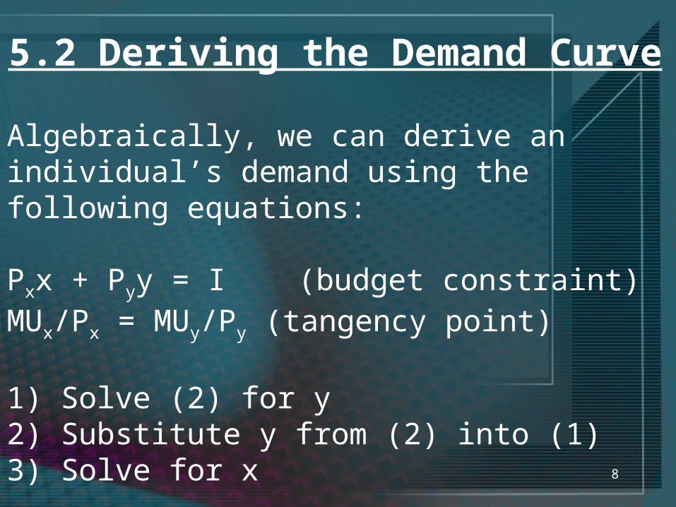
Algebraically, we can derive an individual’s demand using the following equations:
Pxx + Pyy = I (budget constraint)MUx/Px = MUy/Py (tangency point)
1) Solve (2) for y2) Substitute y from (2) into (1)3) Solve for x
5.2 Deriving the Demand Curve

9
General Example:
Suppose that U(x,y) = xy. MUx = y and MUy = x. The prices of x and y are Px and Py, respectively and income = I.
1) x/Py = y/Px
y = xPx/Py
2) Pxx + Py(Px/Py)x = I
Pxx + Pxx = I
3) x= I/2Px

10
Specific Demand Example
Let U=xy, therefore MUx=y and MUy=xLet income=12, Py=1.Graph demand as Px increases from $1 to $2 to $3.
Step 1: Pxx+Pyy=IPxx+y=12
Step 2: MUx/MUy=Px/Py
y/x=Px
y=Pxx

11
Demand Example
Step 1: Pxx+y=12
Step 2: y=Pxx
Step 3: Pxx+Pxx=12x=6/Px
X(1)=6X(2)=3X(3)=2

12
Demand Example
X
PX
2 3 6
Maximizing at each point, we arrive at the following demand curve:
PX = 3PX = 2PX = 1
••
•U increasing

13
Y (units)
X (units)0I = 10
XA=2 XB=10
•10
At a given income, a consumer maximizes using tangency as seen below:
Demand, Choice and Income

14
Y (units)
X (units)0I = 10
I=12
XA=2
XB=3
••
10
When income increases the budget line shifts out, resulting in a new equilibrium
20
Demand, Choice, and Income

15
Y (units)
X (units)0
• • •
10
Income consumption curve
20
The income consumption curve for good x plots all the utility maximization points as income changes. This is shown by shifting the demand curve for x.
5.3 The Income Consumption Curve

16
X (units)
Y (units)
0
10 18 24
PX
X (units)
10 18 24
$2I=92I=68I=40
Income consumption curveU1
U2
U3
I=92
I=68
I=40
The Income Consumption & Demand Curves

17
The income consumption curve for good x also can be written as the quantity consumed of good x for any income level. This is the individual’s Engel Curve for good x.When the income consumption curve is positively sloped, the slope of the Engel curve is positive.

18
• If the income consumption curve shows that the consumer purchases more of good x as her income rises, good x is a normal good.
• Equivalently, if the slope of the Engel curve is positive, the good is a normal good.
• If the income consumption curve shows that the consumer purchases less of good x as her income rises, good x is an inferior good.
• Equivalently, if the slope of the Engel curve is negative, the good is an inferior good.

19
X (units)0
I ($)
92
68
40
10 18 24
Engel Curve
“X is a normal good”

20
• Some goods are normal or inferior over different income levels
Example: Kraft Dinner
a) at extreme low incomes, Kraft dinner consumption goes up as income increases (because starving is bad)
-Kraft Dinner is a normal good at extreme low incomes
b) as income rises, people substitute away from Kraft Dinner to “real foods”
-Kraft dinner is an inferior good at most incomes

21
X (units)
Y (units)
0
13 16 18
I ($)
X (units)
13 16 18
U1U2
U3
I=400
I=300
I=200
200
300
400
Engel Curve
A good can be normal over some ranges and inferior over others
Example: Backward Bending Engel Curve
22
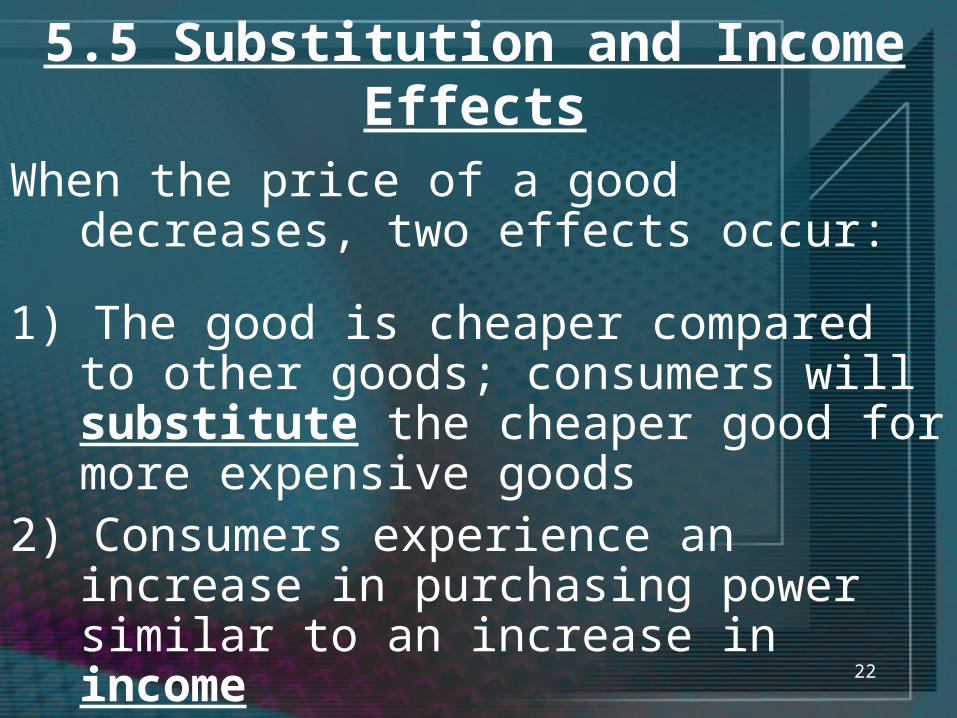
When the price of a good decreases, two effects occur:
1) The good is cheaper compared to other goods; consumers will substitute the cheaper good for more expensive goods
2) Consumers experience an increase in purchasing power similar to an increase in income
5.5 Substitution and Income Effects
23
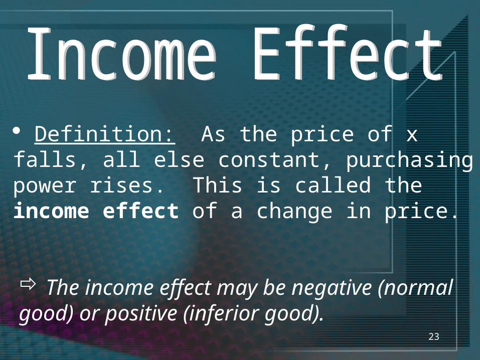
Definition: As the price of x falls, all else constant, purchasing power rises. This is called the income effect of a change in price.
The income effect may be negative (normal good) or positive (inferior good).
24
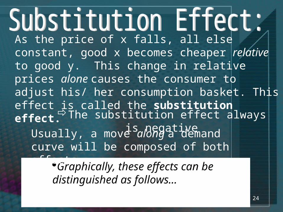
Graphically, these effects can be distinguished as follows…
As the price of x falls, all else constant, good x becomes cheaper relative to good y. This change in relative prices alone causes the consumer to adjust his/ her consumption basket. This effect is called the substitution effect.
The substitution effect always is negativeUsually, a move along a demand
curve will be composed of both effects.

25
0 X (units)
Y (units)
•
•
A
B•C
U1
U2
XA XB XC
BL2
BL1Let Px decrease
Example: Normal Good: Income and Substitution Effects
Substitution
Income
BLd
26
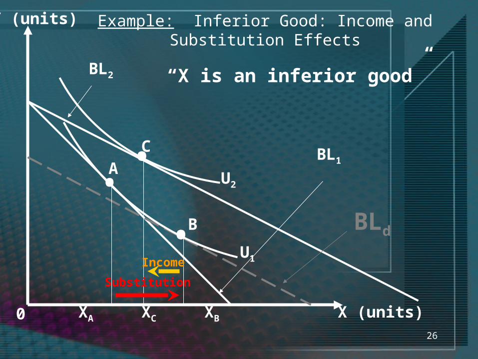
Example: Inferior Good: Income and Substitution Effects
0 X (units)
Y (units)
•
•
A
B
•C
U1
U2
XA XC XB
BL2
BL1
“X is an inferior good”
Substitution
Income
BLd

27
The decomposition budget line (BLd) that satisfies 2 conditions:
1) The budget line represents a change in the price ratio; it must be parallel to the new budget line (BL2)
2) The budget line must be tangent to the old indifference curve (U1)
Finding the DECOMPOSITION Budget Line

28
0 X (units)
Y (units)
•
•
A
B•C
U1
U2
XA XB XC
BL2
BL1
Slope of B1 = -Px1/Py
Slope of B2 = -Px2/Py
Slope of Bd = -Px2/Py
Budget line slopes
Substitution
Income
BLd

29
1) Using initial prices (and tangency), find
a) start point (xa, ya)
b) start utility (Ua)
2) Using final prices (and tancency), find
a) end point (xc, yc)
b) end utility (Uc)
Steps to Finding Substitution and Income Effects:

30
3) Using final prices and start utility for
a) decomposition point (xb, yb)
4) Solve:
a) Substitution Effect: xB-xA
b) Income Effect: xC-xB
Steps to Finding Substitution and Income Effects:
31

32
Solving for x: x = 1/(Px
2)x = 1/(0.5)2
x = 4
Substituting, xA = 4 into the budget constraint:Pxx + Pyy = 100.5(4) + (1)y = 10yA = 8
UA = 2xA1/2
+yA
UA=2(41/2)+8UA=12

33
2) Suppose that px = $0.20. What is the (final) optimal consumption basket?
Using the demand derived in (a), x = 1/(Px
2)xc = 1/(0.2)2
xc = 25
Pxx + Pyy = 100.2(25) + (1)y = 10 yC =5
34
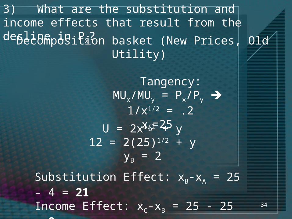
3) What are the substitution and income effects that result from the decline in Px?
Decomposition basket (New Prices, Old Utility)
Tangency: MUx/MUy = Px/Py
1/x1/2 = .2xb=25
U = 2x1/2 + y12 = 2(25)1/2 + y
yB = 2
Substitution Effect: xB-xA = 25 - 4 = 21Income Effect: xC-xB = 25 - 25 = 0

35
If a good is so inferior that the net effect of a price decrease of good x, all else constant, is a decrease in consumption of good x, good x is a Giffen good.
For Giffen goods, demand does not slope down.
When might an income effect be large enough to offset the substitution effect? The good would have to represent a very large proportion of the budget. (Some economists debate the existence of Giffen Goods)
Giffen Goods

36
Example: Giffen Good: Income and Substitution Effects
0 X (units)
Y (units)
•
•
A
B
•C
U1
U2
XB
BL2
BL1
“X is a Giffen good”
Substitution
XC XA
Income

37
The individual’s demand curve can be seen as the individual’s willingness to pay curve.
On the other hand, the individual must only actually pay the market price for (all) the units consumed.
For example, you may be willing to pay $40 for a haircut, but upon arriving at the stylist, discover that the price is only $30
The difference between willingness to pay and the amount you pay is the Consumer Surplus

38
Definition: The net economic benefit to the consumer due to a purchase (i.e. the willingness to pay of the consumer net of the actual expenditure on the good) is called consumer surplus.
The area under an ordinary demand curve and above the market price provides a measure of consumer surplus.
Note that a consumer will receive more surplus from the first good than from the last good.

39
Consumer Surplus
D
Q*
P*EquilibriumOr marketPrice
Quantity
Price
ConsumerSurplus
Consumer Surplus: The difference between what a consumer is willing to pay and what they pay for each item

40
Efficiency of the Equilibrium Quantity
D
10
$8This calculationOnly works forA linear demandcurve
Quantity
Price
ConsumerSurplus
Consumer Surplus = area of triangle=1/2bh=1/2(16-8)(10)=40
$16

41
Consumer Surplus Example 1
Craig’s demand for model cars is given by the demand curve P=20-Q. If model cars cost $10 each, how much consumer surplus does Craig have?
P=20-Q10=20-Q10=Q, Craig buys 10 model cars
Consumer Surplus =1/2bh=1/2(10)(20-10)=50

42
In practice, a consumer’s demand curve is difficult to estimate
Consumer Surplus can be estimated using the optimal choice diagram (budget lines and indifference curves)
Since utility is difficult to measure, consumer surplus is measured through the money needed when a price change occurs:

43
COMPENSATING VARIATION: The minimum amount of money a consumer must be compensated after a price increase to maintain the original utility.
-The consumer’s ORIGINAL Utility is important.
EQUIVALENT VARIATION: The change in money to give a equivalent utility to a price change.
-The consumer’s FINAL Utility is important.

44
Compensating Variation
O X (units)
Y (units)
•
•
A
B
• C
U1
U2
BL2BL1
-A change in the price of x shifts BL1 to BL2
-Consumption moves from point A to point C-A BL at new prices that would maintain original utility is parallel to BL2
M
N
-NM represents the money required to return a consumer to their original utility, consuming at B

45
Equivalent Variation
X (units)
Y (units)
• AC•
U1
U2
BL2BL1
•D
-A change in the price of x shifts BL1 to BL2
-Consumption moves from point A to point C-A BL at old prices that would make the equivalent move to the new utility is parallel to BL1
O
N
Q
-NQ represents the money equivalent to a price change, resulting in consumption at D

46
Compensating and Equivalent Variation
O X (units)
Y (units)
•
•
A B
•C
U1
U2
BL2BL1
•D
-Here a price DECREASE occurs-MN is the max amount a consumer would PAY for this price decrease-NQ is the amount a consumer would be PAID instead of a price decrease
M
N
Q

47
CV and EV Steps1) Calculate ORIGINAL and NEW
consumption points that maximize utility. (Use tangency condition.)
2) Calculate ORIGINAL and NEW utility.3a) Compensating Variation:With ORIGINAL UTILITY and NEW PRICES,
minimize expenditure ECV
CV=I-ECV
3a) Compensating Variation:With FINAL UTILITY and ORIGINAL PRICES, minimize
expenditure EEV
EV=EEV-I

48
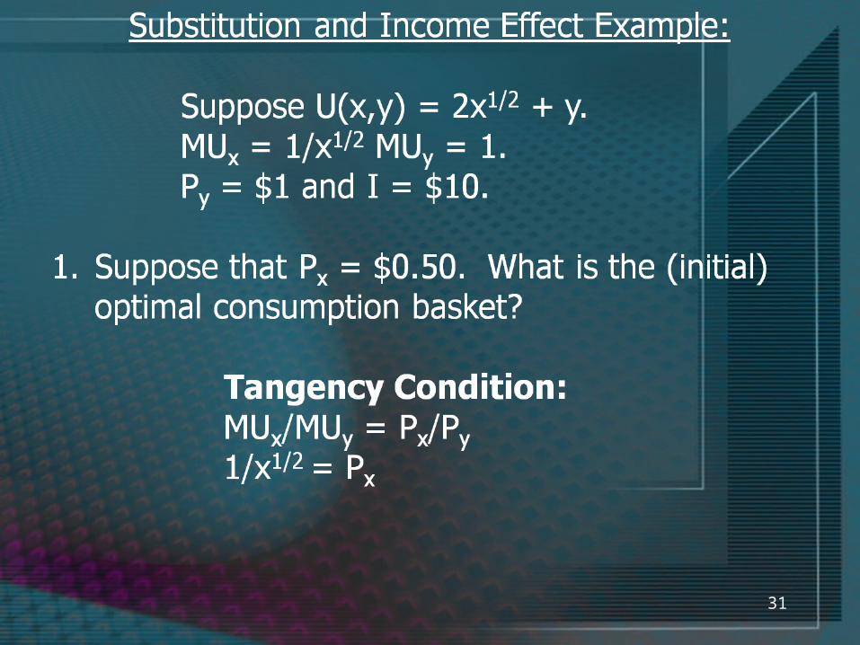
Consumer Surplus Example 2
Hosea’s utility demand for mini xylophones and yogurt (x and y) is represented by U=x2+y2
MUx=2x MUy=2y.
Hosea has $20. Mini xylophones originally cost $2 while yogurt cost $1. Due to an outbreak of mad xylophone disease, price of healthy mini xylophones decreased to $1 each.
Calculate compensating and equivalent variation.

49
Consumer Surplus Example 2
Originally (at point A):MUx/Px=MUy/Py
2x/2=2y/12X=4YX=2Y
PxX+PyY=I2X+Y=205Y=20Y=4
X=2YX=8
After price change (at point C):MUx/Px=MUy/Py
2x/1=2y/1X=Y
PxX+PyY=IX+Y=20X=10
X=Y Y=10
50
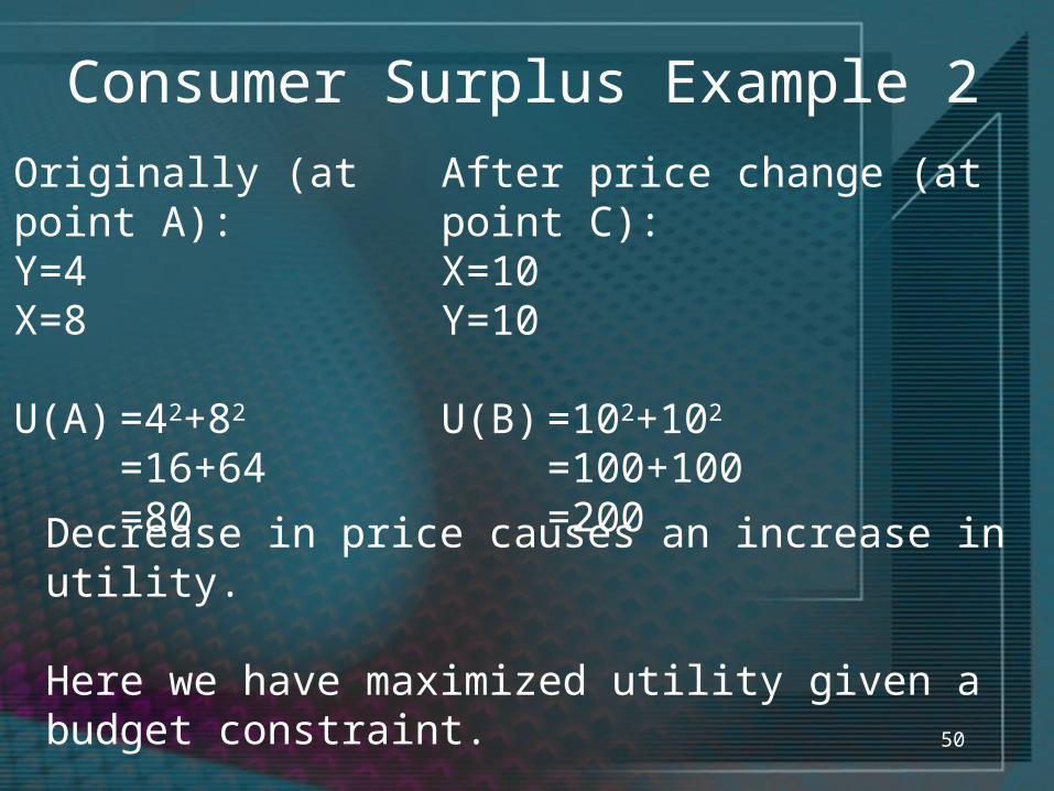
Consumer Surplus Example 2
Originally (at point A):Y=4X=8
U(A) =42+82
=16+64=80
After price change (at point C):X=10Y=10
U(B) =102+102
=100+100=200
Decrease in price causes an increase in utility.
Here we have maximized utility given a budget constraint.

51
Compensating Variation
O X (units)
Y (units)
•
•
A
B
• C
U1
U2
BL2BL1
Compensating variation: at the new prices (budget line parallel to the new budget line), minimize expenditure to achieve the original utility (U1).
M
N

52
Consumer Surplus Example 2Compensating variation: at the new prices (budget line parallel to the new budget line), minimize expenditure to achieve the original utility.
MUx/Px=MUy/Py2x/1=2y/1
X=Y
U=x2+y2
80=x2+x2
40=x2
401/2=x401/2=y

53
Consumer Surplus Example 2Compensating variation: at the new prices (budget line parallel to the new budget line), minimize expenditure to achieve the original utility.
401/2=x401/2=y
PxX+PyY=IX+Y=I
2(401/2)=I12.65=ECV

54
Consumer Surplus Example 2Compensating variation: the maximum amount a consumer will pay to receive a price discount
CV=Original I-ECV
CV=20-12.65CV=7.35
Hosea would pay a maximum of $7.35 to be able to buy mini xylophones at a
reduced price of $1.

55
Equivalent Variation
X (units)
Y (units)
• AB•
U1
U2
BL2BL1
•D
Given the old prices, minimize expenditure to achieve the new utility
O
N
Q

56
Consumer Surplus Example 2Equivalent variation: at the old prices (budget line parallel to the old budget line), minimize expenditure to achieve the new utility.
MUx/Px=MUy/Py2x/2=2y/1
X=2Y
U=x2+y2
200=4y2+y2
40=y2
401/2=y2(401/2)=x

57
Consumer Surplus Example 2Equivalent variation: at the old prices (budget line parallel to the old budget line), minimize expenditure to achieve the new utility.
401/2=y2(401/2)=x
PxX+PyY=I2X+Y=I
2(2(401/2))+401/2=I31.62=EEV

58
Consumer Surplus Example 2Equivalent variation: the minimum amount a consumer would have to be paid to be as well off as a price decrease
EV=EEV-Original IEV=31.62-20
EV=11.62
Hosea would need to be paid $11.62 to be as well off as a decrease in the price of
xylophones.

59
Note that in the previous example CV did not equal EV ($7.35 is not equal to $11.62).This occurs because the price change has a non-zero income effect.Although CV and EV try to approximate Consumer surplus, generally neither will
However,If the income effect is zero, CV=CS=EV
-ie: Quasi-Linear Utility functions.

60
COMPENSATING VARIATION:
Original Utility and new prices
EQUIVALENT VARIATION:
Final Utility and old prices

61
In the economy, each market has many individuals demanding a goodEach individual maximizes their own utility when deciding on the amount they will buyEach individual has a maximum price they will pay and a maximum amount of the item they would want
Ie: I’d pay $5 per episode of House, up to 20 episodes…how much would you pay?
The sum of individual demand creates market demand

62
Consider the following individuals’ demand for Sushi:
Price $1 $2 $3 $4
Craig’s Demand
8 6 4 2
Kristy’s Demand
6 3 0 0
Total Demand
14 9 4 2

63
Market Demand
OSushi
Price
•
• DM•DC
DK
Here the individual demand curves (DK and DC) combine to form market demand (DM).
$4
2
$2
3 6 9
•

64
Algebraically the demand curves are as follows:
5 P when 0
5 P 3 when 2P-10
3P when 519
{)(
:us give tocombine These
3 P when 0
3 P when 39{)(
5 P when 0
5 P when 210{)(
P
PQ
PPQ
PPQ
m
k
C

65
Market Demand
OSushi
Price
•
• DM•DCDK
In section A of market demand, Qm=Qc+QK. (it is important to add the normal form: Q=f(P), not the inverse form: P=f(Q).)In section B of market demand, Qm=QC.
$4
2
$2
3 6 9
•
66
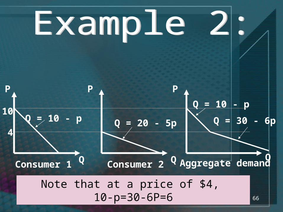
Q = 10 - p
Consumer 1
Q = 20 - 5p
Consumer 2 Aggregate demand
4
10
Q Q Q
P P P
Q = 10 - p
Q = 30 - 6p
Note that at a price of $4, 10-p=30-6P=6

67
Generally we assume that one consumer’s demand does not depend on the demand of others
In some cases, a person’s demand has an EXTERNAL effect on another’s demand – an externality exists
You are less likely to purchase a guard dog if your neighbour has oneYou are more likely to eat sushi if all your friends do

68
If one consumer's demand for a good changes with the number of other consumers who buy
the good, there are externalities.If one person's demand with the
number of other consumers, then the externality is positive.
If one person's demand with the number of other consumers, then the externality is
negative.
Examples: Telephone (physical network) Software (virtual network)
decreases
increases

69
•Apple’s IPad has been growing in popularity and is an example of a bandwagon effect.
•People often buy an iPad because their friends have it
-They are purchased to “BE COOL”-They are purchased because more people
are using iTunes for games and aps than other alternatives
If iPad prices decrease, an individual’s demand will increase due to the new price and due to the number of friends who buy iPads due to the new price

70
Example: IPads and The Bandwagon Effect
X (units)
PX
DOriginal
DNew
Market Demand
•• •
A
B C
20
10
30 38 60
PurePriceEffect
Bandwagon Effect
Bandwagon Effect (increasedquantity demanded when moreconsumers purchase)

71
•When the first few Hybrid Cars came to Edmonton, everyone wanted them
•Even though studies showed they (originally) cost more over their lifetime than a normal car and may actually pollute the environment more, people wanted them as a status symbol
•As prices decreased and more cars become available, demand became more realistic
•This is an example of the SNOB EFFECT: demand decreases as others buy the good

72
Example: The Snob Effect
X (units)
PX
Market Demand
••
A
C
1200
900
Snob Effect (decreasedquantity demanded when moreconsumers purchase)
D10 Cars
D50 Cars
•B
Pure Price Effect
Snob Effect
10 13 18

73
Externalities Example 1
The newest craze to hit the market is cell phone implants – not only do you never lose your phone, but you can now talk to all your friends IN YOUR MIND!
The one catch is that IMPhones can only call other IMPhones. Estimated demand for IMPhones is Q=5,000-10P and current prices are $100 each. After prices drop to $80, demand is seen to be 4500 units. Calculate and explain the externality.

74
Externalities Example 1Original Demand: Q=5,000-10P
Q=5,000-10(100)Q=4,000
New Demand along original curve:Q=5,000-10PQ=5,000=10(80)Q=4,200
Externality = Actual Demand-Estimated Demand
= 4,500-4,200= 300

75
Externalities Example 1
There is a POSITIVE EXTERNALITY or bandwagon effect of 300 units; the demand curve shifts due to others
buying the new IMPhone.
(IMPhones become more valuable as more people install them.)

76
Basic economic theory states that as an individual’s wage increases they will work more; the benefit from an additional hour of work outweighs the benefit from an additional hour of watching TV (House of course)
In practice however, high wage earners tend to work less than minimum wage earners
Is this the end of economics as we know it?

77
Assume:
“Labor” includes all work hours when the consumer is earning income. (L hours per day at wage rate w per hour. Let w = $5)
“Leisure” includes all nonwork activities (so hours of leisure, l = 24 – L)
U= U(y,l)
Utility depends on consumption of a composite good (y) and hours of leisure.
78
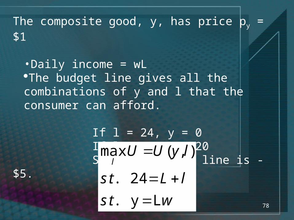
The composite good, y, has price py = $1
•Daily income = wLThe budget line gives all the combinations of y and l that the consumer can afford.
If l = 24, y = 0 If l = 0, y = 120 Slope of budget line is -$5.
wts
lLts
lyUUl
Ly ..
24 ..
),(max

79
Labour and Leisure
OLeisure (l)
Y (units)
•
w=5
As wage is increasing, a consumer’s maximization may cause him/her to increase or decrease leisure:
120
w=10
w=15
w=20
w=25
240
360
600
480
••• •

80
If leisure is a normal good, the income effect on leisure is positive
Therefore, the income effect on labor is negative (labor is a “bad”)
The substitution effect leads to less leisure and more labor as w increases.
As w increases, the consumer feels as though he has more income because less work is needed to buy a unit of y. This creates an income effect.

81
This information can be used to construct the consumer’s labor supply function, L(w).If the substitution effect of a
wage increase outweighs the income effect, the labor supply slopes upwards
If the income effect of a wage increase outweighs the substitution effect, the labor supply curve bends backwards.

82
Example: A Backward Bending Supply of Labor
Leisure (hours)24
Daily Income in units of composite good, Y
W=15
W=25
•
••
U3
U5
600
480
360
240
120
12 13 14 15
•
Substitution Effect (LB-LA) Income Effect (LC-LB)
C
AB
Wage increases from $15 to $25, causing an increase in leisure time
Substitution
Income

83
The Consumer Price Index (CPI) is an important measure of inflation and prices
CPI is an aggregate measure of the cost on an average “basket” of goods each year
CPI is used for price increases and wage increases from year to yearThe Canadian Government used the CPI for taxes and payments
Calculation of the CPI can lead to a substitution bias:

84Food
Clothing
0 80
40
30 •
•A
B
Given initial prices of Pf=$3 and Pc=$8, an average consumer will consume 80 food and 30 clothing for a total cost of $480.
CPI
60
At new prices of Pf=$6 and Pc=$9, an average consumer will consume 60 food and 40 clothing for a total cost of $720.

85
The “Ideal” CPI would be the ratio of the new expenses to the old expenses: $720/$480=1.5
In reality, it is difficult and costly to track consumption as so many goods are consumed: toilet paper may change by -2% one year while cheese increases by 5%
For practical reasons, a set consumer basket is used from year to year; only prices chance
This causes a “substitution bias”: most consumers will substitute away from expensive goods, yet the CPI assumed no substitution occurs

86Food
Clothing
0 80
40
30 •
•
A
B
Practically, the CPI assumes every year consumption occurs at A. In year 2, a consumer assumed to purchase A at a cost of $750 would much rather purchase basket C.
CPI
60
• C

87
The “Practical” CPI would be the ratio of the new estimated cost of living to the old cost of living: $750/$480=1.5625
In reality, the cost of living increased by 50%, yet the CPI estimated an increase in the cost of living of 56.25%.
Every year the CPI shows growth of less than 10%.
Economists estimate this growth may be 0.5%-1.5% too high, which in the US accounts for billions of dollars of increased spending each year

88
Chapter 5 Key ConceptsDeriving Demand
Price Consumption CurveDemand CurveIncome Consumption CurveEngel Curve
Substitution and Income EffectsDecomposition Budget Line
Consumer Surplus

89
Chapter 5 Key ConceptsCompensating & Equivalent VariationMarket Demand
ExternalitiesLabor and Leisure
Backwards Bending Labor SupplyConsumer Price Index (CPI)