Embed Size (px)
Citation preview

1
Education 1 - Funding
© Allen C. Goodman, 2008

2
Some Numbers
• Government puts together lots of numbers.
• Good source – Digest of Education Statistics, http://nces.ed.gov/search/

3
Share has risen but not that much
Percentage of GDP on Education
0
1
2
3
4
5
6
7
8
1940 1950 1960 1970 1980 1990 2000 2010
Year
Pe
rce
nta
ge
s
All
Elem,Sec
Colleges

4
State/DC Total
New York.......................................................................14,884New J ersey.....................................................................14,630District of Columbia..........................................................13,446Vermont..........................................................................12,614Connecticut....................................................................12,323Massachusetts................................................................11,981Rhode Island...................................................................11,769Delaware........................................................................11,633Alaska...........................................................................11,460Wyoming.........................................................................11,197Pennsylvania..................................................................11,028Maryland........................................................................10,670Maine.............................................................................10,586New Hampshire...............................................................10,079Wisconsin.......................................................................9,970Hawaii...........................................................................9,876Ohio...............................................................................9,598
Michigan........................................................................9,572
Virginia...........................................................................9,447West Virginia...................................................................9,352Illinois............................................................................9,149United States................................................................9,138Minnesota......................................................................9,138Indiana...........................................................................8,793Nebraska.......................................................................8,736North Dakota...................................................................8,603
Montana........................................................................8,581Georgia..........................................................................8,565Oregon...........................................................................8,545California........................................................................8,486Louisiana........................................................................8,402Kansas..........................................................................8,392Iowa..............................................................................8,360Missouri........................................................................8,107South Carolina.................................................................8,091New Mexico...................................................................8,086Colorado.........................................................................8,057Arkansas........................................................................7,927Washington.....................................................................7,830Florida............................................................................7,759Kentucky........................................................................7,662South Dakota..................................................................7,651Alabama........................................................................7,646Texas.............................................................................7,561North Carolina.................................................................7,388Nevada...........................................................................7,345Mississippi.....................................................................7,221Oklahoma.......................................................................6,961Tennessee.......................................................................6,883Arizona...........................................................................6,472Idaho..............................................................................6,440Utah................................................................................5,437
Per Pupil Elem-Sec
2005-2006
http://ftp2.census.gov/govs/school/elsec06_sttables.xls

5
Per pupil expenditures, 2006-2007
Salaries and Employee All
Total 1 wages benefits Compensation
United States................................................................9,666 5,923 1,973 7,895
Illinois............................................................................9,555 5,916 1,689 7,605Indiana...........................................................................8,938 5,094 2,534 7,628Iowa..............................................................................8,769 5,661 1,724 7,384Michigan........................................................................9,912 5,503 2,617 8,120Minnesota......................................................................9,539 6,142 1,804 7,947Ohio...............................................................................9,799 6,067 2,140 8,207Wisconsin.......................................................................10,267 5,542 2,891 8,433
Geographic area
Source: Excel spreadsheet

6
General Issue
• Equality of Funding• We looked at this a little bit earlier on.• Suppose you have 2 districts
– District1 – Tax Base = $200,000– District2 – Tax Base = $100,000
• If they both have a 2.5% property tax rate, then D1 will raise $5,000 for schools, while D2 will raise only $2,500 for schools.
• For D2 to raise as much they must pay double the tax “price.”

7
Opportunity
• Most of our Tiebout discussion has to do with localities picking their tax rates and their levels of public services.
• It suggests however that poorer people will get lower levels of public services.
• Many view this type of thing as “unfair.”• Premise here is that unequal inputs
unequal outputs. We’ll talk more about outputs in next class.

8
Various Ways to Equalize Aid
• Try to equalize expenditures
• Try to equalize the tax base– Fisher argues that the tax base equalization
could induce districts to spend more, by decreasing the cost per $ spent.

9
GTB Formula (and worksheet)
Consider a formula of the type:
Gi = B + (V* - Vi) Ri, where:
Gi = grant
B = Basic or Foundation Grant
V* = Guaranteed per-public tax base
Vi = Per pupil tax base in district i.
Ri = Tax rate per thousand dollars in district i.
Difference tomake up Tax effort!

10
GTB Formula (and worksheet)Consider a formula of the type:
Gi = B + (V* - Vi) Ri, where:
Gi = 0 + ($200,000 – $50,000) ($40/$1,000), where:
Gi = grantB = Basic or Foundation GrantV* = Guaranteed per-pupil tax baseVi = Per pupil tax base in district i.Ri = Tax rate per thousand dollars in district i.
Gi = $6000; own effort = $2000
If you raise R by $1 in your district, it is raised by (V* - V)/V times; Here (200 – 50)/50. So a $1 tax gets a $3 match.Implicit tax price = 1/(1+3) or 25%. Let’s look at spreadsheet.
11
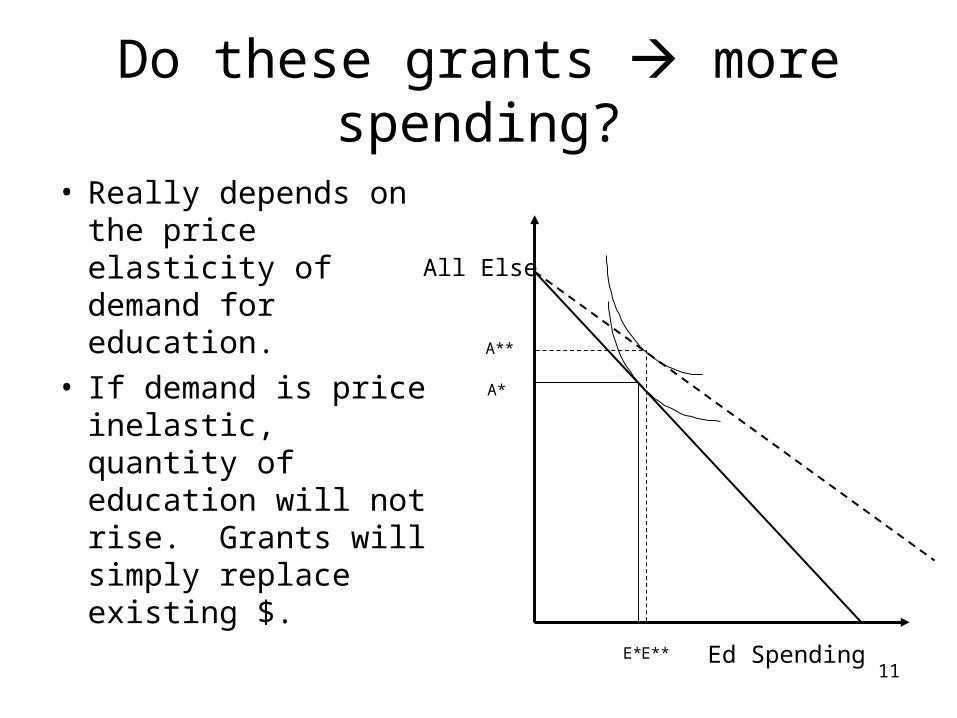
Do these grants more spending?
• Really depends on the price elasticity of demand for education.
• If demand is price inelastic, quantity of education will not rise. Grants will simply replace existing $.
Ed Spending
All Else
E*
A*
A**
E**

12
Hoxby (2001)
• Looks at states in 1990.• Relates characteristics of state’s financing
systems to actual spending.• Spending increased with GTB formulas
and lower tax prices for low-wealth, low-spending districts, but …
• Substantial amount of equalization comes by limiting the highest spending districts called “leveling down.”

13
Coefficient of variation
• The coefficient of variation is a dimensionless number that allows comparison of the variation of populations that have significantly different mean values.
• It is often reported as a percentage (%) by multiplying the above calculation by 100.
• Idea: If you’re comparing high income districts to low income districts, you might expect the high income districts to vary a little more because there’s more of a “top end.”
• CV controls for the higher mean.
.std deviationCV
mean

14
Examples – D1, D2, D3 are distributions of School Districts
Coefficient of Variation
D1 D2 = D1 + 500 D3 = 1.1*D1
5000 5500 5500
6600 7100 7260
7000 7500 7700
8000 8500 8800
9000 9500 9900
10000 10500 11000
11000 11500 12100
12000 12500 13200
Std. Dev. 2370 2370 2607
Mean 8575 9075 9432.5
CV 0.27637324 0.26114607 0.27637324

15
Michigan School Finance
• Prior to 1974, CV was about 0.16.
• By 1980, it was 0.17, and by 1994 it had increased to 0.23.
• In 1978 local property taxes about ½ of school revenue.
• By 1994 local property taxes about 2/3 of revenue.
• Property tax burden was 7th highest in US.
16
In 1994 – new system
• Foundation guarantee, F– F is determined by 1993/4 level, plus allowed
annual increases.– Districts > $5000 get % increases equal to %
growth of state school aid revenue multiplied by basic foundation (which started at 5000).
– Those below $5000 receive up to double these percentage amounts.

17
18 Mills = 1.8%
• Each district is supposed to levy 1.8%.
• State provides the rest.
• Highest spending districts levy additional property taxes to reach the levels they want.
• Over time foundation grows, and would presumably lower CV.
State largely substituted itself for thelocal property tax base. If state $/studentwere larger than locality, local tax bite fell.
18
Cullen and Loeb (2004)
1. State now generates more than 75% of funding for schools.
2. Most of the funding comes from increase in state sales tax from 4% to 6%
3. Level of school spending increased by 9% (real) from 1990 to 1998.
4. CV fell from 0.22 in 1991 to 0.13 in 2000.
Cullen, Julie Berry and Susanna Loeb, 2004. “School finance reform in Michigan: evaluatingProposal A” in J. Yinger, ed., Helping Children Left Behind: State Aid and the Pursuit ofEducational Equity (Cambridge, MA: MIT Press), pp. 215-50.

19
Issues
• Although inputs , did outputs ?
• Some high spending districts were not allowed to spend as much as they would like.– Solution? Fees like athletic or music fees.– Stop providing items where there are
plausible private substitutes – e.g. driver training.

20
More Issues
• Per pupil funding, while plausible, can impose hardships on districts with falling enrollments.
• Consider SD with:– 4 elem schools (50 students/grade * 5 grades
each) = 1000 students– 1 middle school (200 students/grade * 3
grades)– 1 HS (800 students over 4 grades)
2400 Students
21
More Issues
• Consider SD with:– 4 elem schools (50 students * 5 grades each) = 1000
students– 1 middle school (200 students * 3 grades)– 1 HS (800 students)
• Suppose enrollment in ES falls by 4 students/grade = 8%, or 2 students/class.
• Fall of 80 students. ES Funds fall by 8%. Total students by 3%.
• What do you cut?

22
Suggests
• Short term problems in all areas where schools are growing.
• Places like southern Oakland County.– Ferndale, Royal Oak, Hazel Park are losing students.– Walled Lake, South Lyon are gaining students. You
have about the same numbers of students, but you have schools in the wrong places.
• Political problems consolidating and/or closing schools.
• Look at City of Detroit!• Is this formula necessarily bad? Is there
something better?