Embed Size (px)
Citation preview

1
Property Tax
© Allen C. Goodman, 2015

Great Lakes.................................................................................
36.9 36.8 33.6 36.0 32.8 33.8 34.8 35.1 34.6 34.5 34.6 36.6 37.5 35.6 34.4
Illinois.................................................................................
36.7 35.7 34.2 38.6 38.1 38.1 39.5 37.6 37.6 37.5 38.5 41.9 42.8 40.8 38.4
Indiana.................................................................................
36.8 35.6 32.0 30.7 34.6 35.2 32.5 37.7 33.7 28.5 29.4 30.4 32.8 27.5 26.5
Michigan.................................................................................
37.5 42.5 38.2 42.7 29.0 32.0 35.8 36.6 37.6 39.2 37.6 40.2 40.2 37.5 36.7
Ohio.................................................................................
37.7 33.6 28.2 29.7 28.8 29.4 28.7 28.7 28.6 29.2 29.1 29.6 30.0 29.4 29.0
Wisconsin.................................................................................
34.5 35.0 34.6 34.9 33.4 34.7 36.3 36.4 36.0 36.0 36.5 38.4 39.8 38.9 37.9 2
http://www.taxpolicycenter.org/taxfacts/displayafact.cfm?Docid=517
Region and State 1977 1982 1987 1992 1997 2002 2004 2005 2006 2007 2008 2009 2010 2011 2012
United States .................................................................................
35.5% 30.8% 29.9% 32.2% 30.1% 30.8% 31.5% 30.6% 30.2% 30.3% 30.8% 33.7% 34.7% 33.2% 32.1%

3
Rule
Tax Variable
Agent
Actual or True Mkt Value
How do you assess? Schematic from Figure 13.1

4
How do you assess? Schematic from Figure 13.1
Rule
Tax Variable
Agent
Actual or True Mkt Value
Assessed orTaxable Value
Ratio ruleExempt Property
Assessor
5
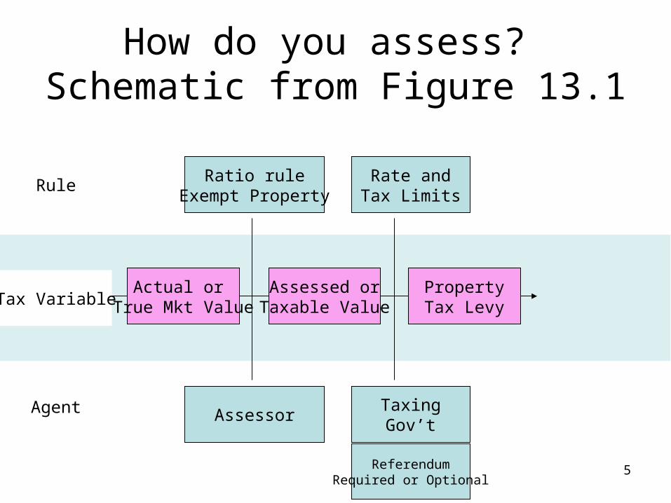
Rule
Tax Variable
Agent
Actual or True Mkt Value
Assessed orTaxable Value
PropertyTax Levy
Ratio ruleExempt Property
Assessor
Rate andTax Limits
TaxingGov’t
ReferendumRequired or Optional
How do you assess? Schematic from Figure 13.1

6
Rule
Tax Variable
Agent
Actual or True Mkt Value
Assessed orTaxable Value
PropertyTax Levy
PropertyTax Revenue
Ratio ruleExempt Property
Assessor
Rate andTax Limits
TaxingGov’t
ReferendumRequired or Optional
Tax Collector
How do you assess? Schematic from Figure 13.1

7
How Property is Assessed
• Comparative Sales – What has been the value of other recently sold properties?
• Cost Approach – How much did the property cost to build?– How much have construction costs changed?– How much has it depreciated?
• Income Approach– What is net present value of income to be
generated by property?
Most oftenfor residences.
Cost and income approachesare most often used for
commercial property.

8
Comparables
• If you’re buying (appraising) a house, you do this.
• Look at house you’re buying (appraising)– Find other comparable houses.– See how they differ.– Adjust values based on differences.
• (Sometimes) float baseline values up according to neighborhood specific inflation factors.

9
Adjustments to make “comparable”
similar to appraised house

10
On-Line Tools
• There are also on-line appraisal tools
• Here’s one.– http://www.zillow.com

11
Proposal A in MichiganProposal A Spreadsheet
Tax RateRate 1.5%
Value % CPI Taxable Effective Taxes on MobilityYear Value Increase Inflation Value Taxes Rate Value Tax
1994 200,000 200,000 3,000 1.50% 3,000 01995 220,000 10.0% 2.5% 205,017 3,075 1.40% 3,300 2251996 240,000 9.1% 2.8% 210,808 3,162 1.32% 3,600 4381997 255,000 6.3% 2.9% 216,992 3,255 1.28% 3,825 5701998 265,000 3.9% 2.2% 221,766 3,326 1.26% 3,975 6491999 275,000 3.8% 1.3% 224,704 3,371 1.23% 4,125 7542000 290,000 5.5% 2.2% 229,723 3,446 1.19% 4,350 9042001 300,000 3.4% 3.5% 237,686 3,565 1.19% 4,500 9352002 320,000 6.7% 2.7% 244,183 3,663 1.14% 4,800 1,1372003 360,000 12.5% 1.4% 247,581 3,714 1.03% 5,400 1,6862004 400,000 11.1% 2.2% 253,131 3,797 0.95% 6,000 2,2032005 420,000 5.0% 2.6% 259,713 3,896 0.93% 6,300 2,4042006 420,000 0.0% 3.5% 268,868 4,033 0.96% 6,300 2,2672007 400,000 -4.8% 3.2% 277,516 4,163 1.04% 6,000 1,8372008 375,000 -6.3% 2.9% 285,472 4,282 1.14% 5,625 1,343
12
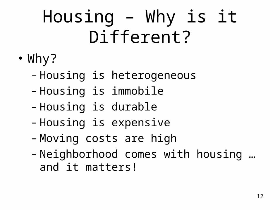
Housing – Why is it Different?
• Why?– Housing is heterogeneous– Housing is immobile– Housing is durable– Housing is expensive– Moving costs are high– Neighborhood comes with housing … and it
matters!

13
Heterogeneous?
• Dwellings differ in:– house size (sq. feet)– lot size (sq. feet)– configuration– quality
• People seem to value these qualities differently.

14
Immobile?
• It is where it is. Where you buy it, you get:– Accessibility (to good and bad things)– Package of local public services– Environmental quality
• Further– You can’t (really) “move” houses– You can’t rebundle them (use half of two
different houses at the same time).
15
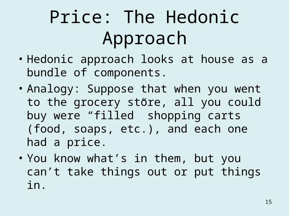
Price: The Hedonic Approach
• Hedonic approach looks at house as a bundle of components.
• Analogy: Suppose that when you went to the grocery store, all you could buy were “filled” shopping carts (food, soaps, etc.), and each one had a price.
• You know what’s in them, but you can’t take things out or put things in.

16
Price: The Hedonic Approach
• How do you figure out what the individual components are worth?
• A> If you had a large sample of carts, and each had different amounts of goods in them, then you could come up with the value of the individual components.

17
Example for Hedonic Prices
• Suppose that sq. feet of living space was ALL that mattered in the price of house.
• You collect data on lots of houses.
Sq. feet
Pric
e

18
Example for Hedonic Prices
• What does this suggest?– A> Bigger
houses have more value.
• Let’s draw a line.
Sq. feet
Pric
e
??

19
Example for Hedonic Prices
• Line has a form:
Price = a + b*size
Sq. feet
Pric
e
• What does a mean?
• What does b mean?
a
slope = b

20
Example for Hedonic Prices
• Says that for each additional sq. ft., house price is $b more.
Sq. feet
Pric
e
• Although it is hard to think of, we could draw this diagram in n dimensions!
a
slope = b
b is the hedonic price of house size.

21
n dimensions?
Let’s look at a house with 2000 sq.ft., 5 rooms for $75,000 P
rice
Sq. feet20005
75
Let’s look at a house with 3000 sq.ft., 6 rooms for $100,000
3000
6
100
Rooms
Line has a form: Price = a + b*size + c*rooms

22
How do you do this?
• This allows us to impute the valuations of all kinds of components of the bundle. The incremental valuation is called the “hedonic price.” Was invented in Detroit!
• Here’s a database with examples from Detroit for 1989.
• American Housing Survey.

23
Metro Detroit Hedonic Regressions - 1989
Dep: House Value
Linear Linear Semi-Log
Coeff Std. Err. Coeff Std. Err. Coeff Std. Err.Intercept -2,871 4,829 -2,305 5,508 10.1185 0.0741ROOMS 10,359 743 9,720 709 0.1133 0.0095BUILT -971 57 -710 59 -0.0085 0.0008BATHRMS 24,295 2,174 23,319 2,075 0.2090 0.0279GARAGE 18,650 2,609 18,401 2,491 0.3771 0.0335WAYNE -876 3,419 -0.0122 0.0460DETROIT -31,863 3,039 -0.7147 0.0409OAKLAND 8,010 3,366 0.0331 0.0453MACOMB -3,309 3,611 0.0062 0.0486
R2 0.44118 0.49886 0.51149
24
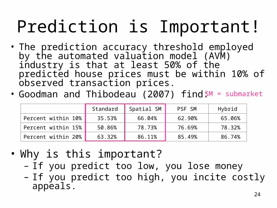
Prediction is Important!• The prediction accuracy threshold employed by the
automated valuation model (AVM) industry is that at least 50% of the predicted house prices must be within 10% of observed transaction prices.
• Goodman and Thibodeau (2007) find:
Standard Spatial SM PSF SM Hybrid
Percent within 10% 35.53% 66.04% 62.90% 65.06%
Percent within 15% 50.86% 78.73% 76.69% 78.32%
Percent within 20% 63.32% 86.11% 85.49% 86.74%
• Why is this important?– If you predict too low, you lose money– If you predict too high, you incite costly appeals.
SM = submarket