Embed Size (px)
Citation preview

1. Element of Investment Cost
Consider a situation in which the equipment and
related support for a new Computer-Aided Design/
Computer-Aided Manufacturing (CAD/CAM)
workstation are being acquired for your engineering
department. The applicable cost elements and
estimated expenditures are as follows:
Cost Element Cost
Lease a telephone line for communication RM 1,100/month
Lease CAD/CAM software (includes installation and debugging)
RM 550/month
Purchase hardware (CA/CAM workstation)
RM 20,000
Purchase high-speed modem
RM 250
Purchase a high-speed printer
RM 1,500
Purchase a four-color plotter
RM 10,000
Shipping costs
RM 500
Initial training (in house) to gain proficiency with CAD/CAM software
RM 6,000
What is the investment cost of this CAD/CAM System?
Solution:
The investment cost in this is the sum of all the cost elements
except the two monthly lease expenditures-specifically, the sum
of the initial costs for the CAD/CAM workstation, modem, printer,
and plotter (RM 31,750); shipping cost (RM500); and the initial
training cost (RM 6,000). These cost elements result in a total
investment cost of RM 38,250. The two cost elements that involve
lease payments on a monthly basis (telephone line and
CAD/CAM software) are part of the recurring cots in the operation
phase.

2. Choosing the most Economic Material for Part
A good example of this situation is illustrated by the part
below which annual demand is 100,000 units. The part shown
is produced on a high-speed turret lathe, using 112 screw-
machine steel costing RM 0.30 per kg. A study was
conducted to determine whether it might be cheaper to use
brass screw stock, costing RM 1.40 per kg. Because the
weight of steel required per piece was 0.0353kg and that
brass was 0.0384 kg, the material cost per piece was RM
0.016 for steel and RM 0.0538 for brass. However, when the
manufacturing engineering department was consulted, it was
found that, although 57.1 defects parts per hour were being
produced by using steel, the output would be 102.9 defect-
free part per hour if brass were used.
Which material should be used for this part?
Figure1: Small Screw Machine Product
¼
¼¾
1
Solution:
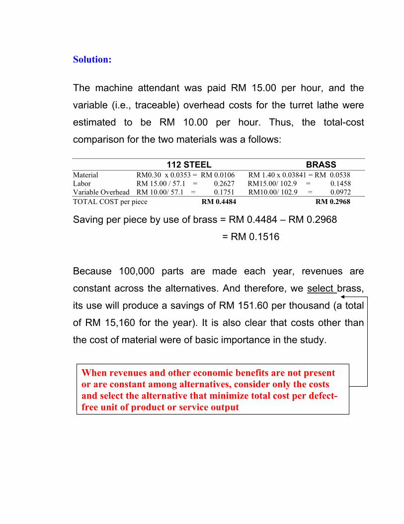
The machine attendant was paid RM 15.00 per hour, and the
variable (i.e., traceable) overhead costs for the turret lathe were
estimated to be RM 10.00 per hour. Thus, the total-cost
comparison for the two materials was a follows:
112 STEEL BRASS Material RM0.30 x 0.0353 = RM 0.0106 RM 1.40 x 0.03841 = RM 0.0538
Labor RM 15.00 / 57.1 = 0.2627 RM15.00/ 102.9 = 0.1458
Variable Overhead RM 10.00/ 57.1 = 0.1751 RM10.00/ 102.9 = 0.0972
TOTAL COST per piece RM 0.4484 RM 0.2968
Saving per piece by use of brass = RM 0.4484 – RM 0.2968
= RM 0.1516
Because 100,000 parts are made each year, revenues are
constant across the alternatives. And therefore, we select brass,
its use will produce a savings of RM 151.60 per thousand (a total
of RM 15,160 for the year). It is also clear that costs other than
the cost of material were of basic importance in the study.
When revenues and other economic benefits are not present
or are constant among alternatives, consider only the costs
and select the alternative that minimize total cost per defect-
free unit of product or service output

3. Personal Interest Problem
Don Ngoc prides himself on how much money he can save
by being frugal. Today Don Ngoc need 15 gallons of gasoline
to top off his automobile’s gas tank. If he drives eight
kilometer (round trip) to a gas station on the outskirts of
town, Don Ngoc can save RM 0.10 per gallon on the price of
gasoline. Suppose gasoline costs RM 2.00 per gallon and
Don’s car gets 25 km per gallon for in-town driving.
Should Don Ngoc make the trip to get less expensive
gasoline? What other factors (cost and otherwise) should
Don Ngoc consider in his decision making?
Solution:
Savings = 15 gallons x RM 0.10/gallon = RM 1.50 for the trip.
Savings per kilometer driven = RM 1.50/ 8km = RM 0.1875 per
km.
If Don Ngoc can drive his car for less than RM 0.1875 per km,
he should make the trip.
The cost of gasoline only for the trip is
(8km ÷ 25 km per gallon) (RM 2.00 per gallon) = RM 0.64,
but other costs of driving, such as insurance, maintenance, and depreciation,
may also influence Don’s decision. Hat is the cost of an accident, should Don
have one during his trip to purchase less expensive gasoline? If Don makes
the trip weekly for a year, should this influence his decision?
4. Student tuition Suppose student tuition at Melaka University is RM 100 per
semester credit hour. The state supplements school revenue
by matching student tuition ringgit for ringgit. Average class
size for a typical three-credit course is 50 students. Labor
costs are RM 4,000 per class, materials costs are RM 20 per
student per class, and overhead costs are RM 25,000 per
class.
a. What is the multifactor productivity ratio for this course
process?
b. If instructor work an average 14 hours per week for 16
weeks for each three-credit class of 50 students, what is
the labor productivity ration?

Solution:
a. Multifactor productivity is the ratio of the value of output to the value of input resources.
Value of output = 50 students 3 credit hours RM100 (T) + RM 100 (SS)
Class student credit hours
= RM 30,000
Value of input = Labor + Materials + Overheads
= RM 4,000 + (RM20/student X 50students/Class) + RM 25,000
= RM 30,000/ class
Multifactor productivity = Output = RM 30,000 /class = 1 Input RM 30,000/ class
b. Labor productivity is the ratio of the value of output to labor hours. The value of output is the same as in part (a), or RM 30,000/class, so…
Labor hours input = 14 hours 16weeks = 224 hours/class Week class
Labor productivity = Output = RM 30,000 /class Input 224 hours/ class
= RM 133.93
T = Tutorial Cost SS = State Supplement

5. Productivity Natalie Attire makes fashionable garments. During a
particular week employees worked 360 hours to produce a
batch of 132 garments, of which 52 were ‘seconds’ (meaning
that they were flawed). Seconds are sold for RM 90 each at
Attire’s Factory Outlet Store. The remaining 80 garments are
sold to retail distribution, at RM 200 each. What is the labor
productivity ratio of this manufacturing process?
Solution:
Value of output = (52defectivexRM90/defective)+(80garmentsxRM200/ garments)
= RM 20,680
Labor hours of input = 360 hours
Labor productivity = Output = RM 20,680 Input 360 hours
= RM 57,44 in sales per hour.

Defining the Problem and Developing Alternatives
1. Manufacturing Company
The measurement team of a small furniture-manufacturing
company is under pressure to increase profitability in order
to get a much-needed loan from the bank to purchase a
modern pattern-cutting machine. One proposed solutions is
to sell waste wood chips and shavings to a local charcoal
manufacturer instead of using them to fuel space heaters for
the company’s office and factory areas.
a. Define the company’s problem. Next, reformulate the
problem in a variety of creative ways.
b. Develop at least one potential alternative for your
reformulated problems in part (a).
Solution: a. The company’s problem appears to be that revenues are not
sufficiently covering costs. Several reformulations can be posed:
1. The problem is to increase ( ) revenues while reducing ( ) costs
2. The problem is to maintain revenues while reducing ( ) costs
3. The problem is an accounting system that provides distorted cost information
4. The problem is that the new machine is really not needed (and hence here is no need for a bank loan)

b. Based on reformulation 1, an alternative is to sell woods chips and shavings as long as increased revenues ( ) exceed extra expenses that may be required to heat the buildings.
Another alternative is to discontinue the manufacture of specialty items and concentrate on standardized, high volume products. Yet another alternative is to pool purchasing, accounting, engineering, and other white-collar support services with other mall firms n the area by contracting with a local company involved in providing these services.

2. Rent Building
A friend of yours bought a house building in Taman Tasik
Utama for RM 100,000 in nearby Melaka University campus.
She spent RM 10,000 of her own money for the building and
obtained a mortgage from a local bank for the remaining RM
90,000. The annual mortgage payment to the bank is RM
10,500. Your friend also expects that annual maintenance on
the house will be RM 15,000. There are four rooms (with two
bedrooms each) in the house that can be each rented for RM
360 per month.
a. Does your friend have a problem? If so, what it is?
b. What are her alternatives? (Identify at least three)
c. Estimate the economic consequences and other
required data for the alternatives in part (b)
d. Select the criterion for discriminating among
alternatives, and use it to at least your friend on which
course of action to pursue.
e. Attempt to analyze and compare the alternatives in view
of at east one criterion in addition to cost
f. What should your friend do based on the information
you and she have generated?

Solution:
a. A quick set of calculations shows that your friend does indeed have a problem.
A lot more money is being spent by your friend each year (RM 10,500 + RM 15,000 = RM 25,500) than isbeing received
(4 X RM 360 X 12 = RM 17,280).
The problem could be that the monthly rent is too low. She’s losing RM 8,220 per year.
(Now, that’s problem)
b. Option (1). Raise rent. (Will the market bear an increase)
Option (2). Lower maintenance expenses (but not so far as o cause safety problems)
Option (3). Sell the house building. ( What about loss?)
Option (4). Abandon the building (bad for your boy friend’s reputation)
c. Option (1).
Raise total monthly rent to RM 1,440 + RM (R?) for the four rooms to cover monthly expenses of RM 2,125 and the interest that could be earned on RM 10,000 if your friend had invested it elsewhere.
Note that the minimum increase in rent would be
(RM2,125 – RM1,440)/4 = RM 171.25 per room per month (almost a 50% increase!) And this figure doesn’t include the interest
she could have been earning on the RM 10,000.
Option (2).
Lower monthly expenses to RM 2,125 – RM (C?) so that these expenses and the interest earning ability of RM 10,000 is covered by the monthly revenue of RM 1,440 per month.
4x360 25,500/12

This would have to be accomplished primarily by lowering the maintenance cost. (There’s not much to be done about the annual mortgage cost unless a favorable refinancing
opportunity presents itself).
If she could have earned just 0.25% per month on the RM 10,000 (which comes to RM 25 per month in interest), monthly maintenance expenses would have to be reduced to
((RM 1,440 – RM 25 – (RM 10,500/12)) = RM 540.
This represents more than a 50% decrease in maintenance expenses.
Option(3).
Try to sell the house building for RM X, which recovers the original RM 10,000 investment and (ideally) recovers the RM685 per month loss (RM 8,220 ÷12) on the venture during the time it was owned. It would also be wonderful to recover the lost interest that could have been earned on the RM 10,00.
Option (4).
Walk away from the venture and kiss your investment good-bye. The bank would likely assume possession through foreclosure and may try to collect fees from your fiend. This option would also be very bad for your friend’s credit rating.
d. One criterion could be minimize the expected loss of money. In this case, you might advise your friend to pursue option (1) or (3)
e. For example, let’s use “credit worthiness” as an additional criterion. Option (4) is immediately ruled out. Exercising option (3) could also harm your fiend’s credit rating. Thus, option (1) and (2) may be her only realistic and acceptable alternatives.

f. Your friend should probably do a market analysis of comparable housing in the area to see if the rent could raised (option 1). May be a fresh coat of paint and new carpeting would make the house more appealing to prospective renters. If so, the rent can probably raised while keeping 100% occupancy of the four rooms.

Haery Sihombing
1
EXAMPLE :1A
An alternative machine speeds involves the planning of lumber. Lumber put through the planner increases in value by RM 0.10 per board foot. When the planner is operated at a cutting speed of 5,000 feet per minute, the blades have to be sharpened after 2 hours of operation, and the lumber can be planned at the rate of 1,000 board-feet per hour. When the machine is operated at 6,000 feet per minute, the blades have to be sharpened after 1 ½ hours of operation, and the rate of planning is 1,200 board-feet per hour. Each time the blades are changed, the machine has to be shut down for 15 minutes. The blades, unsharpened, cost RM 50 per set and can be sharpened 10 times before having to be discarded. Sharpening cost RM 10 per occurrence. The crew that operates the planer changes and resets the blades.
The labor cost for the crew would be the same for either speed of operation and because there was no discernible difference in wear upon the planner, these factors did not have to be included in the case
The operating time plus the delay time due to the necessity for tool changes constitute a cycle time that determines the output from the machine.
At what speed should the planner be operated?
Solution:
The time required for a complete cycle determines the number of cycles that can be accomplished in a period of available time (e.g., one day) and a certain portion of each complete cycle is productive. The actual productive time will be the product of the productive time per cycle and the number of cycles per day.
Value per Day
At 5,000 feet per minute
Cycle time = 2 hours + 0.25 hour = 2.25 hours
Cycles per day = 8 ÷ 2.25 = 3.555
Value added by planning = 3.555 x 2 x 1,000 x RM 0.10 RM 711.00*
Cost of resharpening blades = 3.555 x RM 0.10 = RM 35.55
Cost of blades = 3.555 x RM 50/10 = 17.78
Total Cost Cash Flow - 53.33
Net increase in value (profit) per day RM 657.67
At 6,000 feet per minute
Cycle time = 1.5 hours + 0.25 hour = 1.75 hours
Cycles per day = 8 ÷ 1.75 = 4.57
Value added by planning = 4.57 x 1.5 x 1,200 x RM 0.10 RM 822.60*
Cost of resharpening blades = 4.57 x RM 0.10 = RM 45.70
Cost of blades = 4.57 x RM 50/10 = 22.85
Total Cost Cash Flow - 68.55
Net increase in value (profit) per day RM 754.05
* The units work out as follows: (cycles/day) (hours/cycle) (board feet/hours) (RM value/board-foot) = RM/day

Haery Sihombing
2
EXAMPLE :1B
Assume that every board-foot of lumber that is planed can be sold. If there is limited demand for the lumber, a correct choice of machining speeds can be made by minimizing total cost per unit of output. Suppose now we want to know the better machining speed when only one job requiring 6,000 board-feet of planning is considered.
Solution:
For fixed planning requirement of 6,000 board-feet, the value added by planning is 6,000 (RM 0.10) = RM 600 for either cutting speed. Hence, we want to minimize total cost per board-foot planed.
The total cost per board-foot planed is a combination of the blade cost and resharpening cost. These costs are most easily stated on a per cycle basis (blade cost/cycle = RM 50/10 cycle and resharpening coct/cycle = RM 10/cycle).
Now the total cost for a fixed job length can be determined by the number of cycles required.
Value Increase RM 0.10 Speed 5,000 6,000
New Blade RM 50.00 Sharpen Interval 2.0 1.5
Sharpening Cost RM 10.00 Board-feet/hour 1,000 2,000
Change Over (hours) 0.25
Blade Life (Cycles) 10
Shift Length (hours) 8 Board-feet required 6,000
Speed 5,000 6,000
Output/cycle 2,000 1,800
Number of cycles 3.00 3.33
Reshaperning Cost RM 30,00 RM 33,33
Blade Cost RM 15.00 RM 16.67
Speed 5,000 6,000
Total Expense RM 45.00 RM 50.00
Cost per Board-feet RM 0.0075 RM 0.0083
2000
3.00 x Sharpening Cost
Number of cycles x (New Blade Blade Life (Cycles))= 3.00 x (RM 50.00 10)
Resharpening Cost + Blade Cost
Total Expense Board-feet required

Haery Sihombing
3
EXAMPLE :2
In the design of a jet engine part, the designer has a choice of specifying either an aluminum alloy casting or a steel casting. Either material will provide equal service, but the aluminum casting will weigh 1.2 kg as compared with 1.35 kg for the steel casting. The aluminum can be cast for RM80 per kg and the steel one for RM35 per kg. The cost of machining per unit is RM150 for aluminum and RM170 for steel. Every kilogram of excess weight is associated with a penalty of RM1300 due to increased fuel consumption.
Which material should be specified and what is the economic advantage of the selection per unit?
Solution:
Cost of using aluminum metal for the jet engine part:
Weight of aluminum casting/unit = 1.2 kg
Cost of making aluminum casting = RM80 per kg
Cost of machining aluminum casting per unit = RM150
Total cost of jet engine part made of aluminum/unit = Cost of making aluminum casting/unit + cost of machining aluminum casting/unit
= 80 x 1.2 + 150 = 96 + 150
= RM 246
Cost of jet engine part made of steel /unit:
Weight of steel casting/unit = 1.35 kg
Cost of making steel casting = RM35 per kg
Cost of machining steel casting per unit = RM170
Penalty of excess weight of steel casting = RM1300 per kg
Total cost of jet engine part made of steel/unit =
Cost of making steel casting/unit + Cost of machining steel casting/unit +penalty for excess weight of steel casting
=35 x 1.35 + 170 + 1300(1.35- 1.2)
=RM 412.25
Decision: the total cost/unit of a jet engine part made of aluminum is less than that for an engine made of steel. Hence, aluminum is suggested for making the jet engine part.
The economic advantage of using aluminum over steel/unit is
RM412.25 – RM246 = RM166.25.

Haery Sihombing
4
EXAMPLE :3
In the design of buildings to be constructed in Alpha State, the designer is considering the type of window frame to specify. Either steel or aluminum window frames will satisfy the design criteria. Because of the remote location of the building site and lacks of building materials in alpha state, the window frames will be purchased in Beta State and transported for a distance of 2500km to the site. The price of the window frames of the type required is RM1000 each for steel frames and RM1500 each for aluminum frames. The weight of steel window frames is 75kg each and that of aluminum window frame is 28 kg each and the shipping rate is RM1 per kg per 100km.
Distance between Alpha State and Beta State = 2500 km
Transportation cost = RM1/kg/100km
Which design should be specified and what is the economic advantage of the selection?
Solution:
Steel window frame
Price of steel window frame/unit = RM1000
Weight of steel window frame/unit = 75kg
Total cost of steel window frame/unit = Price of steel window frame/unit + Transportation cost of steel window frame/unit
=1000 + (75 x 2500 x 1)/100
=RM 2875
Aluminum window frame
Price of aluminum window frame/unit = RM1500
Weight of aluminum window frame/unit = 28kg
Total cost of aluminum window frame/unit = Price of aluminum window frame/unit + Transportation cost of aluminum window frame/unit
=1500 + (28 x 2500 x 1)/100
=RM 2200
Decision: the total cost/unit of aluminum window frame is less than that of steel window frame. Hence, aluminum window frame is recommended.
The economic advantage /unit of the aluminum window frame over the steel window frame =
RM2875 – RM 2200 = RM 675
Haery Sihombing
5
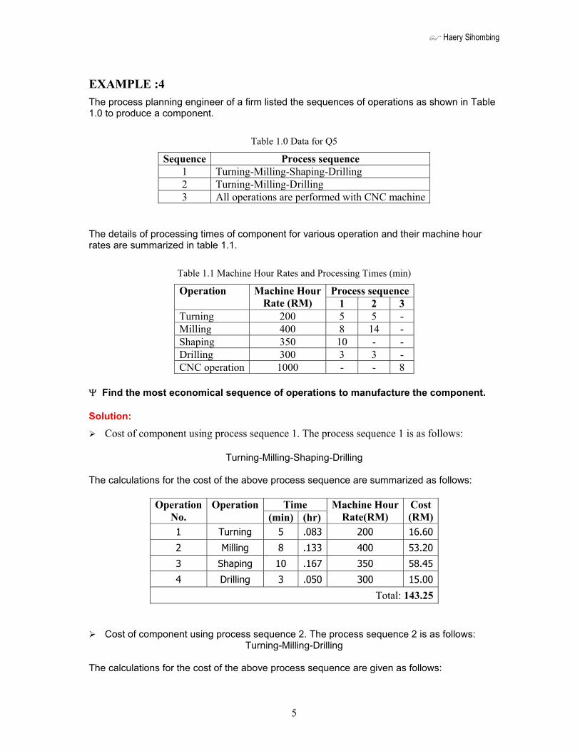
EXAMPLE :4
The process planning engineer of a firm listed the sequences of operations as shown in Table 1.0 to produce a component.
Table 1.0 Data for Q5
Sequence Process sequence
1 Turning-Milling-Shaping-Drilling
2 Turning-Milling-Drilling
3 All operations are performed with CNC machine
The details of processing times of component for various operation and their machine hour rates are summarized in table 1.1.
Table 1.1 Machine Hour Rates and Processing Times (min)
Process sequence Operation Machine Hour
Rate (RM) 1 2 3
Turning 200 5 5 -
Milling 400 8 14 -
Shaping 350 10 - -
Drilling 300 3 3 -
CNC operation 1000 - - 8
Find the most economical sequence of operations to manufacture the component.
Solution:
Cost of component using process sequence 1. The process sequence 1 is as follows:
Turning-Milling-Shaping-Drilling
The calculations for the cost of the above process sequence are summarized as follows:
TimeOperation
No.
Operation
(min) (hr)
Machine Hour
Rate(RM)
Cost
(RM)
1 Turning 5 .083 200 16.60
2 Milling 8 .133 400 53.20
3 Shaping 10 .167 350 58.45
4 Drilling 3 .050 300 15.00
Total: 143.25
Cost of component using process sequence 2. The process sequence 2 is as follows: Turning-Milling-Drilling
The calculations for the cost of the above process sequence are given as follows:

Haery Sihombing
6
TimeOperation
No.
Operation
(min) (hr)
Machine Hour
Rate(RM)
Cost
(RM)
1 Turning 5 .083 200 16.60
2 Milling 14 .233 400 93.20
3 Drilling 3 .050 300 15.00
Total:124.80
Cost of component using process sequence 3. The process sequence 3 is as follows:
TimeOperation
No.
Operation
(min) (hr)
Machine Hour
Rate(RM)
Cost
(RM)
1 CNC operations 8 .133 1000 133
The process sequence 2 has the least cost. Therefore, it should be selected for manufacturing the component.
Haery Sihombing
7
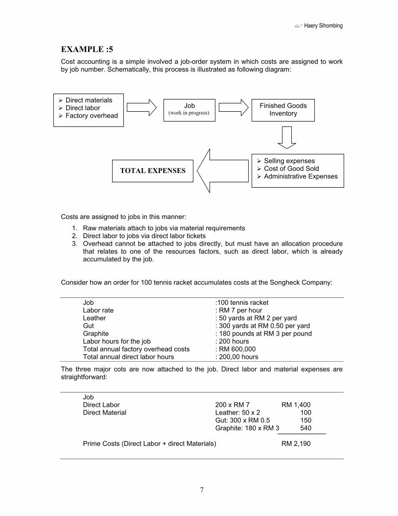
EXAMPLE :5
Cost accounting is a simple involved a job-order system in which costs are assigned to work by job number. Schematically, this process is illustrated as following diagram:
Costs are assigned to jobs in this manner:
1. Raw materials attach to jobs via material requirements 2. Direct labor to jobs via direct labor tickets 3. Overhead cannot be attached to jobs directly, but must have an allocation procedure
that relates to one of the resources factors, such as direct labor, which is already accumulated by the job.
Consider how an order for 100 tennis racket accumulates costs at the Songheck Company:
Job :100 tennis racket Labor rate : RM 7 per hour Leather : 50 yards at RM 2 per yard Gut : 300 yards at RM 0.50 per yard
Graphite : 180 pounds at RM 3 per pound Labor hours for the job : 200 hours Total annual factory overhead costs : RM 600,000 Total annual direct labor hours : 200,00 hours
The three major cots are now attached to the job. Direct labor and material expenses are straightforward:
Job Direct Labor 200 x RM 7 RM 1,400 Direct Material Leather: 50 x 2 100 Gut: 300 x RM 0.5 150 Graphite: 180 x RM 3 540
Prime Costs (Direct Labor + direct Materials) RM 2,190
Direct materials Direct labor Factory overhead
Job (work in progress)
Finished Goods Inventory
Selling expenses Cost of Good Sold Administrative Expenses
TOTAL EXPENSES

Haery Sihombing
8
Notice, that this cost is not he total cost. We must somehow find a way to attach (allocate) factory costs that cannot be directly identified to the job, but are nevertheless involved in producing the 100 rackets. Cost such as the power to run the graphite molding machine, he depreciation on this machine, the depreciation of the factory building, and the supervisor’s salary constitute overhead for this company. These overhead costs are part of the cost structure of the 100 rackets but cannot be directly traced to the job. For instance, do we really know how much machine obsolescence is attributable to the 100 rackets?
Therefore, we must allocate these overhead costs to the 100 rackets by using the overhead rate determined as follow:
Overhead rate = RM 600,000 200,000 = RM 3 per direct labor hour.
This means that RM 600 (RM 3 x 200) of the total annual overhead cost of RM 600,000 would be allocated to Job. Thus, the total cost of Job would be as follows:
Direct Labor RM 1,400 Direct Material 790 Factory Overhead 600
RM 2,790
The cost of manufacturing each racket is thus RM 27.90.
If selling expenses and administrative expenses are allocated as 40% of the cost of Goods sold, the total of a tennis racket becomes 1.4 (RM27.90) = RM 39.06
1
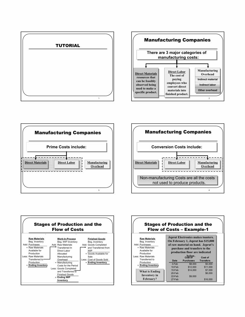
TUTORIAL
2
Manufacturing Companies
There are 3 major categories of manufacturing costs:
Direct Materials
resources that
can be feasibly
observed being
used to make a
specific product.
Direct Labor
The cost of
paying
employees who
convert direct
materials into
finished product.
Manufacturing
Overhead
Indirect material
Indirect labor
Other overhead
3
Manufacturing Companies
Prime Costs include:
Direct Materials Direct Labor Manufacturing
Overhead
4
Manufacturing Companies
Conversion Costs include:
Direct Materials Direct Labor Manufacturing
Overhead
Non-manufacturing Costs are all the costs not used to produce products.
5
Stages of Production and the
Flow of Costs
Raw Materials
Beg. Inventory
Add: Purchases
= Raw Materials
Available for
Production
Less: Raw Materials
Transferred to
Production
= Ending Inventory
Work-In-Process
Beg. WIP Inventory
Add: Raw Materials
Transferred In
Direct Labor
Allocated
Manufacturing
Overhead
= Manufacturing
Costs for the Period
Less: Goods Completed
and Transferred to
Finished Goods
= Ending WIP
Inventory
Finished Goods
Beg. Inventory
Add: Goods Completed
and Transferred from
WIP
= Goods Available for
Sale
Less: Cost of Goods Sold
= Ending Inventory
6
Stages of Production and the
Flow of Costs – Example-1
What is Ending What is Ending
Inventory in Inventory in
February?February?
Jeprut Electronics makes toasters.
On February 1, Jeprut has $15,000
of raw material on hand. Jeprut’s
purchase and transfers to the
production floor are indicated
below.
Date
Cost of
Purchases
Cost of
Transfers
3-Feb $8,000 $5,000
10-Feb $12,000 $11,000
15-Feb $14,000 $7,000
20-Feb $6,000
22-Feb $9,000
27-Feb $16,000
Raw Materials
Beg. Inventory
Add: Purchases
= Raw Materials
Available for
Production
Less: Raw Materials
Transferred to
Production
= Ending Inventory

7
Jeprut Electronics makes toasters.
On February 1, Axel has $15,000 of
raw material on hand. Jeprut ’s
purchase and transfers to the
production floor are indicated
below.below.
Date
Cost of
Purchases
Cost of
Transfers
3-Feb $8,000 $5,000
10-Feb $12,000 $11,000
15-Feb $14,000 $7,000
20-Feb $6,000
22-Feb $9,000
27-Feb $16,000
Stages of Production and the
Flow of Costs – Example-1
Now letNow let’’s look at s look at
WorkWork--inin--Process.Process.
Raw Materials
$15,000
Add: 43,000
= $58,000
Less: 45,000
= $13,000
8
Stages of Production and the
Flow of Costs – Example-1
What is the What is the
amount of cost amount of cost
transferred to transferred to
Finished Goods in Finished Goods in
February?February?
On February 1,
Jeprut had WIP of
$30,000 on the
factory floor.
During February,
Jeprut paid $92,000
in direct labor
wages. Overhead is
applied at 150% of
direct labor. On
2/28, $22,000 is still
in WIP.
Raw Materials
$15,000
Add: 43,000
= $58,000
Less: 45,000
= $13,000
Work-In-Process
Beg. WIP Inventory
Add: Raw Materials
Transferred In
Direct Labor
Allocated
Manufacturing
Overhead
= Manufacturing
Costs for the Period
Less: Goods Completed
and Transferred to
Finished Goods
= Ending WIP
Inventory
9
Stages of Production and the
Flow of Costs – Example-1
On February 1, Axel
had WIP of $30,00030,000
on the factory floor.
During February,
Jeprut paid $92,00092,000
in direct labor
wages. Overhead is
applied at 150%150% of
direct labor. On
2/28, $22,000 is still
in WIP.
Now letNow let’’ss
look at look at
FinishedFinished
Goods.Goods.
Transferred Transferred
to Finished to Finished
GoodsGoods
Work-In-Process
$30,000
Add: 45,000
92,000
138,000
= $305,000
Less: 283,000
= $22,000
Raw Materials
$15,000
Add: 43,000
= $58,000
Less: 45,000
= $13,000
10
Stages of Production and the
Flow of Costs – Example-1
On February 1, Jeprut had Finished Goods of $125,000 on hand. At the end of February, a physical inventory count
revealed $96,000 in Finished Goods still on hand.
What was Cost of Goods Sold for February?
Work-In-Process
$30,000
Add: 45,000
92,000
138,000
= $305,000
Less: 283,000
= $22,000
Raw Materials
$15,000
Add: 43,000
= $58,000
Less: 45,000
= $13,000
Finished Goods
Beg. Inventory
Add: Goods Completed
and Transferred from
WIP
= Goods Available for
Sale
Less: Cost of Goods Sold
= Ending Inventory
11
Stages of Production and the
Flow of Costs – Example-1
On February 1, Jeprut had Finished Goods of $125,000 on hand. At the end of February, a physical inventory count
revealed $96,000 in Finished Goods still on hand.
What was Cost of Goods Sold for February?
Raw Materials
$15,000
Add: 43,000
= $58,000
Less: 45,000
= $13,000
Work-In-Process
$30,000
Add: 45,000
92,000
138,000
= $305,000
Less: 283,000
= $22,000
Finished Goods
$125,000
Add: 283,000
= $408,000
Less: 312,000
= $96,000
12
Summary of Variable and Fixed Cost Behavior
Cost In Total Per Unit
Variable Total variable cost is Variable cost per unit remains
proportional to the activity the same over wide ranges
level within the relevant range. of activity.
Fixed Total fixed cost remains the Fixed cost per unit goes
same even when the activity down as activity level goes up.
level changes within the
relevant range.
Cost BehaviorFixed vs. Variable

13
Direct CostsAssigning resource costs to products and services through reliable observations and
documentation of resource use.
Some products use more of a given resource than
others.
Tracing is often more effective than using Average Cost, which assumes that each
product uses the same amount of each resource.
Traceability of Resources
14
Indirect CostsAttaching or assigning indirect costs to products,
services, or organizational units by some reasonable method of averaging.
Applied to costs that cannot be
efficiently traced.
Methods such as Activity-Based Costing result in more tracing and less
allocation.
Example
Traceability of Resources
15
Tracing versus Allocating Costs
– Example-2
Keusix makes two products; bricks and play sand. The products are produced in two separate
facilities, and the plant supervisors work at both plants. Allocate rent and salaries based on
revenues.
Keusix’s headquarters is downtown.
Product
Sales Price
per Unit
Bricks 2,000,000 0.75$
Sand 30,000 tons 90.00$
Units Produced
& Sold
16
The brick operation consumes 70% of the material purchased. The play sand uses the remaining 30%.
Labor has an average cost of $10 per hour. The brick operation uses 21,000 labor hours. The play sand
operation uses 14,000 labor hours.
The company pays all utilities on one bill that goes to the headquarters. Headquarters allocates 50% of
the utilities cost to each product.
Tracing versus Allocating Costs
– Example-2
17
Compute the missing values and information.
Tracing versus Allocating Costs
– Example-2
Cost Type Total Cost Bricks Sand
How
Assigned
Sales Revenue 4,200,000$ ? ? ?
Materials 800,000 ? ? ?
Labor 350,000 ? ? ?
Supervisors 140,000 ? ? ?
Plant Rent 700,000 ? ? ?
Total Utilities 160,000 ? ? ?
18
Sales Revenue is TRACED to each product based on the actual revenue each product generates.
Example: Sand Revenue = 30,000 tons × $90 per ton
Cost Type Total Cost Bricks Sand
How
Assigned
Sales Revenue 4,200,000$ 1,500,000$ 2,700,000$ Direct
Materials 800,000 ? ? ?
Labor 350,000 ? ? ?
Supervisors 140,000 ? ? ?
Plant Rent 700,000 ? ? ?
Total Utilities 160,000 ? ? ?
Tracing versus Allocating Costs
– Example-2

19
Tracing versus Allocating Costs
– Example-2
Material and Labor are traced to each product based on how much of each resource each product uses.
Example; Bricks labor = 21,000 hours × $10 per hour
Cost Type Total Cost Bricks Sand
How
Assigned
Sales Revenue 4,200,000$ 1,500,000$ 2,700,000$ Direct
Materials 800,000 560,000$ 240,000$ Direct
Labor 350,000 210,000$ 140,000$ Direct
Supervisors 140,000 ? ? ?
Plant Rent 700,000 ? ? ?
Total Utilities 160,000 ? ? ?
20
Tracing versus Allocating Costs
– Example-2
Supervisor salaries and rent are allocated on the basis of relative revenues. Approximately 35.7% goes to
Bricks. Approximately 64.3% goes to Sand.
Cost Type Total Cost Bricks Sand
How
Assigned
Sales Revenue 4,200,000$ 1,500,000$ 2,700,000$ Direct
Materials 800,000 560,000$ 240,000$ Direct
Labor 350,000 210,000$ 140,000$ Direct
Supervisors 140,000 50,000$ 90,000$ Indirect
Plant Rent 700,000 250,000$ 450,000$ Indirect
Total Utilities 160,000 ? ? ?
21
Cost Type Total Cost Bricks Sand
How
Assigned
Sales Revenue 4,200,000$ 1,500,000$ 2,700,000$ Direct
Materials 800,000 560,000$ 240,000$ Direct
Labor 350,000 210,000$ 140,000$ Direct
Supervisors 140,000 50,000$ 90,000$ Indirect
Plant Rent 700,000 250,000$ 450,000$ Indirect
Total Utilities 160,000 80,000$ 80,000$ Indirect
The utilities are allocated from the home office with 50% of the utilities being charged to each product.
Tracing versus Allocating Costs
– Example-2
22
Variable Costingmeasures product cost by the unit-level resources
used.
Absorption Costingallocates indirect costs to products
along with unit-level and variable costs.
Income-Reporting Effects of
Alternative Product-Costing Methods
23
Overview of Absorption and Variable Costing
Direct Materials
Direct Labor
Variable Manufacturing Overhead
Fixed Manufacturing Overhead
Variable Selling and Administrative Expenses
Fixed Selling and Administrative Expenses
Variable
Costing
Absorption
Costing
Product
Costs
Period
Costs
Product
Costs
Period
Costs
24
Absorption
Costing
Variable
Costing
Direct materials
Direct labor Product costs
Product costs Variable mfg. overhead
Fixed mfg. overhead
Period costs
Period costs Selling & admin. exp.
Income-Reporting Effects of
Alternative Product-Costing Methods

25
Absorption Costing vs. Variable Costing –
Example-3
Bemo, Inc. produces a single product with a sales price of $40 and the following cost information:
Number of units produced annually 30,000
Variable costs per unit:
Direct materials, direct labor,
and variable mfg. overhead 12$
Selling & administrative expenses 4$
Fixed costs per year:
Manufacturing overhead 210,000$
Selling & administrative expenses 250,000$
Number of units produced annually 30,000
Variable costs per unit:
Direct materials, direct labor,
and variable mfg. overhead 12$
Selling & administrative expenses 4$
Fixed costs per year:
Manufacturing overhead 210,000$
Selling & administrative expenses 250,000$
26
Unit product cost is determined as follows:
Selling and administrative expenses arealways treated as period expenses and deducted from
revenue.
Absorption
Costing
Variable
Costing
Direct materials, direct labor,
and variable mfg. overhead 12$ 12$
Fixed mfg. overhead
($210,000 ÷ 30,000 units) 7 -
Unit product cost 19$ 12$
Absorption Costing vs. Variable Costing –
Example-3
27
Absorption CostingSales (28,000 × $40) 1,120,000$
Less cost of goods sold:
Beginning inventory -$
Add COGM (30,000 × $19) 570,000
Goods available for sale 570,000
Ending inventory (2,000 × $19) 38,000 532,000
Gross margin 588,000
Less selling & admin. exp.
Variable (28,000 x $4) 112,000$
Fixed 250,000 362,000
Net income 226,000$
Bemo, Inc. had no beginning inventory, produced30,000 units and sold 28,000 units this year.
Absorption Costing vs. Variable Costing –
Example-3
28
Variable CostingSales (28,000 × $40) 1,120,000$
Less variable expenses:
Beginning inventory -$
Add COGM (30,000 × $12) 360,000
Goods available for sale 360,000
Ending inventory (2,000 × $12) 24,000
Variable cost of goods sold 336,000
Variable selling & administrative
expenses (28,000 × $4) 112,000 448,000
Contribution margin 672,000
Less fixed expenses:
Manufacturing overhead 210,000$
Selling & administrative expenses 250,000 460,000
Net income 212,000$
Variablecostsonly.
All fixedmanufacturing
overhead isexpensed.
Absorption Costing vs. Variable Costing –
Example-3
29
Olenk Company produces a single productwith the following information available:
Number of units produced annually 25,000
Variable costs per unit:
Direct materials, direct labor,
and variable mfg. overhead 10$
Selling & administrative expenses 3$
Fixed costs per year:
Manufacturing overhead 150,000$
Selling & administrative expenses 100,000$
Number of units produced annually 25,000
Variable costs per unit:
Direct materials, direct labor,
and variable mfg. overhead 10$
Selling & administrative expenses 3$
Fixed costs per year:
Manufacturing overhead 150,000$
Selling & administrative expenses 100,000$
Absorption Costing vs. Variable Costing –
Example-4
30
Unit product cost is determined as follows:
Selling and administrative expenses arealways treated as period expenses and deducted from
revenue as incurred.
Absorption
Costing
Variable
Costing
Direct materials, direct labor,
and variable mfg. overhead 10$ 10$
Fixed mfg. overhead
($150,000 ÷ 25,000 units) 6 -
Unit product cost 16$ 10$
Absorption
Costing
Variable
Costing
Direct materials, direct labor,
and variable mfg. overhead 10$ 10$
Fixed mfg. overhead
($150,000 ÷ 25,000 units) 6 -
Unit product cost 16$ 10$
Absorption Costing vs. Variable Costing –
Example-4

31
Income Comparison ofAbsorption and Variable Costing
Let’s assume the following additional information for Olenk Company.
• 20,000 units were sold during the year at a price of $30 each.
• There were no units in beginning inventory.
Now, let’s compute net operatingincome using both absorptionand variable costing.
32
Absorption CostingSales (20,000 × $30) 600,000$
Less cost of goods sold:
Beginning inventory -$
Add COGM (25,000 × $16) 400,000
Goods available for sale 400,000
Ending inventory (5,000 × $16) 80,000 320,000
Gross margin 280,000
Less selling & admin. exp.
Variable (20,000 × $3) 60,000$
Fixed 100,000 160,000
Net operating income 120,000$
Absorption CostingExample-5
33
Variable CostingSales (20,000 × $30) 600,000$
Less variable expenses:
Beginning inventory -$
Add COGM (25,000 × $10) 250,000
Goods available for sale 250,000
Less ending inventory (5,000 × $10) 50,000
Variable cost of goods sold 200,000
Variable selling & administrative
expenses (20,000 × $3) 60,000 260,000
Contribution margin 340,000
Less fixed expenses:
Manufacturing overhead 150,000$
Selling & administrative expenses 100,000 250,000
Net operating income 90,000$
Variablemanufacturing
costs only.
All fixedmanufacturing
overhead isexpensed.
Variable Costing
34
Cost of
Goods
Sold
Ending
Inventory
Period
Expense Total
Absorption costing
Variable mfg. costs 200,000$ 50,000$ -$ 250,000$
Fixed mfg. costs 120,000 30,000 - 150,000
320,000$ 80,000$ -$ 400,000$
Variable costing
Variable mfg. costs 200,000$ 50,000$ -$ 250,000$
Fixed mfg. costs - - 150,000 150,000
200,000$ 50,000$ 150,000$ 400,000$
Income Comparison ofAbsorption and Variable Costing
Let’s compare the methods.
35
Reconciliation
Variable costing net operating income 90,000$
Add: Fixed mfg. overhead costs
deferred in inventory
(5,000 units × $6 per unit) 30,000
Absorption costing net operating income 120,000$
Variable costing net operating income 90,000$
Add: Fixed mfg. overhead costs
deferred in inventory
(5,000 units × $6 per unit) 30,000
Absorption costing net operating income 120,000$
Fixed mfg. Overhead $150,000 Units produced 25,000 units
= = $6.00 per unit
We can reconcile the difference betweenabsorption and variable income as follows:
36
Extended Comparison of Income Data Olenk Company Year Two
Number of units produced 25,000
Number of units sold 30,000
Units in beginning inventory 5,000
Unit sales price 30$
Variable costs per unit:
Direct materials, direct labor
variable mfg. overhead 10$
Selling & administrative
expenses 3$
Fixed costs per year:
Manufacturing overhead 150,000$
Selling & administrative
expenses 100,000$

37
Unit Cost Computations
Since there was no change in the variable costsper unit, total fixed costs, or the number of
units produced, the unit costs remain unchanged.
Absorption
Costing
Variable
Costing
Direct materials, direct labor,
and variable mfg. overhead 10$ 10$
Fixed mfg. overhead
($150,000 ÷ 25,000 units) 6 -
Unit product cost 16$ 10$
Absorption
Costing
Variable
Costing
Direct materials, direct labor,
and variable mfg. overhead 10$ 10$
Fixed mfg. overhead
($150,000 ÷ 25,000 units) 6 -
Unit product cost 16$ 10$
38
Absorption CostingSales (30,000 × $30) 900,000$
Less cost of goods sold:
Beg. inventory (5,000 × $16) 80,000$
Add COGM (25,000 × $16) 400,000
Goods available for sale 480,000
Less ending inventory - 480,000
Gross margin 420,000
Less selling & admin. exp.
Variable (30,000 × $3) 90,000$
Fixed 100,000 190,000
Net operating income 230,000$
Absorption Costing
These are the 25,000 unitsproduced in the current period.
39
Variable CostingSales (30,000 × $30) 900,000$
Less variable expenses:
Beg. inventory (5,000 × $10) 50,000$
Add COGM (25,000 × $10) 250,000
Goods available for sale 300,000
Less ending inventory -
Variable cost of goods sold 300,000
Variable selling & administrative
expenses (30,000 × $3) 90,000 390,000
Contribution margin 510,000
Less fixed expenses:
Manufacturing overhead 150,000$
Selling & administrative expenses 100,000 250,000
Net operating income 260,000$
Variable Costing
All fixedmanufacturing
overhead isexpensed.
Variablemanufacturing
costs only.
40
Reconciliation
Variable costing net operating income 260,000$
Deduct: Fixed manufacturing overhead
costs released from inventory
(5,000 units × $6 per unit) 30,000
Absorption costing net operating income 230,000$
We can reconcile the difference betweenabsorption and variable income as follows:
Fixed mfg. Overhead $150,000 Units produced 25,000 units
= = $6.00 per unit
41
Income Comparison
Costing Method 1st Period 2nd Period Total
Absorption 120,000$ 230,000$ 350,000$
Variable 90,000 260,000 350,000
42
Summary
Relation between Effect Relation between
production on variable and
and sales inventory absorption income
Inventory Absorption
Production > Sales increases >
Variable
Inventory Absorption
Production < Sales decreases <
Variable
Absorption
Production = Sales No change =
Variable

43
Impact on the Manager
Opponents of absorption costing argue that shiftingfixed manufacturing overhead costs between periodscan lead to misinterpretations and faulty decisions.
Those who favor variable costing argue that the incomestatements are easier to understand because net operating
income is only affected by changes in unit sales. Theresulting income amounts are more consistent with
managers’ expectations.