Embed Size (px)
Citation preview

1
Hybrid Intelligent Systems
Lecture 4 - Part A
Evolutionary Neural NetworksEvolving Fuzzy Systems
Hybrid Intelligent Systems
Lecture 4 - Part A
Evolutionary Neural NetworksEvolving Fuzzy Systems
2
Artificial Neural Networks - FeaturesArtificial Neural Networks - Features
• Typically, structure of a neural network is established and one of a variety of mathematical algorithms is used to determine what the weights of the interconnections should be to maximize the accuracy of the outputs produced.
• This process by which the synaptic weights of a neural network are adapted according to the problem environment is popularly known as learning.
• There are broadly three types of learning: Supervised learning, unsupervised learning and reinforcement learning
3
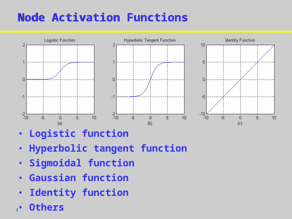
Node Activation FunctionsNode Activation Functions
• Logistic function
• Hyperbolic tangent function
• Sigmoidal function
• Gaussian function
• Identity function
• Others
4
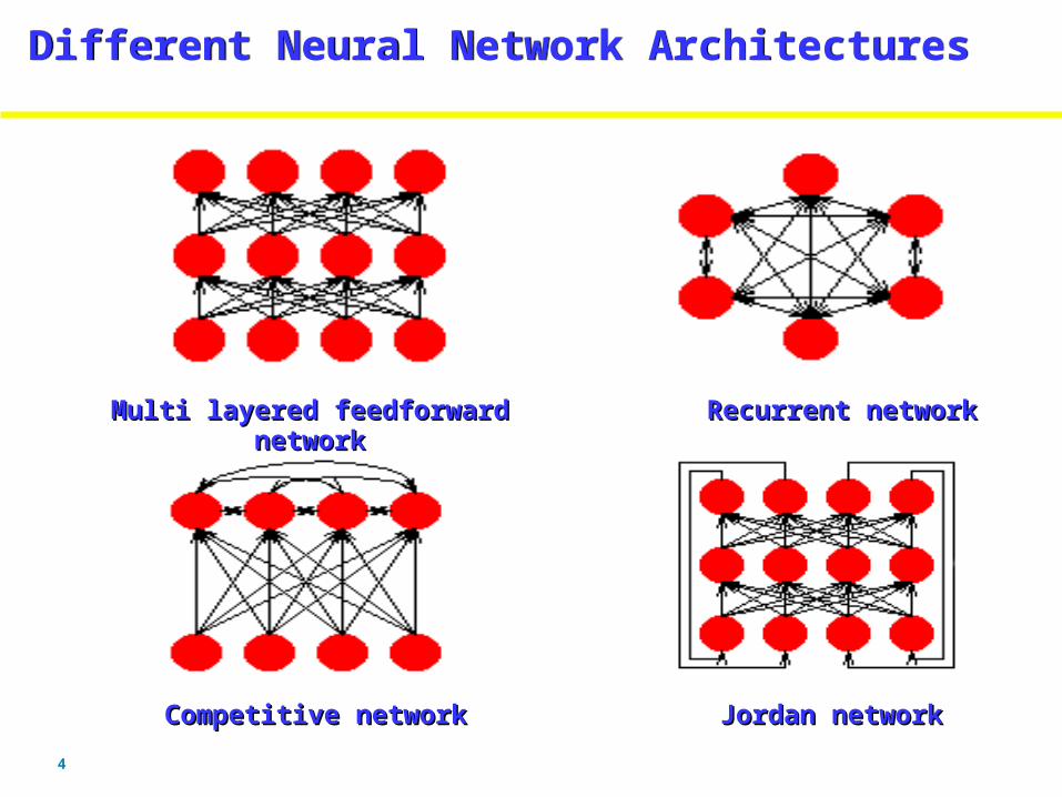
Different Neural Network ArchitecturesDifferent Neural Network Architectures
Multi layered feedforward networkMulti layered feedforward network Recurrent networkRecurrent network
Competitive networkCompetitive network Jordan networkJordan network

5
Backpropagation AlgorithmBackpropagation AlgorithmBackpropagation AlgorithmBackpropagation Algorithm
Backpropagation algorithm
1)(nΔw*αδw
δE*ε(n)Δw ij
ijij
• E = error criteria to be minimized
• wij = weight from the i-th input unit to the j-th output
• and are the learning rate and momentum
6
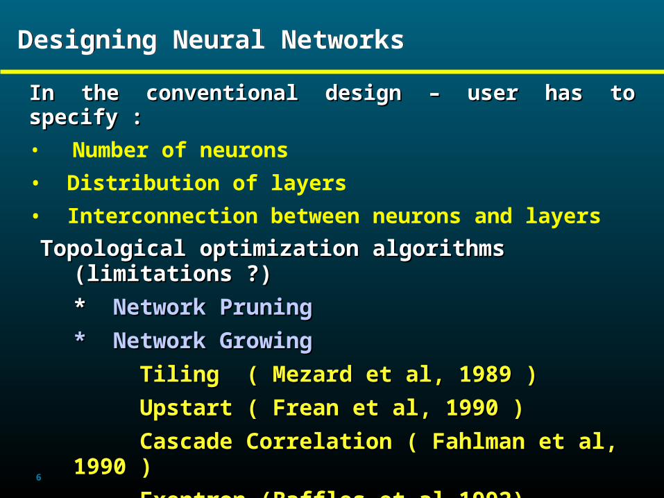
Designing Neural NetworksDesigning Neural Networks
In the conventional design – user has to specify :In the conventional design – user has to specify :
• Number of neurons
• Distribution of layers
• Interconnection between neurons and layers
Topological optimization algorithms (limitations ?) Topological optimization algorithms (limitations ?)
* * Network PruningNetwork Pruning
* Network Growing* Network Growing
Tiling ( Mezard et al, 1989 )Tiling ( Mezard et al, 1989 )
Upstart ( Frean et al, 1990 )Upstart ( Frean et al, 1990 )
Cascade Correlation ( Fahlman et al, 1990 )Cascade Correlation ( Fahlman et al, 1990 )
Exentron (Baffles et al 1992)Exentron (Baffles et al 1992)

7
Choosing Hidden NeuronsChoosing Hidden NeuronsChoosing Hidden NeuronsChoosing Hidden Neurons
A large number of hidden neurons will ensure the correct learning and the network is able to correctly predict the data it has been trained on, but its performance on new data, its ability to generalise, is compromised.
With too few a hidden neurons, the network may be unable to learn the relationships amongst the data and the error will fail to fall below an acceptable level.
Selection of the number of hidden neurons is a crucial decision.
Often a trial and error approach is taken.
8
Choosing Initial WeightsChoosing Initial WeightsChoosing Initial WeightsChoosing Initial Weights
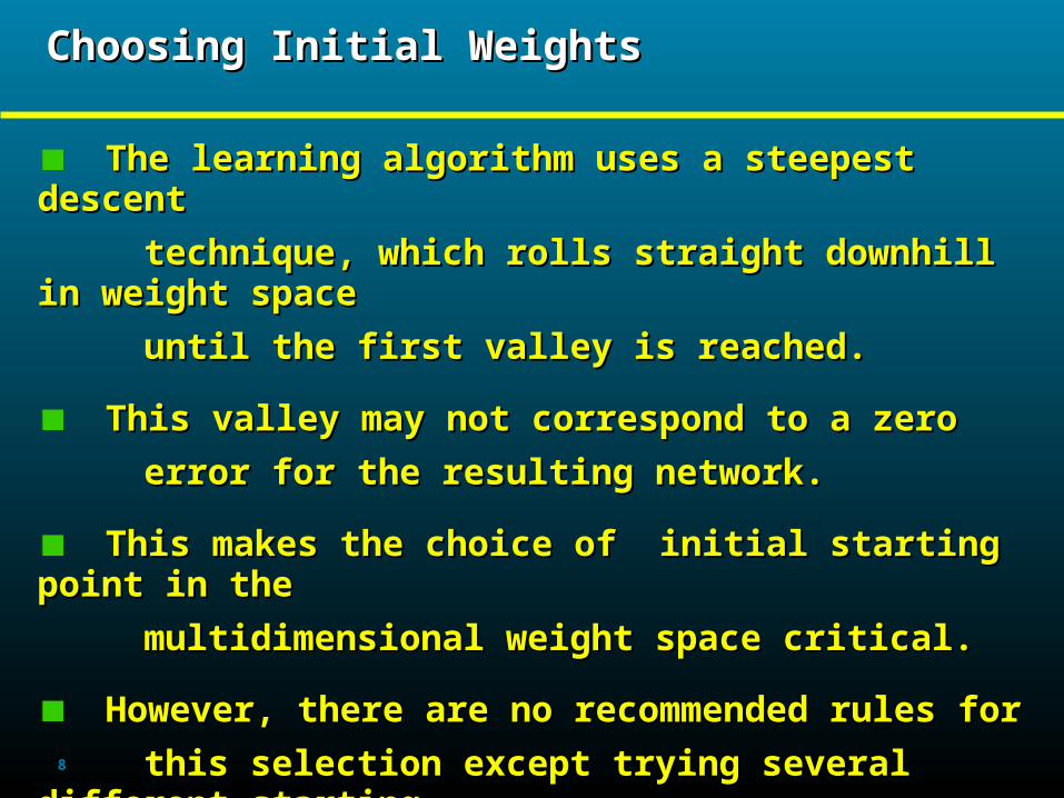
The learning algorithm uses a steepest descent The learning algorithm uses a steepest descent
technique, which rolls straight downhill in technique, which rolls straight downhill in weight space weight space
until the first valley is reached. until the first valley is reached.
This valley may not correspond to a zero This valley may not correspond to a zero
error for the resulting network. error for the resulting network.
This makes the choice of initial starting point This makes the choice of initial starting point in the in the
multidimensional weight space critical. multidimensional weight space critical.
However, there are no recommended rules for However, there are no recommended rules for
this selection except trying several different this selection except trying several different starting starting
weight values to see if the network results are weight values to see if the network results are improved.improved.
9
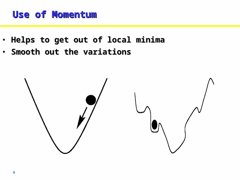
Use of MomentumUse of MomentumUse of MomentumUse of Momentum
• Helps to get out of local minimaHelps to get out of local minima
• Smooth out the variationsSmooth out the variations
10
Choosing the learning rateChoosing the learning rateChoosing the learning rateChoosing the learning rate
Learning rate controls the size of the step that Learning rate controls the size of the step that is taken in is taken in multidimensional weight space when each multidimensional weight space when each weight is weight is modified.modified.
If the selected learning rate is too large then If the selected learning rate is too large then the local the local minimum may be overstepped constantly, minimum may be overstepped constantly, resulting in resulting in oscillations and slow convergence to the lower oscillations and slow convergence to the lower error error state.state.
If the learning rate is too low, the number of If the learning rate is too low, the number of iterations iterations required may be too large, resulting in slow required may be too large, resulting in slow performance. performance.
11
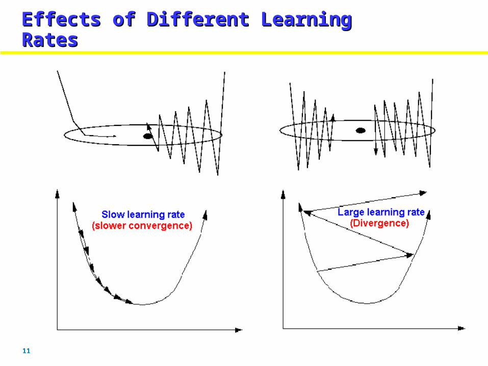
Effects of Different Learning RatesEffects of Different Learning RatesEffects of Different Learning RatesEffects of Different Learning Rates

12
Gradient Descent PerformanceGradient Descent PerformanceGradient Descent PerformanceGradient Descent Performance
Trapped in local Trapped in local minimaminima
Desired behaviorDesired behavior
Undesired behaviorUndesired behavior
13
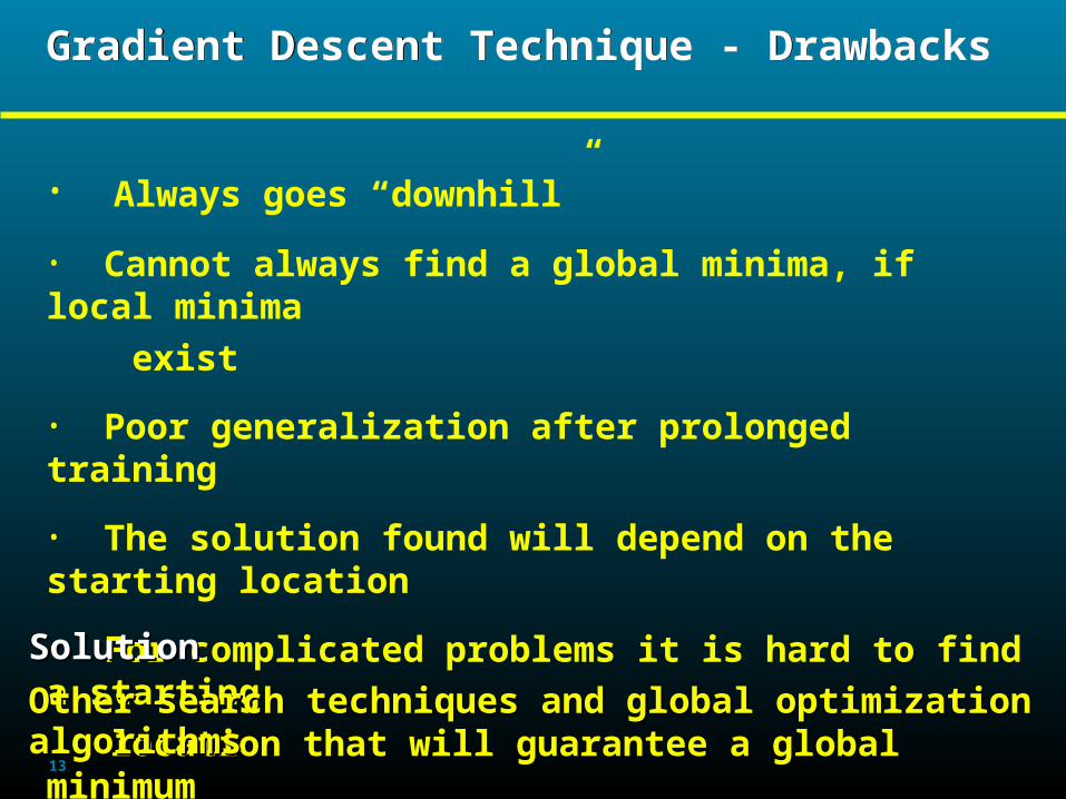
Gradient Descent Technique - Drawbacks Gradient Descent Technique - Drawbacks
• Always goes “downhill”
• Cannot always find a global minima, if local minima exist
• Poor generalization after prolonged training
• The solution found will depend on the starting location
• For complicated problems it is hard to find a starting location that will guarantee a global minimum
SolutionSolution
Other search techniques and global optimization algorithms Other search techniques and global optimization algorithms

14
Conjugate Gradient AlgorithmsConjugate Gradient AlgorithmsConjugate Gradient AlgorithmsConjugate Gradient Algorithms
Search is performed in conjugate directions
• Start with the steepest descent (first iteration)
• Line search to move along the current direction
• New search direction is conjugate to previous
direction ( new steepest search direction + previous
search direction)
• Fletcher - Reeves Update
• Polak - Ribiere Update
• Powelle - Beale Restart
• Scaled Conjugate Algorithm
1kkkk pβgp

15
Scaled Conjugate Gradient Algorithm Scaled Conjugate Gradient Algorithm
• SCGA avoids the complicated line search procedure
of conventional conjugate gradient algorithm
kpkk
)kw('E)kpkkw(
'Ekp)kw(
"E
Hessian
Matrix
E' and E" are the first and second derivative information
Pk = search direction
σ k = change in weight for second derivative
λk = regulating indefiniteness of the Hessian For a good quadratic approximation of E, a mechanism to raise and lower λk is needed when the Hessian is positive definite. Initial values of σ k and λk is important.
16
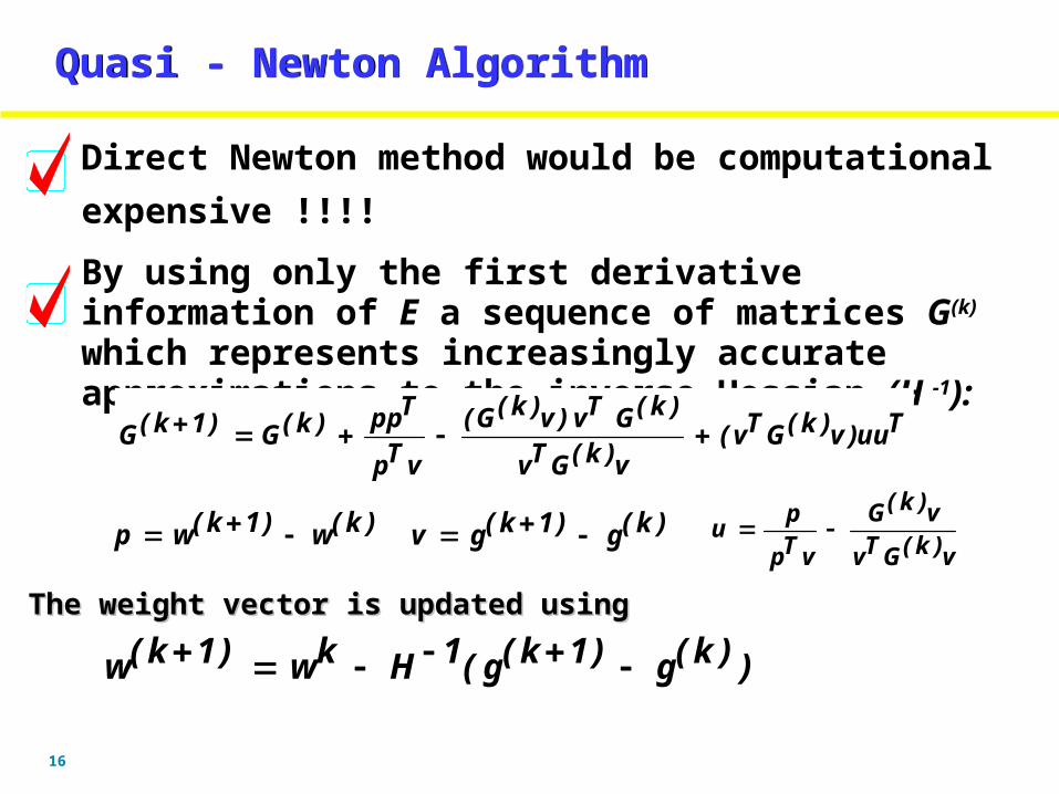
Quasi - Newton AlgorithmQuasi - Newton Algorithm
By using only the first derivative information of E a sequence of matrices G(k) which represents increasingly accurate approximations to the inverse Hessian (H -1):
Tuu)v)k(GTv(v)k(GTv
)k(GTv)v)k(G(
vTp
Tpp)k(G)1k(G
)k(w)1k(wp )k(g)1k(gv v)k(GTv
v)k(G
vTp
pu
Direct Newton method would be computational
expensive !!!!
The weight vector is updated usingThe weight vector is updated using
))k(g)1k(g(1Hkw)1k(w
17
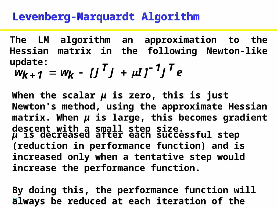
Levenberg-Marquardt AlgorithmLevenberg-Marquardt Algorithm
The LM algorithm an approximation to the Hessian matrix in the following Newton-like update:
eTJ1]IJTJ[kw1kw
μ is decreased after each successful step (reduction in performance function) and is increased only when a tentative step would increase the performance function.
By doing this, the performance function will always be reduced at each iteration of the algorithm
When the scalar μ is zero, this is just Newton's method, using the approximate Hessian matrix. When μ is large, this becomes gradient descent with a small step size.
18
Limitations of Conventional Design of Neural NetsLimitations of Conventional Design of Neural Nets
• What is the optimal architecture for a given
problem (no of neurons and no of hidden layers) ?
• What activation function should one choose?
• What is the optimal learning algorithm and its
parameters?
To demonstrate the difficulties in designing “optimal” neural networks we will consider three famous time series benchmark problems ! (Reference 4)
19
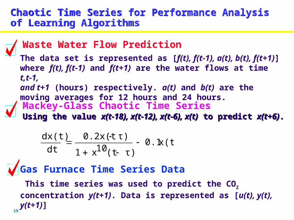
Chaotic Time Series for Performance Analysis of Learning AlgorithmsChaotic Time Series for Performance Analysis of Learning Algorithms
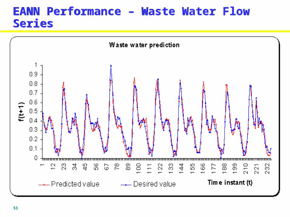
Waste Water Flow Prediction
The data set is represented as [f(t), f(t-1), a(t), b(t), f(t+1)] where f(t), f(t-1) and f(t+1) are the water flows at time t,t-1, and t+1 (hours) respectively. a(t) and b(t) are the moving averages for 12 hours and 24 hours. Mackey-Glass Chaotic Time SeriesUsing the value Using the value x(t-18), x(t-12), x(t-6), x(t)x(t-18), x(t-12), x(t-6), x(t) to predict to predict x(t+6)x(t+6)..
x(t)0.1τ)(t10x1
τ)0.2x(t
dt
dx(t)
Gas Furnace Time Series Data This time series was used to predict the CO2
concentration y(t+1). Data is represented as [u(t), y(t), y(t+1)]
20
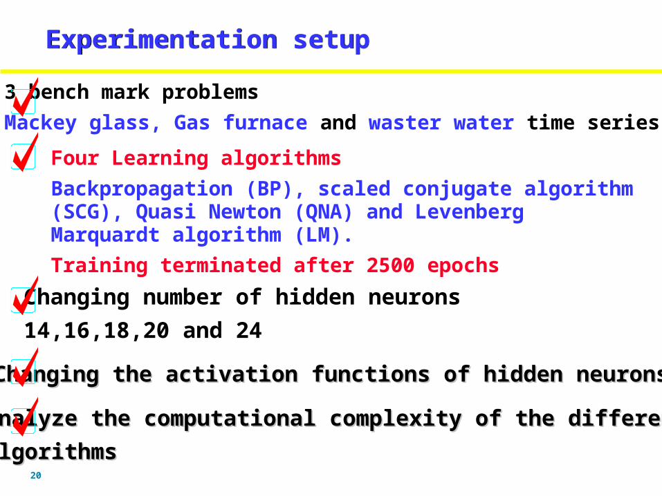
Experimentation setupExperimentation setup
Changing number of hidden neurons
14,16,18,20 and 24
3 bench mark problems
Mackey glass, Gas furnace and waster water time series
Four Learning algorithms
Backpropagation (BP), scaled conjugate algorithm (SCG), Quasi Newton (QNA) and Levenberg Marquardt algorithm (LM).
Training terminated after 2500 epochs
Changing the activation functions of hidden neuronsChanging the activation functions of hidden neurons
Analyze the computational complexity of the different Analyze the computational complexity of the different
algorithmsalgorithms
21
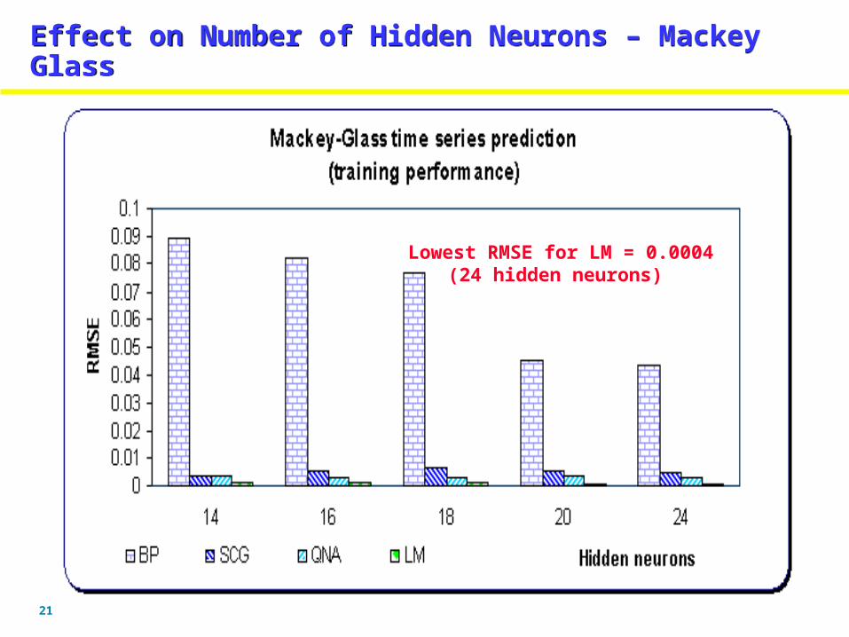
Effect on Number of Hidden Neurons – Mackey GlassEffect on Number of Hidden Neurons – Mackey Glass
Lowest RMSE for LM = 0.0004(24 hidden neurons)
22
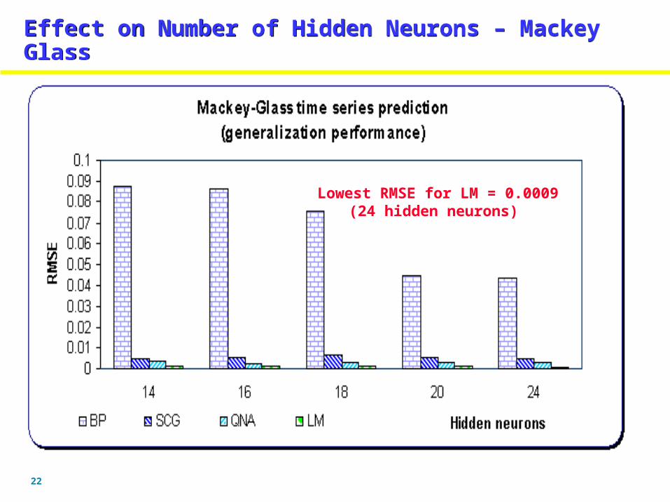
Effect on Number of Hidden Neurons – Mackey GlassEffect on Number of Hidden Neurons – Mackey Glass
Lowest RMSE for LM = 0.0009(24 hidden neurons)

23
Effect on Number of Hidden Neurons - Gas Furnace SeriesEffect on Number of Hidden Neurons - Gas Furnace Series
Lowest RMSE for LM = 0.009(24 hidden neurons)
24
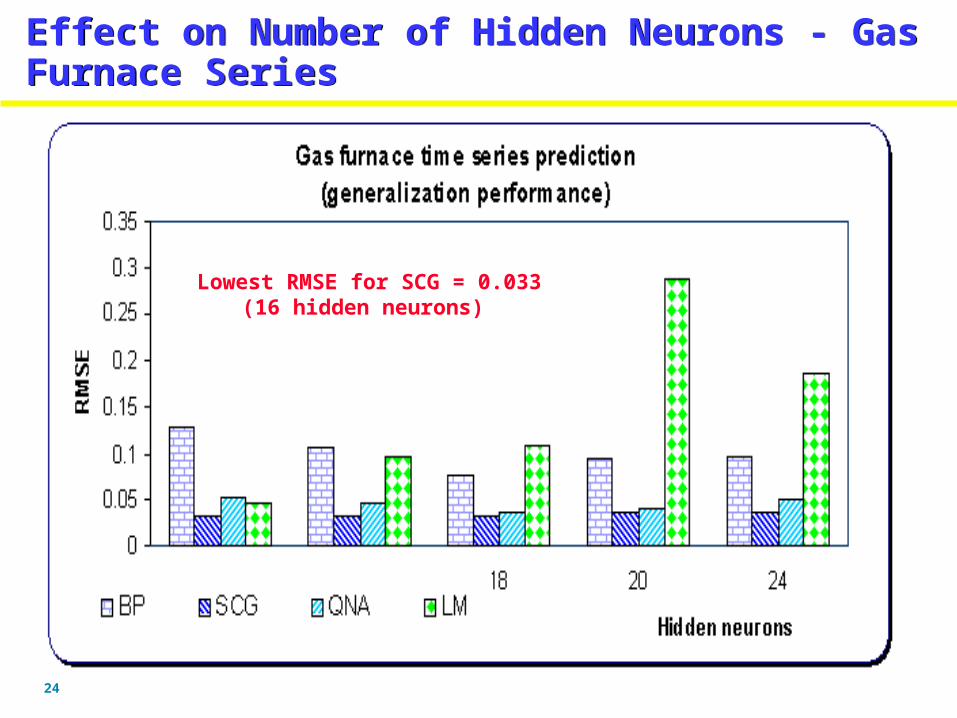
Effect on Number of Hidden Neurons - Gas Furnace SeriesEffect on Number of Hidden Neurons - Gas Furnace Series
Lowest RMSE for SCG = 0.033(16 hidden neurons)

25
Effect on Number of Hidden Neurons - Waste WaterEffect on Number of Hidden Neurons - Waste Water
Lowest RMSE for LM = 0.024(24 hidden neurons)
26
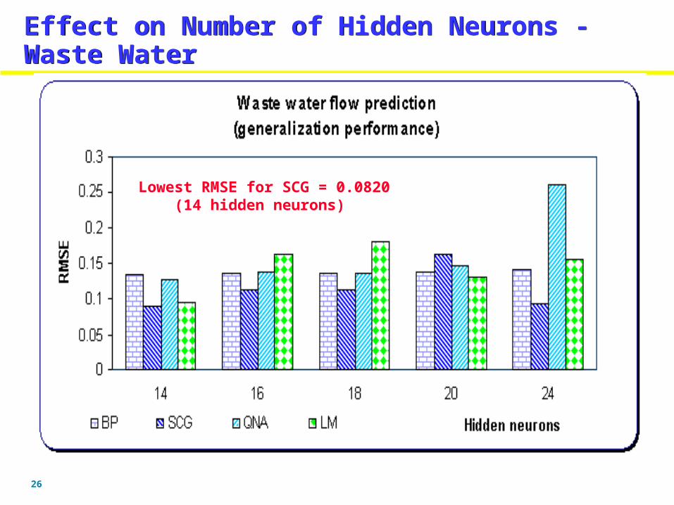
Effect on Number of Hidden Neurons - Waste WaterEffect on Number of Hidden Neurons - Waste Water
Lowest RMSE for SCG = 0.0820(14 hidden neurons)
27
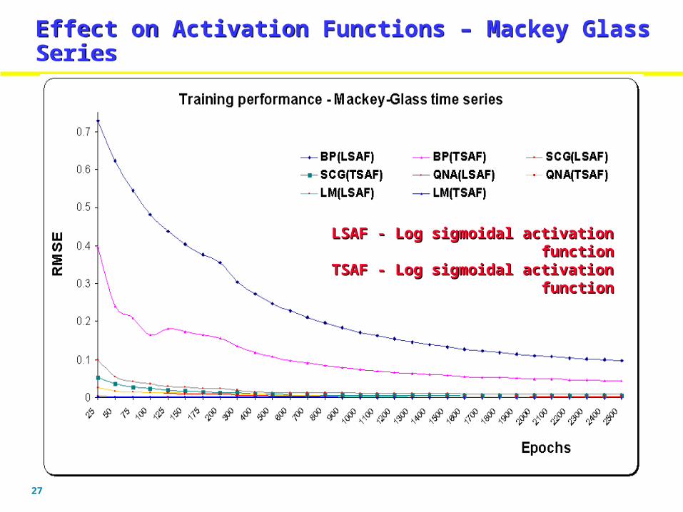
Effect on Activation Functions – Mackey Glass SeriesEffect on Activation Functions – Mackey Glass Series
LSAF - Log sigmoidal activation functionLSAF - Log sigmoidal activation functionTSAF - Log sigmoidal activation functionTSAF - Log sigmoidal activation function
28
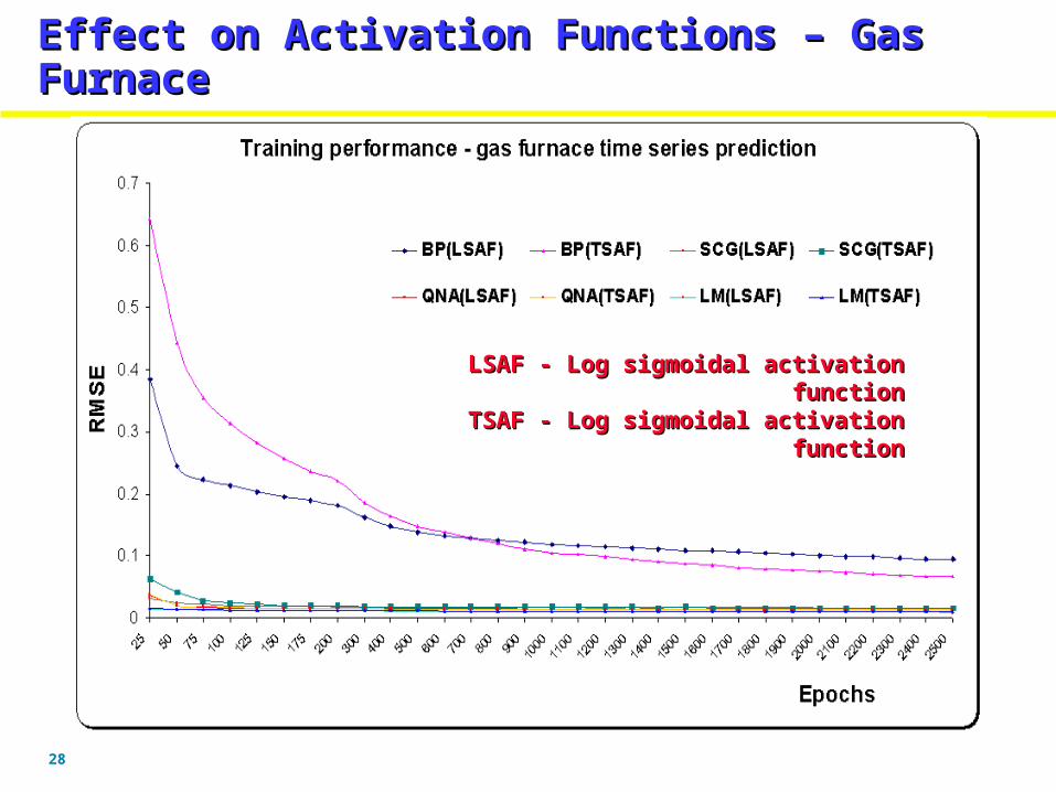
Effect on Activation Functions – Gas Effect on Activation Functions – Gas FurnaceFurnaceEffect on Activation Functions – Gas Effect on Activation Functions – Gas FurnaceFurnace
LSAF - Log sigmoidal activation functionLSAF - Log sigmoidal activation functionTSAF - Log sigmoidal activation functionTSAF - Log sigmoidal activation function
29
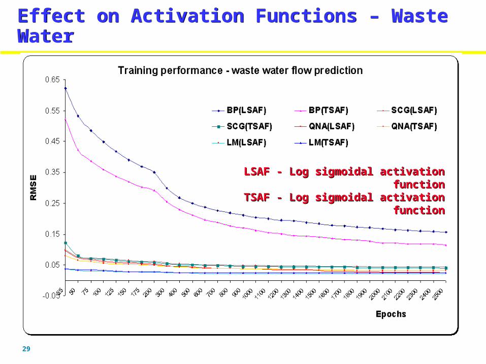
Effect on Activation Functions – Waste WaterEffect on Activation Functions – Waste Water
LSAF - Log sigmoidal activation functionLSAF - Log sigmoidal activation functionTSAF - Log sigmoidal activation functionTSAF - Log sigmoidal activation function
30
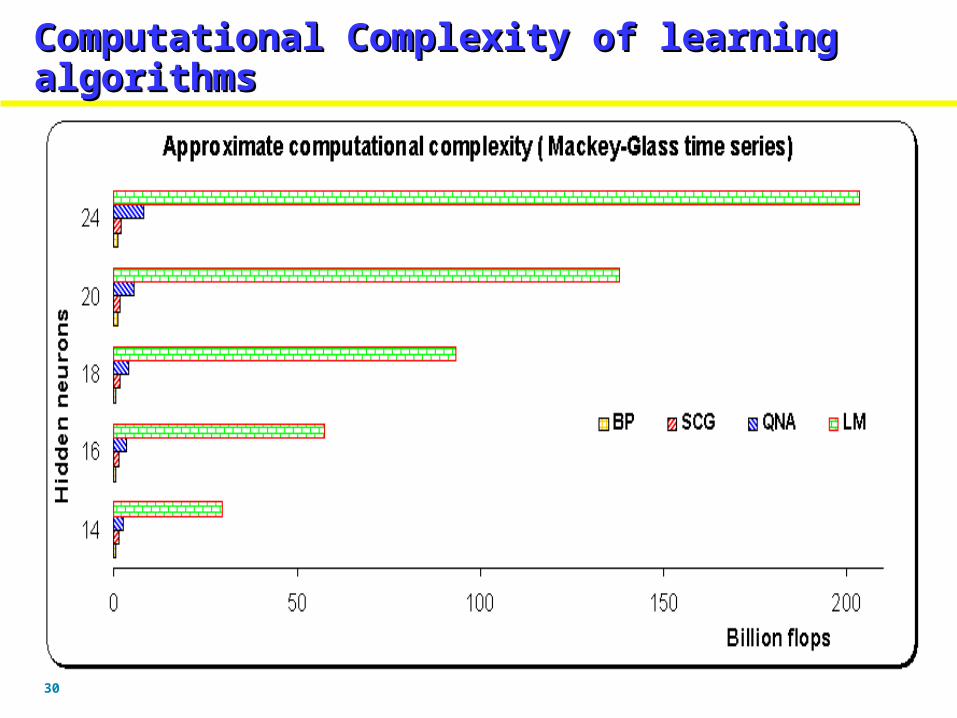
Computational Complexity of learning Computational Complexity of learning algorithmsalgorithmsComputational Complexity of learning Computational Complexity of learning algorithmsalgorithms
31
Difficulties to Design Optimal Neural Networks ?Difficulties to Design Optimal Neural Networks ?
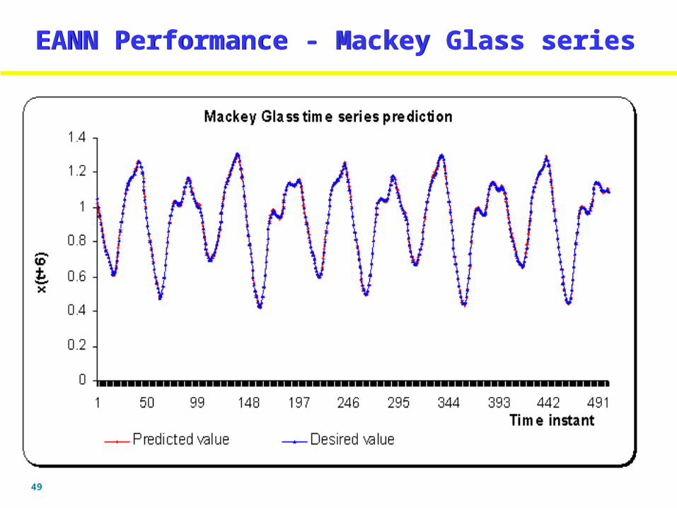
Experiments highlight the difficulty in finding an OPTIMAL network which is smaller in size, faster in convergence and with the best generalization error. For Mackey Glass series LM gave the lowest generalization RMSE of 0.0009 with 24 hidden neurons using TSAFusing TSAF
For gas furnace series the best RMSE For gas furnace series the best RMSE generalization performance was obtained using generalization performance was obtained using SCG ( 0.033) using 16 neurons and TSAF. QNA SCG ( 0.033) using 16 neurons and TSAF. QNA gave marginally better generalization error when gave marginally better generalization error when the activation function was changed from TSAF the activation function was changed from TSAF to LSAF to LSAF

32
Difficulties to Design Optimal Neural Networks ?Difficulties to Design Optimal Neural Networks ?
For wastewater series the best RMSE generalization performance was obtained using SCG (0.09) using TSAF. SCG's generalization error was improved (0.082) when the activation function was changed from TSAF to LSAF. In spite of computational complexity, LM performed well for Mackey Glass. For gas furnace and wastewater SCG algorithm performed better.
This leads us to the following questions: What is the optimal architecture for a given problem? What activation function should one choose? What is the optimal learning algorithm and its parameters?Solution : Solution : Optimizing Artificial Neural Networks Using Optimizing Artificial Neural Networks Using Global Optimization AlgorithmsGlobal Optimization Algorithms
33
Global Optimization AlgorithmsGlobal Optimization Algorithms
• No need for functional derivative information No need for functional derivative information
• Repeated evaluations of objective functionsRepeated evaluations of objective functions
• Intuitive guidelines (simplicity)Intuitive guidelines (simplicity)
• RandomnessRandomness
• Analytic opacityAnalytic opacity
• Self optimizationSelf optimization
• Ability to handle complicated tasksAbility to handle complicated tasks
• Broad applicability Broad applicability
DisadvantageDisadvantage
Computational expensive Computational expensive (use parallel engines)(use parallel engines)
34
Popular Global Optimization AlgorithmsPopular Global Optimization AlgorithmsPopular Global Optimization AlgorithmsPopular Global Optimization Algorithms
Genetic algorithmsGenetic algorithms
Simulated annealingSimulated annealing
Tabu searchTabu search
Random searchRandom search
Down hill simplex searchDown hill simplex search
GRASPGRASP
Clustering methods Clustering methods
Many othersMany others
35
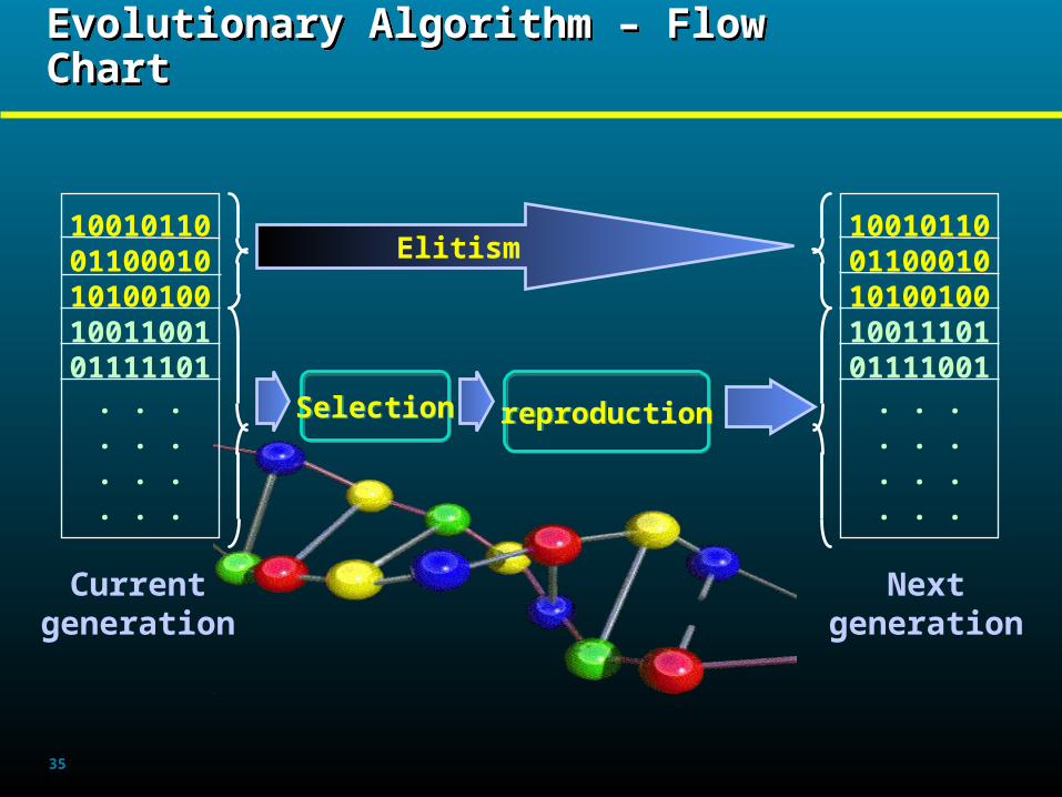
Evolutionary Algorithm – Flow ChartEvolutionary Algorithm – Flow Chart
1001011001100010101001001001100101111101
. . .
. . .
. . .
. . .
1001011001100010101001001001110101111001
. . .
. . .
. . .
. . .
SelectionSelection reproductionreproduction
Currentgeneration
Nextgeneration
Elitism
36
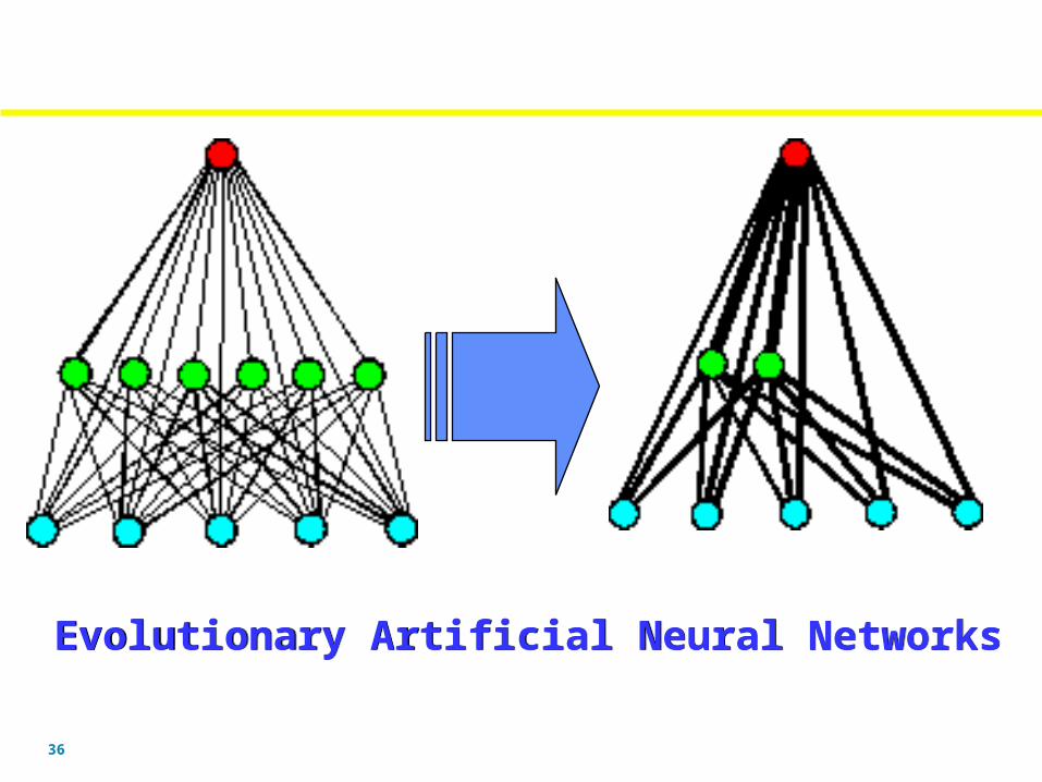
Evolutionary Artificial Neural NetworksEvolutionary Artificial Neural Networks

37
Evolutionary Neural Networks – Design StrategyEvolutionary Neural Networks – Design Strategy
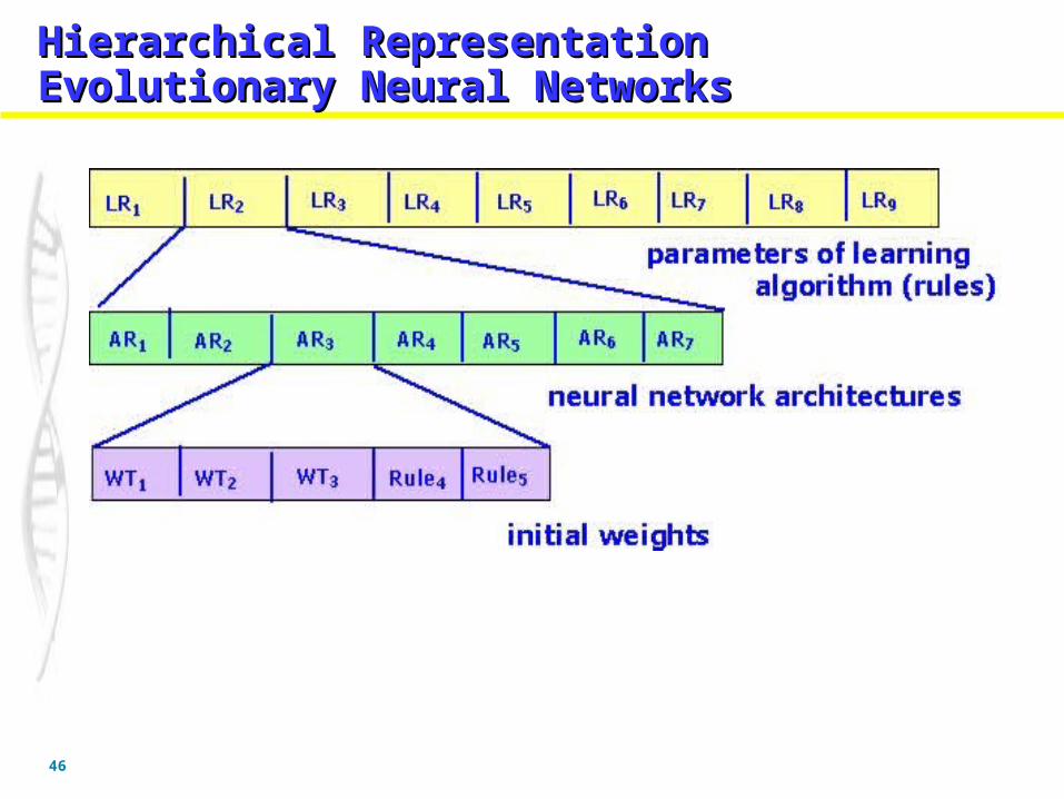
• Complete adaptation is achieved through three levels of evolution, i.e., the evolution of connection weights, architectures and learning rules (algorithms), which progress on different time scales.
38
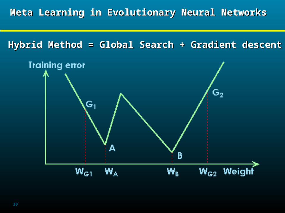
Meta Learning in Evolutionary Neural NetworksMeta Learning in Evolutionary Neural NetworksMeta Learning in Evolutionary Neural NetworksMeta Learning in Evolutionary Neural Networks
Hybrid Method = Global Search + Gradient descentHybrid Method = Global Search + Gradient descent
39
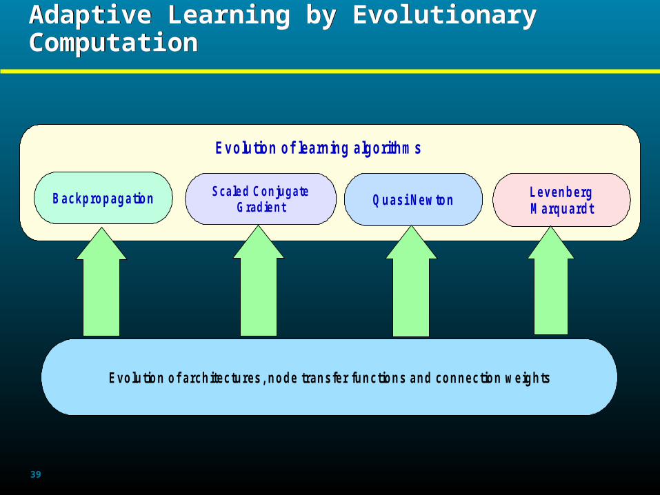
Adaptive Learning by Evolutionary ComputationAdaptive Learning by Evolutionary Computation
Backpropagation Scale d ConjugateGradie nt Quasi Newton Levenberg
M arquardt
Evolution of learning algorithms
Evolution of architectures, node transfer functions and connection weights
40
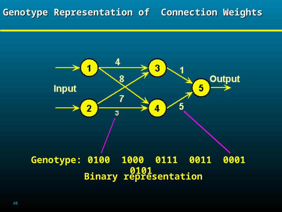
Genotype Representation of Connection WeightsGenotype Representation of Connection WeightsGenotype Representation of Connection WeightsGenotype Representation of Connection Weights
Genotype: 0100 1000 0111 0011 0001 0101
Binary representationBinary representation
41
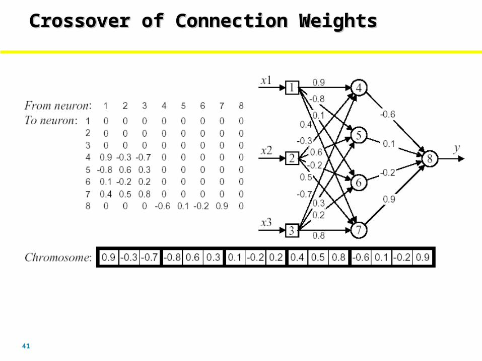
Crossover of Connection WeightsCrossover of Connection WeightsCrossover of Connection WeightsCrossover of Connection Weights

42
Crossover of Connection WeightsCrossover of Connection WeightsCrossover of Connection WeightsCrossover of Connection Weights
43
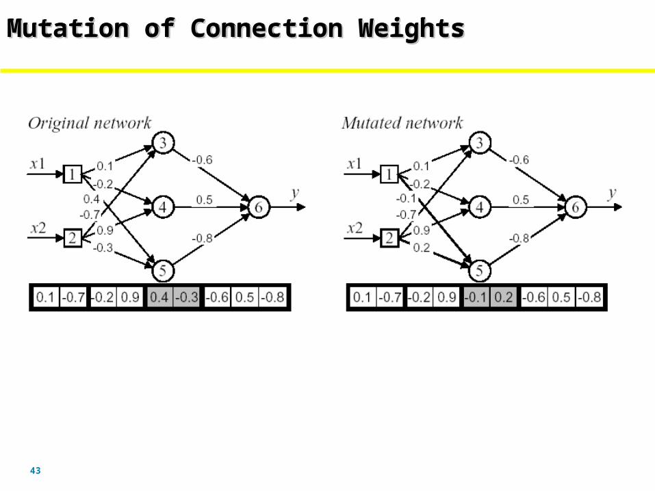
Mutation of Connection WeightsMutation of Connection WeightsMutation of Connection WeightsMutation of Connection Weights

44
Genotype Representation of ArchitecturesGenotype Representation of ArchitecturesGenotype Representation of ArchitecturesGenotype Representation of Architectures
45
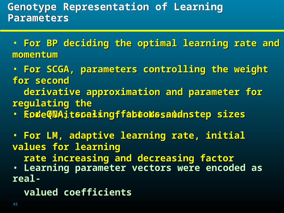
Genotype Representation of Learning ParametersGenotype Representation of Learning Parameters
• For BP deciding the optimal learning rate and momentumFor BP deciding the optimal learning rate and momentum
• Learning parameter vectors were encoded as real-Learning parameter vectors were encoded as real-
valued coefficientsvalued coefficients
• For SCGA, parameters controlling the weight for second For SCGA, parameters controlling the weight for second derivative approximation and parameter for regulating the derivative approximation and parameter for regulating the indefiniteness of the Hessian.indefiniteness of the Hessian.
• For QNA, scaling factors and step sizesFor QNA, scaling factors and step sizes
• For LM, adaptive learning rate, initial values for learning For LM, adaptive learning rate, initial values for learning rate increasing and decreasing factorrate increasing and decreasing factor
46
Hierarchical Representation Evolutionary Hierarchical Representation Evolutionary Neural NetworksNeural NetworksHierarchical Representation Evolutionary Hierarchical Representation Evolutionary Neural NetworksNeural Networks
47
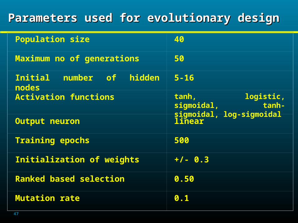
Parameters used for evolutionary designParameters used for evolutionary designParameters used for evolutionary designParameters used for evolutionary design
Population size 40
Maximum no of generations 50
Initial number of hidden nodes 5-16
Activation functions tanh, logistic, sigmoidal, tanh-sigmoidal, log-sigmoidal
Output neuron linear
Training epochs 500
Initialization of weights +/- 0.3
Ranked based selection 0.50
Mutation rate 0.1

48
EANN Convergence Using BP LearningEANN Convergence Using BP Learning
49
EANN Performance - Mackey Glass seriesEANN Performance - Mackey Glass series

50
EANN Performance - Gas Furnace SeriesEANN Performance - Gas Furnace Series
51
EANN Performance – Waste Water Flow SeriesEANN Performance – Waste Water Flow Series

52
Performance Evaluation among EANN and ANNPerformance Evaluation among EANN and ANN
Learning algorithm
EANN ANN
RMSE Hidden Layer Architecture
RMSE
BP 0.0077 7(T), 3(LS) 0.0437 24(TS)
SCG 0.0031 11(T) 0.0045 24(TS)
QNA 0.0027 6(T),4(TS) 0.0034 24(TS)
LM 0.0004 8(T),2(TS),1(LS)
0.0009 24(TS)
Mackey Glass seriesMackey Glass series
Hidden Layer Architecture
53
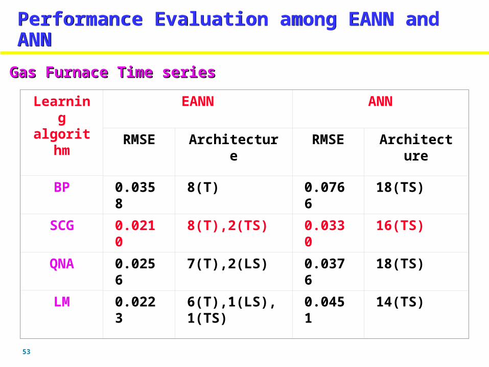
Performance Evaluation among EANN and ANNPerformance Evaluation among EANN and ANN
Learning algorithm
EANN ANN
RMSE Architecture RMSE Architecture
BP 0.0358 8(T) 0.0766 18(TS)
SCG 0.0210 8(T),2(TS) 0.0330 16(TS)
QNA 0.0256 7(T),2(LS) 0.0376 18(TS)
LM 0.0223 6(T),1(LS),1(TS)
0.0451 14(TS)
Gas Furnace Time seriesGas Furnace Time series
54
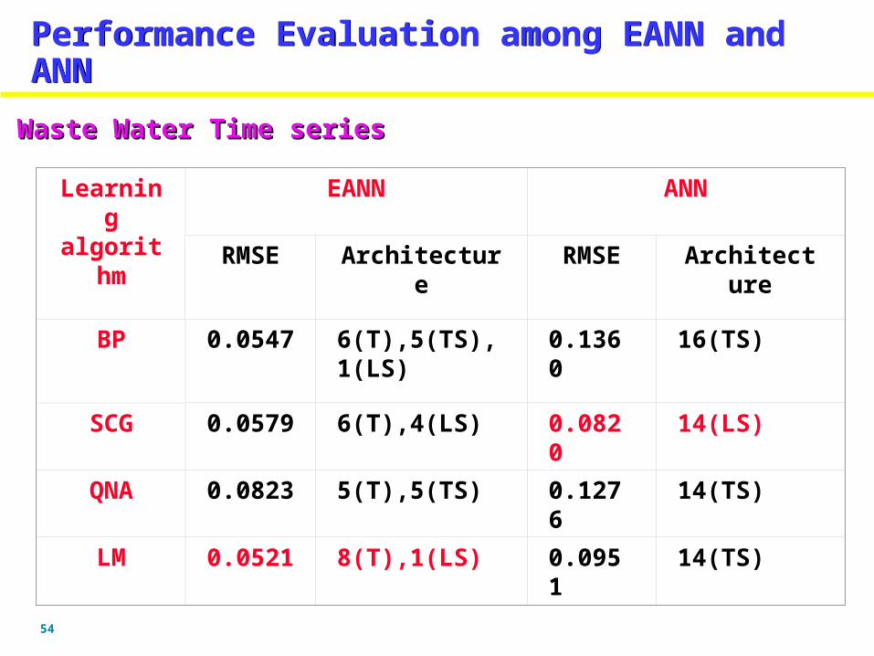
Performance Evaluation among EANN and ANNPerformance Evaluation among EANN and ANN
Waste Water Time seriesWaste Water Time series
Learning algorithm
EANN ANN
RMSE Architecture RMSE Architecture
BP 0.0547 6(T),5(TS),1(LS)
0.1360 16(TS)
SCG 0.0579 6(T),4(LS) 0.0820 14(LS)
QNA 0.0823 5(T),5(TS) 0.1276 14(TS)
LM 0.0521 8(T),1(LS) 0.0951 14(TS)

55
Efficiency of Evolutionary Neural NetsEfficiency of Evolutionary Neural Nets
• Designing the architecture and correct learning algorithm is a
tedious task for designing an optimal artificial neural network.
• For critical applications and H/W implementations optimal design
often becomes a necessity.
Disadvantages of EANNs
Computational complexity , Success depends on genotype
representation.
Empirical results show the efficiency of EANN procedure
• Average Number of hidden neurons reduced by more than 45%
• Average RMSE on test set down by 65%
Future works
• More learning algorithms, evaluation of full population information
(final generation).
56
Advantages of Neural NetworksAdvantages of Neural NetworksAdvantages of Neural NetworksAdvantages of Neural Networks
• Universal approximators Universal approximators
• Capturing associations or discovering
regularities within a set of patterns
• Can handle large no of variables and huge
volume of data
• Useful when conventional approaches can’t be
used to model relationships that are vaguely
understood
57
Evolutionary Fuzzy SystemsEvolutionary Fuzzy Systems

58
Fuzzy Expert SystemFuzzy Expert SystemA fuzzy expert system to forecast the reactive power (P) at time t+1 by knowing the load current (I) and voltage (V) at time t.
The experiment system consists of two stages:
Developing the fuzzy expert system and performance evaluation using the test data.
The model has two input variables (V and I) and one output variable (P).
Training and testing data sets were extracted randomly from the master dataset. 60% of data was used for training and remaining 40% for testing.
59
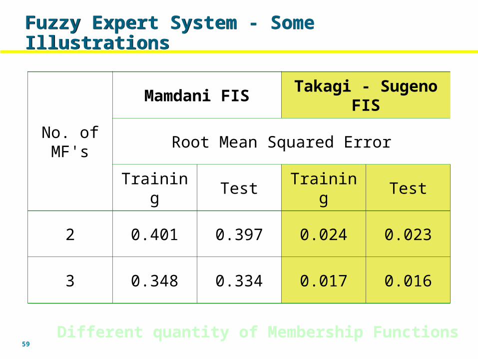
Fuzzy Expert System - Some IllustrationsFuzzy Expert System - Some Illustrations
No. of MF's
Mamdani FIS Takagi - Sugeno FIS
Root Mean Squared Error
Training Test Training Test
2 0.401 0.397 0.024 0.023
3 0.348 0.334 0.017 0.016
Different quantity of Membership Functions
60
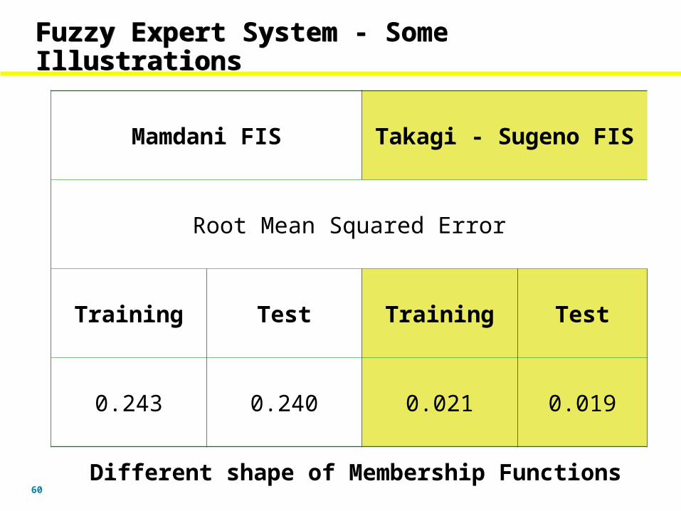
Mamdani FIS Takagi - Sugeno FIS
Root Mean Squared Error
Training Test Training Test
0.243 0.240 0.021 0.019
Different shape of Membership Functions
Fuzzy Expert System - Some Illustrations Fuzzy Expert System - Some Illustrations
61
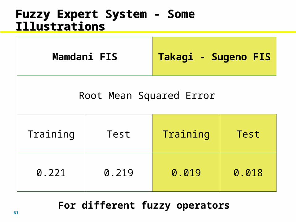
Mamdani FIS Takagi - Sugeno FIS
Root Mean Squared Error
Training Test Training Test
0.221 0.219 0.019 0.018
For different fuzzy operators
Fuzzy Expert System - Some IllustrationsFuzzy Expert System - Some Illustrations
62
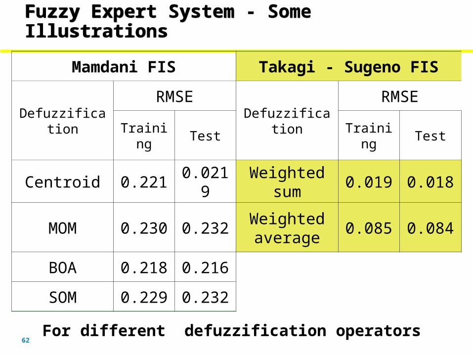
Mamdani FIS Takagi - Sugeno FIS
Defuzzification
RMSE
Defuzzification
RMSE
Training Test Training Test
Centroid 0.221 0.0219Weighted
sum0.019 0.018
MOM 0.230 0.232Weighted average
0.085 0.084
BOA 0.218 0.216
SOM 0.229 0.232
For different defuzzification operators
Fuzzy Expert System - Some IllustrationsFuzzy Expert System - Some Illustrations
63
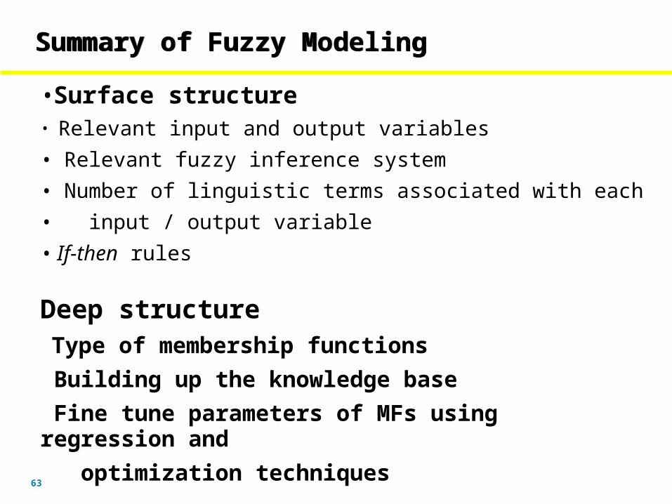
Summary of Fuzzy Modeling Summary of Fuzzy Modeling
•Surface structure• Relevant input and output variables
• Relevant fuzzy inference system
• Number of linguistic terms associated with each
• input / output variable
• If-then rules
Deep structure Type of membership functions
Building up the knowledge base
Fine tune parameters of MFs using regression and
optimization techniques
64
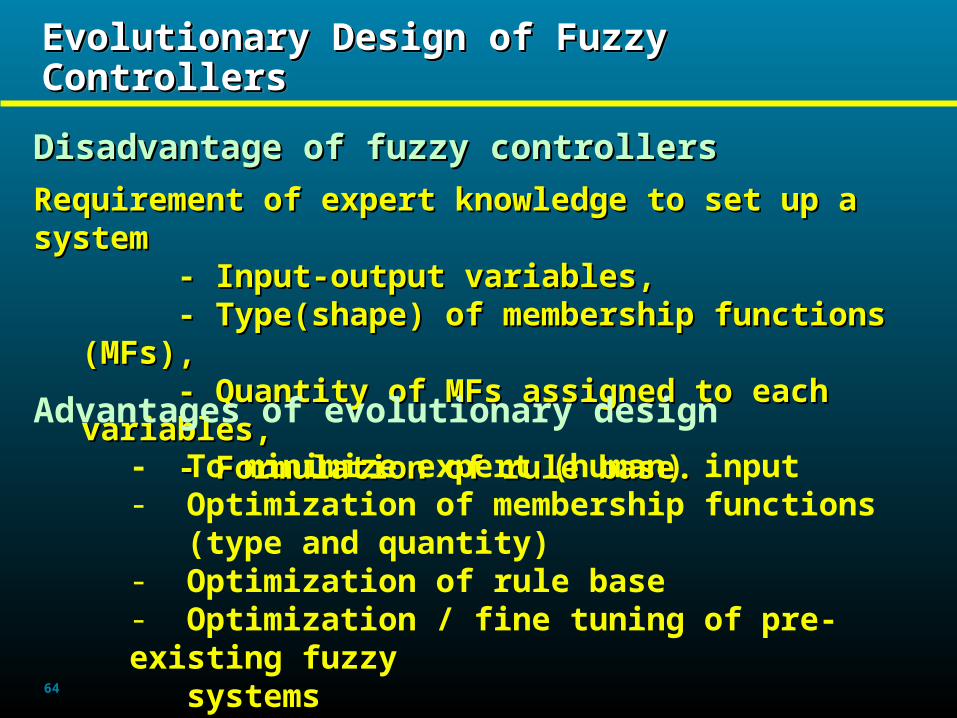
Evolutionary Design of Fuzzy ControllersEvolutionary Design of Fuzzy ControllersEvolutionary Design of Fuzzy ControllersEvolutionary Design of Fuzzy Controllers
Disadvantage of fuzzy controllersDisadvantage of fuzzy controllers
Requirement of expert knowledge to set up a Requirement of expert knowledge to set up a systemsystem
- Input-output variables, - Input-output variables, - Type(shape) of membership functions - Type(shape) of membership functions
(MFs),(MFs),- Quantity of MFs assigned to each - Quantity of MFs assigned to each
variables,variables,- Formulation of rule base.- Formulation of rule base.
Advantages of evolutionary design
- To minimize expert (human) input- Optimization of membership functions (type and quantity)- Optimization of rule base- Optimization / fine tuning of pre-existing fuzzy systems
65
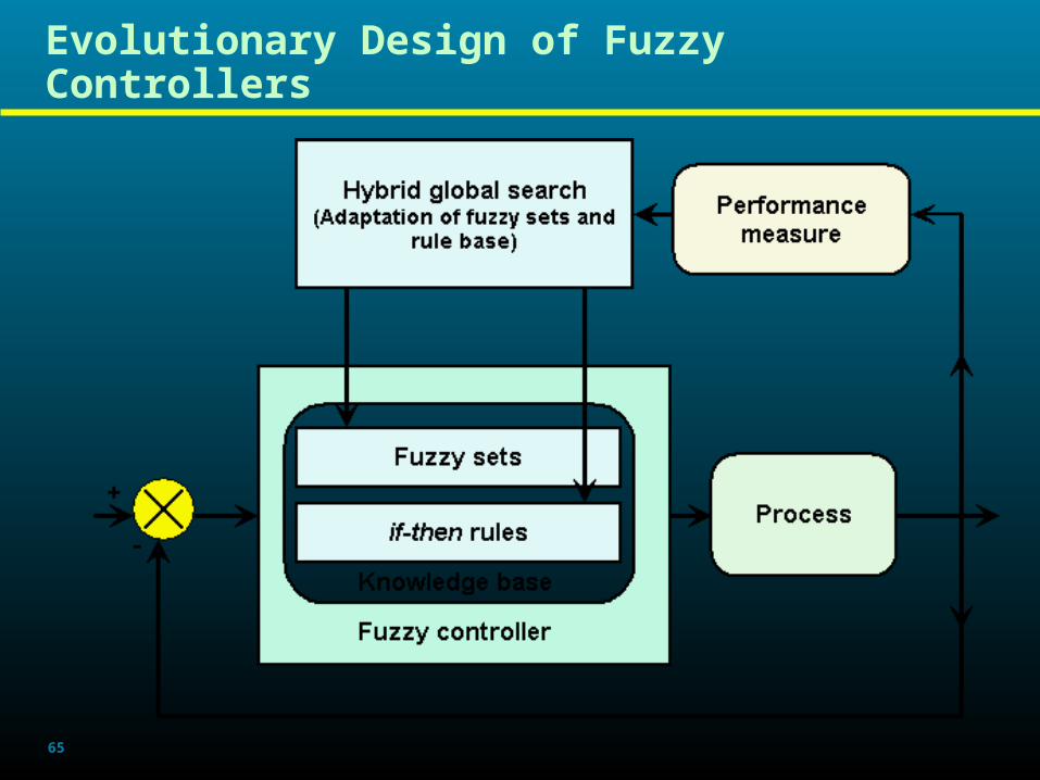
Evolutionary Design of Fuzzy Controllers
66
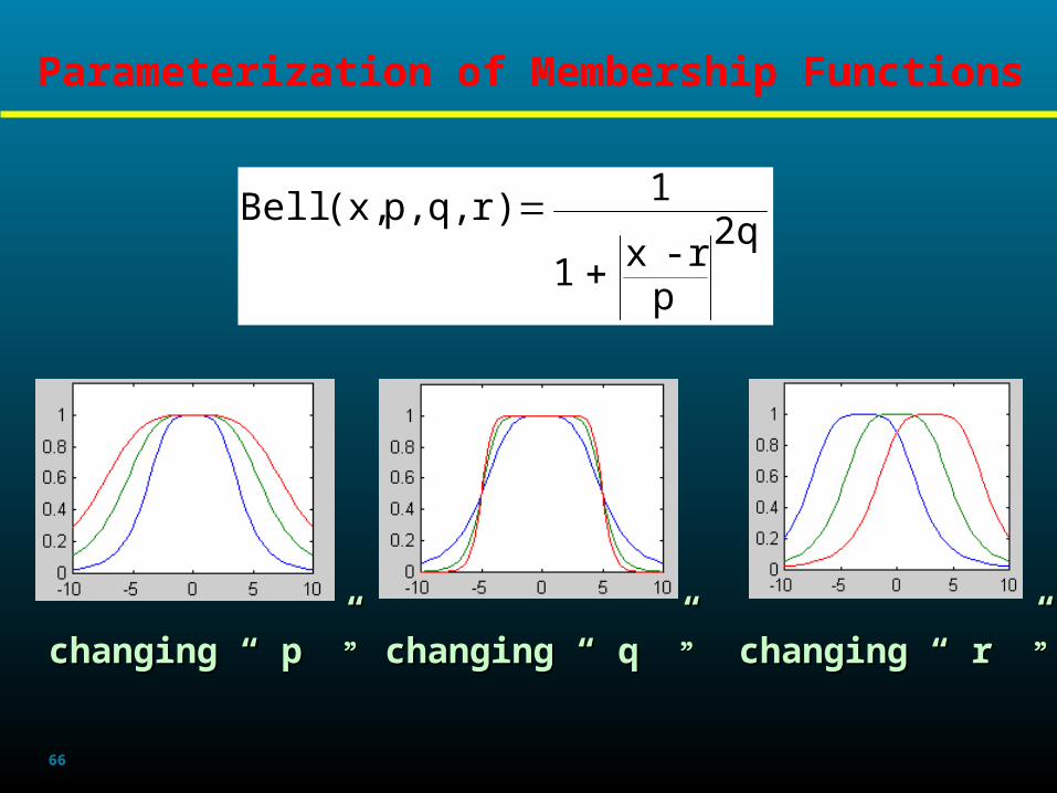
Parameterization of Membership Functions
2q
pr-x1
1r)q,p,(x,Bell
changing “ p ”changing “ p ””” changing “ q ”changing “ q ””” changing “ r ”changing “ r ”””
67
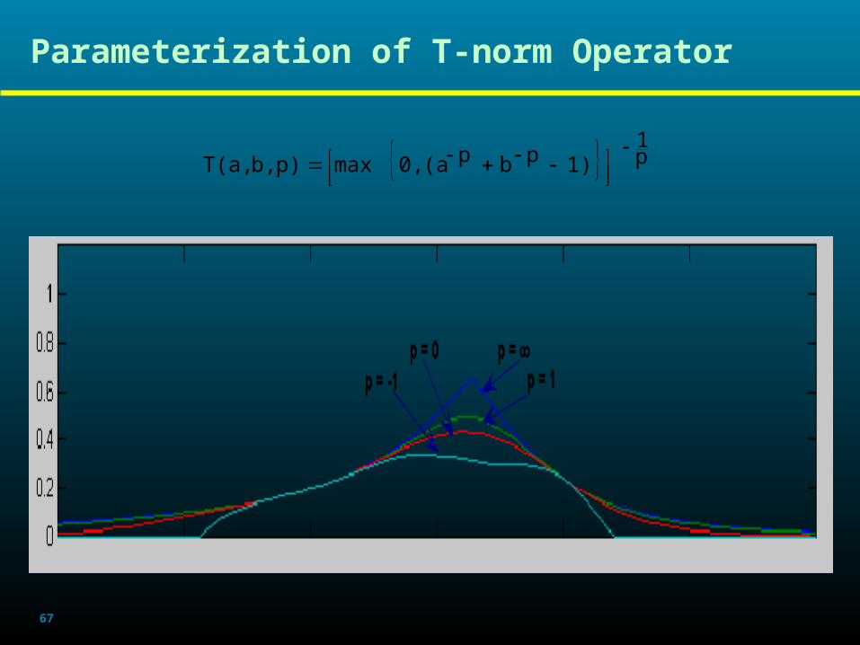
Parameterization of T-norm Operator
p1
1)pbp(a0,maxp)b,T(a,
68
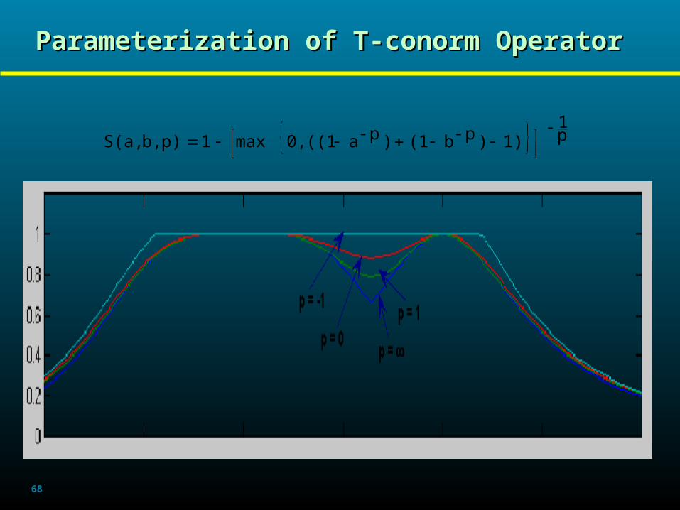
Parameterization of T-conorm OperatorParameterization of T-conorm Operator
p1
1))pb(1)pa((10,max1p)b,S(a,
69
Learning with Evolutionary Fuzzy SystemsLearning with Evolutionary Fuzzy Systems
•Evolutionary algorithms are not learning algorithms. They offer a powerful and domain independent search method for a variety of learning tasks.
•Three popular approaches in which evolutionary algorithms have been applied to the learning process of the fuzzy systems:
•- Michigan approach
- Pittsburgh approach
- Iterative rule learning
•Description of the above techniques follows …..
70
Michigan Approach
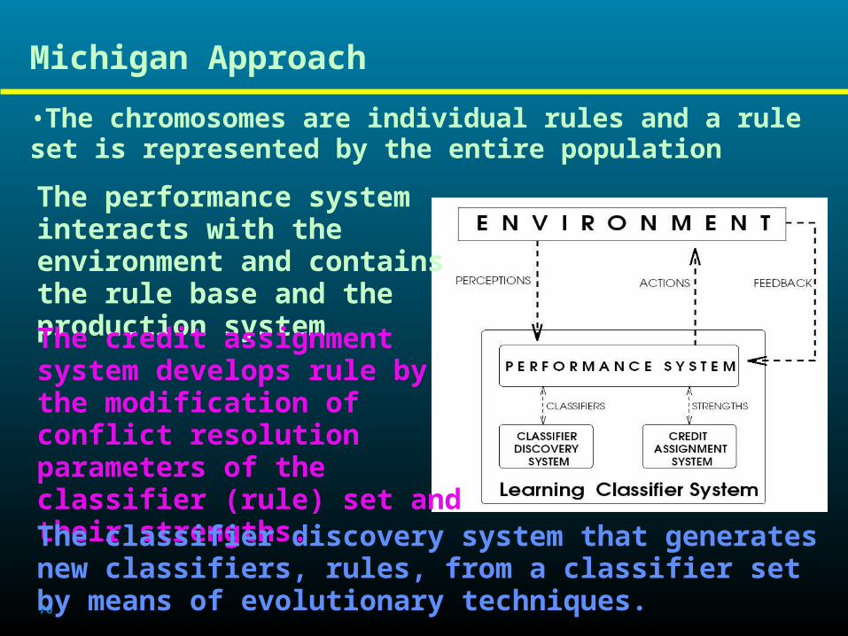
•The chromosomes are individual rules and a rule set is represented by the entire population
The performance system interacts with the environment and contains the rule base and the production systemThe credit assignment system develops rule by the modification of conflict resolution parameters of the classifier (rule) set and their strengths.The classifier discovery system that generates new classifiers, rules, from a classifier set by means of evolutionary techniques.
71
Pittsburgh Approach
• The chromosome encodes a whole rule base or • knowledge base.
• Crossover helps to provide new combination of rules• Mutation provides new rules
• Variable-length rule bases are used in some cases
with special genetic operators for dealing with these
variable-length and position independent genomes
• While Michigan approach might be useful for online-
learning Pittsburgh approach seem to be better suited
for batch-mode learning.
72
Iterative Rule Learning Approach
• The chromosome encodes individual rules like in • Michigan approach. Only the best individual is • considered to form part of the solution.
•The procedure….
1. Use a EA to obtain a rule for the system
2. Incorporate the rule into the final set of rules
3. Penalize this rule
4. If the set of rules obtained till now is adequate to be
a solution o the problem, the system ends up
returning the set of rules as the solution. Else return to
step 1.
73
Genotype Representation of Membership Genotype Representation of Membership FunctionsFunctions
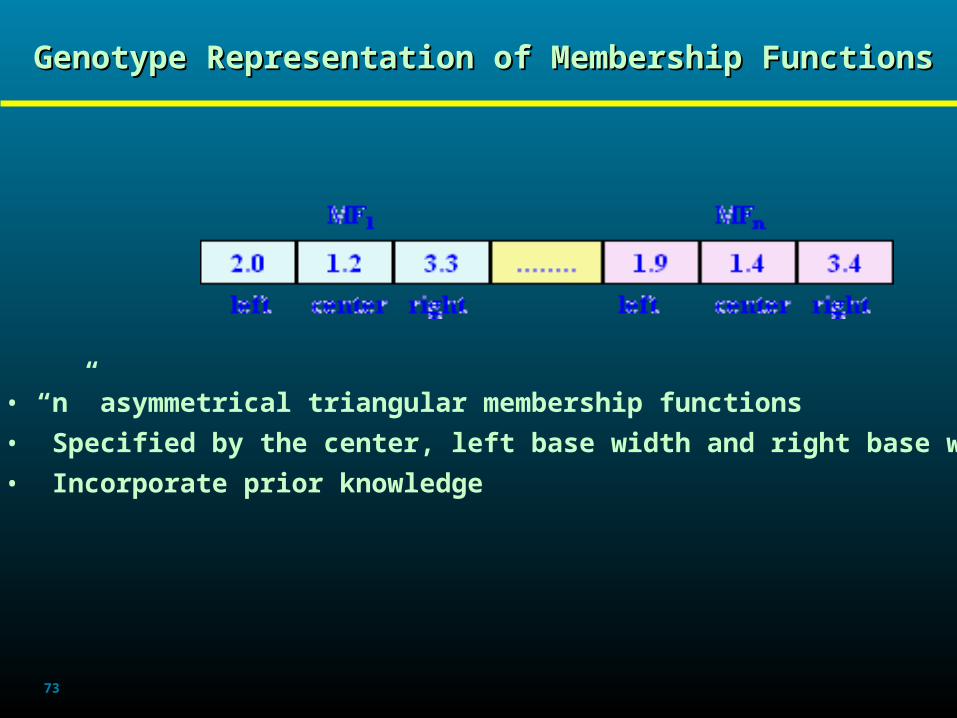
• “n” asymmetrical triangular membership functions
• Specified by the center, left base width and right base width
• Incorporate prior knowledge
74
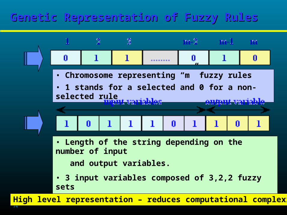
Genetic Representation of Fuzzy RulesGenetic Representation of Fuzzy Rules
• Chromosome representing “m” fuzzy rules
• 1 stands for a selected and 0 for a non-selected rule
• Length of the string depending on the number of input
and output variables.
• 3 input variables composed of 3,2,2 fuzzy sets
• 1 output variable composed of 3 fuzzy setsHigh level representation – reduces computational complexity
75
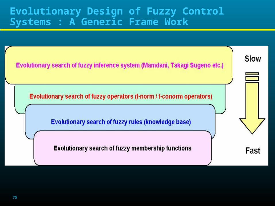
Evolutionary Design of Fuzzy Control Systems : A Generic Frame Work
76
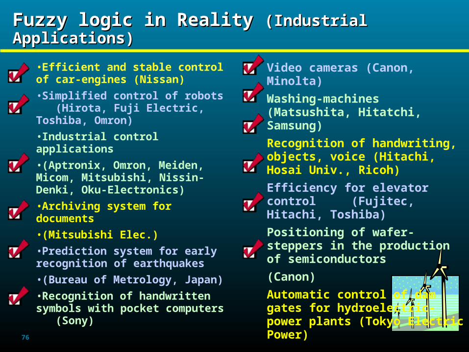
Fuzzy logic in Reality Fuzzy logic in Reality (Industrial Applications)(Industrial Applications)Fuzzy logic in Reality Fuzzy logic in Reality (Industrial Applications)(Industrial Applications)
•Efficient and stable control of car-engines (Nissan)
•Simplified control of robots (Hirota, Fuji Electric, Toshiba, Omron)
•Industrial control applications
•(Aptronix, Omron, Meiden, Micom, Mitsubishi, Nissin-Denki, Oku-Electronics)
•Archiving system for documents
•(Mitsubishi Elec.)
•Prediction system for early recognition of earthquakes
•(Bureau of Metrology, Japan)
•Recognition of handwritten symbols with pocket computers (Sony)
Video cameras (Canon, Minolta)
Washing-machines (Matsushita, Hitatchi, Samsung)
Recognition of handwriting, objects, voice (Hitachi, Hosai Univ., Ricoh)
Efficiency for elevator control (Fujitec, Hitachi, Toshiba)
Positioning of wafer-steppers in the production of semiconductors
(Canon)
Automatic control of dam gates for hydroelectric-power plants (Tokyo Electric Power)


![Evolving Synaptic Plasticity with an Evolutionary …...been suggested for such systems, including Artificial Ontogeny [8], Computational Embryogeny [9], Cellular Encoding [10,11],](https://img.pdfslide.net/doc/110x75/5f3f8ae8693e0a7d4e5ec431/evolving-synaptic-plasticity-with-an-evolutionary-been-suggested-for-such-systems.jpg)