Embed Size (px)
Citation preview

1
Introduction to Biostatistics (PUBHLTH 540) Estimating Parameters
• Which estimator is best? • Study possible samples, determine Expected values, bias,
variance, MSE– with replacement example– without replacement example (Exam 1)
• Estimate population mean– point estimator (sample mean)– interval estimator (95% central width)
• Central Limit theorem• Interval estimators based on a sample
– estimating the standard error– determining the multiplier (normal and t-distributions)

2
Sampling with replacement
• Program ejs09b540p19.sas– uses Arrays, Outputs, and Transpose– Select SRS w rep from N=5 with n=3 – Uniform random number generator
• Program ejs09b540p20.sas– Replaces sample size, pop size, and trials with
macro variables (gives flexibility)– Uses functions of arrays to get mean, var, min,
max– Select SRS w rep from N=5 with n=3

3
SRS without Replacement• Program ejs09b540p21.sas
– Process of selecting subjects without replacement
– Do loops, shifting indices etc.
• Program ejs09b540p22.sas– Implementable version with macro
variables
• Program ejs09b540p23.sas– Check that all sample sets have equal
probability– n=3 from N=3 with functions to get sets

4
Which Estimator of Population Median is Best?
• Program ejs09b540p24.sas– Add data from population, and link
response for sample subject sets– Evaluate sample median, mean,
(min+max)/2
• Program ejs09b540p25.sas– Summarize results of samples- using
expected value, variance, MSE of estimators
– Use PROC MEANS options for VARDEF=N, and MAXDEC=2
– Sample mean has smallest MSE– Is this always true?

5
Estimate Pop Median Age in Seasons Study Data
• Program ejs09b540p26.sas– use basev2.sas7bdat with “Age”– include histograms of distribution of
estimator over possible samples– best estimator is not the mean!- BEST
depends on the population…
• Program ejs09b540p27.sas– estimate Pop Mean using sample mean
from SRS w/o rep. of n=25– How does var of sample means relate to
the population variance?

6
Relating Population Variance to the Variance of the Sample Means
• Population Variance
• Variance of Sample Mean (without replacement:
• with T=10,000 trials…
2
var 11
N nX
N N n
22
1
1 N
ii
xN
273 25 57.37var 1 2.09
272 273 25X

7
Interval Estimate
• idea is to place an interval around an estimate to approximate the width of the estimators sampling distribution
• usually, the width is the central 95% of the estimators sampling distribution
• How wide is this?– measure width in terms of stderr of mean
2
var 11
N nSE X X
N N n
n

8
How good is Approximation?
• Program ejs09b540p28.sas– SRS w/o rep of n=5 to estimate Mean
LDL cholesterol from the Seasons study using the sample mean, 10 samples.
– determine the 2.5th percentile and 97.5th percentile of the distribution of sample means.
– Determine how many multiples of stderror of mean the percentiles are from the population mean

9
Example of 95% Width• Program ejs09b540p28.sas
• Change number of samples to 10000• Determine multiples for standard error
– Lower 2.5% multiplier is -1.85– Upper 97.5 multiplier is 2.02– Standard Deviation of sample means =
se(Mean)=15.94
• Program ejs09b540p30.sas– select srs w/o rep of n=5, estimate mean
• sample mean=166.7• Low= 166.7 -1.85(15.94)• High=166.7 + 2.02 (15.94)

10
Figure 1a. Histogram of tg for Population of N=291
Source: ejs09b540p31.sas 10/22/2009 by ejs
0 60 120 180 240 300 360 420 480 540 600 660 720 780 840 900 960 1020 1080 1140 1200 1260 1320 1380 1440 1500 1560 1620 1680
0
5
10
15
20
25
30
35
40
Pe
rce
nt
triglycerides:* tg
Example of Triglycerides- Seasons Study

11
Example of Triglycerides- Seasons Study
1.5
Take 10,000 SRS w/o replacement of size n=5 (program ejs09b540p31.sas)
Population:
Source Sim Sim Sim Sim
2 142 95.10 100.03 -0.93 2.55
5 144.1 62.07 63.26 -1.1 2.51
10 144.6 45.29 44.73 -1.19 2.95
20 144 30.81 31.63 -1.39 2.6
30 143.7 24.60 25.83 -1.47 2.49
50 143.6 18.10 20.01 -1.63 2.22
Source ejs09b540p31.sas
1
1 T
tt
Y YT
2
1
1
1
T
t tt
sd Y Y YT
n
n
Multiplier of for 2.5 %ile
tsd Y
Multiplier of for 97.5 %ile
tsd Y

12
Example of Triglycerides- Seasons Study
Figure 2. Histogram of sample means of n=10 for tg from Population of N=291
Source: ejs09b540p31.sas 10/22/2009 by ejs
0 20 40 60 80 100 120 140 160 180 200 220 240 260 280 300 320 340 360 380 400 420 440
0
5
10
15
20
25
30
35
40
Pe
rce
nt
mn_samp

13
Example of Triglycerides- Seasons Study
Figure 2. Histogram of sample means of n=20 for tg from Population of N=291
Source: ejs09b540p31.sas 10/22/2009 by ejs
0 20 40 60 80 100 120 140 160 180 200 220 240 260 280 300 320 340 360 380 400 420 440
0
5
10
15
20
25
30
35
40
Pe
rce
nt
mn_samp
14
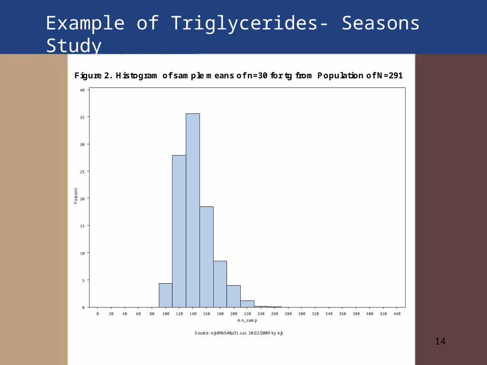
Example of Triglycerides- Seasons Study
Figure 2. Histogram of sample means of n=30 for tg from Population of N=291
Source: ejs09b540p31.sas 10/22/2009 by ejs
0 20 40 60 80 100 120 140 160 180 200 220 240 260 280 300 320 340 360 380 400 420 440
0
5
10
15
20
25
30
35
40
Pe
rce
nt
mn_samp

15
Example of Triglycerides- Seasons Study
Figure 2. Histogram of sample means of n=50 for tg from Population of N=291
Source: ejs09b540p31.sas 10/22/2009 by ejs
0 20 40 60 80 100 120 140 160 180 200 220 240 260 280 300 320 340 360 380 400 420 440
0
10
20
30
40
50
Pe
rce
nt
mn_samp

16
Example of Triglycerides- Seasons Study
Figure 2. Histogram of sample means of n=50 for tg from Population of N=291
Source: ejs09b540p31.sas 10/22/2009 by ejs
0 20 40 60 80 100 120 140 160 180 200 220 240 260 280 300 320 340 360 380 400 420 440
0
10
20
30
40
50
Pe
rce
nt
mn_samp

17
Example of Triglycerides- Seasons Study
Sa
mp
le
1
21
41
61
81
101
121
141
161
181
201
221
241
261
281
tg 95% Interval Estimate
0 20 40 60 80 100 120 140 160 180 200 220 240 260 280 300 320 340 360 380 400 420 440
Figure 1. Illustration of Point and 95% Interval Estimate for n=50 for tg
Source: ejs09b540p30.sas 10/20/2009 by ejs
id 1

18
Conclusions
• With larger sample size, distribution of sample means is more bell shaped (i.e. ‘normal’) (Central Limit Theorem)
• Central 95% of distribution is around + or - 2 standard errors from true population mean
• In practice we don’t know the SE• In practice we don’t know the multiplier• Solution: Estimate SE from sample• Solution: Approximate multipler
assuming a distribution (Normal if known or t-distribution if not known)

19
Normal Distribution
• With larger sample sizes, the distribution of SRS means is normal:
2,y yY N 2
2y n
• Standard Normal Distribution
0,1y
YZ N

20
Transforming a Random Variable
• Standardization is an example of transforming a random variable.
• Suppose we have a random variable:
Y
• What is the expected value and variance of X=a+bY?
yE Y 2var yY
y
x
E X E a bY
a bE Y
a b

21
Transforming a Random Variable
• Variance of X=a+bY?
2
2
2
22
2 2
var var
y
y
y
y
X a bY
E X E X
E a bY a b
E b Y
b E Y
b

22
Transforming a Random Variable
• Application for Standardizing
1 1yy
y y y
YZ Y
1y
y
a
1
y
b
Z a bY
1 1
0y yy y
E Z a bE Y
2
2
2
var var
11y
y
Z b Y

23
Conclusions- Practical
• Assume Central Limit Theorem holds (usually if n>30)
• Use multiplier based on centered distribution of standard normal (if
is known)
• see Table A3 in Text– central 60% -0.84 to +0.84
– central 80% -1.28 to 1.28
– central 90% -1.64 to 1.64
– central 95% -1.96 to 1.96
– central 99% -2.56 to 2.56
20, 1Z N

24
Conclusions- Practical
• In practice we don’t know
• Estimate using
• Use a t-distribution with (n-1) degrees of freedom for multiplies (see table A4 in text).– assumes underlying normal
distribution and srs
x
var xX SE Xn
22
1
1
1
n
ii
S X Xn

25
Conclusions- Practical
• t-distribution examples for 95% interval estimator (Confidence interval):– n=2 df=1 -4.3 to 4.3– n=5 df=4 -2.776 to 2.776– n=10 df=9 -2.262 to 2.262– n=20 df=19 -2.093 to 2.093– n=30 df=29 -2.045 to 2.045– n=50 df=49 -2.009 to 2.009– n=120df=119 -1.98 to 1.98– n=500df=499 -1.96 to 1.96