Embed Size (px)
Citation preview

1
Joint Channel and Doppler Offset Estimation in
Dynamic Cooperative Relay NetworksIdo Nevat1, Gareth W. Peters 2,3, Arnaud Doucet 4 and Jinhong Yuan5
1 Wireless & Networking Tech. Lab, CSIRO, Sydney, Australia.2 Department of Statistical Science, University College London, London, UK.
3 CSIRO Mathematical and Information Sciences, Sydney, Australia.4 Department of Statistics, Oxford, UK.
5 School of Electrical Engineering,University of NSW, Sydney, Australia.
Abstract
We propose new algorithms to perform joint channel and Doppler offset estimation in dynamic
cooperative wireless relay networks. We first formulate the problem as a Bayesian non-linear state
space model, then develop two algorithms that are based on different sampling methodologies to jointly
estimate the dynamic channels and static Doppler offsets. The first is based on a MCMC-within-Gibbs
sampling methodology and the second is obtained via a novel development of a Particle Adaptive
Marginal Metropolis-Hastings method. We show that the Particle Adaptive Marginal Metropolis-Hastings
algorithm requires only a fraction of the computational complexity of the MCMC-within-Gibbs sampler.
In addition, we develop a version of the recursive marginal Cramer-Rao lower bound on the path space
which involves marginalistion of the static parameters. Simulation results demonstrate that the proposed
algorithm performs close to the Marginal Cramer-Rao Lower Bound.
Index Terms
Channel Estimation, Doppler Offset Estimation, Cooperative Relay Networks, Particle filter, MCMC.
I. INTRODUCTION
The relay channel, first introduced by van der Meulen [1], has recently received considerable attention
due to its potential in wireless applications. Relaying techniques have the potential to provide spatial
diversity, improve energy efficiency, and reduce the interference level of wireless channels, see [2], [3].
This work was presented in part at the 2011 IEEE VTC Conference in San Francisco, USA.
November 15, 2012 DRAFT
2
In order to utilise the relay channel, an accurate channel state information (CSI) is required at the
destination. When the communicating terminals are mobile, channels form a cascade of mobile-to-mobile
channels, and can change rapidly with time. Therefore, a dynamic time-varying channel model is required.
However, most current works concentrate on performing relay-based channel estimation (and assuming
no Doppler offset is present) in a static environment, where the channels are assumed to be block fading:
in [4], the authors designed two linear estimators, that is the Least Squares (LS) and Linear Minimum
Mean Squared Error (LMMSE) for Amplify and Forward (AF) based relay networks; in [5], an algorithm
for LMMSE channel estimation in OFDM based relay systems was derived; and in [6], a training based
LMMSE channel estimator for time division multiplex AF relay networks was proposed. A non-linear
state-space model was developed in [7] to perform a sub-optimal (linear) estimation (via Kalman filter)
under the assumption that the model parameters are known. The authors also reported that the relay
speed has a significant impact on the BER performance, and therefore it is important to estimate those
parameters accurately in cases where the Doppler offset is a-priori unknown.
The problem of joint channel tracking and Doppler offset estimation is of practical importance in
wireless communications [8], [9] [10], where in many networks the relays may be mobile. In these cases,
high user mobility leads to large and time varying Doppler frequencies at the destination. In relay wireless
links this problem has not been addressed yet and it involves jointly estimating the Doppler offset for
each link in the relay system, which we refer to as static parameters, and the channel tracking problem
in non-linear state-space model.
To solve this problem, we develop an efficient framework to perform Bayesian inference with respect
to filtering and parameter estimation in the resulting high-dimensional space. This involves development
of advanced Monte Carlo techniques which combine the strength of non-linear filtering frameworks,
such as Sequential Monte Carlo (SMC), with adaptive versions of Markov chain Monte Carlo (MCMC)
techniques [11].
In particular, we make the following contributions:
1) We propose a statistical model to address the inference problem of channel tracking and Doppler
offset estimation in relay networks, such that all quantities are estimated at the destination.
2) We develop two novel algorithms for joint channel tracking and Doppler estimation which are
based on the following methodologies:
∙ We develop a Rao-Blackwellised adaptive Particle MCMC (PMCMC) algorithm. The adaptive
MCMC algorithm we design provides an improved mixing rate, thus making the algorithm
November 15, 2012 DRAFT

3
more efficient (presented in Section V).
∙ We design a Gibbs sampler by splitting the high dimensional posterior distribution into sub-
blocks of parameters and then running a blockwise MCMC-within-Gibbs sampling framework
(presented in Section IV).
3) We perform complexity analisys and show that the PMCMC algorithm is much more efficient
and requires only a fraction of the computational complexity of the Gibbs sampler for the same
estimation accuracy.
4) We derive the marginal Cramer-Rao Lower Bound (CRLB) for the dynamic state-space model and
demonstrate that the proposed algorithm performs close to the bound.
Notation: random variables are denoted by upper case letters and their realizations by lower case letters;
bold face to denote vectors and non-bold for scalars; super script will be used to refer to the index for
a particular relay in the network; sub-script will denote discrete time, where ℎ1:T denotes ℎ1, . . . , ℎT ;
and in the sampling methodology combining MCMC and particle filtering we use the following notation
[⋅](j, i) to denote the j-th state of the Markov chain for the i-th particle in the particle filter. In addition,
we denote the proposed Markov chain state by [⋅]∗(j, i), and � (⋅) denotes the delta of Dirac.
II. SYSTEM DESCRIPTION
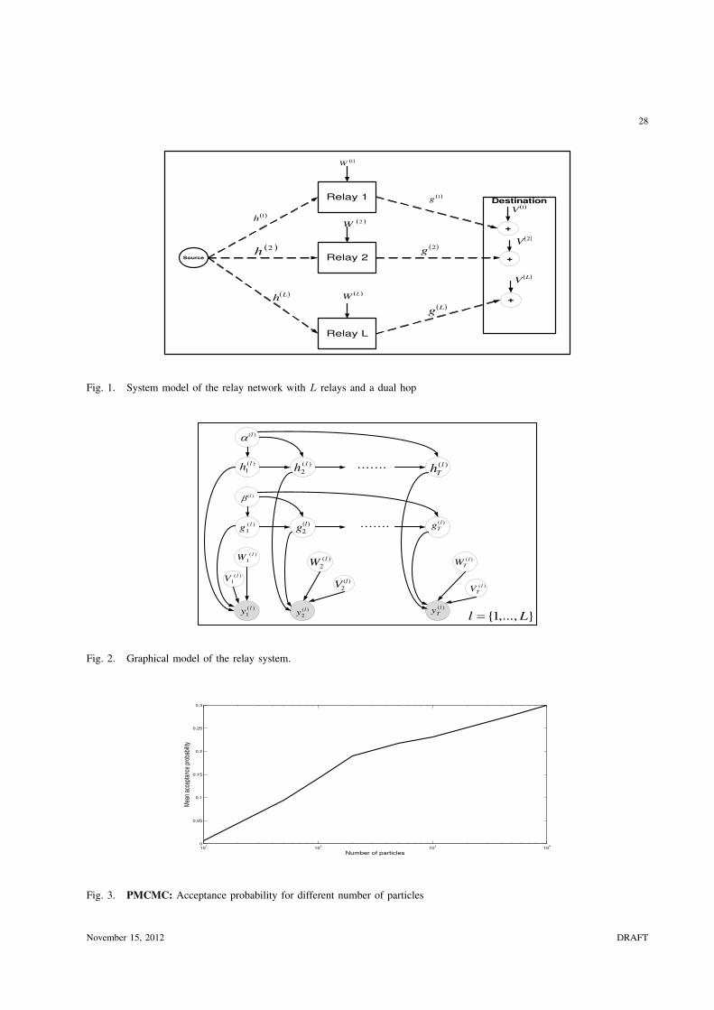
We consider the case where one mobile station is transmitting to a Base Station (BS) via L relays,
which may be mobile or stationary, see Fig. 1. We consider frequency-flat fading channels, and the
extension to multi-path channels is straight forward, for example via the use of OFDM modulation.
A. Statistical Model of Relay Network
i. Assume a wireless relay network with one mobile source node, transmitting symbols in frames of
length T to a Base Station (BS) via L mobile or stationary relays.
ii. We consider a half duplex transmission model in which the data for a given frame are transmitted
via a two step procedure. In the first step, the source node broadcasts a frame to all the relay
nodes. In the second step, the relay nodes transmit the processed frame, termed the relay signals,
to the destination node in orthogonal fashion, i.e. non-interfering channels via time division or
frequency devision multiplex, see for example [12], [13].
vi. The time-varying channels are parametrized under a Gauss-Markov model [14], [15]. The l-th
relay channel is modeled as a two stage latent stochastic process, in which at time n we denote
November 15, 2012 DRAFT

4
the realization of the two channel stages by ℎ(l)n and g
(l)n .
H(l)n = �(l)H
(l)n−1 +
√1−
(�(l))2Υ(l)
n
G(l)n = �(l)G
(l)n−1 +
√1−
(�(l))2Ω(l)n ,
(1)
where Υ(l)n ∼ CN (0, 1), Ω(l)
n ∼ CN (0, 1).
vii. The velocities of both the user and the relays are assumed constant over a frame and follow a
uniform distribution V(l)M→R ∼ U [0, vmax] and V
(l)R→D ∼ U [0, vmax], respectively, where vmax is a
practical upper bound.
viii. The channel coefficients �(l) and �(l) are modelled according to Jakes model as [16]
�(l) = J0
(2�
V(l)M→Rfc
cTs
)= J0
(2�F
(l)M→RTs
),
�(l) = J0
(2�
V(l)M→Rfc
cTs
)J0
(2�
V(l)R→Dfcc
Ts
)= J0
(2�F
(l)M→RTs
)J0
(2�F
(l)R→DTs
),
(2)
where J0 is the zeroth-order Bessel function of the first kind, fc is the carrier frequency, c is the
speed of light and Ts is the symbol duration [17], [18].
viii. The received signal at the l-th relay is a random variable given by
R(l)n = snH
(l)n +W (l)
n , l ∈ {1, . . . , L} , (3)
where at time n, H(l)n is the channel coefficient between the transmitter and the l-th relay, sn is
the transmitted pilot symbol and W(l)n is the noise realization associated with the relay receiver.
ix. The received signals at the destination is a random variable given by
Y (l)n = f (l)
(R(l)
n , n)G(l)
n + V (l)n , l ∈ {1, . . . , L} , (4)
where at time n, G(l)n is the channel coefficient between the l-th relay and the receiver. Generically,
the model we develop is general enough to allow for many different possible relay functions,
generally any mapping of the form f (l)(R(l), n
): ℝ 7→ ℝ, for any continous d-differentiable
functions f (l)(R(l), n
)∈ ℂd[ℝ] on the real line. As an example consider a relay function given by
the popular Amplify-and-Forward with constant gain [4], [6], with function
f (l)(R(l), n
)=
√√√⎷1
�2ℎ + �2
g +�2v
E[∣sn∣2]
(5)
where E
[∣sn∣2
]is the average symbols power.
November 15, 2012 DRAFT

5
x. All received signals are corrupted by i.i.d. zero-mean additive white complex Gaussian noise
(AWGN). At the l-th relay at the n-th transmitted symbol is denoted by W(l)n ∼ CN
(0, �2
w
).
Then at the receiver this is denoted by V(l)n ∼ CN
(0, �2
v
).
Based on the aforementioned assumptions, the following state-space model is presented by the graphical
model structure in Fig. 2, and is expressed as⎧⎨⎩
H(l)n = �(l)H
(l)n−1 +
√1−
(�(l))2Υ
(l)n , (State equation I)
G(l)n = �(l)G
(l)n−1 +
√1−
(�(l))2Ω(l)n , (State equation II)
Y(l)n = f (l)
(snH
(l)n +W
(l)n
)G
(l)n + V
(l)n (Observation equation) .
(6)
B. Channel and Doppler Offset estimation formulation
In order to formulate the problem, the distribution of transformed random variables J0
(2�F
(l)M→RTs
)
and J0
(2�F
(l)R→DTs
)need to be derived. To this end we recall that we used a uniform prior distribution
for the velocities of both mobile and relay terminals (point vii. of Section II-A). To accommodate for a
wide range of velocities, carrier frequencies and symbol rates, we set vmax = c�fcTs
.
Next, in the following Lemma we present the distribution functions of J0(2�F
(l)M→RTs
)and J0
(2�F
(l)R→DTs
).
Lemma 1: Under a uniform prior distribution of the mobile velocity, V ∼ U [0, vmax], its Doppler
offset follows a Beta distribution as follows:
J0
(2�
V fcc
Ts
)∼ Beta (1, 1/2) . (7)
Proof: We expend J0
(2� V fc
cTs
)via Taylor Series expansion around 0:
J0
(2�V fcTs
c
)=
∞∑
m=0
(−1)m
m!Γ (m+ 1)
(1
2
2�V fcTs
c
)2m
≈K∑
m=0
(−1)m
m!Γ (m+ 1)
(�V fcTs
c
)2m
≈︸︷︷︸K=1
1
Γ (1)− 1
Γ (2)
(�V fcTs
c
)2
= 1−(�V fcTs
c
)2
.
(8)
Next, we note that(�V fcTs
c
)∼ U [0, 1], and therefore, by utilising the power function distribution, we
obtain that(�V fcTs
c
)2∼ Beta (1/2, 1). Then, by using the mirror-image symmetry of the Beta distribution,
we obtain that(1−
(�V fcTs
c
)2)∼ Beta (1, 1/2).
November 15, 2012 DRAFT

6
Next, the posterior distribution can be expressed as:
p (�,�,g1:T ,h1:T ∣y1:T )
∝ p (y1:T ∣�,�,g1:T ,h1:T ) p (g1:T ,h1:T ∣�,�) p (�,�)
=
L∏
l=1
[T∏
n=1
∫p(y(l)n ∣�(l), �(l), g(l)n , ℎ(l)n , w(l)
n
)p(w(l)n
)dw(l)
n p(ℎ(l)n ∣ℎ(l)n−1
)p(g(l)n ∣g(l)n−1
)]
×L∏
l=1
p(g(l)1
)p(ℎ(l)1
)p(�(l))p(�(l))
=
L∏
l=1
⎡⎢⎣
T∏
n=1
1√2��2
v
∫exp
⎧⎨⎩−
∣∣∣y(l)n − f(snℎ
(l)n + w
(l)n
)g(l)n
∣∣∣2
2�2v
⎫⎬⎭
1√2��2
w
exp
⎧⎨⎩−
∣∣∣w(l)n
∣∣∣2
2�2w
⎫⎬⎭
dw(l)n
× 1√2�(1−
(�(l))2)
exp
⎧⎨⎩−
∣∣∣g(l)n − �(l)g(l)n−1
∣∣∣2
2(1−
(�(l))2)
⎫⎬⎭
1√2�(1−
(�(l))2)
exp
⎧⎨⎩−
∣∣∣ℎ(l)n − �(l)ℎ(l)n−1
∣∣∣2
2(1−
(�(l))2)
⎫⎬⎭
⎤⎥⎥⎦
× 1√2�
L∏
l=1
exp
{−1
2
∣∣∣g(l)1
∣∣∣2}
1√2�
L∏
l=1
exp
{−1
2
∣∣∣ℎ(l)1∣∣∣2}
×L∏
l=1
1
B (a, b)
(�(l))a−1 (
1− �(l))b−1
L∏
l=1
1
B (c, d)
(�(l))c−1 (
1− �(l))d−1
(9)
where �(1:L), �(1:L), g(1:L)1:T , ℎ
(1:L)1:T , y
(l:L)1:T ≜ �,�,g1:T ,h1:T ,y1:T .
Next we define the quantities of interest. Based on the marginal posterior in (9) we have:
MAP estimation(�MAP, �MAP, hMAP
1:T , gMAP1:T
)= argmax
�,�,g1:T ,h1:T
p (�,�,g1:T ,h1:T ∣y1:T ) . (10)
MMSE estimation(�MMSE, �MMSE, hMMSE
1:T , gMMSE1:T
)=
∫. . .
∫p (�,�,g1:T ,h1:T ∣y1:T ) � � g1:T h1:T d� d� dh1:T dg1:T .
(11)
Since the posterior model in (9) is very high dimensional with L(3T+2) parameters and highly nonlinear,
solving (10-11) requires advanced computational tools that will be the scope of the proposed algorithms.
Corollary 1: The posterior distribution in (9) factorises according to the following independence
structure
p (�,�,g1:T ,h1:T ∣y1:T ) =
L∏
l=1
p(�(l), �(l), g
(l)1:T , ℎ
(l)1:T ∣y
(l)1:T
), (12)
November 15, 2012 DRAFT

7
with respect to the number of parallel relay transmission paths.
Corollary 1 enables us to exploit the structure of the model in the design of the estimation framework.
In particular, the problem admits a block factorisation structure in which the particle filters per block may
be run independently. Thus, we are able to estimate the proposal distribution for the channels trajectories,
via parallel independent particle filters. Therefore, the variance of the incremental important weights used
in the estimation of the proposal can be reduced leading to an increased PMCMC acceptance probability.
Therefore, under the model and estimation procedure proposed, increasing the number of relays
will not degrade the solution.
C. The need for augmented Bayesian posterior
In order to perform inference, the likelihood function in (9), p(y(l)n ∣�(l), �(l), g
(l)n , ℎ
(l)n
), needs to be
evaluated. To achieve that we write the marginal distribution at the l-th relay as
pR
(l)n
(r∣sn, g(l)n , ℎ(l)n
)= p
(snℎ
(l)n + w(l)
n ∣sn, ℎ(l)n , g(l)n
)= CN
(snℎ
(l)n , �2
w
).
Then, finding the distribution of the random variable after the relay function is applied i.e. the distribution
of f(r(l)n
)≜ f
(r(l)n
)G
(l)n given sn, ℎ
(l)n , g
(l)n , involves the following change of variable formula
p(f(r(l)n
)∣sn, ℎ(l)n , g(l)n
)= p
R(l)n
((f (l))−1
(r(l)n
)∣sn, ℎ(l)n , g(l)n
) ∣∣∣∣∣∂f (l)
∂r(l)n
∣∣∣∣∣
−1
,
which can not always be written down analytically for an arbitrary relay function. The second complication
is that even if f(r(l)n
)is known, one must then solve the following convolution to obtain the likelihood:
p(y(l)n ∣sn, g(l)n , ℎ(l)n
)= p
(f(r(l)n
)∣sn, g(l)n , ℎ(l)n
)⊗ p
V(l)n
=
∫ ∞
−∞p(f(z∣sn, g(l)n , ℎ(l)n
))pV
(l)n
(y(l)n − z
)dz,
where ⊗ denotes the convolution operation. Typically this will be intractable to evaluate pointwise.
To circumvent this difficulty we utilise an augmented Bayesian posterior p (�,�,g1:T ,h1:T ,w1:T ∣y1:T ),
containing auxiliary variables W1:T which we marginalise out numerically in our sampling algorithm to
obtain the posterior corresponding to (9).
Under the augmented model, the likelihood function can now be expressed as
p(y(l)n ∣sn, g(l)n , ℎ(l)n , w(l)
n
)∼ CN
(f (l)
(snℎ
(l)n + w(l)
n
)g(l)n , �2
v
).
November 15, 2012 DRAFT

8
III. OVERVIEW OF MCMC METHODS
We now present a short overview of Markov Chain Monte Carlo (MCMC) methods that will be used
in the development of the two algorithms in Sections IV-V. MCMC is a class of Monte Carlo methods
for obtaining a sequence of random samples from a probability distribution for which direct sampling is
difficult. MCMC methods generate samples by running a reversible chain whose equilibrium distribution
is the desired target distribution [11]. An aperiodic and irreducible Markov chain has the property of
converging to a unique stationary distribution, �(x∣y), which does not depend on the initial sample. After
convergence, a MCMC method produces samples from the target distribution, �(x∣y), so that :
�(x∣y) = 1
J
J∑
j=1
� (x− x (j)) , (13)
where J is the number of samples generated. The most popular MCMC algorithm is based on Metropolis-
Hastings (MH) method. It uses a Markov transition kernel (proposal density), q(x∗;x (j − 1)), which
depends on the current state x (j − 1), to generate a new proposed sample x∗ and then accepts it
probabilistically via a rejection step. The generic MH algorithm is described by the following steps:
Algorithm 1 Generic Metropolis-Hastings MCMC Algorithm
1: Initialise x (1) to an arbitrary starting point.
2: Repeat steps (3− 6) for j = 2, . . . , J
3: Sample x∗ ∼ q (x∗;x (j − 1)) via a proposal density.
4: Compute the acceptance probability: A (x∗,x (j − 1)) = min{1, p(x∗∣y)
p(x(j−1)∣y) ×q(x(j−1);x∗)q(x∗;x(j−1))
}.
5: Generate a uniform random variable u ∼ U [0, 1] .
6: If u ≤ A (x∗,x (j − 1)) then x (j) = x∗ else x (j) = x (j − 1) end if.
The accuracy of the estimate in (10-11) depends on the choice of the Markov transition kernel
q(x∗;x (j − 1)). Choosing an appropriate proposal is particularly challenging in high dimensions and
when strong posterior correlation is present, as in our case, see (9).
IV. ALGORITHM I: JOINT CHANNEL AND DOPPLER ESTIMATION VIA MCMC-WITHIN-GIBBS
We develop a novel algorithm to estimate the MAP and MMSE estimates in (10-11) via a Gibbs
sampler framework [19]. The Gibbs sampler we develop involves splitting the high dimensional posterior
distribution into subblocks of parameters and then running a blockwise MCMC-within-Gibbs sampling
November 15, 2012 DRAFT

9
framework. In the proposed Gibbs sampling framework with the posterior p (�,�,g1:T ,h1:T ,w1:T ∣y1:T ),
sampling is obtained by splitting the vector of latent states into k sub-blocks of length � , where k� = T .
Then we run a blockwise MCMC-within-Gibbs sampling framework, where each iteration of the Markov
chain updates each sub-block of the states until a Markov chain of length J is obtained.
The MCMC-within-Gibbs sampler can be summarised in Algorithm 2, where all required posterior
distributions including the full conditional distributions are derived in Appendix I:
Algorithm 2 Joint Channel and Doppler Estimation via MCMC-within-Gibbs
1: Initialise [�,�,g1:T ,h1:T ,w1:T ](1) to an arbitrary starting point.
2: for j = 2, . . . , J do
3: Sample [�,�](j + 1) ∼ p(�,�∣[g1:T ,h1:T ,w1:T ](j), y
(l:L)1:T
)via a MH proposal and evaluate
acceptance probability according to (36-37) [Appendix I].
4: Repeat k = 1 to K:
Sample [G(k−1)�+1:k� ](j+1) ∼ p(g(k−1)�+1:k� ∣[�,�,g1:(k−1)� ](j + 1), [gk�+1:T ,h1:T ,w1:T ](j), y
(l:L)1:T
)
via a MH proposal and evaluate acceptance probability in (38-39) [Appendix I].
5: Repeat k = 1 to K:
Sample [h(k−1)�+1:k� ](j+1) ∼ p(h(k−1)�+1:k� ∣[�,�,h1:(k−1)� ,g1:T ](j + 1), [hk�+1:T ,w1:T ](j), y
(l:L)1:T
)
via a MH proposal and evaluate acceptance probability in (40-41) [Appendix I].
6: Repeat k = 1 to K:
Sample [w(k−1)�+1:k� ](j+1) ∼ p(w(k−1)�+1:k� ∣[�,�,w1:(k−1)� ,h1:T ,g1:T ](j + 1), [wk�+1:T ](j), y
(l:L)1:T
)
via a MH proposal and evaluate acceptance probability in (42-43) [Appendix I].
7: end for
The efficiency of the block Gibbs sampling algorithm is dependent on the choice of blocking of the
posterior parameters, the size of the blocks updated at each stage and the sampling mechanism for each
block. It is a significant challenge in practice to design algorithms which are efficient in such block Gibbs
settings when correlation is present between the parameters of the posterior distribution, as occurs in (9).
As a result for moderate sized values of � the MH-within-Gibbs framework can be poorly mixing, due
to low acceptance probabilities, even when carefully designed proposals are implemented. This leads to
requirements for very long Markov chain lengths which is not practical.
November 15, 2012 DRAFT
10
V. ALGORITHM II: JOINT CHANNEL AND DOPPLER ESTIMATION VIA PMCMC
To overcome the shortcomings of the MCMC-within-Gibbs based algorithm developed in the previous
section, we develop a novel algorithm which is based on adaptive Particle MCMC (PMCMC) methodology
[20]. This will lead to a much more efficient sampling algorithm from the posterior distribution given
in (9). In particular, we consider the Marginal Metropolis-Hastings within Rao-Blackwellised particle
filter. This filter targets the full conditional posterior in (9) by operating on the factorisation of the joint
space (�,�,g1:T ,h1:T ) in such a way that would allow for an efficient sampling from this posterior
distribution. The key advantage of the PMCMC algorithm is that it allows one to jointly update the entire
set of posterior parameters at each iteration and only requires calculation of the marginal acceptance
probability in the Metropolis-Hastings algorithm. PMCMC achieves this by embedding a particle filter
estimate of the optimal proposal distribution for the latent process into the MCMC algorithm. This allows
the Markov chain to mix efficiently in the high dimensional posterior parameter space due to the particle
filter approximation of the optimal proposal distribution in the MCMC algorithm, thereby allowing high-
dimensional parameter block updates even in the presence of strong posterior parameter dependence.
To develop the algorithm we begin by writing the MH acceptance probability for the augmented model
(�,�,h1:T ,g1:T ,w1:T ). This corresponds to Step 4 in the MCMC algorithm presented in Section III.
A([�,�,h1:T ,g1:T ,w1:T ]
∗
; [�,�,h1:T ,g1:T ,w1:T ] (j))
=min
(1,
p([h1:T ,g1:T ,w1:T ,�,�]
∗ ∣y1:T
)
p ([h1:T ,g1:T ,w1:T ,�,�] (j) ∣y1:T )× q
([h1:T ,g1:T ,w1:T ,�,�] (j) ; [h1:T ,g1:T ,w1:T ,�,�]
∗)
q([h1:T ,g1:T ,w1:T ,�,�]
∗
; [h1:T ,g1:T ,w1:T ,�,�] (j)))
=min
(1,
p([h1:T ,g1:T ,w1:T ]
∗ ∣ [�,�]∗
,y1:T
)p([�,�]
∗ ∣y1:T
)
p ([h1:T ,g1:T ,w1:T ] (j) ∣ [�,�] (j) ,y1:T ) p ([�,�] (j) ∣y1:T )
×q([h1:T ,g1:T ,w1:T ,�,�] (j) ; [h1:T ,g1:T ,w1:T ,�,�]
∗)
q([h1:T ,g1:T ,w1:T ,�,�]
∗
; [h1:T ,g1:T ,w1:T ,�,�] (j))).
(14)
Next we specify the Markov transition kernel, q (x∗;x (j − 1)). We propose a particular choice of proposal
that will provide a significant dimension reduction in evaluation of the acceptance probability. Our choice
to move from a state at iteration j to a new state at iteration (j + 1) is split into two components:
q([h1:T ,g1:T ,w1:T ,�,�]
∗
; [h1:T ,g1:T ,w1:T ,�,�] (j))= p
([h1:T ,g1:T ,w1:T ]
∗ ∣ [�,�]∗
,y1:T
)q([�,�]
∗ ∣ [�,�] (j)).
(15)
The first component involves the sampling of a trajectory for g1:T ,h1:T ,w1:T , while the second component
involves a Markov transition kernel to sample the static parameters �,�. Plugging (15) into the acceptance
probability in (14) results in the dimension reduction in the acceptance probability over the latent path
November 15, 2012 DRAFT
11
space as follows
A ([�,�,h1:T ,g1:T ,w1:T ]∗ ; [�,�,h1:T ,g1:T ,w1:T ] (j))
= min
(1,
p ([h1:T ,g1:T ,w1:T ]∗ ∣ [�,�]∗ ,y1:T ) p ([�,�]∗ ∣y1:T ) p ([h1:T ,g1:T ,w1:T ] (j) ∣ [�,�] (j) ,y1:T )
p ([h1:T ,g1:T ,w1:T ] (j) ∣ [�,�] (j) ,y1:T ) p ([�,�] (j) ∣y1:T ) p ([h1:T ,g1:T ,w1:T ]∗ ∣ [�,�]∗ ,y1:T )
× q ([�,�] (j) ∣ [�,�]∗))
q ([�,�]∗ ∣ [�,�] (j))
)
= min
(1,
p ([�,�]∗ ∣y1:T )
p ([�,�] (j) ∣y1:T )× q ([�,�] (j) ∣ [�,�]∗))
q ([�,�]∗ ∣ [�,�] (j))
)
= min
(1,
p (y1:T ∣ [�,�]∗) p ([�,�]∗)
p (y1:T ∣ [�,�] (j)) p ([�,�] (j))× q ([�,�] (j) ∣ [�,�]∗))
q ([�,�]∗ ∣ [�,�] (j))
).
(16)
This solution involves marginalisation over the path space g1:T ,h1:T ,w1:T to obtain the marginal like-
lihood required to evaluate the dimension reduced marginal MH acceptance probability. In other words,
the acceptance probability is only evaluated only on the parameter space and not on the full parameter
space and the latent space.
However, to utilise this MH algorithm, a solution to the following two fundamental problems is required:
Problem I:
The marginal likelihood p(y1:T ∣�,�) which is used in the evaluation of (16) can not be obtained
analytically. This is due to the fact that marginalization of the joint likelihood over the path space
involves the following integration
p(y1:T ∣�,�) =
T∏
n=1
p(yn∣y1:n−1,�,�)
=
∫. . .
∫ [ T∏
n=1
p(yn∣hn,gn,wn,�,�)p(hn,gn,wn∣y1:n−1,�,�)
]dh1:Tdg1:Tdw1:T
(17)
which can not be performed analytically.
Problem II:
We need to evaluate and sample from the distribution of the latent path space
p(h1:T ,g1:T ,w1:T ∣y1:T ,�,�). This can be achieved by constructing the sequence of distributions recur-
sively, over the path space given by {p(h1,g1,w1∣y1, [�,�] (j)), p(h1:2,g1:2,w1:2∣y1:2, [�,�] (j)), . . . ,
p(h1:T ,g1:T ,w1:T ∣y1:T , [�,�] (j))} via a two step filter recursion involving the Chapman-Kolmogorov
equation:
November 15, 2012 DRAFT

12
Stage I (Prediction):
p(hn,gn,wn∣y1:n−1, [�,�] (j))
=
∫p(hn,gn,wn∣hn−1,gn−1,wn−1, [�,�] (j))p(hn−1,gn−1,wn−1∣y1:n−1, [�,�] (j))dhn−1dgn−1dwn−1.
Stage II (Update):
p(hn,gn,wn∣y1:n, [�,�] (j)) =p(yn∣hn,gn,wn, [�,�] (j))p(hn,gn,wn∣y1:n−1, [�,�] (j))
p(yn∣y1:n−1, [�,�] (j)),
which can not be performed analytically.
A. Solution for Problem I and Problem II
The solution for Problem I and Problem II involve decomposing the Markov transition kernel
according to (14). We approximate the first component in (14) via a Rao-Blackwellised particle filter and
the second component in (14) is constructed as an adaptive MH Markov transition kernel. These solutions
detailed below provide the particle filter based estimates which are utilised in the PMCMC algorithm, to
approximate the acceptance probability of the ideal choice, given in (16).
p (h1:T ,g1:T ,w1:T ∣y1:T , [�,�]∗ (j + 1)) =
N∑
i=1
[Ξ1:T ] (j, i)�[h1:T ,g1:T ,w1:T ](j,i) (h1:T ,g1:T ,w1:T ) (18a)
p (y1:T ∣ [�,�]∗ (j + 1)) =
T∏
n=1
(1
N
N∑
i=1
[�n] (j, i)
), (18b)
where [Ξ1:T ] (j, i) and [�n] (j, i) are the normalised importance weight on the path space and the incre-
mental importance weight at time n, respectively, for the i-th particle at the j-th iteration.
We now present how to construct the Markov transition kernel in (15) for the PMCMC algorithm. We
first present the proposal for the latent states (Rao-Blackwellised particle filter) followed by the proposal
for the static parameters (adaptive MCMC).
Development of the proposal p ([h1:T ,g1:T ,w1:T ]∗ ∣ [�,�]∗ ,y1:T ) q ([�,�]∗ ∣ [�,�] (j)) :
Obtaining the approximation given in (18a) involves a Rao-Blackwellised particle filter detailed below.
1) Rao-Blackwellised particle filter for p(h1:T ,g1:T ,w1:T ∣y1:T ,�,�):
To recursively approximate the sequence of distributions, detailed in Problem II, we utilise a
specialised version of SMC.
The proposal kernel for p (g1:T ,h1:T ,w1:T ∣y1:T , [�,�] (j)) can be decomposed as
p (g1:T ,h1:T ,w1:T ∣y1:T , [�,�] (j)) = p (g1:T ∣h1:T ,w1:T ,y1:T , [�,�] (j))︸ ︷︷ ︸Kalman filter
× p (h1:T ,w1:T ∣y1:T , [�,�] (j))︸ ︷︷ ︸Particle filter
,
(19)
November 15, 2012 DRAFT

13
which involves a particle filter with a conditional Rao-Blackwellisation achieved via a Kalman
filter recursion conditional on each particles state realisation. The Rao-Blackwellised particle filter
estimate of (19) is given by the importance weighted particle approximation
p (h1:T ,g1:T ,w1:T ∣y1:T , [�,�] (j)) =
N∑
i=1
[Ξ](j, i) p (g1:T ∣ [h1:T ,w1:T ,�,�] (j, i),y1:T ) . (20)
We note that one can then conditionally perform a Kalman filter recursion to obtain
p (g1:T ∣ [h1:T ,w1:T ,�,�] (j, i),y1:T ) for each particle, which is optimal for this conditionally
linear Gaussian state structure. The recursive construction of the SIR particle filter under Rao-
Blackwellised scheme estimate in (20) therefore proceeds according to the following recursive
steps involving unnormalised importance weights, given by[Ξn
](j, i) ∝ [Ξn−1] (j, i)p(yn∣y1:n−1, [h1:n,w1:n,�,�] (j, i)), (21)
where the incremental importance weight is given by the marginal evidence at time n,
p(yn∣y1:n−1, [h1:n,w1:n,�,�] (j, i)) and it is directly obtained as an output in each stage of the
Kalman filter. The conditional Kalman filter recursion at time n, for the i-th particle and the j-th
marginal Metropolis proposed static parameters involves obtaining recursively the sufficient statistics
for the conditional mean (MMSE) and covariance matrix of p (gt∣ [h1:t,w1:t,�,�] (j, i),y1:T )
according to the following Kalman filter recursion:
y = yn − f (sn [hn] (j, i), n)[�n∣n−1
](j, i)
S = f (sn [hn] (j, i), n)[�n∣n−1
](j, i)
[Σn∣n−1
](j, i)f (sn [hn] (j, i), n)
[�n∣n−1
](j, i) + �2
wI
K =[Σn∣n−1
](j, i)f (sn [hn] (j, i), n)
[�n∣n−1
](j, i)⊤S−1
[�n∣n
](j, i) =
[�n−1∣n−1
](j, i) +Ky
[Σn∣n
](j, i) =
(I−Kf (sn [hn] (j, i), n)
[�n∣n−1
](j, i)
) [Σn∣n−1
](j, i).
2) Adaptive MCMC for static parameters �, �:
We now present the proposal kernel, q ([�,�]∗ ∣ [�,�] (j)), for the static parameters in (15).
The static parameters are updated via an adaptive MH proposal comprised of a mixture of Gaussians.
Adaptive MCMC attempts to improve the mixing rate by automatically learning better parameter
values of the MCMC algorithm while it is running. In particular, one of the mixture components
has a covariance structure which is adaptively learnt on-line. The mixture proposal distribution for
November 15, 2012 DRAFT

14
parameters [�,�] at iteration j of the Markov chain is given by,
q ([�,�] (j); [�,�] (j + 1)) = w1N
([�,�] (j + 1); [�,�] (j),
(2.38)2
dΣj
)
+ (1− w1)N
([�,�] (j + 1); [�,�] (j),
(0.1)2
dI2L,2L
),
(22)
where I2L,2L is the identity matrix of size 2L. Here, Σj is the current empirical estimate of the
covariance between the parameters of �,� estimated using samples from the PMCMC chain up
to time j, and w1 is a mixture proposals weight which we set according to the recommendation of
[21] and are based on optimality conditions presented in [22].
The PMCMC joint channel estimation and Doppler offset estimation algorithm is presented in Algorithm
3.
VI. CRAMER-RAO LOWER BOUND FOR CHANNEL COEFFICIENTS AND DOPPLER OFFSETS
We derive the Bayesian Cramer-Rao Lower Bound (BCRLB) for the channel coefficients and the
Doppler offset parameters.
A. Bayesian CRLB of Channel Coefficients g1:T ,h1:T
The BCRLB provides a lower bound on the MSE matrix for estimation of the path space parameters
which correspond in our model to the estimation of the latent process states x1:T ≜ g1:T ,h1:T ,w1:T . We
denote the Fisher Information Matrix (FIM), used in the CRLB, on the path space by [F1:T (x1:T )] (j) and
marginally by [Fn (xn)] (j) for time n in the path space, conditional on the proposed static parameters at
iteration j of the algorithm. Assuming regularity holds for the probability density functions, the BCRLB
inequality states that the mean squared error (MSE) of any estimator is bounded as:
[F−1n (Xn)
](j) ≤ Ep(xn,y1:n∣�,�)
[(Xn − Xn
)(Xn − Xn
)H]. (23)
However, this formulation assumes prior knowledge of the static parameters � and �. We show how the
BCRLB can be calculated recursively on the path space at each iteration of the algorithm by marginalising
November 15, 2012 DRAFT

15
Algorithm 3 Joint Channel and Doppler Estimation via Particle MCMC
1: Initialise [�,�,h1:T ,g1:T ,w1:T ] (1) by sampling each value from the corresponding priors.
2: for j = 2, . . . , J do
Sample [�,�]∗ (j + 1) ∼ q ([�,�] (j); [�,�] (j + 1)) according to (22):
3: Sample a realisation u1 of random variable U1 ∼ U [0, 1]
4: if u1 ≥ w1 then sample [�,�] (j + 1) then
Sample [�,�] (j + 1) from the adaptive component as follows:
5: Estimate Σj , the empirical covariance of �, �, using samples {[�,�](i)}i=1:j .
6: Sample [�,�] (j + 1) ∼ N(�,�; [�,�] (j), (2.38)
2
dΣj
);
7: else
Sample [�,�] (j + 1) from the non-adaptive component as follows:
8: Sample [�,�] (j + 1) ∼ N(�,�; [�,�] (j), (0.1)
2
dId,d
)
9: end if
10: Run the Rao-Blackwellised particle filter with N particles to obtain:
p (h1:T ,g1:T ,w1:T ∣y1:T , [�,�]∗ (j + 1)) =
N∑
i=1
[Ξ1:T ] (j, i)�[h1:T ,g1:T ,w1:T ](j,i) (h1:T ,g1:T ,w1:T )
p (y1:T ∣ [�,�]∗ (j + 1)) =
T∏
n=1
(1
N
N∑
i=1
[�n] (j, i)
),
11: Compute (16): A ([�,�,h1:T ,g1:T ,w1:T ] (j); [�,�,h1:T ,g1:T ,w1:T ]∗ (j + 1))
12: Sample a realisation u1 of random variable U1 ∼ U [0, 1]
13: if u1 < A ([�,�,h1:T ,g1:T ,w1:T ] (j) [�,�,h1:T ,g1:T ,w1:T ]∗ (j + 1)) then
14: [�,�,h1:T ,g1:T ,w1:T ] (j + 1) = [�,�,h1:T ,g1:T ,w1:T ]∗ (j + 1)
15: else
16: [�,�,h1:T ,g1:T ,w1:T ] (j + 1) = [�,�,h1:T ,g1:T ,w1:T ] (j)
17: end if
18: end for
November 15, 2012 DRAFT

16
numerically over the static parameters. Thus, we numerically evaluate
Ep(xn,y1:n)
[(Xn − Xn
)(Xn − Xn
)H]
=
∫⋅ ⋅ ⋅∫ {[
Xn − Xn
] [Xn − Xn
]H}p (xn,y1:n,�,�) dxndy1:nd�d�
=
∫⋅ ⋅ ⋅∫ {[
Xn − Xn
] [Xn − Xn
]H}p (xn,y1:n∣�,�) p (�,�) dxndy1:nd�d�
=
∫⋅ ⋅ ⋅∫
Ep(xn,y1:n∣�,�)
{[Xn − Xn
] [Xn − Xn
]H∣�,�
}p (�,�) d�d�
≈ 1
J
J∑
j=1
Ep(xn,y1:n∣�,�)
{[Xn − Xn
] [Xn − Xn
]H∣ [�,�] (j)
}
=1
J
J∑
j=1
⎧⎨⎩
[Xn − 1
N
N∑
i=1
[Ξ] (j, i)
][Xn − 1
N
N∑
i=1
[Ξ] (j, i)
]H∣ [�,�] (j)
⎫⎬⎭
(24)
where xn ≜ [gn,hn,wn]. Thus, we numerically marginalise over the static parameters.
Next, conditional on the previous Markov chain state [�,�,X1:T ] (j − 1) and the new sampled Markov
chain proposal for the static parameters at iteration j, [�,�] (j), we can utilise the following recursive
expression for the FIM from [23], denoted generically for state-space models as:
[Jn(Xn)
](j) =
[D22
n−1(xn)](j)−
[D21
n−1(xn)](j)([Jn−1(xn)] (j) +
[D11
n−1(xn)](j))−1 [
D12n−1(xn)
](j) (25)
with components:
[J1(x1)] (j) = −E
[∇x1
{∇x1log p (x1)}T
];
[D11
n−1
](j) = −E
[∇xn−1
{∇xn−1
log p (xn∣xn−1)}T ]
= E
{[∇xn−1
f (xn−1;�,�)]Q−1
n−1
[∇xn−1
f (xn−1;�,�)]T}
;
[D12
n−1
](j) =
[D21
n−1
](j) = −E
[∇xn
{∇xn−1
log p (xn∣xn−1)}T ]
= −E[∇xn−1
f (xn−1;�,�)]Q−1
n−1;
[D22
n−1
](j) = −E
[∇xn
{∇xnlog p (xn∣xn−1)}T
]− E
[∇xn
{∇xnlog p (yn∣xn)}T
]
= Q−1n−1 + E
{[∇xn
ℎ (xn;�,�)]R−1n [∇xn
ℎ (xn;�,�)]T}
(26)
where f (xn−1;�,�) is the state model with process noise covariance Qn and ℎ (xn;�,�) is the
observation model with observation noise covariance Rn.
November 15, 2012 DRAFT
17
Utilising this recursion, we obtain the following solution for the system model we consider, given by[Jn(Xn)
](j)
=
⎡⎢⎢⎢⎣
11−[�](j)2 0 0
0 11−[�](j)2 0
0 0 1�2w
⎤⎥⎥⎥⎦
− 1
�2v
⎡⎢⎢⎢⎢⎣
f2 (rn) gn
(f (rn)
∂f(rn)∂ℎn
+ ∂f2(rn)∂ℎn
)gn
(f (rn)
∂f(rn)∂wn
+ ∂f2(rn)∂wn
)
gn
(f (rn)
∂f(rn)∂ℎn
+ ∂f2(rn)∂ℎn
)−g2n
(∂f(rn)∂ℎn
)2∂2f(rn)∂ℎ2
ng2n
∂f(rn)∂ℎn
∂f(rn)∂wn
gnf (rn)∂f(rn)∂wn
g2n∂f(rn)∂wn
∂f(rn)∂ℎn
g2n
(∂f(rn)∂wn
)2
⎤⎥⎥⎥⎥⎦
−
⎡⎢⎢⎢⎣
[�](j)1−[�](j)2 0 0
0 [�](j)1−[�](j)2 0
0 0 0
⎤⎥⎥⎥⎦
⎛⎜⎜⎜⎝[Jn−1(Xn−1)
](j) +
⎡⎢⎢⎢⎣
[�](j)2
1−[�](j)2 0 0
0 [�]2(j)1−[�](j)2 0
0 0 0
⎤⎥⎥⎥⎦
⎞⎟⎟⎟⎠
−1 ⎡⎢⎢⎢⎣
[�](j)1−[�](j)2 0 0
0 [�](j)1−[�](j)2 0
0 0 0
⎤⎥⎥⎥⎦ .
(27)
The full derivation can be found in the Appendix II.
In our model framework we get analytic expressions for the BCRLB recursion. However, a key point
about utilising this recursive evaluation for the FIM matrix is that in the majority of cases one clearly can
not evaluate the required expectations analytically over the joint distribution of the data and latent states.
However, since we are constructing a particle filter proposal distribution for the PMCMC algorithm
to target the filtering distribution p (xn∣y1:n, [�](j)) we can use this particle estimate to evaluate the
expectations at each iteration t for each data set. It is important to note that this recursion avoids ever
calculating the expectations using the entire path space empirical estimate, only requiring marginal filter
density estimates, which wont suffer from degeneracy as a path space empirical estimate would.
When developing the approximation stage introduced in (24) it is important to understand the accuracy
of this approximation. The following properties can be stated from the perspective of estimation accuracy:
1) Asymptotic Consistency (in J for all N ∈ ℕ+): it was proven in [20] that for any generic
PMCMC methodology, for any number of particles, the estimate of an integral such as
ℐ = Ep(xn,y1:n)
[(Xn − Xn
)(Xn − Xn
)H](28)
will be consistently estimated with the PMCMC samples obtained according to
ℐ(J,N) =1
J
J∑
j=1
Ep(xn,y1:n∣�,�)
{[Xn − Xn
] [Xn − Xn
]H∣ [�,�] (j)
}(29)
November 15, 2012 DRAFT

18
such that the following statement holds for all N (number of particles) as the number of Markov
chain draws (J) is taken asymptotically to J → ∞,
limJ→∞
Pr{∣∣∣ℐ(J,N)− ℐ
∣∣∣ < �}= 1, ∀� ≥ 0, ∀N ∈ ℕ
+. (30)
This is known as weak consistency, the rate of this convergence will depend on the algorithmic
choices for the SMC algorithm and the MCMC proposal on the static parameters. In addition, it can
be shown that the Strong Law of Large Numbers (SLLN) can apply to this sequence of estimators.
The optimal choice would be the Kalman filter where the filtering is exact and the MCMC proposal
kernel selected to be geometrically or uniformly ergodic. Of course in practice we dont have these
conditions and so these properties of the mean squared error are studied numerically as demonstrated
in the simulation results.
2) Asymptotic Bias (in J for all N ∈ ℕ+): the estimates obtained from utilising the samples from
the PMCMC algorithm to approximate expectations with respect to a target measures defined over
a state space structure can also be shown to be asymptotically unbiased in J (the length of the
Markov chain), for any number of particles N .
B. Bayesian CRLB of Doppler Offset Parameters �, �
The CRLB for the Doppler offset parameters can not be obtained in closed form. This is because it
would require calculation of the Fisher Information matrix for the following marginal likelihood and then
evaluation of the second order partial derivatives with respect to the static parameters given by solving
∇∇�
∫p(y1:T ∣x1:T , �)p(x1:T ∣�)dx1:T (31)
where � = [�, �]. Firstly, it is clear one can not solve this integral analytically, however an unbiased
particle estimate is obtained in each stage of the PMCMC algorithm resulting in a set of J evaluations
of this marginal likelihood from the PMCMC algorithm giving {p (y1:T ∣[�](j))}j=1:J according to the
unbiased estimator described previously in presenting the PMCMC algorithm and given for each � by
p(y1:T ∣�) =∫
p(y1:T ∣x1:T , �)p(x1:T ∣�)dx1:T ≈ p (y1:T ∣�) =T∏
n=1
(1
N
N∑
i=1
[�n] (j, i)
), (32)
with incremental particle weight [�n] (j, i) given at iteration j of the PMCMC for the i-th particle a
function of parameter �. Then we note that the estimates for the marginal likelihood utilising the particle
filter as described in (32) can be shown to satisfy the properties that the estimator for the marginal
November 15, 2012 DRAFT
19
likelihood is unbiased as studied in [24] and furthermore, according to [24, Proposition 9.4.1, page 301]
the following central limit theorem holds,
√N
(p (y1:T ∣�)p(y1:T ∣�)
− 1
)d→ N
(0, 2(�)
)(33)
for a 2(�) which is problem specific and finite. Therefore, we can confidently utilise these estimates
{p (y1:T ∣[�](j))}j=1:J from each iteration of the PMCMC algorithm to construct a continous and differ-
entiable kernel density estimator given generically for all � by
pK(y1:T ∣�) =1
Jℎ
J∑
j=1
K
(� − [�](j)
ℎ
), (34)
where K(⋅) is the kernel which is a symmetric but not necessarily positive function that integrates to one
and ℎ > 0 is a smoothing parameter called the bandwidth. Given the smooth kernel density estimator
which can be differentiated to obtain the Hessian around the mode.
∇∇�
∫p(y1:T ∣x1:T , �)p(x1:T ∣�)dx1:T ≈ ∇∇� pK(y1:T ∣�)∣�=mode(�) (35)
VII. COMPLEXITY ANALYSIS
We now derive the computational complexity comparison between each of the algorithms. The compu-
tational cost of each of these algorithms can be split into three parts: the first cost involves constructing
and sampling from the proposal; the second significant computational cost comes from the evaluation
of the acceptance probability for the proposed new Markov chain state; and the third is related to the
mixing rate of the overall MCMC algorithm as affected by the length of the Markov chain required to
obtain estimators of a desired accuracy. We define the following building blocks for a single MCMC
iteration and their associated complexity, measured by O (⋅) as order of magnitude and Cm and Ca are
the complex multiplications and complex additions, respectively:
1) Sampling a random variable using exact sampling ≈ O (1).
2) Likelihood evaluation of∏T
n=1
∏Ll=1 p
(y(l)n ∣�(l), �(l), g
(l)n , ℎ
(l)n
)≈ TL (Cm + Ca) +O (1).
3) Prior evaluations of∏T
n=1
∏Ll=1 p
(ℎ(l)n ∣ℎ(l)n−1
)p(g(l)n ∣g(l)n−1
)p(g(l)1
)p(ℎ(l)1
)p(�(l))p(�(l))≈ 6TLO (1).
Based on these building blocks we estimate the overall complexity of the proposed algorithms as follows.
A. Computational Complexity of Algorithm I
The total computational complexity of one iteration of the block MCMC-within-Gibb sampler, in
Section IV, involves L (3T + 2) parameters and requires updating and accepting each proposed move.
This produces L (3T + 2)× (2TL+ 2)O (1) =(6T 2L2 + 10TL+ 4L
)O (1) operations.
November 15, 2012 DRAFT

20
B. Computational Complexity of Algorithm II
1) Adaptive MCMC component in (22): Complexity (2L× 2L+ 2L)O (1).
2) Rao-Blackwellised SIR filter component (19):
∙ Kalman filter component : TLO (1).
∙ SIR filter component : 2NLTO (1).
∙ Evaluation of marginal likelihood: NTO (1).
∙ Sampling SIR filter path space proposal: NO (1).
3) Evaluation of acceptance probability in (16): Complexity (NT + 4L)O (1).
Therefore, the total cost of a single PMCMC iteration can be approximated as(2L2 + TL+NT (2L+ 2) +N
)O (1).
Now that we have obtained the computational complexity of each MCMC iteration for both methods,
we are able to perform a fair comparison with respect to algorithmic complexity. This will be presented
in the next section.
VIII. SIMULATION RESULTS
We study the performance of the proposed algorithms in comparison to the BCRLB. This is presented
in two parts:
1) Analysing the properties of the proposed algorithms. This involves analysis of Markov chain paths,
the acceptance probability and the SIR filter performance. These aspects are studied under three
different settings: the dimension of the posterior is increased by increasing the length of the frame
T ; the number of particles in the Rao-Blackwellised SIR filter, N , is increased; and the SNR is
varied. In addition, we demonstrate the significant improvement in computation efficiency that our
algorithm has over MCMC-within-Gibbs sampler.
2) We address the question of how well the proposed algorithm solves the problem of joint chan-
nel tracking and Doppler estimation by considering the estimated MSE of the channels and the
distribution of the MMSE for the parameters of the non-linear state space model.
Simulation Set-Up: the channels are generated according to Rayleigh flat-fading channel model with
Jakess Doppler spectrum [25]. We consider a carrier frequency of 6GHz and a bandwidth of 10kHz,
which is suitable for IEEE 802.16e [26]. The velocities of the mobile terminal and the relay were set to
80km/h and 100km/h, respectively, which correspond to � = 0.98 and � = 0.95.
November 15, 2012 DRAFT

21
A. Analysis of algorithm performance versus T , N and SNR
The network topology used in the simulations involved a single relay network, K = L = 1, and
the relay processing function f (l)(R(l), n
)is a constant gain Amplify and Forward. In all simulations
we ran a Markov chain of length 20, 000 iterations, discarding the first 5, 000 samples as burnin. We
then systematically varied each of the three variables (T,N ,SNR) and assessed the performance of the
algorithm. We took values of N ranging from 10, 20, 50, 100, 200, 500, 1, 000 and 5, 000 particles. The
length of frame considered involved T ranging from 50, 100 and 200 symbols per frame, leading to
posteriors to be sampled from in dimensions 152, 302 and 602 respectively. Finally, we consider SNR
levels from 0dB through to 25dB which covers a wide range of possible operating environments.
1) Analysis of the number of particles N versus acceptance rate: we study the performance of the
PMCMC algorithm average acceptance probability as a function of the number of particles N . This is
meaningful as it allows us to recommend a setting for N . In Fig. 3 we present the average acceptance
probability, corresponding to a posterior distribution in 302 dimensions. The key finding of this study
is that we only require a very small number of particles to obtain accurate estimation and efficient
performance. In particular we see that as expected, when the number of particles increases, the average
acceptance probability of the joint proposal in the Markov chain increases. Secondly, we note that even
for a relatively small number of particles, N = 100 we obtain average acceptance rates around 20%. This
is a very good indication that it is suitable to work with the Rao-Blackwellised SIR filter for our proposal.
It is typical in the MCMC literature to tune a proposal mechanism in a standard MCMC algorithm to
produce acceptance rates between [0.2, 0.5] and in some cases it is provably optimal to use 0.234 [22].
2) Analysis of the estimated MMSE versus SNR: In Figs. 4-5 we present the MMSE estimates for the
channels h1:T and g1:T as well as the 95% posterior confidence intervals. These results demonstrate that
the PMCMC algorithm performs much better than the MCMC-within-Gibbs algorithm. These results were
obtained using the MH-within-Gibbs sampler with identical Markov chain initialisation to that used in the
proposed algorithm. In addition, we pre-tuned the MCMC-within-Gibbs sampler to have an acceptance
rate of approximately 20%. Clearly, the lower mixing rate of the Gibbs sampler results in sub-optimal
performance, requiring significantly longer chain to obtain the same accuracy as the PMCMC sampler.
B. Analysis of estimated MSE versus SNR
In this section we compare the MSE performance of the proposed PMCMC algorithm with the Gibbs
sampler, where the number of iterations of the Gibbs sampler is set such its overall computational
November 15, 2012 DRAFT
22
complexity is the same as the PCMCM algorithm. In addition we present the BCRLB results. The results
of this analysis are presented in Fig. 6. Clearly, there is a decrease in the Total MSE as the SNR increases.
In addition we note that as expected, since the estimate of the channels g1:T is performed using the Rao-
Blackwellising conditionally optimal Kalman Filter, this is reflected in the level of the total MSE. The
estimates for g1:T are more accurate than those for the particle filter sampled estimates h1:T . We note
that the PMCMC algorithm achieves lower MSE than the Gibbs sampler at every SNR. This indicates
the superiority of the PMCMC algorithm over the Gibbs sampler. In addition we present the BCRLB
after marginalizing out the model parameters according to (24). The results demonstrate that the PMCMC
methodology performs close to optimally.
In Fig. 7 we present the MSE for the Doppler offsets � and � as a function of the SNR. We compare
these with the BCRLB which was developed in Section VI-B. Clearly as the SNR increases, the estimates
converge to the true parameter values. The results show that the estimation of the Doppler offset � is
more accurate than of �.
IX. CONCLUSIONS
We introduced a new framework to perform joint channel and Doppler offset estimation in dynamic
cooperative wireless relay networks. We developed two algorithms to estimate the associated high dimen-
sional posterior via MCMC-within-Gibbs and Particle Adaptive Marginal Metropolis-Hastings methods.
We compared the PMCMC algorithm to the MCMC-within-Gibbs sampler and showed that the PMCMC
algorithm is considerably more computationally efficient than the Gibbs sampler. We also developed a
recursive marginal Cramer-Rao lower bound and demonstrate that the proposed algorithm performs close
to the lower bound. Simulation results show the ability of the proposed algorithm to jointly estimate the
dynamic channels as well as the static frequency offsets. Future research includes extending this work
to blind estimation.
REFERENCES
[1] E. Van Der Meulen, “Three-terminal communication channels,” Advances in Applied Probability, vol. 3, no. 1, pp. 120–154,
1971.
[2] A. Nosratinia, T. Hunter, and A. Hedayat, “Cooperative communication in wireless networks,” IEEE Communications
Magazine, vol. 42, no. 10, pp. 74–80, 2004.
[3] J. Laneman, D. Tse, and G. Wornell, “Cooperative diversity in wireless networks: Efficient protocols and outage behavior,”
Information Theory, IEEE Transactions on, vol. 50, no. 12, pp. 3062–3080, 2004.
[4] F. Gao, T. Cui, and A. Nallanathan, “On channel estimation and optimal training design for amplify and forward relay
networks,” IEEE Transactions on Wireless Communications, vol. 7, no. 5, pp. 1907–1916, 2008.
November 15, 2012 DRAFT
23
[5] K. Yan, S. Ding, Y. Qiu, Y. Wang, and H. Liu, “A low-complexity LMMSE channel estimation method for OFDM-based
cooperative diversity systems with multiple amplify-and-forward relays,” EURASIP Journal on Wireless Communications
and Networking, vol. 2008, pp. 49 803–49 803, 2008.
[6] A. Behbahani and A. Eltawil, “On channel estimation and capacity for amplify and forward relay networks,” in Global
Telecommunications Conference, 2008. IEEE GLOBECOM 2008. IEEE. IEEE, 2008, pp. 1–5.
[7] X. Zhou, T. Lamahewa, and P. Sadeghi, “Kalman filter-based channel estimation for amplify and forward relay
communications,” in Signals, Systems and Computers, 2009 Conference Record of the Forty-Third Asilomar Conference
on. IEEE, 2009, pp. 1498–1502.
[8] E. Simon, L. Ros, H. Hijazi, and M. Ghogho, “Joint carrier frequency offset and channel estimation for ofdm systems via
the em algorithm in the presence of very high mobility,” Signal Processing, IEEE Transactions on, no. 99, pp. 1–1, 2012.
[9] K. Kim, M. Pun, and R. Iltis, “Joint carrier frequency offset and channel estimation for uplink mimo-ofdma systems using
parallel schmidt rao-blackwellized particle filters,” Communications, IEEE Transactions on, vol. 58, no. 9, pp. 2697–2708,
2010.
[10] K. Kim, R. Iltis, and H. Poor, “Frequency offset and channel estimation in cooperative relay networks,” Vehicular
Technology, IEEE Transactions on, vol. 60, no. 7, pp. 3142–3155, 2011.
[11] C. Andrieu, N. de Freitas, A. Doucet, and M. Jordan, “An Introduction to MCMC for Machine Learning,” Machine
Learning, vol. 50, no. 1-2, pp. 5–43, 2003.
[12] J. Laneman and G. Wornell, “Distributed space-time-coded protocols for exploiting cooperative diversity in wireless
networks,” Information Theory, IEEE Transactions on, vol. 49, no. 10, pp. 2415–2425, 2003.
[13] ——, “Exploiting distributed spatial diversity in wireless networks,” in Proc. Allerton Conference on Communications,
Control, and Computing, 2000.
[14] H. Wang and P. Chang, “On verifying the first-order Markovian assumption for a Rayleigh fading channel model,” Vehicular
Technology, IEEE Transactions on, vol. 45, no. 2, pp. 353–357, 1996.
[15] S. Ghandour-Haidar, L. Ros, and J. Brossier, “On the use of first-order autoregressive modeling for rayleigh flat fading
channel estimation with kalman filter,” Signal Processing, 2011.
[16] C. Patel, G. Stuber, and T. Pratt, “Simulation of rayleigh-faded mobile-to-mobile communication channels,” Communica-
tions, IEEE Transactions on, vol. 53, no. 11, pp. 1876–1884, 2005.
[17] A. Nasir, S. Durrani, and R. Kennedy, “Mixture kalman filtering for joint carrier recovery and channel estimation in
time-selective rayleigh fading channels,” in Acoustics, Speech and Signal Processing (ICASSP), 2011 IEEE International
Conference on. IEEE, 2011, pp. 3496–3499.
[18] T. Ghirmai, “Sequential monte carlo method for fixed symbol timing estimation and data detection,” in Information Sciences
and Systems, 2006 40th Annual Conference on. IEEE, 2006, pp. 1291–1295.
[19] N. Kantas, A. Doucet, S. Singh, and J. Maciejowski, “An overview of sequential monte carlo methods for parameter
estimation in general state-space models,” in Proceedings of the IFAC Symposium on System Identification (SYSID), 2009.
[20] C. Andrieu, A. Doucet, and R. Holenstein, “Particle Markov chain Monte Carlo methods,” Journal of the Royal Statistical
Society Series B, vol. 72, no. 2, pp. 1–33, 2010.
[21] G. Roberts and J. Rosenthal, “Examples of adaptive MCMC,” Journal of Computational and Graphical Statistics, vol. 18,
no. 2, pp. 349–367, 2009.
[22] ——, “Optimal scaling for various Metropolis-Hastings algorithms,” Statistical Science, pp. 351–367, 2001.
November 15, 2012 DRAFT
24
[23] P. Tichavsky, C. Muravchik, and A. Nehorai, “Posterior Cramer-Rao bounds for discrete-time nonlinear filtering,” IEEE
Transactions on Signal Processing, vol. 46, no. 5, pp. 1386–1396, 1998.
[24] P. Del Moral, Feynman-Kac formulae: genealogical and interacting particle systems with applications. Springer Verlag,
2004.
[25] W. Jakes and D. Cox, Microwave Mobile Communications. Wiley-IEEE Press, 1994.
[26] I. . W. Group et al., “Ieee standard for local and metropolitan area networks. part 16: Air interface for fixed and mobile
broadband wireless access systems. amendment 3: Management plane procedures and services,” IEEE Standard, vol. 802,
2005.
APPENDIX A
MCMC-WITHIN-GIBBS FULL CONDITIONAL POSTERIOR DISTRIBUTIONS AND ACCEPTANCE
PROBABILITY
Full conditional posterior for [�,�](j + 1):
[�,�](j + 1) ∼ p(�,�∣[g1:T ,h1:T ,w1:T ](j), y
(l:L)1:T
)
∝ p (g1:T ,h1:T ,w1:T ∣�,�) p (�) p (�)
=
L∏
l=1
⎡⎢⎢⎣
T∏
n=1
1√2�(1−
(�(l))2)
exp
⎧⎨⎩−
∣∣∣g(l)n − �(l)g(l)n−1
∣∣∣2
2(1−
(�(l))2)
⎫⎬⎭
1√2�(1−
(�(l))2)
exp
⎧⎨⎩−
∣∣∣ℎ(l)n − �(l)ℎ
(l)n−1
∣∣∣2
2(1−
(�(l))2)
⎫⎬⎭
⎤⎥⎥⎦
×L∏
l=1
1
B (a, b)
(�(l))a−1 (
1− �(l))b−1 L∏
l=1
1
B (c, d)
(�(l))c−1 (
1− �(l))d−1
=
L∏
l=1
⎡⎢⎣(�(l))a−1 (
1− �(l))b−1 (
�(l))c−1 (
1− �(l))d−1
2�B (a, b)B (c, d)(1−
(�(l))2)(
1−(�(l))2) exp
⎧⎨⎩−1
2
T∑
n=1
⎛⎜⎝
∣∣∣g(l)n − �(l)g(l)n−1
∣∣∣2
(1−
(�(l))2) +
∣∣∣ℎ(l)n − �(l)ℎ
(l)n−1
∣∣∣2
(1−
(�(l))2)
⎞⎟⎠
⎫⎬⎭
⎤⎥⎦ .
(36)
Acceptance probability for [�,�](j + 1):
A ([�,�]∗ , [�,�] (j)) = min
{1,
p ([�,�]∗ ∣y, [h1:T ,g1:T ,w1:T ] (j))
p ([�,�] (j) ∣y, [h1:T ,g1:T ,w1:T ] (j))× q([�,�] (j) ; [�,�]∗)
q([�,�]∗ ; [�,�] (j))
}.
(37)
November 15, 2012 DRAFT
25
Full conditional posterior for [G(k−1)�+1:k� ](j + 1):
[G(k−1)�+1:k� ](j + 1) ∼ p(g(k−1)�+1:k� ∣[�,�,g1:(k−1)� ](j + 1), [gk�+1:T� ,h1:T ,w1:T ](j), y
(l:L)1:T
)
∝ p(y(l:L)(k−1)�+1:k� ∣g(k−1)�+1:k� ,h(k−1)�+1:k� ,w(k−1)�+1:k� ,�,�
)p(g(k−1)�+1:k� ∣g(k−1)� ,�
)
=L∏
l=1
⎡⎢⎣
k�∏
n=(k−1)�
1√2��2
v
exp
⎧⎨⎩−
∣∣∣y(l)n − f(snℎ
(l)n + w
(l)n
)g(l)n
∣∣∣2
2�2v
⎫⎬⎭
× 1√2�(1−
(�(l))2)
exp
⎧⎨⎩−
∣∣∣g(l)n − �(l)g(l)n−1
∣∣∣2
2(1−
(�(l))2)
⎫⎬⎭
⎤⎥⎥⎦
1√2�
L∏
l=1
exp
{−1
2
∣∣∣g(l)1
∣∣∣2}
=1
(2�)3/2
�v
L∏
l=1
⎡⎢⎢⎣
1√(1−
(�(l))2)
exp
⎧⎨⎩−1
2
k�∑
n=(k−1)�
⎛⎜⎝
∣∣∣y(l)n − f(snℎ
(l)n + w
(l)n
)g(l)n
∣∣∣2
�2v
+
∣∣∣g(l)n − �(l)g(l)n−1
∣∣∣2
(1−
(�(l))2) +
∣∣∣g(l)1
∣∣∣2
⎞⎟⎠
⎫⎬⎭
⎤⎥⎥⎦ .
(38)
Acceptance probability for [G(k−1)�+1:k� ](j + 1):
A([
G(k−1)�+1:k�
]∗
,[G(k−1)�+1:k�
](j))
= min
⎧⎨⎩1,
p([
G(k−1)�+1:k�
]∗ ∣y, [h1:T ,w1:T ,�,�] (j)
)
p([G(k−1)�+1:k�
](j − 1) ∣y, [h1:T ,w1:T ,�,�] (j)
) × q([G(k−1)�+1:k�
](j) ;
[G(k−1)�+1:k�
]∗
)
q([G(k−1)�+1:k�
]∗
;[G(k−1)�+1:k�
](j))
⎫⎬⎭ .
(39)
Full conditional posterior for [h(k−1)�+1:k� ](j + 1):
[H(k−1)�+1:k� ](j + 1) ∼ p(h(k−1)�+1:k� ∣[�,�,h1:(k−1)� ](j + 1), [hk�+1:T� ,g1:T ,w1:T ](j), y
(l:L)1:T
)
∝ p(y(l:L)(k−1)�+1:k� ∣g(k−1)�+1:k� ,h(k−1)�+1:k� ,w(k−1)�+1:k� ,�,�
)p(h(k−1)�+1:k� ∣h(k−1)� ,�
)
=L∏
l=1
⎡⎢⎣
k�∏
n=(k−1)�
1√2��2
v
exp
⎧⎨⎩−
∣∣∣y(l)n − f(snℎ
(l)n + w
(l)n
)g(l)n
∣∣∣2
2�2v
⎫⎬⎭
× 1√2�(1−
(�(l))2)
exp
⎧⎨⎩−
∣∣∣ℎ(l)n − �(l)ℎ
(l)n−1
∣∣∣2
2(1−
(�(l))2)
⎫⎬⎭
⎤⎥⎥⎦
1√2�
L∏
l=1
exp
{−1
2
∣∣∣ℎ(l)1
∣∣∣2}.
(40)
Acceptance probability for [h(k−1)�+1:k� ](j + 1):
A([
H(k−1)�+1:k�
]∗
,[H(k−1)�+1:k�
](j))
= min
⎧⎨⎩1,
p([
H(k−1)�+1:k�
]∗ ∣y, [g1:T ,w1:T ,�,�] (j − 1)
)
p([H(k−1)�+1:k�
](j) ∣y, [g1:T ,w1:T ,�,�] (j)
) × q([H(k−1)�+1:k�
](j) ;
[H(k−1)�+1:k�
]∗
)
q([H(k−1)�+1:k�
]∗
;[H(k−1)�+1:k�
](j))
⎫⎬⎭ .
(41)
November 15, 2012 DRAFT
26
Full conditional posterior for [w(k−1)�+1:k� ](j + 1):
[w(k−1)�+1:k� ](j + 1) ∼ p(w(k−1)�+1:k� ∣[�,�,w1:(k−1)� ,h1:T ,g1:T ](j + 1), [wk�+1:T� ](j), y
(l:L)1:T
)
∝ p(y(l:L)(k−1)�+1:k� ∣g(k−1)�+1:k� ,h(k−1)�+1:k� ,w(k−1)�+1:k� ,�,�
)p(w(k−1)�+1:k�
)
=
L∏
l=1
⎡⎢⎣
k�∏
n=(k−1)�
1√2��2
v
exp
⎧⎨⎩−
∣∣∣y(l)n − f(snℎ
(l)n + w
(l)n
)g(l)n
∣∣∣2
2�2v
⎫⎬⎭
1√2��2
w
exp
⎧⎨⎩−
∣∣∣w(l)n
∣∣∣2
2�2w
⎫⎬⎭
⎤⎥⎦ .
(42)
Acceptance probability for [w(k−1)�+1:k� ](j + 1):
A([
W(k−1)�+1:k�
]∗
,[W(k−1)�+1:k�
](j))
= min
⎧⎨⎩1,
p([
W(k−1)�+1:k�
]∗ ∣y, [g1:T ,h1:T ,�,�] (j)
)
p([W(k−1)�+1:k�
](j) ∣y, [g1:T ,h1:T ,�,�] (j)
) × q([W(k−1)�+1:k�
](j − 1) ;
[W(k−1)�+1:k�
]∗
)
q([W(k−1)�+1:k�
]∗
;[W(k−1)�+1:k�
](j))
⎫⎬⎭ .
(43)
APPENDIX B
BAYESIAN CRLB ELEMENTS OF (26)
:
[J1(x1)] (j) = −E
[∇x1
{∇x1log p (x1)}T
]= −E
[∇x1
{∇x1
[g212�2
g
,ℎ21
2�2ℎ
,w2
1
2�2w
]}T]=
⎡⎢⎢⎢⎣
1�2g
0 0
0 1�2h
0
0 0 1�2w
⎤⎥⎥⎥⎦ .
[D11
n−1
](j) = −E
[∇xn−1
{∇xn−1
log p (xn∣xn−1)}T ]
= −E
⎡⎢⎣∇xn−1
⎧⎨⎩∇xn−1
⎡⎣ (gn − �gn−1)
2
2(1− (�)
2) ,
(ℎn − �ℎn−1)2
2(1− (�)
2) ,
w2n
2�2w
⎤⎦⎫⎬⎭
T⎤⎥⎦ =
⎡⎢⎢⎢⎣
[�](j)2
1−[�](j)2 0 0
0 [�](j)2
1−[�](j)2 0
0 0 0
⎤⎥⎥⎥⎦ .
[D12
n−1(xn)](j) =
[D21
n−1(xn)](j) = −E
[∇xn
{∇xn−1
log p (xn∣xn−1)}T ]
= −E
⎡⎢⎣∇xn
⎧⎨⎩∇xn−1
⎡⎣ (gn − �gn−1)
2
2(1− (�)
2) ,
(ℎn − �ℎn−1)2
2(1− (�)
2) ,
w2n
2�2w
⎤⎦⎫⎬⎭
T⎤⎥⎦ =
⎡⎢⎢⎢⎣
[�](j)1−[�](j)2 0 0
0 [�](j)1−[�](j)2 0
0 0 0
⎤⎥⎥⎥⎦ .
November 15, 2012 DRAFT
27
[D22
n−1(xn)](j) = −E
[∇xn
{∇xnlog p (xn∣xn−1)}T
]− E
[∇xn
{∇xnlog p (yn∣xn)}T
]
= −E
⎡⎢⎣∇xn
⎧⎨⎩∇xn
⎡⎣ (gn − �gn−1)
2
2(1− (�)
2) ,
(ℎn − �ℎn−1)2
2(1− (�)
2) ,
w2n
2�2w
⎤⎦⎫⎬⎭
T⎤⎥⎦− E
⎡⎣∇xn
{∇xn
[(yn − f (sℎn + wn) gn)
2
2�2v
]}T⎤⎦
=
⎡⎢⎢⎢⎣
11−[�](j)2 0 0
0 11−[�](j)2 0
0 0 1�2w
⎤⎥⎥⎥⎦
+ E
⎡⎢⎢⎢⎢⎢⎣
−f2(rn)�2v
−yn∂f(rn)∂ℎn
+∂f2(rn)
∂ℎngn
�2v
−yn∂f(rn)∂wn
+∂f2(rn)
∂wngn
�2v
−yn∂f(rn)∂ℎn
+∂f2(rn)
∂ℎngn
�2v
−yngn
∂2f(rn)
∂ℎ2n
−g2n(
∂f(rn)∂ℎn
)2−g2
nf(rn)∂2f(rn)
∂ℎ2n
�2v
yngn∂2f(rn)∂ℎn∂ℎw
−g2n
∂f(rn)∂ℎn
∂f(rn)∂wn
−g2nf(rn)
∂2f(rn)∂ℎn∂ℎw
�2v
(yn−2f(rn)gn)∂f(rn)∂wn
�2v
yngn∂2f(rn)∂wn∂ℎn
−g2n
∂f(rn)∂wn
∂f(rn)∂ℎn
−f(rn)g2n
∂2f(rn)∂wn∂ℎn
�2v
yngn∂2f(rn)
∂w2n
−g2n(
∂f(rn)∂wn
)2−f(rn)g
2n
∂2f(rn)
∂w2n
�2v
⎤⎥⎥⎥⎥⎥⎦
=
⎡⎢⎢⎢⎣
11−[�](j)2 0 0
0 11−[�](j)2 0
0 0 1�2w
⎤⎥⎥⎥⎦
−
⎡⎢⎢⎢⎢⎣
f2(rn)�2v
gnf(rn)∂f(rn)∂ℎn
+∂f2(rn)
∂ℎngn
�2v
gnf(rn)∂f(rn)∂wn
+∂f2(rn)
∂wngn
�2v
gnf(rn)∂f(rn)∂ℎn
+∂f2(rn)
∂ℎngn
�2v
−g2n(
∂f(rn)∂ℎn
)2 ∂2f(rn)
∂ℎ2n
�2v
g2n
∂f(rn)∂ℎn
∂f(rn)∂wn
�2v
gnf(rn)∂f(rn)∂wn
�2v
g2n
∂f(rn)∂wn
∂f(rn)∂ℎn
�2v
g2n(
∂f(rn)∂wn
)2
�2v
⎤⎥⎥⎥⎥⎦.
November 15, 2012 DRAFT
28
DestinationRelay 1
( )1h
( )1W
( )1g( )1V
Relay 2( )2h
( )2W
( )2g( )2V
Relay L
( )Lh ( )LW( )Lg
( )LV
Source
+
+
+
Fig. 1. System model of the relay network with L relays and a dual hop
…….
…….
)(lα
)(1
lh
)(1
ly )(2ly
)(lTy
)(lβ
)(lTh)(
2lh
)(1
lg )(2lg
)(lTg
)(1
lW )(2
lW )(lTW
)(1
lV )(2
lV )(lTV
},...,1{ Ll =
Fig. 2. Graphical model of the relay system.
101 102 103 1040
0.05
0.1
0.15
0.2
0.25
0.3
Number of particles
Mea
n ac
cept
ance
pro
babil
ity
Fig. 3. PMCMC: Acceptance probability for different number of particles
November 15, 2012 DRAFT

29
10 20 30 40 50 60 70 80 90 100−3
−2.5
−2
−1.5
−1
−0.5
0
0.5
1
1.5
2
Symbol index
h
Algorithm I: MCMC−within−Gibbs
True channel hMMSE estimate of hMMSE confidence interval
10 20 30 40 50 60 70 80 90 100−3
−2.5
−2
−1.5
−1
−0.5
0
0.5
1
1.5
2
Symbol index
h
Algorithm II: PMCMC
MMSE estimate of hTrue channel hMMSE confidence interval
Fig. 4. MSE for h for Algorithm I: MCMC-within-Gibbs (left panel) and Algorithm II: PMCMC (right panel).
10 20 30 40 50 60 70 80 90 100−3.5
−3
−2.5
−2
−1.5
−1
−0.5
0
0.5
1
1.5
Symbol index
g
Algorithm I: MCMC−within−Gibbs
MMSE estimate of gTrue channel gMMSE confidence interval
10 20 30 40 50 60 70 80 90 100−4
−3.5
−3
−2.5
−2
−1.5
−1
−0.5
0
0.5
1
1.5
Symbol index
g
Algorithm II: PMCMC
MMSE estimate of gTrue channel gMMSE confidence interval
Fig. 5. MSE for g for Algorithm I: MCMC-within-Gibbs sampler (left panel) and Algorithm II: PMCMC (right panel).
November 15, 2012 DRAFT

30
0 5 10 15 20 250.05
0.1
0.15
0.2
0.25
0.3
0.35
0.4
0.45
SNR [dB]
MSE
Algorithm II: PMCMCAlgorithm I: GibbsBCRLB
0.04
0.02
0 5 10 15 20 250
0.05
0.1
0.15
0.2
0.25
0.3
0.35
0.4
SNR [dB]
MSE
Algorithm II: PMCMCAlgorithm I: GibbsBCRLB
0.03
Fig. 6. Channel estimation performance for h (upper panel) and g (lower panel) of the PMCMC compared with Gibbs-within-
MCMC algorithms and the BCRLB.
0 5 10 15 20
0.05
0.1
0.15
0.2
0.25
SNR [dB]
MSE
of α
Algorithm II: PMCMCBCRLB, Eq. (35)Algorithm I: Gibs−within−MCMC
0.05
0.03
0 5 10 15 20
0.04
0.06
0.08
0.1
0.12
0.14
SNR [dB]
MS
E o
f β
Algorithm II: PMCMCBCRLB, Eq. (35)Algorithm I: Gibs−within−MCMC
0.02
0.03
Fig. 7. Estimation of Doppler offsets � (left panel) and � (right panel) of the PMCMC compared with Gibbs-within-MCMC
algorithms and the BCRLB vs. SNR.
November 15, 2012 DRAFT