1

Learning from Ambiguously LabeledFace Images

Ching-Hui Chen, Vishal M. Patel, Senior Member, IEEE, Rama Chellappa, Fellow, IEEE

Abstract—Learning a classifier from ambiguously labeled face images is challenging since training images are not alwaysexplicitly-labeled. For instance, face images of two persons in a news photo are not explicitly labeled by their names in the caption. Wepropose a Matrix Completion for Ambiguity Resolution (MCar) method for predicting the actual labels from ambiguously labeledimages. This step is followed by learning a standard supervised classifier from the disambiguated labels to classify new images. Toprevent the majority labels from dominating the result of MCar, we generalize MCar to a weighted MCar (WMCar) that handles labelimbalance. Since WMCar outputs a soft labeling vector of reduced ambiguity for each instance, we can iteratively refine it by feeding itas the input to WMCar. Nevertheless, such an iterative implementation can be affected by the noisy soft labeling vectors, and thus theperformance may degrade. Our proposed Iterative Candidate Elimination (ICE) procedure makes the iterative ambiguity resolutionpossible by gradually eliminating a portion of least likely candidates in ambiguously labeled face. We further extend MCar toincorporate the labeling constraints between instances when such prior knowledge is available. Compared to existing methods, ourapproach demonstrates improvement on several ambiguously labeled datasets.

Index Terms—Ambiguous learning, labeling imbalance, iterative candidate elimination, matrix completion, low-rank matrix recovery.

F

1 INTRODUCTION

L EARNING a classifier for naming a face requires a largeamount of labeled face images and videos. However, labeling

face images is expensive and time-consuming due to significantamount of human efforts involved. As a result, brief descriptionssuch as tags, captions and screenplays accompanying the imagesand videos become important for training the classifiers. Althoughsuch information is publicly available, it is not as explicitly labeledas human annotations. For instance, names in the caption of anews photo provide possible candidates for faces appearing in theimage [1], [2] (see Figure 1). The names in the screenplays areonly weakly associated with faces in the shots [3]. The problemin which instead of a single label per instance, one is given acandidate set of labels, of which only one is correct is known asambiguously labeled learning1 [4], [5], [6], [7], [8].

In recent years, the problem of completing a low-rank matrixwith missing entries has gained a lot of attention. In particular,matrix completion methods have been shown to produce goodresults for multi-label image classification problems [9], [10]. Inthese methods, the underlying assumption is that the concatenationof feature vectors and their labels produce a low-rank matrix.Our work is motivated by these works. The proposed method,Matrix Completion for Ambiguity Resolution (MCar), takes theheterogeneous feature matrix, which is the concatenation of thelabeling matrix and feature matrix, as input. We first show that theheterogeneous feature matrix is ideally low-rank in the absence ofnoise. This in turn, allows us to convert the labeling problem as amatrix completion problem by pursuing the underlying low-rankmatrix of the heterogeneous feature matrix. In contrast to multi-

• C.-H. Chen and R. Chellappa are with the Department of Electrical andComputer Engineering, University of Maryland, College Park, MD, 20742USA (e-mail:{ching, rama}@umiacs.umd.edu).

• V. M. Patel is with the Department of Electrical and Computer En-gineering, Rutgers University, Piscataway, NJ, 08901 USA (e-mail:vishal.m.patel@rutgers.edu).

1. also known as partially labeled learning and superset label learning

President Barack Obama is accompanied by Secretary of State Hillary Rodham Clinton [Photo and caption from The Telegraph]

Fig. 1: The names in the captions are not explicitly associated withthe face images appeared in the news photo.

label learning, ambiguous labeling provides the clue that one of thelabels in the candidate label set is the true label. This knowledgeis utilized to regularize the labeling matrix in the heterogeneousfeature matrix. This is essentially the main difference betweenour work and some of the previously proposed matrix completiontechniques [9], [10].

Although ambiguous learning techniques can take advantageof large-scale and diverse ambiguously labeled data, most of themethods cannot properly handle the labeling imbalance that isoften present in publicly available training data. For instances,celebrities and leading actors usually dominate (appear morefrequently) in the candidate label sets, and these majority la-bels can easily bias the results of ambiguity resolving methods.As the proposed method relies on low-rank approximation ofthe heterogeneous feature matrix, heterogeneous feature vectorsassociated with those majority labels can dominate the processof low-rank approximation and thus bias the recovery of the

2

labeling matrix. We propose the weighted MCar (WMCar) toovercome the labeling imbalance in ambiguously labeled data.Unlike conventional instance weighting techniques [11] that assignunequal instance weight to the cost function of instances, WMCarperforms unequal column-wise weighting on the heterogeneousfeature vectors. Therefore, a heterogeneous feature vector asso-ciated with majority labels will contribute less to the process oflow-rank approximation than that associated with minority labels.

The column-wise weighting in WMCar can be computed byestimating the groundtruth label distribution from the recoveredlabeling matrix, but the recovered labeling matrix is not accessiblewithout applying WMCar to resolve the ambiguity in the originallabeling matrix. Nevertheless, iteratively updating the column-wise weighting and recovering the labeling matrix with WMCaris not reliable (see iterative WMCar in Figure 11). An explanationis that there is some unresolved ambiguity in the soft labelingmatrix recovered by WMCar. The remaining ambiguity (noise)can be detrimental to the iterative process as we iteratively updateWMCar by substituting the labeling matrix with the recoveredone from the previous iteration. Hence, we propose the IterativeCandidate Elimination (ICE) procedure to iteratively eliminatethe least likely candidates from a portion of the ambiguouslylabeled data. This procedure iteratively suppresses the noise inthe recovered labeling matrix and thus yields a better performancein the next iteration of WMCar. Although WMCar with ICE is aniterative approach, it is fundamentally different from previouslysuggested iterative methods [7], [12], [13]. Unlike previous worksthat iteratively construct class-specific models and update thelabels, the iterative process of ICE is effective in sequential noisesuppression. Besides, WMCar concatenates the labels and featuresas a heterogeneous matrix to recover the labels in each iteration.This ensures that the information in the ambiguously labeled datais used as a whole in recovering the true labels.

Moreover, we generalize MCar to include the labeling con-straints between the instances for practical applications. For in-stances, two persons in a news photo should not be identifiedas the same subject even though both of them are ambiguouslylabeled in the caption. As shown by the recent success in low-rank matrix recovery [14], several prior works have developedrobust methods for classification [15], [16]. The proposed methodinherits the benefit of low-rank matrix recovery and possesses thecapability to resolve the label ambiguity via low-rank approxima-tion of the heterogeneous matrix. As a result, our method is morerobust compared to some of the existing discriminative ambiguouslearning methods [5], [17]. The disambiguated labels from MCarare then used to learn a supervised learning classifier, which canbe used to classify new data.

In this paper, we make the following contributions:1. We propose a matrix completion method where instancesand their associated ambiguous labels are jointly considered fordisambiguating the class labels.2. We provide a geometric interpretation of the matrix completionframework from the perspective of recovering the potentially-separable convex hulls of each class.3. We propose WMCar to resolve the label ambiguity in thepresence of labeling imbalance.4. We propose the ICE approach to improve the reliability ofiterative WMCar. The integration of WMCar and ICE is effectivein resolving the ambiguity and outperforms WMCar in general.5. Our method can handle the group constraints between instancesfor practical applications.

In this paper, we generalize our prior work in [18] to over-come labeling imbalance in ambiguously labeled data. The ICEprocedure and the experimental analysis are extensions to [18].

The rest of this paper is organized as follows. In Section 2we review some related work on ambiguously labeled learningmethods. Section 3 describes the proposed MCar and WMCar.The optimization procedure for WMCar is described in Section4. Section 5 describes the ICE procedure in detail. Section 6presents the extension of MCar for incorporating the constraintbetween instances. In Section 7, we demonstrate the results onsynthesized as well as real-world ambiguously labeled datasets.Finally, Section 8 concludes this work with a brief summary anddiscussion.

Notations: We use the following notations in this paper. Thematrix element ai,j denotes the entity in the ith row and jth

column of matrix A. 1n represents a column vector of sizen × 1 consisting of 1’s as its entries. vi is the canonical vectorcorresponding to the 1-of-K coding of i. ‖·‖1 and ‖·‖0 denote the`1 norm and `0 norm, respectively. The Frobenius norm and the

nuclear norm of A are defined as ‖A‖F =(∑

i,j(ai,j)2) 1

2and

‖A‖∗ =∑i σi(A), respectively where σi is the ith singular

value of A. (·)T denotes transposition operation. |S| returnsthe cardinality in set S. Sa[b] = sgn(b) max(|b| − a, 0) is theshrinkage operator. The concatenation of matrix A and B is

defined as[AB

]= [A; B].

2 RELATED WORK

Various methods have been proposed in the literature for dealingwith ambiguously labeled data. Some of these methods proposeExpectation Maximization (EM)-like approaches to alternatelydisambiguate the labels and learn a discriminative classifier [19],[20]. Berg et al. [1] proposed an EM-like approach to alternatelydisambiguate the labels by maximizing the likelihood of labelassignment and estimate the parameters for the appearance modeland language model. Non-parametric methods have also beenused to resolve the ambiguity by leveraging the inductive bias oflearning methods [4]. For the ambiguously labeled training datathe actual loss of mislabeling is not explicit. As a result, it isdifficult to learn an effective discriminative model. Cour et al. [5],[21] proposed the partial 0/1 loss function for ambiguous labeling,which is a tighter upper bound for the actual loss as compared tothe 0/1 loss [22]. Subsequently, a discriminative classifier can belearned from the ambiguous labels by minimizing the partial 0/1loss. Several works have improved the learning of partial labelswith the modeling of partial loss [23], error-correcting outputcodes [24], and iterative label propagation [25]. Liu et al. [6]proposed to learn a conditional multinomial mixture model forpredicting the actual label from ambiguous labels.

Several dictionary-based methods have also been proposed forhanding partially labeled datasets [7], [13], [26]. In particular, anEM-like dictionary learning approach was proposed in [7], wherea confidence matrix and dictionary are updated in alternatingiterations. Although several methods have been utilizing the EM-like framework with robust appearance models [1], [7], [12], [13],[26], these methods can be very sensitive to the initialization ofthe model and may suffer from suboptimal performance. On theother hand, our proposed framework unifies the ambiguity reso-lution and appearance modeling into a single matrix completionframework, and thus it is more effective in ambiguity resolution.

3

Luo et al. [17] generalize the ambiguously labeled learningproblem addressed in [5] from single instances to a group ofinstances. The ambiguous loss considers the association betweenthe group of identities and the candidate label vectors. Thepairwise constraint between the instances (e.g. unique appearanceof a subject) is accounted for when generating the candidate labelvectors. Furthermore, Zeng et al. [12] use a Partial PermutationMatrix (PPM) to associate the identities in a group with ambigu-ous labels. The pairwise constraint is encoded by restricting thestructure of PPM. Assuming that instances of the same subjectinferred by PPM can ideally form a low-rank matrix, the actualidentity of an instance can be predicted by alternatively updatingthe low-rank subspace and PPM. Xiao et al. [27] associate theidentities in a group from ambiguous labels by minimizing thesummation of the discriminative affinities in a group, where theaffinities are learned from the low-rank reconstruction coefficientmatrix and the weak supervision of ambiguous labels.

Recently, learning from weak annotations of labeling imbal-ance has received significant attention [28], [29]. Chen et al.[30] have employed the part-versus-part decomposition [31] toovercome the data imbalance in multi-label learning. Charte etal. [32] propose several methods to resample the multi-labeltraining data to compensate the imbalance level. Wu et al. [33]incorporate the class cardinality bound constraints to deal withclass imbalance. Although several prior works have addressed theissue of imbalanced data in the context of multi-label learning,the labeling imbalance in ambiguously labeled data remains tobe investigated. We propose to estimate the groundtruth label dis-tribution from ambiguous labels. With the estimated groundtruthlabel distribution, the instance weight of WMCar can be computedto deal with labeling imbalance.

3 THE PROPOSED FRAMEWORK

The ambiguously labeled data is denoted as L = {(xj , Lj), j =1, 2, . . . , N}, where N is the number of instances. There are cclasses, and the class labels are denoted as Y = {1, 2, . . . , c}.Note that xj is the feature vector of the jth instance, and itscandidate labeling set Lj ⊆ Y consists of candidate labelsassociated with the jth instance. The true label of the jth instanceis lj ∈ Lj . In other words, one of the labels in Lj is the truelabel of xj . The objective is to resolve the ambiguity in L suchthat each predicted label lj of xj matches its true label lj . Weassociate the candidate labeling set Lj with a soft labeling vectorpj , where pi,j indicates the probability that instance j belongs toclass i. This allows us to quantitatively assign the likelihood ofeach class the instance belongs to if such information is provided.Given the ambiguous label of the jth instance, we assign eachentry of pj as{

pi,j ∈ (0, 1] if i ∈ Lj ,pi,j = 0 if i /∈ Lj ,

j = 1, 2, . . . , N, (1)

where∑ci=1 pi,j = 1. Without any prior knowledge, we assume

equal probability for each candidate label. Let P ∈ Rc×N denotethe ambiguous labeling matrix with pj in its jth column. Withthis, one can model the ambiguous labeling as

P0 = P−EP , (2)

where P0 and EP denote the true labeling matrix and the labelingnoise, respectively. The jth column vector of P0 is p0

j = vlj ,

where vlj is the canonical vector corresponding to the 1-of-Kcoding of its true label lj .

Similarly, assuming that the feature vectors are corrupted bysome noise or occlusion, the feature matrix X with xj in its jth

column can be modeled as

X0 = X−EX , (3)

where X ∈ Rm×N consists of N feature vectors of dimensionm, X0 represents the feature matrix in the absence of noise andEX accounts for the noise. Concatenating (2) and (3), we obtaina unified model of ambiguous labels and feature vectors, whichcan be expressed as [

P0

X0

]=

[PX

]−[EP

EX

]. (4)

Let

Hobs =

[PX

]and E =

[EP

EX

](5)

denote the heterogeneous feature matrix and its noise, respectively.If we can show that Hobs is a low-rank matrix in the absence ofnoise, then we can use matrix completion methods for resolvingthe ambiguity in labeling. In the following section, we investigatethe low-rank property of Hobs.

3.1 Exploiting the Rank of Hobs

The column vectors of X0 can be partitioned into setsS1, S2, . . . , Sc based on their true labels. We assume that theelements of Sk form a convex hull Ck of nk vertices. It isclear that nk ≤ |Sk|. The representative matrix of the kthclass,Dk ∈ Rm×nk , consists of vertices of Ck as its column vectors,and each column vector is treated as a representative of thekthclass. Therefore, according to the definition of a convex hull, anoise-free instance x0

j from class k (x0j ∈ Ck) can be represented

as

x0j = Dkak,j , where aTk,j1nk

= 1,ak,j ∈ Rnk×1+ . (6)

Note that ak,j ∈ Rnk×1+ is the coefficient vector associated with

the representative matrix of the kth class. As the true label of aninstance is not known in advance, we can represent x0

j as

x0j = Dqj , D = [D1 D2 · · · Dc],

qj = [aT1,j aT2,j · · · aTc,j ]T , qTj 1 = 1,

(7)

where D ∈ Rm×(∑c

i=1 ni) is the collective representative matrix,and qj ∈ R(

∑ci=1 ni)×1

+ is the associated coefficient vector.According to (7), we can decompose X0 as

X0 = DQ. (8)

The coefficient matrix Q in (8) is not unique as column vectors ofD are not necessarily linearly independent. However, we assumethat an ideal decomposition X0 = DQ∗ satisfies the followingcondition

x0j = Dq∗j , where a∗Tk,j1nk

= 1, x0j ∈ Sk,

a∗Tl,j 1nl= 0, l 6= k,

(9)

which implies that x0j is exclusively represented by Dk even

though it is possible that it can be written as a linear combinationof any other vertices from different classes.

4

With this, we can recover the true labels from

P0 = TQ∗, (10)

where T = [v11Tn1

v21Tn2· · · vc1

Tnc

] accumulates the coef-ficients associated with each matrix representative. Hence, thecoefficient vector of dimension

∑ci=1 ni is converted into la-

beling vector of dimension c. Concatenating P0 = TQ∗ andX0 = DQ∗, we further represent (4) as[

P0

X0

]=

[TD

]Q∗. (11)

It is clear that

rank([P0; X0

]) ≤ min

(rank(

[T; D

]), rank(Q∗)

)≤ min

(c+m,

c∑k=1

nk, N

).

(12)

Since the representatives in D only account for a subset of datasamples, it is clear that

∑ck=1 nk ≤ N . Therefore,

rank([P0; X0

]) ≤ min

(c+m,

c∑k=1

nk

)≤

c∑k=1

nk. (13)

In the case of N �∑ck=1 nk, the rank of [P0; X0] is relatively

smaller than N . From the above rank analysis and (4), we arriveat the following proposition:Proposition 1. The heterogeneous feature matrix Hobs is low-rank

in the absence of noise.

Note that a similar result is also reported in [34] without makingthe convex hull assumption.

3.2 Matrix Completion for Ambiguity ResolutionAccording to (10), the true labeling matrix P0 can be recoveredif D and Q∗ are available. Nevertheless, obtaining D and Q∗

based on the observed P and X is intractable by solving a matrixdecomposition problem

minT,D,Q

∥∥∥∥[PX]−[TD

]Q

∥∥∥∥2

F

, (14)

subject to the conditions specified in (9)-(11). Following [9], wepropose to resolve the ambiguity by recovering the underlyinglow-rank structure of the heterogeneous feature matrix. Hence,we transform the matrix decomposition problem to a matrixcompletion problem. For the ease of presentation, we start withsolving a label assignment problem assuming that X is noise-free,i.e. X = X0. The predicted labeling matrix Y can be estimatedby solving the following rank minimization problem

minY,EP

rank

([YX0

])s.t.

[YX0

]=

[PX0

]−[EP

0

],

yj ∈ {v1,v2, . . . ,vc}, j = 1, 2, . . . , N,

yi,j = 0 if i /∈ Lj ∀j.

(15)

The problem is to complete the labeling matrix Y via pursuinga low-rank matrix

[Y; X0

]subject to the constraints given by

the ambiguous labels. The first constraint defines the feasibleregion of label assignment and the second constraint implies thatan instance can only be labeled among its candidate labels. Wecannot guarantee that the optimal solution of (15) always yields

L={1}

MCar

L={2} L={3} L={1, 2} L={2, 3} L={1, 3}

Class 1

Class 3

Class 2

Ambiguous Labels Disambiguated Labels

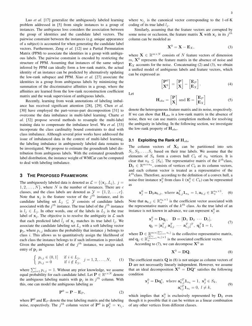
Fig. 2: MCar reassigns the labels for those ambiguously labeledinstances such that instances of the same subjects cohesivelyform potentially-separable convex hulls. The vertices of eachconvex hull are the representatives of each class, forming Dk.The interior and outline of the circles are color-coded to representthree different classes and various ambiguous labels, respectively.

a perfect recovery of ambiguous labeling such that Y∗ = P0.Several factors contribute to our inability to resolve the ambiguity.For instance, if label 1 is consistently present in the candidatelabeling set of each instance, assigning v1 for each column vectorof Y yields a trivial solution. This issue is also addressed in [21],as learning from instances associated with two consistently co-occurring labels is impossible.

Note that Y∗ = P0 is one of the possible optimal solutions to(15). The solution may not be unique if any one of the instancesbelongs to more than one convex hull, i.e. the convex hulls fromdifferent classes overlap with each other. Hence, an instance canbe ideally decomposed from either one of the convex hulls withoutfurther changing the rank of [Y; X0]. This issue is analogous tothe non-separable case of linear support vector machine (SVM).Nevertheless, it is our intention to seek Y = P0 by solving (15)with the understanding that 1) the ambiguous labeling carries ra-tional information, and 2) the feature is sufficiently discriminativesuch that data lies in the feature subspace where convex hulls ofeach class are separable [35].

Figure 2 illustrates the geometric interpretation of MCar us-ing the convex hull representation. When each element in thecandidate labeling set is trivially treated as the true label, theconvex hulls of each class are erroneously expanded and the low-rank assumption of

[Y; X0

]does not hold. MCar exploits the

underlying low-rank structure of[Y; X0

], which is equivalent

to reassigning the labels for those ambiguously labeled instancessuch that instances of the same class cohesively form a convexhull. Hence, each over-expanded convex hull shrinks to its actualcontour, and the convex hulls become potentially separable. This isessentially different from discriminative ambiguous learning meth-ods that construct the hyperplane between ambiguously labeledinstances by minimizing the ambiguous loss.

When data is contaminated by sparse errors, the optimizationproblem in (15) can be reformulated as

minH,EX ,EP

rank(H) + λ‖EX‖0

s.t. H =

[YZ

]=

[PX

]−[EP

EX

],

yj ∈ {v1,v2, . . . ,vc}, j = 1, 2, . . . , N,

yi,j = 0 if i /∈ Lj ∀j,

(16)

where H is the heterogeneous feature matrix in the absenceof noise, and Z is the recovered feature matrix. The parameter

5

= −

𝐏 𝐗

𝐄𝑃

𝐄𝑋 = − 𝐇 =

𝐘𝐙

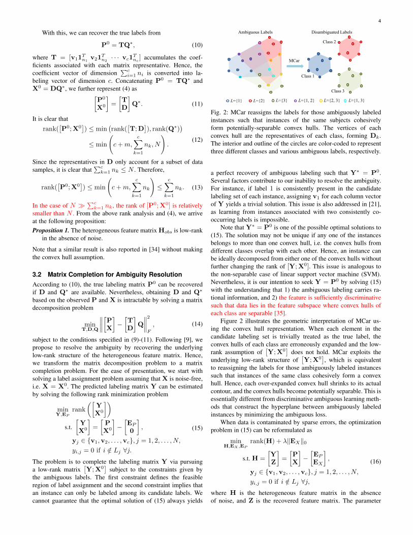
Fig. 3: Ideal decomposition of the heterogeneous feature matrixusing MCar. The underlying low-rank structure and the ambiguouslabeling are recovered simultaneously.

λ ∈ R+ controls the rank of H and the sparsity of noise. Theobjective is to assign the predicted label Y and extract the sparsenoise of X in pursuit of a low-rank H. Figure 3 illustrates theideal decomposition of the heterogeneous feature matrix, wherethe underlying low-rank structure and the ambiguous labels arerecovered simultaneously.

As (16) is a combinatorial optimization problem, we relax eachcolumn vector of Y in probability simplex in Rc. The originalformulation can be rewritten as

minH,EX ,EP

rank(H) + λ‖EX‖0 + γ‖Y‖0

s.t. H =

[YZ

]=

[PX

]−[EP

EX

],

1Tc Y = 1TN , Y ∈ Rc×N+ ,

yi,j = 0 if i /∈ Lj ∀j,

(17)

where γ ∈ R+ encourages the sparsity of Y such that theoriginal discrete feasible region can be well approximated. Fromthe perspective of convex hull representation, such relaxationallows each instance to be represented from more than one setof representative matrix Dk, while it will be penalized by thenon-sparsity of Y. Consequently, the predicted label of instance jcan be obtained as

lj = arg maxi∈Lj

yi,j . (18)

3.3 Ambiguously Labeled Data with Labeling Imbal-anceThe class imbalance may lead to performance degradation in SVMas a majority class with abundant training samples can bias thedecision boundary toward a minority class with scarce trainingsamples. Analogously, MCar may suffer from labeling imbalancewhen a majority label is frequently present among the candidatelabels in the ambiguously labeled data. When we resolve theambiguity using (17), the heterogeneous feature vectors associatedwith a majority label are more likely to dominate the low-rankapproximation of the heterogeneous matrix than those associatedwith a minor label. Hence, the recovered soft labeling matrix willbias toward those soft labeling vectors associated with majoritylabels.

Class-weighted SVM applies unequal weighting to the costfunction of different classes to mitigate the class imbalance [36].Hence, instances from the minority label will be better emphasizedthan those from the dominant label to establish an objectivedecision boundary. However, the concept of class-weighted SVMcannot be directly applied to MCar to deal with label imbalancessince each instance is not labeled as a particular class in the

ambiguously labeled data. Without the knowledge of the truelabels, we formulate the instance-weighted objective function of(14) as

minT,D,Q

N∑j=1

ηj

∥∥∥∥[pjxj

]−[TD

]qj

∥∥∥∥2

F

, (19)

where ηj is the instance weight of the jth instance. In order tobalance the square errors contributed by each class in (19), weaim to set instance weight ηj as 1/Nlj , where Nlj is the numberof the instances from the lj class. Nevertheless, assigning a classweight for each instance is not feasible in the ambiguously labeleddata since the true label lj is not explicitly known. Moreover, Niis intractable since the data is not explicitly labeled. Hence, wepropose to set the instance weight as

ηj =1∑c

i=1 pi,jNi, (20)

where

Ni =N∑j=1

pi,j (21)

is the estimated number of instances of the ith class. The estimatednumber of instances of the ith class accumulates the soft labelingscores corresponding to the ith class across all the instances.With the soft labeling vector pj , we can compute the effectivenumber of instances of the class that the jth instance belongs to by∑ci=1 pi,jNi. Hence, our proposed weighting scheme is eligible

to compute the effective class weight of each ambiguously labeledinstance even though the knowledge of true label is not available.The design of the instance weight is not unique, and readers mayrefer to [11], [37] for modeling the instance weight with respectto various objectives.

For the ease of presentation, we reformulate (19) as

minT,D,Q

∥∥∥∥[PX]

W −[TD

]QW

∥∥∥∥2

F

, (22)

where

W =√

diag(1TNPTP)−1

(23)

is a diagonal weighting matrix with wj,j =√ηj . As post-

multiplying W does not increase the rank of a matrix, we claimthat Proposition 1 also applies to the weighted heterogeneousfeature matrix HobsW = [P; X]W. We propose the weightedMCar (WMCar) by generalizing (17) as

minH,EX ,EP

rank(HW) + λ‖EXW‖0 + γ‖YW‖0

s.t. HW =

[YWZW

]=

[PWXW

]−[EPWEXW

],

1Tc YW = 1TNW, YW ∈ Rc×N+ ,

yi,j = 0 if i /∈ Lj ∀j.

(24)

Let Hobs = HobsW, H = HW, and E = EW, we reformulate(24) as

minH,EP ,EX

rank(H) + λ‖EX‖0 + γ‖Y‖0

s.t. H =

[YZ

]=

[PX

]−[EP

EX

],

1Tc Y = 1TNW, Y ∈ Rc×N+ ,

yi,j = 0 if i /∈ Lj ∀j.

(25)

6

The predicted label can be retrieved from Y = YW−1 using(18). Interestingly, the instance-weighted MCar is equivalent toexecuting MCar with the weighted heterogeneous feature matrix.A larger weight on the heterogeneous feature vectors associatedwith minority labels provides those instances a stronger impact inthe low-rank approximation of the heterogeneous matrix, and thusthe labeling imbalance can be compensated. As (17) is generalizedby (25) in consideration of labeling imbalance, WMCar is identicalto MCar in the special case of W = I.

Algorithm 1 The optimization algorithm for WMCar (29)

Input: P ∈ Rc×N , X ∈ Rm×N , W ∈ RN×N , Lj ∀j, λ, and γ.1: Initialization:2: P = PW, X = XW, Hobs = [P; X];3: Y = 0, Z = 0, µ > 0, µmax > 0, ρ > 1, Λ = [ΛP ; ΛX ] =

Hobs/‖Hobs‖2;4: while not converged do5: EP = P− Sγµ−1 [Y − µ−1ΛP ];6: EX = Sλµ−1 [X− Z + µ−1ΛX ];7: (U,Σ,V) = svd

(Hobs − E + µ−1Λ

);

8: H = USµ−1 [Σ]VT ;9: Λ = Λ + µ

(Hobs − H− E

);

10: µ = min(ρµ, µmax);11: Project Y:12: . Line: 13: Projection for (31)13: yi,j = 0 if i /∈ Lj ∀j;14: . Line: 15-16: Projection for (30)15: Y = max(Y, 0);16: yj = wj,j yj/‖yj‖1, ∀j;17: end while18: H = HW−1, E = EW−1

Output: (H,E)

4 OPTIMIZATION

The augmented Lagrangian method (ALM) has been extensivelyused for solving low-rank problems [14], [38]. In this section, wepropose to incorporate the ALM with the projection step [9], [10]to solve the optimization problem of WMCar.

In order to decouple Y in the first and third terms of theobjective function in (25), we replace ‖Y‖0 with ‖P− EP ‖0 andrewrite (25) as

minH,EX ,EP

rank(H) + λ‖EX‖0 + γ‖P− EP ‖0

s.t. H =

[YZ

]=

[PX

]−[EP

EX

],

1Tc Y = 1TNW, Y ∈ Rc×N+ ,

yi,j = 0 if i /∈ Lj ∀j.

(26)

Following the procedure of ALM, we relax the first constraint in(26) and reformulate it as

minH,E,Λ,µ

`(H, E,Λ, µ)

s.t. 1Tc Y = 1TNW, Y ∈ Rc×N+ ,

yi,j = 0 if i /∈ Lj ∀j,

(27)

where µ ∈ R+ and Λ ∈ R(c+m)×N . The Lagrangian is expressedas`(H, E,Λ,µ) = rank(H) + λ‖EX‖0 + γ‖P− EP ‖0

+⟨Λ, Hobs − H− E

⟩+µ

2

∥∥Hobs − H− E∥∥2

F.

(28)In order to make the optimization problem feasible, we approxi-mate the rank with the nuclear norm and the `0 norm with the `1norm [39]. Thus, we solve the following formulation as the convexsurrogate of (27)

minH,E,Λ,µ

`R(H, E,Λ, µ) (29)

s.t. 1Tc Y = 1TNW, Y ∈ Rc×N+ , (30)

yi,j = 0 if i /∈ Lj ∀j, (31)

where the Lagrangian is represented as

`R(H, E,Λ,µ) =∥∥H∥∥∗ + λ‖EX‖1 + γ‖P− EP ‖1

+⟨Λ, Hobs − H− E

⟩+µ

2

∥∥Hobs − H− E∥∥2

F.

(32)The ALM operates in the sense that H, EP , and EX can be solvedalternately by fixing other variables. In each iteration, we employa similar projection technique used in [9], [10] to enforce Y tobe feasible. The entire procedure for solving (29) is summarizedin Algorithm 1, and the details of the optimization algorithm arepresented in the following paragraphs.

4.1 Solving for EP

To update EP , we fix H, EX , Λ and µ obtained in the previousiteration. Hence, the problem for updating EP can be solved byfirst computing

E∗P = argminEP

γ‖P− EP ‖1 +⟨ΛP , P− Y − EP

⟩+µ

2

∥∥P− Y − EP

∥∥2

F.

(33)

For the ease of derivation, we let B = P− EP and update B assurrogate. We can reformulate (33) as

B∗ = argminB

γ‖B‖1 +⟨ΛP , B− Y

⟩+µ

2

∥∥B− Y∥∥2

F,

= argminB

γ‖B‖1 +µ

2‖B− Y + µ−1ΛP ‖2F ,

= argminB

γ‖B‖1 +µ

2‖Y − µ−1ΛP − B‖2F .

(34)Using the subgradient of (34), we can obtain the closed-form

solution for updating B

B∗ = Sγµ−1 [Y − µ−1ΛP ]. (35)

Consequently, we can update EP as

E∗P = P− B∗ = P− Sγµ−1 [Y − µ−1ΛP ]. (36)

4.2 Solve EX

To update EX , we fix H, EP , Λ and µ obtained in the previousiteration. Thus, the problem for updating EX can be solved by

E∗X = argminEX

λ‖EX‖1 +⟨ΛX , X− Z− EX

⟩+µ

2

∥∥X− Z− EX

∥∥2

F,

= argminEX

λ‖EX‖1 +µ

2‖X− Z + µ−1ΛX − EX‖2F .

(37)

7

Using the subgradient of (37), we can obtain the closed-formsolution for updating EX

E∗X = Sλµ−1 [X− Z + µ−1ΛX ]. (38)

4.3 Solve H

To update H, we fix EP , EX , Λ and µ obtained in the previousiteration. The feasible region of Y in H is currently not consideredbut will be handled in the projection step of Y (Section 4.4).Therefore, the problem for updating H can be solved by

H∗ = argminH‖H‖∗ +

⟨Λ, Hobs − H− E

⟩(39)

+µ

2

∥∥Hobs − H− E∥∥2

F, (40)

= argminH‖H‖∗ +

µ

2‖AH − H‖2F , (41)

where AH = Hobs − E + µ−1Λ. According to [40], the aboveproblem can be solved by

H∗ = USµ−1 [Σ]VT , (42)

where Σ can be obtained from the singular value decomposition(SVD) of AH denoted as (U,Σ,V) = svd (AH) . Followingthe procedure in the augmented Lagrangian method (ALM), wecan update Λ and µ as

Λ = Λ + µ(Hobs − H− E

), (43)

where µ = min(ρµ, µmax), in each iteration based on the updatedEP , EX , and H.

4.4 Project Y

Since the SVD operation for solving H does not always return afeasible Y, we use a projection technique similar to the one in [9],[10] to enforce Y to be feasible in each iteration. The projectioninvolves two steps. First, we enforce those entries of Y that donot correspond to the candidate labels to be zeros since the actuallabel only comes from the candidate labeling set provided by theambiguous labels. Second, each column vector of Y = YW−1

is constrained to be in the probability simplex. As a result, wereplace those negative entries in Y with zeros and then normalizeeach column yj so that the summation of the entries in yj is equalto wj,j .

Algorithm 2 The algorithm for WMCar-ICE

Input: P ∈ Rc×N , X ∈ Rm×N , Lj ∀j.1: while A 6= ∅ and within the maximum number of iterations

do2: W =

√diag(1TNPTP)

−1

;3: Obtain Y using WMCar (Algorithm 1);4: Eliminate the least likely candidate in Lj , j ∈ E using

(44)-(47);5: . Line: 6-7: Project Y to comply with Lj ,∀j6: yi,j = 0, if i /∈ Lj ∀j;7: yj = yj/‖yj‖1 ∀j;8: P← Y;9: end while

Output: (H,E)

5 ITERATIVE CANDIDATE ELIMINATION FOR AMBI-GUITY RESOLUTION

According to (23), the weighting matrix W of WMCar is afunction of P. As WMCar resolves the label ambiguity in P, therecovered soft labeling matrix Y can provide a better estimate ofW than the original P. This motivates us to iteratively resolve theambiguity by alternating between recovering Y and updating W.Nevertheless, the performance of iterative WMCar is not steady asshown in Figure 11. We propose WMCar with ICE (WMCar-ICE)to resolve the ambiguity by WMCar and then remove the leastlikely candidate labels in each iteration. The least likely candidatelabel of the jth instance is denoted as

m(j) = argmini∈Lj

yi,j , (44)

and its corresponding soft labeling score is denoted as ym(j),j .As removing a candidate label, which is actually a true label, inthe candidate set generates an irreversible error, we propose toiteratively remove a portion of the least likely candidate labelsthat have relatively low soft labeling scores than others.

Let A denote the set consisting of the indices of thoseinstances that have more than one candidate label, which isrepresented as

A = {j | |Lj | > 1,∀j}. (45)

We define the elimination factor as fe (0 ≤ fe ≤ 1), whichaccounts for the proportion of instances in A participating inthe candidate elimination. We construct a subset E of A, whichconsists of the entries that correspond to the smallest fe portionof {ym(j),j |j ∈ A}. We represent it as

E = {j | ym(j),j ≤ t, j ∈ A}. (46)

Note that t is automatically determined such that |E| = dfe |A|e.Hence, we can update the candidate labeling sets by

Lj ← Lj − {m(j)}, j ∈ E . (47)

We enforce the soft labeling matrix Y to comply with theupdated candidate labeling sets. We set yi,j = 0, if i /∈ Lj ∀j andproject each column vector of Y in the probability simplex. Theoriginal P will be replaced by Y, which will serve as the inputof WMCar in the next iteration. The procedure of WMCar-ICEis summarized in Algorithm 2. Note that updating the weightingmatrix W is an important step in WMCar-ICE since it adaptivelyadjusts the importance among instances based on the updated Yin the previous iteration. This ICE procedure can be utilized byother ambiguous learning techniques that adopt the soft labelinginput/output similar to that of WMCar.

6 LABELING CONSTRAINTS BETWEEN INSTANCES

In practical applications, several ambiguously labeled instancescan appear in the same venue. As a result, pairwise relationsbetween instances can be utilized to assist ambiguity resolution.For example, two persons in a news photo should not be identifiedas the same subject even though both of them are ambiguouslylabeled in the caption. Such prior knowledge can be easily incor-porated by restricting the feasible region of the labeling matrix.Moreover, it is essential to handle the open set problem, wherethere are some instances whose identities never appear in thelabels. These unrecognized instances can be treated as the nullclass.

8

In this section, we show how MCar’s formulation can beextended to associate the identities in news photos when thenames are provided in captions. We assume all the instances (faceimages) are collected from the K groups (photos), and Gk isthe set of indices of the instances (face images) appearing in thekth group (photo). Note that instances (face images) from thesame group (photo) share the same ambiguous labels provided bytheir associated caption. Without loss of generality, we assumethat the cth class corresponds to the null class. Considering theprior knowledge, the original formulation given in (17) can bereformulated as

minH,EX ,EP

rank(H) + λ‖EX‖0 + γ‖Y‖0 (48)

s.t. H =

[YZ

]=

[PX

]−[EP

EX

],

1Tc Y = 1TN , Y ∈ Rc×N+ , (49)

yi,j = 0 if i /∈ Lj , i = 1, 2, . . . , c− 1, ∀j, (50)∑j∈Gk

c−1∑i=1

yi,j ≥ 1 if ∪j∈Gk

Lj 6= {c},∀k, (51)∑j∈Gk

yi,j ≤ 1, i = 1, 2, . . . , c− 1, ∀k. (52)

Constraints (49) and (50) are inherited from the original formu-lation. The constraint in (51), assumes that there is at least onenon-null identity in a photo unless all the instances in a photo areexplicitly labeled as null. This constraint is enforced to avoid thetrivial solution that all the instances are treated as belonging tothe null class. A similar constraint has been considered by [17]and [12] via restricting the candidate labeling set and confiningthe feasible space of PPM, respectively. The constraint in (52)enforces the uniqueness of non-null identities. Note that thisframework can be easily tailored to handle other prior knowledge(e.g. must/cannot-link constraints, prior statistics) by regularizingthe labeling matrix. This problem can be solved by following thesimilar relaxation procedures for solving (17). The optimizationprocedure is summarized in Algorithm 3.

Following the relaxation procedure in Section 4, we canreformulate (48) as

minH,E,Λ,µ

‖H‖∗ + λ‖EX‖1 + γ‖P−EP ‖1

+ 〈Λ,Hobs −H−E〉+µ

2‖Hobs −H−E‖2F ,

(53)

s.t. 1Tc Y = 1TN , Y ∈ Rc×N+ , (54)

yi,j = 0 if i /∈ Lj , i = 1, 2, . . . , c− 1, ∀j, (55)∑j∈Gk

c−1∑i=1

yi,j ≥ 1 if ∪j∈Gk

Lj 6= {c},∀k, (56)∑j∈Gk

yi,j ≤ 1, i = 1, 2, . . . , c− 1, ∀k. (57)

We use a similar procedure of Algorithm 1 presented in Section4 to solve (53). We again use the projection method to guide theprocess of the matrix completion such that the constraints on Yare satisfied. Additionally, the projection of Y handles the groupconstraints such that the labeling constraints between instances aresatisfied. Hence, we project Y to the feasible regions indicated by(55), (56), and (57) one at a time, and each one is followed by theprojection onto the feasible region indicated by (54) to ensure that

each column of Y lies in the probability simplex. The detailedprocedure is summarized in Algorithm 3. This algorithm can beeasily extended to handle ambiguously labeled data with labelingimbalance by taking H as input with proper manipulation on theprojection steps of Y.

Algorithm 3 The optimization algorithm for (53)

Input: P ∈ Rc×N , X ∈ Rm×N , Lj ∀j, Gk ∀k, λ, and γ.1: Initialization: Y = 0, Z = 0, µ > 0, µmax > 0, ρ > 1,

Λ = [ΛP ; ΛX ] = Hobs/‖Hobs‖2;2: while not converged do3: EP = P− Sγµ−1 [Y − µ−1ΛP ];4: EX = Sλµ−1 [X− Z + µ−1ΛX ];5: (U,Σ,V) = svd

(Hobs −E + µ−1Λ

);

6: H = USµ−1 [Σ]VT ;7: Λ = Λ + µ (Hobs −H−E);8: µ = min(ρµ, µmax);9: Project Y:

10: . Line: 11-13: Projection for (55) and (54)11: Y = max(Y, 0);12: yi,j = 0 if i /∈ Lj , i = 1, 2, . . . , c− 1,∀j ;13: yj = yj/‖yj‖1, ∀j;14: . Line: 15-22: Projection for (56) and (54)15: for k = 1 : K do16: if ∪j∈Gk

Lj 6= {c} then17: for i = 1 : c− 1, j ∈ Gk do18: yi,j = yi,j/min(

∑g∈Gk

∑c−1i=1 yi,g, 1);

19: end for20: end if21: end for22: yj = yj/‖yj‖1, ∀j;23: . Line: 24-29: Projection for (57) and (54)24: for k = 1 : K do25: for i = 1 : c− 1, j ∈ Gk do26: yi,j = yi,j/max(

∑g∈Gk

yi,g, 1);27: end for28: end for29: yj = yj/‖yj‖1, ∀j;30: end whileOutput: (H,E)

7 EXPERIMENTAL RESULTS

We use the Labeled Faces in the Wild (LFW) dataset [41] and theCMU PIE dataset with synthesized ambiguous labels to evaluatethe performance of our method under various controlled parametersettings. Furthermore, we use the Lost dataset [5] and the LabeledYahoo! News dataset [1], [42] to demonstrate the effectivenessof our method in real-world applications. For the LFW, CMUPIE, and Lost datasets, we use face images in gray scale of range[0, 1.0]. Each instance is preprocessed with histogram equalizationand converted into a column feature vector.

7.1 ParametersIt is interesting to observe that (16) becomes asymptotically sim-ilar to the formulation of Robust Principle Component Analysis(RPCA) [14] as the dimension of the data feature is far greaterthan the number of classes. Motivated by this fact, we fix λ as

λo =1√

max(c+m,N), (58)

9

which is the tradeoff parameter suggested in RPCA. γ is a tuningparameter that controls the sparsity of the soft labeling vectors.For MCar-based methods, we use γ = 2λ0 to encourage strongersparsity of the labeling vector than that of feature noise. For ICE,we set the elimination factor fe as 0.5, and set the maximumnumber of iterations as 5. These parameters yield good results ingeneral, and we will investigate the sensitivity of parameters inSection 7.4.

7.2 Experiments with the Synthesized Dataset

We conduct two types of controlled experiments suggested in[21]. For the inductive experiment, the dataset is evenly split intoambiguously labeled training set and unlabeled testing set. Theproposed methods, MCar/WMCar-SVM and WMCar-ICE-SVM,learn a multi-class linear SVM [43] with the disambiguated labelsprovided by MCar/WMCar and WMCar-ICE, respectively. Thetesting data is then classified using the learned classifier. For thetransductive experiment, all the data is used as the ambiguouslylabeled training set.

We follow the ambiguity model defined in [21] to generate am-biguous labels in the controlled experiment. Note that α denotesthe number of extra labels for each instance, and β represents theportion of the ambiguously labeled data among all the instances.The degree of ambiguity ε indicates the maximum probabilitythat an extra label co-occurs with a true label, over all labelsand instances. Each controlled experiment is repeated 20 times.We report the average testing (labeling) error rate for inductive(transductive) experiment, where the testing (labeling) error rateis the ratio of the number of erroneously labeled instances to thetotal number of instances in the testing (training) set. The standarddeviations are plotted as error bars in the figures.

We compare the proposed MCar-based methods with sev-eral state-of-the-art ambiguous learning approaches for singleinstances with ambiguous labeling: CLPL [21], DLHD/DLSD[7], KDLSD [13], and IPAL [25]. We report the performance ofthese methods when the experimental results are available in theirpapers. Otherwise, we use the configuration suggested in theirpapers to conduct the experiments. We use ‘naive’ [21] as thebaseline method, which learns a classifier from minimizing thetrivial 0/1 loss.

7.2.1 The LFW DatasetThe FIW(10b) dataset [21] consists of the top 10 most frequentsubjects selected from the LFW dataset [41], and the first 50 faceimages of each subject are used for evaluation. We use the croppedand resized face images readily provided by the authors of [21],where the face images are of 45× 55 pixels.

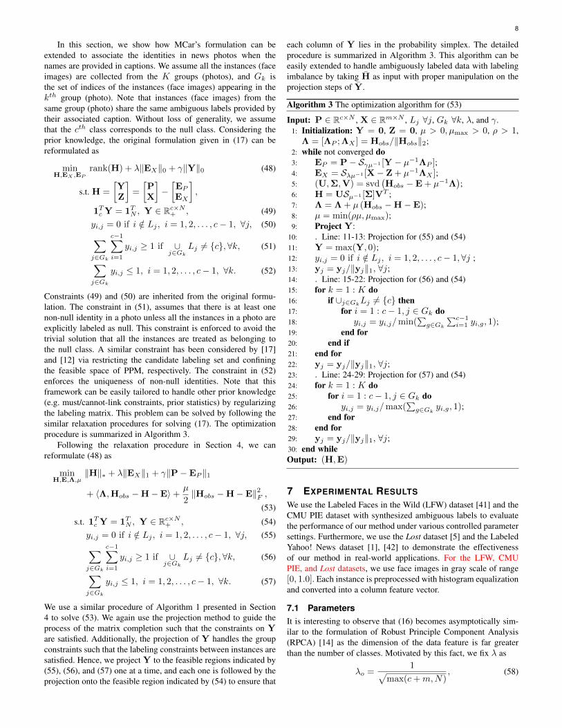
Figures 4a and 4b show the results of the inductive experi-ments. Figure 4a shows that the MCar-based methods significantlyoutperform all the other methods when the portion of ambiguouslylabeled data is larger than 0.2. The performance of WMCaris comparable to that of MCar since the ambiguously labeleddata generated by this ambiguity model does not substantiallyresult in labeling imbalance. WMCar-ICE demonstrates betterperformance than MCar and WMCar when more than 0.7 portionsof the instances are ambiguously labeled. An explanation is thatICE eliminates the candidates based on the ordering of the leastsoft labeling score of each instance. This prioritization step caneffectively benefit from a large portion of ambiguously labeledsamples (i.e., large α) that usually carries a diverse aspect of soft

labeling scores. When the portion of ambiguously labeled samplesis small, the improvement due to ICE becomes insignificant.

Figure 4b shows that MCar outperforms prior methods overvarious degrees of ambiguity except when ε > 0.7. Thus, MCaryields improved performance at low and intermediate levels ofambiguity, but it becomes susceptible at high levels of ambiguity.One explanation is that both the true label and the extra labels ofa subject will result in low-rank component of the labeling matrixwhen they are likely to co-occur in high degree of ambiguity.Consequently, separating the true label from the extra labels inMCar becomes challenging. Another explanation is that a highdegree of ambiguity results in labeling imbalance, which causesthe performance degradation of MCar. To verify this, we obtain thelabel distribution by counting the number of label occurrences inthe candidate labeling sets for each class. We define the imbalancefactor as the ratio of the maximum to the minimum value inthe label distribution. The average imbalance factor varies from1.33 to 3.58 as the degree of ambiguity increases. This confirmsthat WMCar outperforms MCar in high degree of ambiguity sinceWMCar is effective in mitigating the impact of labeling imbalance.Furthermore, WMCar-ICE outperforms WMCar by iterativelyremoving the least likely candidate labels from the candidatelabeling sets. This experiment demonstrates that the labelingimbalance can cause performance degradation even though thereis no class imbalance among the number of groundtruth faces perclass.

In Figure 4c, MCar-based methods outperform the otherapproaches only when the number of extra labels is less than5 in the transductive experiment. This shows that MCar-basedmethods cannot be effective when the labeling is severely clutteredsuch that the low-rank approximation of heterogeneous featurefails. Similar to the controlled parameter setting in Figure 4a,the ambiguously labeled data generated by this ambiguity modeldoes not substantially result in labeling imbalance. Hence, theperformance of WMCar is comparable to that of MCar, andWMCar-ICE slightly outperforms WMCar.

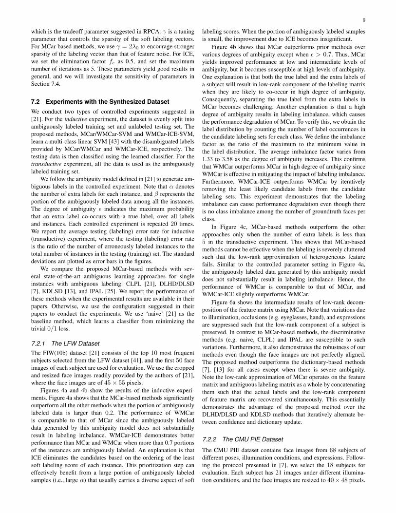
Figure 6a shows the intermediate results of low-rank decom-position of the feature matrix using MCar. Note that variations dueto illumination, occlusions (e.g. eyeglasses, hand), and expressionsare suppressed such that the low-rank component of a subject ispreserved. In contrast to MCar-based methods, the discriminativemethods (e.g. naive, CLPL) and IPAL are susceptible to suchvariations. Furthermore, it also demonstrates the robustness of ourmethods even though the face images are not perfectly aligned.The proposed method outperforms the dictionary-based methods[7], [13] for all cases except when there is severe ambiguity.Note the low-rank approximation of MCar operates on the featurematrix and ambiguous labeling matrix as a whole by concatenatingthem such that the actual labels and the low-rank componentof feature matrix are recovered simultaneously. This essentiallydemonstrates the advantage of the proposed method over theDLHD/DLSD and KDLSD methods that iteratively alternate be-tween confidence and dictionary update.

7.2.2 The CMU PIE Dataset

The CMU PIE dataset contains face images from 68 subjects ofdifferent poses, illumination conditions, and expressions. Follow-ing the protocol presented in [7], we select the 18 subjects forevaluation. Each subject has 21 images under different illumina-tion conditions, and the face images are resized to 40× 48 pixels.

10

0 0.2 0.4 0.6 0.8 120

30

40

50

60

70

80

90

100

Portion of ambiguously labeled samples (α)

Avera

ge test err

or

rate

(%

)

naive

CLPL

DLHD

DLSD

KDLSD

IPAL

MCar−SVM

WMCar−SVM

WMCar−ICE−SVM

(a)

0 0.2 0.4 0.6 0.8 120

30

40

50

60

70

80

90

100

Degree of ambiguity (ε)

Avera

ge test err

or

rate

(%

)

naive

CLPL

DLHD

DLSD

KDLSD

IPAL

MCar−SVM

WMCar−SVM

WMCar−ICE−SVM

(b)

0 2 4 6 8 100

20

40

60

80

100

Number of extra labels for each ambiguously labeled sample (β)

Avera

ge labelin

g e

rror

rate

(%

)

naive

CLPL

DLHD

DLSD

KDLSD

IPAL

MCar

WMCar

WMCar−ICE

(c)

Fig. 4: Performance comparisons on the FIW(10b) dataset. (a) α ∈ [0, 0.95], β = 2, inductive experiment. (b) α = 1.0, β = 1,ε ∈ [1/(c− 1), 1], inductive experiment. (c) α = 1.0, β ∈ [0, 1, . . . , 9], transductive experiment.

We synthesize the ambiguous labels based on the controlledparameters. The results of two transductive experiments for CMUPIE dataset are shown in Figures 5a and 5b. In Figure 5a, MCar-based methods and IPAL recover all the label ambiguity forvarious portions of ambiguously labeled samples. In Figure 5b,our proposed methods consistently outperform most of the state-of-the-art methods except IPAL as we increase the number of extralabels for each ambiguously labeled sample. Since the CMU PIEdataset is collected in a constrained environment, the collectiveface images of a subject are well-modeled by low-rank approxi-mation. Hence, MCar demonstrates marginally improvements overmost of the methods in this dataset. This can be seen by visualizingthe intermediate results of low-rank decomposition of the featurematrix using MCar as shown in Figure 6b. Besides, the IPALmethod outperforms our methods when β > 6. Since the IPALmethod utilizes the locally linear embedding for label propagation,which is effective in learning the underlying structure of data thathas plenty of samples collected in the constrained environment.Hence, IPAL is able to recover the severely cluttered labels thatMCar-based methods fail to approximate it as a low-rank matrix.

7.3 Experiments with Real-world DatasetWe conduct experiments on the Lost dataset and Labeled Yahoo!News dataset where the ambiguous labeling are collected in thereal world. In the Labeled Yahoo! News dataset, we consider thelabeling constraints between instances.

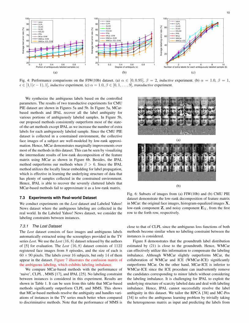
7.3.1 The Lost DatasetThe Lost dataset consists of face images and ambiguous labelsautomatically extracted using the screenplays provided in the TVseries Lost. We use the Lost (16, 8) dataset released by the authorsof [5] for evaluation. The Lost (16, 8) dataset consists of 1122registered face images from 8 episodes, and the size of each is60× 90 pixels. The labels cover 16 subjects, but only 14 of themappear in the dataset. Figure 7 illustrates the confusion matrix ofthe ambiguous labeling, which exhibits labeling imbalance.

We compare MCar-based methods with the performance of‘naive’, CLPL , MMS [17], and IPAL [25]. No labeling constraintbetween instances is considered in this experiment. Results areshown in Table 1. It can be seen from this table that MCar-basedmethods significantly outperform CLPL and MMS. This showsthat MCar-based methods resolve the ambiguity and handles vari-ations of instances in the TV series much better when comparedto discriminative methods. Note that the performance of MMS is

(a)

(b)

Fig. 6: Subsets of images from (a) FIW(10b) and (b) CMU PIEdataset demonstrate the low-rank decomposition of feature matrixin MCar: the original face images, histogram-equalized images X,low-rank component Z, and noisy component EX , from the firstrow to the forth row, respectively.

close to that of CLPL since the ambiguous loss functions of bothmethods become similar when no labeling constraint between theinstances is considered.

Figure 8 demonstrates that the groundtruth label distributionestimated by (21) is close to the groundtruth. Hence, WMCarcan effectively utilize this information to compensate the labelingimbalance. Although WMCar slightly outperforms MCar, thecollaboration of WMCar and ICE (WMCar-ICE) significantlyoutperforms MCar. On the other hand, MCar-ICE is inferior toWMCar-ICE since the ICE procedure can inadvertently removethe candidates corresponding to minor labels without consideringthe labeling imbalance. It is challenging for IPAL to exploit theunderlying structure of scarcity labeled data and deal with labelingimbalance. Hence, IPAL cannot successfully resolve the labelambiguity in this dataset. We tailor the RPCA [38] and MC-Pos[34] to solve the ambiguous learning problem by trivially takingthe heterogeneous matrix as input and predicting the labels from

11

0 0.2 0.4 0.6 0.8 10

1

2

3

4

5

6

7

Portion of ambiguously labeled samples (α)

Avera

ge labelin

g e

rror

rate

(%

)

naive

CLPL

DLHD

DLSD

KDLSD

IPAL

MCar

WMCar

WMCar−ICE

(a)

0 2 4 6 8 100

20

40

60

80

100

Number of extra labels for each ambiguously labeled sample (β)

Avera

ge labelin

g e

rror

rate

(%

)

naive

CLPL

DLHD

DLSD

KDLSD

IPAL

MCar

WMCar

WMCar−ICE

(b)

Fig. 5: Performance comparisons on the CMU PIE dataset. (a) α ∈ [0, 0.95], β = 2, transductive experiment. (b) α = 1.0,β ∈ [0, 1, . . . , 9], transductive experiment.

1 2 3 4 5 6 7 8 9 10 11 12 13 14 15 16

1

2

3

4

5

6

7

8

9

10

11

12

13

14

15

16

99.17

35.50

11.33

11.83

15.67

13.33

2.33

2.33

1.17

4.00

2.50

0.67

0.00

0.00

0.00

0.00

30.83

94.33

2.00

31.50

2.00

13.00

5.17

0.50

0.00

0.00

1.33

0.00

0.33

0.00

0.00

0.00

7.00

7.00

67.17

0.67

19.00

0.50

28.33

0.33

0.00

5.33

0.00

0.00

0.33

0.00

0.00

0.00

11.17

39.67

0.00

48.33

0.00

6.33

0.33

0.00

0.00

0.00

0.00

0.00

1.67

2.33

0.00

0.00

33.00

4.00

25.67

0.00

43.50

3.67

0.00

0.00

0.00

1.83

7.00

0.00

0.00

0.33

0.00

0.00

9.50

11.50

0.33

5.50

1.33

47.67

0.67

2.00

0.00

0.00

1.50

0.67

5.67

0.67

0.00

0.00

3.00

2.33

19.50

0.67

0.33

0.67

39.17

0.00

0.00

0.00

0.00

0.00

0.00

0.00

0.00

0.00

0.67

1.00

0.83

0.00

0.00

2.33

0.00

14.83

13.83

1.83

0.00

4.50

0.33

5.00

0.00

0.00

0.33

1.00

0.00

0.00

0.00

0.00

0.00

7.00

35.50

0.00

0.00

3.33

0.00

0.00

0.00

0.00

5.17

0.00

9.33

0.50

0.00

2.00

0.00

2.50

0.00

10.00

0.00

0.67

1.00

1.67

0.00

0.00

2.17

1.67

0.00

1.67

5.50

1.67

0.00

0.67

0.00

0.00

12.33

0.00

4.50

0.33

0.00

0.00

1.33

0.00

0.00

0.00

0.00

1.33

0.00

0.33

10.50

0.67

0.00

8.17

0.00

1.00

0.00

0.00

0.33

0.00

0.00

0.50

0.00

8.83

0.00

0.00

0.00

0.00

1.33

0.00

11.17

0.00

0.00

0.00

0.00

0.00

0.00

1.50

0.67

1.67

0.00

2.50

0.00

1.00

0.00

0.00

0.00

8.67

0.00

0.00

0.00

0.00

5.50

0.00

0.00

0.00

0.00

0.00

0.00

0.00

0.00

0.00

0.00

0.00

0.00

0.00

0.33

0.00

0.33

0.33

0.00

0.00

0.00

0.00

0.00

0.33

0.00

0.00

0.00

0.00

0.00

0.00

204

83

32

28

34

34

5

7

3

12

5

2

0

0

0

0

75

198

5

72

6

35

11

1

0

0

4

0

1

0

0

0

20

19

142

2

39

1

58

1

0

14

0

0

1

0

0

0

29

89

0

103

0

19

1

0

0

0

0

0

4

5

0

0

71

12

54

0

88

9

0

0

0

4

14

0

0

1

0

0

24

31

1

16

4

103

2

6

0

0

4

2

12

2

0

0

7

6

40

2

1

2

76

0

0

0

0

0

0

0

0

0

2

2

2

0

0

7

0

33

29

5

0

10

1

12

0

0

1

3

0

0

0

0

0

14

61

0

0

7

0

0

0

0

15

0

26

1

0

6

0

7

0

25

0

2

3

4

0

0

5

5

0

4

11

5

0

2

0

0

26

0

11

1

0

0

4

0

0

0

0

4

0

1

23

2

0

18

0

3

0

0

1

0

0

1

0

19

0

0

0

0

3

0

25

0

0

0

0

0

0

3

2

5

0

6

0

2

0

0

0

20

0

0

0

0

12

0

0

0

0

0

0

0

0

0

0

0

0

0

1

0

1

1

0

0

0

0

0

1

0

0

0

0

0

0

Ambiguously labeled as

Gro

un

dtr

uth

Fig. 7: The confusion matrix of the ambiguous labeling in Lost(16, 8) dataset. The upper number of each square accounts for thenumber of occurrences of a candidate label, whereas the lowernumber of each square is computed by accumulating the softlabeling score of each occurrence of a candidate label.

the soft labeling matrix of output with (18). The experimentalresult shows that existing low-rank approximation methods cannotsubstantially resolve the label ambiguity.

7.3.2 The Labeled Yahoo! News Dataset

The Labeled Yahoo! News dataset contains fully annotated facesin the images with names in the captions. It consists of 31147detected faces from 20071 images. We use the precomputed SIFTfeature of dimension 4992 extracted from that face images pro-vided by Guillaumin et al. [42]. Following the protocol suggestedin [17], we retain the 214 subjects with at least 20 occurrencesin the captions. The remaining face images and names are treatedas belonging to the additional null class. The ambiguous labelingis imbalanced in this dataset, where the number of labels present

1 2 3 4 5 6 7 8 9 10 11 12 13 14 15 160

100

200

300

400

Num

ber

of in

stan

ces

Class

GroundtruthEstimated

Fig. 8: The groundtruth label distribution of the Lost (16, 8)dataset. ‘Groundtruth’ denotes the number of instances per classcounted from the groundtruth labels, and ‘Estimated’ denotes theestimate of the groundtruth label distribution from the ambiguouslabels.

Method Error Rate

naive 18.6 %CLPL [21] 12.6 %MMS [17] 11.4 %IPAL [25] 22.9 %

RPCA [38] 29.9 %MC-Pos [34] 23.6 %

MCar 8.5 %WMCar 8.2 %MCar-ICE 8.0 %WMCar-ICE 5.2 %

TABLE 1: Labeling error rates for the Lost (16, 8) dataset (avail-able at http://www.timotheecour.com/tv data/tv data.html).

in the captions ranges from 20 to 1917 with mean and standarddeviations equal to 64.6 and 147.3, respectively. The top twosubjects that are present most frequently in the captions are‘george w bush’ and ‘saddam hussein’. We conduct experimentson five training/testing splits by randomly selecting 80% of imagesand their associated captions as training set, and the rest are usedas testing set. In each split, we also maintain the ratio between thenumber of training and testing instances from each subject.

The baseline approaches are CL-SVM, MIMLSVM [44],and MM-SVM [1]. The implementation details of CL-SVM andMIMLSVM are provided in [17]. We implemented the maximal

12

Method Error Rate

CL-SVM 23.1 % ± 0.6 %MIMLSVM [44] 25.3 % ± 0.3 %MM-SVM [1] 21.9 % ± 1.0 %MMS [17] 14.3 % ± 0.5 %LR-SVM [12] 19.2 % ± 0.4 %

MCar-SVM 14.5 % ± 0.4 %WMCar-SVM 13.6 % ± 0.8 %MCar-ICE-SVM 15.0 % ± 1.0 %WMCar-ICE-SVM 12.9 % ± 0.8 %

TABLE 2: Average testing error rates for the Labeled Yahoo!News dataset (available at http://lear.inrialpes.fr/data).

λ/λ0

0 0.5 1 1.5 2 2.5 3 3.5 4

Labelin

g e

rror

rate

(%

)

5

10

15

20

25

30

35

40

45

γ/λ0 = 0.5

γ/λ0 = 1

γ/λ0 = 2

γ/λ0 = 3

γ/λ0 = 4

Fig. 9: Labeling error rates of WMCar evaluated with a set ofparameters (λ, γ) in the Lost (16, 8) dataset.

likelihood assignment (MM) [1] to resolve the label ambiguity inthe training data and train a multi-class linear SVM [43] to classifythe testing data. For fair comparison, the language modeling ofnews captions in [1] is not included in the implementation. Wecompare with two state-of-the-art ambiguous labeling methodsthat consider labeling constraints between instances: MMS [17]and LR-SVM [12], which are based on discriminative model andlow-rank framework, respectively. We resolve the ambiguity forthe labels in the training set using (48) and train a multi-classlinear SVM [43] to classify the testing data. Our MCar-SVMalgorithm exhibits a slightly 0.2% higher error rate as comparedto MMS. An explanation is that MCar relying on the low-rankapproximation for ambiguity resolution is particularly sensitive tolabeling imbalance. This results in performance degradation in thelearned classifier since the output labels of MCar are potentiallybiased toward the majority labels.

Compared to the LR-SVM method, the MCar-SVM algorithmdemonstrates 4.7% improvement on the testing accuracy. SinceMCar assigns the labels across all instances via low-rank approx-imation of heterogeneous feature matrix, it is more effective thanthe LR-SVM method, which updates the PPM and the low-ranksubspace of each class alternately. When we consider the labelingimbalance and utilize the ICE procedure, our proposed WMCar-ICE-SVM outperforms MCar-SVM by 1.6%

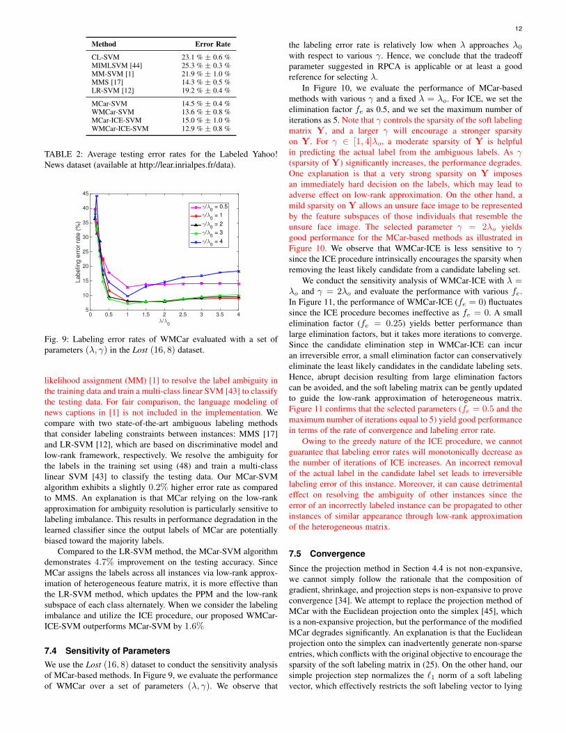
7.4 Sensitivity of ParametersWe use the Lost (16, 8) dataset to conduct the sensitivity analysisof MCar-based methods. In Figure 9, we evaluate the performanceof WMCar over a set of parameters (λ, γ). We observe that

the labeling error rate is relatively low when λ approaches λ0

with respect to various γ. Hence, we conclude that the tradeoffparameter suggested in RPCA is applicable or at least a goodreference for selecting λ.

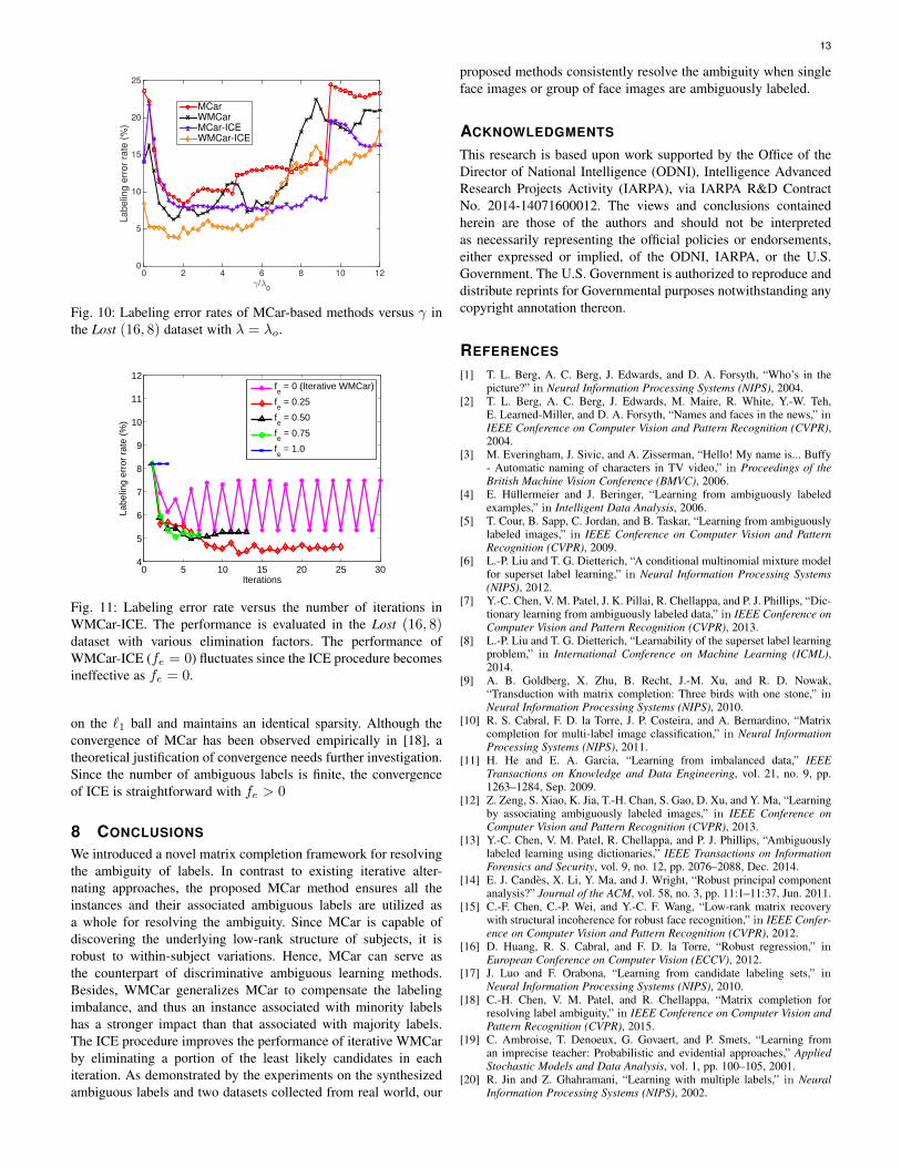
In Figure 10, we evaluate the performance of MCar-basedmethods with various γ and a fixed λ = λo. For ICE, we set theelimination factor fe as 0.5, and we set the maximum number ofiterations as 5. Note that γ controls the sparsity of the soft labelingmatrix Y, and a larger γ will encourage a stronger sparsityon Y. For γ ∈ [1, 4]λo, a moderate sparsity of Y is helpfulin predicting the actual label from the ambiguous labels. As γ(sparsity of Y) significantly increases, the performance degrades.One explanation is that a very strong sparsity on Y imposesan immediately hard decision on the labels, which may lead toadverse effect on low-rank approximation. On the other hand, amild sparsity on Y allows an unsure face image to be representedby the feature subspaces of those individuals that resemble theunsure face image. The selected parameter γ = 2λo yieldsgood performance for the MCar-based methods as illustrated inFigure 10. We observe that WMCar-ICE is less sensitive to γsince the ICE procedure intrinsically encourages the sparsity whenremoving the least likely candidate from a candidate labeling set.

We conduct the sensitivity analysis of WMCar-ICE with λ =λo and γ = 2λo and evaluate the performance with various fe.In Figure 11, the performance of WMCar-ICE (fe = 0) fluctuatessince the ICE procedure becomes ineffective as fe = 0. A smallelimination factor (fe = 0.25) yields better performance thanlarge elimination factors, but it takes more iterations to converge.Since the candidate elimination step in WMCar-ICE can incuran irreversible error, a small elimination factor can conservativelyeliminate the least likely candidates in the candidate labeling sets.Hence, abrupt decision resulting from large elimination factorscan be avoided, and the soft labeling matrix can be gently updatedto guide the low-rank approximation of heterogeneous matrix.Figure 11 confirms that the selected parameters (fe = 0.5 and themaximum number of iterations equal to 5) yield good performancein terms of the rate of convergence and labeling error rate.

Owing to the greedy nature of the ICE procedure, we cannotguarantee that labeling error rates will monotonically decrease asthe number of iterations of ICE increases. An incorrect removalof the actual label in the candidate label set leads to irreversiblelabeling error of this instance. Moreover, it can cause detrimentaleffect on resolving the ambiguity of other instances since theerror of an incorrectly labeled instance can be propagated to otherinstances of similar appearance through low-rank approximationof the heterogeneous matrix.

7.5 Convergence

Since the projection method in Section 4.4 is not non-expansive,we cannot simply follow the rationale that the composition ofgradient, shrinkage, and projection steps is non-expansive to proveconvergence [34]. We attempt to replace the projection method ofMCar with the Euclidean projection onto the simplex [45], whichis a non-expansive projection, but the performance of the modifiedMCar degrades significantly. An explanation is that the Euclideanprojection onto the simplex can inadvertently generate non-sparseentries, which conflicts with the original objective to encourage thesparsity of the soft labeling matrix in (25). On the other hand, oursimple projection step normalizes the `1 norm of a soft labelingvector, which effectively restricts the soft labeling vector to lying

13

γ/λ0

0 2 4 6 8 10 12

Labelin

g e

rror

rate

(%

)

0

5

10

15

20

25

MCarWMCarMCar-ICEWMCar-ICE

Fig. 10: Labeling error rates of MCar-based methods versus γ inthe Lost (16, 8) dataset with λ = λo.

0 5 10 15 20 25 304

5

6

7

8

9

10

11

12

Iterations

Labe

ling

erro

r ra

te (

%)

fe = 0 (Iterative WMCar)

fe = 0.25

fe = 0.50

fe = 0.75

fe = 1.0

Fig. 11: Labeling error rate versus the number of iterations inWMCar-ICE. The performance is evaluated in the Lost (16, 8)dataset with various elimination factors. The performance ofWMCar-ICE (fe = 0) fluctuates since the ICE procedure becomesineffective as fe = 0.

on the `1 ball and maintains an identical sparsity. Although theconvergence of MCar has been observed empirically in [18], atheoretical justification of convergence needs further investigation.Since the number of ambiguous labels is finite, the convergenceof ICE is straightforward with fe > 0

8 CONCLUSIONS

We introduced a novel matrix completion framework for resolvingthe ambiguity of labels. In contrast to existing iterative alter-nating approaches, the proposed MCar method ensures all theinstances and their associated ambiguous labels are utilized asa whole for resolving the ambiguity. Since MCar is capable ofdiscovering the underlying low-rank structure of subjects, it isrobust to within-subject variations. Hence, MCar can serve asthe counterpart of discriminative ambiguous learning methods.Besides, WMCar generalizes MCar to compensate the labelingimbalance, and thus an instance associated with minority labelshas a stronger impact than that associated with majority labels.The ICE procedure improves the performance of iterative WMCarby eliminating a portion of the least likely candidates in eachiteration. As demonstrated by the experiments on the synthesizedambiguous labels and two datasets collected from real world, our

proposed methods consistently resolve the ambiguity when singleface images or group of face images are ambiguously labeled.

ACKNOWLEDGMENTS

This research is based upon work supported by the Office of theDirector of National Intelligence (ODNI), Intelligence AdvancedResearch Projects Activity (IARPA), via IARPA R&D ContractNo. 2014-14071600012. The views and conclusions containedherein are those of the authors and should not be interpretedas necessarily representing the official policies or endorsements,either expressed or implied, of the ODNI, IARPA, or the U.S.Government. The U.S. Government is authorized to reproduce anddistribute reprints for Governmental purposes notwithstanding anycopyright annotation thereon.

REFERENCES

[1] T. L. Berg, A. C. Berg, J. Edwards, and D. A. Forsyth, “Who’s in thepicture?” in Neural Information Processing Systems (NIPS), 2004.

[2] T. L. Berg, A. C. Berg, J. Edwards, M. Maire, R. White, Y.-W. Teh,E. Learned-Miller, and D. A. Forsyth, “Names and faces in the news,” inIEEE Conference on Computer Vision and Pattern Recognition (CVPR),2004.

[3] M. Everingham, J. Sivic, and A. Zisserman, “Hello! My name is... Buffy- Automatic naming of characters in TV video,” in Proceedings of theBritish Machine Vision Conference (BMVC), 2006.

[4] E. Hullermeier and J. Beringer, “Learning from ambiguously labeledexamples,” in Intelligent Data Analysis, 2006.

[5] T. Cour, B. Sapp, C. Jordan, and B. Taskar, “Learning from ambiguouslylabeled images,” in IEEE Conference on Computer Vision and PatternRecognition (CVPR), 2009.

[6] L.-P. Liu and T. G. Dietterich, “A conditional multinomial mixture modelfor superset label learning,” in Neural Information Processing Systems(NIPS), 2012.

[7] Y.-C. Chen, V. M. Patel, J. K. Pillai, R. Chellappa, and P. J. Phillips, “Dic-tionary learning from ambiguously labeled data,” in IEEE Conference onComputer Vision and Pattern Recognition (CVPR), 2013.

[8] L.-P. Liu and T. G. Dietterich, “Learnability of the superset label learningproblem,” in International Conference on Machine Learning (ICML),2014.

[9] A. B. Goldberg, X. Zhu, B. Recht, J.-M. Xu, and R. D. Nowak,“Transduction with matrix completion: Three birds with one stone,” inNeural Information Processing Systems (NIPS), 2010.

[10] R. S. Cabral, F. D. la Torre, J. P. Costeira, and A. Bernardino, “Matrixcompletion for multi-label image classification,” in Neural InformationProcessing Systems (NIPS), 2011.

[11] H. He and E. A. Garcia, “Learning from imbalanced data,” IEEETransactions on Knowledge and Data Engineering, vol. 21, no. 9, pp.1263–1284, Sep. 2009.

[12] Z. Zeng, S. Xiao, K. Jia, T.-H. Chan, S. Gao, D. Xu, and Y. Ma, “Learningby associating ambiguously labeled images,” in IEEE Conference onComputer Vision and Pattern Recognition (CVPR), 2013.

[13] Y.-C. Chen, V. M. Patel, R. Chellappa, and P. J. Phillips, “Ambiguouslylabeled learning using dictionaries,” IEEE Transactions on InformationForensics and Security, vol. 9, no. 12, pp. 2076–2088, Dec. 2014.

[14] E. J. Candes, X. Li, Y. Ma, and J. Wright, “Robust principal componentanalysis?” Journal of the ACM, vol. 58, no. 3, pp. 11:1–11:37, Jun. 2011.

[15] C.-F. Chen, C.-P. Wei, and Y.-C. F. Wang, “Low-rank matrix recoverywith structural incoherence for robust face recognition,” in IEEE Confer-ence on Computer Vision and Pattern Recognition (CVPR), 2012.

[16] D. Huang, R. S. Cabral, and F. D. la Torre, “Robust regression,” inEuropean Conference on Computer Vision (ECCV), 2012.

[17] J. Luo and F. Orabona, “Learning from candidate labeling sets,” inNeural Information Processing Systems (NIPS), 2010.

[18] C.-H. Chen, V. M. Patel, and R. Chellappa, “Matrix completion forresolving label ambiguity,” in IEEE Conference on Computer Vision andPattern Recognition (CVPR), 2015.

[19] C. Ambroise, T. Denoeux, G. Govaert, and P. Smets, “Learning froman imprecise teacher: Probabilistic and evidential approaches,” AppliedStochastic Models and Data Analysis, vol. 1, pp. 100–105, 2001.

[20] R. Jin and Z. Ghahramani, “Learning with multiple labels,” in NeuralInformation Processing Systems (NIPS), 2002.

14

[21] T. Cour, B. Sapp, and B. Taskar, “Learning from partial labels,” Journalof Machine Learning Research, vol. 12, pp. 1501–1536, 2011.

[22] T. Zhang, “Statistical analysis of some multi-category large margincassification methods,” Journal of Machine Learning Research, vol. 5,pp. 1225–1251, 2004.

[23] J. Cid-Sueiro, “Proper losses for learning from partial labels,” in NeuralInformation Processing Systems (NIPS), 2012.

[24] M.-L. Zhang, “Disambiguation-free partial label learning,” in SIAMInternational Conference on Data Mining, 2014.

[25] M.-L. Zhang and F. Yu, “Solving the partial label learning problem: Aninstance-based approach,” in International Joint Conference on ArtificialIntelligence (IJCAI), 2015.

[26] A. Shrivastava, V. M. Patel, and R. Chellappa, “Non-linear dictionarylearning with partially labeled data,” Pattern Recognition, vol. 48, no. 11,pp. 3283–3292, Nov. 2015.

[27] S. Xiao, D. Xu, and J. Wu, “Automatic face naming by learning discrimi-native affinity matrices from weakly labeled images,” IEEE Transactionson Neural Networks and Learning Systems, vol. 26, no. 10, pp. 2440–2452, Oct. 2015.

[28] M. Sahare and H. Gupta, “A review of multi-class classification for im-balanced data,” International Journal of Advanced Computer Research,vol. 2, no. 3, pp. 160–164, 2012.

[29] M.-L. Zhang, Y.-K. Li, and X.-Y. Liu, “Towards class-imbalance awaremulti-label learning,” in International Joint Conference on ArtificialIntelligence (IJCAI), 2015.

[30] K. Chen, B.-L. Lu, and J. T. Kwok, “Efficient classification of multi-labeland imbalanced data using min-max modular classifiers,” in InternationalJoint Conference on Neural Networks (IJCNN), 2006.

[31] B.-L. Lu, K.-A. Wang, M. Utiyama, and H. Isahara, “A part-versus-partmethod for massively parallel training of support vector machines,” inInternational Joint Conference on Neural Networks (IJCNN), 2004.

[32] F. Charte, A. J. Rivera, M. J. del Jesus, and F. Herrera, “Addressingimbalance in multilabel classification: Measures and random resamplingalgorithms,” Neurocomputing, vol. 163, pp. 3–16, Sep. 2015.

[33] B. Wu, S. Lyu, and B. Ghanem, “Constrained submodular minimizationfor missing labels and class imbalance in multi-label learning,” in AAAIConference on Artificial Intelligence, 2016.

[34] R. Cabral, F. D. la Torre, J. P. Costeira, and A. Bernardino, “Matrix com-pletion for weakly-supervised multi-label image classification,” IEEETransactions on Pattern Analysis and Machine Intelligence, vol. 37,no. 1, pp. 121–135, Jan. 2015.

[35] T. M. Cover, “Geometrical and statistical properties of systems of linearinequalities with applications in pattern recognition,” IEEE Transactionson Electronic Computers, vol. EC-14, no. 3, pp. 326–334, Jun. 1965.

[36] K. Veropoulos, C. Campbell, and N. Cristianini, “Controlling the sensi-tivity of support vector machines,” in International Joint Conference onAI, 1999.

[37] Y. Lin, Y. Lee, and G. Wahba, “Support vector machines for classificationin nonstandard situations,” Machine Learning, vol. 46, no. 1.

[38] Z. Lin, M. Chen, L. Wu, and Y. Ma, “The augmented lagrange multi-plier method for exact recovery of corrupted low-rank matrices,” UIUCTechnical Report UILU-ENG-09-2215, November 2009.

[39] E. J. Candes and B. Recht, “Exact low-rank matrix completion via convexoptimization,” in Allerton Conference on Communication, Control, andComputing, 2008.

[40] J.-F. Cai, E. J. Candes, and Z. Shen, “A singular value thresholding al-gorithm for matrix completion,” SIAM Journal on Optimization, vol. 20,no. 4, pp. 1956–1982, Mar. 2004.

[41] G. B. Huang, V. Jain, and E. Learned-Miller, “Unsupervised jointalignment of complex images,” in IEEE International Conference onComputer Vision (ICCV), 2007.

[42] M. Guillaumin, J. Verbeek, and C. Schmid, “Multiple instance metriclearning from automatically labeled bags of faces,” in European Confer-ence on Computer Vision (ECCV), 2010.

[43] C.-C. Chang and C.-J. Lin, “LIBSVM: A library for supportvector machines,” ACM Transactions on Intelligent Systems andTechnology, vol. 2, pp. 27:1–27:27, 2011, software available athttp://www.csie.ntu.edu.tw/∼cjlin/libsvm.

[44] Z. Zhou and M. Zhang, “Multi-instance multilabel learning with applica-tion to scene classification,” in Neural Information Processing Systems(NIPS), 2006.

[45] J. Duchi, S. Shalev-Shwartz, Y. Singer, and T. Chandra, “Efficient projec-tions onto the L1-ball for learning in high dimensions,” in InternationalConference on Machine Learning, 2008.

Ching-Hui Chen received the B.S. degree inElectrical Engineering and Computer ScienceUndergraduate Honors Program and M.S. de-gree in Electronics Engineering both from Na-tional Chiao Tung University, Hsinchu, Taiwan.He received the Ph.D. degree in Electrical andComputer Engineering from the University ofMaryland, College Park, MD, USA. His researchinterests are in computer vision and patternrecognition, with primary focuses on face recog-nition, stereo vision, and camera networks.

Vishal M. Patel received the B.S. degrees inelectrical engineering and applied mathematics(Hons.) and the M.S. degree in applied math-ematics from North Carolina State University,Raleigh, NC, USA, in 2004 and 2005, respec-tively, and the Ph.D. degree in electrical engi-neering from the University of Maryland CollegePark, MD, USA, in 2010. He is currently an A.Walter Tyson Assistant Professor in the Depart-ment of Electrical and Computer Engineering(ECE) at Rutgers University. Prior to joining Rut-

gers University, he was a member of the research faculty at the Univer-sity of Maryland Institute for Advanced Computer Studies (UMIACS). Hiscurrent research interests include signal processing, computer vision,and pattern recognition with applications in biometrics and imaging.He has received a number of awards including the 2016 ONR YoungInvestigator Award, the 2016 Jimmy Lin Award for Invention, A. WalterTyson Assistant Professorship Award, the Best Paper Award at IEEEBTAS 2015, and Best Poster Awards at BTAS 2015 and 2016. He isan Associate Editor of the IEEE Signal Processing Magazine, IEEEBiometrics Compendium, and serves on the Information Forensics andSecurity Technical Committee of the IEEE Signal Processing Society.He is a member of Eta Kappa Nu, Pi Mu Epsilon, and Phi Beta Kappa.

Rama Chellappa is a Minta Martin Professor ofEngineering and Chair of the ECE departmentat the University of Maryland. Prof. Chellappareceived the K.S. Fu Prize from the InternationalAssociation of Pattern Recognition (IAPR). Heis a recipient of the Society, Technical Achieve-ment and Meritorious Service Awards from theIEEE Signal Processing Society and four IBMfaculty Development Awards. He also receivedthe Technical Achievement and Meritorious Ser-vice Awards from the IEEE Computer Society. At

UMD, he received college and university level recognitions for research,teaching, innovation and mentoring of undergraduate students. In 2010,he was recognized as an Outstanding ECE by Purdue University. Prof.Chellappa served as the Editor-in-Chief of PAMI. He is a Golden CoreMember of the IEEE Computer Society, served as a DistinguishedLecturer of the IEEE Signal Processing Society and as the Presidentof IEEE Biometrics Council. He is a Fellow of IEEE, IAPR, OSA, AAAS,ACM and AAAI and holds four patents.