Embed Size (px)
Citation preview

1
Lecture on Positioning
Prof. Maria PapadopouliUniversity of Crete
ICS-FORTHhttp://www.ics.forth.gr/mobile

Agenda
• Introduction on Mobile Computing & Wireless Networks• Wireless Networks - Physical Layer• IEEE 802.11 MAC• Wireless Network Measurements & Modeling • Location Sensing• Performance of VoIP over wireless networks• Mobile Peer-to-Peer computing
2

Roadmap
• Location Sensing Overview– Location sensing techniques– Location sensing properties– Survey of location systems
3

Importance of Location Sensing
– Mapping systems– Locating people & objects– Emergency situations/mobile devices– Wireless routing– Supporting ambient intelligence spaces location-based applications/services assistive technology applications
4

Location System Properties
• Location description: physical vs. symbolic• Coordination systems: Absolute vs. relative location• Methodology for estimating distances, orientation, position• Computations: Localized vs. remote• Requirements: Accuracy, Precision, Privacy, Identification • Scale• Cost• Limitations & dependencies
– infrastructure vs. ad hoc– hardware availability– multiple modalities (e.g., RF, ultrasonic, vision, touch sensors)
5

Accuracy vs. Precision
• A result is considered accurate if it is consistent with the true or accepted value for that result
• Precision refers to the repeatability of measurement– Does not require us to know the correct or true value – Indicates how sharply a result has been defined
6
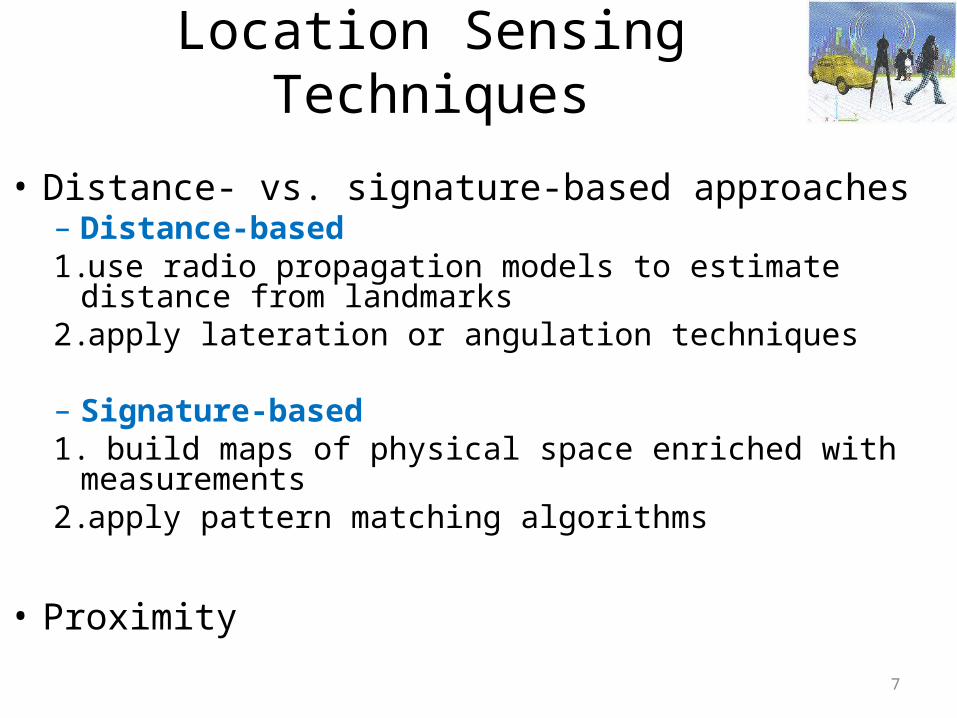
Location Sensing Techniques
• Distance- vs. signature-based approaches– Distance-based1.use radio propagation models to estimate distance from
landmarks2.apply lateration or angulation techniques
– Signature-based1. build maps of physical space enriched with measurements2.apply pattern matching algorithms
• Proximity7

Lateration
8

Angulation
9
• The angle between two nodes can be determined by estimating the AOA parameter of a signal traveling between two nodes
Phased antenna array can be employed

Phased Antenna Array
• Multiple antennas with known separation • Each measures time of arrival of signal• Given the difference in time of arrival & geometry of the receiving
array, the angle from which the emission was originated can be computed• If there are enough elements in the array with large separation, the angulation can be performed
10

Triangulation - Lateration
• Uses geometric properties of triangles to compute object locations• Lateration: Measures distance from reference points
– 2-D requires 3 non-colinear points– 3-D requires 4 non-coplanar points
11

Triangulation - Lateration
Types of Measurements– Direct touch, pressure– Time-of-flight
(e.g., sound waves travel 344m/s in 21oC)
– Signal attenuation• calculate based on send and receive strength• attenuation varies based on environment
12

Time-of-Arrival Issues
• Requires known velocity• May require high time resolution (e.g., for light or radio)
A light pulse (with 299,792,458m/s) will travel the 5m in 16.7ns
Time of flight of light or radio requires clocks with much higher resolution (by 6 orders of magnitude) than those used for timing ultrasound
• Clock synchronization – Possible solution ?
13

Some Real-life Measurements
14

Signal Power Decay with Distance
• A signal traveling from one node to another experiences fast (multipath) fading, shadowing & path loss
• Ideally, averaging RSS over sufficiently long time interval excludes the effects of multipath fading & shadowing general path-loss model:
P(d) = P0 – 10n log10 (d/do)
n: path loss exponent P(d): the average received power in dB at distance d P0 is the received power in dB at a short distance d0
15
_
_

GPS
• 27 satellites • The orbit altitude is such that the satellites repeat the same track and
configuration over any point approximately each 24 hours • Powered by solar energy (also have backup batteries on board)• GPS is a line-of-sight technology the receiver needs a clear view of the satellites it is using to calculate its position • Each satellite has 4 rubidium atomic clocks
– locally averaged to maintain accuracy – updated daily by a Master Control facility
• Satellites are precisely synchronized with each other• Receiver is not synchronized with the satellite transmitter• Satellites transmit their local time in the signal
17

Satellites Orbits
18

Satellites Positions and Orbits
19

GPS (cont’d)• Master Control facility monitors the satellites• Computes
– precise orbital data (i.e., ephemeris) – clock corrections for each satellite
20

GPS Receiver
• Composed of an antenna and preamplifier, radio signal microprocessor, control and display device, data recording unit, & power supply
• Decodes the timing signals from the 'visible' satellites (four or more) • Calculates their distances, its own latitude, longitude, elevation, &
time• A continuous process: the position is updated on a sec-by-sec basis,
output to the receiver display device and, if the receiver provides data capture capabilities, stored by the receiver-logging unit
21

GPS Satellite Signals As light moves through a given medium, low-frequency signals get “refracted”
or slowed more than high-frequency signals
Satellites transmit two microwave carrier signals:• On L1 frequency (1575.42 MHz) it carries the navigation message (satellite orbits, clock corrections & other
system parameters) & a unique identifier code• On L2 frequency (1227.60 MHz) it uses to measure the ionospheric delay By comparing the delays of the two different carrier frequencies of the GPS
signal L1 & L2, we can deduce what the medium is
22

GPS (cont’d)
• Receivers compute their difference in time-of-arrival• Receivers estimate their position (longitude, latitude, elevation) using 4
satellites• 1-5m (95-99%)
23

GPS Error Sources• Noise• Satellites clock errors uncorrected by the controller (~1m)• Ephemeris data errors (~1m)• Troposphere delays due to weather changes e.g., temperature, pressure, humidity (~1m) Troposphere: lower part of the atmosphere, ground level to from 8-13km• Ionosphere delays (~10m) Ionosphere: layer of the atmosphere that consists of ionized air (50-500km)• Multipath (~0.5m)
– caused by reflected signals from surfaces near the receiver that can either interfere with or be mistaken for the signal that follows the straight line path from the satellite
– difficult to be detected and sometime hard to be avoided
24

GPS Error Sources (cont’d)• Control segment mistakes due to computer or human error (1m-100s
km)• Receiver errors from software or hardware failures• User mistakes e.g., incorrect geodetic datum selection (1-100m)
25

Differential GPS (DGPS)• Assumes: any two receivers that are relatively close together
will experience similar atmospheric errors
• Requires reference station: a GPS receiver been set up on a precisely known location
Reference stations calculatetheir position based on satellite signals and compares this location to the known location
26

Differential GPS (cont’d)
• The difference is applied to GPS data recorded by the roving receiver in real time in the field using radio signals or through postprocessing after data capture using special processing software
27

Real-time DGPS
• Reference station calculates & broadcasts corrections for each satellite as it receives the data
• The correction is received by the roving receiver via a radio signal if the source is land based or via a satellite signal if it is satellite based and applied to the position it is calculating
28

Triangulation - Angulation
• 2D requires: 2 angles and 1 known distance
• Phased antenna arrays
29
0°
Angle 1Angle 2
Known Length

Fingerprinting• Create maps of physical space, in which each cell is associated with a
signature (pattern)• A signature of a cell can be build using specific properties of signal
strength measurements collected at that cell• During training, compute the signature @ each position (cell) of the
map (training signature)• At run time, create a signature @ unknown position (cell), using the
same approach as during training for a known cell (runtime signature)• Compare this (runtime) signature, with all (training) signatures, for
each cell of the space, formed during training The cell with a training signature that matches better the runtime
signature is reported as the position of the device
30

Fingerprint
• A fingerprint can be built using various statistical properties– Mean, standard deviation– Percentiles– Empirical distribution (entire set of signal strength values)– Theoretical models (e.g., multivariate Gaussian)
• Fingerprint comparison depends on the statistical properties of the fingerprint Examples:– Euclidean distances, Kullback-Leibler Divergence test
31

Example of a Fingerprint
32

Performance Analysis of Fingerprinting
• Impact of various parameters• Number of APs & other reference points• Size of training set (e.g., number of measurements)• Knowledge of the environment (e.g., floorplan, user
mobility)
33

Empirical Results

Impact of the Number of APs

Collaborative Location Sensing (CLS)
• Each host– estimates its distance from neighboring peers– refines its estimations iteratively as it receives new
positioning information from peers
• Voting algorithm to accumulate and assesses the received positioning information
• Grid-representation of the terrain

Example of voting process @ host u
Host A positioned at the center of the co-centric disks
Host D votes (positive vote)
Most likely position
x
x
Host u with unknown positionPeers A, B, C, and D have positioned themselves
Host A(positive vote)
positive votes from peers A, B, Dnegative vote from peer C Host B votes (positive vote)
x
Host C (negative vote)
x

Example of grid with accumulated votes
The value of a cell in the grid is the sum of the accumulated votesThe higher the value, the more hosts it is likely position of the host
Grid for host uCorresponds to the terrain
Host u tries to position itself
A cell is a possible position
Peers A, B, C
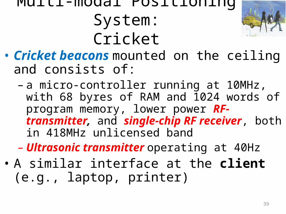
Multi-modal Positioning System:Cricket
• Cricket beacons mounted on the ceiling and consists of:– a micro-controller running at 10MHz, with 68 byres of
RAM and 1024 words of program memory, lower power RF-transmitter, and single-chip RF receiver, both in 418MHz unlicensed band
– Ultrasonic transmitter operating at 40Hz• A similar interface at the client (e.g., laptop,
printer)
39

Cricket Approach
• A cricket beacon sends concurrently an RF message (with info about the space) & an ultrasonic pulse
When the listener @ a client hears the RF signal, it performs the following:– uses the first few bits as training information – turns on its ultrasonic receiver– listens for the ultrasonic pulse which will usually arrive a short time later
1. correlates the RF signal & ultrasonic pulse2. determines the distance to the beacon from the time difference between the receipt of the first bit RF
information & the ultrasonic pulse
40

Cricket Problems
• Lack of coordination can cause:– RF transmissions from different cricket beacons to collide– A listener may correlate incorrectly the RF data of one beacon
with the ultrasonic signal of another, yielding false results• Ultrasonic reception suffers from severe multi-path effect • Order of magnitude longer in time than RF multi-path because of the
relatively long propagation time of sound waves in air
41

Cricket solution
• Handle the problem of collisions using randomization: beacon transmission times are chosen randomly with a uniform distribution within an interval
the broadcasts of different beacons are statistically independent, which avoids repeated synchronization & persistent collisions
Statistical analysis of correlated RF, US samples
42

Proximity
• Physical contact e.g., with pressure, touch sensors or capacitive detectors• Within range of an access point• Automatic ID systems
– computer login– credit card sale– RFID– UPC product codes
43

Sensor Fusion
• Seeks to improve accuracy and precision by aggregating many location-sensing systems (modalities/sources)
to form hierarchical & overlapping levels of resolution• Robustness when a certain location-sensing system (source)
becomes unavailable
Issue: assign weight/importance to the different location-sensing systems
44
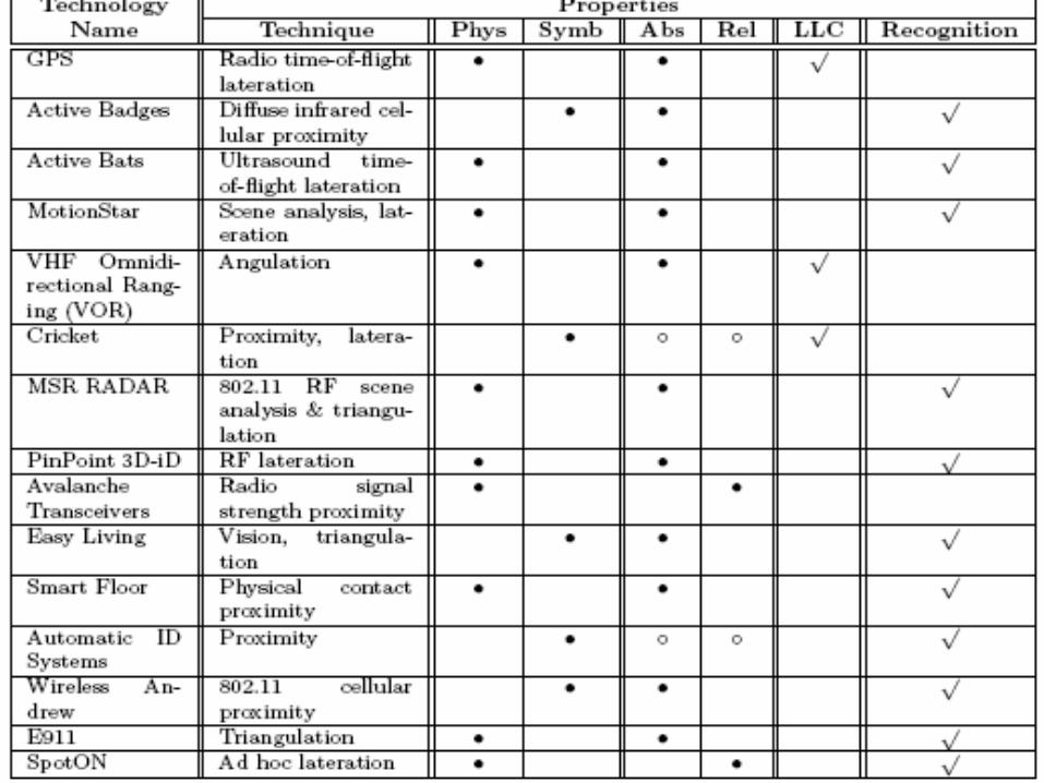
Existing Location Systems
45

Backup Slides
46

Signal-Strength
Left plot: Busy period , Right plot: Quiet period (TNL’s AP)

Multivariate Gaussian Model
• Fingerprint using signal-strength measurements from each AP and the interplay (covariance) of measurements from pairs of Aps
• Signature comparison is based on the Kullback-Leibler Divergence

Multivariate Gaussian Model
• Each cell corresponds to a Multivariate Gaussian distribution
• Measure the similarity of the Multivariate Gaussian distributions (MvGs) with the KLD closed form:

Cretaquarium

Empirical Results (Busy Period)

Empirical Results (Quiet Period)

Impact of the Number of APs
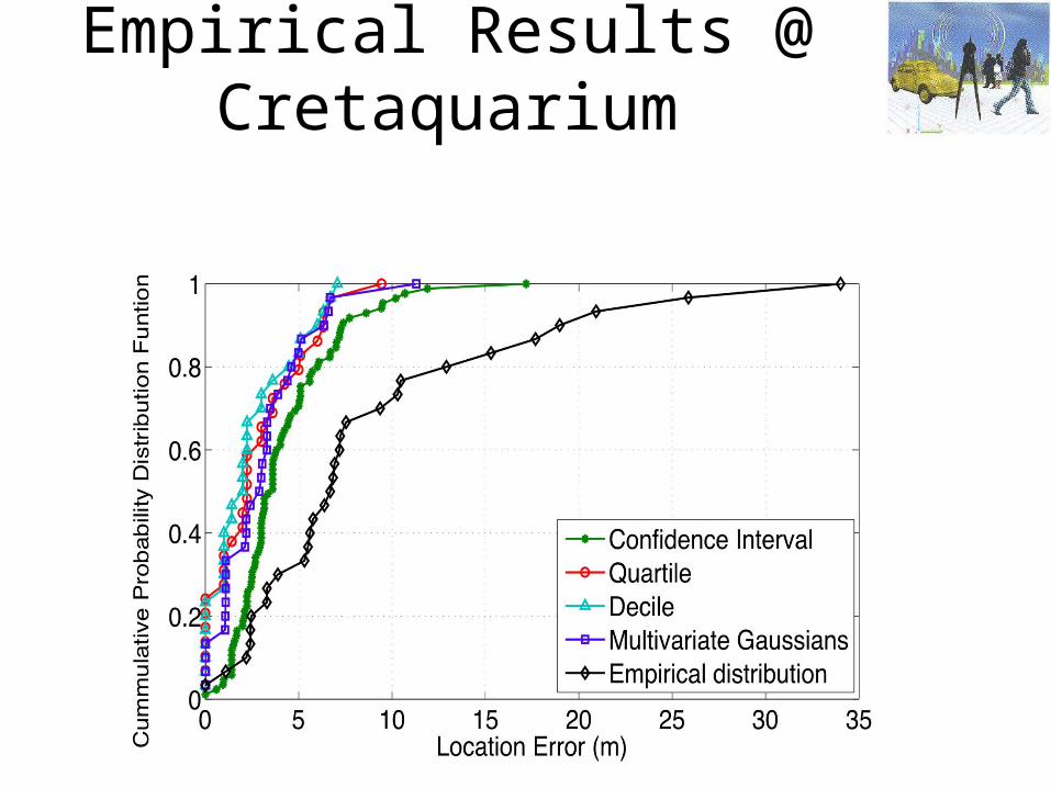
Empirical Results @ Cretaquarium

Collaborative Location Sensing (CLS)
• Each host– estimates its distance from neighboring peers– refines its estimations iteratively as it receives new
positioning information from peers
• Voting algorithm to accumulate and assesses the received positioning information
• Grid-representation of the terrain

Example of voting process @ host u
Host A positioned at the center of the co-centric disks
Host D votes (positive vote)
Most likely position
x
x
Host u with unknown positionPeers A, B, C, and D have positioned themselves
Host A(positive vote)
positive votes from peers A, B, Dnegative vote from peer C Host B votes (positive vote)
x
Host C (negative vote)
x

Example of grid with accumulated votes
The value of a cell in the grid is the sum of the accumulated votesThe higher the value, the more hosts it is likely position of the host
Grid for host uCorresponds to the terrain
Host u tries to position itself
A cell is a possible position
Peers A, B, C

Signal-Strength
Left plot: Busy period , Right plot: Quiet period (TNL’s AP)

Multivariate Gaussian Model
• Fingerprint using signal-strength measurements from each AP and the interplay (covariance) of measurements from pairs of Aps
• Signature comparison is based on the Kullback-Leibler Divergence

Multivariate Gaussian Model
• Each cell corresponds to a Multivariate Gaussian distribution
• Measure the similarity of the Multivariate Gaussian distributions (MvGs) with the KLD closed form:

Cretaquarium

Empirical Results @ Cretaquarium

Empirical Results (Busy Period)

Experimental Results – Quiet Period (%)

Splitting into areas of cells - TNL (1/2)• Split the grid in 14 regions, namely from A to N
– The regions are overlapped– Collect the data from each cell that belongs in this region– Concat them in a new file named Region{A to N}– 16 APs average in
every region

Splitting into areas of cells - TNL (2/2)

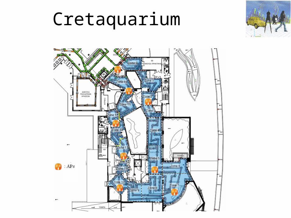
Testbed description - Aquarium
– 1760 m^2– 30 tanks (extra 25 will be installed)– 8 APs– Cell’s size: 1m x 1m– 5.7 APs on average were collected– About 150 visitors

Test bed description - TNL
– 7 x 12 m– Cell’s size: 55 x 55 cm– 13 APs– 6 APs average detected
at a cell
108 training cells30 run-time cells

Experimental Results
• Two real map databases obtained from TNL– Busy period data – Quiet period data
• Real database obtained from Cretaquarium (Normal period data)
• Performance of positioning in terms of localization error.
• Measured by averaging the Euclidean distance between the estimated location of the mobile user and its true location

Signal-Strength
Left plot: Busy period , Right plot: Quiet period (TNL’s AP)

Multivariate Gaussian Model
• Fingerprint using signal-strength measurements from each AP and the interplay (covariance) of measurements from pairs of Aps
• Signature comparison is based on the Kullback-Leibler Divergence

Multivariate Gaussian Model
• Each cell corresponds to a Multivariate Gaussian distribution
• Measure the similarity of the Multivariate Gaussian distributions (MvGs) with the KLD closed form:
Cretaquarium

Empirical Results @ Cretaquarium

Empirical Results (Quiet Period)