Embed Size (px)
Citation preview

1
Pertemuan 11Sampling dan Sebaran Sampling-1
Matakuliah : A0064 / Statistik Ekonomi
Tahun : 2005
Versi : 1/1

2
Learning Outcomes
Pada akhir pertemuan ini, diharapkan mahasiswa
akan mampu :• Menjelaskan pengertian dan tujuan sampling,
serta dapat memberikan contoh tentang sampel statistik dan parameter populasi

3
Outline Materi
• Sampel Statistik sebagai Estimator bagi Parameter Populasi
• Sebaran Sampling

COMPLETE 5 t h e d i t i o nBUSINESS STATISTICS
Aczel/SounderpandianMcGraw-Hill/Irwin © The McGraw-Hill Companies, Inc.,2002
5-4
Using Statistics Sample Statistics as Estimators of
Population Parameters Sampling Distributions Estimators and Their Properties Degrees of Freedom Using the Computer Summary and Review of Terms
Sampling and Sampling Distributions5

COMPLETE 5 t h e d i t i o nBUSINESS STATISTICS
Aczel/SounderpandianMcGraw-Hill/Irwin © The McGraw-Hill Companies, Inc.,2002
5-5
• Statistical Inference: Predict and forecast values of
population parameters... Test hypotheses about values
of population parameters... Make decisions...
On basis of sample statistics derived from limited and incomplete sample information
Make generalizations about the characteristics of a population...
Make generalizations about the characteristics of a population...
On the basis of observations of a sample, a part of a population
On the basis of observations of a sample, a part of a population
5-1 Statistics is a Science of InferenceInference
COMPLETE 5 t h e d i t i o nBUSINESS STATISTICS
Aczel/SounderpandianMcGraw-Hill/Irwin © The McGraw-Hill Companies, Inc.,2002
5-6
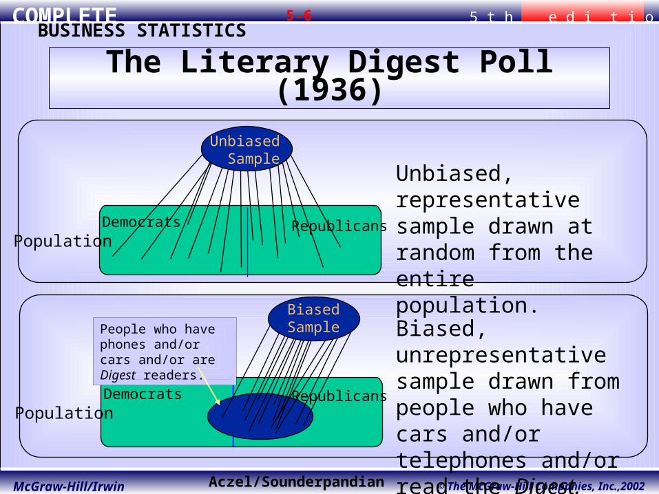
Democrats Republicans
People who have phones and/or cars and/or are Digest readers.
BiasedSample
Population
Democrats Republicans
Unbiased Sample
Population
Unbiased, representative sample drawn at random from the entire population.
Biased, unrepresentative sample drawn from people who have cars and/or telephones and/or read the Digest.
The Literary Digest Poll (1936)

COMPLETE 5 t h e d i t i o nBUSINESS STATISTICS
Aczel/SounderpandianMcGraw-Hill/Irwin © The McGraw-Hill Companies, Inc.,2002
5-7
• An estimatorestimator of a population parameter is a sample statistic used to estimate or predict the population parameter.
• An estimateestimate of a parameter is a particular numerical value of a sample statistic obtained through sampling.
• A point estimatepoint estimate is a single value used as an estimate of a population parameter.
A population parameterpopulation parameter is a numerical measure of a summary characteristic of a population.
5-2 Sample Statistics as Estimators of Population Parameters
• A sample statisticsample statistic is a numerical measure of a summary characteristic
of a sample.

COMPLETE 5 t h e d i t i o nBUSINESS STATISTICS
Aczel/SounderpandianMcGraw-Hill/Irwin © The McGraw-Hill Companies, Inc.,2002
5-8
• The sample mean, , is the most common estimator of the population mean,
• The sample variance, s2, is the most common estimator of the population variance, 2.
• The sample standard deviation, s, is the most common estimator of the population standard deviation, .
• The sample proportion, , is the most common estimator of the population proportion, p.
Estimators
X
p̂

COMPLETE 5 t h e d i t i o nBUSINESS STATISTICS
Aczel/SounderpandianMcGraw-Hill/Irwin © The McGraw-Hill Companies, Inc.,2002
5-9
• The population proportionpopulation proportion is equal to the number of elements in the population belonging to the category of interest, divided by the total number of elements in the population:
• The sample proportionsample proportion is the number of elements in the sample belonging to the category of interest, divided by the sample size:
Population and Sample Proportions
pxn
pXN

COMPLETE 5 t h e d i t i o nBUSINESS STATISTICS
Aczel/SounderpandianMcGraw-Hill/Irwin © The McGraw-Hill Companies, Inc.,2002
5-10
XX
XXX
XX
XXX
XXX
XXX
XX
Population mean ()
Sample points
Frequency distribution of the population
Sample mean ( )
A Population Distribution, a Sample from a Population, and the Population and Sample Means
X

COMPLETE 5 t h e d i t i o nBUSINESS STATISTICS
Aczel/SounderpandianMcGraw-Hill/Irwin © The McGraw-Hill Companies, Inc.,2002
5-11
• The sampling distributionsampling distribution of a statistic is the probability distribution of all possible values the statistic may assume, when computed from random samples of the same size, drawn from a specified population.
• The sampling distribution of sampling distribution of XX is the probability distribution of all possible values the random variable may assume when a sample of size n is taken from a specified population.
X
5-3 Sampling Distributions

COMPLETE 5 t h e d i t i o nBUSINESS STATISTICS
Aczel/SounderpandianMcGraw-Hill/Irwin © The McGraw-Hill Companies, Inc.,2002
5-12
Uniform population of integers from 1 to 8:
X P(X) XP(X) (X-x) (X-x)2 P(X)(X-x)2
1 0.125 0.125 -3.5 12.25 1.531252 0.125 0.250 -2.5 6.25 0.781253 0.125 0.375 -1.5 2.25 0.281254 0.125 0.500 -0.5 0.25 0.031255 0.125 0.625 0.5 0.25 0.031256 0.125 0.750 1.5 2.25 0.281257 0.125 0.875 2.5 6.25 0.781258 0.125 1.000 3.5 12.25 1.53125
1.000 4.500 5.25000 87654321
0.2
0.1
0.0
X
P(X
)
Uniform Distribution (1,8)
E(X) = E(X) = = 4.5 = 4.5V(X) = V(X) = 22 = 5.25 = 5.25SD(X) = SD(X) = = 2.2913 = 2.2913
Sampling Distributions (Continued)

COMPLETE 5 t h e d i t i o nBUSINESS STATISTICS
Aczel/SounderpandianMcGraw-Hill/Irwin © The McGraw-Hill Companies, Inc.,2002
5-13
• There are 8*8 = 64 different but equally-likely samples of size 2 that can be drawn (with replacement) from a uniform population of the integers from 1 to 8:Samples of Size 2 from Uniform (1,8)
1 2 3 4 5 6 7 81 1,1 1,2 1,3 1,4 1,5 1,6 1,7 1,82 2,1 2,2 2,3 2,4 2,5 2,6 2,7 2,83 3,1 3,2 3,3 3,4 3,5 3,6 3,7 3,84 4,1 4,2 4,3 4,4 4,5 4,6 4,7 4,85 5,1 5,2 5,3 5,4 5,5 5,6 5,7 5,86 6,1 6,2 6,3 6,4 6,5 6,6 6,7 6,87 7,1 7,2 7,3 7,4 7,5 7,6 7,7 7,88 8,1 8,2 8,3 8,4 8,5 8,6 8,7 8,8
Each of these samples has a sample mean. For example, the mean of the sample (1,4) is 2.5, and the mean of the sample (8,4) is 6.
Sample Means from Uniform (1,8), n = 21 2 3 4 5 6 7 8
1 1.0 1.5 2.0 2.5 3.0 3.5 4.0 4.52 1.5 2.0 2.5 3.0 3.5 4.0 4.5 5.03 2.0 2.5 3.0 3.5 4.0 4.5 5.0 5.54 2.5 3.0 3.5 4.0 4.5 5.0 5.5 6.05 3.0 3.5 4.0 4.5 5.0 5.5 6.0 6.56 3.5 4.0 4.5 5.0 5.5 6.0 6.5 7.07 4.0 4.5 5.0 5.5 6.0 6.5 7.0 7.58 4.5 5.0 5.5 6.0 6.5 7.0 7.5 8.0
Sampling Distributions (Continued)

COMPLETE 5 t h e d i t i o nBUSINESS STATISTICS
Aczel/SounderpandianMcGraw-Hill/Irwin © The McGraw-Hill Companies, Inc.,2002
5-14
Sampling Distribution of the Mean
The probability distribution of the sample mean is called the sampling distribution of the the sample meansampling distribution of the the sample mean.
8.07.57.06.56.05.55.04.54.03.53.02.52.01.51.0
0.10
0.05
0.00
X
P(X
)
Sampling Distribution of the Mean
X P(X) XP(X) X-X (X-X)2 P(X)(X-X)2
1.0 0.015625 0.015625 -3.5 12.25 0.1914061.5 0.031250 0.046875 -3.0 9.00 0.2812502.0 0.046875 0.093750 -2.5 6.25 0.2929692.5 0.062500 0.156250 -2.0 4.00 0.2500003.0 0.078125 0.234375 -1.5 2.25 0.1757813.5 0.093750 0.328125 -1.0 1.00 0.0937504.0 0.109375 0.437500 -0.5 0.25 0.0273444.5 0.125000 0.562500 0.0 0.00 0.0000005.0 0.109375 0.546875 0.5 0.25 0.0273445.5 0.093750 0.515625 1.0 1.00 0.0937506.0 0.078125 0.468750 1.5 2.25 0.1757816.5 0.062500 0.406250 2.0 4.00 0.2500007.0 0.046875 0.328125 2.5 6.25 0.2929697.5 0.031250 0.234375 3.0 9.00 0.2812508.0 0.015625 0.125000 3.5 12.25 0.191406
1.000000 4.500000 2.625000
E XV XSD X
X
X
X
( )( )
( ) .
4.52.62516202
2
Sampling Distributions (Continued)

COMPLETE 5 t h e d i t i o nBUSINESS STATISTICS
Aczel/SounderpandianMcGraw-Hill/Irwin © The McGraw-Hill Companies, Inc.,2002
5-15
• Comparing the population distribution and the sampling distribution of the mean:The sampling distribution is
more bell-shaped and symmetric.
Both have the same center.The sampling distribution of
the mean is more compact, with a smaller variance.
87654321
0.2
0.1
0.0
X
P(X
)
Uniform Distribution (1,8)
X8.07.57.06.56.05.55.04.54.03.53.02.52.01.51.0
0.10
0.05
0.00
P( X
)
Sampling Distribution of the Mean
Properties of the Sampling Distribution of the Sample Mean

COMPLETE 5 t h e d i t i o nBUSINESS STATISTICS
Aczel/SounderpandianMcGraw-Hill/Irwin © The McGraw-Hill Companies, Inc.,2002
5-16
The expected value of the sample meanexpected value of the sample mean is equal to the population mean:
E XX X
( )
The variance of the sample meanvariance of the sample mean is equal to the population variance divided by the sample size:
V XnX
X( ) 2
2
The standard deviation of the sample mean, known as the standard error of standard deviation of the sample mean, known as the standard error of the meanthe mean, is equal to the population standard deviation divided by the square root of the sample size:
SD XnX
X( )
Relationships between Population Parameters and the Sampling Distribution of the Sample Mean

COMPLETE 5 t h e d i t i o nBUSINESS STATISTICS
Aczel/SounderpandianMcGraw-Hill/Irwin © The McGraw-Hill Companies, Inc.,2002
5-17
When sampling from a normal populationnormal population with mean and standard deviation , the sample mean, X, has a normal sampling distributionnormal sampling distribution:
When sampling from a normal populationnormal population with mean and standard deviation , the sample mean, X, has a normal sampling distributionnormal sampling distribution:
X Nn
~ ( , ) 2
This means that, as the sample size increases, the sampling distribution of the sample mean remains centered on the population mean, but becomes more compactly distributed around that population mean
This means that, as the sample size increases, the sampling distribution of the sample mean remains centered on the population mean, but becomes more compactly distributed around that population mean
Normal population
0.4
0.3
0.2
0.1
0.0
f (X)
Sampling Distribution of the Sample Mean
Sampling Distribution: n =2
Sampling Distribution: n =16
Sampling Distribution: n =4
Sampling from a Normal Population
Normal population

COMPLETE 5 t h e d i t i o nBUSINESS STATISTICS
Aczel/SounderpandianMcGraw-Hill/Irwin © The McGraw-Hill Companies, Inc.,2002
5-18
When sampling from a population with mean and finite standard deviation , the sampling distribution of the sample mean will tend to a normal distribution with mean and standard deviation as the sample size becomes large(n >30).
For “large enough” n:
When sampling from a population with mean and finite standard deviation , the sampling distribution of the sample mean will tend to a normal distribution with mean and standard deviation as the sample size becomes large(n >30).
For “large enough” n:
n
)/,(~ 2 nNX
P( X)
X
0.25
0.20
0.15
0.10
0.05
0.00
n = 5
P( X)
0.2
0.1
0.0 X
n = 20
f ( X)
X
-
0.4
0.3
0.2
0.1
0.0
Large n
The Central Limit Theorem

COMPLETE 5 t h e d i t i o nBUSINESS STATISTICS
Aczel/SounderpandianMcGraw-Hill/Irwin © The McGraw-Hill Companies, Inc.,2002
5-19
Normal Uniform Skewed
Population
n = 2
n = 30
XXXX
General
The Central Limit Theorem Applies to Sampling Distributions from AnyAny Population
COMPLETE 5 t h e d i t i o nBUSINESS STATISTICS
Aczel/SounderpandianMcGraw-Hill/Irwin © The McGraw-Hill Companies, Inc.,2002
5-20
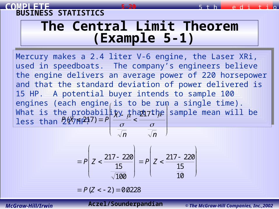
Mercury makes a 2.4 liter V-6 engine, the Laser XRi, used in speedboats. The company’s engineers believe the engine delivers an average power of 220 horsepower and that the standard deviation of power delivered is 15 HP. A potential buyer intends to sample 100 engines (each engine is to be run a single time). What is the probability that the sample mean will be less than 217HP?
Mercury makes a 2.4 liter V-6 engine, the Laser XRi, used in speedboats. The company’s engineers believe the engine delivers an average power of 220 horsepower and that the standard deviation of power delivered is 15 HP. A potential buyer intends to sample 100 engines (each engine is to be run a single time). What is the probability that the sample mean will be less than 217HP?
P X PX
n n
P Z P Z
P Z
( )
( ) .
217217
217 22015
100
217 2201510
2 0 0228
The Central Limit Theorem (Example 5-1)

COMPLETE 5 t h e d i t i o nBUSINESS STATISTICS
Aczel/SounderpandianMcGraw-Hill/Irwin © The McGraw-Hill Companies, Inc.,2002
5-21
Example 5-2
EPS Mean Distribution
0
5
10
15
20
25
Range
Fre
qu
en
cy
2.00 - 2.49
2.50 - 2.99
3.00 - 3.49
3.50 - 3.99
4.00 - 4.49
4.50 - 4.99
5.00 - 5.49
5.50 - 5.99
6.00 - 6.49
6.50 - 6.99
7.00 - 7.49
7.50 - 7.99

COMPLETE 5 t h e d i t i o nBUSINESS STATISTICS
Aczel/SounderpandianMcGraw-Hill/Irwin © The McGraw-Hill Companies, Inc.,2002
5-22
If the population standard deviation, , is unknownunknown, replace with the sample standard deviation, s. If the population is normal, the resulting statistic: has a t distribution t distribution with with (n - 1) degrees of freedom(n - 1) degrees of freedom.
If the population standard deviation, , is unknownunknown, replace with the sample standard deviation, s. If the population is normal, the resulting statistic: has a t distribution t distribution with with (n - 1) degrees of freedom(n - 1) degrees of freedom.• The t is a family of bell-shaped and symmetric
distributions, one for each number of degree of freedom.
• The expected value of t is 0.
• The variance of t is greater than 1, but approaches 1 as the number of degrees of freedom increases. The t is flatter and has fatter tails than does the standard normal.
• The t distribution approaches a standard normal as the number of degrees of freedom increases.
• The t is a family of bell-shaped and symmetric distributions, one for each number of degree of freedom.
• The expected value of t is 0.
• The variance of t is greater than 1, but approaches 1 as the number of degrees of freedom increases. The t is flatter and has fatter tails than does the standard normal.
• The t distribution approaches a standard normal as the number of degrees of freedom increases.
nsXt
/
Standard normal
t, df=20t, df=10
Student’s t Distribution

COMPLETE 5 t h e d i t i o nBUSINESS STATISTICS
Aczel/SounderpandianMcGraw-Hill/Irwin © The McGraw-Hill Companies, Inc.,2002
5-23
The sample proportionsample proportion is the percentage of successes in n binomial trials. It is the number of successes, X, divided by the number of trials, n.
The sample proportionsample proportion is the percentage of successes in n binomial trials. It is the number of successes, X, divided by the number of trials, n.
pX
n
As the sample size, n, increases, the sampling distribution of approaches a normal normal distributiondistribution with mean p and standard deviation
As the sample size, n, increases, the sampling distribution of approaches a normal normal distributiondistribution with mean p and standard deviation
p
p pn
( )1
Sample proportion:
1514131211109876543210
0.2
0.1
0.0
P(X)
n=15, p = 0.3
X
1415
1315
1215
1115
10 15
9 15
8 15
7 15
6 15
5 15
4 15
3 15
2 15
1 15
0 15
1515 ^
p
210
0 .5
0 .4
0 .3
0 .2
0 .1
0 .0
X
P(X)
n=2, p = 0.3
109876543210
0.3
0.2
0.1
0.0
P(X
)
n=10,p=0.3
X
The Sampling Distribution of the Sample Proportion, p

COMPLETE 5 t h e d i t i o nBUSINESS STATISTICS
Aczel/SounderpandianMcGraw-Hill/Irwin © The McGraw-Hill Companies, Inc.,2002
5-24
In recent years, convertible sports coupes have become very popular in Japan. Toyota is currently shipping Celicas to Los Angeles, where a customizer does a roof lift and ships them back to Japan. Suppose that 25% of all Japanese in a given income and lifestyle category are interested in buying Celica convertibles. A random sample of 100 Japanese consumers in the category of interest is to be selected. What is the probability that at least 20% of those in the sample will express an interest in a Celica convertible?
In recent years, convertible sports coupes have become very popular in Japan. Toyota is currently shipping Celicas to Los Angeles, where a customizer does a roof lift and ships them back to Japan. Suppose that 25% of all Japanese in a given income and lifestyle category are interested in buying Celica convertibles. A random sample of 100 Japanese consumers in the category of interest is to be selected. What is the probability that at least 20% of those in the sample will express an interest in a Celica convertible?
n
p
np E p
p p
nV p
p p
nSD p
100
0 25
100 0 25 25
1 25 75
1000 001875
10 001875 0 04330127
.
( )( . ) ( )
( ) (. )(. ). ( )
( ). . ( )
P p Pp p
p p
n
p
p p
n
P z P z
P z
( . )
( )
.
( )
. .
(. )(. )
.
.
( . ) .
0 201
20
1
20 25
25 75
100
05
0433
1 15 0 8749
Sample Proportion (Example 5-3)

25
Penutup
• Pembahasan materi dilanjutkan dengan Materi Pokok 12 (Sampling dan Sebaran Sampling-2)


![RM Presentation Sampling & Non Sampling Error[1]](https://img.pdfslide.net/doc/110x75/577ce47b1a28abf1038e72fc/rm-presentation-sampling-non-sampling-error1.jpg)