Embed Size (px)
Citation preview
Topic 1 --- page 1
Topic 1: Sampling and Sampling Distributions
Chapter 7
Objective: To draw inferences about population
parameters on the basis of sample information.
In Economics 245 (Descriptive Statistics) we saw that statistics are
largely applied to describing ______________parameters, and
estimating or testing hypotheses about population characteristics.
Example: measures of central tendency, such as the population
mean, median, and mode;
measures of d , such as the population
variance, standard deviation, coefficient of
variation.
Topic 1 --- page 2
If all values of a ___________ are known, we can determine
these parameters.
But for many populations, there are monetary and ____constraints
to the act of gathering data from an entire population to determine
the population parameter of interest.
Hence, _______are taken to estimate the population parameters.
In Topic 1 we will explore how a sample is taken, and how
the information generated from the sample can be applied.

Topic 1 --- page 3
Topic 1 --- page 4
Topic 1 --- page 5

Topic 1 --- page 6
Topic 1 --- page 7
To deal with the issues of proper sampling, we must ask the
following questions:
1) What are the most ____ efficient means of collecting
samples that generate the best representation of the
population?
2) How do we clearly describe s_____information in the
most useful manner?
3) How do we generate inferences about the population from
______ summaries?
4) How accurate are the inferences generated from _____
information?

Topic 1 --- page 8
Sample Design
To answer question #1, we must describe how _____ data is
collected. (i.e. describe the procedure or plan of action.)
Definition:
Sample Design: is a pre-determined ____ depicting how to collect
a sample from a given population.
That is, before any data collection takes place, the researcher
_____ how he or she will actually collect the data.
The primary objective of the sample design is to collect a ______
that accurately resembles the population that one is trying to
replicate by a ________.

Topic 1 --- page 9
Ideally, the ______contains population “characteristics” in the
same proportion or concentration.
Ex. Suppose some population contains a 6.5% unemployment rate.
(Obtained from the Census).
The ______ must contain 6.5 % unemployed.
Ex. 50% of the population is over 60 years old.
Want a ______ that has 50% of the people surveyed over
60 years old.
Topic 1 --- page 10
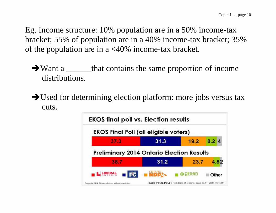
Eg. Income structure: 10% population are in a 50% income-tax
bracket; 55% of population are in a 40% income-tax bracket; 35%
of the population are in a <40% income-tax bracket.
Want a ______that contains the same proportion of income
distributions.
Used for determining election platform: more jobs versus tax
cuts.
Topic 1 --- page 11

Topic 1 --- page 12

Topic 1 --- page 13
There are many ways of collecting a bad _______.
Let us look at some of the errors that can be created from bad
sampling _______:
(I) Non-________ Errors: these are errors that include all different human errors, such
as mistakes in collecting, analysing and reporting data.
Examples:
i) Wrong population is _______: An error of misrepresentation
can arise when the wrong population is sampled by mistake.
i.e. A survey question, when applied to a certain _______,
misrepresents the true population response because the sample did
not accurately replicate the population.

Topic 1 --- page 14
Example: “Should hours of operation for ____ downtown be
extended?” asked to the average person in a bar at 2 a.m. in
downtown Vancouver. The positive or negative _________may be
higher or lower than the Canadian average.

Topic 1 --- page 15
ii) Response ____: Another type of error, know as response ___,
affects results in surveys.
Due to: poor _______ on questionnaires.
Interview techniques that cause the interviewee to respond
to a question that does not reflect his / her true opinion.
Distorts the truth.
Example: Air quality control survey: “Do you drive an automobile
that is environmentally friendly?”
Answer ‘no’ if you do not have a car.
Or perception of your car’s environmental friendliness is
high, but in reality your car would fail every test available, so your
response misrepresents the population.
Your perception may be subjective if the survey does not specify
some criterion.
Topic 1 --- page 16
(II) Sampling _________:
Errors that represent the differences that may ______between a
sample statistic and the population parameter being estimated are
called sampling errors.
Will _______ occur in all data collection except a census where
all items are surveyed.
Occurs in a situation where the sample does not represent the
true population being examined because the sample only represents
a portion of a population.
An inferential error may be made because the data collected
from the _____ does not truly reflect the characteristic of the true
population being explored.

Topic 1 --- page 17
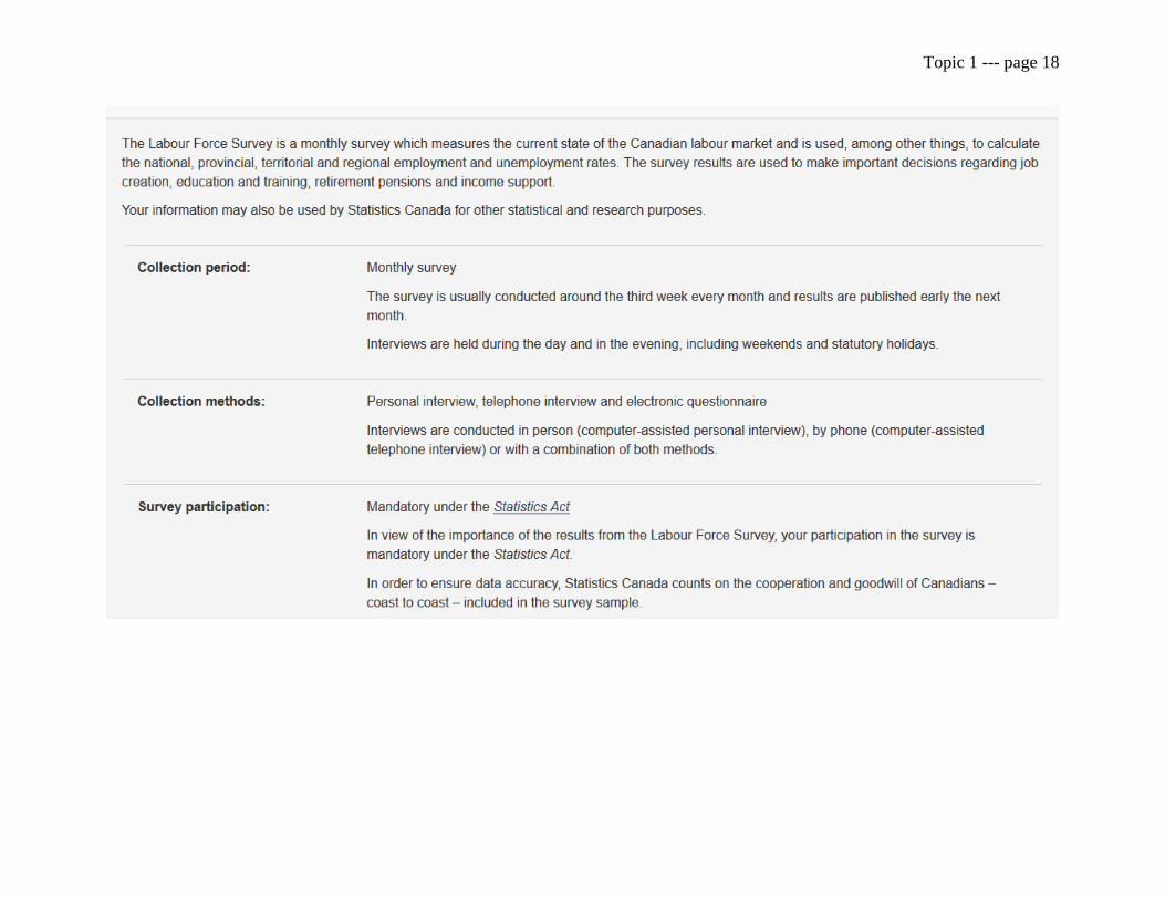
Example: The unemployment rate calculated from the Labour
Force Survey understates the actual unemployment rate because it
excludes certain groups within the provincial level, such as people
on native reserves, people living in the NWT, Yukon and Nunavut.
Topic 1 --- page 18
Topic 1 --- page 19
There is usually a trade-off between ______ design and the
cost of making an ______.
In order to minimize the cost of erroneous decisions based on
inaccurate information, the researcher must improve the
_______ design.
But such improvements are expensive.
“Balance the costs of making an error and cost of
sampling.”
(Not easy – hard to specify the cost of making an incorrect
decision!

Topic 1 --- page 20
Next: Determining Which Sample Designs Most Effectively
Minimize Sampling Errors
I) Sampling
Based on a random selection process.
One criterion for a good _______is that every item in the
population being examined has an equal and independent
chance of being chosen as part of the _______.
A) _______ Random Samples: Every item of a sample of size n (from a population of
size N,) is equally likely to be chosen.
Requirement: access to all items in the population.
Can be difficult if the population is large and elements are
difficult to identify.
Topic 1 --- page 21
B) Systematic S_________:
A random starting point in the population is selected, and
every kth element thereafter is a _____ point in the sample.
Not equivalent to simple random sampling because
every set of n items does not have an equal probability of
being selected.
Bias will result if we have p_______ to the items in the
population.
Example: Want to determine average time in movie line-ups.
Sample the wait times on “cheap night ” Tuesday:
Sampling time on a single day of the week, rather than a daily
pattern, will result in bias amount recorded.
Topic 1 --- page 22
Example: Sleeping: What is the average amount of sleep an
individual achieves each night?
Sample times on Friday night.
Sampling time on a single day of the week,
rather than a daily pattern, will result in bias
amount recorded.

Topic 1 --- page 23
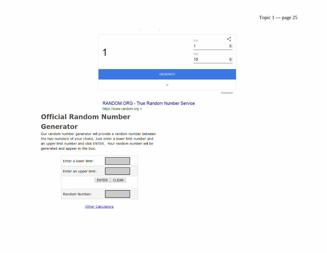
The systematic way of drawing a simple random sample is
to select a sample with the help of a random number
table / generator.
In Random number table, sequence of random integers
between 0 - 9 are generated at random.
Each has the same probability of occurrence.

Topic 1 --- page 24
Topic 1 --- page 25

Topic 1 --- page 26
Topic 1 --- page 27
Example Using EViews:
Random Number Generator in EViews:
(i) Uniform random integer Generator:
The rndint command will create (pseudo) random integers
drawn uniformly from zero to a specifed maximum.
The rndint command ignores the current sample and fills
the entire object with random integers.
Syntax
Command: rndint(object_name, n)
Topic 1 --- page 28
Type the name of the series object to fill followed by an
integer value representing the maximum value n of the
random integers.
n should be a positive integer.
Example: Suppose we want to create a series of 10 random
integers with a value from zero to 100.
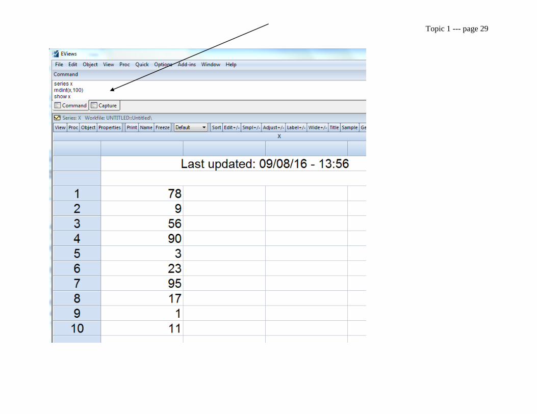
Type in the following code in the command window in a new
workfile (with a range of 10):
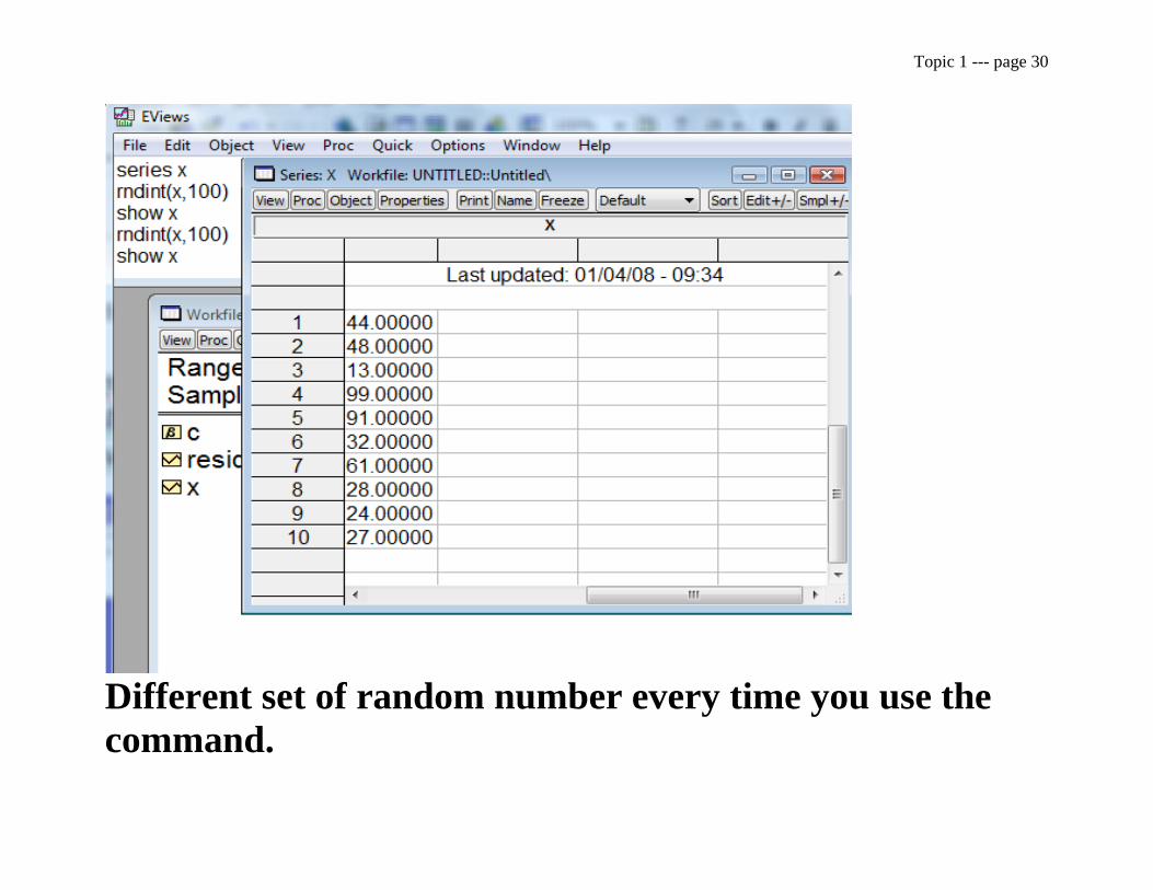
series x
rndint(x,100)
Hit return.
Topic 1 --- page 29
Topic 1 --- page 30
Different set of random number every time you use the
command.
Topic 1 --- page 31
Sampling With _______Knowledge
Simple random ________ may be difficult when the
population is large and certain elements of the population are
hard to identify.
Problems: Expensive
Time consuming
There are two random sampling techniques that use _____
knowledge about the population and hence, reduce the costs
of simple random sampling:
1) Stratified Sampling
2) Cluster Sampling

Topic 1 --- page 32
(I) Sampling
This technique divides the population into a number of
distinct and similar subgroups, and then selects a
proportionate number of items from each subgroup.
“The use of stratified sampling requires that a population be
divided into __________ groups called strata. Each stratum
is then sampled according to certain specified criteria.”
If we can identify certain characteristics in the population
and can separate these characteristics into subgroups, we
require fewer sample points to determine the level or
concentration of the characteristic under study.

Topic 1 --- page 33
The optimal method of selecting strata is to find groups
with a ______variability between strata, but with only a ____
variability within the strata.
i.e. Groups should have large inter-strata variation, but little
intra-strata variation.
Each subgroup contains persons who share common traits
and each subgroup is distinctly different.
Topic 1 --- page 34
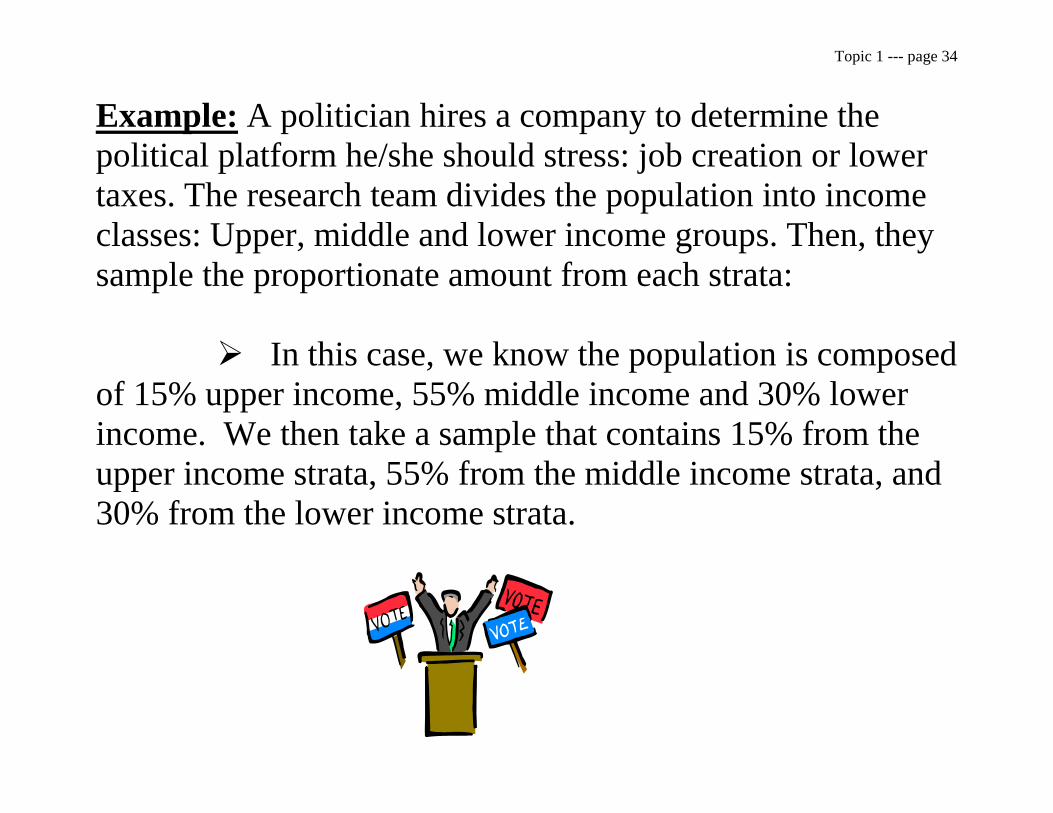
Example: A politician hires a company to determine the
political platform he/she should stress: job creation or lower
taxes. The research team divides the population into income
classes: Upper, middle and lower income groups. Then, they
sample the proportionate amount from each strata:
In this case, we know the population is composed
of 15% upper income, 55% middle income and 30% lower
income. We then take a sample that contains 15% from the
upper income strata, 55% from the middle income strata, and
30% from the lower income strata.
Topic 1 --- page 35
Advantages:
(1) If homogeneous subsets of a population can be identified, then
only a relatively small number of sample observations are needed
to determine the characteristics of each subset. Thus, stratified
sampling is usually less expensive than simple random sampling,
because we only require a small number of sample points to get an
accurate measure of the characteristic under study.
(2) Use of _____ knowledge about the population may improve
the accuracy of the statistical inference based on stratified
sampling as compared to simple random sampling
improvement in the “efficiency” of the estimate.

Topic 1 --- page 36
Example: The cost of post secondary education is higher for
people who do not live in a city with a university. We want to
measure the average size of a student loan.
65% of university students are residents of the city.
35% are from other parts of the province.
If we divide students into two strata: residents and non-residents,
and then sample in the same proportion, we may get a better
average student loan estimate.
65% of university
students are residents
of the city
35% are from other
parts of the province

Topic 1 --- page 37
(3) By-Product: A side-effect
In dividing the population into strata, a valuable side effect
is produced.
Can determine inferences about each group without further
sampling.
Example: Continuation from above: If you wanted to know the
average loan size of students that are not residents of the university
city, we would sample from that group.
Topic 1 --- page 38
Example: Studying the average wage rate in Canada: It is
believed that people in large cities earn higher wages than
people in smaller towns. Could divide the population of
Canada into urban and rural strata. Then, study the wage rate
of each group to get an average wage rate in Canada.
Example: We want to determine if there is a difference
between the average amount of healthcare consumed by the
rich and the poor. The researcher would divide the people into
strata according to their gross incomes. Then the researcher
could sample each stratum to determine if there is a
statistically significant difference between healthcare usage
among the two groups.
Topic 1 --- page 39
(II) ____________Sampling The population is subdivided into groups called clusters,
where each cluster has the same characteristics as the
population.
Each cluster is assumed to be representative of the
_________. Hence, the researcher has only to pick a few
clusters to constitute the ______ in order to estimate the
characteristics of the population.
All elements in each cluster is taken to constitute the
________.
Procedure: 1) Divide the population into clusters.
2) Randomly select a ______ of clusters.
3) Select all the elements in each selected cluster.
Topic 1 --- page 40
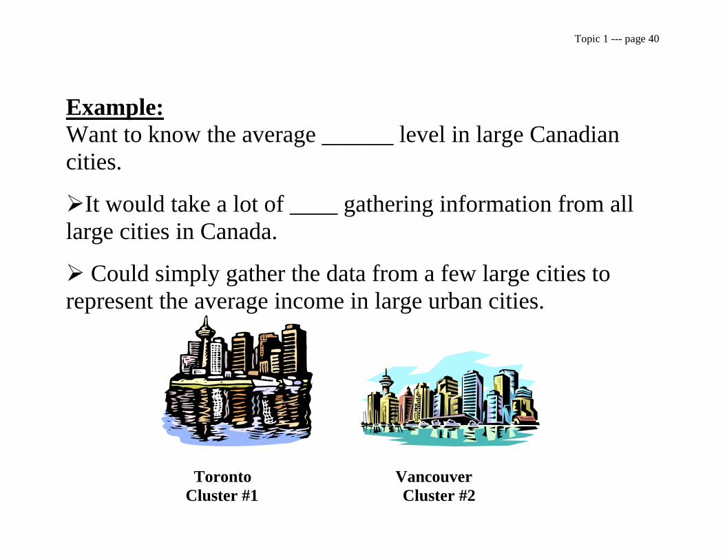
Example:
Want to know the average ______ level in large Canadian
cities.
It would take a lot of ____ gathering information from all
large cities in Canada.
Could simply gather the data from a few large cities to
represent the average income in large urban cities.
Toronto Vancouver
Cluster #1 Cluster #2

Topic 1 --- page 41
Example: The researcher is interested in some student
characteristic. All the ______ in Canada is the population. Form
clusters: Group together all students at all universities: Uvic, UBC,
SFU, York, Guelph, Queens, McGill, etc.,. It would be very costly
to sample all universities, but we could pick a few universities and
look at all of the _______ at those universities to estimate some
population characteristic.
Optimal Way of Selecting Clusters:
Have groups that have a lot of _______-cluster variation, but little
____-cluster variation.
i.e. There should be ______ variation between groups, but a____
variability within each group that represents the population.

Topic 1 --- page 42
Advantages:
1) Lowers the ____ of sampling when the population is large.
2) Better results when do not have a total accounting or full access
to all the _________ about the population in question.
Disadvantage:
1) Clusters may not be truly representative of the population:
Geographical ____.
The student cluster at the University of Northern B.C. may be
different to the typical Vancouver area campus cluster. Because of
the location of the university, there may be large differences in
class size, loan size, family background, average age, political
beliefs, etc.... Or not.
Topic 1 --- page 43
Other Sampling Procedures
(1)S___________ Sampling
Randomly select n items from a population of size N.
Select the kth item in the sample.
Start at some randomly chosen point in the population and
include every kth element in the population as a sample point.
Example: Population of 500 items (N=500) and sample size of 50;
Pick every 10th item.
Cost efficient, but sample could be ____ if the data has a cyclical
pattern to it.
Topic 1 --- page 44
(2) Two S________ Sampling
These are samples within clusters.
Samples where elements are drawn in two different ______.
Example: Explore some student characteristic:
Cluster all universities and colleges and pick a few representative
clusters in stage 1;
Within these clusters, randomly select a sample of students.
Topic 1 --- page 45
(3) S_____________ Sampling
Like two-stage sampling.
Sampling is done in 2 or more stages.
Initial sampling: Results are
Perfect no more sampling
OK no more sampling
Not OK more samples required Sample is perfect,
OK not OK
Process carries on until we have a good sample.

Topic 1 --- page 46
Stage 1: Within your _______ of students in a university, you
cluster all non-resident students. Take a sample to determine the
average student loan size. Your results are very low compared to
other university clusters.
Stage 2: Take another sample from your original _______. This
time the average is 50% higher than the first.
Stage 3: Take another sample from the cluster and your results are
somewhere between the results from stage 1 and 2. Stop sampling.
The motivation for these three other sampling techniques is cost
savings.
This is typically because:
-Sampling is expensive.
-Sampling is destructive (Computer Chip example).
-Research team travel is extensive and expensive.
Topic 1 --- page 47
Non-Probabilistic Sampling
1) J__________ Sampling:
These procedures involve judgement __________
i.e. Selection of elements in a __________ are determined by
some judgement, opinion or belief of one individual or
many individuals.
Usually employed when a random ________ cannot be taken or
it is not practical to take a random sample.
Topic 1 --- page 48
Example:
The local government is concerned about a proposed change in
speed limits in town. Seventy-five drivers are asked their opinion
regarding speed limits. Out of the 75 interviews, the researcher
disregards any response from a driver with any speeding ticket
history.
Example: The instructor picks 10 students to honestly assess the
class’s understanding of the course material. Such students come
to class regularly.

Topic 1 --- page 49
2) _____ Sampling The number of sample observations gathered is dictated to the
researcher before the survey begins, but it is left up to the
researcher who he/she picks to survey.
If guidelines are clear and the researcher is experienced and
honest, this type of sampling is very ____ efficient.
Problem: researcher ______ may enter the survey process.
Usually used for: market research
political preferences
Topic 1 --- page 50
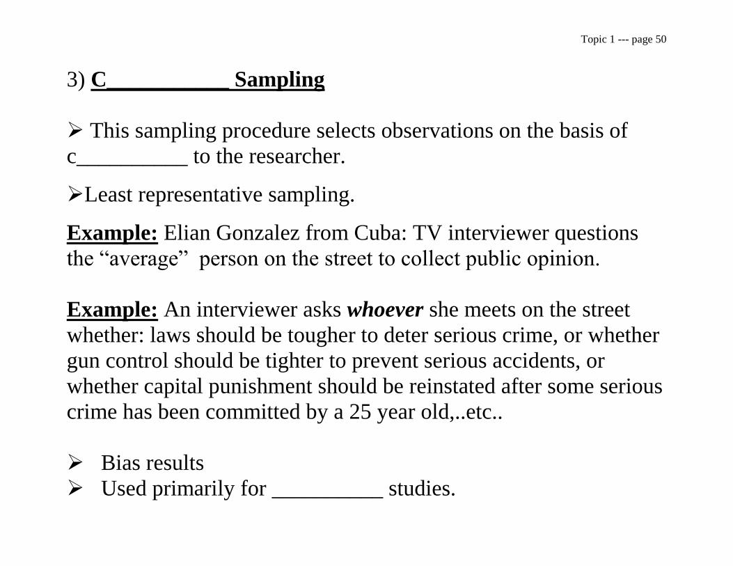
3) C___________ Sampling
This sampling procedure selects observations on the basis of
c__________ to the researcher.
Least representative sampling.
Example: Elian Gonzalez from Cuba: TV interviewer questions
the “average” person on the street to collect public opinion.
Example: An interviewer asks whoever she meets on the street
whether: laws should be tougher to deter serious crime, or whether
gun control should be tighter to prevent serious accidents, or
whether capital punishment should be reinstated after some serious
crime has been committed by a 25 year old,..etc..
Bias results
Used primarily for __________ studies.

Topic 1 --- page 51
Summary:
Statistical Sampling Procedures Probabilistic Non-Probabilistic
Topic 1 --- page 52
Sample Statistics
The primary objective of sampling from a population is to _____
something about that population.
The sample design determines the degree of ______ of on
gathered from the sample.
Next we will pull together sampling and the notion of probability
from Economics 245, to analyze sample results:
Topic 1 --- page 53
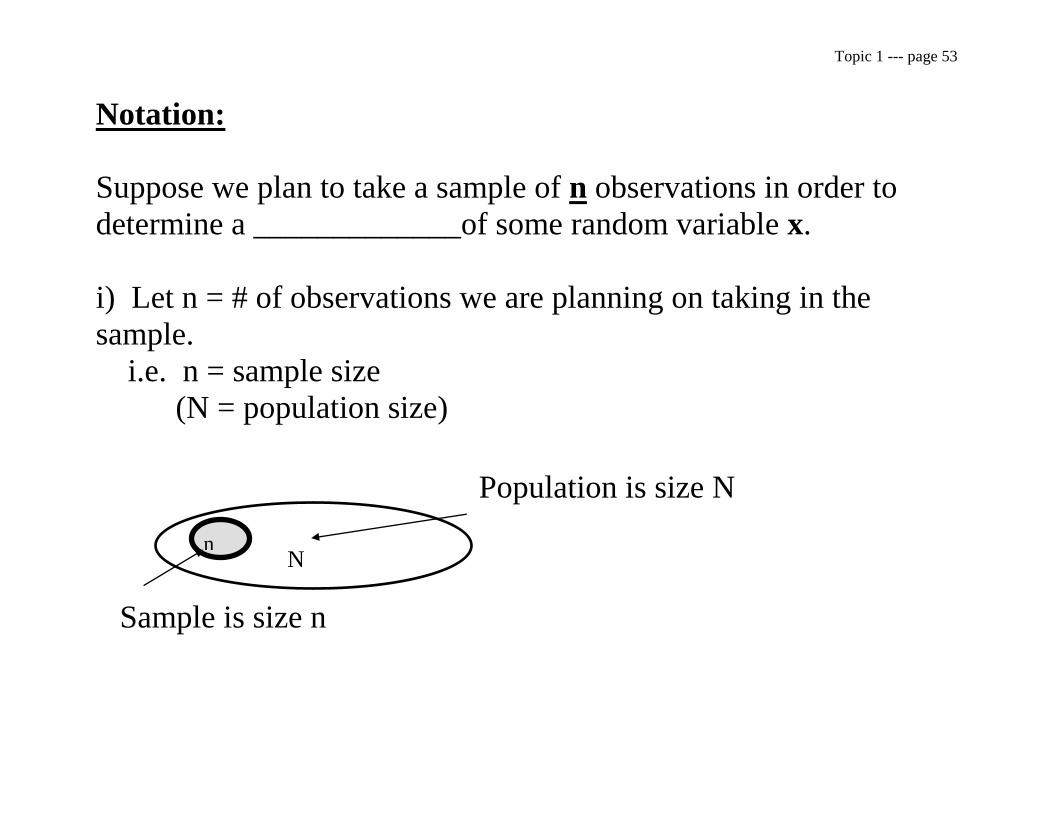
Notation:
Suppose we plan to take a sample of n observations in order to
determine a _____________of some random variable x.
i) Let n = # of observations we are planning on taking in the
sample.
i.e. n = sample size
(N = population size)
n N
Population is size N
Sample is size n
Topic 1 --- page 54
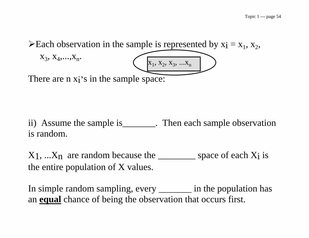
Each observation in the sample is represented by xi = x1, x2,
x3, x4,...,xn.
There are n xi’s in the sample space:
ii) Assume the sample is_______. Then each sample observation
is random.
X1, ...Xn are random because the ________ space of each Xi is
the entire population of X values.
In simple random sampling, every _______ in the population has
an equal chance of being the observation that occurs first.
x1, x2, x3, ...xn
Topic 1 --- page 55
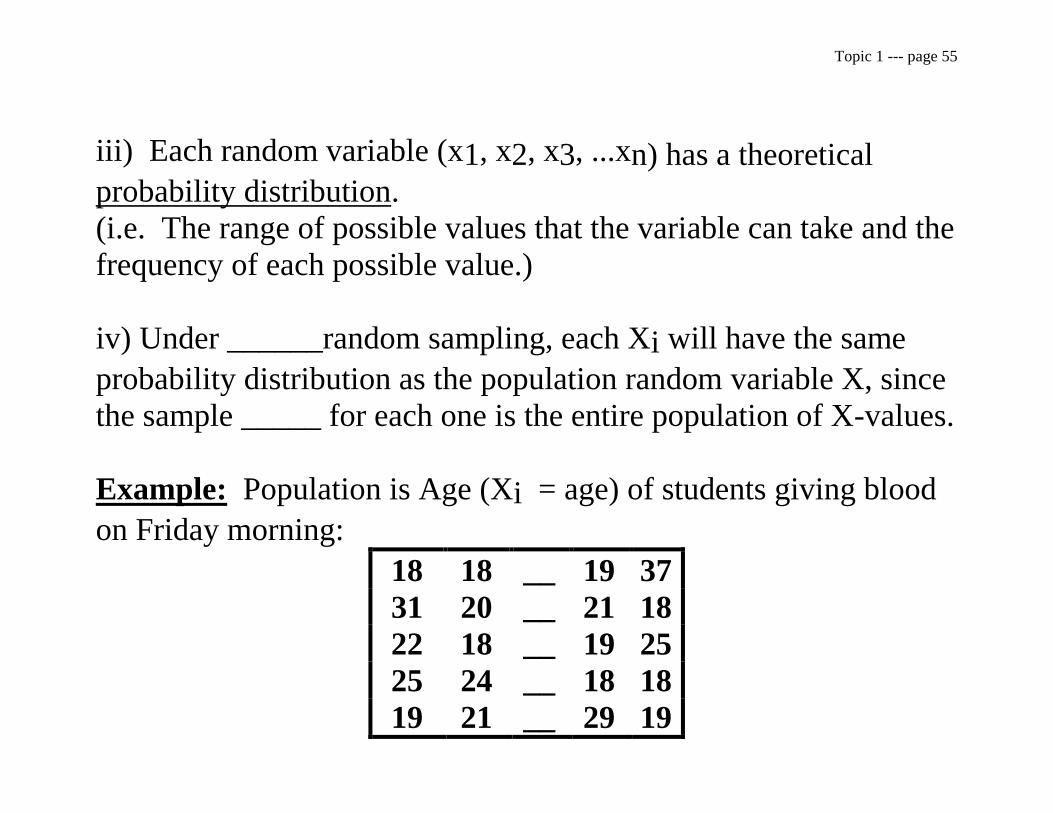
iii) Each random variable (x1, x2, x3, ...xn) has a theoretical
probability distribution.
(i.e. The range of possible values that the variable can take and the
frequency of each possible value.)
iv) Under ______random sampling, each Xi will have the same
probability distribution as the population random variable X, since
the sample _____ for each one is the entire population of X-values.
Example: Population is Age (Xi = age) of students giving blood
on Friday morning:
18 18 __ 19 37
31 20 __ 21 18
22 18 __ 19 25
25 24 __ 18 18
19 21 __ 29 19
Topic 1 --- page 56
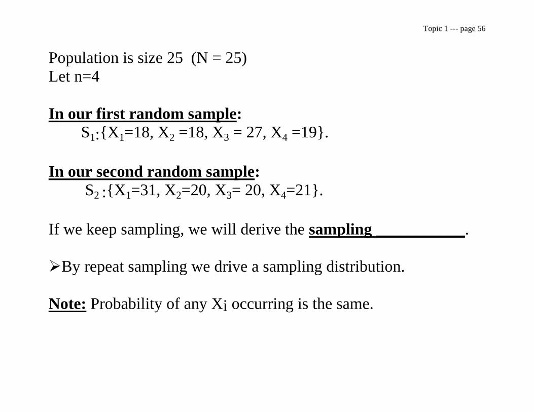
Population is size 25 (N = 25)
Let n=4
In our first random sample:
S1:{X1=18, X2 =18, X3 = 27, X4 =19}.
In our second random sample:
S2 :{X1=31, X2=20, X3= 20, X4=21}.
If we keep sampling, we will derive the sampling ___________.
By repeat sampling we drive a sampling distribution.
Note: Probability of any Xi occurring is the same.

Topic 1 --- page 57
Example:
__ __
__ __
N=4 and n=2
(Nn) pairs
All the possible samples of size n = 2 (with ___________) are:
{18, 21} {18, 25} {18, 19} {25, 18} {25, 19} {19, 21} {18, 18}
{21, 21}{21, 18} {21, 25} {21, 19} {25, 21} {19, 18} {19, 25}
{25, 25} {19, 19}
The average of each sample:
[19.5] [21.5] [18.5] [21.5] [22] [20] [18] [21]
[19.5] [23] [20] [23] [18.5] [22] [25] [19]
The population mean = ______;
The mean of all the samples taken together also = _____.

Topic 1 --- page 58
The population parameters of interest are usually a measure
of central location and dispersion.
Definitions:
(I) Population parameter is some characteristic of the population.
For example: = population mean;
2 = population variance;
= population proportion;
(II) A sample statistic is any ________ of the random sample
values.

Topic 1 --- page 59
Example from above:
18 21
25 19
Sample mean: X
nX
i
i
n
1
1
For a sample of size 2:
2
21XX
X
One possible random sample will have a sample mean equal to:
{(18+25)/2} = 21.5
Topic 1 --- page 60
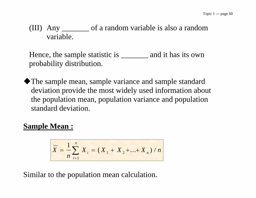
(III) Any _______ of a random variable is also a random
variable.
Hence, the sample statistic is _______ and it has its own
probability distribution.
The sample mean, sample variance and sample standard
deviation provide the most widely used information about
the population mean, population variance and population
standard deviation.
Sample Mean :
X
nX X X X n
i
i
n
n
1
1
1 2( ... ) /
Similar to the population mean calculation.
Topic 1 --- page 61
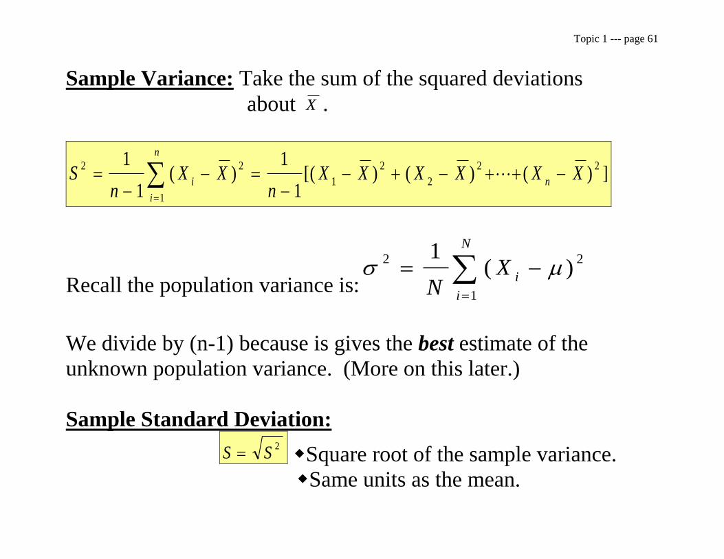
Sample Variance: Take the sum of the squared deviations
about X .
Sn
X Xn
X X X X X Xi
i
n
n
2 2
1
1
2
2
2 21
1
1
1
( ) [( ) ( ) ( ) ]
Recall the population variance is:
2 2
1
1
N
Xi
i
N
( )
We divide by (n-1) because is gives the best estimate of the
unknown population variance. (More on this later.)
Sample Standard Deviation:
S S2
Square root of the sample variance.
Same units as the mean.

Topic 1 --- page 62
Example: Price of ice cream 1 litre. We take a sample of 5
brands of ice cream to estimate the average cost of a
1 litre carton of ice cream.
Find the sample mean, variance and standard deviation:
Ice Cream i=brand Price (X)
in $
(Xi - X ) (Xi - X )
2
Compliments 1 [4.69-5.59]=-0.9 0.81 Island Farms 2 [3.99-5.59]=-1.6 2.56 Penny Lite 3 [4.29-5.59]=-1.3 1.69 Breyers’ 4 [5.99-5.59]=0.4 0.16 Dairy Queen 5 [8.99-5.59]=3.4 11.56
n=5 Xi =27.95 (Xi - X ) = 0 (Xi - X )2=16.78
X =5.59
Topic 1 --- page 63
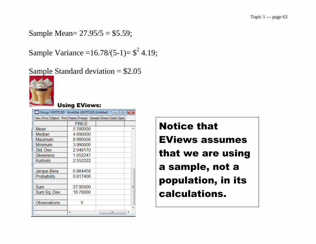
Sample Mean= 27.95/5 = $5.59;
Sample Variance =16.78/(5-1)= $2 4.19;
Sample Standard deviation = $2.05
Using EViews:
Notice that
EViews assumes
that we are using
a sample, not a
population, in its
calculations.
Topic 1 --- page 64
Sample Statistics Using Frequencies
Data are often presented in the form of a frequency
distribution.
That is, some values of Xi occur more than once.
The number of times Xi occurs (its frequency,) is denoted
as “ fi”.
If data is in the form of a frequency distribution, then we
make the following adjustments to our formulas:
Topic 1 --- page 65
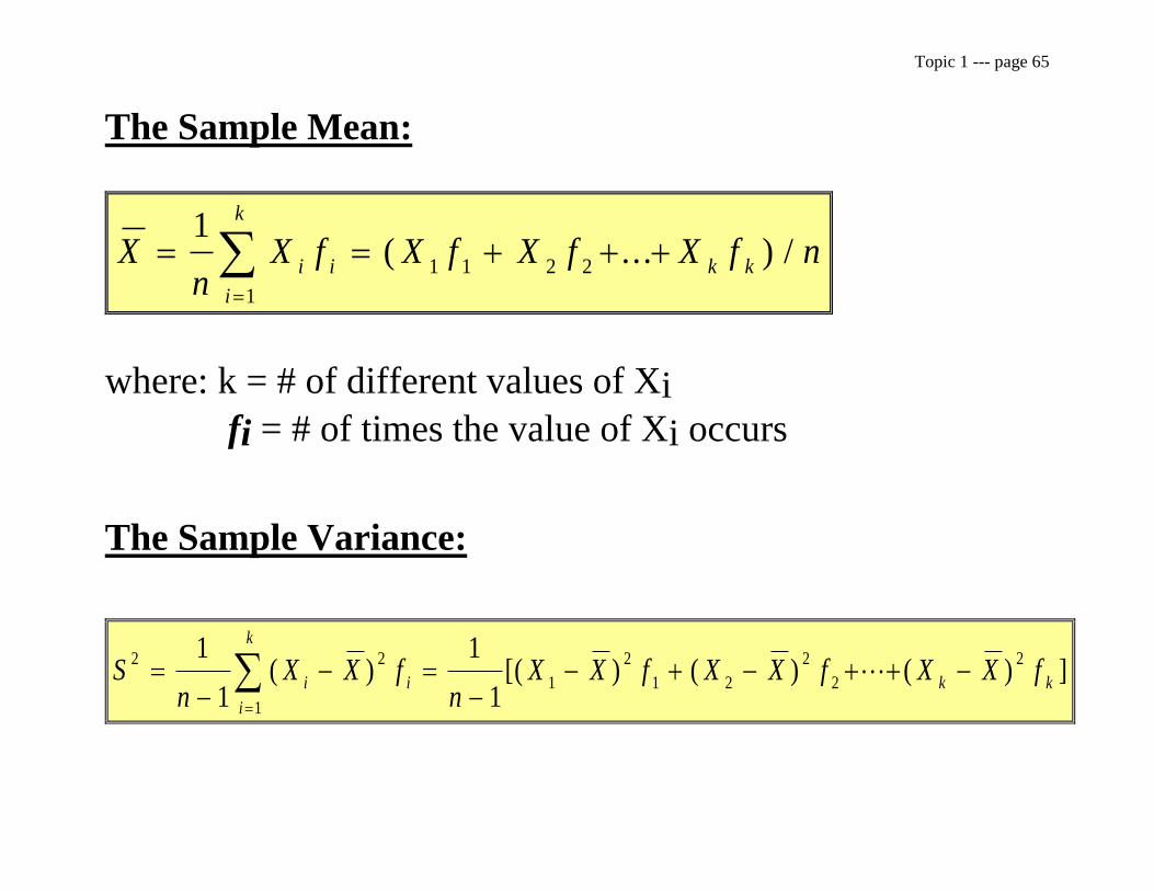
The Sample Mean:
Xn
X f X f X f X f ni i
i
k
k k
1
1
1 1 2 2( ... ) /
where: k = # of different values of Xi
fi = # of times the value of Xi occurs
The Sample Variance:
Sn
X X fn
X X f X X f X X fi i
i
k
k k
2 2
1
1
2
1 2
2
2
21
1
1
1
( ) [( ) ( ) ( ) ]
Topic 1 --- page 66
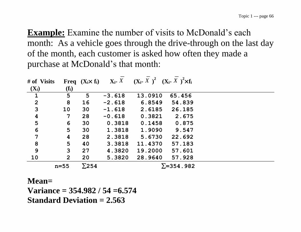
Example: Examine the number of visits to McDonald’s each
month: As a vehicle goes through the drive-through on the last day
of the month, each customer is asked how often they made a
purchase at McDonald’s that month:
# of Visits Freq (Xi× fi) Xi- X (Xi- X )2 (Xi- X )
2×fi
(Xi) (fi)
1 5 5 -3.618 13.0910 65.456
2 8 16 -2.618 6.8549 54.839
3 10 30 -1.618 2.6185 26.185
4 7 28 -0.618 0.3821 2.675
5 6 30 0.3818 0.1458 0.875
6 5 30 1.3818 1.9090 9.547
7 4 28 2.3818 5.6730 22.692
8 5 40 3.3818 11.4370 57.183
9 3 27 4.3820 19.2000 57.601
10 2 20 5.3820 28.9640 57.928
n=55 254 =354.982
Mean=
Variance = 354.982 / 54 =6.574
Standard Deviation = 2.563

Topic 1 --- page 67
Concluding Note:
Recall, the objective in calculating sample statistics (mean,
variance, standard deviation), is to ________ population
parameters.
When we take samples from a population, we may end up
with ______ results each time we take a different sample.
The only way to determine the true population parameters
is to take account of every _______ in the population
(census).
Problem: Census is too expensive.

Topic 1 --- page 68
Thus, we must accept that _______ statistics generated
from sampling will be used to estimate population
parameters, and we must make statements on how _______or
accurate such sample statistics are in describing population
parameters.

Topic 1 --- page 69
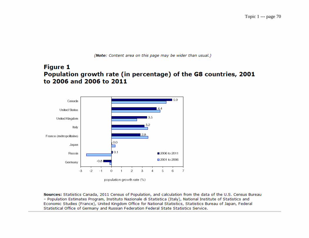
Topic 1 --- page 70

Topic 1 --- page 71
Topic 1 --- page 72
Probability Distribution of A Statistic
Sampling Distribution of X
Each sample statistic is a random variable.
Recall from the notes:
i) Let n = # of observations we are planning on taking in the
sample.
i.e. n = sample size
(N = population size)
Each observation in the sample is represented by xi = x1, x2,
...,xn.
There are n xi’s in the sample space.
Topic 1 --- page 73
ii) Assume the sample is _______. Then each sample observation
is random.
X1, ...Xn are _______because the sample space of each Xi is
the entire population of X values.
In simple ________sampling, every element in the population
has an equal chance of being the observation that occurs first.
iii) Each random variable (x1, x2, x3, ...xn) has a theoretical
probability distribution. (i.e. The range of possible values that the
variable can take and the frequency of each possible value.)
iv) Under simple random sampling, each Xi will have the same
probability distribution as the population random variable X, since
the sample space for each one is the entire population of X-values.
Therefore, each _______ has its own probability distribution.

Topic 1 --- page 74
The probability distribution of a sample statistic is called its:
“sampling distribution.”
So it is legitimate to ask:
“What is the expected value of X [E( X )]?
Or
“What is the variance of X [V( X )]?
The results help determine how “reliable” or ______ our sample
statistics are as measures of the corresponding population
parameters.
i.e. How good are our estimates of the population parameters.
Topic 1 --- page 75
Recall:
(i) Each sample we draw from a particular population will have its
own _______ statistic.
i.e. For a particular sample, it will have a particular derived
sample mean, sample variance, etc..
(ii) Usually each sample implies a different statistical value.
i.e. Each sample will have a different sample mean, sample
variance, etc..
Topic 1 --- page 76
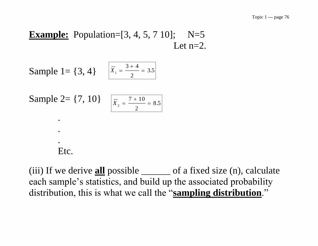
Example: Population=[3, 4, 5, 7 10]; N=5
Let n=2.
Sample 1= {3, 4} X1
3 4
23 5
.
Sample 2= {7, 10} X
2
7 10
28 5
.
.
.
.
Etc.
(iii) If we derive all possible ______ of a fixed size (n), calculate
each sample’s statistics, and build up the associated probability
distribution, this is what we call the “sampling distribution.”
Topic 1 --- page 77
Illustration: Sampling Distribution of X (the Sample Mean)
“The sampling distribution of X is the probability distribution of
all possible values of X that could occur when a ______ of size n
is taken from some specified population.”
Note: A sampling distribution is a __________because it contains
all the possible values of some sample statistic.
(Population of X ={ X1 , X
2 , X3 ,… X
k })
Topic 1 --- page 78
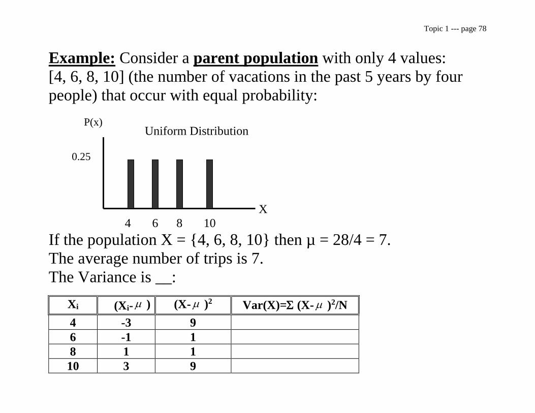
Example: Consider a parent population with only 4 values:
[4, 6, 8, 10] (the number of vacations in the past 5 years by four
people) that occur with equal probability:
X
4 6 8 10
If the population X = {4, 6, 8, 10} then µ = 28/4 = 7.
The average number of trips is 7.
The Variance is __:
Xi (Xi- ) (X- )2 Var(X)= (X- )2/N
4 -3 9
6 -1 1
8 1 1
10 3 9
P(x)
0.25
Uniform Distribution
Topic 1 --- page 79
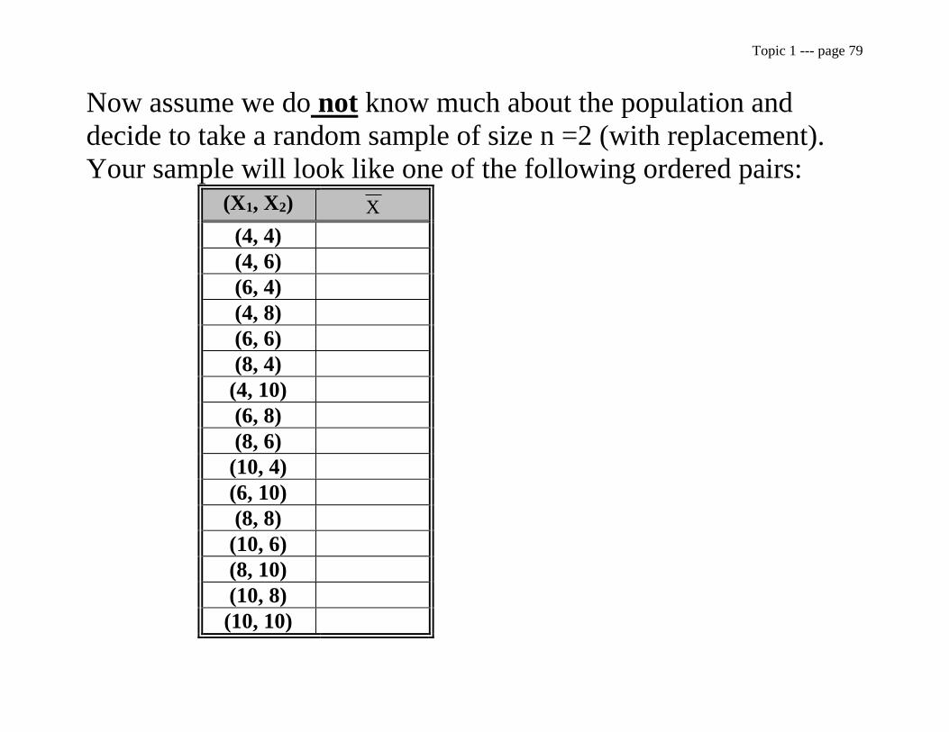
Now assume we do not know much about the population and
decide to take a random sample of size n =2 (with replacement).
Your sample will look like one of the following ordered pairs: (X1, X2) X
(4, 4)
(4, 6)
(6, 4)
(4, 8)
(6, 6)
(8, 4)
(4, 10)
(6, 8)
(8, 6)
(10, 4)
(6, 10)
(8, 8)
(10, 6)
(8, 10)
(10, 8)
(10, 10)

Topic 1 --- page 80
Sampling Distribution of X for n= 2 when X ={4, 6, 8,10}:
X P( X )
116
216
18
316
416
14
316
216
18
116
316
Probability
Distribution of X
for n=2
216
116
4 5 6 7 8 9 10 X
164

Topic 1 --- page 81
Mean of The Sample Mean X
Notation: Let X denote the “mean of the sampling
distribution of X .”
I.e. It is the mean of all possible sample means (the population of
X -values).
So :
E X X P X
X i i
i
k
( ) ( )
1
where i=1, 2, ….k, and k is the number of distinct possible
values of X .

Topic 1 --- page 82
In our last example k=7 :
E X( ) ( ) ( ) ( ) ( )
( ) ( ) ( )
4 116
5 216
6 316
7 416
8 316
9 216
10 116
7
So for the population:
X 7
It is not a coincidence that these 2 _____ are equal!!
X
for any parent population and any given sample
size.

Topic 1 --- page 83
Hence, if µ is the mean of the population of X’s and X
is the mean of the population of X ’s, then the expected value
of X :
E X
X( )
Proof:
Let Xi ~( X , 2
) for all i X is an independently
distributed random
variable, with a mean
of X and variance of
2.
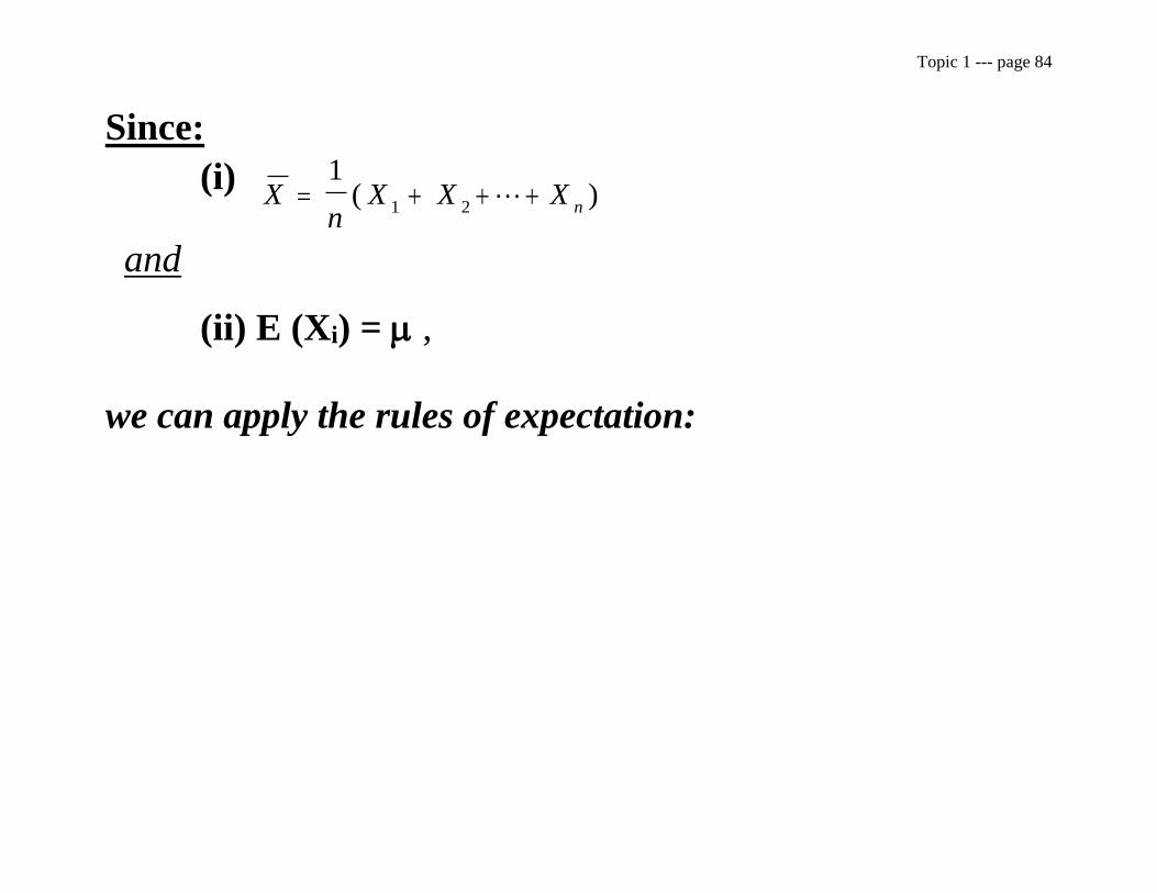
Topic 1 --- page 84
Since:
(i) X
nX X X
n
11 2
( )
and
(ii) E (Xi) = ,
we can apply the rules of expectation:

Topic 1 --- page 85
E X En
X
nE X
nE X X X
nE X E X E X E X
n
nn
i
i
n
i
i
n
n
n
X
( )
. #
1
1
1
1
1
1
1
1
1 2
1 2 3
Take the expectation operator
through and pull n out.
Expand
Take the expectation
operator through.
Replace
with
n’s cancel
Topic 1 --- page 86
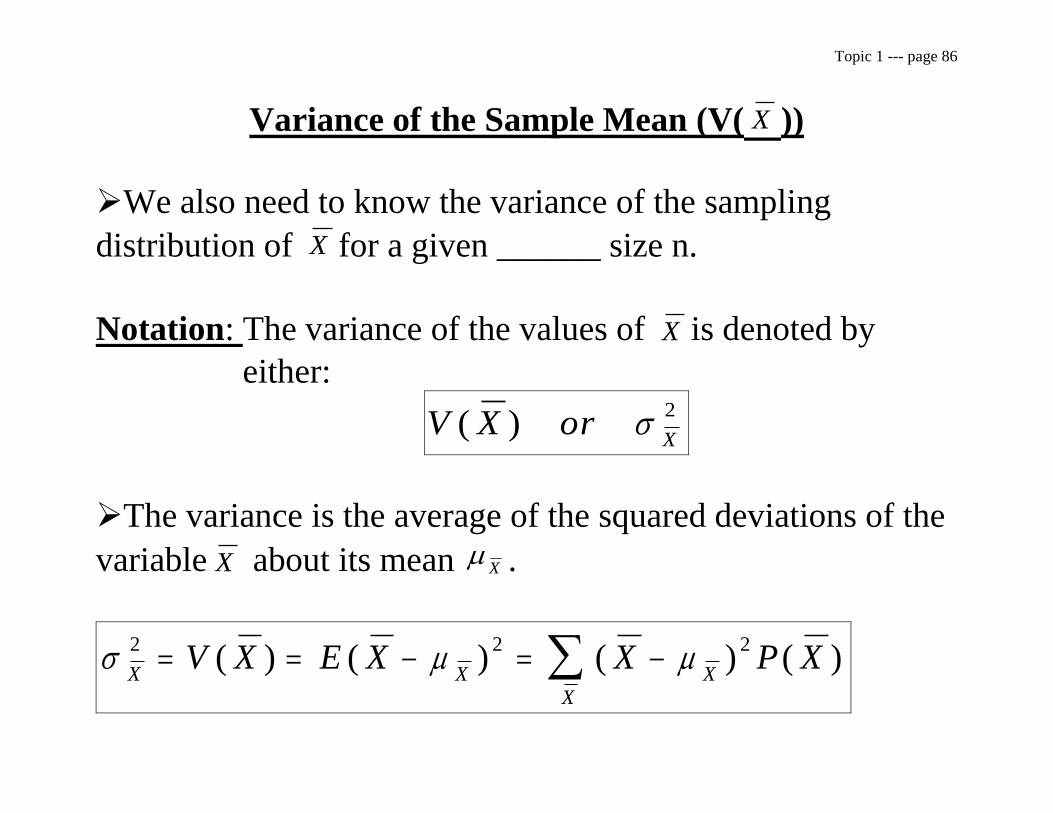
Variance of the Sample Mean (V( X ))
We also need to know the variance of the sampling
distribution of X for a given ______ size n.
Notation: The variance of the values of X is denoted by
either:
V X orX
( ) 2
The variance is the average of the squared deviations of the
variable X about its mean X .
X X X
X
V X E X X P X2 2 2 ( ) ( ) ( ) ( )
Topic 1 --- page 87
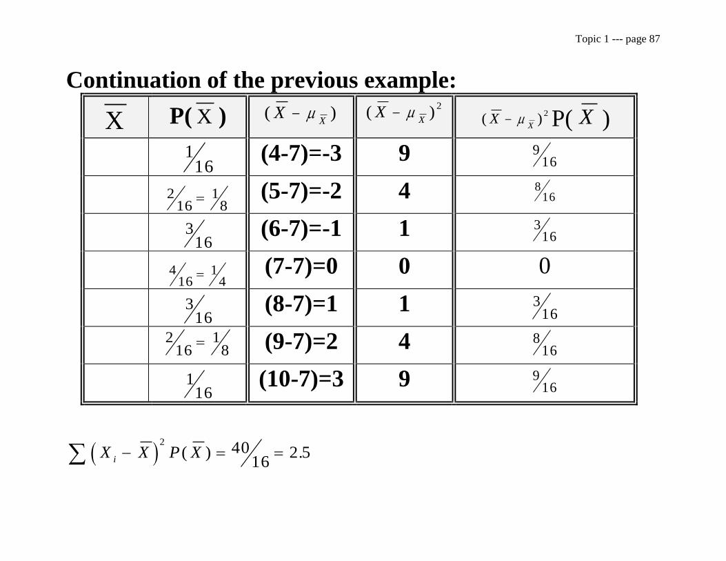
Continuation of the previous example:
X P( X ) ( )XX
( )XX
2
( )XX
2 P( X )
116
(4-7)=-3 9 916
216
18
(5-7)=-2 4 816
316
(6-7)=-1 1 316
416
14
(7-7)=0 0 0
316
(8-7)=1 1 316
216
18
(9-7)=2 4 816
116
(10-7)=3 9 916
X X P Xi
240
162 5( ) .
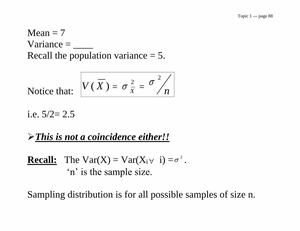
Topic 1 --- page 88
Mean = 7
Variance = ____
Recall the population variance = 5.
Notice that: V X
nX( ) 2
2
i.e. 5/2= 2.5
This is not a coincidence either!!
Recall: The Var(X) = Var(Xi i) =2.
‘n’ is the sample size.
Sampling distribution is for all possible samples of size n.

Topic 1 --- page 89
Proof:
V X Vn
X
nV X
nV X
and Since X s are independent under random sampling
n
nn
n
i
i
i
i
( )
( )
' :
.
1
1
1
1
1
1
2
2
2
2 2 2 2
2
2
2
Topic 1 --- page 90
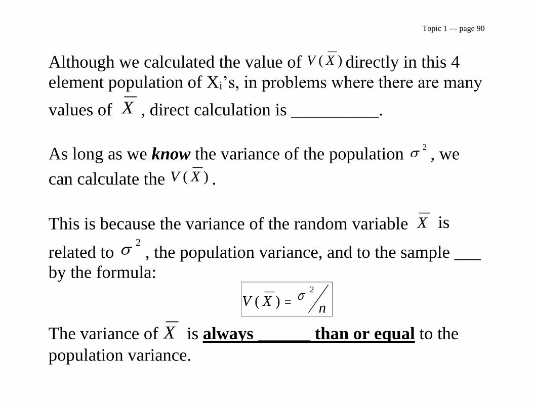
Although we calculated the value of V X( ) directly in this 4
element population of Xi’s, in problems where there are many
values of X , direct calculation is __________.
As long as we know the variance of the population 2
, we
can calculate the V X( ) .
This is because the variance of the random variable X is
related to 2
, the population variance, and to the sample ___
by the formula:
V Xn
( ) 2
The variance of X is always ______ than or equal to the
population variance.
Topic 1 --- page 91
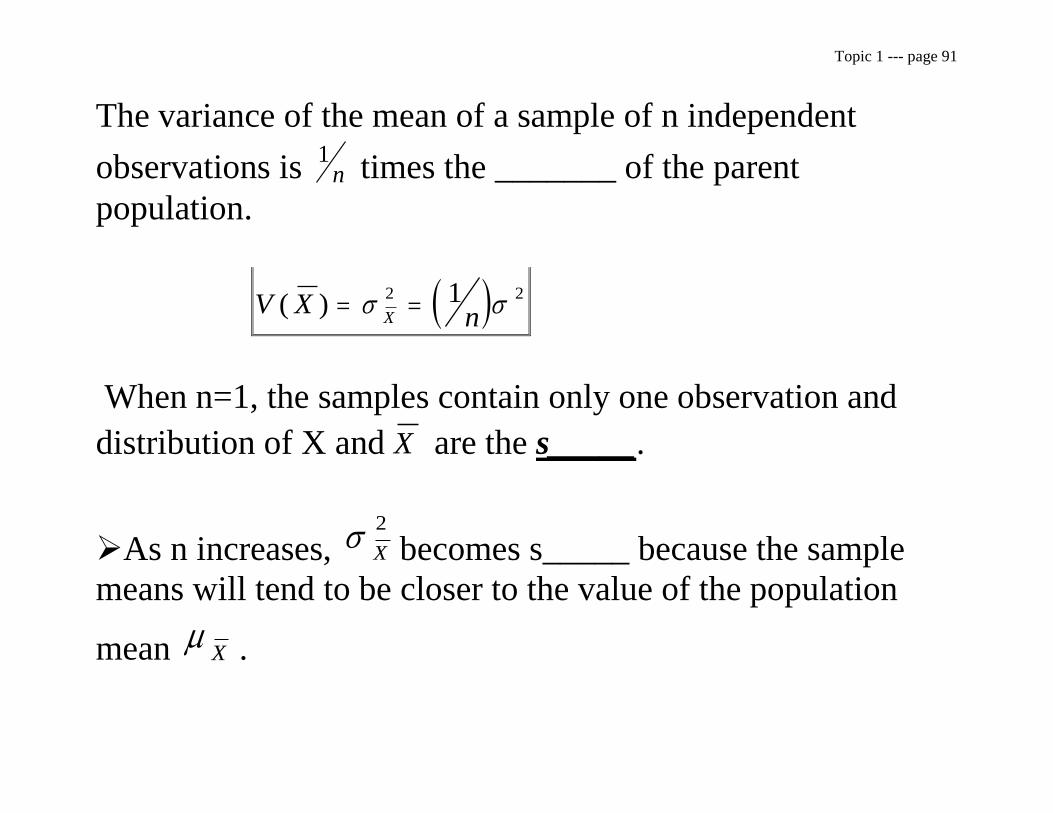
The variance of the mean of a sample of n independent
observations is 1
n times the _______ of the parent
population.
V XnX
( ) 2 21
When n=1, the samples contain only one observation and
distribution of X and X are the s_____.
As n increases, X
2
becomes s_____ because the sample
means will tend to be closer to the value of the population
mean X .

Topic 1 --- page 92
When n = N (in a finite population) all sample means will
equal the population mean and the V X( ) ’s will equal 0.
With our example, the population variance (2
) is known
(= 5) and n=2:
So the variance of X (V X( ) ) is:
V XnX
( ) . 2 21 1
25 2 5

Topic 1 --- page 93
What Happens toV X( ) as n Increases?
Because each sample contains more information or more
elements of the population as the sample size increases, the
sample will be closer to the population, so expect less
_________.
Example: Suppose X ~N(0, 100)
Randomly draw samples of size:
(i) 10
(ii) 100
(iii) 1000
from this population.
Topic 1 --- page 94
Calculate X 10 for all possible samples of size 10.
Calculate X 100 for all possible samples of size 100.
Calculate X 1000 for all possible samples of size 1000.
Then we can show:
For n=10: dispersion if X is quite wide around the mean of
0.
For n=1000: less variation around the mean of zero.
When n approaches infinity, there is no dispersion and
variance of X =0.
Topic 1 --- page 95
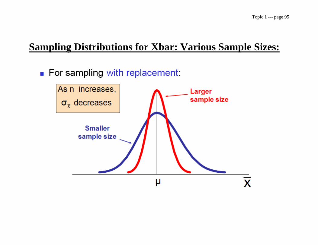
Sampling Distributions for Xbar: Various Sample Sizes:

Topic 1 --- page 96
Topic 1 --- page 97
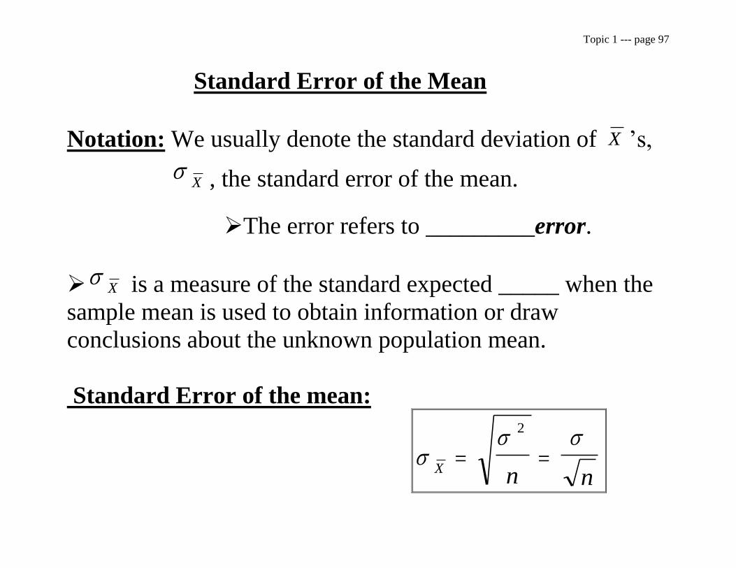
Standard Error of the Mean
Notation: We usually denote the standard deviation of X ’s,
X , the standard error of the mean. The error refers to _________error.
X is a measure of the standard expected _____ when the
sample mean is used to obtain information or draw
conclusions about the unknown population mean.
Standard Error of the mean:
X n n
2

Topic 1 --- page 98
In our example:
X n
25
2
2 236
215811
..
Notes: (i) X and X are parameters of the population of
sample averages for all conceivable samples of
size n.
These parameters are usually ________.
(ii) The population parameters (μ, σ2) are also usually
________.
(iii) This means that we cannot use the relationships:
X X
andn to solve for values of one of
these statistics.
Topic 1 --- page 99
But these relationships allow us to test hypotheses about the
population parameters on the basis of _______ results.
More on this later........
Next: We now have derived the mean and the variance of the
sampling distribution, but have not said anything about the
s____ of the sampling distribution of X .
Recall that distributions with the same mean and variance can
have very different ________.
We must now specify an assumption about the entire
distribution of X ’s:
Topic 1 --- page 100
Sampling distribution of X , Normal Parent Population
It is typically not possible to specify the shape of the
X ’s when the parent population is _______ and the sample
____ is small.
However, the shape of a sample taken from a normally
distributed parent population (X) can be specified.
In this case, the X ’s are distributed _________.
“ The sampling distribution of X ’s drawn from a normal
parent population is a normal distribution.”
Recall: The mean of the X s is X and the variance of
X s is X n2
2
.
Topic 1 --- page 101
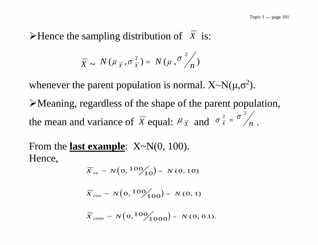
Hence the sampling distribution of X is:
X ~ N NnX X
( , ) ( , ) 22
whenever the parent population is normal. X~N(μ,σ2).
Meaning, regardless of the shape of the parent population,
the mean and variance of X equal: X and
X n2
2
.
From the last example: X~N(0, 100).
Hence,
X N N
X N N
X N N
10
100
1000
0 10010
0 10
0 100100
0 1
0 1001000
0 0 1
~ , ( , )
~ , ( , )
~ , ( , . ).

Topic 1 --- page 102
Remember: The normal distribution is a continuous
distribution. (I.e. infinite number of different samples could
be drawn.)
Example: Suppose all the possible samples of size 10 are
drawn from a normal distribution that has a mean of 25 and a
variance of 50. That is, X is normally distributed with a mean
μ=25 and variance σ2=50 : X~N(25,50).
Since the population mean μ=25, the ____of X s equal
X =25.
Since the population variance σ2=50, the _______ of the
X ’s equals
X n2
250
105 .
Since X is normal, X is normally distributed X ~N(25,5).

Topic 1 --- page 103
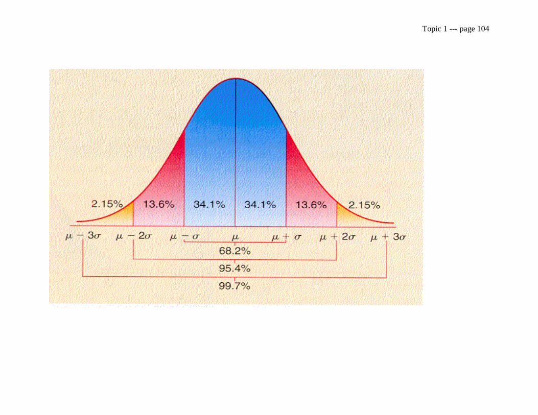
What this means is:
68.3% of the sample means will fall within ± one standard
error of the mean: X 5 2 24. .
1 25 1 2 24 22 76 27 24X
to( )( . ) . . .
95.43% of the sample means will fall within ± two standard
errors of the mean:
2 25 2 2 24 25 4 48 20 52 29 48X
to( )( . ) . . . .
99.7% of the sample means will fall within ± three standard
errors of the mean:
3 25 3 2 24 25 6 72 18 28 3172X
to( )( . ) . . . .
Topic 1 --- page 104
Topic 1 --- page 105
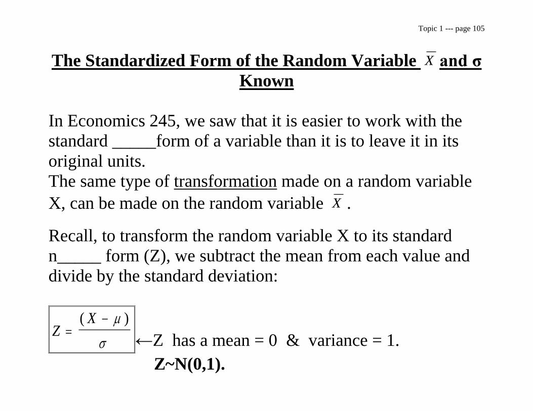
The Standardized Form of the Random Variable X and σ
Known
In Economics 245, we saw that it is easier to work with the
standard _____form of a variable than it is to leave it in its
original units.
The same type of transformation made on a random variable
X, can be made on the random variable X .
Recall, to transform the random variable X to its standard
n_____ form (Z), we subtract the mean from each value and
divide by the standard deviation:
ZX
( )
←Z has a mean = 0 & variance = 1.
Z~N(0,1).
Topic 1 --- page 106
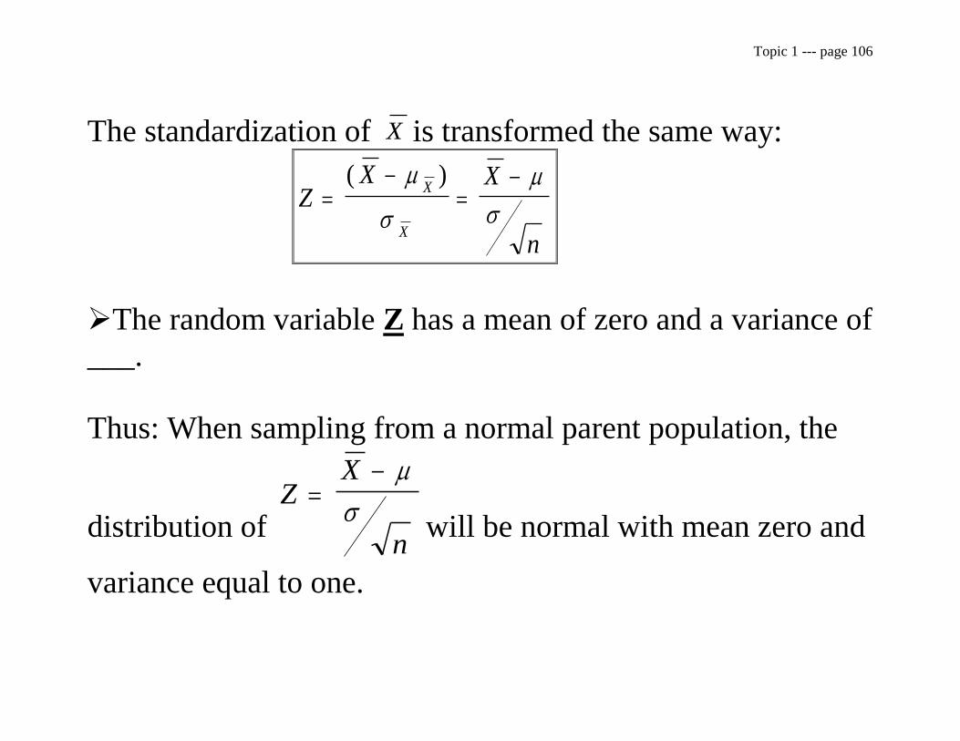
The standardization of X is transformed the same way:
Z
X X
n
X
X
( )
The random variable Z has a mean of zero and a variance of
___.
Thus: When sampling from a normal parent population, the
distribution of Z
X
n
will be normal with mean zero and
variance equal to one.

Topic 1 --- page 107

Topic 1 --- page 108
Example: Suppose X is the height (in inches) of basketball
players on all university teams in Canada during summer
term.
Suppose X~N(75,36). A random sample of nine players is
drawn from this population.
What is the probability that the sample average team
player height is less than 80 inches? (What is P ( X ≤ 80)?)
Solution: If X ~N(75,36), then X ~N(75,36/9=4).
Standardize the variable X :
Z
X
n
80 75
69
5
63
5
22 5.

Topic 1 --- page 109
Looking at the Cumulative Standardized Normal Distribution
Table F(Z), the P(Z ≤2.5) =______.
The probability that the average height of basketball players
in our sample of size 9 is less than 80 inches is ____%.
Z 0 2.5
0.9938=CDF
Topic 1 --- page 110
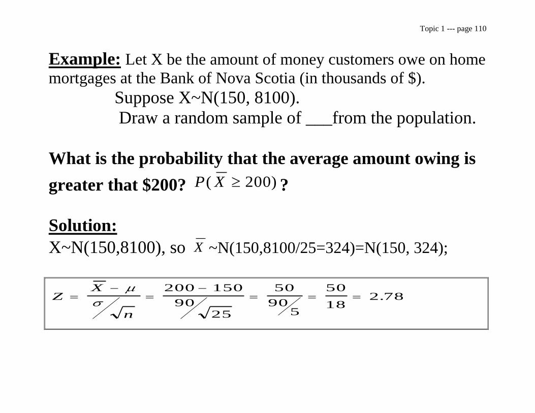
Example: Let X be the amount of money customers owe on home
mortgages at the Bank of Nova Scotia (in thousands of $).
Suppose X~N(150, 8100).
Draw a random sample of ___from the population.
What is the probability that the average amount owing is
greater that $200? P X( ) 200 ?
Solution:
X~N(150,8100), so X ~N(150,8100/25=324)=N(150, 324);
ZX
n
200 150
9025
50
905
50
182 78.

Topic 1 --- page 111
P(Z ≥2.78) = (1-0.9973) = 0.0027.
The probability that average amount owing on a
mortgage is greater that $200 is .27%.
Z
2.78
0.9973=CDF
0.0027

Topic 1 --- page 112
The limitations from the last section is obvious:
“ We cannot always assume that the parent population is
_______.”
What if the Population is Non-Normal?

Topic 1 --- page 113
Sampling Distribution of X : Population Distribution
Unknown and σ Known
When the samples drawn are not from a normal population
or when the population distribution is unknown, the ____ of
the sample is extremely important.
When the sample ____is small, the shape of the
distribution will depend mostly on the shape of the parent
population.
As the sample ____ increases, the shape of the sampling
distribution of X will become more and more like a normal
distribution, regardless of the shape of the parent population.

Topic 1 --- page 114
Central Limit Theorem:
“Regardless of the distribution of the parent
population, as long as it has a finite mean µ and
variance σ2, the distribution of the means of the
random samples will approach a normal distribution,
with mean μ and variance σ2/n, as the sample size n,
goes to infinity.”
(I) When the parent population is ______, the sampling
distribution of X is exactly normal.
(II) When the parent population is not _______or unknown,
the sampling distribution of X is approximately normal as
the sample size increases.
Topic 1 --- page 115
Example:
Let the sample be (X1, X2, ... ,Xn)
Let S=(X1 + X2 + X3+...+Xn)
E(S) = E(X1) + E(X2) + ... +E(Xn)
=ΣE(Xi) = n(E(X)=nμ
V(S) = V(X1 + X2 + ...+ Xn) = V(X1) +V(X2) + ...+V( Xn)
=ΣV(Xi) = nV(Xi) = nσ2.
Assuming independence.
So according to the CLT as n →
S → N(nμ, nσ2)

Topic 1 --- page 116
Now, X
nX
X X X
n
S
ni
i
n
n
1
1
1 2( )
.
The expected value of X is:
E Xn
E Sn
n
and the iance of X
V X VS
n nV S
nn
n
( ) ( )
var :
( ) ( ) .
1 1
1 12 2
2
2
So, according to the CLT: as n → , X ~N(μ, σ2/n)
regardless of the form of the parent population distribution.

Topic 1 --- page 117
(Note: the CLT applies in discrete and continuous cases.)

Topic 1 --- page 118
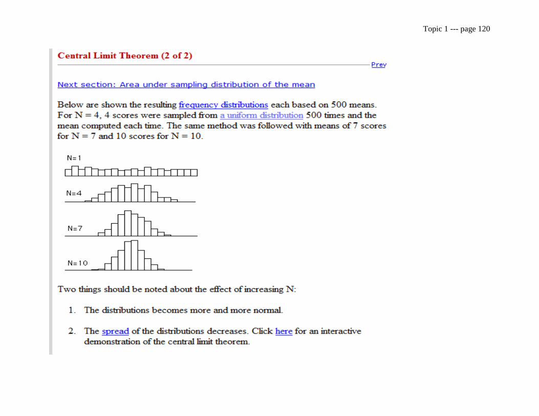
The first row of diagrams shows different parent
populations.
The next 3 rows show the sampling distribution of
X for all possible repeated samples of size n=2, n=5, and
n=30, drawn from the populations in the first row.
Column 1 : Uniform Population
At n=2, symmetrical
At n=5, normal looking distribution
Column 2: Bimodal Population
At n=2 the distribution is symmetrical.
At n=5, the distribution is bell-shaped.

Topic 1 --- page 119
Column 3 Highly skewed exponential Population.
At n=2 and n=5, the distribution is still skewed.
At n=30, symmetrical bell-shaped distribution for
X → normal.
In General, if n ≥ 30, the sampling distribution of X will be a
good approximation.
Topic 1 --- page 120

Topic 1 --- page 121

Topic 1 --- page 122
Topic 1 --- page 123
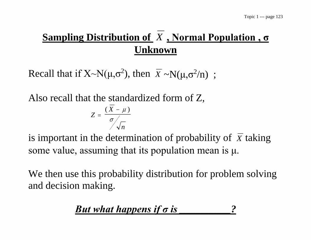
Sampling Distribution of X , Normal Population , σ
Unknown
Recall that if X~N(μ,σ2), then X ~N(μ,σ2/n) ;
Also recall that the standardized form of Z,
Z
X
n
( )
is important in the determination of probability of X taking
some value, assuming that its population mean is μ.
We then use this probability distribution for problem solving
and decision making.
But what happens if σ is __________?

Topic 1 --- page 124
In solving a problem where σ is u_______, ‘s’, the sample
statistic for standard deviation of σ, can be applied to solve
problems involving standardization.
It is legitimate because it can be shown that: E(S2)=σ2
and we can standardize creating a new ratio:
t
X
sn
.
Where “t-ratio” is not _________ distributed.
The resulting distribution no longer has a _______equal to
1.

Topic 1 --- page 125
To determine the distribution of the ratio X
sn
we follow
these steps:
1) Collect all the possible samples of size n from a normal
parent population.
2) Calculate X and s for each sample.
3) Subtract μ from each value of X , and then divide this
deviation by the appropriate value of s
n.
This process will generate an infinite number of values of this
random variable
X
sn
.
Topic 1 --- page 126
The mean of the t-distribution still equals 0.
The variance no longer equals V(Z) = 1. It is larger.
Because we use ‘s’ to standardize, the dispersion or the
variation around the mean zero, will be wider.
“s” introduces an element of uncertainty or _____because
s2 is a parameter estimate, not the actual population
parameter.
Hence the more uncertainty there is, the more spread out the
distribution.
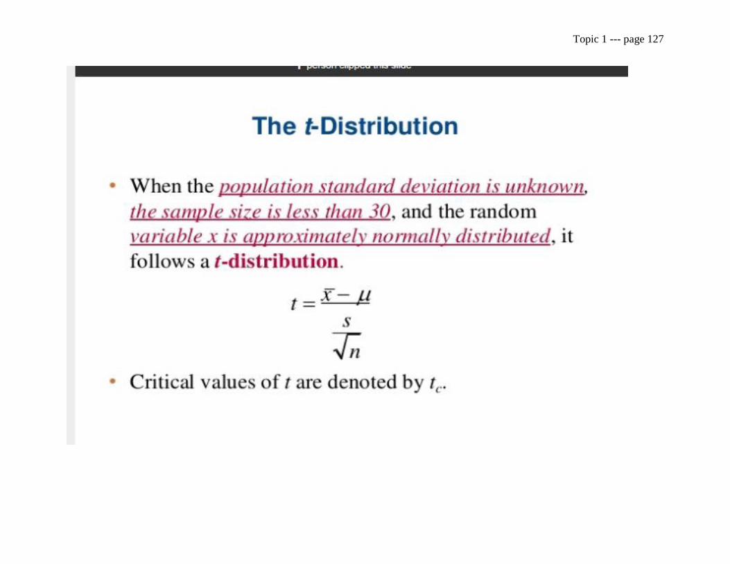
Topic 1 --- page 127

Topic 1 --- page 128

Topic 1 --- page 129
Topic 1 --- page 130
Notes About The t- Distribution:
1) The t-distribution was developed by W.S. Gossett.
It consists of two random variables X and s. Hence, the
variable “t” is a continuous random variable.
2) [ ] t Cumulative probability.
3) The t-distribution is _________: E(t) =0= median = mode.
4) Variability of the t-distribution depends on the sample size
(n), since n affects the reliability of the estimate of ‘σ’
which ‘s’ estimates.
When n is large, ‘s’ will be a good estimator of σ.
When n is small, ‘s’ may not be a good estimator.
Topic 1 --- page 131
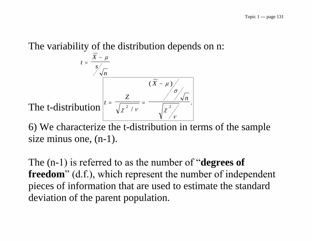
The variability of the distribution depends on n:
tX
sn
The t-distribution t
Z
X
n
2 2/
( )
.
6) We characterize the t-distribution in terms of the sample
size minus one, (n-1).
The (n-1) is referred to as the number of “degrees of
freedom” (d.f.), which represent the number of independent
pieces of information that are used to estimate the standard
deviation of the parent population.

Topic 1 --- page 132
ν ← “nu” denotes degrees of freedom: ν=(n-1).
t-distribution is described by ν ___________of______.
(i) The mean of t-distribution =0; [E(t) = 0].
(ii) The variance for n≥3, is V tn
n
n
n( )
( )
( )
( )
( )
( ).
2
1
1 2
1
3
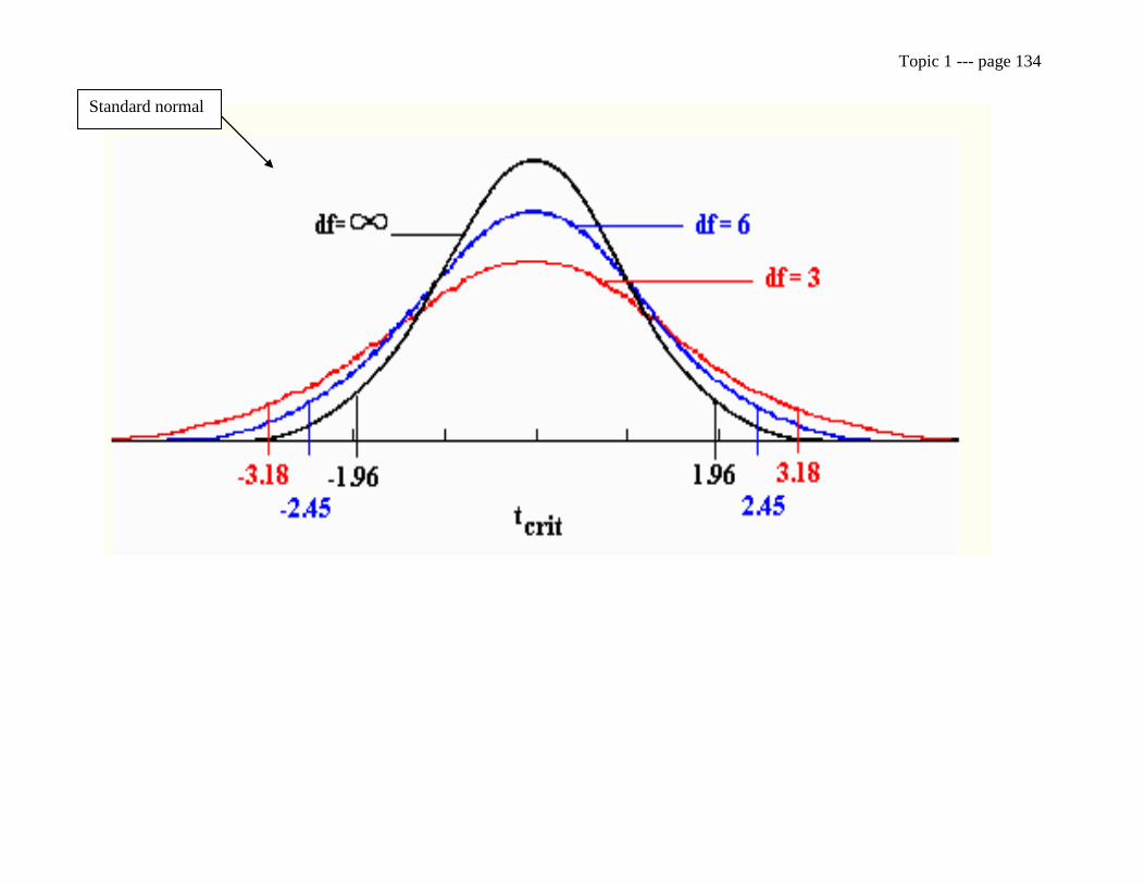
7) For small sample ____, the t-distribution is typically more
spread out than the normal distribution.
t-distribution typically has fatter tails than the Z for small
degrees of freedom.
When the degrees of freedom are larger than ___, the t
distribution resembles the normal distribution.

Topic 1 --- page 133
In the limit, as n approaches infinity, the t and Z
distributions are the same.
So, the t-tables usually have probability values for 30 ,
since larger samples normally give a good approximation and
are easier to use.
Although the distribution holds for any sample size, we
usually use the t-distribution when we are using small
samples.
Topic 1 --- page 134
Standard normal

Topic 1 --- page 135
Probability Applications:
Probability questions involving a t-distributed random
variable can be solved by forming the t-statistic: t
X
sn
,
and determining the probability by using the Student t-table
or a computer generated value (using the @ctdist(x,ν)
command in EViews).
The Student t-table gives the values of “t” for selected
values of the probability 1-F(t)=1-P(t<t)=P(t>tv, )= across
the top of the table and for degree of freedom (ν) down the
left margin.

Topic 1 --- page 136
Table gives probabilities for selected t-values for each
degree of freedom.
More extensive tables are available.
The easiest way to determine probabilities is to use a
statistical package.
0 1.318 tν=24
Recall, the t-distribution is the appropriate statistic for
inference on a population mean whenever the parent
population is normally distributed and σ is unknown.
F(1.318)=0.90 α=1-F(tν)
Topic 1 --- page 137
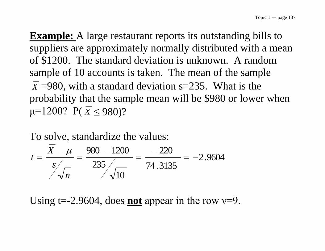
Example: A large restaurant reports its outstanding bills to
suppliers are approximately normally distributed with a mean
of $1200. The standard deviation is unknown. A random
sample of 10 accounts is taken. The mean of the sample
X =980, with a standard deviation s=235. What is the
probability that the sample mean will be $980 or lower when
μ=1200? P( X ≤ 980)?
To solve, standardize the values:
9604.23135.74
220
10235
1200980
ns
Xt
Using t=-2.9604, does not appear in the row ν=9.

Topic 1 --- page 138
Use table to determine an upper and lower bound for
P(t<-2.9604):
F(-2.821) = 0.01
F(-3.250) = 0.005
0.005 ≤ P(t≤-2.9604) ≤ 0.01.
A sample mean as low or lower than 980 will occur
approximately between 1% to 0.5% of the time with
μ=$1200.
May be concerned with the accuracy of the sample.

Topic 1 --- page 139
Using EViews :
According EViews, the probability is 0.798%.
Topic 1 --- page 140
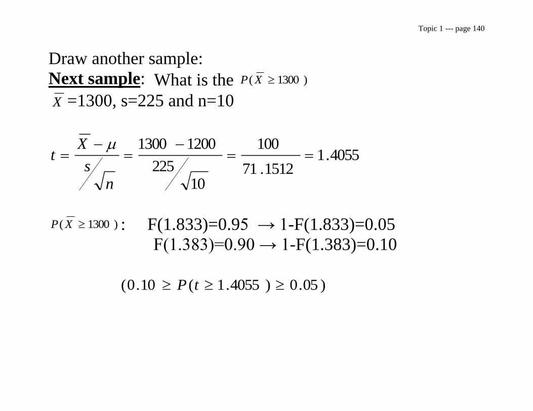
Draw another sample:
Next sample: What is the )1300( XP
X =1300, s=225 and n=10
4055.11512.71
100
10225
12001300
ns
Xt
)1300( XP : F(1.833)=0.95 → 1-F(1.833)=0.05
F(1.383)=0.90 → 1-F(1.383)=0.10
)05.0)4055.1(10.0( tP

Topic 1 --- page 141
Using EViews:
t9
0 1.4055
9.67%
t=1.383
(10% in the right tail)
t= 1.833
(5% in the right tail

Topic 1 --- page 142
Example:
Determine an interval (a,b) such that P(a t b) 0.90 ,
assuming n-1=19 degrees of freedom.
Put half of the excluded area in each tail of the distribution:
1
20 10 05
. .
t19
a 0 b
P(t b) 0.05 F(1.729) = 0.95 b = 1.729
0.05 0.05
0.95
0.90

Topic 1 --- page 143
Since the t-distribution is __________, ‘a’ is the negative
value of b:
a = -1.729.
P(-1.729 t ) 0.90 1 729.
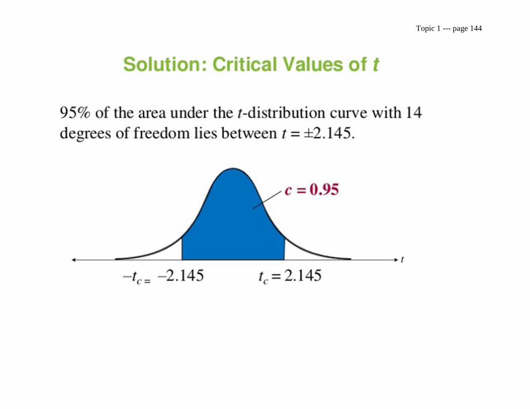
Topic 1 --- page 144
Topic 1 --- page 145
Use of the t-Distribution When the Population is Not
Normal
The discussion so far regarding the t-distribution assumes that
samples drawn are from a ________ distributed parent
population.
But often we cannot be sure or we cannot determine if the
parent population is normal.
“So how important is this normality assumption?”
The normality assumption can be ________ without
significantly changing the sampling distribution of the t-
distribution.
Topic 1 --- page 146
The distribution is said to be quite “robust”, which implies
the results still hold even if the assumptions about the parent
population do not conform to the original assumption of
normality.
We must stress that the t-distribution is appropriate
whenever ‘x’ is normal and σ is unknown, even though many
t-tables do not list values higher than ν=30.
Some texts suggest that the normal distribution be used to
approximate the t-distribution when ν > 30, since t and z-
values will then be quite close.
Because of this procedure, the t-distribution is sometimes
erroneously applied to only small samples. But, the t-
distribution is always correct whenever σ is unknown and x
is normal.
Topic 1 --- page 147
The Sampling Distribution of the Sample Variance s2,
Normal Population
We examined the sampling distribution of X to determine
how good X is as an estimator of μ.
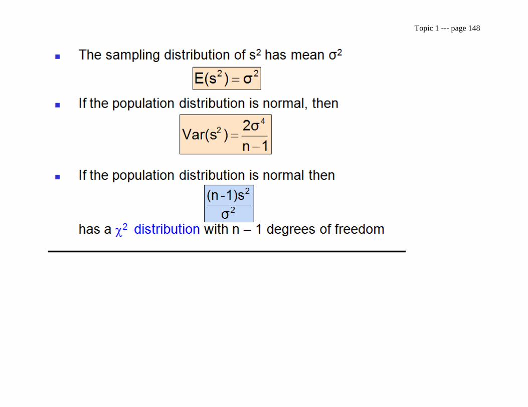
Now we need to examine the sampling distribution of s2 to
consider issues about σ2.
That is, need to explore the distribution that consists of all the
possible values of s2 calculated from samples of size n.
Topic 1 --- page 148
Topic 1 --- page 149
Characteristics of the sample variance:
1) s2 must always be _______. Hence, the distribution of s2
cannot be a normal distribution.
“s2 ” is a unimodal distribution that is _______ to the right
and looks like a smooth curve.
Sampling is from a normal population and it has one
parameter, the degree of freedom.

Topic 1 --- page 150
The shape depends on the sample _____.
2) The usual application involving s2, is analyzing whether s2
will be larger or smaller than some observed value, given
some assumed value of σ2.
f(χ2)
(χν2)
Topic 1 --- page 151
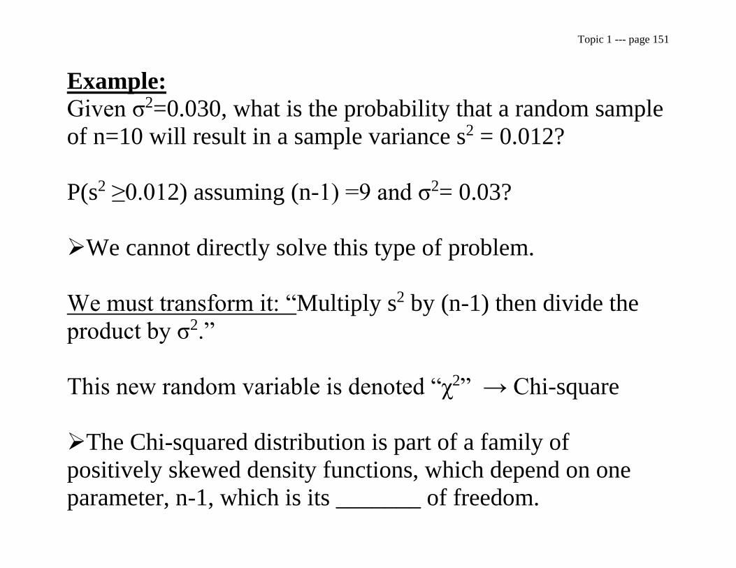
Example:
Given σ2=0.030, what is the probability that a random sample
of n=10 will result in a sample variance s2 = 0.012?
P(s2 ≥0.012) assuming (n-1) =9 and σ2= 0.03?
We cannot directly solve this type of problem.
We must transform it: “Multiply s2 by (n-1) then divide the
product by σ2.”
This new random variable is denoted “χ2” → Chi-square
The Chi-squared distribution is part of a family of
positively skewed density functions, which depend on one
parameter, n-1, which is its _______ of freedom.

Topic 1 --- page 152
n
s n s
1
2
2
2
2
2
1( ) ( )
Topic 1 --- page 153
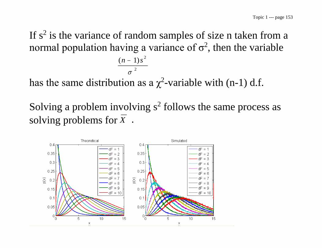
If s2 is the variance of random samples of size n taken from a
normal population having a variance of σ2, then the variable
( )n s 1
2
2
has the same distribution as a χ2-variable with (n-1) d.f.
Solving a problem involving s2 follows the same process as
solving problems for X .
Topic 1 --- page 154
Properties of 2
Distribution
1) The number of _______ of _______in a 2 distribution
determine its shape f( 2
).
When the degrees of freedom is small, the shape of the
density function is highly skewed to the ______.
As gets larger, the distribution becomes more
symmetrical.
As . The chi-square distribution becomes normal.
2) 2
is never less than zero. It has values between zero
and positive infinity.
Topic 1 --- page 155
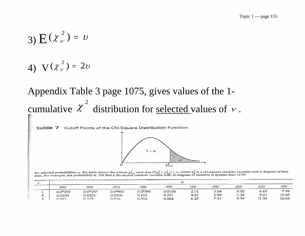
3) E ( )
2
4) V ( )
22
Appendix Table 3 page 1075, gives values of the 1-
cumulative 2
distribution for selected values of .
Topic 1 --- page 156
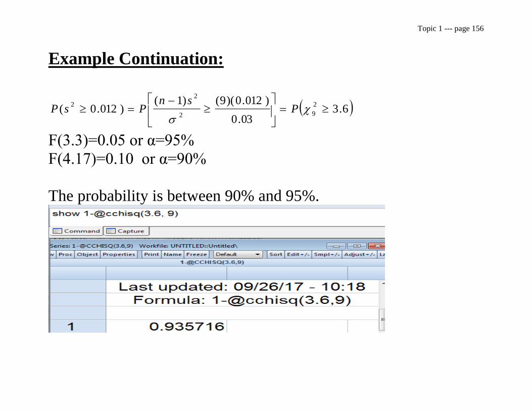
Example Continuation:
6.303.0
)012.0)(9()1()012.0(
2
92
2
2
P
snPsP
F(3.3)=0.05 or α=95%
F(4.17)=0.10 or α=90%
The probability is between 90% and 95%.

Topic 1 --- page 157
Example: Use the Chi-squared distribution to solve the
following: Assume the sample variance equals $216, s2=16,
the population variance =$29, 2 = 9,
and the sample is of size 11, n=11.
What is the probability that P s( )2
16 ?
s n s2
2
2
2
1 10 169
17 78
( ) ( )
.
From Appendix:
1-F(0.100) = 15.99
1-F(0.050) = 18.31
Meaning: 0 10 17 78 0 052
. ( . ) . P

Topic 1 --- page 158