Embed Size (px)
Citation preview
1
Reasoning Under Uncertainty
Artificial Intelligence
Chapter 9
2
ReasoningReasoning
Part 2
3
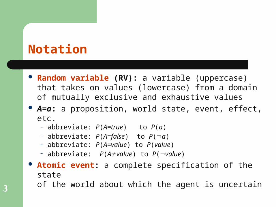
Notation
Random variable (RV): a variable (uppercase)that takes on values (lowercase) from a domainof mutually exclusive and exhaustive values
A=a: a proposition, world state, event, effect, etc.– abbreviate: P(A=true) to P(a)– abbreviate: P(A=false) to P(a)– abbreviate: P(A=value) to P(value)– abbreviate: P(Avalue) to P(value)
Atomic event: a complete specification of the stateof the world about which the agent is uncertain
4
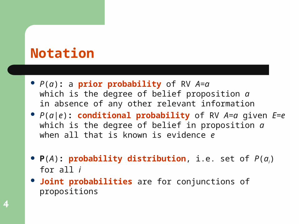
Notation
P(a): a prior probability of RV A=awhich is the degree of belief proposition ain absence of any other relevant information
P(a|e): conditional probability of RV A=a given E=ewhich is the degree of belief in proposition awhen all that is known is evidence e
P(A): probability distribution, i.e. set of P(ai) for all i Joint probabilities are for conjunctions of propositions
5
Reasoning under Uncertainty
Rather than reasoning about the truth or falsityof a proposition, instead reason about the belief that a proposition is true.
Use knowledge base of known probabilities to determine probabilities for query propositions.
6
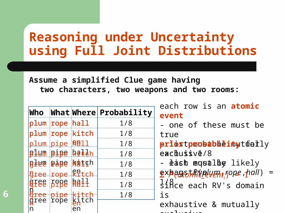
Reasoning under Uncertaintyusing Full Joint Distributions
Assume a simplified Clue game havingtwo characters, two weapons and two rooms:
each row is an atomic event- one of these must be true- list must be mutually exclusive- list must be exhaustive
Who What Whereplum rope hall
plum rope kitchen
plum pipe hall
plum pipe kitchen
green rope hall
green rope kitchen
green pipe hall
green pipe kitchen
Probability1/8
1/8
1/8
1/8
1/8
1/8
1/8
1/8
prior probability for each is 1/8- each equally likely- e.g. P(plum,rope,hall) = 1/8
hallpipeplum
kitchenpipeplum
hallropegreen
kitchenropegreen
hallpipegreen
hallropeplum
kitchenpipegreen
kitchenropeplum
P(atomic_eventi) = 1since each RV's domain isexhaustive & mutually exclusive
7
Determining Marginal Probabilitiesusing Full Joint Distributions
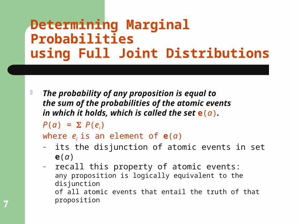
The probability of any proposition is equal tothe sum of the probabilities of the atomic eventsin which it holds, which is called the set e(a).P(a) = P(ei)where ei is an element of e(a)– its the disjunction of atomic events in set e(a)– recall this property of atomic events:
any proposition is logically equivalent to the disjunctionof all atomic events that entail the truth of that proposition
8
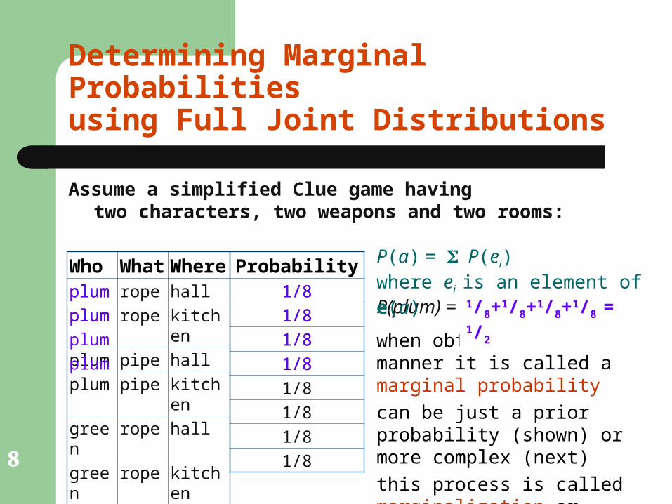
Determining Marginal Probabilitiesusing Full Joint Distributions
Assume a simplified Clue game havingtwo characters, two weapons and two rooms:
P(plum) = ?
Who What Whereplum rope hall
plum rope kitchen
plum pipe hall
plum pipe kitchen
green rope hall
green rope kitchen
green pipe hall
green pipe kitchen
Probability1/8
1/8
1/8
1/8
1/8
1/8
1/8
1/8
when obtained in this manner it is called a marginal probability
can be just a prior probability (shown) or more complex (next)
this process is called marginalization or summing out
1/8+1/8+1/8+1/8 = 1/2
1/8
1/8
1/8
1/8
P(a) = P(ei)where ei is an element of e(a)
plum
plum
plum
plum
9
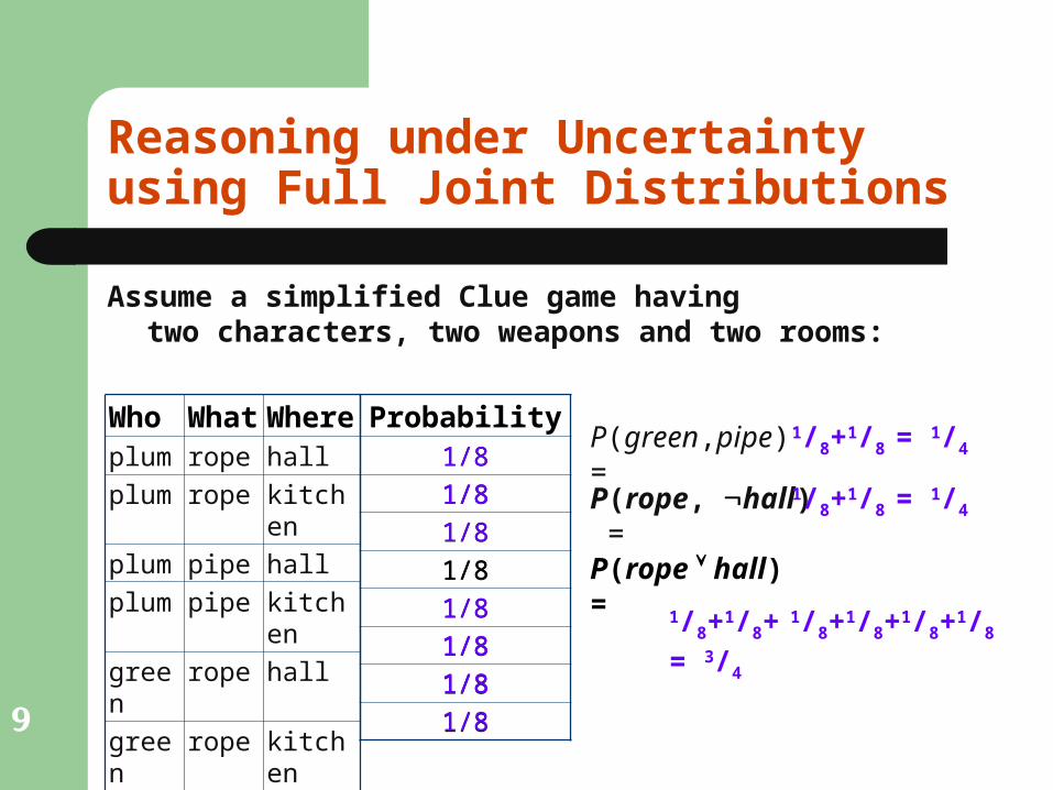
Reasoning under Uncertaintyusing Full Joint Distributions
Assume a simplified Clue game havingtwo characters, two weapons and two rooms:
P(green,pipe) =
Who What Whereplum rope hall
plum rope kitchen
plum pipe hall
plum pipe kitchen
green rope hall
green rope kitchen
green pipe hall
green pipe kitchen
Probability1/8
1/8
1/8
1/8
1/8
1/8
1/8
1/8
1/8+1/8 = 1/4
1/8
1/8
1/8
P(rope, hall) =
1/8
1/8 1/8+1/8 = 1/4
P(rope hall) = 1/8+1/8+
1/8+1/8+1/8+1/8 = 3/4
1/8
1/8
1/8
1/8
1/8
1/8
10
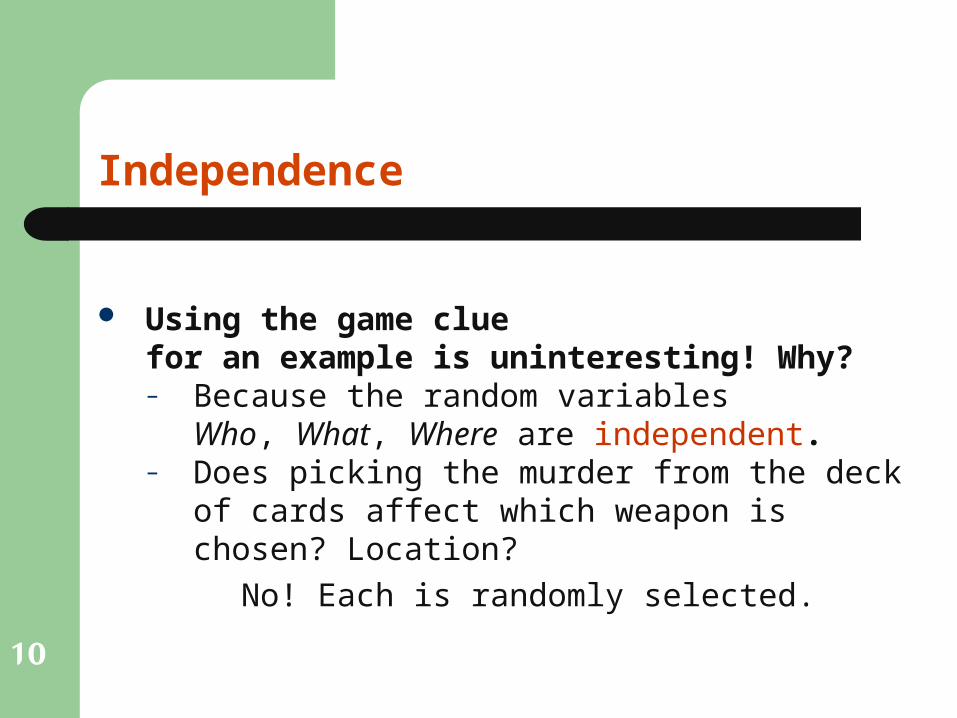
Independence
Using the game cluefor an example is uninteresting! Why?– Because the random variables
Who, What, Where are independent.– Does picking the murder from the deck of cards
affect which weapon is chosen? Location?
No! Each is randomly selected.
11
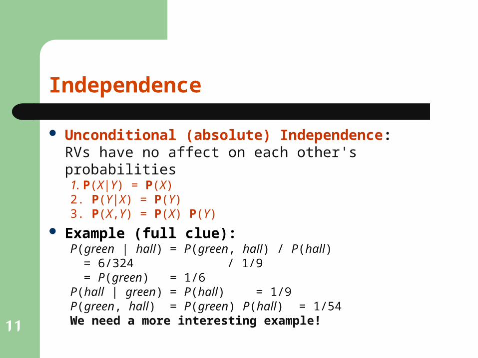
Independence
Unconditional (absolute) Independence:RVs have no affect on each other's probabilities1. P(X|Y) = P(X)2. P(Y|X) = P(Y)3. P(X,Y) = P(X) P(Y)
Example (full clue):P(green | hall) = P(green, hall) / P(hall)
= 6/324 / 1/9= P(green) = 1/6
P(hall | green) = P(hall) = 1/9P(green, hall) = P(green) P(hall) = 1/54We need a more interesting example!
12
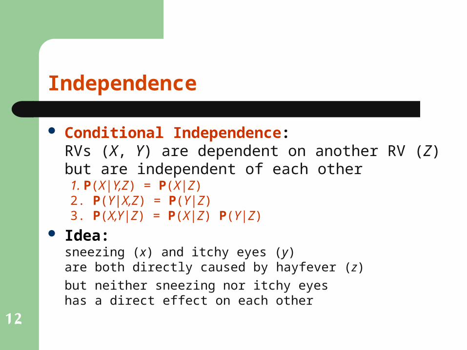
Independence
Conditional Independence:RVs (X, Y) are dependent on another RV (Z)but are independent of each other1. P(X|Y,Z) = P(X|Z)2. P(Y|X,Z) = P(Y|Z) 3. P(X,Y|Z) = P(X|Z) P(Y|Z)
Idea:sneezing (x) and itchy eyes (y)are both directly caused by hayfever (z)
but neither sneezing nor itchy eyeshas a direct effect on each other
13
HF SN IEfalse false false
false false true
false true false
false true true
true false false
true false true
true true false
true true true
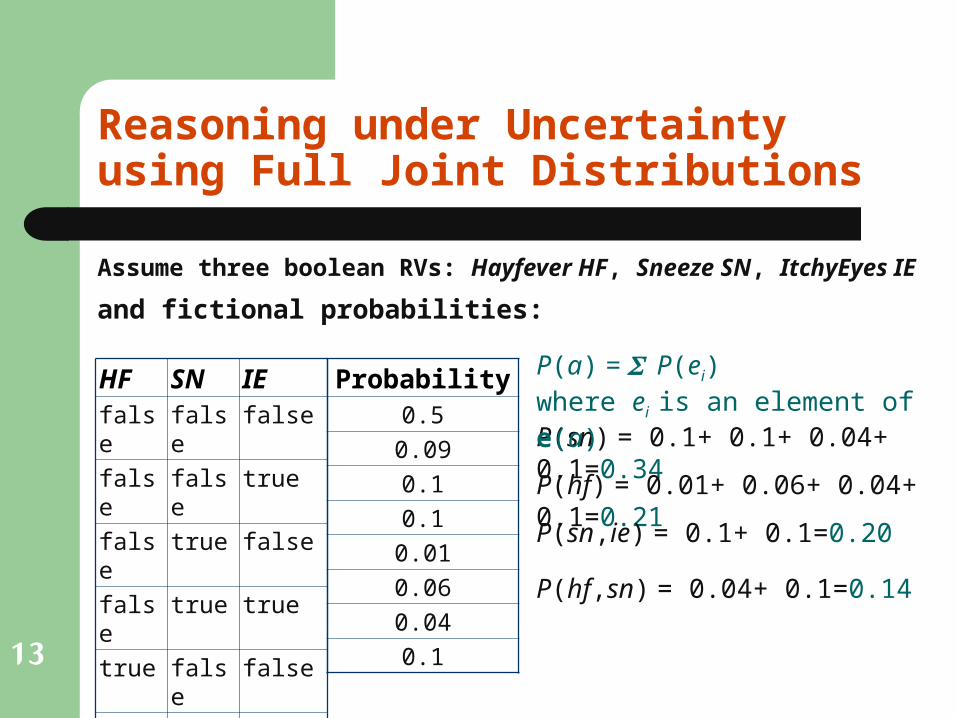
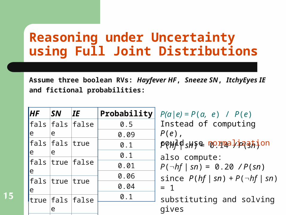
Reasoning under Uncertaintyusing Full Joint Distributions
Assume three boolean RVs: Hayfever HF, Sneeze SN, ItchyEyes IE
P(sn) = 0.1+ 0.1+ 0.04+ 0.1=0.34
Probability0.5
0.09
0.1
0.1
0.01
0.06
0.04
0.1
P(a) = P(ei)where ei is an element of e(a)
P(hf) = 0.01+ 0.06+ 0.04+ 0.1=0.21P(sn,ie) = 0.1+ 0.1=0.20
P(hf,sn) = 0.04+ 0.1=0.14
and fictional probabilities:
14
HF SN IEfalse false false
false false true
false true false
false true true
true false false
true false true
true true false
true true true
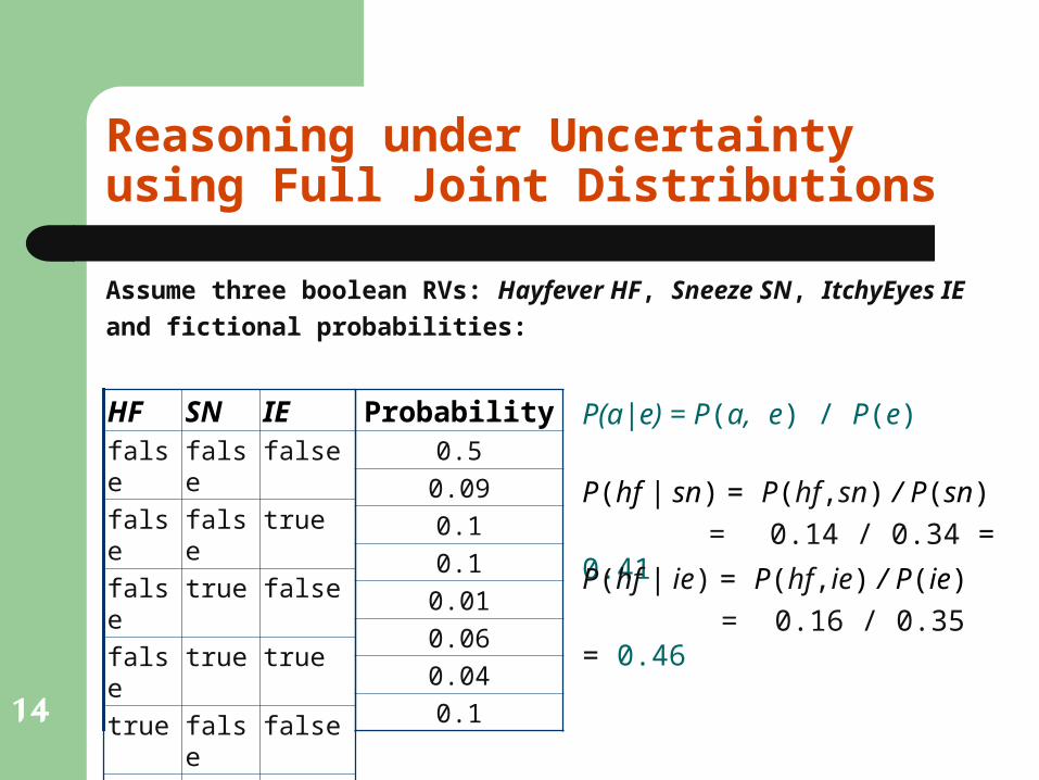
Reasoning under Uncertaintyusing Full Joint Distributions
Assume three boolean RVs: Hayfever HF, Sneeze SN, ItchyEyes IEand fictional probabilities:
Probability0.5
0.09
0.1
0.1
0.01
0.06
0.04
0.1
P(a|e) = P(a, e) / P(e)
P(hf | sn) = P(hf,sn) / P(sn) = 0.14 / 0.34 =
0.41P(hf | ie) = P(hf,ie) / P(ie) = 0.16 / 0.35 =
0.46
15
HF SN IEfalse false false
false false true
false true false
false true true
true false false
true false true
true true false
true true true
Reasoning under Uncertaintyusing Full Joint Distributions
Assume three boolean RVs: Hayfever HF, Sneeze SN, ItchyEyes IEand fictional probabilities:
P(hf | sn) = 0.14 / P(sn)
Probability0.5
0.09
0.1
0.1
0.01
0.06
0.04
0.1
Instead of computing P(e),could use normalization
also compute:P(hf | sn) = 0.20 / P(sn)since P(hf | sn) + P(hf | sn) = 1substituting and solving gives
P(sn) = 0.34 !
P(a|e) = P(a, e) / P(e)
16
Combining Multiple Evidence
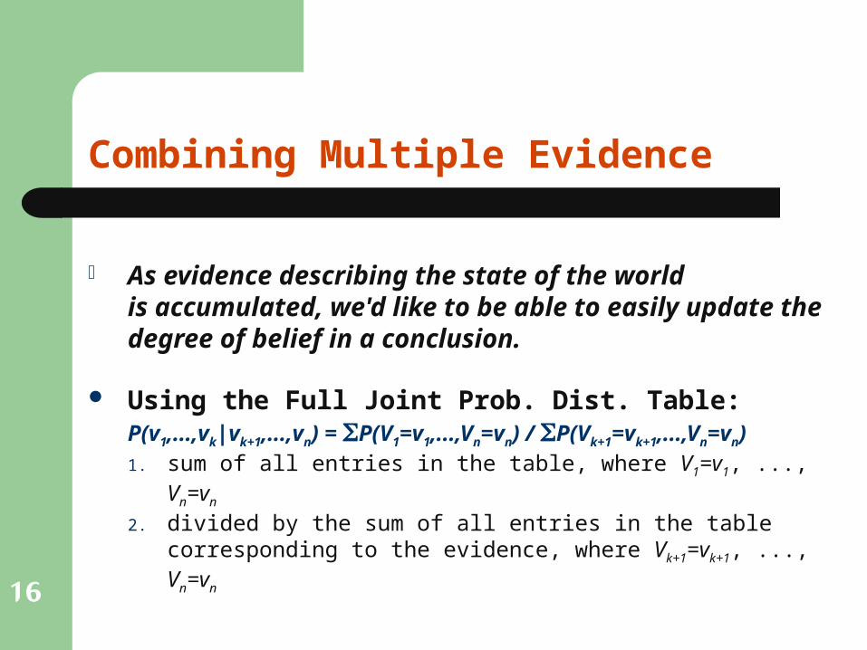
As evidence describing the state of the worldis accumulated, we'd like to be able to easily update the degree of belief in a conclusion.
Using the Full Joint Prob. Dist. Table:P(v1,...,vk|vk+1,...,vn) = P(V1=v1,...,Vn=vn) /
P(Vk+1=vk+1,...,Vn=vn)1. sum of all entries in the table, where V1=v1, ..., Vn=vn
2. divided by the sum of all entries in the tablecorresponding to the evidence, where Vk+1=vk+1, ..., Vn=vn
17
HF SN IEfalse false false
false false true
false true false
false true true
true false false
true false true
true true false
true true true
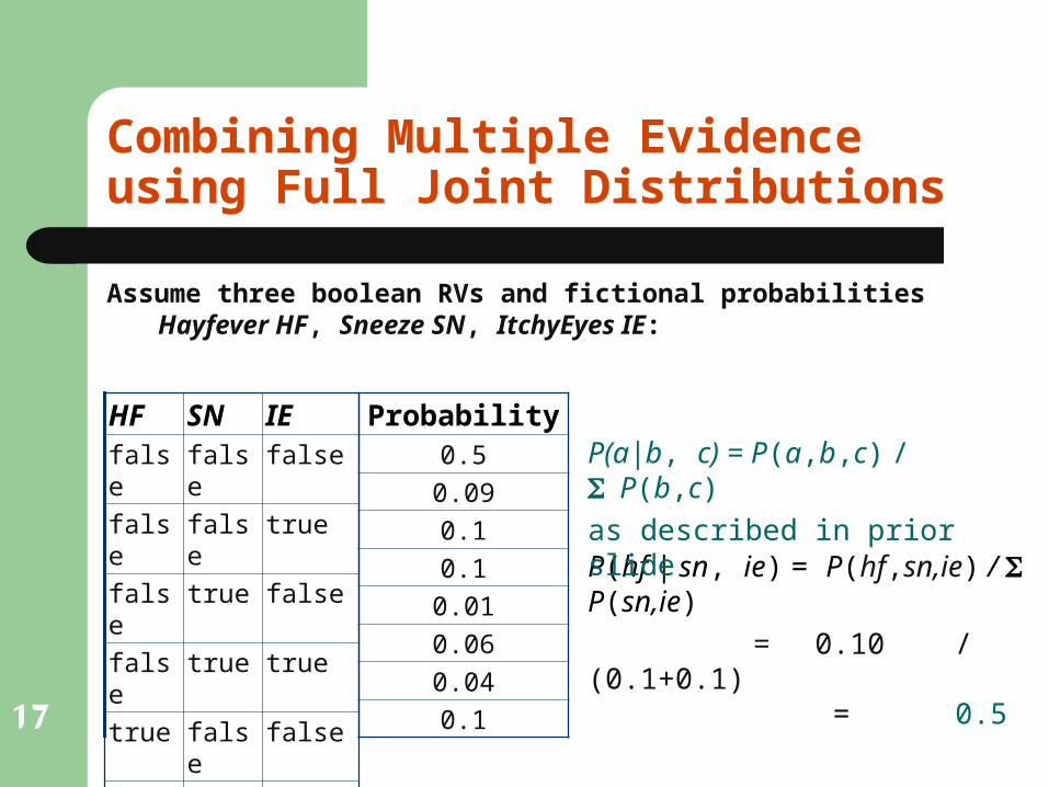
Combining Multiple Evidenceusing Full Joint Distributions
Assume three boolean RVs and fictional probabilities Hayfever HF, Sneeze SN, ItchyEyes IE:
P(hf | sn, ie) = P(hf,sn,ie) / P(sn,ie)
= 0.10 / (0.1+0.1)
= 0.5
Probability0.5
0.09
0.1
0.1
0.01
0.06
0.04
0.1
P(a|b, c) = P(a,b,c) / P(b,c) as described in prior slide
18
Combining Multiple Evidence (cont.)
FJDT techniques are intractable in general because the table size grows exponentially.
Independence assertions can help reducethe size of the domain and the complexityof the inference problem.
Independence assertions are usually basedon the knowledge of the domain enablingFJD table to be factored in to separate JD tables.– it's a good thing that problem domains are independent– but typically subsets of dependent RVs are quite large
19
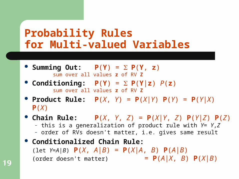
Probability Rulesfor Multi-valued Variables
Summing Out: P(Y) = P(Y, z)sum over all values z of RV Z
Conditioning: P(Y) = P(Y|z) P(z)sum over all values z of RV Z
Product Rule: P(X, Y) = P(X|Y) P(Y) = P(Y|X) P(X) Chain Rule: P(X, Y, Z) = P(X|Y, Z) P(Y|Z) P(Z)
– this is a generalization of product rule with Y= Y,Z– order of RVs doesn't matter, i.e. gives same result
Conditionalized Chain Rule:(let Y=A|B) P(X, A|B) = P(X|A, B) P(A|B)(order doesn't matter) = P(A|X, B) P(X|B)
20
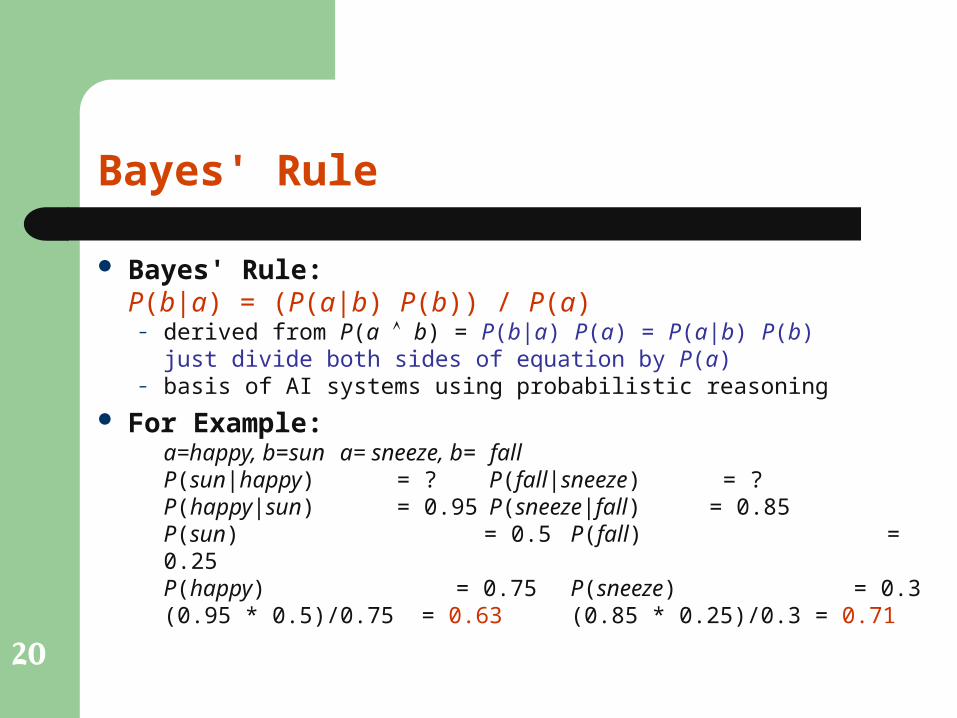
Bayes' Rule
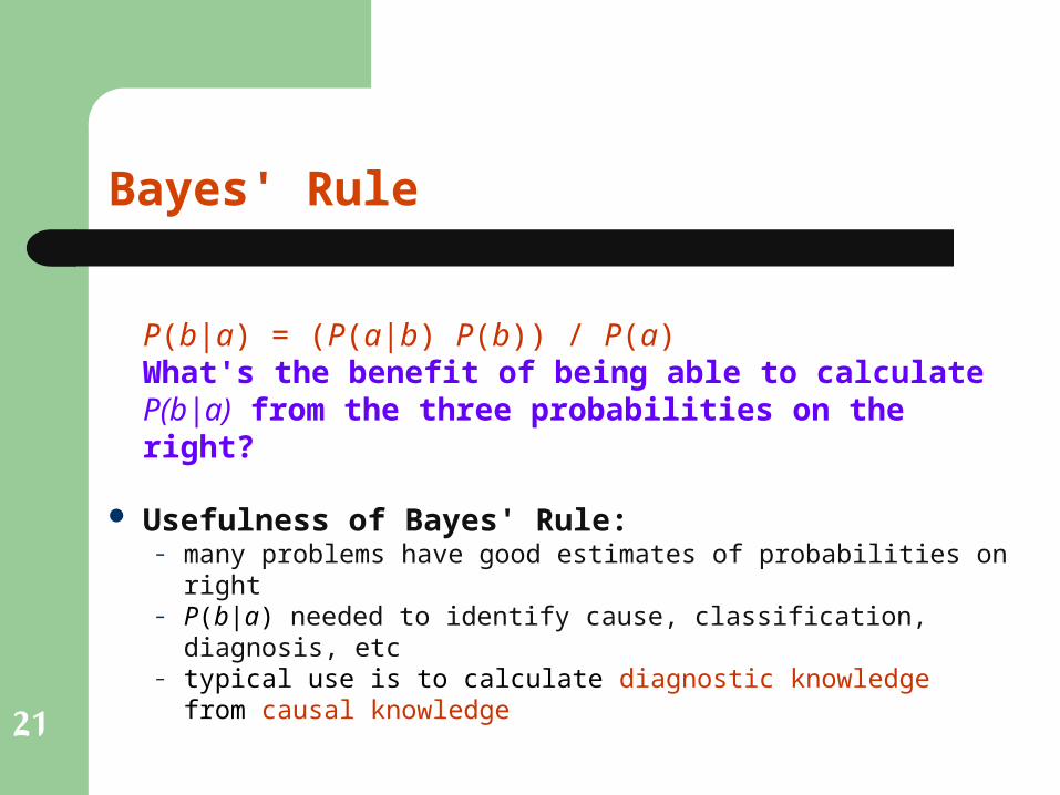
Bayes' Rule:P(b|a) = (P(a|b) P(b)) / P(a)
– derived from P(a b) = P(b|a) P(a) = P(a|b) P(b)just divide both sides of equation by P(a)
– basis of AI systems using probabilistic reasoning
For Example:a=happy, b=sun a= sneeze, b= fallP(sun|happy) = ? P(fall|sneeze) = ?P(happy|sun) = 0.95 P(sneeze|fall) = 0.85P(sun) = 0.5 P(fall) = 0.25P(happy) = 0.75 P(sneeze) = 0.3(0.95 * 0.5)/0.75 = 0.63 (0.85 * 0.25)/0.3 = 0.71
21
Bayes' Rule
P(b|a) = (P(a|b) P(b)) / P(a)What's the benefit of being able to calculateP(b|a) from the three probabilities on the right?
Usefulness of Bayes' Rule:– many problems have good estimates of probabilities on right– P(b|a) needed to identify cause, classification, diagnosis, etc– typical use is to calculate diagnostic knowledge
from causal knowledge
22
Bayes' Rule
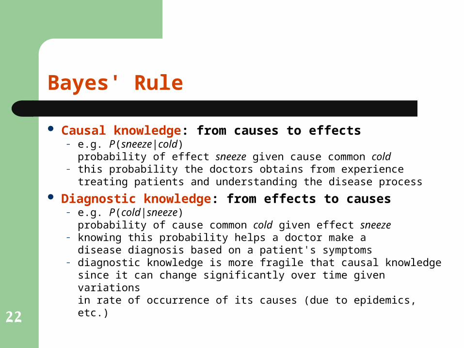
Causal knowledge: from causes to effects– e.g. P(sneeze|cold)
probability of effect sneeze given cause common cold– this probability the doctors obtains from experience
treating patients and understanding the disease process
Diagnostic knowledge: from effects to causes– e.g. P(cold|sneeze)
probability of cause common cold given effect sneeze– knowing this probability helps a doctor make a
disease diagnosis based on a patient's symptoms– diagnostic knowledge is more fragile that causal knowledge
since it can change significantly over time given variationsin rate of occurrence of its causes (due to epidemics, etc.)
23
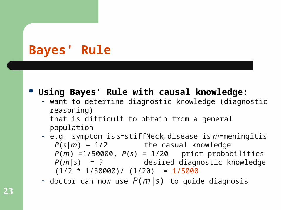
Bayes' Rule
Using Bayes' Rule with causal knowledge:– want to determine diagnostic knowledge (diagnostic reasoning)
that is difficult to obtain from a general population– e.g. symptom is s=stiffNeck, disease is m=meningitis
P(s|m) = 1/2 the casual knowledgeP(m) =1/50000, P(s) = 1/20 prior probabilitiesP(m|s) = ? desired diagnostic knowledge(1/2 * 1/50000)/ (1/20) = 1/5000
– doctor can now use P(m|s) to guide diagnosis
24
Combining Multiple Evidenceusing Bayes' Rule
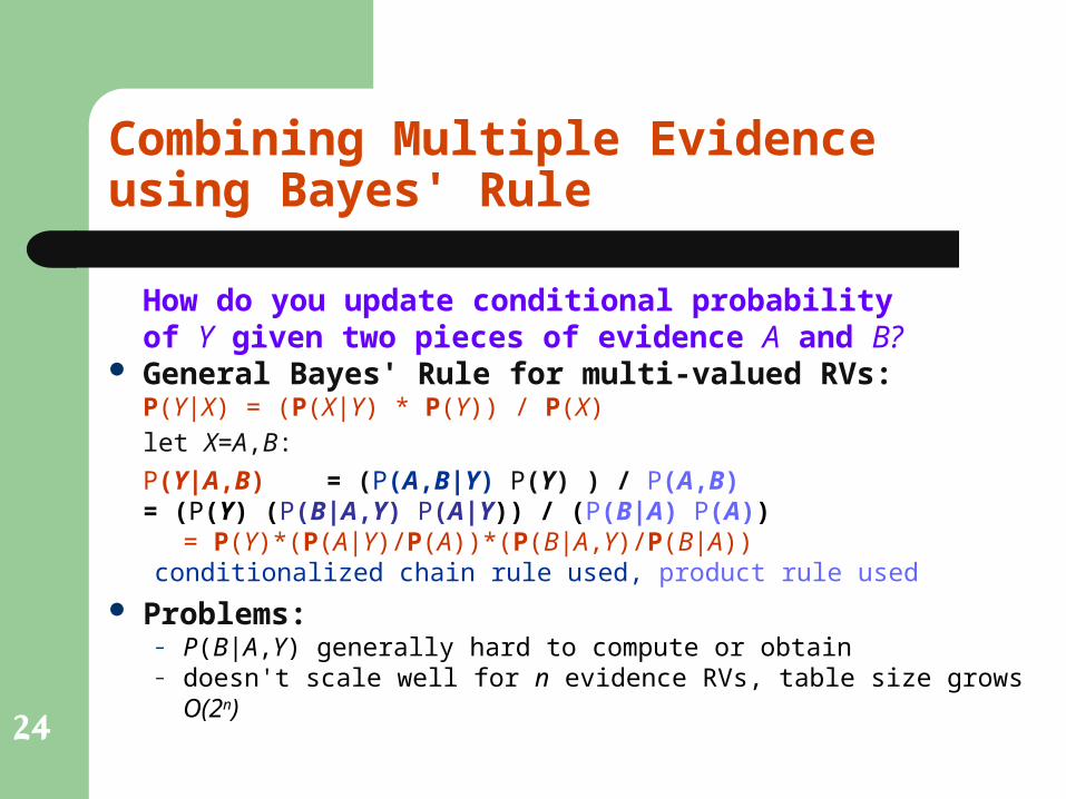
How do you update conditional probabilityof Y given two pieces of evidence A and B?
General Bayes' Rule for multi-valued RVs:P(Y|X) = (P(X|Y) * P(Y)) / P(X)let X=A,B:
P(Y|A,B) = (P(A,B|Y) P(Y) ) / P(A,B)= (P(Y) (P(B|A,Y) P(A|Y)) / (P(B|A) P(A))
= P(Y)*(P(A|Y)/P(A))*(P(B|A,Y)/P(B|A))conditionalized chain rule used, product rule used
Problems:– P(B|A,Y) generally hard to compute or obtain– doesn't scale well for n evidence RVs, table size grows O(2n)
25
Combining Multiple Evidenceusing Bayes' Rule
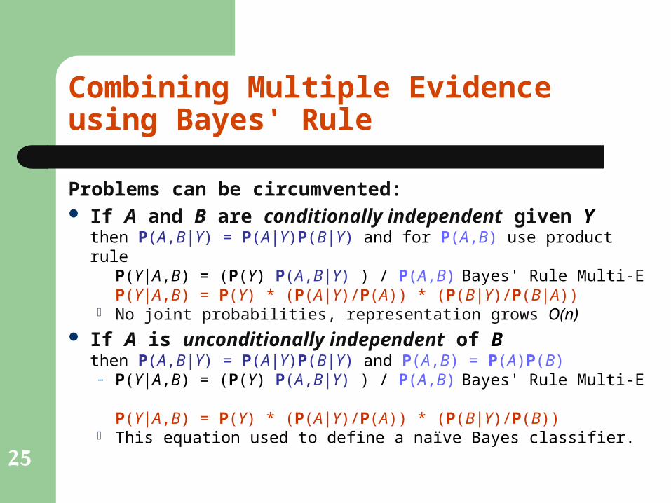
Problems can be circumvented: If A and B are conditionally independent given Y
then P(A,B|Y) = P(A|Y)P(B|Y) and for P(A,B) use product rule P(Y|A,B) = (P(Y) P(A,B|Y) ) / P(A,B)Bayes' Rule Multi-EP(Y|A,B) = P(Y) * (P(A|Y)/P(A)) * (P(B|Y)/P(B|A))
No joint probabilities, representation grows O(n) If A is unconditionally independent of B
then P(A,B|Y) = P(A|Y)P(B|Y) and P(A,B) = P(A)P(B)– P(Y|A,B) = (P(Y) P(A,B|Y) ) / P(A,B)Bayes' Rule Multi-E
P(Y|A,B) = P(Y) * (P(A|Y)/P(A)) * (P(B|Y)/P(B)) This equation used to define a naïve Bayes classifier.
26
Combining Multiple Evidenceusing Bayes' Rule
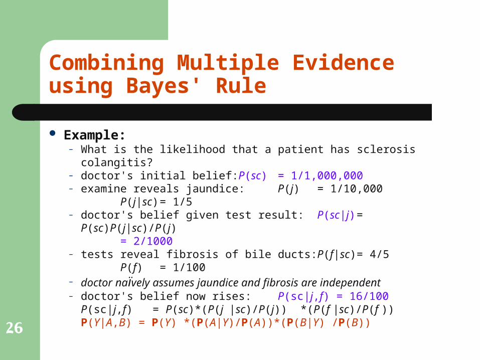
Example:– What is the likelihood that a patient has sclerosis colangitis?– doctor's initial belief: P(sc) = 1/1,000,000– examine reveals jaundice: P(j) = 1/10,000
P(j|sc) = 1/5– doctor's belief given test result: P(sc|j) = P(sc)P(j|sc)/P(j)
= 2/1000– tests reveal fibrosis of bile ducts: P(f|sc) = 4/5
P(f) = 1/100– doctor naïvely assumes jaundice and fibrosis are independent– doctor's belief now rises: P(sc|j,f) = 16/100
P(sc|j,f) = P(sc)*(P(j |sc)/P(j)) *(P(f |sc)/P(f )) P(Y|A,B) = P(Y) *(P(A|Y)/P(A))*(P(B|Y) /P(B))
27
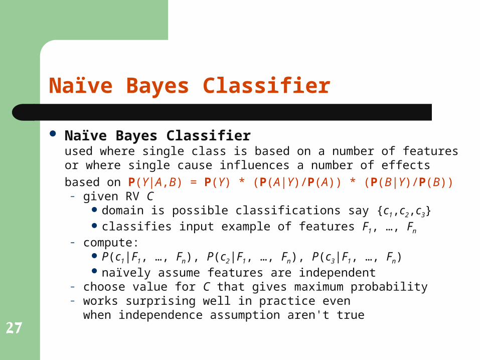
Naïve Bayes Classifier
Naïve Bayes Classifierused where single class is based on a number of featuresor where single cause influences a number of effects
based on P(Y|A,B) = P(Y) * (P(A|Y)/P(A)) * (P(B|Y)/P(B))– given RV C
domain is possible classifications say {c1,c2,c3} classifies input example of features F1, …, Fn
– compute: P(c1|F1, …, Fn), P(c2|F1, …, Fn), P(c3|F1, …, Fn) naïvely assume features are independent
– choose value for C that gives maximum probability– works surprising well in practice even
when independence assumption aren't true
28
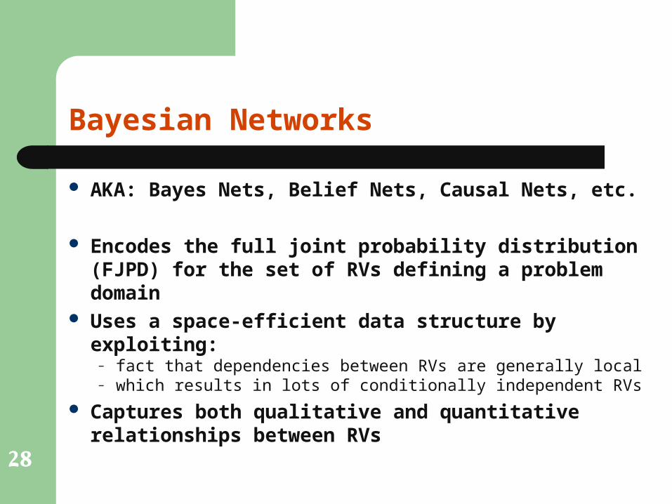
Bayesian Networks
AKA: Bayes Nets, Belief Nets, Causal Nets, etc.
Encodes the full joint probability distribution (FJPD) for the set of RVs defining a problem domain
Uses a space-efficient data structure by exploiting:– fact that dependencies between RVs are generally local– which results in lots of conditionally independent RVs
Captures both qualitative and quantitative relationships between RVs
29
Bayesian Networks
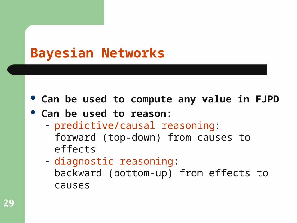
Can be used to compute any value in FJPD Can be used to reason:
– predictive/causal reasoning:forward (top-down) from causes to effects
– diagnostic reasoning:backward (bottom-up) from effects to causes
30
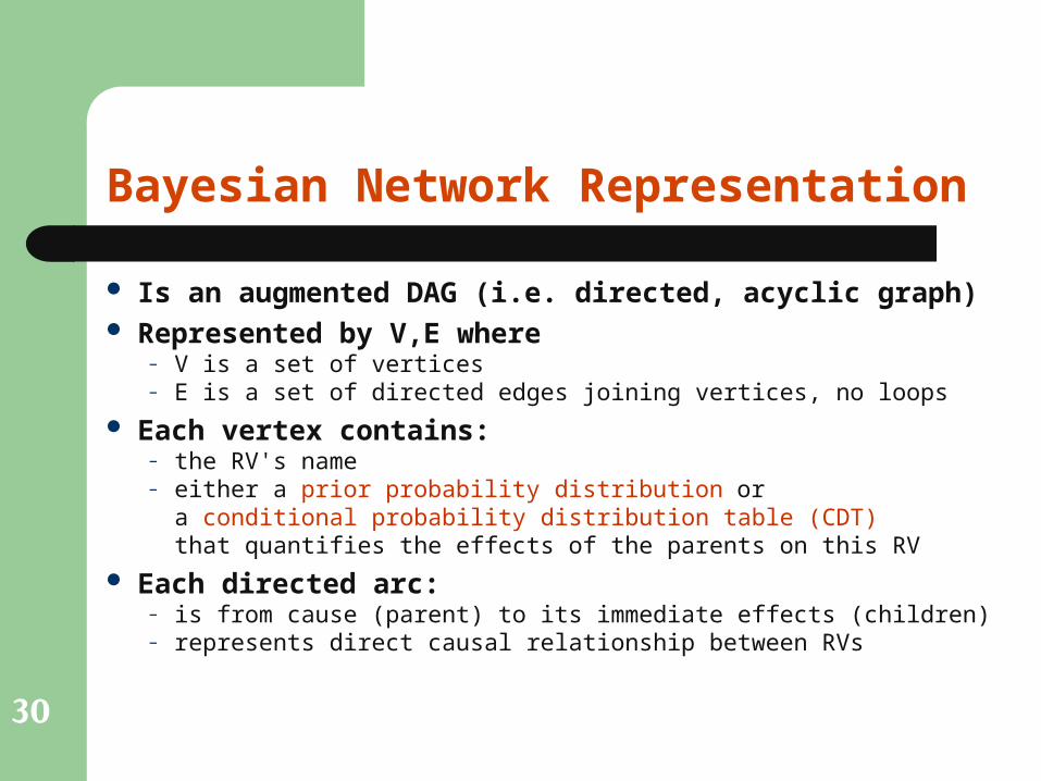
Bayesian Network Representation
Is an augmented DAG (i.e. directed, acyclic graph) Represented by V,E where
– V is a set of vertices– E is a set of directed edges joining vertices, no loops
Each vertex contains:– the RV's name– either a prior probability distribution or
a conditional probability distribution table (CDT)that quantifies the effects of the parents on this RV
Each directed arc:– is from cause (parent) to its immediate effects (children)– represents direct causal relationship between RVs
31
Bayesian Network Representation
Example: in class– each row in conditional probability tables must sum to 1– columns don't need to sum to 1– values obtained from experts
Number of probabilities required is typicallyfar fewer than the number required for a FJDT
Quantitative information is usually givenby an expert or determined empirically from data
32
Conditional Independence
Assume effects are conditionally independentof each other given their common cause
The net is constructed so that given its parents,a node is conditionally independent of its non-descendant RVs in the net:P(X1=x1, ..., Xn=xn) = P(xi | parents(Xi)) * ... * P(xn | parents(Xn))
Note the full joint probability distribution isn't needed, only need conditionals relative to their parent RVs
33
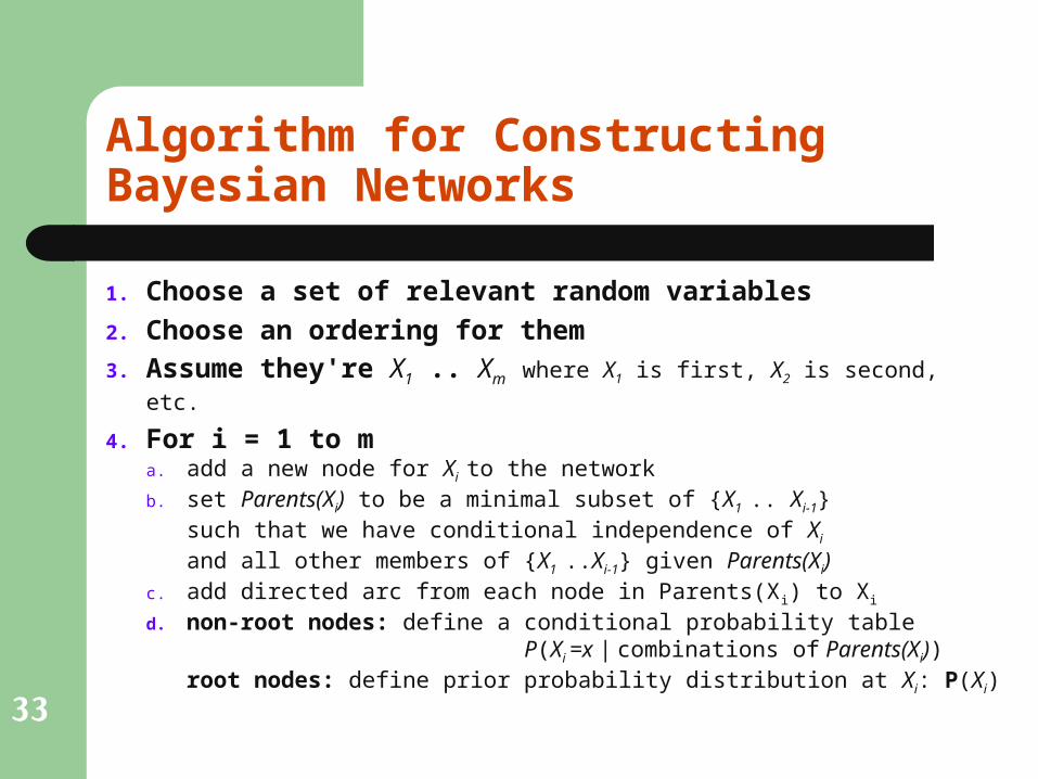
Algorithm for ConstructingBayesian Networks
1. Choose a set of relevant random variables
2. Choose an ordering for them
3. Assume they're X1 .. Xm where X1 is first, X2 is second, etc.
4. For i = 1 to ma. add a new node for Xi to the networkb. set Parents(Xi) to be a minimal subset of {X1 .. Xi-1}
such that we have conditional independence of Xi
and all other members of {X1 ..Xi-1} given Parents(Xi)c. add directed arc from each node in Parents(X i) to Xi d. non-root nodes: define a conditional probability table
P(Xi =x | combinations of Parents(Xi)) root nodes: define prior probability distribution at Xi: P(Xi)
34
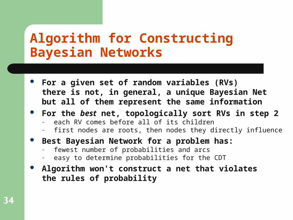
Algorithm for ConstructingBayesian Networks
For a given set of random variables (RVs)there is not, in general, a unique Bayesian Netbut all of them represent the same information
For the best net, topologically sort RVs in step 2– each RV comes before all of its children– first nodes are roots, then nodes they directly influence
Best Bayesian Network for a problem has:– fewest number of probabilities and arcs– easy to determine probabilities for the CDT
Algorithm won't construct a net that violatesthe rules of probability

35
Compute P(a,b,c,d) = P(d,c,b,a)order RVS in joint probability bottom up D,C,B,A= P(d|c,b,a) P(c,b,a) Product Rule P(d,c,b,a) = P(d|c) P(c,b,a) Conditional Independ. of D given C= P(d|c) P(c|b,a) P(b,a) Product Rule P(c,b,a) = P(d|c) P(c|b,a) P(b|a) P(a) Product Rule P(b,a) = P(d|c) P(c|b,a) P(b ) P(a) Independence of B and A
given no evidence
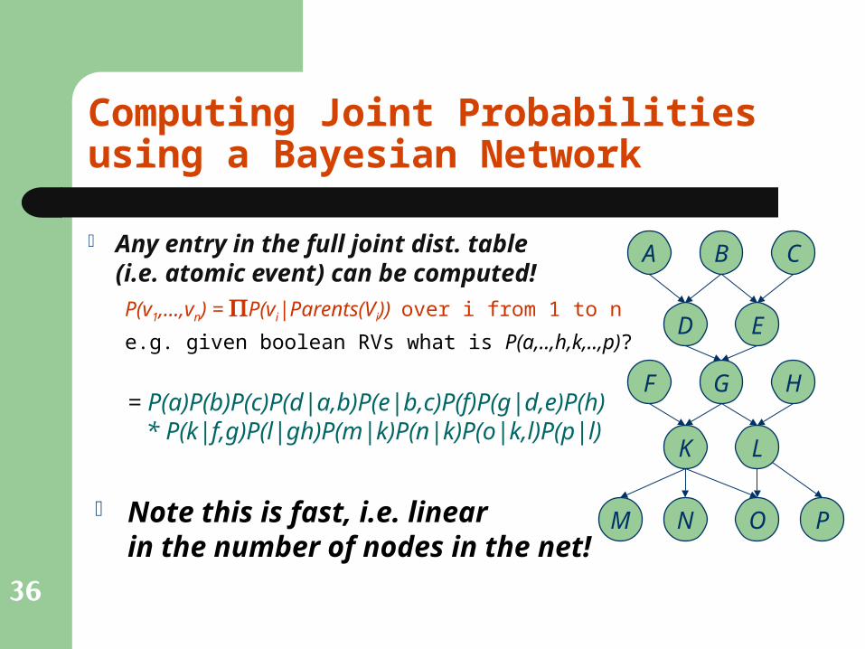
Computing Joint Probabilitiesusing a Bayesian Network
1. Use product rule
2. Simplify using independence
For Example:
A B
C
D
36
Computing Joint Probabilitiesusing a Bayesian Network
Any entry in the full joint dist. table(i.e. atomic event) can be computed!
P(v1,...,vn) = P(vi|Parents(Vi)) over i from 1 to n
e.g. given boolean RVs what is P(a,..,h,k,..,p)?D E
G
A
K
B
HF
C
L
N O PM
= P(a)P(b)P(c)P(d|a,b)P(e|b,c)P(f)P(g|d,e)P(h) * P(k|f,g)P(l|gh)P(m|k)P(n|k)P(o|k,l)P(p|l)
Note this is fast, i.e. linearin the number of nodes in the net!
37
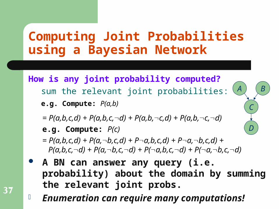
Computing Joint Probabilitiesusing a Bayesian Network
How is any joint probability computed?
sum the relevant joint probabilities:
e.g. Compute: P(a,b)
= P(a,b,c,d) + P(a,b,c,d) + P(a,b,c,d) + P(a,b,c,d)e.g. Compute: P(c)= P(a,b,c,d) + P(a,b,c,d) + Pa,b,c,d) + Pa,b,c,d) + P(a,b,c,d) + P(a,b,c,d) + P(a,b,c,d) + P(a,b,c,d)
A BN can answer any query (i.e. probability) about the domain by summing the relevant joint probs.
Enumeration can require many computations!
A B
C
D
38
Computing Conditional Probabilitiesusing a Bayesian Network
Basic task of probabilistic systemis to compute conditional probabilities.
Any conditional probability can be computed:P(v1,...,vk|vk+1,...,vn) = P(V1=v1,...,Vn=vn) /
P(Vk+1=vk+1,...,Vn=vn)
Key problem is that the technique of enumeratingjoint probabilities can make the computations intractable (exponential in the number of RVs).
39
Computing Conditional Probabilitiesusing a Bayesian Network
These computations generally relyon the simplifications resulting fromthe independence of the RVs.
Every variable that isn't an ancestorof a query variable or an evidence variableis irrelevant to the query.
What ancestors are irrelevant?
40
D E
G
A
K
B
HF
C
L
N O PM
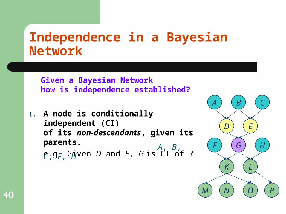
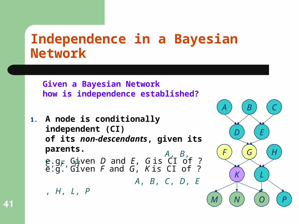
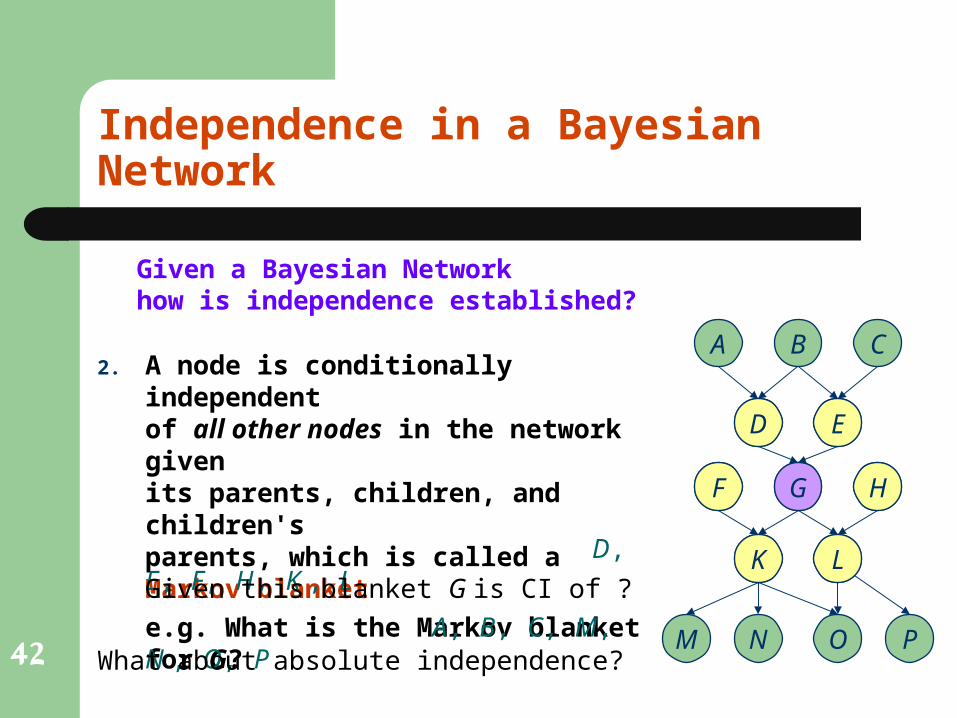
Independence in a Bayesian Network
Given a Bayesian Networkhow is independence established?
1. A node is conditionally independent (CI)of its non-descendants, given its parents.
e.g. Given D and E, G is CI of ?G
D E
A, B, C, F, H
A B
HF
C
41
D E
G
A
K
B
HF
C
L
N O PM
Independence in a Bayesian Network
Given a Bayesian Networkhow is independence established?
1. A node is conditionally independent (CI)of its non-descendants, given its parents.
e.g. Given D and E, G is CI of ?
A, B, C, F, He.g. Given F and G, K is CI of ?
GF
KA, B, C, D, E ,
H, L, P
D E
A B
H
C
L
P
42
D E
G
A
K
B
HF
C
L
N O PM
Independence in a Bayesian Network
Given a Bayesian Networkhow is independence established?
2. A node is conditionally independentof all other nodes in the network givenits parents, children, and children'sparents, which is called a Markov blanket
e.g. What is the Markov blanket for G? G
D E
K
HF
L D, E, F, H, K , LGiven this blanket G is CI of ?
A, B, C, M, N , O, PWhat about absolute independence?
43
Computing Conditional Probabilitiesusing a Bayesian Network
The general algorithm for computingconditional probabilities is complicated.
It is easy if the query involves nodesthat are directly connected to each other.examples assumed to use boolean RVs
Simple causal inference: P(E|C)– conditional prob. dist. of effect E given cause C as evidence– reasoning in same direction as arc, e.g. disease to symptom
Simple diagnostic inference: P(Q|E)– conditional prob. dist. of query Q given effect E as evidence– reasoning in direction opposite of arc, e.g. symptom to disease
44
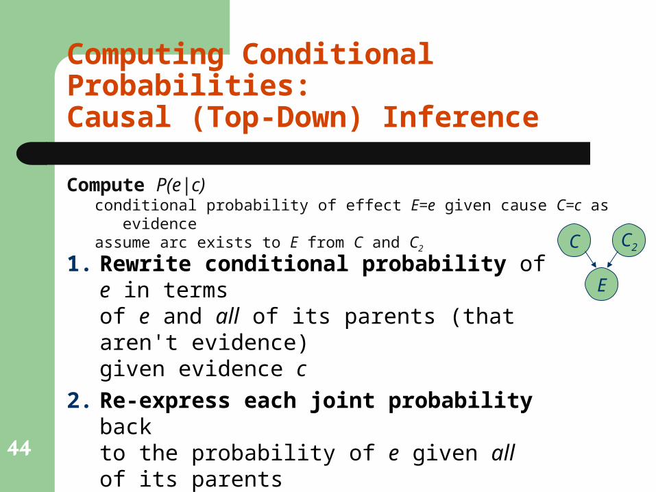
Computing Conditional Probabilities:Causal (Top-Down) Inference
Compute P(e|c)conditional probability of effect E=e given cause C=c as evidenceassume arc exists to E from C and C2 C C2
E1. Rewrite conditional probability of e in terms
of e and all of its parents (that aren't evidence)given evidence c
2. Re-express each joint probability backto the probability of e given all of its parents
3. Simplify using independence and Look Uprequired values in the Bayesian Network
45
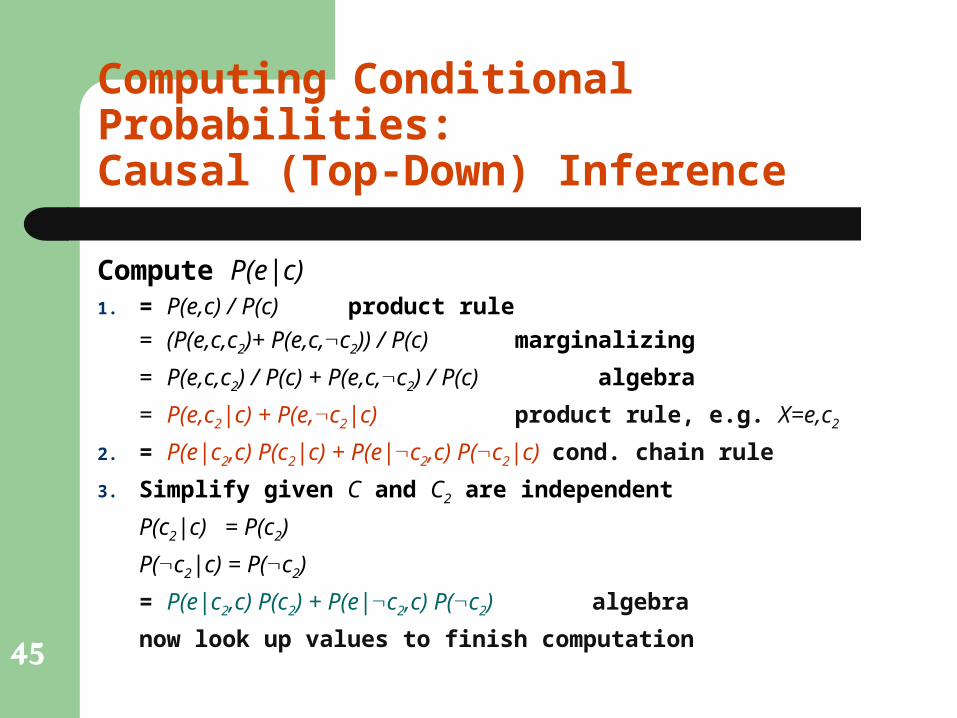
Computing Conditional Probabilities:Causal (Top-Down) Inference
Compute P(e|c)1. = P(e,c) / P(c) product rule
= (P(e,c,c2)+ P(e,c,c2)) / P(c) marginalizing
= P(e,c,c2) / P(c) + P(e,c,c2) / P(c) algebra
= P(e,c2|c) + P(e,c2|c) product rule, e.g. X=e,c2
2. = P(e|c2,c) P(c2|c) + P(e|c2,c) P(c2|c) cond. chain rule
3. Simplify given C and C2 are independent
P(c2|c) = P(c2)
P(c2|c) = P(c2)
= P(e|c2,c) P(c2) + P(e|c2,c) P(c2) algebra
now look up values to finish computation
46
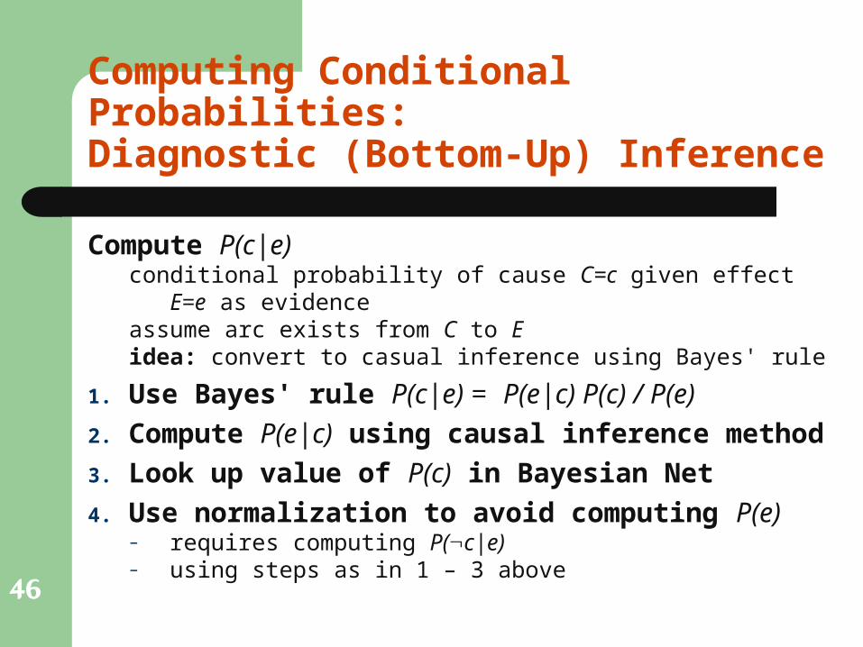
Computing Conditional Probabilities:Diagnostic (Bottom-Up) Inference
Compute P(c|e)conditional probability of cause C=c given effect E=e as
evidenceassume arc exists from C to Eidea: convert to casual inference using Bayes' rule
1. Use Bayes' rule P(c|e) = P(e|c) P(c) / P(e)2. Compute P(e|c) using causal inference method
3. Look up value of P(c) in Bayesian Net
4. Use normalization to avoid computing P(e)– requires computing P(c|e)– using steps as in 1 – 3 above
47
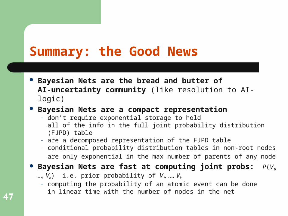
Summary: the Good News
Bayesian Nets are the bread and butter ofAI-uncertainty community (like resolution to AI-logic)
Bayesian Nets are a compact representation– don't require exponential storage to hold
all of the info in the full joint probability distribution (FJPD) table– are a decomposed representation of the FJPD table– conditional probability distribution tables in non-root nodes are
only exponential in the max number of parents of any node Bayesian Nets are fast at computing joint probs:
P(V1, ..., Vk) i.e. prior probability of V1, ..., Vk
– computing the probability of an atomic event can be donein linear time with the number of nodes in the net
48
Summary: the Bad News
Conditional probabilities can also be computed:P(Q|E1, ..., Ek)posterior probability of query Q given multiple evidence E1, ..., Ek
– requires enumerating all of the matching entries,which takes exponential time in the number of variables
– in special cases it can be done faster, <= polynomial timee.g. polytree: linear time for nets structured like trees
In general, inference in Bayesian Networks (BN)is NP-hard. but BNs are well studied so there exists many efficient exact solution methods as well as a variety of approximation techniques