1

Research Methods

Winter 2008Winter 2008

Review for Test 1Review for Test 1 Chapter s 1- 4 Del Balso Instructor: Dr. Harry Webster

2

1. Observational Study: Uses predetermined categories (target behaviors/events) and observes frequency. Seeks to describe behavior or event.

Ex., observe children for helpful behavior. Have target behaviors identified before beginning observation.

Define precisely helpful behavior.

Ex., p. 7 textbook. Compared proximity of residence to power lines for children with leukemia to those without leukemia.

3

2. Survey Studies: Offer a series of questions usually to a large number

of people. Ex., ability and attitude/opinion questionnaires. Looks at how many people gave a certain answer

(frequency & percents).

2a) Sample surveys: A survey where much attention is given to securing the sample in a random manner where, as much as possible, everyone has an equal chance of being picked.

Ex., public opinion polls, marketing research.

4

3. Census Tries to gather data from everyone in a country.

Underestimates the homeless and some minority groups.

Governments do this to establish voting districts, economic and social trends.

For Canadian Census

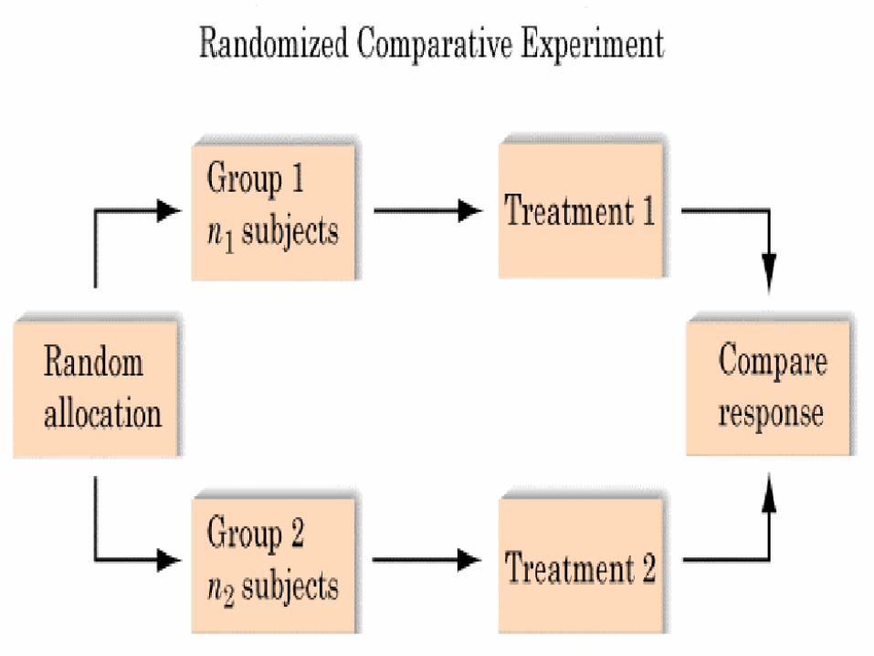
4. Experiments Researcher changesesearcher changes one thing (independent variable,

IV; called treatment in textbook); keeps everything else the same, and determines if behavior (dependent variable, DV) is affected.

5

Basic design is two groups where one group gets one level of the IV and the other gets another level of the IV (this includes its absence).

Since everything else kept constant, then any change in behavior (DV) is due to the change in the IV.

Can make cause and effect (what causes what) statements with experiments.

Cause and effect statements can only be made about groups; not individuals. They are probable causes not certain ones (remember: statistics is about probability not certainty).

6

7

Ex., Does a tutor impact academic performance?

Group A No tutor in RM

Group B A tutor in RM

Both groups are otherwise the same.

Compare grades in RM.

8

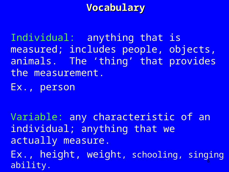
Vocabulary Vocabulary

Individual: anything that is measured; includes people, objects, animals. The ‘thing’ that provides the measurement.

Ex., person

Variable: any characteristic of an individual; anything that we actually measure.

Ex., height, weight, schooling, singing ability.

9

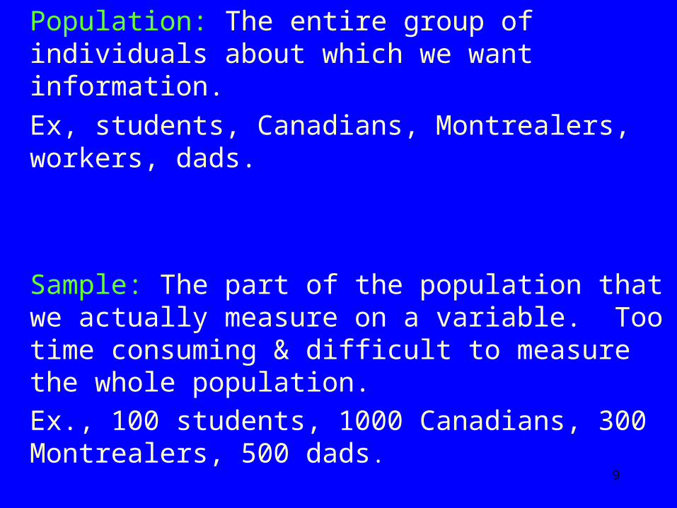
Population: The entire group of individuals about which we want information.

Ex, students, Canadians, Montrealers, workers, dads.

Sample: The part of the population that we actually measure on a variable. Too time consuming & difficult to measure the whole population.

Ex., 100 students, 1000 Canadians, 300 Montrealers, 500 dads.

10

Exercises Chapter 1

1. Fewer women than men vote for the PQ. A political scientist interviewed 400 male and female voters and asked how they voted in the last election.

a) Is this an experiment?

b) What is the population?

c) What is the sample?

d) What is the individual?

e) What is the variable under study?

11

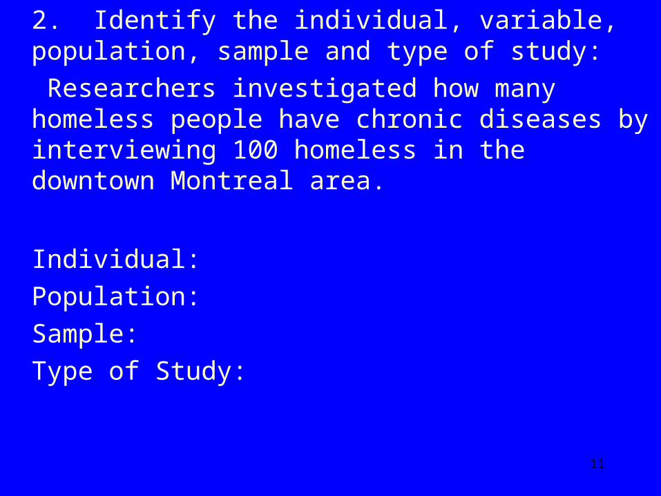
2. Identify the individual, variable, population, sample and type of study:

Researchers investigated how many homeless people have chronic diseases by interviewing 100 homeless in the downtown Montreal area.

Individual: Population: Sample: Type of Study:

12

3. As a researcher you are interested in whether students who sleep one hour more per night would improve their academic performance.

Design an experiment to investigate this. Be sure to identify the independent variable, the dependent variable, the population and the sample.

13

Chapter 4 - continuedChapter 4 - continued

Samples, Good and BadSamples, Good and Bad

Probability Sample

Any sample that is chosen by chance. Includes

Simple Random Sample (SRS) and Stratified Samples.

1. Simple Random Sample

Gives each individual in the population an equal chance of being chosen.

14

Use table of random digits (handout) or computer program to choose individuals or samples.

Random: every individual or sample has an equal chance of being picked.

This ensures the sample is representative of the population.

Therefore, we can generalize the results back to the population.

15

Choose a Simple Random Sample (SRS)

Step 1. Assign a number to every individual in the population (or to every sample).

Assign numbers beginning with 0 and keep going until everyone has a number. Go down columns of lists.

Step 2. Use random digits to select the numbers and choose those people.

16

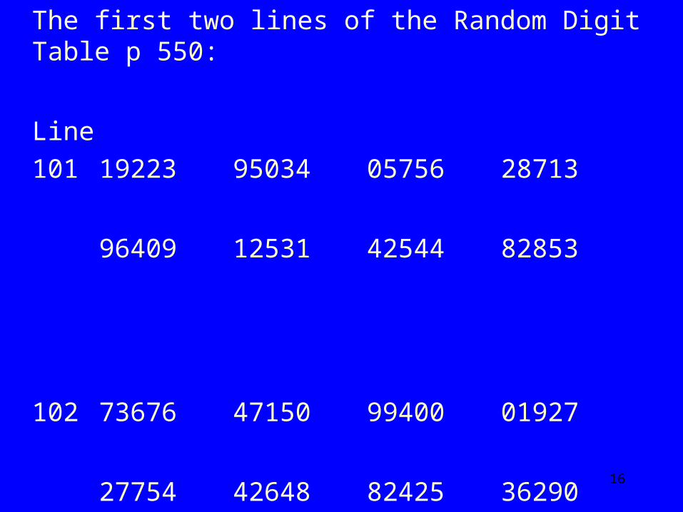
The first two lines of the Random Digit Table p 550:

Line 101 19223 95034 05756 28713

96409 12531 42544 82853

102 73676 47150 99400 01927

27754 42648 82425 36290

17

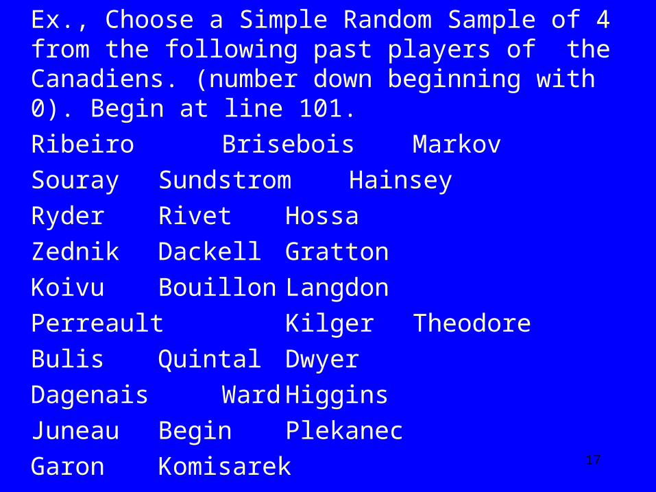
Ex., Choose a Simple Random Sample of 4 from the following past players of the Canadiens. (number down beginning with 0). Begin at line 101.

Ribeiro Brisebois Markov Souray Sundstrom Hainsey Ryder Rivet Hossa Zednik Dackell Gratton Koivu Bouillon Langdon Perreault Kilger Theodore Bulis Quintal Dwyer Dagenais Ward Higgins Juneau Begin Plekanec Garon Komisarek

18

The sample of 4 is: Komisarek (19); Hossa (22); Perreault (05); Dackell (13).

19

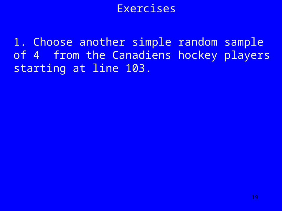
Exercises

1. Choose another simple random sample of 4 from the Canadiens hockey players starting at line 103.

20

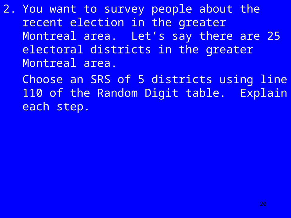
2. You want to survey people about the recent election in the greater Montreal area. Let’s say there are 25 electoral districts in the greater Montreal area.

Choose an SRS of 5 districts using line 110 of the Random Digit table. Explain each step.

21

Chapter 4Chapter 4

What Do Samples Tell UsWhat Do Samples Tell Us

22

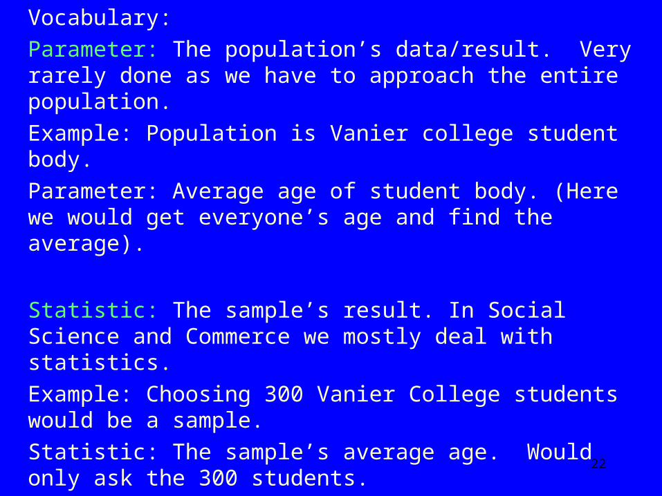
Vocabulary: Parameter: The population’s data/result. Very rarely

done as we have to approach the entire population. Example: Population is Vanier college student body. Parameter: Average age of student body. (Here we

would get everyone’s age and find the average).

Statistic: The sample’s result. In Social Science and Commerce we mostly deal with statistics.

Example: Choosing 300 Vanier College students would be a sample.

Statistic: The sample’s average age. Would only ask the 300 students.

23

Sampling Variability: When we take many samples from the same population, their results (statistics) vary slightly from one another.

The results do so in a pattern called the normal distribution unless they are not properly selected samples.

When the sample is large and well selected, the sample statistic is close to the the population parameter.

24

The larger the sample, the less the variabilityvariability up to sample size of about 1500.

Sample sizes beyond 1500 do not help to reduce the variability.

Variability: describes how spread out the values of the sample statistic are when taking many samples.

To reduce variability: Use larger samples.

25

Exercises for Chapter 4

1. A Crop/LaPresse poll found that 780 of 1000 elderly Montrealers were worried about falling into poverty due to fixed incomes and depressed stock market.

a) What is the sample?

b) What is the population?

c) Can we determine the statistic?

d) Can we determine the parameter?

26

2. A newspaper presents a survey where 500 of 1100 people coming out of the cinema said they went to see an action movie.

a) What is the sample?

b) What is the population? c) Can we determine a statistic?

d) Can we determine a parameter?

27

3. 1200 college students, evenly divided per gender, were asked about part-time work. 850 said they worked at least 12 hours per week.

a) What is the sample?

b) What is the population?

c) Can we determine a statistic?

d) Can we determine a parameter?

28

Chapter 4Chapter 4

How sample surveys go wrong: 1. Sampling errors:1. Sampling errors: errors that occur as we secure the

sample causing the sample to be different from the population. Biased samples.

a) convenience sampling:a) convenience sampling: grab them where you can. ex., Malls, stores.

b) voluntary/self -initiated response sample:b) voluntary/self -initiated response sample: interested people decide to participate given a public request.

ex., Call in votes; internet polls.

29

c) Undercoverage: when some groups in the population are left out of the process of choosing a sample.

Ex., homeless, people without phones or unlisted numbers.

d) Nonresponse - selected people who can’t be reached or decline to participate; this can be a serious problem as certain groups tend to decline more than others (ex., elderly, very busy women).

Nonresponse can exceed 70% of initial sample. Public opinion polls don’t give the percent of nonrespondents.

30

2. Random sampling errors:2. Random sampling errors: difference between the sample result (statistic) and the population result (parameter) caused by chance in selecting the random sample.

Ex., margin of error in a confidence statement

31

3. Nonsampling errors:3. Nonsampling errors: errors that occur after securing the sample.

a) Processing errors - mistakes when entering data. Easier now with computers.

b) Response error - person offers an incorrect response; makes a mistake.

c) Wording of questions - can influence the response. Ex., Should we maintain day care places at $5 per

day? Should the state subsidize day cares so they can

charge $5 per day?

32

When we want to ensure specific groups are When we want to ensure specific groups are represented: Use Stratified Random Sampling:represented: Use Stratified Random Sampling:

Proportional Stratified Random Sample 1. Divide the population into distinct groups according

to an important factor (ex., gender, age, residence location). Each group, or layer, called a stratum (strata is plural).

To have a proportional stratified random sampleproportional stratified random sample we choose the same percentage of each strata as is present in the population.

33

2. Take a separate SRS in each stratum and combine them to make the whole sample.

Ex., Social Science and Commerce Program Want to know opinion about computer facilities.

Know we should divide the groups into Social Science and Commerce because each group uses the computer facilities differently.

Want a sample of 200 students.

34

Step 1

Have 1000 Social Science and 250 Commerce students. These are the two strata.

To find proportion/percent in each group:

Total 1000 + 250 = 1250

Social Science = 1000/1250 = 80% or .8 proportion.

Commerce = 250/1250 = 20% or .2 proportion.

20% are Commerce students and 80% are Social Science students.

35

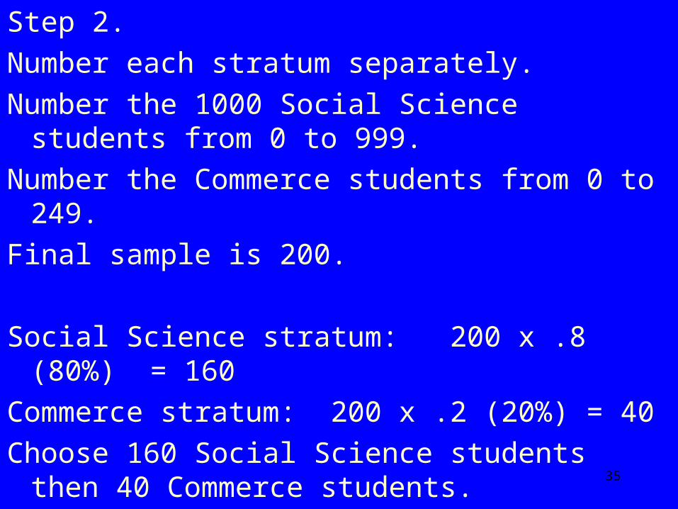
Step 2.

Number each stratum separately.

Number the 1000 Social Science students from 0 to 999.

Number the Commerce students from 0 to 249.

Final sample is 200.

Social Science stratum: 200 x .8 (80%) = 160

Commerce stratum: 200 x .2 (20%) = 40

Choose 160 Social Science students then 40 Commerce students.

36

3. Recent survey results show that 35% of college students graduate with over $1500 in debt. This is very different from the 65% usually reported. The survey used 1500 respondents after attempting to contact 4000.

a) What is the response rate for the survey?

37

CHAPTER 2CHAPTER 2 MEASURINGMEASURING

Measurement: assigning a number to represent a quality of a thing/person.

Ex, age, height, speed, depression, elation.

A measurement is valid when it measures an object/person in an appropriate manner.

It is a plausible and reasonable reflection of the meaning of the broader theory:

Ex., measure height in inches or centimeters; not in speed, time; Social status in terms of wealth or political rank. What about Conrad Black?

38

A measurement is reliable when the same answer is obtained over multiple measurements of the same variable. Ex., height.

What is a valid measurement for school performance?

What is a valid measurement for helping behavior?

39

A measurement can be in a count (frequency) or in a rate (proportion or percent).

Usually, a rate is better. Offers the advantage of comparing two different measurements.

Ex., Metro is 2 minutes late 10 times = count. Bus is 2 minutes late 25 times = count.

Metro is 2 minutes late 10% of the time = rate. Bus is 2 minutes late 15% of the time = rate.

40

Predictive Validity: A measurement has predictive validity if it can be used to predict success or performance on tasks that are related to what we measured.

Ex., Do college grades predict university grades? To some extent yes, but motivation and drive are

missing from the prediction. (ref: p. 141) SAT (Scholastic Aptitude Tests) and high school

grades predict about 34% of the variation in college grades. This means that about 1/3rd of the grade differences in college are predicted by the grades in high school and on the SAT tests.

41

Three types of errors in measurementThree types of errors in measurement.

1. Measuring something in an invalid manner.

2. A biased measurement - repeatedly overestimating or underestimating the value.

Ex., How many hours I will study next week.

3. Unreliable - the results of repeated measurements change from one time to the next.

If the differences in results are small can use an average to get a good approximation of the true score.

Ex., the clocks in the college.

42

Exercises Chapter 1

1. Give a valid way to measure determination.

2. Give an example of a biased measurement.

3. Give an example of a reliable measurement.

43

CHAPTER 4CHAPTER 4

1. Introduction to statistical inference.

2. What is a Confidence Interval.

3. What is a Test of Significance.

44

INTRODUCTION TO STATISTICAL INFERENCEINTRODUCTION TO STATISTICAL INFERENCE

Statistical inference is a technique to make decisions regarding the probability that the population would behave in the same way as the sample.

As it is based on probability, then the rules of probability must be followed. Therefore, the assumptions which must be met are:

1) Randomness: the predictable pattern of outcomes after very many trials.

1a) If samples are chosen randomly, then the pattern of outcomes is a normal distribution. This is called a sampling distribution.

45

2) We assume the mean of the normal distribution reflects the mean of the population parameter.

Statistical inference helps us determine how confident we are about where a result falls on the sampling distribution in two ways:

1. Confidence Intervals:1. Confidence Intervals: How confident we are that our sample’s result captured the population parameter within a certain range (margin of error).

2. Tests of significance: 2. Tests of significance: We make a claim about the population and use the sample’s results to test that claim. Want to determine the probability of our claim being right.

46

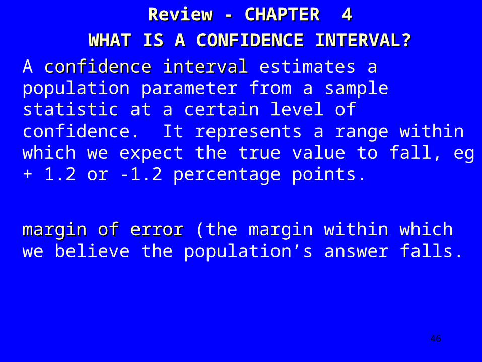
Review - CHAPTER 4Review - CHAPTER 4 WHAT IS A CONFIDENCE INTERVAL?WHAT IS A CONFIDENCE INTERVAL?

A confidence intervalconfidence interval estimates a population parameter from a sample statistic at a certain level of confidence. It represents a range within which we expect the true value to fall, eg + 1.2 or -1.2 percentage points.

margin of errormargin of error (the margin within which we believe the population’s answer falls. (Determined theoretically by taking many samples; Some of which fall above the true population mean and some fall below).

47

Here confidence means the probability of being right. We take the sample’s statistic (data) and estimate what the population’s answer would be. Involves how sure we are (confidence levelconfidence level) .

We take the samples’ statistic (data) and estimate what the population’s answer would be.

48

Involves how sure we are

(confidence level – a range within which we confidence level – a range within which we expect the true value to fallexpect the true value to fall), and

margin of error (or sampling error):margin of error (or sampling error): the difference between the true value of a characteristic in a population (eg; support for student fee hikes in college and university amongst ALL the students) and the value estimated from a random sample of the population.

49

error). of(margin scores of

margin certain awithin parameter

population thecapturingit of

level) (conf.y probabilit theestimate

and statisticany Take

samples from

(results) statisticsp̂

parameter population

p

50

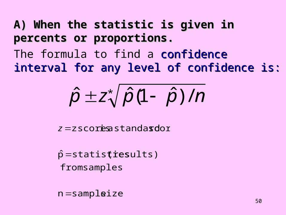
A) When the statistic is given in percents or A) When the statistic is given in percents or proportions.proportions.

The formula to find a confidence interval for any level confidence interval for any level of confidence is:of confidence is:

* /)ˆ1(ˆˆ nppzp

size sample n

samples from

(results) statisticsp̂

score standard a is score z

z

51

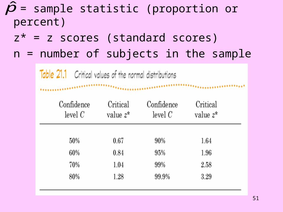
= sample statistic (proportion or percent) z* = z scores (standard scores) n = number of subjects in the sample

p̂

52

Example:

Mayor Villeneuve is two weeks from election day. He wants to know his chances of winning the election. A polling company asks 1000 people who they would vote for if the election were held today and 57% say Villeneuve.

Villeneuve wants to be 90% confident that he will win.

.57 + - .0256 or 57% plus and minus 2.5%

1000/)57.1(57.64.157.

53

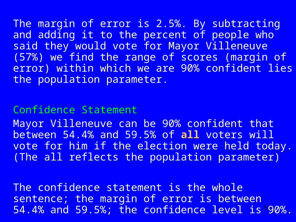
The margin of error is 2.5%. By subtracting and adding it to the percent of people who said they would vote for Mayor Villeneuve (57%) we find the range of scores (margin of error) within which we are 90% confident lies the population parameter.

Confidence Statement Mayor Villeneuve can be 90% confident that between

54.4% and 59.5% of all voters will vote for him if the election were held today. (The all reflects the population parameter)

The confidence statement is the whole sentence; the margin of error is between 54.4% and 59.5%; the confidence level is 90%.

54

Exercises 1. A sample of 500 students in Montreal was asked if

they graduated from college in debt and 58% of them said yes. Give a 99% confidence interval of all Montreal students who are in debt.

55

56

2. A sample of 1000 students in Montreal was asked if they graduated from college in debt and 58% of them said yes. Give a 99% confidence interval of all Montreal students who are in debt.

Using the same formula:

57

58

3. A sample of 1000 students in Montreal was asked if they graduated from college in debt and 58% of them said yes. Give a 90% confidence interval of all Montreal students who are in debt.

59

4. How does the sample size affect the margin of error?

5. How does the confidence level influence the margin of error?

60

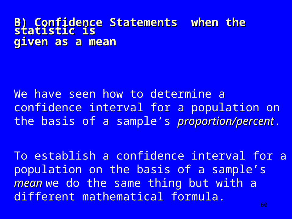
B) Confidence Statements when the statistic is B) Confidence Statements when the statistic is given as a meangiven as a mean

We have seen how to determine a confidence interval for a population on the basis of a sample’s proportion/percentproportion/percent.

To establish a confidence interval for a population on the basis of a sample’s mean mean we do the same thing but with a different mathematical formula.

61

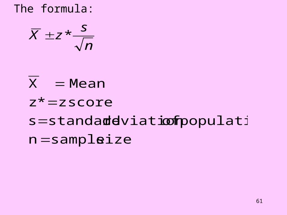
The formula:

size sample n

population ofdeviation standard s

score z *z

Mean X

*

n

szX

62

Example: The average debt of 500 students is $750 with a

standard deviation of $50. Make a confidence statement about the debt level of

all students at the 99% confidence level.

Using the formula:

500

5058.2750

63

750 +/- 2.58 (2.24)

750 +/- 5.77 Confidence statement: We are 99% confident that all

students are between $744.23 and $755.77 in debt.

64

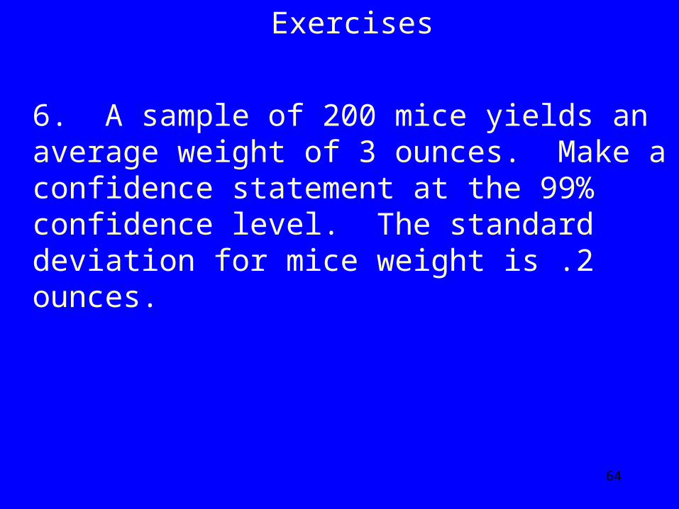
Exercises

6. A sample of 200 mice yields an average weight of 3 ounces. Make a confidence statement at the 99% confidence level. The standard deviation for mice weight is .2 ounces.

65

7. Using the mice data in question #1, make a confidence statement at the 85% confidence level.

66

8. Compare the margin of error for questions 1 & 2. Explain why they are different.

67

CHAPTER 22CHAPTER 22 What is a Test of Significance?What is a Test of Significance?

Statistical tests determine if the sample statistic (result) gives good evidence against a claim of no effect or no difference. This claim is the null hypothesis.

There are two types of hypotheses. 1. Null hypothesis (Ho): There is no difference or no

effect of what we are studying. The statistical test assesses the strength of the

evidence against the null hypothesis. This is the claim we seek evidence against.

68

2. Alternative (Experimental) Hypotheses (Ha) The alternative hypothesis states there is an effect or

a difference.

2a) One-tailed alternative hypothesis: States that the data states the direction of the

difference; the population’s answer (parameter) is either bigger or smaller than the null hypothesis.

69

2b) Two-tailed alternative hypothesis states there will be a difference between the sample’s data (statistic) and the null hypothesis but we don’t know if is larger or smaller.

70

71

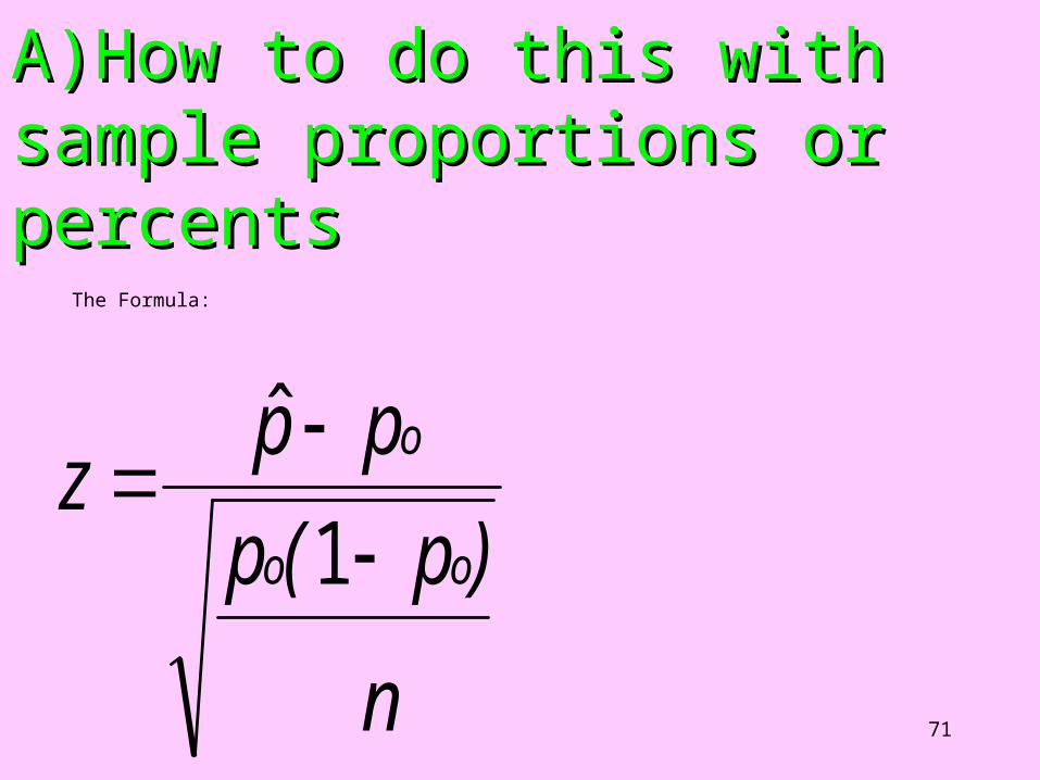
A)How to do this with sample A)How to do this with sample proportions or percentsproportions or percents

The Formula:

n

)p(p

ppz

oo

o

1

ˆ

72

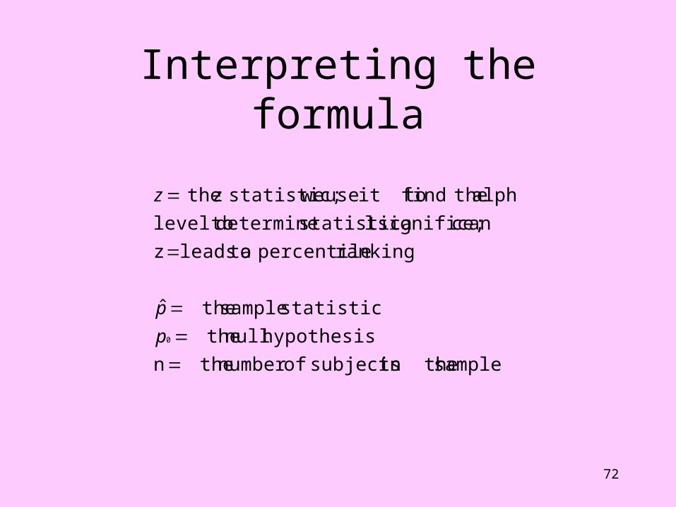
Interpreting the formula

sample in the subjects ofnumber then

hypothesis null the

statistic sample the ˆ

ranking percentile a toleads z

ce;significan lstatistica determine tolevel

alpha thefind it to use westatistic; z the

0

p

p

z

73

Ex. Perform a study on coffee preference: fresh or instant.

The null hypothesis would be that half the population would prefer fresh and half would prefer instant.

The alternative hypothesis is that more people prefer fresh coffee.

Result of study: 72% said they preferred fresh coffee. Sample size is 50.

74

ALWAYS TEST THE NULL HYPOTHESIS!!!

Null Hypothesis: Ho p = .5 (claims that 50% of the population would

prefer fresh; 50% would prefer instant.) The statistical test attempts to determine how much

evidence (sample statistic) exists against that claim.

How much evidence is needed to reject the null hypothesis claim is called the alpha level or significance level.

The alpha level is usually set at .05

75

The alpha level is usually set at .05 This means that the P-value (result of statistical test of significance) must be in the last 5% of the normal curve.

We are determining whether the result obtained from the research is sufficiently different from the large assumed population parameter so as to invalidates the null hypothesis.

NB: The null hypothesis always assumes no effect or no difference between preferences, opinions, groups.

76

Steps to Determining Statistical Significance.Steps to Determining Statistical Significance. Step 1: Develop a null hypothesis that states no effect

or no difference. Ex., no coffee preference. Ho = .5 (50% fresh; 50% instant) This is the assumed population parameter.

Step 2: Develop an alternative hypothesis that makes sense given the results from the sample. Ex., People prefer fresh coffee. p > .5 More than 50% of people.

NB: We hypothesize larger or smaller than the null hypothesis without putting a specific number.

77

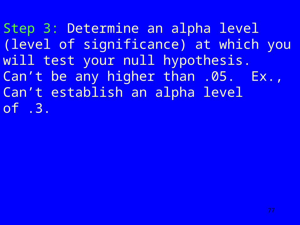
Step 3: Determine an alpha level (level of significance) at which you will test your null hypothesis. Can’t be any higher than .05. Ex., Can’t establish an alpha level of .3.

78

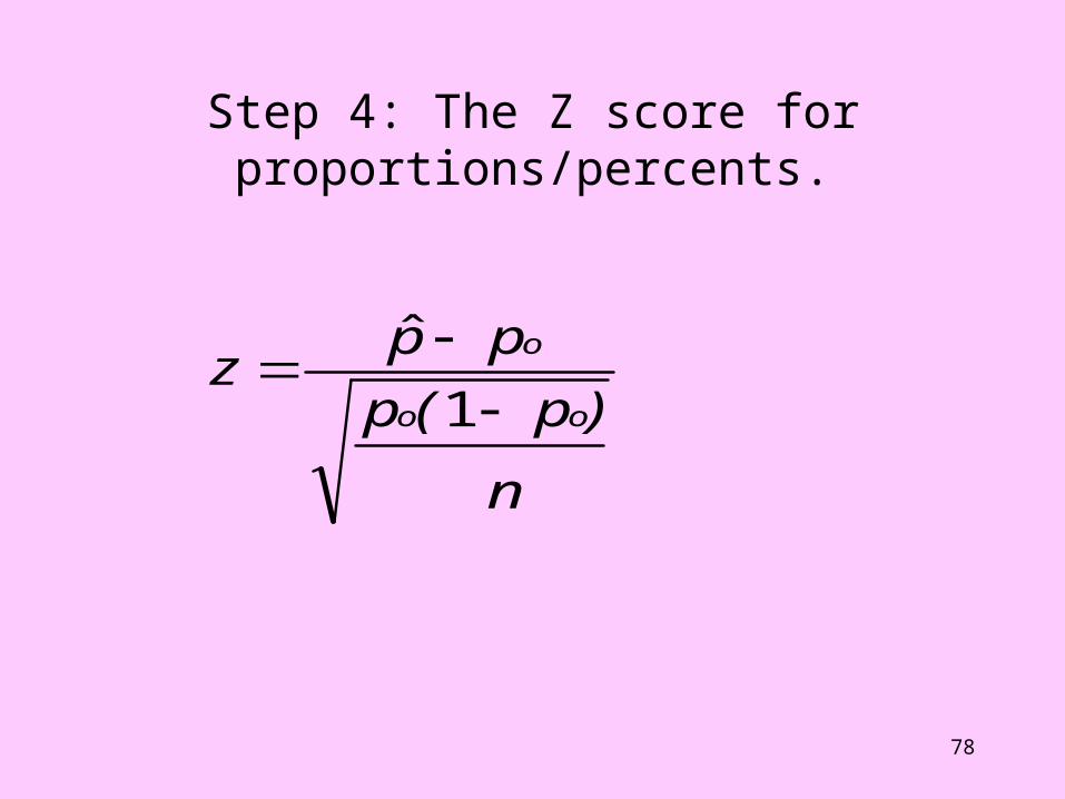
Step 4: The Z score for proportions/percents.

n

)p(p

ppz

oo

o

1

ˆ

79

The Z score cont.

50

)5.1(5.

572. .

z

80

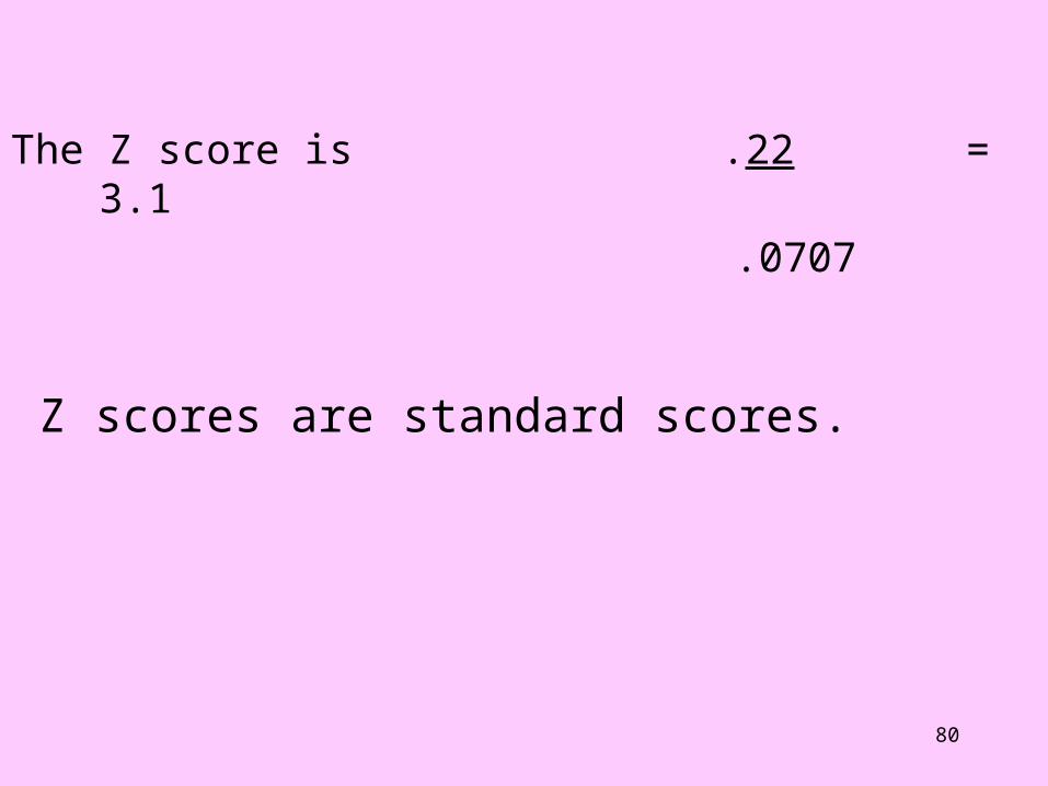
The Z score is .22 = 3.1 .0707

Z scores are standard scores.

81

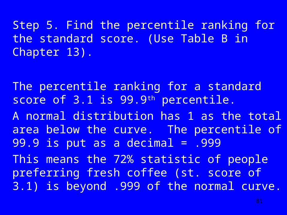
Step 5. Find the percentile ranking for the standard score. (Use Table B in Chapter 13).

The percentile ranking for a standard score of 3.1 is 99.9th percentile.

A normal distribution has 1 as the total area below the curve. The percentile of 99.9 is put as a decimal = .999

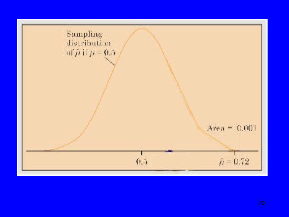
This means the 72% statistic of people preferring fresh coffee (st. score of 3.1) is beyond .999 of the normal curve.

82

That leaves .001 or .1% of the total area that is further than a st. score of 3.1

The .001 is called the P-valueThe .001 is called the P-value (result of statistical test).

Step 6

To reject the null hypothesis that there is no difference between the number of people in the population who prefer fresh and instant coffee we need to have a P-value smaller than .05 of the curve beyond the statistic.

83

As .001 is much smaller .05 (the level of significance), then we reject the null hypothesis that there is no difference between the number of people who like fresh and instant. Expressed as p<.05.

We then support the alternative hypothesis that there are a greater number of people in the population who prefer fresh coffee.

84

We have taken a sample statistic (72%) and compared it to the estimated population parameter (50%) for the null hypothesis and found that it permits us to reject that claim of no difference between number of people in the population who prefer fresh and who prefer instant.

But we are only 95% confident (.05 significance level) that we are right; there is no certainty.

85

• Exercises

• 1. It is known that 75% of all apple crops are profitable. This year a sample of 200 orchards showed that 76% of the crops were profitable.

• 1a) Develop a null hypothesis.

• 1b) Develop an appropriate alternative hypothesis.

86

• 1c) Is there a statistically significant greater percentage profit this year than previous years. Use the .05 significance level.

87

88

• Exercises• 1d) Would there have been a statistically • significant difference had you used the .01

significance level.

89

2. When asking a sample of 250 people if they believe increasing the size of the gas filter would results in greater gas mileage; 55% said yes.

2a) Develop a null hypothesis.

2b) Develop an appropriate alternative hypothesis.

90

2c) Using the .05 significance level, determine if we can reject the null hypothesis.

91

92

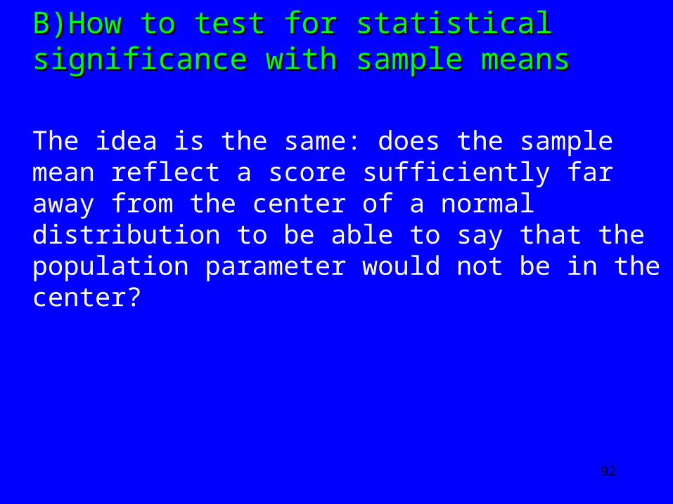
B)How to test for statistical significance with B)How to test for statistical significance with sample meanssample means

The idea is the same: does the sample mean reflect a score sufficiently far away from the center of a normal distribution to be able to say that the population parameter would not be in the center?

93

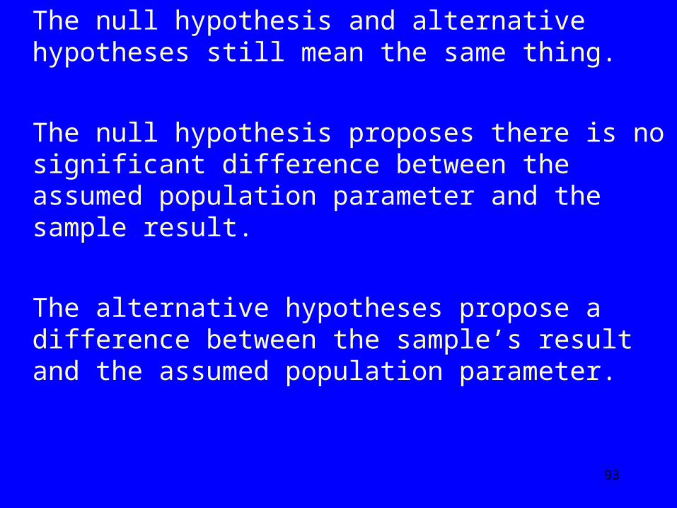
The null hypothesis and alternative hypotheses still mean the same thing.

The null hypothesis proposes there is no significant difference between the assumed population parameter and the sample result.

The alternative hypotheses propose a difference between the sample’s result and the assumed population parameter.

94

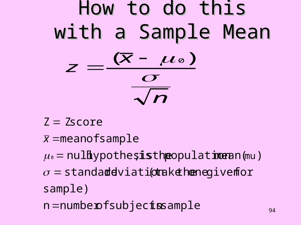
How to do thisHow to do thiswith a Sample Meanwith a Sample Mean

n

xz

)( 0

samplein subjects ofnumber n

sample)

forgiven one the(takedeviation standard

)(mean population theis ;hypothesis null

sample ofmean

score Z Z

mu0

x

95

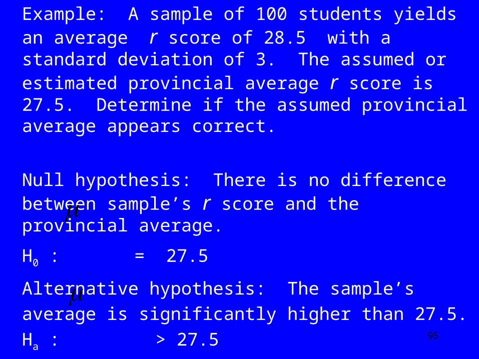
Example: A sample of 100 students yields an average r score of 28.5 with a standard deviation of 3. The assumed or estimated provincial average r score is 27.5. Determine if the assumed provincial average appears correct.

Null hypothesis: There is no difference between sample’s r score and the provincial average.

H0 : = 27.5

Alternative hypothesis: The sample’s average is

significantly higher than 27.5.

Ha : > 27.5

96

We will set the alpha level (level of significance) at .05.

Steps to calculating the P-value for a sample mean.

Step 1: Finding the Z score

n

xz

)( 0

97

score Z theis 33.3

3.1

100

3)5.275.28(

z

98

Step 2: Finding the P-Value:

Z Score (is a standard score) = 3.33 To translate a St. Score to a P-value we go to Table B

(p. 547) St. Score = 3.33 becomes a percentile of 99.95. Put the percentile in decimal form before subtracting

from 1.

99.95 = .9995 in decimal form.

The P-Value is 1 - .9995 = .0005 (Reminder: the complete area under a normal

distribution is equal to 1)

99

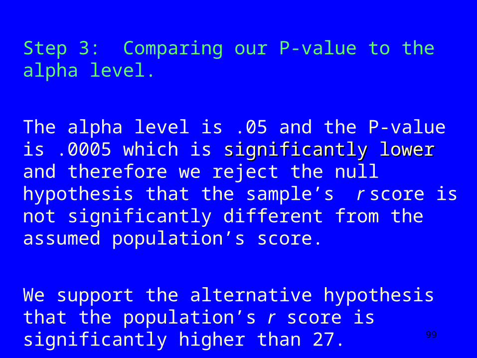
Step 3: Comparing our P-value to the alpha level.

The alpha level is .05 and the P-value is .0005 which is significantly lowersignificantly lower and therefore we reject the null hypothesis that the sample’s r score is not significantly different from the assumed population’s score.

We support the alternative hypothesis that the population’s r score is significantly higher than 27.

100

Exercises1. The average bike ride is 11 kilometers. A

sample of 100 adults rode an average of 12 kilometers per bike ride with a standard deviation of 2 kilometers.

Using the .05 level of significance, determine if the sample’s average bike ride is statistically significantly different from the population’s average.

101

2. A researcher finds that an increase in the size of the gas filter results in a mean of 32 miles per gallon with a standard deviation of 3. The sample size was 14. It is known that car model gets 30 miles per gallon with a regular size filter.

2a) Develop a null hypothesis.

2b) Develop an appropriate alternative hypothesis.

102

2c. Determine if there is a statistically significant difference between the gas filters. Use the .05 significance (alpha) level.

103

104

CHAPTER 14CHAPTER 14 DESCRIBING RELATIONSHIPS:DESCRIBING RELATIONSHIPS:

SCATTERPLOTS AND CORRELATIONSSCATTERPLOTS AND CORRELATIONS

Scatterplots:Scatterplots: Involves the relationship between two or more

quantitative (ordinal, interval, ratio) variables measured on the same individuals/objects.

(For our course, we will deal with two variables.)

105

The graph that depicts this relationship is called a scatterplot.scatterplot.

Sometimes, scatterplots have an explanatory variable (on the horizontal axis) and a response variable (on the vertical axis).

The explanatory variable is the independent variable. The response variable is the dependent variable.

106

Each dot in a scatterplot reflects two pieces of information (variables) about an individual.

In this example, the individuals are countries. The graph depicts the relationship between gross domestic product per person and longevity. (p. 271)

107

Some scatterplots have no explanatory and response variables; only the relationship between two variables.

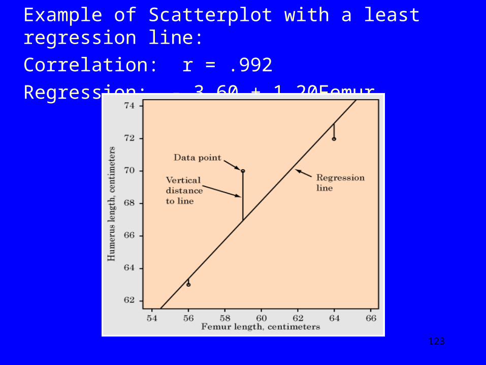
Ex., The Archaeopteryx: the femur (leg bone) and humerus (arm bone); the size of one does not ‘explain’ or ‘contribute’ to the size of the other. (p. 274)

108

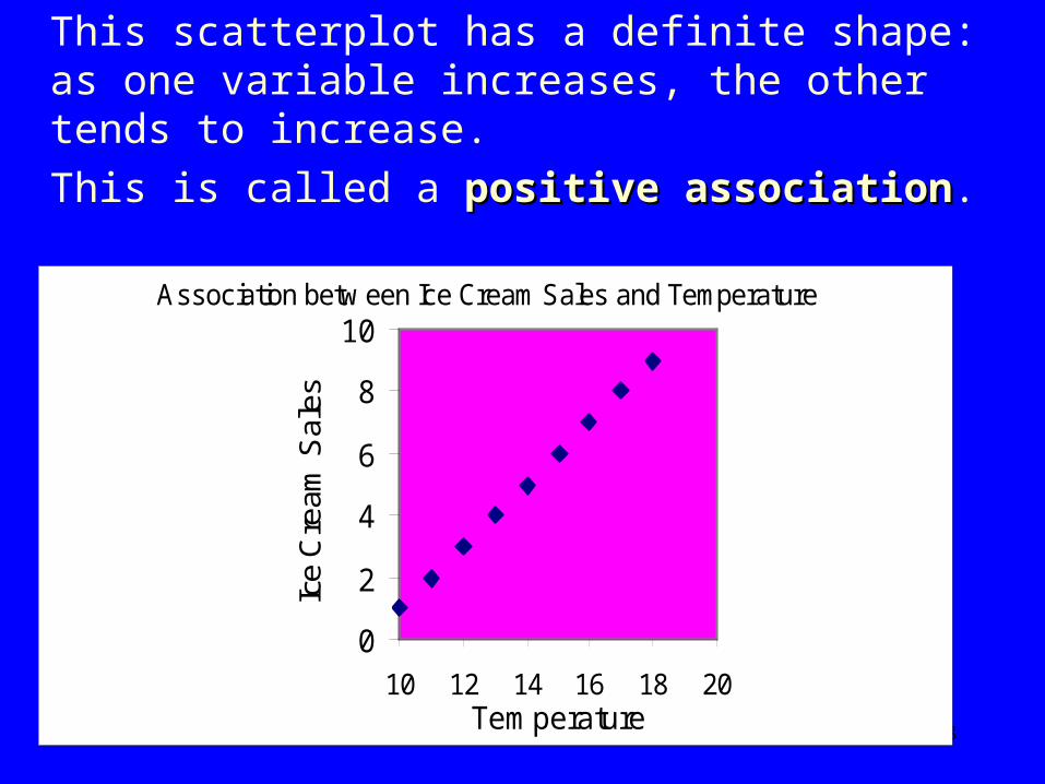
This scatterplot has a definite shape: as one variable increases, the other tends to increase.

This is called a positive associationpositive association.

Association betw een Ice Cream Sales and Temperature

0

2

4

6

8

10

10 12 14 16 18 20Temperature

Ice

Cre

am S

ales

109

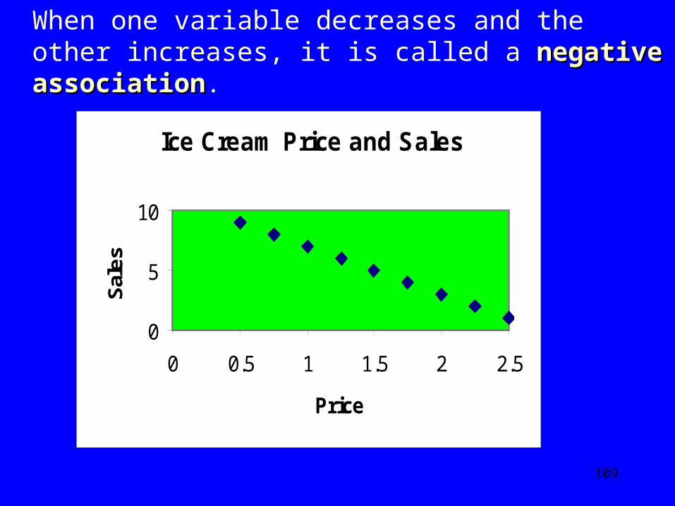
When one variable decreases and the other increases, it is called a negative associationnegative association.

Ice Cream Price and Sales

0

5

10

0 0.5 1 1.5 2 2.5

Price

Sal

es

110

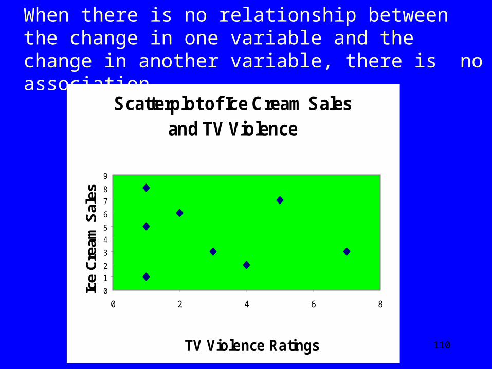
When there is no relationship between the change in one variable and the change in another variable, there is no association.

Scatterplot of Ice Cream Sales and TV Violence

0

12

3

45

6

78

9

0 2 4 6 8

TV Violence Ratings

Ice

Cre

am S

ales

111

To examine a scatterplot:

1. Look at the overall pattern and any important deviations.

2. Describe the scatterplot using the form, direction and strength of the relationship.

3. Look for outliers

4. The closer the data are to forming a linear line, the stronger the association.

Ex., The Archaeopteryx: There is a strong positive association between the size of the femur and the humerus with no outliers.

112

When the association between two variables is expressed mathematically, it is called a correlation.correlation.

Features of Correlations 1. It is expressed as r.

2. The range is from -1.00 to +1.00.

3. -1.00 is a perfect negative correlation; +1.00 is a perfect positive correlation. These are never seen with real data. Zero is no correlation - there is no relationship between the variables.

113

4. Correlations use standard scores so we can compute them for any two variables (doesn’t have to be the same unit of measurement).

5. Correlations measures the strength of straight-line (linear) associations between variables.

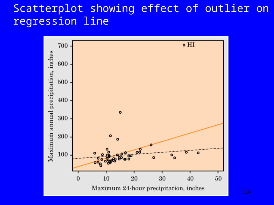
6. Correlations are affected by outliers. The more data there is, the less an outlier will influence the correlation.

114

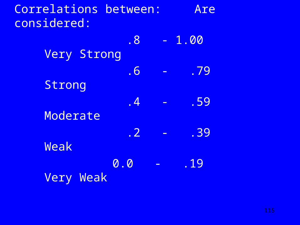
115

Correlations between: Are considered: .8 - 1.00 Very Strong .6 - .79 Strong .4 - .59 Moderate .2 - .39 Weak 0.0 - .19 Very Weak

116

Exercises

1. Develop a scatterplot for the following data: Running times for 100 meter dash.

Trial 1 10 11 10.5 10.2 10

Trial 2 9.9 10.9 10.6 10.2 9.8

117

118

2. What is wrong with the following statements: a) The correlation between number of hours worked

by students and number of times they answer a question in class is r = .5

b) The correlation between the first snow storm of any given year and the number of car accidents that day is r = - 1.3

119

c) The correlation between gender and income is about r = .66

3. Give an example for each of the following: a) A strong positive correlation

b) A strong negative correlation

c) No correlation

120

CHAPTER 15CHAPTER 15

DESCRIBING RELATIONSHIPS:DESCRIBING RELATIONSHIPS:

REGRESSION, PREDICTION AND REGRESSION, PREDICTION AND CAUSATIONCAUSATION

Regression and PredictionRegression and Prediction

Uses two or more ordinal, interval or ratio variables.

Formula used to predict the value of one variable by using the value of a second variable.

121

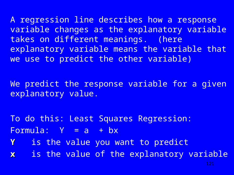
A regression line describes how a response variable changes as the explanatory variable takes on different meanings. (here explanatory variable means the variable that we use to predict the other variable)

We predict the response variable for a given explanatory value.

To do this: Least Squares Regression: Formula: Y = a + bx Y Y is the value you want to predict x x is the value of the explanatory variable

122

aa is the intercept - the value of the response variable (y) when the explanatory value (x) is 0. It is where the least square regression line cuts across the x axis.

bb is the slope of the least square regression line. The amount by which the response variable (y)

changes when the explanatory variable (x) increases by one unit (of whatever is being measured).

Minitab calculates the slope and intercept for us; we plug data into the formula.

Can place a least square regression line on a scatterplot by putting a line through the data points.

123

Example of Scatterplot with a least regression line: Correlation: r = .992 Regression: - 3.60 + 1.20Femur

124

Scatterplot showing effect of outlier on regression line

125

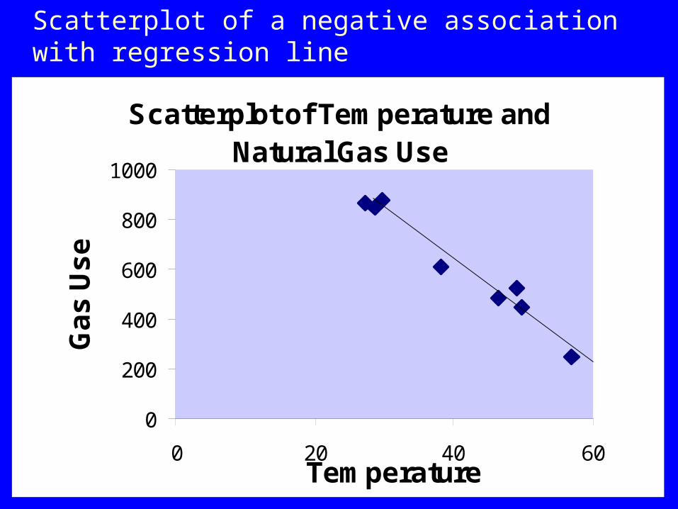
Scatterplot of a negative association with regression line

Scatterplot of Temperature and Natural Gas Use

0

200

400

600

800

1000

0 20 40 60Temperature

Ga

s U

se

126

We cannot predict response values for explanatory values that are out of the range of the data.

Ex., gas and temperature. We should not predict beyond the given temperatures.

As prediction involves only associations between variables, they do not address cause and effect; therefore, no statements about causality.

127

Coefficient of determination (rCoefficient of determination (r22) :) : The square of the correlation (r2) gives the total

amount of change in one variable that is due to changes in the other variable.

Does not mean one variable causes the other; only that some of the change in the first is due to change in the second.

Ex., r = .5 between temperature and level of outdoor activity.

r2 = .25 which means that 25% of the change (variation) in the outdoor activity variable is linked to change in the temperature variable.

128

EXERCISES 1. Professor Lively, runs every day for at least 30

minutes and checks her pulse rate. Some of the data, from p. 276: Time PulseTime Pulse 34.12 152 35.52 124 34.52 140 34.05 152 34.13 146 35.52 128 36.17 136

129

1a) Draw a scatterplot for these data.

130

1b) The correlation, r = -.815 Briefly describe what this means.

1c) Draw a least square regression line in the scatterplot (eyeball method).

131

1d) The least square regression formula is: 510 - 10.6 time Predict the pulse rate for 34.5 minutes eyeballing the

scatterplot.

Then predict the pulse rate using the formula.

Compare the results.

132

2. The following are the closing quotes for the Nasdaq and Microsoft for ten trading days.

Nasdaq: Microsoft:• 1742 54• 1785 57• 1770 55• 1789 56• 1784 56• 1804 57• 1862 60• 1845 60• 1826 59• 1824 59

133

The scatterplot with regression line for these data.

134

2a) The correlation is r = .974 Describe what this means.

135

• 4. The correlation between hours of sunshine and number of strawberries on a plant is r = .67. What percentage of strawberry production is linked to hours of sunshine?

136

Causation: The reason something occurs; what makes it happen. Requires experimental research designs where there

is a great deal of control of all variables.

Philosophically, causation requires a ‘leap of faith’ from excluding all other possible explanations to granting the independent variable the power to have caused the behavior.

137

a) Simple Causation: Very rare in real life. A causes B to happen. Ex., paying students $250 to get 80%+ in a course.

This would increase the number of students who get 80%+.

If everything else is kept constant, we could say that the $250 had an effect on students’ behavior; it caused caused an increase in grades.

A B

138

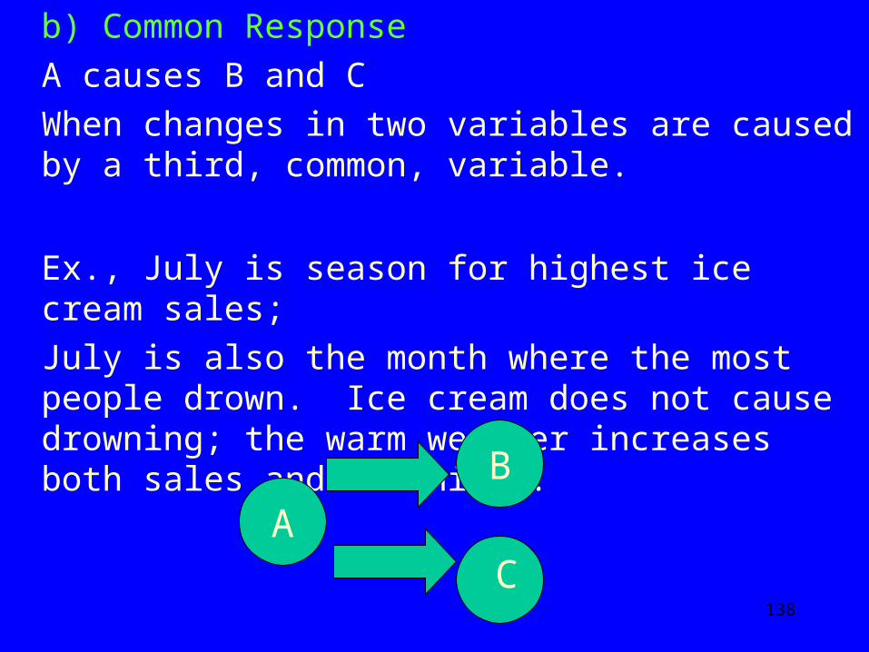
b) Common Response A causes B and C When changes in two variables are caused by a third,

common, variable.

Ex., July is season for highest ice cream sales; July is also the month where the most people drown.

Ice cream does not cause drowning; the warm weather increases both sales and drownings.

A

B

C

139

c) Confounding Response: We know two variables cause a change in a third but

we don’t know the ‘weight’ of each variable.

Ex., person smokes and drinks too much. Heart is affected; we know that both contribute but do

not know how much each contribute. Need to do experimental research to ‘sort out’ the

influences.

Helps to isolate each variable’s effect on heart.

140

When experimentation is not possible, we can approach causation if the following conditions are met:

1. The association between two variables is strong.

2. The association between two variables is consistent.

3. The alleged cause precedes the effect.

4. The alleged cause is plausible.

141

3. People who drink diet soft drinks tend to gain more weight over a one year period than people who do not.

Does drinking diet drinks make people gain weight? Give a more plausible explanation.

142

Chapter 24Chapter 24 Two-Way Tables and the Chi-Square TestTwo-Way Tables and the Chi-Square Test

Two- Way Tables:Two- Way Tables: Displays results as percents or frequency for two variables.

Use for nominal (categorical) variables or with one nominal variable and one ordinal or interval variable.

Good for surveys.

143

Example Distribution of Employed in a Very Small Town

Ages 15-24 25-34 35-44 45+

F 20 25 50 50

M 30 35 60 75

These data are put in bar graphs.

First thing to do is to sum all rows, columns and grand total.

144

Types of questions asked of two-way tables: A) What percent of the sample is male? Total sample = 345 Total male = 200 Percent male = 58%

B) What percent of the sample is between 15-24 years old?

Total sample = 345 Total 15-24= 50 Percent 15-24 = 14.5%

145

C) What percent of the sample are males between 35-44 years old?

Total sample = 345 Males 35-44 = 60 % males 35-44 = 17.4%

D) What percent of females are 25-34 years old? Total females = 145 Females 25-34 = 25 % females 25-34 = 17.2%

146

The other way to explore data in a two-way table is to investigate whether there is an association between the two variables that would also be reflected in the population. To do this use a test of significance.

(Hint: whenever we want to generalize to the population we have to use a confidence interval or a test of significance).

The test of significance is called the Chi-Square Test. It is very often used when analyzing surveys.

147

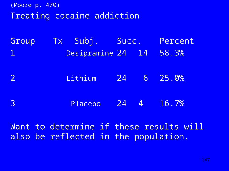
(Moore p. 470)

Treating cocaine addiction

Group Tx Subj. Succ. Percent 1 Desipramine 24 14 58.3%

2 Lithium 24 6 25.0%

3 Placebo 24 4 16.7%

Want to determine if these results will also be reflected in the population.

148

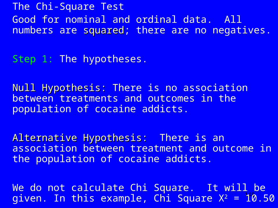
The Chi-Square Test Good for nominal and ordinal data. All numbers are

squaredsquared; there are no negatives.

Step 1: The hypotheses.

Null Hypothesis:Null Hypothesis: There is no association between treatments and outcomes in the population of cocaine addicts.

Alternative Hypothesis:Alternative Hypothesis: There is an association between treatment and outcome in the population of cocaine addicts.

We do not calculate Chi Square. It will be given. In this example, Chi Square X2 = 10.50

149

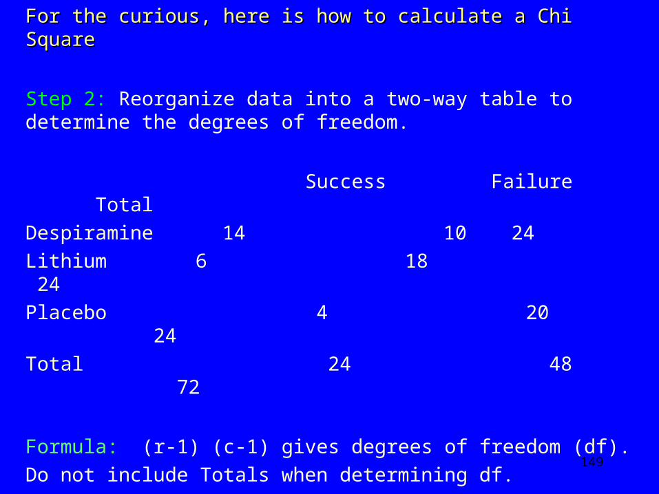
For the curious, here is how to calculate a Chi SquareFor the curious, here is how to calculate a Chi Square

Step 2: Reorganize data into a two-way table to determine the degrees of freedom.

Success Failure Total Despiramine 14 10 24 Lithium 6 18 24 Placebo 4 20 24 Total 24 48 72

Formula: (r-1) (c-1) gives degrees of freedom (df). Do not include Totals when determining df.

150

Degrees of freedom is a statistical concept that identifies how many categories must be known for all of them to be known.

Ex. If something is in either a red box or a blue box and you know it can’t be in the red box then by elimination it must be in the blue box. Here the df is 1; only one thing must be fixed for you to know the other thing.

We must know how to use Degrees of Freedom The df for Chi Square involves both rows and

columns. Formula: (r-1) (c-1) gives degrees of freedom (df).

151

We ‘place’ our chi-square result on the distribution to see if to falls far enough to reject the null hypothesis of no difference between treatment and outcomes.

The distribution for the chi-square is not a normal distribution; it is a curve that is skewed to the right.

As the formula uses squares, then there can be no negative values.

This curve changes depending upon the degrees of freedom.

152

The curves below depict the chi-square distribution for differing degrees of freedom.

We can see that as the df increases, the curve becomes less skewed to the right and we get larger values.

153

For our cocaine example, the degrees of freedom are: (3-1) (2-1) = 2 df

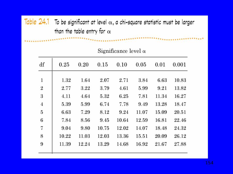
We use a table to determine if we attain statistical significance.

154

155

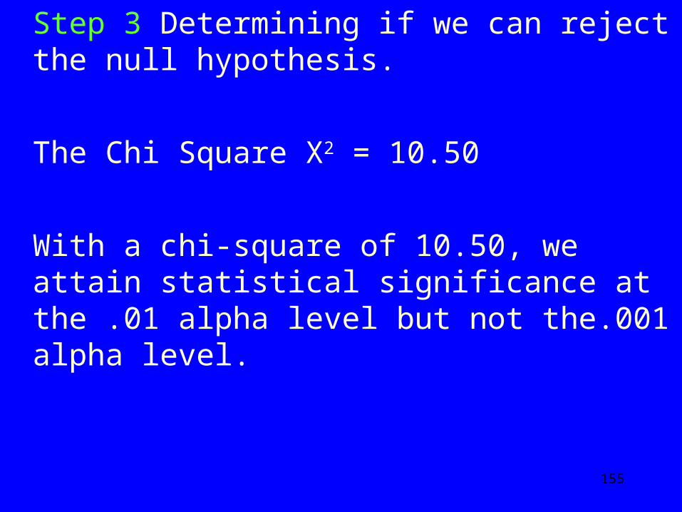
Step 3 Determining if we can reject the null hypothesis.

The Chi Square X2 = 10.50

With a chi-square of 10.50, we attain statistical significance at the .01 alpha level but not the.001 alpha level.

156

Therefore, we can say that there are statistically significant relationship between treatments and outcomes for the population beyond the .01 alpha level (p > .01).

When we observe statistical significance, we then go back to the table to determine where it lies.

In the cocaine example, it is obvious that desipramine treatment fares better than the others.

157

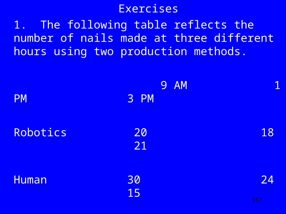
Exercises 1. The following table reflects the number of nails

made at three different hours using two production methods.

9 AM 1 PM 3 PM

Robotics 20 18 21

Human 30 24 15

158

1a) What percent of nails are produced at 1 PM?

1b) What percent of nails are produced with robotics?

159

1c) What percent of the nails produced at 3 PM are human made?

1d) What percent of the robotic made nails are produced at 9 AM?

160

2. A researcher investigates whether there is any association between time of production and method of production.

2a) Give a null hypothesis.

2b) Give an alternative hypothesis.

161

2c) The chi-square statistic is X2 = 6.04 Is this statistically significant at or beyond the .05 alpha level?

162

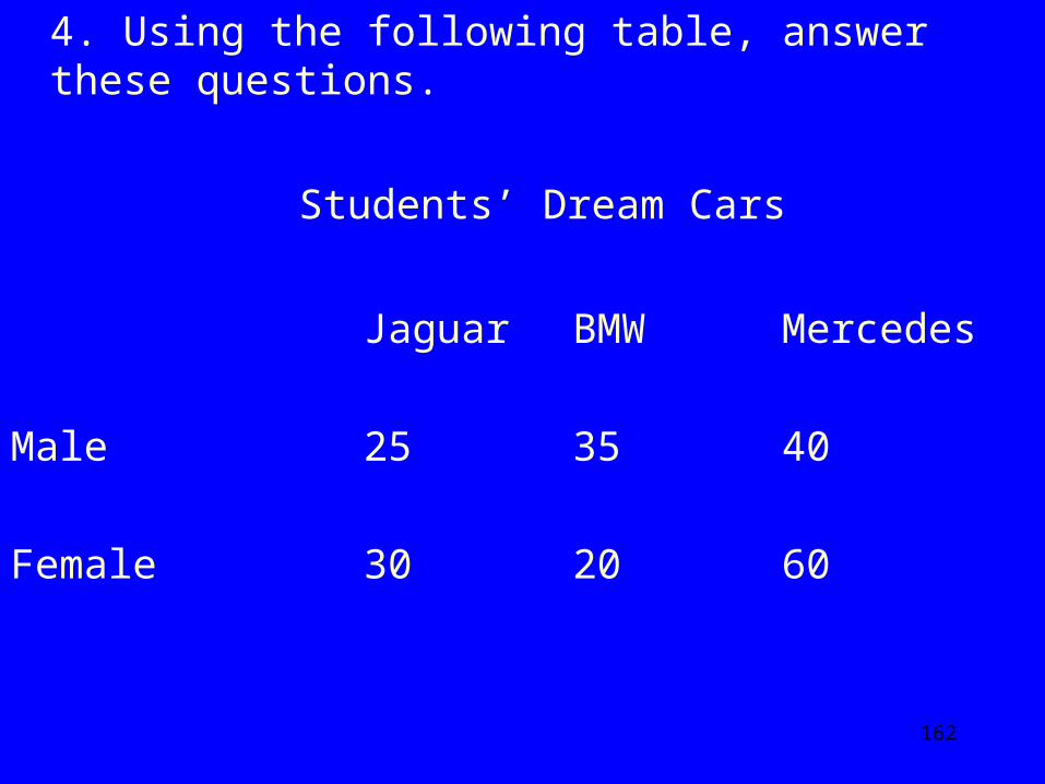
4. Using the following table, answer these questions.

Students’ Dream Cars

Jaguar BMW Mercedes

Male 25 35 40

Female 30 20 60

163

4a) What percent of women want a Jaguar?

4b) What percent of the sample want a BMW?

164

4c) What percent of people who want Mercedes are men?

165

4d) The Chi Square X2 is 8.088 for the relationship between gender and car preference. Determine whether this is statistically significant beyond the .05 alpha level.

4e) Describe the association.

166

CHAPTER 16CHAPTER 16

CONSUMER PRICE INDEXCONSUMER PRICE INDEX

Index number: Describes the percent change from a base (comparison) period.

Use index points to be able to compare ‘apples and oranges’.

Anything can be put into an index number. Most frequently, it is the cost of a service/good.

Formula for index number: value x 100 base value

Index number for base value is always 100.

167

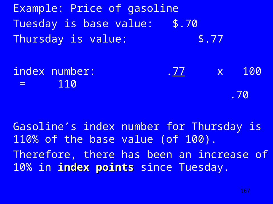
Example: Price of gasoline Tuesday is base value: $.70 Thursday is value: $.77

index number: .77 x 100 = 110 .70

Gasoline’s index number for Thursday is 110% of the base value (of 100).

Therefore, there has been an increase of 10% in index pointsindex points since Tuesday.

168

Usually, an index number does not reflect the price change of one item; most often it reflects the change in a ‘basket of services/goods’ over a period of time.

These baskets are fixedfixed; once you determine the items and quantities in the basket for the base year they cannot change for the comparison years.

169

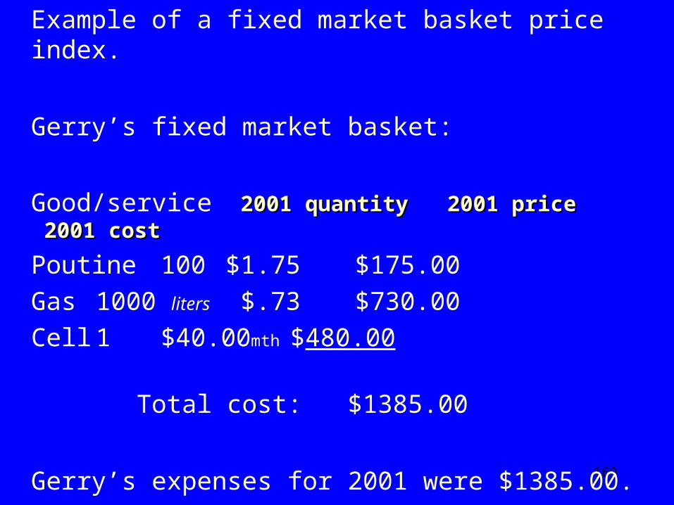
Example of a fixed market basket price index.

Gerry’s fixed market basket:

Good/service 2001 quantity 2001 price 2001 2001 quantity 2001 price 2001 costcost

Poutine 100 $1.75 $175.00 Gas 1000 liters $.73 $730.00 Cell 1 $40.00mth $480.00 Total cost: $1385.00

Gerry’s expenses for 2001 were $1385.00.

170

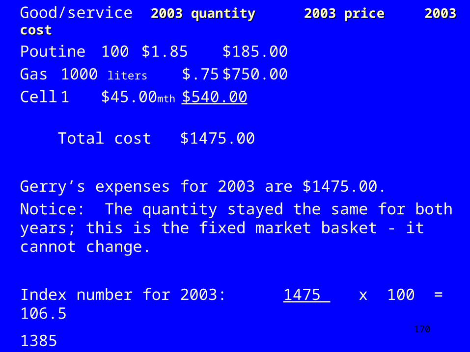
Good/service 2003 quantity 2003 price2003 quantity 2003 price 2003 2003 costcost

Poutine 100 $1.85 $185.00 Gas 1000 liters $.75 $750.00 Cell 1 $45.00mth $540.00 Total cost $1475.00

Gerry’s expenses for 2003 are $1475.00. Notice: The quantity stayed the same for both years;

this is the fixed market basket - it cannot change.

Index number for 2003: 1475 x 100 = 106.5 1385

171

Gerry’s index points rose 6.5% in two years.

The most famous index number for a fixed market basket of goods is the Consumer Price IndexConsumer Price Index.

It is also called inflation, or the percent increase for living expenses given a fixed basket.

Important that pensions be indexed to the CPI; go up as much as the CPI to not lose purchasing power.

CPI is used to establish the relative value of money (the purchasing power) for two different time periods.

172

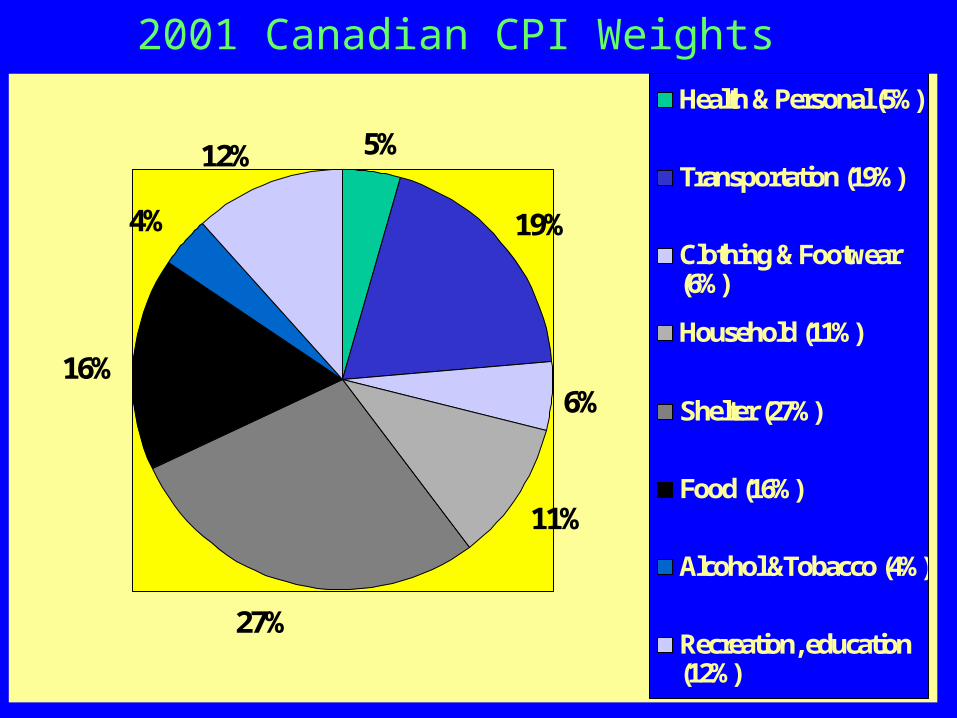
2001 Canadian CPI Weights

5%

19%

6%

11%

27%

16%

4%

12%

Health & Personal (5%)

Transportation (19%)

Clothing & Footwear(6%)

Household (11%)

Shelter (27%)

Food (16%)

Alcohol &Tobacco (4%)

Recreation, education(12%)

173

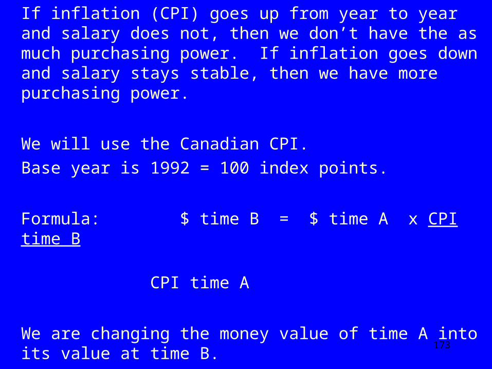
If inflation (CPI) goes up from year to year and salary does not, then we don’t have the as much purchasing power. If inflation goes down and salary stays stable, then we have more purchasing power.

We will use the Canadian CPI. Base year is 1992 = 100 index points.

Formula: $ time B = $ time A x CPI time B CPI time A

We are changing the money value of time A into its value at time B.

174

CANADIAN CONSUMER PRICE INDEX

YEAR CPI YEAR CPI YEAR CPI

1949 14.5 1969 23.4 1989 89.0

1950 14.9 1970 24.2 1990 93.3

1951 16.4 1971 24.9 1991 98.5

1952 16.9 1972 26.1 1992 100.0

1953 16.7 1973 28.1 1993 101.8

1954 16.8 1974 31.1 1994 102.0

1955 16.8 1975 34.5 1995 104.2

1956 17.1 1976 37.1 1996 105.9

1957 17.6 1977 40.0 1997 107.6

1958 18.0 1978 43.6 1998 108.6

1959 18.3 1979 47.6 1999 108.9

1960 18.5 1980 52.4 2000 111.4

1961 18.7 1981 58.9 2001 115.9

1962 18.9 1982 65.3 2 2002 120.4

1963 19.2 1983 69.1 2003 122.7

1964 19.6 1984 72.1 2004 125.1

1965 20.0 1985 75.0

1966 20.8 1986 78.1

1967 21.5 1987 81.5

1968 22.4 1988 84.8

Taken from: Canadian Economic Observer, Statistic Canada - Cat No. 11-210-XPB,1997/1998 and http://www.bankofcanada.ca/en/inflation_calc.htm visited: January 21, 2004

175

Example: A person makes $120 per week in 1998. What salary would it take to have the same

purchasing power in 2003.

$ time 2003 = $120.00 x 122.7 = $135.58 108.6

If salary did not increase during those years: $120 x 52 = $6240 (1998) $135,58 x 52 = $7050.17. (2003) Lost $810.17 in purchasing power in the 2003 year.

This does not take into account the loss of purchasing power in the previous years.

176

Example 2: An apartment cost $450 in 2000. In 2003 that

apartment cost $650. Calculate what the apartment would have cost if inflation were the only rent increase factor.

$ time 2003 = $450 x 122.7 = $495.65 111.4

In 2003, the apartment costs $650; given inflation it should cost $495.65.

The difference, $154.35, is due to ‘supply and demand’ factors.

Bank of Canada: Calculation Web page

177

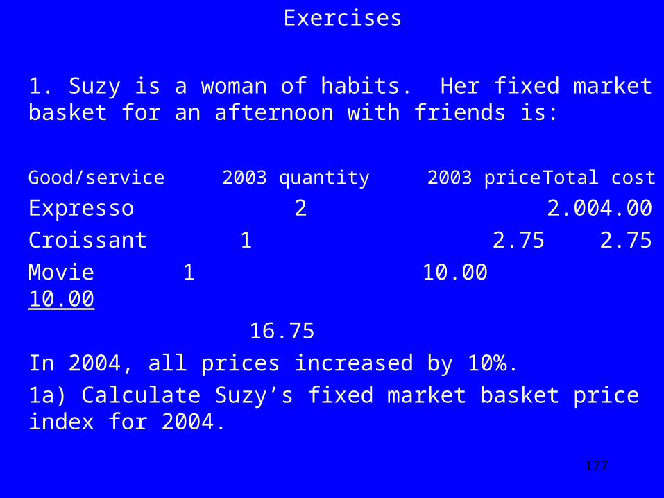
Exercises

1. Suzy is a woman of habits. Her fixed market basket for an afternoon with friends is:

Good/service 2003 quantity 2003 price Total cost

Expresso 2 2.00 4.00 Croissant 1 2.75 2.75 Movie 1 10.00 10.00 16.75 In 2004, all prices increased by 10%. 1a) Calculate Suzy’s fixed market basket price index

for 2004.

178

2. If a person earned $10.00 per hour in 1980, how much would they have to earn in 2002 to keep the same purchasing power?

179

3. In 2001, the minimum wage in Quebec was $7.00. How much would you have to earn in 2004 to keep the

same purchasing power?