Embed Size (px)
Citation preview
1
Shape Classification Using the Inner-Distance
Haibin Ling David W. Jacobs
Center for Automation Research and Computer Science Department
University of Maryland, College Park
{hbling, djacobs}@ umiacs.umd.edu
Abstract
Part structure and articulation are of fundamental importance in computer and human vision. We
propose using the inner-distance to build shape descriptors that are robust to articulation and capture
part structure. The inner-distance is defined as the length of the shortest path between landmark points
within the shape silhouette. We show that it is articulation insensitive and more effective at capturing part
structures than the Euclidean distance. This suggests that the inner-distance can be used as a replacement
for the Euclidean distance to build more accurate descriptors for complex shapes, especially for those
with articulated parts. In addition, texture information along the shortest path can be used to further
improve shape classification. With this idea, we propose three approaches to using the inner-distance.
The first method combines the inner-distance and multidimensional scaling (MDS) to build articulation
invariant signatures for articulated shapes. The second method uses the inner-distance to build a new
shape descriptor based on shape contexts. The third one extends the second one by considering the
texture information along shortest paths. The proposed approaches have been tested on a variety of
shape databases including an articulated shape dataset, MPEG7 CE-Shape-1, Kimia silhouettes, the
ETH-80 data set, two leaf data sets, and a human motion silhouette dataset. In all the experiments, our
methods demonstrate effective performance compared with other algorithms.
Index Terms
Computer vision, invariants, object recognition, shape, shape distance, texture, articulation
I. I NTRODUCTION
Part structure plays a very important role in classifying complex shapes in both human vision
and computer vision [21], [6], [23] etc. However, capturing part structure is not a trivial task,
2
especially considering articulations, which are nonlinear transformations between shapes. To
make things worse, sometimes shapes can have ambiguous parts (e.g. [4]). Unlike many previous
methods that deal with part structure explicitly, we propose an implicit approach to this task.
In this paper we introduce theinner-distance, defined as the length of the shortest path
within the shape boundary, to build shape descriptors. It is easy to see that the inner-distance
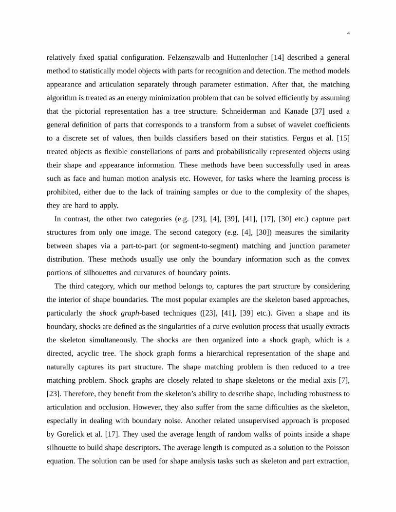
is insensitive to shape articulations. For example, in Fig. 1, although the points on shape (a)
and (c) have similar spatial distributions, they are quite different in their part structures. On the
other hand, shapes (b) and (c) appear to be from the same category with different articulations.
The inner-distance between the two marked points is quite different in (a) and (b), while almost
the same in (b) and (c). Intuitively, this example shows that the inner-distance is insensitive to
articulation and sensitive to part structures, a desirable property for complex shape comparison.
Note that the Euclidean distance does not have these properties in this example. This is because,
defined as the length of the line segment between landmark points, the Euclidean distance does
not consider whether the line segment crosses shape boundaries. In this example, it is clear that
the inner-distance reflects part structure and articulation without explicitly decomposing shapes
into parts. We will study this problem in detail and give more examples in the following sections.
Fig. 1. Three objects. The dashed lines denote shortest paths within the shape boundary that connect landmark points.
It is natural to use the inner-distance as a replacement for other distance measures to build
new shape descriptors that are invariant/insensitive to articulation. In this paper we propose and
experiment with two approaches. In the first approach, by replacing the geodesic distance with the
inner-distance, we extend the bending invariant signature for 3D surfaces [12] to the articulation
invariant signature for 2D articulated shapes. In the second method, the inner-distance replaces
the Euclidean distance to extend the shape context [5]. We design a dynamic programming
method for silhouette matching that is fast and accurate since it utilizes the ordering information
between contour points. Both approaches are tested on a variety of shape databases, including an
3
articulated shape database1, MPEG7 CE-Shape-1 shapes, Kimia’s silhouette [40], [39], ETH-80
[26], a Swedish leaf database [42] and a Smithsonian leaf database [2]. The excellent performance
demonstrates the inner-distance’s ability to capture part structures (not just articulations).
In practice, it is often desirable to combine shape and texture information for object recogni-
tion. For example, leaves from different species often share similar shapes but have different vein
structures (see Fig. 13 for examples). Using the gradient information along the shortest path, we
propose a new shape descriptor that naturally takes into account the texture information inside
a given shape. The new descriptor is applied to a foliage image task and excellent performance
is observed.
The rest of this paper is organized as follows. Sec. II discusses related works. Sec. III first
gives the definition of the inner-distance and its computation. Then the articulation insensitivity
of the inner-distance is proved. After that we address the inner-distance’s ability to capture part
structures. Sec. IV describes using the inner-distance and MDS to build articulation insensitive
signatures for 2D articulated shapes. Sec. V describes the extension of the shape context using the
inner-distance, and gives a framework for using dynamic programming for silhouette matching
and comparison. Sec. VI introduces the new shape descriptor that captures texture information.
Sec. VII presents and analyzes all experiments. Sec. VIII concludes the paper.
II. RELATED WORK
A. Representation and Comparison of Shapes with Parts and Articulation
For general shape matching, a recent review is given in [45]. Roughly speaking, works handling
parts can be classified into three categories. The first category (e.g. [3], [19], [14], [37], [15], [46]
etc.) builds part models from a set of sample images, and usually with some prior knowledge
such as the number of parts. After that, the models are used for retrieval tasks such as object
recognition and detection. These works usually use statistical methods to describe the articulation
between parts and often require a learning process to find the model parameters. For example,
Grimson [19] proposed some early work performing matching with precise models of articulation.
Agarwal et al. [3] proposed a framework for object detection via learning sparse, part-based
representations. The method is targeted to objects that consist of distinguishable parts with
1This is a dataset we collected and available at http://www.cs.umd.edu/∼hbling/Research/data/articu.zip
4
relatively fixed spatial configuration. Felzenszwalb and Huttenlocher [14] described a general
method to statistically model objects with parts for recognition and detection. The method models
appearance and articulation separately through parameter estimation. After that, the matching
algorithm is treated as an energy minimization problem that can be solved efficiently by assuming
that the pictorial representation has a tree structure. Schneiderman and Kanade [37] used a
general definition of parts that corresponds to a transform from a subset of wavelet coefficients
to a discrete set of values, then builds classifiers based on their statistics. Fergus et al. [15]
treated objects as flexible constellations of parts and probabilistically represented objects using
their shape and appearance information. These methods have been successfully used in areas
such as face and human motion analysis etc. However, for tasks where the learning process is
prohibited, either due to the lack of training samples or due to the complexity of the shapes,
they are hard to apply.
In contrast, the other two categories (e.g. [23], [4], [39], [41], [17], [30] etc.) capture part
structures from only one image. The second category (e.g. [4], [30]) measures the similarity
between shapes via a part-to-part (or segment-to-segment) matching and junction parameter
distribution. These methods usually use only the boundary information such as the convex
portions of silhouettes and curvatures of boundary points.
The third category, which our method belongs to, captures the part structure by considering
the interior of shape boundaries. The most popular examples are the skeleton based approaches,
particularly theshock graph-based techniques ([23], [41], [39] etc.). Given a shape and its
boundary, shocks are defined as the singularities of a curve evolution process that usually extracts
the skeleton simultaneously. The shocks are then organized into a shock graph, which is a
directed, acyclic tree. The shock graph forms a hierarchical representation of the shape and
naturally captures its part structure. The shape matching problem is then reduced to a tree
matching problem. Shock graphs are closely related to shape skeletons or the medial axis [7],
[23]. Therefore, they benefit from the skeleton’s ability to describe shape, including robustness to
articulation and occlusion. However, they also suffer from the same difficulties as the skeleton,
especially in dealing with boundary noise. Another related unsupervised approach is proposed
by Gorelick et al. [17]. They used the average length of random walks of points inside a shape
silhouette to build shape descriptors. The average length is computed as a solution to the Poisson
equation. The solution can be used for shape analysis tasks such as skeleton and part extraction,
5
local orientation detection, shape classification, etc.
The inner-distance is closely related to the skeleton based approaches in that it also considers
the interior of the shape. Given two landmark points, the inner-distance can be “approximated”
by first finding their closest points on the shape skeleton, then measuring the distance along the
skeleton. In fact, the inner-distance can also be computed via the evolution equations starting
from boundary points. The main difference between the inner-distance and the skeleton based
approaches is that the inner-distance discards the structure of the path once their lengths are
computed. By doing this, the inner-distance is more robust to disturbances along boundaries
and becomes very flexible for building shape descriptors. For example, it can be easily used
to extend existing descriptors by replacing Euclidean distances. In addition, the inner-distance
based descriptors can be used for landmark point matching. This is very important for some
applications such as motion analysis. The disadvantage is the loss of the ability to perform part
analysis. It is an interesting future work to see how to combine the inner-distance and skeleton
based techniques.
B. Geodesic Distances for 3D Surfaces
The inner-distance is very similar to the geodesic distance on surfaces. The geodesic distances
between any pair of points on a surface is defined as the length of the shortest path on the surface
between them. One of our motivations comes from Elad and Kimmel’s work [12] using geodesic
distances for 3D surface comparison through multidimensional scaling (MDS). Given a surface
and sample points on it, the surface is distorted using MDS, so that the Euclidean distances
between the stretched sample points are as similar as possible to their corresponding geodesic
distances on the original surface. Since the geodesic distance is invariant to bending, the stretched
surface forms a bending invariant signature of the original surface.
Bending invariance is quite similar to the 2D articulation invariance in which we are interested.
However, the direct counterpart of the geodesic distance in 2D does not work for our purpose.
Strictly speaking, the geodesic distance between two points on the “surface” of a 2D shape is the
distance between them along the contour. If a simple (i.e. non self-intersecting), closed contour
has lengthM , then for any point,p, and anyd < M/2, there will be exactly two pointsq1, q2 that
are a distanced away fromp, along the contour (see Fig. 2 for examples). Hence, a histogram
of the geodesic distance to all points on the contour degenerates into something trivial, which
6
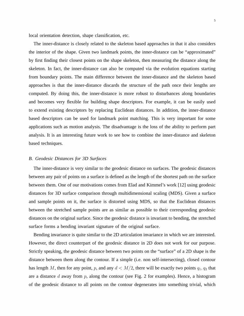
does not capture shape. Unlike the geodesic distance, the inner-distance measures the length of
the shortest path within the shape boundary instead of along the shape contour (surface). We
will show that the inner distance is very informative and insensitive to articulation.
Fig. 2. Geodesic distances on 2D shapes. Using the geodesic distances along the contours, the two shapes are indistinguishable.
There are other works using geodesic distances in shape descriptions. For example, Hamza and
Krim [20] applied geodesic distance usingshape distributions([35]) for 3D shape classification.
Zhao and Davis [48] used the color information along the shortest path within a human silhouette.
The articulation invariance of shortest paths is also utilized by them, but in the context of
background subtraction. Ling and Jacobs [28] proposed using the geodesic distance to achieve
deformation invariance in intensity images. A preliminary version of this paper appeared as [29].
C. Shape Contexts for 2D Shapes
The shape contextwas introduced by Belongie et al. [5]. It describes the relative spatial
distribution (distance and orientation) of landmark points around feature points. Givenn sample
pointsx1, x2, ..., xn on a shape, the shape context at pointxi is defined as a histogramhi of the
relative coordinates of the remainingn− 1 points
hi(k) = #{xj : j 6= i, xj − xi ∈ bin(k)} (1)
where the bins uniformly divide the log-polar space. The distance between two shape context
histograms is defined using theχ2 statistic.
For shape comparison, Belongie et al. used a framework combining shape context and thin-
plate-splines [8] (SC+TPS). Given the points on two shapesA andB, first the point correspon-
dences are found through a weighted bipartite matching. Then, TPS is used iteratively to estimate
the transformation between them. After that, the similarityD betweenA andB is measured as
a weighted combination of three parts
D = aDac + Dsc + bDbe (2)

7
whereDac measures the appearance difference.Dbe measures the bending energy. TheDsc term,
named theshape context distance, measures the average distance between a point onA and its
most similar counterpart onB (in the sense of (10)).a, b are weights (a = 1.6, b = 0.3 in [5]).
The shape context uses the Euclidean distance to measure the spatial relation between landmark
points. This causes less discriminability for complex shapes with articulations (e.g., Fig. 8 and
9). The inner-distance is a natural way to solve this problem since it captures the shape structure
better than the Euclidean distance. We use the inner-distance to extend the shape context for
shape matching. The advantages of the new descriptor are strongly supported by experiments.
Belongie et al. showed that the SC+TPS is very effective for shape matching tasks. Due
to its simplicity and discriminability, the shape context has become quite popular recently.
Some examples can be found in [33], [43], [44], [47], [34], [26]. Among these works, [43] is
most related to our approach. Thayananthan et al. [43] suggested including a figural continuity
constraint for shape context matching via an efficient dynamic programming scheme. In our
approach, we also include a similar constraint by assuming that contour points are ordered and
use dynamic programming for matching the shape context at contour sample points. Notice that
usually dynamic programming encounters problems with shapes with multiple boundaries (e.g.,
scissors with holes). The inner-distance has no such problem since it only requires landmark
points on the outermost silhouette, and the shortest path can be computed taking account of
holes. This will be discussed in the following sections.
III. T HE INNER-DISTANCE
In this section, we will first give the definition of the inner-distance and discuss how to
compute it. Then, the inner-distance’s insensitivity to part articulations is proven. After that, we
will discuss its ability to capture part structures.
A. The Inner-Distance and Its Computation
First, we define a shapeO as a connected and closed subset ofR2. Given a shapeO and two
pointsx, y ∈ O, the inner-distance betweenx, y, denoted asd(x, y; O), is defined as the length
of the shortest path connectingx andy within O. One example is shown in Fig. 3.
Note: 1) There may exist multiple shortest paths between given points. However, for most
cases, the path is unique. In rare cases where there are multiple shortest paths, we arbitrarily

8
choose one. 2) We are interested in shapes defined by their boundaries, hence only boundary
points are used as landmark points. In addition, we approximate a shape with a polygon formed
by their landmark points.
Fig. 3. Definition of the inner-distance. The dashed polyline shows the shortest path between pointx andy.
A natural way to compute the inner-distance is using shortest path algorithms. It consists of
two steps:
1) Build a graph with the sample points. First, each sample point is treated as a node in the
graph. Then, for each pair of sample pointsp1 andp2, if the line segment connectingp1
and p2 falls entirely within the object, an edge betweenp1 and p2 is added to the graph
with its weight equal to the Euclidean distance‖p1− p2‖. An example is shown in Fig. 4.
Note 1) Neighboring boundary points are always connected; 2) The inner-distance reflects
the existence of holes without using sample points from hole boundaries2, which allows
dynamic programming algorithms to be applied to shapes with holes.
2) Apply a shortest path algorithm to the graph. Many standard algorithms [11] can be applied
here, among them Johnson or Floyd-Warshall’s algorithms haveO(n3) complexity (n is
the number of sample points).
In this paper we are interested in the inner-distance between all pairs of points. Now we
will show that this can be computed withO(n3) time complexity forn sample points. First,
it takes timeO(n) to check whether a line segment between two points is inside the given
shape (by checking the intersections between linep1p2 and all other boundary line segments,
with several extra tests). As a result, the complexity of graph construction is ofO(n3). After
the graph is ready, the all-pair shortest path algorithm has complexity ofO(n3). Therefore, the
whole computation takesO(n3).
2The points along hole boundaries may still be needed for computing the inner-distance, but not for building descriptors.
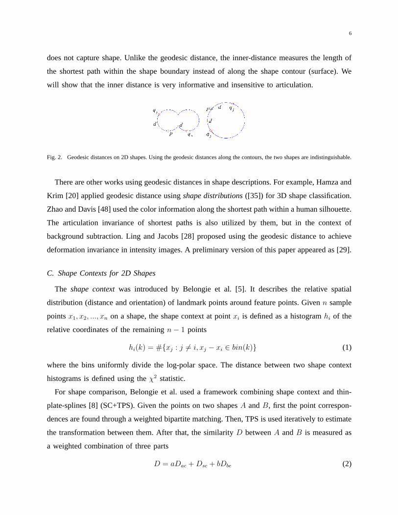
9
Fig. 4. Computation of the inner-distance. Left, the shape with the sampled silhouette landmark points. Middle, the graph built
using the landmark points. Right, a detail of the right top of the graph. Note how the inner-distance captures the holes.
Note that whenO is convex, the inner-distance reduces to the Euclidean distance. However,
this is not always true for non-convex shapes (e.g., Fig. 1). This suggests that the inner-distance
is influenced by part structure to which the concavity of contours is closely related [21], [13].
In the following subsections, we discuss this in detail.
B. Articulation Insensitivity of the Inner-Distance
As shown in Fig. 1, the inner-distance is insensitive to articulation. Intuitively, this is true
because an articulated shape can be decomposed into rigid parts connected by junctions. Ac-
cordingly, the shortest path between landmark points can be divided into segments within each
parts. We will first give a very general model for part articulation and then formally prove
articulation insensitivity of the inner-distance.
1) A Model of Articulated Objects:Before discussing the articulation insensitivity of the
inner-distance, we need to provide a model of articulated objects. Note that our method does
not involve any part models, the model here is only for the analysis of the properties of the
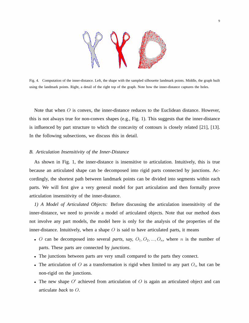
inner-distance. Intuitively, when a shapeO is said to have articulated parts, it means
• O can be decomposed into severalparts, say, O1, O2, ..., On, wheren is the number of
parts. These parts are connected byjunctions.
• The junctions between parts are very small compared to the parts they connect.
• The articulation ofO as a transformation is rigid when limited to any partOi, but can be
non-rigid on the junctions.
• The new shapeO′ achieved from articulation ofO is again an articulated object and can
articulateback to O.
10
Based on these intuition, we define an articulated objectO ⊂ R2 of n parts together with an
articulationf as:
O = {n⋃
i=1
Oi}⋃{⋃
i6=j
Jij}
where
• ∀i, 1≤i≤n, part Oi⊂R2 is connected and closed, andOi⋂
Oj = Ø, ∀i6=j, 1≤i, j≤n.
• ∀i6=j, 1≤i, j≤n, Jij⊂R2, connected and closed, is the junction betweenOi andOj. If there
is no junction betweenOi andOj, thenJij = Ø. Otherwise,Jij⋂
Oi 6=Ø, Jij⋂
Oj 6=Ø.
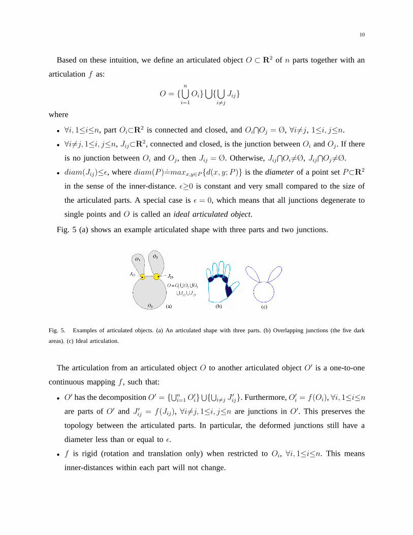
• diam(Jij)≤ε, wherediam(P ).=maxx,y∈P{d(x, y; P )} is thediameterof a point setP⊂R2
in the sense of the inner-distance.ε≥0 is constant and very small compared to the size of
the articulated parts. A special case isε = 0, which means that all junctions degenerate to
single points andO is called anideal articulated object.
Fig. 5 (a) shows an example articulated shape with three parts and two junctions.
Fig. 5. Examples of articulated objects. (a) An articulated shape with three parts. (b) Overlapping junctions (the five dark
areas). (c) Ideal articulation.
The articulation from an articulated objectO to another articulated objectO′ is a one-to-one
continuous mappingf , such that:
• O′ has the decompositionO′ = {⋃ni=1 O′
i}⋃{⋃i 6=j J ′ij}. Furthermore,O′
i = f(Oi), ∀i, 1≤i≤n
are parts ofO′ and J ′ij = f(Jij), ∀i 6=j, 1≤i, j≤n are junctions inO′. This preserves the
topology between the articulated parts. In particular, the deformed junctions still have a
diameter less than or equal toε.
• f is rigid (rotation and translation only) when restricted toOi, ∀i, 1≤i≤n. This means
inner-distances within each part will not change.
11
Notes: 1) In the above and following, we use the notationf(P ).= {f(x) : x ∈ P} for short. 2)
It is obvious from the above definitions thatf−1 is an articulation that mapsO′ to O.
The above model of articulation is very general and flexible. For example, there is no restriction
on the shape of the junctions. Junctions are even allowed to overlap each other. Furthermore,
the articulationf on the junctions are not required to be smooth. Fig. 5 (b) and (c) gives two
more examples of articulated shapes.
2) Articulation Insensitivity:We are interested in how the inner-distance varies under articu-
lation. From previous paragraphs we know that changes of the inner-distance are due to junction
deformations. Intuitively, this means the change is very small compared to the size of parts. Since
most pairs of points have inner-distances comparable to the sizes of parts, the relative change of
the inner-distances during articulation are small. This roughly explains why the inner-distances
are articulation insensitive.
We will use following notations: 1)Γ(x1, x2; P ) denotes a shortest path fromx1∈P to x2∈P
for a closed and connected point setP⊂R2 (so d(x1, x2; P ) is the length ofΓ(x1, x2; P )). 2) ′
indicates the image of a point or a point set underf , e.g.,P ′ .=f(P ) for point setP , p′ .=f(p)
for a pointp. 3) “[” and “]” denote the concatenation of paths.
Let us first point out two facts about the inner-distance within a part or crossing a junction.
Both facts are direct results from the definitions in sec. III-B.1.
d(x, y; Oi) = d(x′, y′; O′i) , ∀x, y∈Oi, 1≤i≤n (3)
|d(x, y; O)− d(x′, y′; O′)| ≤ ε ,
∀x, y ∈ Jij, ∀i 6=j, 1≤i, j≤n, Jij 6= Ø(4)
Note that (4) does not require the shortest path betweenx, y to lie within the junctionJij. These
two facts describe the change of the inner-distances of restricted point pairs. For the general
case ofx, y∈O, we have the following theorem:
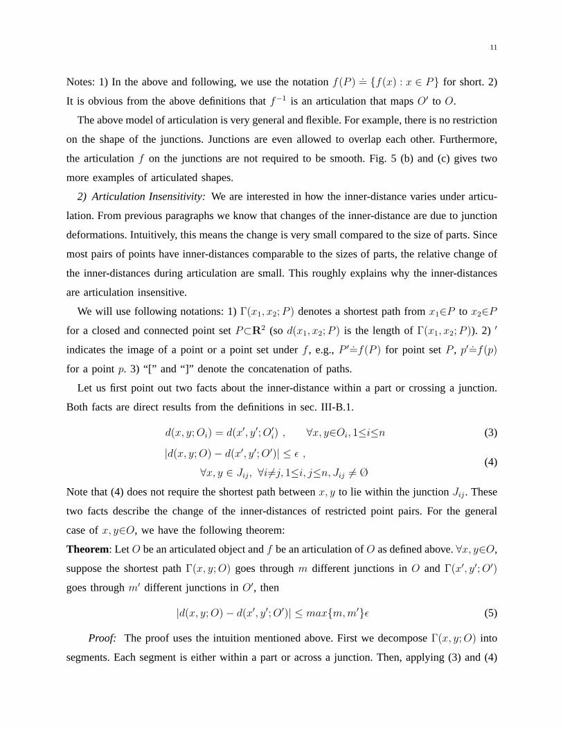
Theorem: Let O be an articulated object andf be an articulation ofO as defined above.∀x, y∈O,
suppose the shortest pathΓ(x, y; O) goes throughm different junctions inO and Γ(x′, y′; O′)
goes throughm′ different junctions inO′, then
|d(x, y; O)− d(x′, y′; O′)| ≤ max{m,m′}ε (5)
Proof: The proof uses the intuition mentioned above. First we decomposeΓ(x, y; O) into
segments. Each segment is either within a part or across a junction. Then, applying (3) and (4)

12
to each segment leads to the theorem.
First, Γ(x, y; O) is decomposed intol segments:
Γ(x, y; O) = [Γ(p0, p1; R1), Γ(p1, p2; R2), ..., Γ(pl−1, pl; Rl)]
using point sequencep0, p1, ..., pl and regionsR1, ..., Rl via the steps using Algorithm 1.
Algorithm 1 DecomposeΓ(x, y; O)
p0←x, i←0
while pi 6=y do {/*find pi+1*/}i←i + 1
Ri ← the region (a part or a junction)Γ(x, y; O) enters afterpi−1
if Ri = Ok for somek (Ri is a part)then {/*enter a part*/}Setpi as a point inOk such that
1) Γ(pi−1, pi; Ok) ⊆ Γ(x, y; O)
2) Γ(x, y; O) enters a new region (a part or a junction) afterpi or pi = y
else{/*Ri = Jrs for somer, s (Ri is a junction), enter a junction*/}Setpi as the point inJrs
⋂Γ(x, y; O) such thatΓ(x, y; O) never re-entersJrs after pi.
Ri ← the union of all the parts and junctionsΓ(pi−1, pi; O) passes through (noteJrs⊆Ri).
end if
end while
l←i
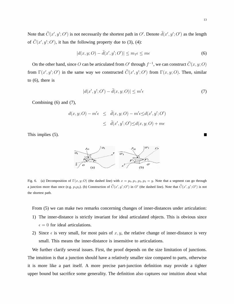
An example of this decomposition is shown in Fig. 6 (a). With this decomposition,d(x, y; O)
can be written as:
d(x, y; O) =∑
1≤i≤ld(pi−1, pi; Ri)
Supposem1 of the segments cross junctions (i.e., segments not contained in any single part),
then obviouslym1≤m.
In O′, we construct a path fromx′ to y′ corresponding toΓ(x, y; O) as follows (e.g. Fig. 6
(b)):
C(x′, y′; O′)=[Γ(p′0, p′1; R
′1), Γ(p′1, p
′2; R
′2), ..., Γ(p′l−1, p
′l; R
′l)]
13
Note thatC(x′, y′; O′) is not necessarily the shortest path inO′. Denoted(x′, y′; O′) as the length
of C(x′, y′; O′), it has the following property due to (3), (4):
|d(x, y; O)− d(x′, y′; O′)| ≤ m1ε ≤ mε (6)
On the other hand, sinceO can be articulated fromO′ throughf−1, we can constructC(x, y; O)
from Γ(x′, y′; O′) in the same way we constructedC(x′, y′; O′) from Γ(x, y; O). Then, similar
to (6), there is
|d(x′, y′; O′)− d(x, y; O)| ≤ m′ε (7)
Combining (6) and (7),
d(x, y; O)−m′ε ≤ d(x, y; O)−m′ε≤d(x′, y′; O′)
≤ d(x′, y′; O′)≤d(x, y; O) + mε
This implies (5).
Fig. 6. (a) Decomposition ofΓ(x, y; O) (the dashed line) withx = p0, p1, p2, p3 = y. Note that a segment can go through
a junction more than once (e.g.p1p2). (b) Construction ofC(x′, y′; O′) in O′ (the dashed line). Note thatC(x′, y′; O′) is not
the shortest path.
From (5) we can make two remarks concerning changes of inner-distances under articulation:
1) The inner-distance is strictly invariant for ideal articulated objects. This is obvious since
ε = 0 for ideal articulations.
2) Sinceε is very small, for most pairs ofx, y, the relative change of inner-distance is very
small. This means the inner-distance is insensitive to articulations.
We further clarify several issues. First, the proof depends on the size limitation of junctions.
The intuition is that a junction should have a relatively smaller size compared to parts, otherwise
it is more like a part itself. A more precise part-junction definition may provide a tighter
upper bound but sacrifice some generality. The definition also captures our intuition about what
14
distinguishes articulation from deformation. Second, the part-junction model is not actually used
at all when applying the inner-distance. In fact, one advantage of using the inner-distance is that
it implicitly captures part structure, whose definition is still not clear in general.
C. Inner-Distances and Part Structures
In addition to articulation insensitivity, we believe that the inner-distance captures part struc-
tures better than the Euclidean distance. This is hard to prove because the definition of part
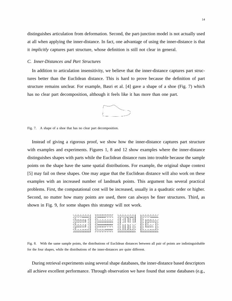
structure remains unclear. For example, Basri et al. [4] gave a shape of a shoe (Fig. 7) which
has no clear part decomposition, although it feels like it has more than one part.
Fig. 7. A shape of a shoe that has no clear part decomposition.
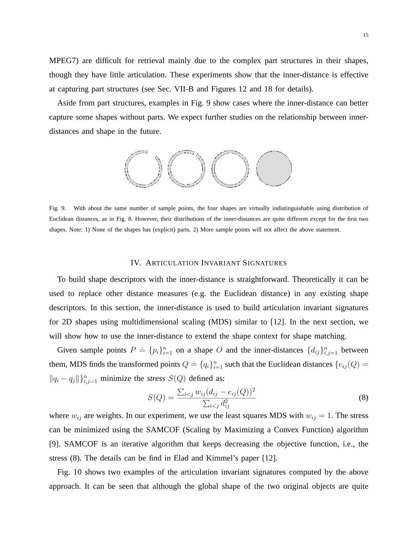
Instead of giving a rigorous proof, we show how the inner-distance captures part structure
with examples and experiments. Figures 1, 8 and 12 show examples where the inner-distance
distinguishes shapes with parts while the Euclidean distance runs into trouble because the sample
points on the shape have the same spatial distributions. For example, the original shape context
[5] may fail on these shapes. One may argue that the Euclidean distance will also work on these
examples with an increased number of landmark points. This argument has several practical
problems. First, the computational cost will be increased, usually in a quadratic order or higher.
Second, no matter how many points are used, there can always be finer structures. Third, as
shown in Fig. 9, for some shapes this strategy will not work.
Fig. 8. With the same sample points, the distributions of Euclidean distances between all pair of points are indistinguishable
for the four shapes, while the distributions of the inner-distances are quite different.
During retrieval experiments using several shape databases, the inner-distance based descriptors
all achieve excellent performance. Through observation we have found that some databases (e.g.,
15
MPEG7) are difficult for retrieval mainly due to the complex part structures in their shapes,
though they have little articulation. These experiments show that the inner-distance is effective
at capturing part structures (see Sec. VII-B and Figures 12 and 18 for details).
Aside from part structures, examples in Fig. 9 show cases where the inner-distance can better
capture some shapes without parts. We expect further studies on the relationship between inner-
distances and shape in the future.
Fig. 9. With about the same number of sample points, the four shapes are virtually indistinguishable using distribution of
Euclidean distances, as in Fig. 8. However, their distributions of the inner-distances are quite different except for the first two
shapes. Note: 1) None of the shapes has (explicit) parts. 2) More sample points will not affect the above statement.
IV. A RTICULATION INVARIANT SIGNATURES
To build shape descriptors with the inner-distance is straightforward. Theoretically it can be
used to replace other distance measures (e.g. the Euclidean distance) in any existing shape
descriptors. In this section, the inner-distance is used to build articulation invariant signatures
for 2D shapes using multidimensional scaling (MDS) similar to [12]. In the next section, we
will show how to use the inner-distance to extend the shape context for shape matching.
Given sample pointsP .= {pi}n
i=1 on a shapeO and the inner-distances{dij}ni,j=1 between
them, MDS finds the transformed pointsQ.= {qi}n
i=1 such that the Euclidean distances{eij(Q) =
‖qi − qj‖}ni,j=1 minimize thestressS(Q) defined as:
S(Q) =
∑i<j wij(dij − eij(Q))2
∑i<j d2
ij
(8)
wherewij are weights. In our experiment, we use the least squares MDS withwij = 1. The stress
can be minimized using the SAMCOF (Scaling by Maximizing a Convex Function) algorithm
[9]. SAMCOF is an iterative algorithm that keeps decreasing the objective function, i.e., the
stress (8). The details can be find in Elad and Kimmel’s paper [12].
Fig. 10 shows two examples of the articulation invariant signatures computed by the above
approach. It can be seen that although the global shape of the two original objects are quite
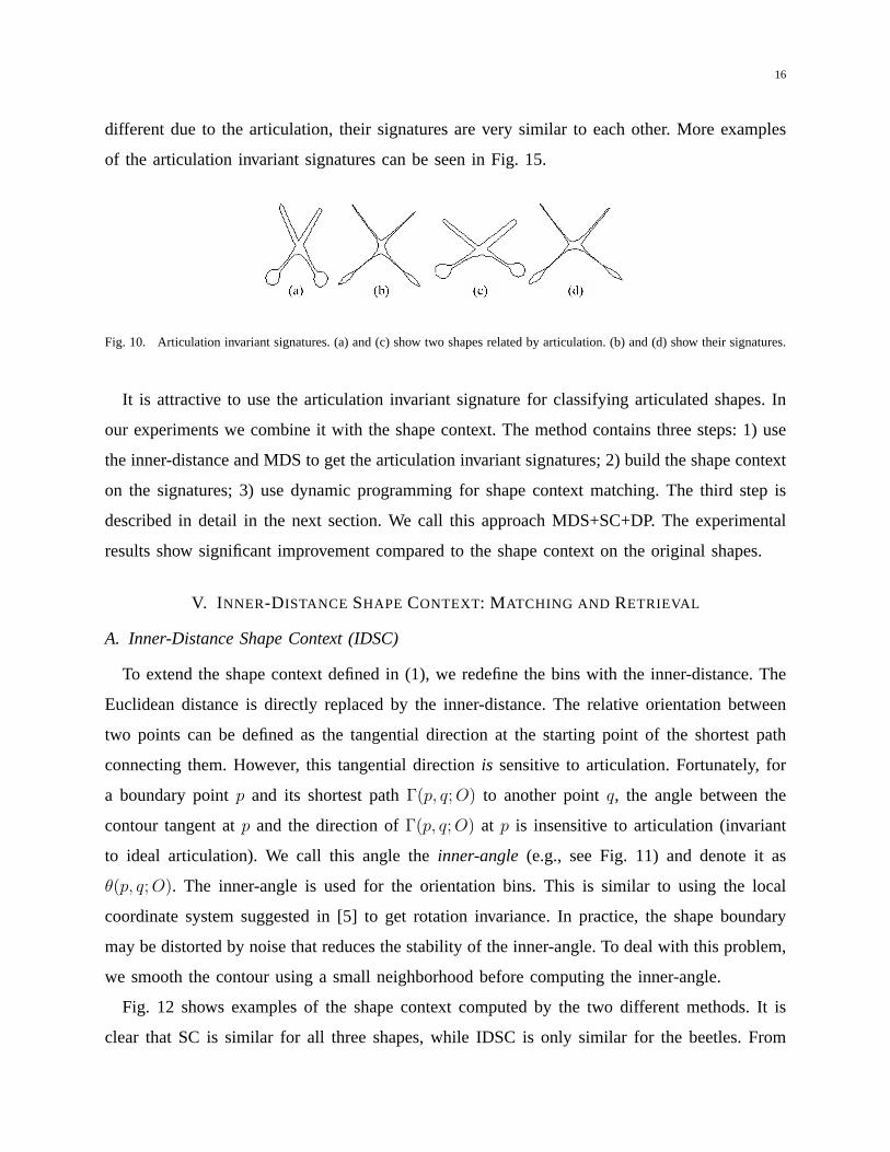
16
different due to the articulation, their signatures are very similar to each other. More examples
of the articulation invariant signatures can be seen in Fig. 15.
Fig. 10. Articulation invariant signatures. (a) and (c) show two shapes related by articulation. (b) and (d) show their signatures.
It is attractive to use the articulation invariant signature for classifying articulated shapes. In
our experiments we combine it with the shape context. The method contains three steps: 1) use
the inner-distance and MDS to get the articulation invariant signatures; 2) build the shape context
on the signatures; 3) use dynamic programming for shape context matching. The third step is
described in detail in the next section. We call this approach MDS+SC+DP. The experimental
results show significant improvement compared to the shape context on the original shapes.
V. I NNER-DISTANCE SHAPE CONTEXT: MATCHING AND RETRIEVAL
A. Inner-Distance Shape Context (IDSC)
To extend the shape context defined in (1), we redefine the bins with the inner-distance. The
Euclidean distance is directly replaced by the inner-distance. The relative orientation between
two points can be defined as the tangential direction at the starting point of the shortest path
connecting them. However, this tangential directionis sensitive to articulation. Fortunately, for
a boundary pointp and its shortest pathΓ(p, q; O) to another pointq, the angle between the
contour tangent atp and the direction ofΓ(p, q; O) at p is insensitive to articulation (invariant
to ideal articulation). We call this angle theinner-angle (e.g., see Fig. 11) and denote it as
θ(p, q; O). The inner-angle is used for the orientation bins. This is similar to using the local
coordinate system suggested in [5] to get rotation invariance. In practice, the shape boundary
may be distorted by noise that reduces the stability of the inner-angle. To deal with this problem,
we smooth the contour using a small neighborhood before computing the inner-angle.
Fig. 12 shows examples of the shape context computed by the two different methods. It is
clear that SC is similar for all three shapes, while IDSC is only similar for the beetles. From

17
this figure we can see that the inner-distance is better at capturing parts than SC.
Fig. 11. The inner-angleθ(p, q; O) between two boundary points.
Fig. 12. Shape context (SC) and inner-distance shape context (IDSC). The top row shows three objects from the MPEG7 shape
database (Sec. VII-B), with two marked pointsp, q on each shape. The next rows show (from top to bottom), the SC atp, the
IDSC atp, the SC atq, the IDSC atq. Both the SC and the IDSC use local relative frames (i.e. aligned to the tangent). In the
histograms, the x axis denotes the orientation bins and the y axis denotes log distance bins.
The inner-angle is just a byproduct of the shortest path algorithms and does not affect the
complexity. Once the inner-distances and orientations between all pair of points are ready, it
takesO(n2) time to compute the histogram (1).
B. Shape Matching Through Dynamic Programming
The contour matching problem is formulated as follows: Given two shapesA andB, describe
them by point sequences on their contour, say,p1p2...pn for A with n points, andq1q2...qm for
B with m points. Without loss of generality, assumen ≥ m. The matchingπ from A to B is a
mapping from1, 2, ..., n to 0, 1, 2, ..., m, wherepi is matched toqπ(i) if π(i) 6= 0 and otherwise
left unmatched.π should minimize the match costH(π) defined as
C(π) =∑
1≤i≤nc(i, π(i)) (9)
wherec(i, 0) = τ is the penalty for leavingpi unmatched, and for1 ≤ j ≤ m, c(i, j) is the cost
of matchingpi to qj. This is measured using theχ2 statistic as in [5]
c(i, j)≡1
2
∑1≤k≤K
[hA,i(k)− hB,j(k)]2
hA,i(k) + hB,j(k)(10)

18
Here hA,i and hB,j are the shape context histograms ofpi and qj respectively, andK is the
number of histogram bins.
Since the contours provide orderings for the point sequencesp1p2...pn and q1q2...qm, it is
natural to restrict the matchingπ with this order. To this end, we use dynamic programming
(DP) to solve the matching problem. DP is widely used for contour matching. Detailed examples
can be found in [43], [4], [36]. We use the standard DP method [11] with the cost functions
defined as (9) and (10).
By default, the above method assumes the two contours are already aligned at their start and
end points. Without this assumption, one simple solution is to try different alignments at all
points on the first contour and choose the best one. The problem with this solution is that it
raises the matching complexity fromO(n2) to O(n3). Fortunately, for the comparison problem,
it is often sufficient to try aligning a fixed number of points, say,k points. Usuallyk is much
smaller thanm and n, this is because shapes can be first rotated according to their moments.
According to our experience, forn, m = 100, k = 4 or 8 is good enough and largerk does not
demonstrate significant improvement. Therefore, the complexity is stillO(kn2) = O(n2).
Bipartite graph matching is used in [5] to find the point correspondenceπ. Bipartite matching
is more general since it minimizes the matching cost (9) without additional constraints. For
example, it works when there is no ordering constraint on the sample points (while DP is not
applicable). For sequenced points along silhouettes, however, DP is more efficient and accurate
since it uses the ordering information provided by shape contours.
C. Shape Distances
Once the matching is found, we use the matching costC(π) as in (9) to measure the similarity
between shapes. One thing to mention is that dynamic programming is also suitable for shape
context. In the following, we use IDSC+DP to denote the method of using dynamic programming
matching with the IDSC, and use SC+DP for the similar method with the SC.
In addition to the excellent performance demonstrated in the experiments, the IDSC+DP
framework is simpler than the SC+TPS framework (2) [5]. First, besides the size of shape
context bins, IDSC+DP has only two parameters to tune: 1) The penaltyτ for a point with no
matching, usually set to 0.3, and 2) The number of start pointsk for different alignments during
the DP matching, usually set to 4 or 8. Second, IDSC+DP is easy to implement, since it does
19
not require the appearance and transformation model as well as the iteration and outlier control.
Furthermore, the DP matching is faster than bipartite matching, which is important for retrieval
in large shape databases.
The time complexity of the IDSC+DP consists of three parts. First, the computation of inner-
distances can be achieved inO(n3) with Johnson or Floyd-Warshall’s shortest path algorithms,
wheren is the number of sample points. Second, the construction of the IDSC histogram takes
O(n2). Third, the DP matching costsO(n2), and only this part is required for all pairs of shapes,
which is very important for retrieval tasks with large image databases. In our experiment using
partly optimized Matlab code on a regular Pentium IV 2.8G PC, a single comparison of two
shapes withn = 100 takes about 0.31 second.
VI. SHORTESTPATH TEXTURE CONTEXT
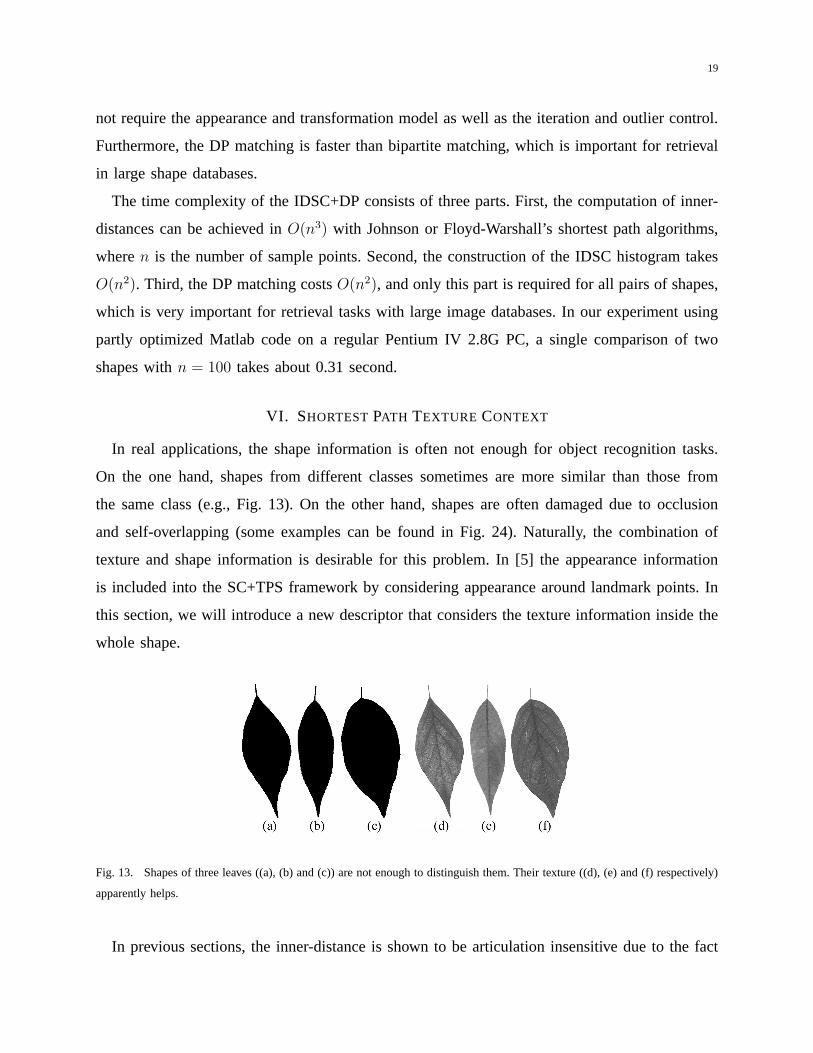
In real applications, the shape information is often not enough for object recognition tasks.
On the one hand, shapes from different classes sometimes are more similar than those from
the same class (e.g., Fig. 13). On the other hand, shapes are often damaged due to occlusion
and self-overlapping (some examples can be found in Fig. 24). Naturally, the combination of
texture and shape information is desirable for this problem. In [5] the appearance information
is included into the SC+TPS framework by considering appearance around landmark points. In
this section, we will introduce a new descriptor that considers the texture information inside the
whole shape.
Fig. 13. Shapes of three leaves ((a), (b) and (c)) are not enough to distinguish them. Their texture ((d), (e) and (f) respectively)
apparently helps.
In previous sections, the inner-distance is shown to be articulation insensitive due to the fact
20
that the shortest paths within shape boundaries are robust to articulation. Therefore, the texture
information along these paths provides a natural articulation insensitive texture description.
Note that this is true only when the paths are robust. In this section, we use local intensity
gradient orientations to capture texture information because of their robustness and efficiency.
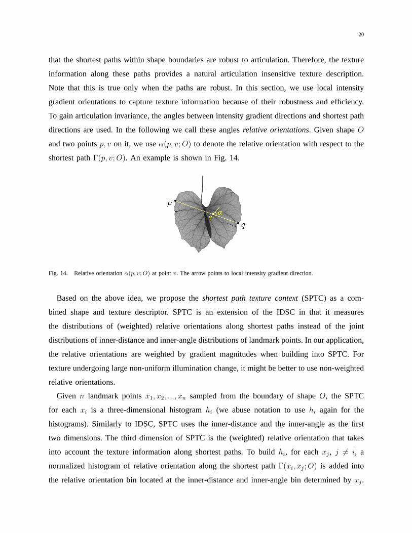
To gain articulation invariance, the angles between intensity gradient directions and shortest path
directions are used. In the following we call these anglesrelative orientations. Given shapeO
and two pointsp, v on it, we useα(p, v; O) to denote the relative orientation with respect to the
shortest pathΓ(p, v; O). An example is shown in Fig. 14.
Fig. 14. Relative orientationα(p, v; O) at pointv. The arrow points to local intensity gradient direction.
Based on the above idea, we propose theshortest path texture context(SPTC) as a com-
bined shape and texture descriptor. SPTC is an extension of the IDSC in that it measures
the distributions of (weighted) relative orientations along shortest paths instead of the joint
distributions of inner-distance and inner-angle distributions of landmark points. In our application,
the relative orientations are weighted by gradient magnitudes when building into SPTC. For
texture undergoing large non-uniform illumination change, it might be better to use non-weighted
relative orientations.
Given n landmark pointsx1, x2, ..., xn sampled from the boundary of shapeO, the SPTC
for eachxi is a three-dimensional histogramhi (we abuse notation to usehi again for the
histograms). Similarly to IDSC, SPTC uses the inner-distance and the inner-angle as the first
two dimensions. The third dimension of SPTC is the (weighted) relative orientation that takes
into account the texture information along shortest paths. To buildhi, for eachxj, j 6= i, a
normalized histogram of relative orientation along the shortest pathΓ(xi, xj; O) is added into
the relative orientation bin located at the inner-distance and inner-angle bin determined byxj.
21
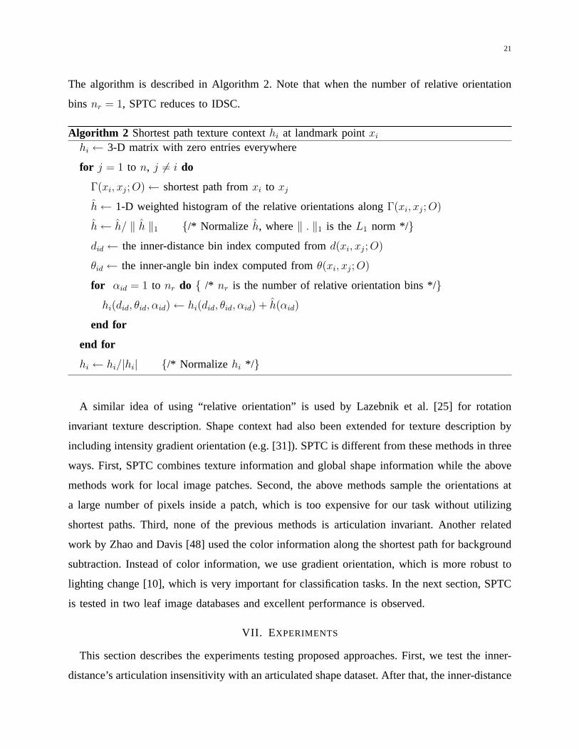
The algorithm is described in Algorithm 2. Note that when the number of relative orientation
bins nr = 1, SPTC reduces to IDSC.
Algorithm 2 Shortest path texture contexthi at landmark pointxi
hi ← 3-D matrix with zero entries everywhere
for j = 1 to n, j 6= i do
Γ(xi, xj; O) ← shortest path fromxi to xj
h ← 1-D weighted histogram of the relative orientations alongΓ(xi, xj; O)
h ← h/ ‖ h ‖1 {/* Normalize h, where‖ . ‖1 is theL1 norm */}did ← the inner-distance bin index computed fromd(xi, xj; O)
θid ← the inner-angle bin index computed fromθ(xi, xj; O)
for αid = 1 to nr do { /* nr is the number of relative orientation bins */}hi(did, θid, αid) ← hi(did, θid, αid) + h(αid)
end for
end for
hi ← hi/|hi| {/* Normalize hi */}
A similar idea of using “relative orientation” is used by Lazebnik et al. [25] for rotation
invariant texture description. Shape context had also been extended for texture description by
including intensity gradient orientation (e.g. [31]). SPTC is different from these methods in three
ways. First, SPTC combines texture information and global shape information while the above
methods work for local image patches. Second, the above methods sample the orientations at
a large number of pixels inside a patch, which is too expensive for our task without utilizing
shortest paths. Third, none of the previous methods is articulation invariant. Another related
work by Zhao and Davis [48] used the color information along the shortest path for background
subtraction. Instead of color information, we use gradient orientation, which is more robust to
lighting change [10], which is very important for classification tasks. In the next section, SPTC
is tested in two leaf image databases and excellent performance is observed.
VII. E XPERIMENTS
This section describes the experiments testing proposed approaches. First, we test the inner-
distance’s articulation insensitivity with an articulated shape dataset. After that, the inner-distance
22
is tested in comparison with other state-of-the-art approaches on several widely tested shape
data sets, including the MPEG7 CE-Shape-1 shapes, Kimia’s silhouette [40], [39], ETH-80 [26].
Then, the proposed approach is tested on two foliage image datasets, a Swedish leaf dataset
[42] and a Smithsonian leaf dataset. These experiments show how the inner-distance works in
real applications and how the SPTC performs on shapes with texture. Finally, we will show the
potential use of the IDSC on human motion analysis.
Now we describe the parameters used in the experiments. We usen to denote the number
of landmark points (on the outer contour of shapes). Landmark points are sampled uniformly
(as in [5]) to avoid bias.n is chosen according to the task. In general, largern will produce
greater accuracy with less efficiency. For the size of histograms,nd, nθ, and nr are used for
the number of inner-distance bins, the number of inner-angle bins, and the number of relative
orientation bins respectively. A typical setting for the bin number isnd = 5, nθ = 12 andnr = 8.
In our experiments, we sometimes usend = 8 to get better results. For dynamic programming,k
denotes the number of different starting points for alignment (uniformly chosen from landmark
points). The choice ofk was discussed in Sec. V-C. In general, a largerk increases the accuracy.
However in practice we found thatk = 4 − 8 usually gives satisfactory results. For example,
k = 8 is used for the MPEG7 dataset. However, we did notice that largerk can improve the
performance further, e.g.,k = 16 is used for the ETH-80 dataset that involves wildly varied
rotations. We did not rotate shapes according to their moments, which might be helpful for tasks
involving a large variation in orientations. The penaltyτ for one occlusion is always set to be
0.3 (our experiments show that differentτ in the range of[0.25, 0.5] do not affect the results too
much). In all the experiments, the parameters for MDS+SC+DP are the same as in IDSC+DP.
Furthermore, for datasets that have no previously reported shape context matching results, we
run the SC+DP for comparison with the same parameters as IDSC+DP.
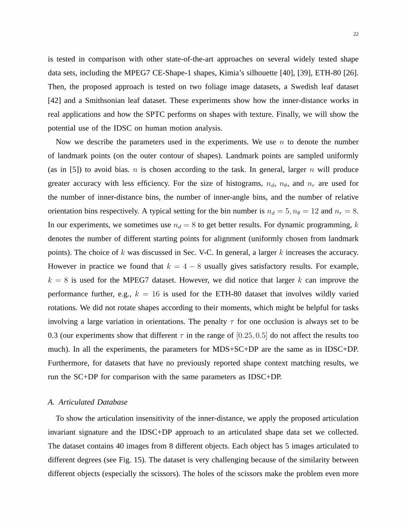
A. Articulated Database
To show the articulation insensitivity of the inner-distance, we apply the proposed articulation
invariant signature and the IDSC+DP approach to an articulated shape data set we collected.
The dataset contains 40 images from 8 different objects. Each object has 5 images articulated to
different degrees (see Fig. 15). The dataset is very challenging because of the similarity between
different objects (especially the scissors). The holes of the scissors make the problem even more
23
(a)
(b)
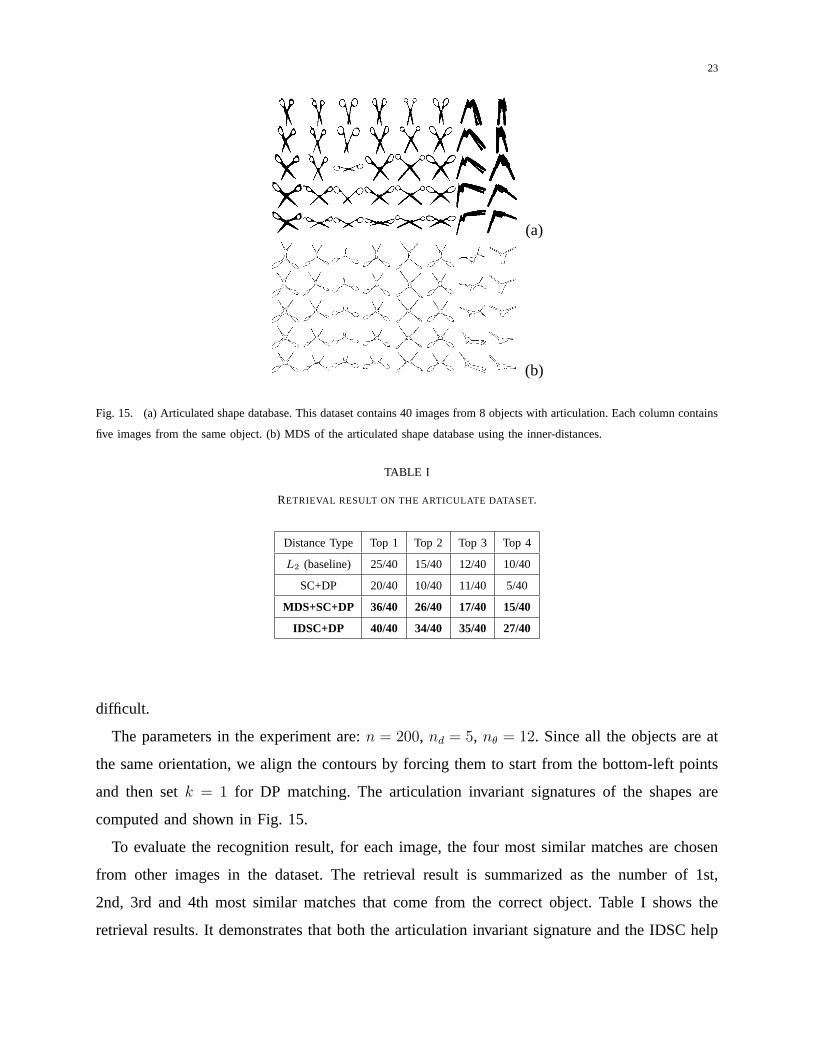
Fig. 15. (a) Articulated shape database. This dataset contains 40 images from 8 objects with articulation. Each column contains
five images from the same object. (b) MDS of the articulated shape database using the inner-distances.
TABLE I
RETRIEVAL RESULT ON THE ARTICULATE DATASET.
Distance Type Top 1 Top 2 Top 3 Top 4
L2 (baseline) 25/40 15/40 12/40 10/40
SC+DP 20/40 10/40 11/40 5/40
MDS+SC+DP 36/40 26/40 17/40 15/40
IDSC+DP 40/40 34/40 35/40 27/40
difficult.
The parameters in the experiment are:n = 200, nd = 5, nθ = 12. Since all the objects are at
the same orientation, we align the contours by forcing them to start from the bottom-left points
and then setk = 1 for DP matching. The articulation invariant signatures of the shapes are
computed and shown in Fig. 15.
To evaluate the recognition result, for each image, the four most similar matches are chosen
from other images in the dataset. The retrieval result is summarized as the number of 1st,
2nd, 3rd and 4th most similar matches that come from the correct object. Table I shows the
retrieval results. It demonstrates that both the articulation invariant signature and the IDSC help
24
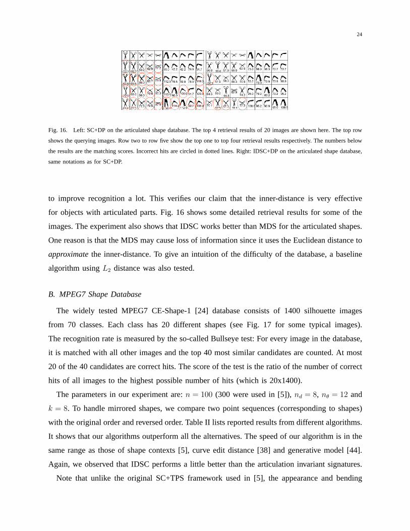
Fig. 16. Left: SC+DP on the articulated shape database. The top 4 retrieval results of 20 images are shown here. The top row
shows the querying images. Row two to row five show the top one to top four retrieval results respectively. The numbers below
the results are the matching scores. Incorrect hits are circled in dotted lines. Right: IDSC+DP on the articulated shape database,
same notations as for SC+DP.
to improve recognition a lot. This verifies our claim that the inner-distance is very effective
for objects with articulated parts. Fig. 16 shows some detailed retrieval results for some of the
images. The experiment also shows that IDSC works better than MDS for the articulated shapes.
One reason is that the MDS may cause loss of information since it uses the Euclidean distance to
approximatethe inner-distance. To give an intuition of the difficulty of the database, a baseline
algorithm usingL2 distance was also tested.
B. MPEG7 Shape Database
The widely tested MPEG7 CE-Shape-1 [24] database consists of 1400 silhouette images
from 70 classes. Each class has 20 different shapes (see Fig. 17 for some typical images).
The recognition rate is measured by the so-called Bullseye test: For every image in the database,
it is matched with all other images and the top 40 most similar candidates are counted. At most
20 of the 40 candidates are correct hits. The score of the test is the ratio of the number of correct
hits of all images to the highest possible number of hits (which is 20x1400).
The parameters in our experiment are:n = 100 (300 were used in [5]),nd = 8, nθ = 12 and
k = 8. To handle mirrored shapes, we compare two point sequences (corresponding to shapes)
with the original order and reversed order. Table II lists reported results from different algorithms.
It shows that our algorithms outperform all the alternatives. The speed of our algorithm is in the
same range as those of shape contexts [5], curve edit distance [38] and generative model [44].
Again, we observed that IDSC performs a little better than the articulation invariant signatures.
Note that unlike the original SC+TPS framework used in [5], the appearance and bending
25
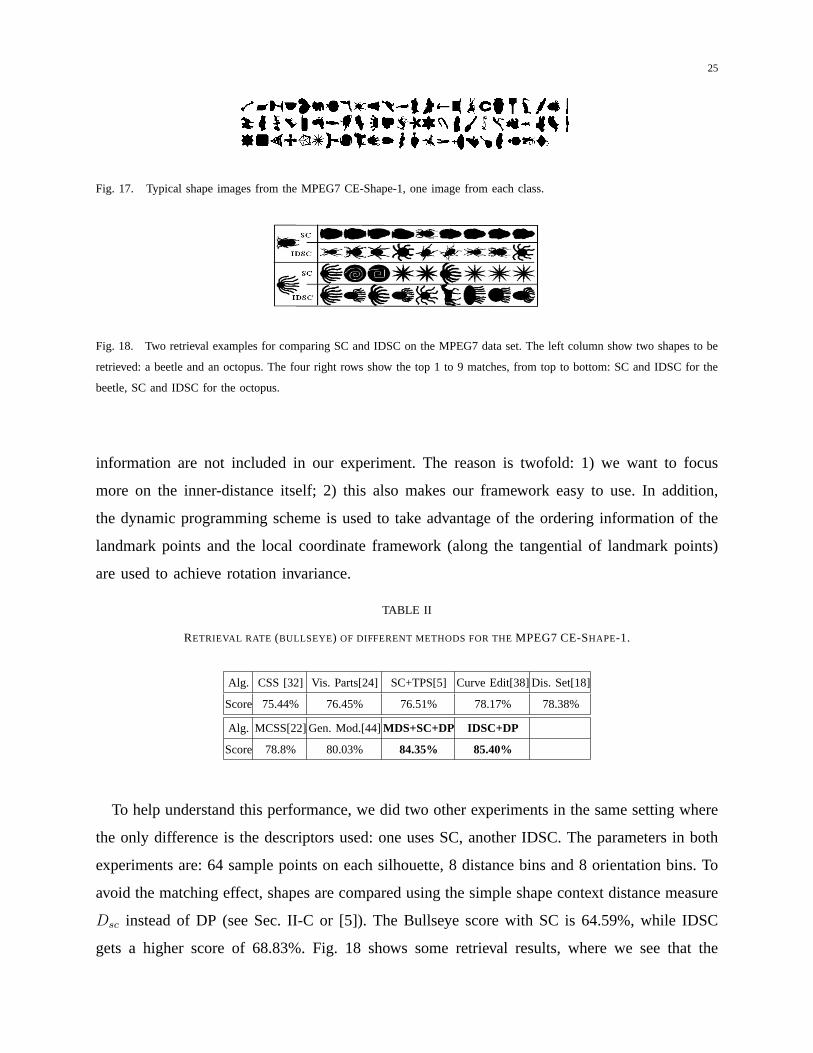
Fig. 17. Typical shape images from the MPEG7 CE-Shape-1, one image from each class.
Fig. 18. Two retrieval examples for comparing SC and IDSC on the MPEG7 data set. The left column show two shapes to be
retrieved: a beetle and an octopus. The four right rows show the top 1 to 9 matches, from top to bottom: SC and IDSC for the
beetle, SC and IDSC for the octopus.
information are not included in our experiment. The reason is twofold: 1) we want to focus
more on the inner-distance itself; 2) this also makes our framework easy to use. In addition,
the dynamic programming scheme is used to take advantage of the ordering information of the
landmark points and the local coordinate framework (along the tangential of landmark points)
are used to achieve rotation invariance.
TABLE II
RETRIEVAL RATE (BULLSEYE) OF DIFFERENT METHODS FOR THEMPEG7 CE-SHAPE-1.
Alg. CSS [32] Vis. Parts[24] SC+TPS[5] Curve Edit[38]Dis. Set[18]
Score 75.44% 76.45% 76.51% 78.17% 78.38%
Alg. MCSS[22]Gen. Mod.[44]MDS+SC+DP IDSC+DP
Score 78.8% 80.03% 84.35% 85.40%
To help understand this performance, we did two other experiments in the same setting where
the only difference is the descriptors used: one uses SC, another IDSC. The parameters in both
experiments are: 64 sample points on each silhouette, 8 distance bins and 8 orientation bins. To
avoid the matching effect, shapes are compared using the simple shape context distance measure
Dsc instead of DP (see Sec. II-C or [5]). The Bullseye score with SC is 64.59%, while IDSC
gets a higher score of 68.83%. Fig. 18 shows some retrieval results, where we see that the
26
IDSC is good for objects with parts while the SC favors global similarities. Examination of
the MPEG7 data set shows that the complexity of shapes are mainly due to the part structures
but not articulations, so the good performance of IDSC shows that the inner-distance is more
effective at capturing part structures.
C. Kimia’s database
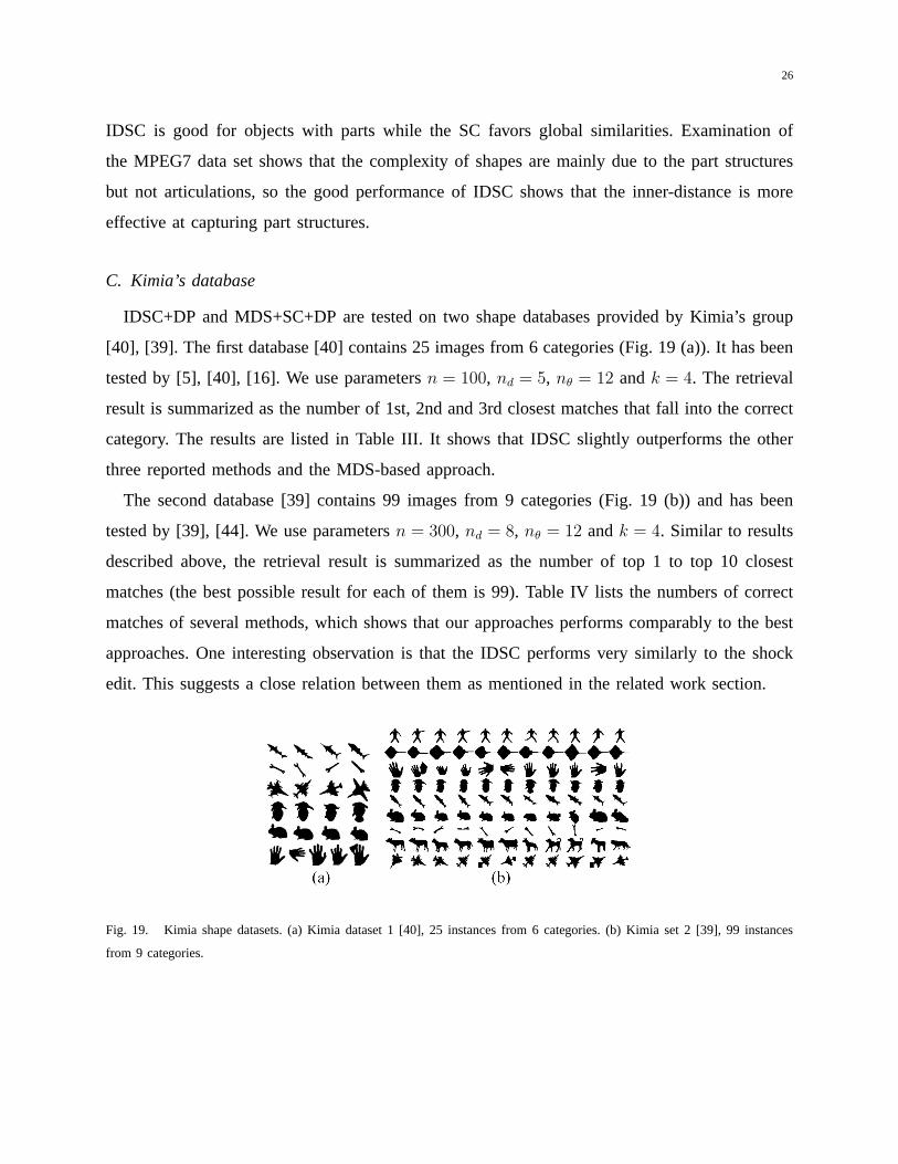
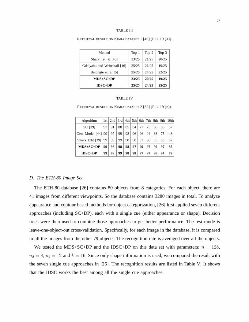
IDSC+DP and MDS+SC+DP are tested on two shape databases provided by Kimia’s group
[40], [39]. The first database [40] contains 25 images from 6 categories (Fig. 19 (a)). It has been
tested by [5], [40], [16]. We use parametersn = 100, nd = 5, nθ = 12 andk = 4. The retrieval
result is summarized as the number of 1st, 2nd and 3rd closest matches that fall into the correct
category. The results are listed in Table III. It shows that IDSC slightly outperforms the other
three reported methods and the MDS-based approach.
The second database [39] contains 99 images from 9 categories (Fig. 19 (b)) and has been
tested by [39], [44]. We use parametersn = 300, nd = 8, nθ = 12 andk = 4. Similar to results
described above, the retrieval result is summarized as the number of top 1 to top 10 closest
matches (the best possible result for each of them is 99). Table IV lists the numbers of correct
matches of several methods, which shows that our approaches performs comparably to the best
approaches. One interesting observation is that the IDSC performs very similarly to the shock
edit. This suggests a close relation between them as mentioned in the related work section.
Fig. 19. Kimia shape datasets. (a) Kimia dataset 1 [40], 25 instances from 6 categories. (b) Kimia set 2 [39], 99 instances
from 9 categories.
27
TABLE III
RETRIEVAL RESULT ON K IMIA DATASET 1 [40] (FIG. 19 (A)).
Method Top 1 Top 2 Top 3
Sharvit et. al [40] 23/25 21/25 20/25
Gdalyahu and Weinshall [16] 25/25 21/25 19/25
Belongie et. al [5] 25/25 24/25 22/25
MDS+SC+DP 23/25 20/25 19/25
IDSC+DP 25/25 24/25 25/25
TABLE IV
RETRIEVAL RESULT ON K IMIA DATASET 2 [39] (FIG. 19 (B)).
Algorithm 1st 2nd 3rd 4th 5th 6th 7th 8th 9th 10th
SC [39] 97 91 88 85 84 77 75 66 56 37
Gen. Model [44]99 97 99 98 96 96 94 83 75 48
Shock Edit [39] 99 99 99 98 98 97 96 95 93 82
MDS+SC+DP 99 98 98 98 97 99 97 96 97 85
IDSC+DP 99 99 99 98 98 97 97 98 94 79
D. The ETH-80 Image Set
The ETH-80 database [26] contains 80 objects from 8 categories. For each object, there are
41 images from different viewpoints. So the database contains 3280 images in total. To analyze
appearance and contour based methods for object categorization, [26] first applied seven different
approaches (including SC+DP), each with a single cue (either appearance or shape). Decision
trees were then used to combine those approaches to get better performance. The test mode is
leave-one-object-out cross-validation. Specifically, for each image in the database, it is compared
to all the images from the other 79 objects. The recognition rate is averaged over all the objects.
We tested the MDS+SC+DP and the IDSC+DP on this data set with parameters:n = 128,
nd = 8, nθ = 12 andk = 16. Since only shape information is used, we compared the result with
the seven single cue approaches in [26]. The recognition results are listed in Table V. It shows
that the IDSC works the best among all the single cue approaches.

28
Fig. 20. ETH-80 image set [26]. This data set contains 80 objects from 8 classes, with 41 images of each
object obtained from different viewpoints. Note: the original images are in color. See http://www.mis.informatik.tu-
darmstadt.de/Research/Projects/categorization/eth80-db.html for detail.
TABLE V
RECOGNITION RATES OF SINGLE CUE APPROACHES ONETH-80 DATABASE [26]. ALL EXPERIMENTS RESULTS ARE FROM
[26] EXCEPT FORMDS+SC+DPAND IDSC+DP.
Alg. Color Hist. DxDy Mag-Lap PCA Masks PCA Gray
Rate 64.85% 79.79% 82.23% 83.41% 82.99%
Alg. SC Greedy SC+DP Decision Tree∗ MDS+SC+DP IDSC+DP
Rate 86.40% 86.40% 93.02% 86.80% 88.11%∗It is a multi-cue method combining all seven previous single-cue methods.
E. Foliage Image Retrieval
In this subsection we will demonstrate the application of the inner-distance on a real and
challenging application, foliage image retrieval. Leaf images are very challenging for retrieval
tasks due to their high between class similarity and large inner class deformations. Furthermore,
occlusion and self-folding often damage leaf shape. In addition, some species have very similar
shape but different texture, which therefore makes the combination of shape and texture desirable.
1) Swedish Leaf Database:The Swedish leaf dataset comes from a leaf classification project
at Linkoping University and the Swedish Museum of Natural History [42]. The dataset contains
isolated leaves from 15 different Swedish tree species, with 75 leaves per species. Fig. 21 shows
some representative silhouette examples. Some preliminary classification work has been done in
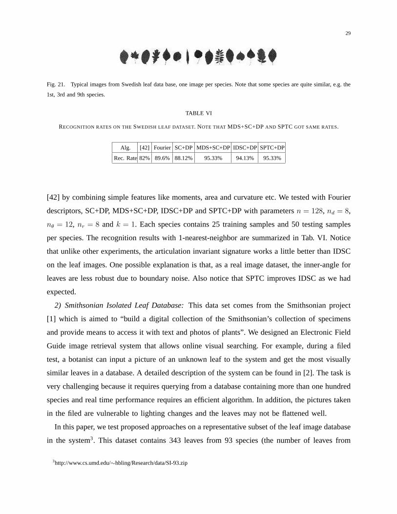
29
Fig. 21. Typical images from Swedish leaf data base, one image per species. Note that some species are quite similar, e.g. the
1st, 3rd and 9th species.
TABLE VI
RECOGNITION RATES ON THESWEDISH LEAF DATASET. NOTE THAT MDS+SC+DPAND SPTCGOT SAME RATES.
Alg. [42] Fourier SC+DP MDS+SC+DPIDSC+DP SPTC+DP
Rec. Rate82% 89.6% 88.12% 95.33% 94.13% 95.33%
[42] by combining simple features like moments, area and curvature etc. We tested with Fourier
descriptors, SC+DP, MDS+SC+DP, IDSC+DP and SPTC+DP with parametersn = 128, nd = 8,
nθ = 12, nr = 8 andk = 1. Each species contains 25 training samples and 50 testing samples
per species. The recognition results with 1-nearest-neighbor are summarized in Tab. VI. Notice
that unlike other experiments, the articulation invariant signature works a little better than IDSC
on the leaf images. One possible explanation is that, as a real image dataset, the inner-angle for
leaves are less robust due to boundary noise. Also notice that SPTC improves IDSC as we had
expected.
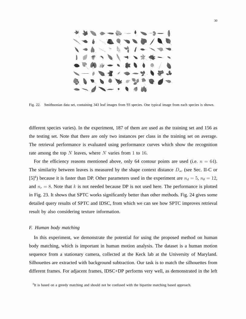
2) Smithsonian Isolated Leaf Database:This data set comes from the Smithsonian project
[1] which is aimed to “build a digital collection of the Smithsonian’s collection of specimens
and provide means to access it with text and photos of plants”. We designed an Electronic Field
Guide image retrieval system that allows online visual searching. For example, during a filed
test, a botanist can input a picture of an unknown leaf to the system and get the most visually
similar leaves in a database. A detailed description of the system can be found in [2]. The task is
very challenging because it requires querying from a database containing more than one hundred
species and real time performance requires an efficient algorithm. In addition, the pictures taken
in the filed are vulnerable to lighting changes and the leaves may not be flattened well.
In this paper, we test proposed approaches on a representative subset of the leaf image database
in the system3. This dataset contains 343 leaves from 93 species (the number of leaves from
3http://www.cs.umd.edu/∼hbling/Research/data/SI-93.zip
30
Fig. 22. Smithsonian data set, containing 343 leaf images from 93 species. One typical image from each species is shown.
different species varies). In the experiment, 187 of them are used as the training set and 156 as
the testing set. Note that there are only two instances per class in the training set on average.
The retrieval performance is evaluated using performance curves which show the recognition
rate among the topN leaves, whereN varies from1 to 16.
For the efficiency reasons mentioned above, only 64 contour points are used (i.e.n = 64).
The similarity between leaves is measured by the shape context distanceDsc (see Sec. II-C or
[5]4) because it is faster than DP. Other parameters used in the experiment arend = 5, nθ = 12,
andnr = 8. Note thatk is not needed because DP is not used here. The performance is plotted
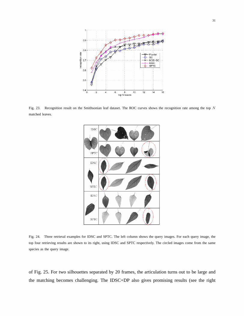
in Fig. 23. It shows that SPTC works significantly better than other methods. Fig. 24 gives some
detailed query results of SPTC and IDSC, from which we can see how SPTC improves retrieval
result by also considering texture information.
F. Human body matching
In this experiment, we demonstrate the potential for using the proposed method on human
body matching, which is important in human motion analysis. The dataset is a human motion
sequence from a stationary camera, collected at the Keck lab at the University of Maryland.
Silhouettes are extracted with background subtraction. Our task is to match the silhouettes from
different frames. For adjacent frames, IDSC+DP performs very well, as demonstrated in the left
4It is based on a greedy matching and should not be confused with the bipartite matching based approach.
31
Fig. 23. Recognition result on the Smithsonian leaf dataset. The ROC curves shows the recognition rate among the topN
matched leaves.
Fig. 24. Three retrieval examples for IDSC and SPTC. The left column shows the query images. For each query image, the
top four retrieving results are shown to its right, using IDSC and SPTC respectively. The circled images come from the same
species as the query image.
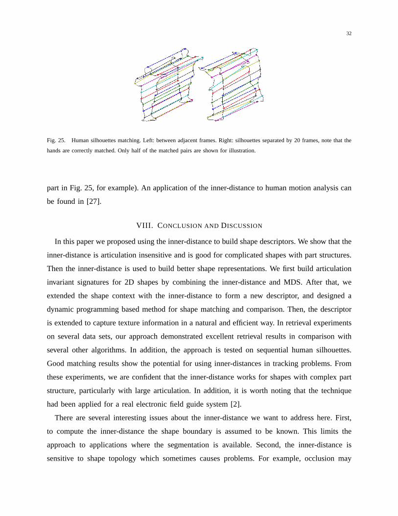
of Fig. 25. For two silhouettes separated by 20 frames, the articulation turns out to be large and
the matching becomes challenging. The IDSC+DP also gives promising results (see the right
32
Fig. 25. Human silhouettes matching. Left: between adjacent frames. Right: silhouettes separated by 20 frames, note that the
hands are correctly matched. Only half of the matched pairs are shown for illustration.
part in Fig. 25, for example). An application of the inner-distance to human motion analysis can
be found in [27].
VIII. C ONCLUSION AND DISCUSSION
In this paper we proposed using the inner-distance to build shape descriptors. We show that the
inner-distance is articulation insensitive and is good for complicated shapes with part structures.
Then the inner-distance is used to build better shape representations. We first build articulation
invariant signatures for 2D shapes by combining the inner-distance and MDS. After that, we
extended the shape context with the inner-distance to form a new descriptor, and designed a
dynamic programming based method for shape matching and comparison. Then, the descriptor
is extended to capture texture information in a natural and efficient way. In retrieval experiments
on several data sets, our approach demonstrated excellent retrieval results in comparison with
several other algorithms. In addition, the approach is tested on sequential human silhouettes.
Good matching results show the potential for using inner-distances in tracking problems. From
these experiments, we are confident that the inner-distance works for shapes with complex part
structure, particularly with large articulation. In addition, it is worth noting that the technique
had been applied for a real electronic field guide system [2].
There are several interesting issues about the inner-distance we want to address here. First,
to compute the inner-distance the shape boundary is assumed to be known. This limits the
approach to applications where the segmentation is available. Second, the inner-distance is
sensitive to shape topology which sometimes causes problems. For example, occlusion may

33
cause the topology of shapes to change. In addition, the inner-distance may not be proper for
shapes involving little part structure and large deformation (no articulation).
ACKNOWLEDGEMENTS
We would like to thank J. W. Kress, R. Russel, N. Bourg, G. Agarwal, P. Belhumeur and
N. Dixit for help with the Smithsonian leaf database; B. Kimia for the Kimia data set, O.
Soderkvist for the Swedish leaf data; Z. Yue and Y. Ran for the Keck sequence. We also thank
the anonymous referees for their helpful comments and suggestions. This work is supported
by NSF (ITR-03258670325867). This research is supported in part by the US-Israel Binational
Science Foundation grant number 2002/254.
REFERENCES
[1] “An Electronic Field Guide: Plant Exploration and Discovery in the 21st Century.”
http://www1.cs.columbia.edu/cvgc/efg/index.php
[2] G. Agarwal, H. Ling, D. Jacobs, S. Shirdhonkar, W. J. Kress, R. Russell, P. Belhumeur, N. Dixit, S. Feiner, D. Mahajan,
K. Sunkavalli, R. Ramamoorthi, and S. White, “First Steps Toward an Electronic Field Guide for Plants,”Taxon, in press.
[3] S. Agarwal, A. Awan, and D. Roth. “Learning to Detect Objects in Images via a Sparse, Part-Based Representation”,IEEE
Trans. Pattern Anal. Mach. Intell., 26(11):1475-1490, 2004.
[4] R. Basri, L. Costa, D. Geiger, and D. Jacobs, “Determining the Similarity of Deformable Shapes”,Vision Research38:2365-
2385, 1998.
[5] S. Belongie, J. Malik and J. Puzicha. “Shape Matching and Object Recognition Using Shape Context,”IEEE Trans. Pattern
Anal. Mach. Intell., 24(24):509-522, 2002.
[6] I. Biederman, “Recognition–by–components: A theory of human image understanding,”Psychological Review, 94(2):115-
147, 1987.
[7] H. Blum. “Biological Shape and Visual Science”.J. Theor. Biol., 38:205-287, 1973.
[8] F. L. Bookstein, “Principal Warps: Thin-Plate-Splines and Decomposition of Deformations,”IEEE Trans. Pattern Anal.
Mach. Intell., 11(6):567-585, 1989.
[9] I. Borg and P. Groenen,Modern Multidimensional Scaling : Theory and Applications, Springer, 1997.
[10] H. Chen, P. Belhumeur and D. W. Jacobs. “In search of Illumination Invariants”,IEEE Conf. on Computer Vision and
Pattern Recognition, I:254-261, 2000.
[11] T. H. Cormen, C. E. Leiserson, R. L. Rivest, and C. Stein.Introduction to Algorithms, MIT Press, 2nd edition, 2001.
[12] A. Elad(Elbaz) and R. Kimmel. “On Bending Invariant Signatures for Surfaces”,IEEE Trans. Pattern Anal. Mach. Intell.,
25(10):1285-1295, 2003.
[13] J. Feldman and M. Singh. “Information along contours and object boundaries”.Psychological Review, 112(1):243-252,
2005.
[14] P. F. Felzenszwalb and D. P. Huttenlocher. “Pictorial Structures for Object Recognition”,Int’l J. of Computer Vision,
61(1):55-79, 2005.

34
[15] R. Fergus, P. Perona and A. Zisserman. “Object Class Recognition by Unsupervised Scale-Invariant Learning”,IEEE Conf.
on Computer Vision and Pattern Recognition, II:264-271, 2003.
[16] Y. Gdalyahu and D. Weinshall. “Flexible Syntactic Matching of Curves and Its Application to Automatic Hierarchical
Classification of Silhouettes”,IEEE Trans. Pattern Anal. Mach. Intell., 21(12):1312-1328, 1999.
[17] L. Gorelick, M. Galun, E. Sharon, R. Basri and A. Brandt, “Shape Representation and Classification Using the Poisson
Equation”, IEEE Conf. on Computer Vision and Pattern Recognition, 61-67, 2004.
[18] C. Grigorescu and N. Petkov. “Distance sets for shape filters and shape recognition”.IEEE Trans. Image Processing,
12(10):1274-1286, 2003.
[19] W. E. L. Grimson, “Object Recognition by Computer: The Role of Geometric Constraints”, MIT Press, Cambridge, MA,
1990.
[20] A. B. Hamza and H. Krim, “Geodesic Object Representation and Recognition”, in I. Nystrom et al. (Eds.):Discrete
Geometry for Computer Imagery, LNCS, 2886:378-387, 2003.
[21] D. D. Hoffman and W. A. Richards, “Parts of recognition,”Cognition, 18:65-96, 1985.
[22] A. C. Jalba, M. H. F. Wilkinson and J. B. T. M. Roerdink. “Shape Representation and Recognition Through Morphological
Curvature Scale Spaces”.IEEE Trans. Image Processing, 15(2):331-341, 2006.
[23] B. B. Kimia, A. R. Tannenbaum, and S. W. Zucker. “Shapes, shocks, and deformations, I: The components of shape and
the reaction-diffusion space”,Int’l J. of Computer Vision, 15(3):189-224, 1995
[24] L. J. Latecki, R. Lakamper, and U. Eckhardt, “Shape Descriptors for Non-rigid Shapes with a Single Closed Contour”,
IEEE Conf. on Computer Vision and Pattern Recognition, I:424-429, 2000.
[25] S. Lazebnik, C. Schmid, and J. Ponce, “A sparse texture representation using affine-invariant regions,”IEEE Trans. Pattern
Anal. Mach. Intell., 27(8):1265-1278, 2005.
[26] B. Leibe and B. Schiele. “Analyzing Appearance and Contour Based Methods for Object Categorization”,IEEE Conf. on
Computer Vision and Pattern Recognition, II:409-415, 2003.
[27] J. Li, S. K. Zhou and Rama Chellappa, “Appearance Modeling Under Geometric Context,”IEEE Int’l Conf. on Computer
Vision, II:1252-1259, 2005.
[28] H. Ling and D. W. Jacobs, “Deformation Invariant Image Matching”,IEEE Int’l Conf. on Computer Vision, II:1466-1473,
2005.
[29] H. Ling and D. W. Jacobs, “Using the Inner-Distance for Classification of Articulated Shapes”,IEEE Conf. on Computer
Vision and Pattern Recognition, II:719-726, 2005.
[30] T. Liu and D. Geiger. “Visual Deconstruction: Recognizing Articulated Objects”,Energy Minimization Methods in Computer
Vision and Pattern Recognition (EMMCVPR), 295-309, 1997.
[31] K. Mikolajczyk and C. Schmid, “A Performance Evaluation of Local Descriptors,”IEEE Trans. Pattern Anal. Mach. Intell.,
27(10):1615-1630, 2005.
[32] F. Mokhtarian, S. Abbasi and J. Kittler. “Efficient and Robust Retrieval by Shape Content through Curvature Scale Space,”
in A. W. M. Smeulders and R. Jain, editors,Image Databases and Multi-Media Search, 51-58, World Scientific, 1997.
[33] G. Mori and J. Malik, “Recognizing Objects in Adversarial Clutter: Breaking a Visual CAPTCHA”,IEEE Conf. on
Computer Vision and Pattern Recognition, I:1063-6919, 2003.
[34] E. N. Mortensen, H. Deng, and L. Shapiro, “A SIFT Descriptor with Global Context”,IEEE Conf. on Computer Vision
and Pattern Recognition, I:184-190, 2005.
[35] R. Osada, T. Funkhouser, B. Chazelle, and D. Dobkin. “Shape Distributions”,ACM Trans. Graphics, 21(4):807-832, 2002.

35
[36] E. G. M. Petrakis, A. Diplaros and E. Milios. “Matching and Retrieval of Distorted and Occluded Shapes Using Dynamic
Programming”,IEEE Trans. Pattern Anal. Mach. Intell., 24(11):1501-1516, 2002.
[37] H. Schneiderman and T. Kanade. “Object Detection Using the Statistics of Parts”,Int’l J. of Computer Vision, 56(3):151-
177, 2004.
[38] T. B. Sebastian, P. N. Klein and B. B. Kimia. “On Aligning Curves”,IEEE Trans. Pattern Anal. Mach. Intell., 25(1):116-
125, 2003.
[39] T. B. Sebastian, P. N. Klein and B. B. Kimia. “Recognition of Shapes by Editing Their Shock Graphs”,IEEE Trans.
Pattern Anal. Mach. Intell., 26(5):550-571, 2004.
[40] D. Sharvit J. Chan, H. Tek, and B. Kimia. “Symmetry-based Indexing of Image Database”,J. Visual Communication and
Image Representation, 9(4):366-380, 1998.
[41] K. Siddiqi, A. Shokoufandeh, S. J. Dickinson and S. W. Zucker. “Shock Graphs and Shape Matching”,Int’l J. of Computer
Vision, 35(1):13-32, 1999.
[42] O. Soderkvist. “Computer Vision Classification of Leaves from Swedish Trees”, Master Thesis, Linkoping Univ. 2001.
[43] A. Thayananthan, B. Stenger, P. H. S. Torr and R. Cipolla, “Shape Context and Chamfer Matching in Cluttered Scenes”,
IEEE Conf. on Computer Vision and Pattern Recognition, I:127-133, 2003.
[44] Z. Tu and A. L. Yuille. “Shape Matching and Recognition-Using Generative Models and Informative Features”,European
Conf. on Computer Vision, 3:195-209, 2004.
[45] R. C. Veltkamp and M. Hagedoorn. “State of the Art in Shape Matching”,Principles of visual information retrieval,
89-119, 2001.
[46] I. Weiss and M. Ray. “Recognizing Articulated Objects Using a Region-Based Invariant Transform”,IEEE Trans. Pattern
Anal. Mach. Intell., 27(10):1660- 1665, 2005.
[47] H. Zhang and J. Malik, “Learning a Discriminative Classifier Using Shape Context Distances”,IEEE Conf. on Computer
Vision and Pattern Recognition, 2003.
[48] L. Zhao and L. S. Davis. “Segmentation and Appearance Model Building from an Image Sequence”,IEEE Int’l Conf. on
Image Processing, 1:321-324, 2005.