1

Source Localization in Reverberant Environments:

Part II - Statistical Analysis

Tony Gustafsson�, Bhaskar D. Rao, and Mohan Trivedi

Abstract

The main di�culty in building robust practical systems for acoustical source localization using microphone arrays, is

the e�ects of room-reverberation. In this paper, a statistical analysis is presented of the in uence of room reverberation

on source localization techniques. Using a statistical reverberation model presented in a companion paper, the Cram�er-

Rao lower bound for time-deley estimation and maximum likelihood estimators are derived. The probability of a large

error is investigated, and also the performance of common time-delay estimation techniques is analyzed. An interesting

outcome of the analysis is that the so-called PHAT time-delay estimator is shown to be optimal among a class of

cross-correlation based time-delay estimators.

SP-EDICS: 2-ROOM

I. Introduction

Several approaches for acoustical source localization and speech acquisition, using microphone arrays, have

appeared in the literature. Microphone arrays have been a promising solution for localization, while at the

same time suppressing interference and noise. In a reverberant environment, the measured signals from a pair

of microphones can be modeled as

x(t) =

Z 1

�1

h(t� �)s(�)d�+ n(t); (1)

where x(t) = [x1(t) x2(t)]T , h(t) = [h1(t) h2(t)]

T , and n(t) = [n1(t) n2(t)]T . Here, hi(t) represents the impulse

response of the acoustical transfer function from the source to the ith microphone, xi(t) is the output of the

ith receiver, s(t) is the unknown source signal, ni(t) is an additive noise term. See for example [13, Chapter

5] for a thorough treatment of the reverberation phenomenon.

This work was performed while T. Gustafsson was visiting University of California San Diego, Department of Electrical and

Computer Engineering, 9500 Gilman Drive Mail Code 0407, La Jolla, CA 92093-0407 USA. email: tgustaf@ece.ucsd.edu. Support

by the Swedish Foundation for International Cooperation in Research and Higher Education, and Telefonaktiebolaget LM Ericsson

is gratefully acknowledged.

B. Rao is with University of California San Diego. email: brao@ece.ucsd.edu. This work was supported by UC DiMi Program

# D97-17.

M. Trivedi is with University of California San Diego. email: trivedi@ece.ucsd.edu.

2

Most existing techniques for source localization, cf. [4], [2], [15], [17], are however based on the simpler

model

x1(t) = s(t) + n1(t)

x2(t) = s(t� �0) + n2(t);(2)

where �0 denotes the time-delay. This simple propagation model is not very realistic in practical environments.

Among the few analyses available on the in uence of reverberation on the estimate of �0, we mention [5], [9].

In [9], Ianniello studied the case with one source and two or three resolvable propagation paths. The e�ects

of multi-path were then analyzed by computing a lower bound on the probability of large error estimates.

However, since room reverberation consists of the superposition of a large number of echoes from di�erent

directions with di�erent magnitudes, the results in [9] are limited in analyzing the e�ects of reverberation. In

[5], Champagne et al. presented results using the image method for simulating the reverberant channel h(t).

An interesting result of [5], was that the authors proposed a Cram�er-Rao lower Bound (CRB) for the variance

of the estimated time-delay, when reverberation is present. The introduced CRB showed good agreement with

Monte-Carlo simulations. There was however no analytical motivation of why the introduced CRB should be

relevant. Nevertheless, the numerical study in [5] clearly demonstrated the adverse e�ects of reverberation.

The purpose of the present paper is analyze of the problem of acoustic source localization in a reverberant

environment. The statistical analysis is based on a model proposed in a companion paper [7]. Using the model

of [7], several interesting results are derived. Among others, we will derive the CRB for estimation of �0.

II. Review of Single-path Propagation Time-delay Estimation (TDE)

The Generalized Cross Correlation (GCC) [12] method is probably the most popular method for estimating

time-delays. Its popularity is due to high accuracy, and low computational complexity which is achieved by

Fast Fourier Transform (FFT) implementations. In the GCC method, the estimated time-delay is obtained

as

� = argmax�

RGCC(�); (3)

where

RGCC(�)4=

Z 1

�1

jG(!)j2P12(!)ej!� ; (4)

and P12(!)4= X2(!)X

�1 (!) denotes the estimated cross-power spectrum. Here, Xi(!) denotes the Fourier

transform of xi(t) over a �nite interval 0 � t � T , the superscript (�)� denotes complex conjugate, and

jG(!)j2 is a weighting function. Under certain conditions, the GCC method is the Maximum Likelihood (ML)

estimator of �0 [12]. The CRB (assuming s(t), n1(t) and n2(t) to be zero-mean, mutually uncorrelated wide-

sense stationary Gaussian random processes with power spectra Pss(!), Pn1n1(!) and Pn2n2(!) respectively)

3

is further known to equal

CRBsp(�0) =

�2T

Z 1

0

SNR(!)2

1 + 2SNR(!)!2d!

��1(5)

where we for notational simplicity assumed that Pn1n1(!) = Pn2n2(!). The subscript (�)sp indicates that the

CRB is valid for the single-path propagation model (2). In the CRB expression (5), we also introduced the

signal to noise ratio (SNR)

SNR(!) =Pss(!)

Pnini(!): (6)

>From the above brief review we may conclude that TDE under single-path propagation is a well-understood

problem. Much less is known about TDE when reverberation is present. Several authors have for example

observed that the PHAse Transform (PHAT) method is more robust than other GCC methods in reverberant

environments, cf. [3], [10], [16]. PHAT is also a member of the GCC class of algorithms, and is obtained with

the following choice of weighting:

jGPHAT (!)j2 =

1���P12(!)��� : (7)

An analytical motivation of why PHAT is more robust than ML is however not available in the literature.

III. Brief Review of the Reverberation Model

We next brie y review the properties of the model introduced in [7]. Throughout the paper it will be

assumed that only a sampled version of x(t) is available, i.e. fx(nTs)gN�1n=0 where Ts is the sampling interval.

The source signal s(t) is assumed band-limited, i.e. its power is zero outside the interval [fl; fu] Hz. We

further assume that frequency domain data are obtained from the DFT of the sequence x(nTs), which implies

a frequency domain sampling !k = 2�Fs=N , k = 0; 1; � � � ; N � 1, where Fs = 1=Ts. We will further assume

that the considered array of microphones consists of a uniform linear array with M microphones. It is then

assumed that the DFT of x(nTs) obeys the model

X(!k) = (A(!k; �0) +R(!k;�))S(!k); k = kl; � � � ; ku; (8)

where

kl = round

�NflFs

�(9)

ku = round

�NfuFs

�(10)

A(!k; �0) =h1 e�j!k�0 � � � e�j!k�0(M�1)

iT: (11)

The M -dimensional vector R(!k;�) is assumed to be zero-mean, circularily symmetric Gaussian, and to have

a covariance matrix E��R(!;�)R(!;�)H

= �2IM . Here (�)H denotes complex conjugate transpose, E�f�g

4

denotes the expectation operator with respect to all source/microphone positions, and

�2 =16�r2�2

A(1� �2): (12)

In the above relationship, r denotes the distance from the source to the array, � denotes the re ection

coe�cient of the re ecting surfaces of the room in question, A denotes the total wall area, and S(�) denotes

the DFT of the source signal.

As discussed in [7], R(!k;�) and R(!l;�) are in general correlated, unless the frequency separation j!k�!lj

is large. We will discuss this issue in more detal later on.

IV. The Cram�er-Rao Lower Bound for TDE

We begin our statistical investigation by deriving the Cram�er-Rao lower Bound (CRB) for estimation of �0,

based on the model (8). It is not obvious what kind of assumptions we should impose on S(!). Two options

are immediate:

S1: Suppose that fS(!k)gkuk=kl

are unknown but deterministic parameters.

S2: Suppose that fS(!k)gkuk=kl

is a sequence of independent zero-mean Gaussian random variables with vari-

ances Pss(!k).

Remark 1: Note, if s(t) is a wide-sense stationary random processes, the Gaussianity, mutual independence,

and variance of S(!k) assumed in S2, hold asymptotically (i.e. as N !1) under mild assumptions. See for

example [11, Chapter 15].

The outcome of the statistical analysis certainly depends on how S(!k) is modeled. In the narrowband

sensor array processing case, the corresponding CRB's are commonly referred to as deterministic/conditional

and stochastic/unconditional CRB's (see for example the discussion in [19]). In the sensor array processing

literature, it is well known that the CRB corresponding to the deterministic case usually is too optimistic and

hence unreachable. In the present scenario, the deterministic CRB would in general depend on the correlation

length �(T60) of R(!;�) (cf. the de�nition in [7]). Based on these observations, we have chosen to omit the

deterministic case in the present investigation.

Consider next the stochastic case S2. Also in this case we face some technical problems. The reason for

this is the assumed Gaussianity of R(!;�) and S(!), leaving the distribution of their product undetermined.

However, in the following we ignore this fact, and heuristically assume that also X(!k) is Gaussian.

Due to the assumed whiteness of S(!k) (i.e. S2), X(!k1) and X(!k2) are independent. This observation

holds irrespective of the value of the coherence bandwidth �(T60). To see this, study the expected value of

the product of two arbitrary elements X(!k) and X(!l) (k 6= l):

E�;S

n(A(!k)S(!k) +R(!k;�)S(!k)) (A(!l)S(!l) +R(!l;�)S(!l))

Ho

= ES fS(!k)S(!l)�g| {z }

=0

E�

n(A(!k) +R(!k;�)) (A(!l) +R(!l;�))

Ho= 0:

(13)

5

The result follows from the whiteness of S(!k) and the mutual independence of R(!;�) and S(!). For the

above result to hold true, the expectation operator must be de�ned as the ensemble average over all signal

realizations, and over all source/microphone positions, denoted as E�;Sf�g. Note that if S(!k1) and S(!k2)

were correlated, or if we used the deterministic setting S1, the relationship (13) would not be true, and the

CRB computation would become more complicated.

Proposition 1: Suppose that fX(!k)gkuk=kl

is a sequence of independent zero-mean Gaussian random vari-

ables with

E�;S�X(!k)X(!k)

H

= Pss(!k)��2IM +A(!k; �0)A(!k; �0)

H�

(14)

E�;S�X(!k)X(!k)

T

= 0; (15)

where Pss(!k) > 0. Then, any unbiased estimator � of the true time-delay �0 satis�es

E�;S

n(� � �0)

2o� CRBrev(�0;M) =

�4Pkuk=kl

Tr fPkDkPkDkg(16)

where subscript \rev" indicates CRB for the reverberation model,

Dk4= A(!k; �0)D

H(!k; �0) +D(!k; �0)AH(!k; �0) (17)

Pk4= IM �

A(!k; �0)AH(!k; �0)

�2 +M(18)

D(!k; �0)4=

@A(!k; �)

@�; (19)

where the right hand side of (19) is evaluated at � = �0.

Proof: See Appendix A.

To gain some insight into the above results, we next evaluate the CRB for the interesting case whenM = 2:

Corollary 1: Under the same assumptions as in Proposition 1, but for the special case M = 2, expression

(16) simpli�es to

CRBrev(�0;M = 2) =

0@2 SRR2

1 + 2SRR

kuXk=kl

!2k

1A�1 (20)

where the Signal to Reverberation Ratio (SRR) is de�ned as

SRR4=

1

�2=A(1� �2)

16�r2�2: (21)

Proof: Straightforward calculations which are omitted.

It is interesting to note the similarity between (20) and the CRB expression for single-path time-delay

estimation in additive noise (5). The expression (20) does however not contain the power spectrum of the

source signal, which is an important distinction.

6

Remark 2: Next we would like to comment on how to include the e�ects of additive measurement noise in

the above CRB expressions. Assuming that the additive noise ni(t) is zero-mean, white, Gaussian, and with

variance �2, the CRB expression for the case with additive measurement noise present reads as

]CRBrev(�0;M = 2) =

0@2 kuX

k=kl

SNRR(!k)2

1 + 2SNRR(!k)!2k

1A�1 (22)

where the signal to noise and reverberation ratio (SNRR) is de�ned as

SNRR(!) =Pss(!)

14�r2

Pss(!)4�2

A(1��2)+ �2

: (23)

Note that Pss(!) now appears in the CRB, in contrast to (20).

A promising approach to analyze the accuracy of � (as de�ned in equation (3)) was recently proposed in [5].

It was suggested that the single-path CRB (5) is valid also in reverberant environments, with the important

modi�cation that SNR(!) is modi�ed to account for reverberation. The \equivalent SNR" suggested in [5]

reads as

(SNReq(!))i =jHi(!; 0)j2Pss(!)

Pnini(!) + jHi(!;�)�Hi(!; 0)j2Pss(!); (24)

where Hi(!; 0) denotes the transfer functio from the source to the ith microphone in case of no reverberation,

and Hi(!;�) denotes the same transfer function with reverberation included. We note that the SNRR in (23)

corresponds to the average value of SNReq (24), assuming that the quantity (Hi(!;�)�Hi(!; 0)) corresponds

to di�use sound. We have however, in contrast to [5], derived CRBrev(�0) under precise modeling assumptions.

V. Analysis of GCC Techniques

A. The Probability of an Anomalous Estimate

Knowledge of CRBrev(�0) for a particular room con�guration is certainly an important factor to consider.

However, the derived CRB is rather local in the sense that it is reachable only for large SRR. In practical

applications, the limiting factor of the performance is rather the fact that GCC-based localization methods

su�er from outliers, simply because the \wrong peak" of the GCC function RGCC(�) is selected. It is therefore

of great interest to analyze the probability of an anomalous estimate, or in other words, the probability of

selecting the wrong peak of RGCC(�). For the case with single-path propagation and additive measurement

noise, Ianniello analyzed this probability in a classical paper [8]. The purpose of the following section is then

to extend Ianniello's analysis to include reverberation.

In addition to the general assumptions introduced in Section III, we introduce the following assumptions:

E1: Assume that the sampled source signal s(nTs) is a zero mean white ergodic random process:

ES fs(nTs)g = 0 (25)

ES fs(nTs)s((n+ l)Ts)g = Rss�l; (26)

7

where �l denotes Kronecker's delta function.

E2: Assume that m� ~N � N , where ~N4= Fs=�(T60).

The basic idea of the analysis technique is as follows. For a given realization h(t;�), the conditional cross-

correlation between x1(t) and x2(t) equals

ESfx1(t)x2(t� �)j�g = h1(� ;�) � Rss(�) � h2(�� ;�); (27)

where � denotes convolution, and Rss(�) denotes the auto-correlation function of s(t). Hence, even if s(t)

is ergodic and if N ! 1, it cannot be expected that the maximum of ESfx1(t)x2(t � �)j�g appears in the

vicinity of �0. For N large (as dictated by Assumption E2), the analysis should focus on the behavior of the

random variable ESfx1(t)x2(t� �)j�g. The measurement time N will hence not appear in our analysis.

Consider now the GCC function, which is computed using x(nTs) to produce the sequence fRGCC(nTs)g

where n = ��m;��m + 1; � � � ; �m and �m = d=(cTs). Here, �m denotes the maximum relative time-delay. If

the sequence fRGCC(nTs)g consists of independent random variables, a reasonable de�nition of an anomalous

event is the following:

E4=hRGCC(nTs) > RGCC(n0Ts) for at least one [��m; �m] 3 n 6= n0

i(28)

where n0 corresponds to the true time-delay (to simplify the presentation we assume that n0 = �0=Ts and �m

are integers). The above de�nition of the anomalous event E is essentially taken from [8]. In [8], the anomalous

event E was de�ned using the correlation length of s(t). More precisely, if Tc denotes the correlation length

of s(t), E was de�ned by sampling RGCC(�) with sampling interval Tc.

If we next denote the number of available samples of the GCC function as m = 2�m + 1, the probability of

an outlier can be computed from (see [8])

Prob[Outlier] ' Prob[E ] = 1�

Z 1

�1

p(z0)

�Z z0

�1

p(zn)dzn

�m�1dz0: (29)

Here we introduced the following notations:

� z04= RGCC(n0Ts), i.e. the value of the GCC function for the true time-delay.

� zn4= RGCC(nTs), for n 6= n0.

� p(z0): the probability density function (PDF) of z0.

� p(zn): the PDF of zn for n 6= n0.

Note, the expression (29) for the outlier probability only makes sense if the sequence RGCC(nTs) consists of

mutually independent random variables. The strategy for analyzing Prob[Outlier] should then be clear:

1. Determine under which conditions the sequence fRGCC(nTs)g�mn=��m consists of mutually independent ran-

dom variables.

2. Find the PDF's p(z0) and p(zn).

8

3. Evaluate the integral (29).

We then have the following interesting result:

Proposition 2: Under the general assumptions introduced in Section III and under assumptions E1-E2, the

sequence fRGCC(nTs)g�mn=��m consists of mutually independent random variables with the following distribu-

tions (assuming that jG(!)j2 = 1):

RGCC(n0Ts) 2 N

�Rss;

R2ss

~N

�2

SRR+

1

SRR2

��(30)

RGCC(nTs) 2 N

�0;R2ss

~N

�2

SRR+

1

SRR2

��: (31)

Proof: See Appendix B

To compute the probability of an outlier, it only remains to compute the integral (29) using the results in

Proposition 2. This integral has to be implemented using numerical integration. A couple of remarks are in

place:

Remark 3: Since ~N is proportional to T60, one may erroneously think that the variance of RGCC(nTs)

decreases as the reverberation time increases. This is however not correct since 1=SRR increases at a faster

rate than ~N , as T60 increases.

Remark 4: Previously we assumed that s(t) is white. In a practical setup with s(t) representing speech, the

whiteness assumption is typically violated. To avoid these di�culties, Ianniello used the correlation length of

s(t) in his de�nition of the event E . However, we conjecture that Proposition 2 is relevant also for colored

signals, assuming that we apply a GCC method (such as PHAT) that employs pre-whitening.

Remark 5: In the numerical experiments, we will study source signals which are spectrally at within an

interval [fl; fu]. A simple approach to modify the variance expressions in Proposition (2), to accommodate

for the band-pass characteristics of s(t), is to replace ~N with 2 ~N (fu� fl)=Fs. This modi�cation is applied in

the numerical examples.

With the above results on the probability of selecting the wrong peak of the GCC function, we can also

predict how accurately it is possible to estimate the time-delay in a reverberant environment. For that

purpose, assume that the variance of the GCC estimate � equals CRBrev(�0) in cases where the correct peak

is selected. Furthermore, in cases where the wrong peak is selected, we assume that � is uniformly distributed

in the interval [�d=c; d=c]. Then the variance of the estimated time-delay � approximately can be found from

the following expression:

E�;S�(� � �0)

2' (1� Prob[E ]) CRBrevs(�0) + Prob[E ]

d2

3c2: (32)

The variance expression (32) is then a more realistic (and more pessimistic!) bound than CRBrev(�0).

9

B. Variance of �

As previously mentioned, several authors have noticed that PHAT performs better than other GCC methods

in reverberant conditions. The purpose of the following section is to provide an analytical motivation of this

empirical observation. As in the previous section, we will focus on the behaviour of the random variable

ESfx1(t)x2(t � �)j�g. Hence, it is assumed that N is large. As in the proof of Proposition 2, it is assumed

that the frequency axis is sampled according to the coherence bandwidth of R(!;�) (cf. equations (104) and

(105)).

For any choice of the GCC weighting jG(!)j2, the estimated time-delay can approximately be written as1

� = argmin�

V (�); (33)

where

V (�)4= �

8<:

kuXk=kl

jG(�k)j2�P12(�k;�)e

j�k� + P12(�k;�)�e�j�k�

�9=; (34)

P12(�k;�) = Pss(�k)

0B@e�j�k�0 +R2(�k;�) +R�1(�k;�)e

�j�k�0| {z }�(�k)

+R2(�k;�)R�1(�k;�)| {z }

~�(�k)

1CA : (35)

Furthermore,

�k =2�Fs~N

; k = �~N

2; � � � ;

~N

2� 1 (36)

~N =Fs

�(T60): (37)

In the above, P12(�k;�) denotes the Fourier-transform of ESfx1(t)x2(t � �)j�g. The basic idea in the

following is to analyze the accuracy of � (de�ned as in (33)) for small levels of the reverberation power �2. To

perform the analysis, we assume that � is consistent in the sense that � ! �0 as � ! 0. As is well-known from

the literature on sensor array signal processing, a su�cient condition for guaranteeing consistency, is that

d �c

2fl; (38)

where c denotes the propagation speed. Since � minimizes V (�), we have V 0(� ) = 0, where V 0(� ) denotes the

gradient of V (�) evaluated at � . For high SRR, a �rst order Taylor expansion yields

0 = V 0(�0) + V 00(�0) (� � �0) + op�jV 0(�0)j

�; (39)

where V 00(�0) denotes the Hessian, and op(�) is order in probability. It now follows that

� � �0 = �1

ZV 0(�0) + op

�jV 0(�0)j

�: (40)

1This approximation assumes that Pss(!) is a \smooth" function of !, in relation to the coherence-bandwidth �(T60).

10

where

Z4= lim

�!0V 00(�0): (41)

For high SRR, and N large, we �nd that the mean square error of the estimation error is given by

E�

n(� � �0)

2o= �2

K

Z2+ o(�2); (42)

where

K4= lim

�!0

1

�2E�

n�V 0(�0)

�2o: (43)

Note then that

E� f�(�k)�(�k)�g = 2�2 (44)

E� f~�(�k)~�(�k)�g = �4 (45)

E� f�(�k)~�(�k)�g = 0: (46)

Since we in equation (42) neglect all terms that are of order o(�2), P12(�k;�) is approximated as

P12(�k;�) ' Pss(�k)�e�j�k�0 + �(�k)

�(47)

Next, we compute the gradient and Hessian matrices as

V 0(�) =@

@�V (�) = �

1

2

kuXk=kl

jG(�k)j2�P12(�k;�)(j�k)e

j�k� + P12(�k;�)�(�j�k)e

�j�k��

(48)

V 00(�) =@

@�V 0(�) =

1

2

kuXk=kl

jG(�k)j2�2k

�P12(�k;�)e

j�k� + P12(�k;�)�e�j�k�

�: (49)

Since P12(�k;�)! Pss(�k)e�j�k�0 as � ! 0, we �nd that the Hessian, evaluated at � = �0, can be written as

Z4= lim

�!0V 00(�0) =

kuXk=kl

jG(�k)j2�2kPss(�k): (50)

Consider next the computation of K. Applying the approximation (47), we obtain

V 0(�0) ' �1

2

kuXk=kl

jG(�k)j2(j�k)Pss(�k)

n(e�j�k�0 + �(�k))e

j�k�0 � (ej�k�0 + �(�k)�)e�j�k�0

o

= �1

2

kuXk=kl

jG(�k)j2(j�k)Pss(�k)

n�(�k)e

j�k�0 � �(�k)�e�j�k�0

o;

(51)

where f�(�k)g is a sequence of circularly symmetric zero-mean independent Gaussian random variables. Hence,

11

using the assumption that �(�k) and �(�l) are independent for �k 6= �l, it follows that

K = lim�!0

1

�2E�

8<:

kuXk=kl

1

4jG(�k)j

4�2kPss(�k)2n�(�k)e

j�k�0 � �(�k)�e�j�k�0

on�(�k)e

j�k�0 � �(�k)�e�j�k�0

o�o

= lim�!0

1

�2

0@ kuXkl=1

1

4jG(�k)j

4�2kPss(�k)22�2

1A =

1

2

klXk=kl

jG(�k)j4�2kPss(�k)

2;

(52)

and the derivation of E�

n(� � �0)

2ois complete.

The mean square error (42) clearly depends on how the weighting sequence jG(�k)j2 is chosen. An interesting

question is how jG(�k)j2 should be chosen for lowest possible error variance. The optimal choice of jG(�k)j

2

is provided in the following result:

Proposition 3: The lowest possible error variance E�

n(� � �0)

2o' �2 K

Z2 is obtained if

jGopt(�k)j2 =

1

Pss(�k): (53)

Proof: De�ne the following matrices

�T 4

=h�klpPss(�kl) � � � �ku

pPss(�ku)

i(54)

G4= diag

njG(�kl)j

2 ; � � � ; jG(�ku)j2o

(55)

�4= diag fPss(�kl); � � � ; Pss(�kl)g : (56)

Then it is easy to see that

K

Z2=

1

2

��

TG�

��1�

TG�G�

��

TG�

��1: (57)

Assuming that Pss(�k) > 0 for k = kl; � � � ; ku, it follows from well-known matrix optimization results (see

for example [14, Appendix II.2]) that the best possible weightings are given by Gopt = ��1, and the proof is

complete.

In general the quantity Pss(�k) is unknown. However, note that���E�;S nP12(�k)o��� = ���Pss(�k)e�j�k�0��� = Pss(�k): (58)

Hence, a natural estimate of Pss(�k) is Pss(�k) =���P12(�k)���. It is then interesting to see that the resulting

estimator corresponds to the PHAT time-delay estimator, compare with equation (7). The above calculations

have shown that PHAT in reverberant environments should be considered as the prime choice among the

GCC estimators, which agrees well with previous empirical observations cf. [3], [10], [16].

VI. ML Estimation of �0

The previous section dealt with the problem of analyzing the accuracy of TDE in reverberant environments.

Although we showed that PHAT may be considered as the best GCC-estimator, is of interest to study the

12

actual ML estimator of �0. It should also be noted that PHAT is applicable only to the case with M = 2

microphones, whereas the ML estimator can include measurements fromM � 2 microphones. In the following,

we study two di�erent approaches to �nding the ML estimate of �0. These two approaches are obtained by

using slightly di�erent models for X(!k).

A. \Stochastic" ML

In the �rst case, we assume that the sequence fX(!kgkuk=kl

consists of independent and Gaussian random

variables:

X(!k) 2 N�0; Pss(!k)

��2IM +A(!k; �0)A(!k; �0)

H��: (59)

Concentrating the likelihood function with respect to fPss(!k)gkuk=kl

, straighforward caluclations show that

the ML estimator of �0 and �2 is obtained by minimizing the following criterion function:

VSML(�; �2) =

kuXk=kl

M log

�X(!k)

H

�IM �

A(!k; �)A(!k; �)H

�2 +M

�X(!k)

�

+ (ku � kl + 1)

�1 +

M

�2

�:

(60)

The criterion-function VSML(�) clearly depends on both �2 and � . Unfortunately VSML(�) cannot be con-

centrated with respect to �2, which leads to a prohibitively high computational complexity. Therefore, we

consider the resulting estimator to be of theoretical interest only.

B. Approximate ML

To �nd an estimator that is more attractive from a computational point of view, we next propose an

Approximative ML (AML) estimator. To arrive at the desired solution, it is assumed that the sequence

fX(!k)gkuk=kl

consists of independent and Gaussian random variables with the following distribution:

X(!k) 2 N�A(!k)S(!k); �

2kIM

�: (61)

Hence, it is now assumed that fS(!k)gkuk=kl

consists of unknown but deterministic parameters. We further

ignore the fact that the variance of X(!k) is proportional to jS(!k)j2. Instead, we allow the parameters �2k

to be frequency dependent. Note, the introduced model clearly violates the assumed frequency correlation of

R(!;�), since X(!k1) and X(!k2) are assumed independent, while assuming that S(!k) is deterministic. We

however ignore this fact in the derivation of the AML-estimator.

Concentrating the resulting likelihood function with respect to all nuisance parameters, the following crite-

rion function is obtained:

VAML(�) =kuXk=kl

log

� �?k (�)X(!k)

2� ; (62)

13

where�?k (�) denotes the projection matrix onto the orthogonal complement of the space spanned byA(!k; �):

�?k (�)

4= IM �

A(!k; �)A(!k; �)H

M: (63)

The time-delay �0 is estimated by minimizing VAML(�) with respect to � :

� = argmin�

VAML(�): (64)

The main advantage with the AML approach, is that VAML(�) is a function of � only, which is an important

observation considering real-time implementations. The criterion function VAML(�) is unfortunately non-

linear in � . To speed up the calculations, we only compute VAML(�) on the grid � = nTs for lag-values

jnj = 0; 1; � � � ; �m. Finally, quadratic interpolation is used to re�ne the estimate so obtained [8].

Remark 6: In the literature on direction �nding for wide-band signals, estimators quite similar to the AML

estimator have appeared. For example, in [6] the deterministic ML estimator of �0 was derived assuming �2k

to be constant over the frequency band of interest. The resulting cost-function is identical to (62), with the

distinction that logf�g is missing.

VII. A Robust Procedure for Source Localization

The purpose of this section is to propose a new source localization method. The key observation is that

the reverberation model strongly (via the factor �(r)2) depends on the distance between the speaker and

the microphones. Although not included in the model, there is in practice also a strong dependence on the

orientation of the speaker. Given a number of microphones distributed over the spatial region of interest, it

is clear that time-delays estimated by microphones close to the speaker should be favored in the localization

procedure. We should also favor the microphones (if any!) which the speaker are facing. However, if only

audio information is available, it is far from obvious how to decide which of the estimated time-delays that

should be trusted the most. In the following, a novel procedure for weighting of the estimated time-delays will

be proposed.

Suppose that P di�erent microphone pairs are distributed over the spatial region. The estimated time-delays

are collected in the vector

�4=h�1; � � � ; �P

iT: (65)

Next we wish to estimate the unknown location of the source, denoted rs. Given � , several di�erent approaches

to solve this problem have been proposed, see for example [2], [17], [18]. Here we focus on a weighted least

squares approach: de�ne the estimated source location as

rs = argminrs

(� � � (rs))TW (� � � (rs)) ; (66)

14

where the vector � (rs) contains the theoretical time-delays as a function of rs, and W is a positive de�nite

weighting matrix. In the following we will consider the case whenW is diagonal, i.e. W = diagfw1; � � � ; wP g.

Hence, we implicitly assume that the estimated time-delays are statistically independent. Considering (66),

it is intuitively clear that the elements of W should be inversely proportional to the variance of � . Such a

weighting strategy would be optimal if � is Gaussian.

The key problem is how the variance of � can be derived from the available data. The variance of � seems

quite di�cult to estimate, and we resort to approximative procedures. For that purpose, recall Proposition 2,

which stated that RGCC(nTs), for n 6= n0, is Gaussian with zero-mean and variance proportional to 2�2+�4.

Note next that CRBrev(�0;M = 2) (20) is proportional to (2�2 + �4). Hence,

Var(R(nTs)) � CRB(�0;M = 2); (67)

where � denotes \proportional to". The basic idea is hence to estimate the quantity Var(R(nTs)), and use

this estimate instead of the unknown variance of � .

The proposed algorithm for robust source localization reads as follows:

1. Compute the GCC function for each microphone pair, i.e. evaluate fRpGCC(nTs)g

�mn=��m for p = 1; � � � ; P

2. Compute the pth time-delay as

np = argmaxn

RpGCC(nTs): (68)

3. Compute the pth weight as

wp =1P

n6=np

�RpGCC(nTs)

�2 ; (69)

where the summation is restricted to lag-values in the interval [��m; �m].

4. Minimize (66) with respect to rs, using W = diagfw1; � � � ; wP g.

In practice we have noted that a slight modi�cation of wp is bene�cial. The observation we have made, is that

realizations of RpGCC(nTs) where the di�erence between the largest and the second largest value of Rp

GCC(nTs)

is small, should have a smaller weight. Hence, in our experiments, the following value of wp has been applied:

wp =�pP

n6=np

�RpGCC(nTs)

�2 ; (70)

where �p denotes the di�erence between the largest and the second largest value of RpGCC(nTs).

Before we proceed to the numerical examples, it should be noted that Proposition 2 holds under rather

restrictive assumptions (such as s(nTs) being white). Hence, we believe that the proposed procedure for

robust source localization should be used together with PHAT. This since the PHAT weighting achieves a

kind of pre-�ltering, which should make it more likely that the conditions of Proposition 2 are ful�lled.

15

VIII. Numerical Examples

A. TDE Accuracy

In the following, the sampled source signal s(nTs) is generated by �ltering of a zero-mean white Gaussian

noise sequence with unit variance through a 6th order band-pass Butterworth �lter. The cut-o� frequencies

of the Butterworth �lter were chosen as fl = 300 Hz and �fu = 3500 Hz, respectively. The signal bandwidth

then roughly corresponds to the frequency band of human speech. The sampled source signal is subsequently

convolved with the simulated room response h(nTs), which results in the sampled microphone signal x(nTs).

To generate independent realizations of R(!;�), we apply the image method [1], and the procedure described

in [7].

In the following, three di�erent time-delay estimators are studied:

� CC: Ordinary cross-correlation. That is, choose the GCC weighting as jG(!)j2 = 1.

� PHAT.

� AML.

All algorithms are evaluated on a grid jnjTs = 0; 1; � � � ; �m. To re�ne the estimated time-delay, quadratic

interpolation is applied as in [8]. In all simulations, we further use N = 2048 samples to estimate the

time-delay, and for each value of the reverberation time T60, 100 Monte-Carlo simulations are performed. In

the derivation of the outlier probability, we used the coherence band-width �(T60) to construct uncorrelated

snapshots of R(!;�). Furthermore, in [7], two reasonable de�nitions were introduced: �(T60) = 2=T60 and

�(T60) = 7=T60. The outcome of the theoretical outlier probability certainly depends on which de�nition

we chose. Our experience is that a value somewhere in-between these extremes (say ' 3=T60) gives the

best agreement with the empirical results. In the simulations, we for completeness include both de�nitions

�(T60) = 2=T60 and �(T60) = 7=T60. The same remark applies to the derived expression for the lowest possible

error variance of the GCC-method, and also in this case we include both de�nitions of �(T60). In the numerical

experiments, we say that an outlier has occurred if the estimation error is larger than Ts.

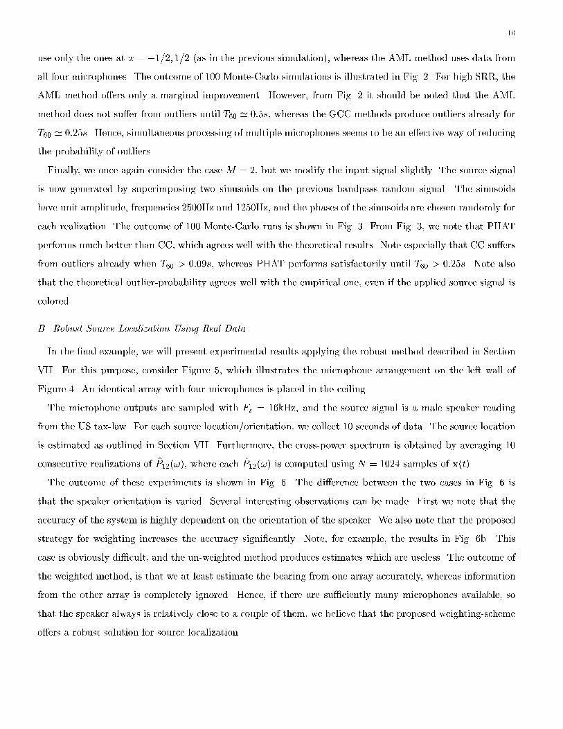
Consider next Fig. 1. The predicted expressions for the CRB and the probability of an outlier show a

good agreement with the empirical accuracy. The empirical variance of the GCC methods follows closely

their theoretical counterparts. It is interesting to note that for T60 small, the de�nition �(T60) = 2=T60 seems

accurate, whereas the de�nition �(T60) = 7=T60 seems more accurate for larger reverberation times. However,

when T60 > 0:1s, the probability of outliers becomes dominant, and the estimation error is no longer tolerable.

The AML estimator reaches the CRB only for small values of T60, and su�ers also from outliers. Hence, in

this case there seems to be no bene�ts from using AML.

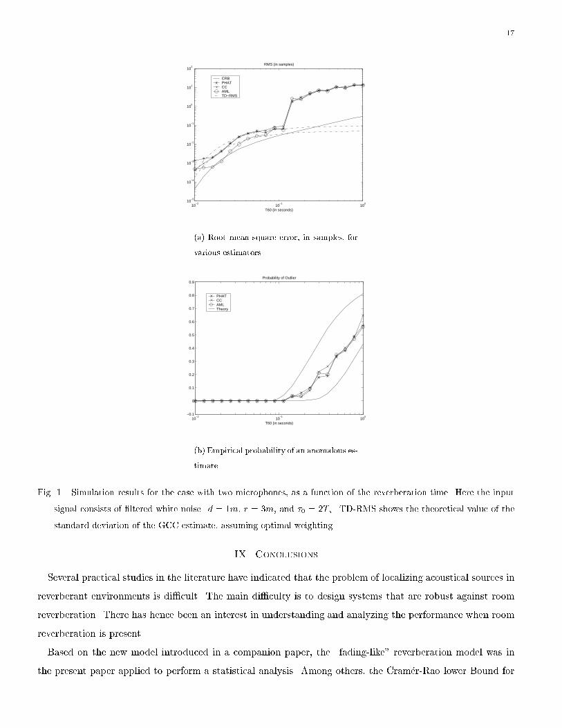
Next we consider a possible remedy for decreasing the probability of an outlier. The scenario is identical

to the previous one, i.e. d = 1m. However, we now include two additional microphones in-between the two

previous ones, i.e. along the x-axis there are microphones at x = �1=2;�1=3; 1=3; 1=2 m. The GCC methods

16

use only the ones at x = �1=2; 1=2 (as in the previous simulation), whereas the AML method uses data from

all four microphones. The outcome of 100 Monte-Carlo simulations is illustrated in Fig. 2. For high SRR, the

AML method o�ers only a marginal improvement. However, from Fig. 2 it should be noted that the AML

method does not su�er from outliers until T60 ' 0:5s, whereas the GCC methods produce outliers already for

T60 ' 0:25s. Hence, simultaneous processing of multiple microphones seems to be an e�ective way of reducing

the probability of outliers.

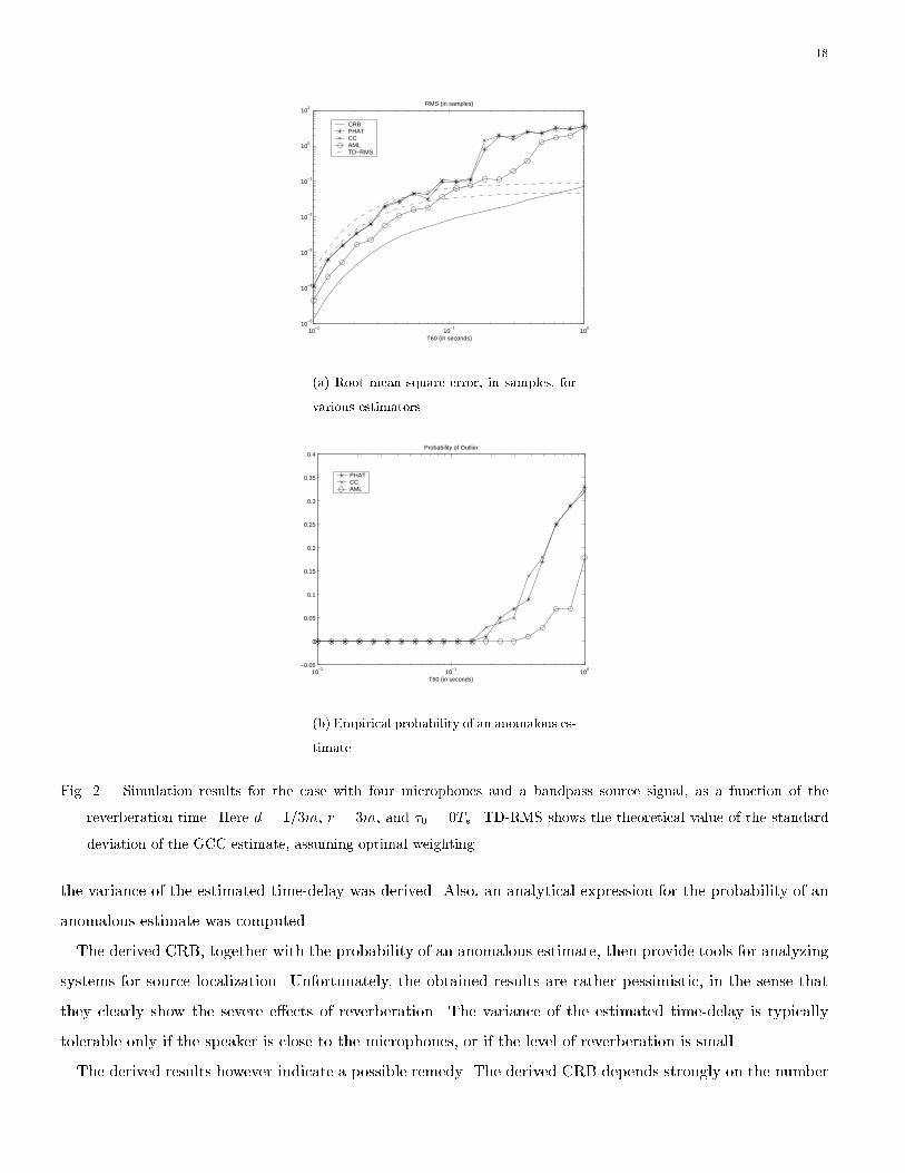
Finally, we once again consider the case M = 2, but we modify the input signal slightly. The source signal

is now generated by superimposing two sinusoids on the previous bandpass random signal. The sinusoids

have unit amplitude, frequencies 2500Hz and 1250Hz, and the phases of the sinusoids are chosen randomly for

each realization. The outcome of 100 Monte-Carlo runs is shown in Fig. 3. From Fig. 3, we note that PHAT

performs much better than CC, which agrees well with the theoretical results. Note especially that CC su�ers

from outliers already when T60 > 0:09s, whereas PHAT performs satisfactorily until T60 > 0:25s. Note also

that the theoretical outlier-probability agrees well with the empirical one, even if the applied source signal is

colored.

B. Robust Source Localization Using Real Data

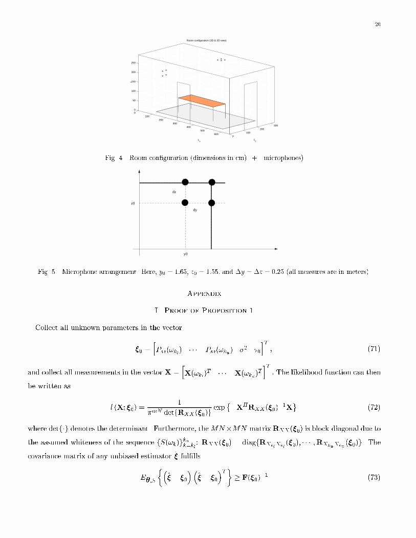
In the �nal example, we will present experimental results applying the robust method described in Section

VII. For this purpose, consider Figure 5, which illustrates the microphone arrangement on the left wall of

Figure 4. An identical array with four microphones is placed in the ceiling.

The microphone outputs are sampled with Fs = 16kHz, and the source signal is a male speaker reading

from the US tax-law. For each source location/orientation, we collect 10 seconds of data. The source location

is estimated as outlined in Section VII. Furthermore, the cross-power spectrum is obtained by averaging 10

consecutive realizations of P12(!), where each P12(!) is computed using N = 1024 samples of x(t).

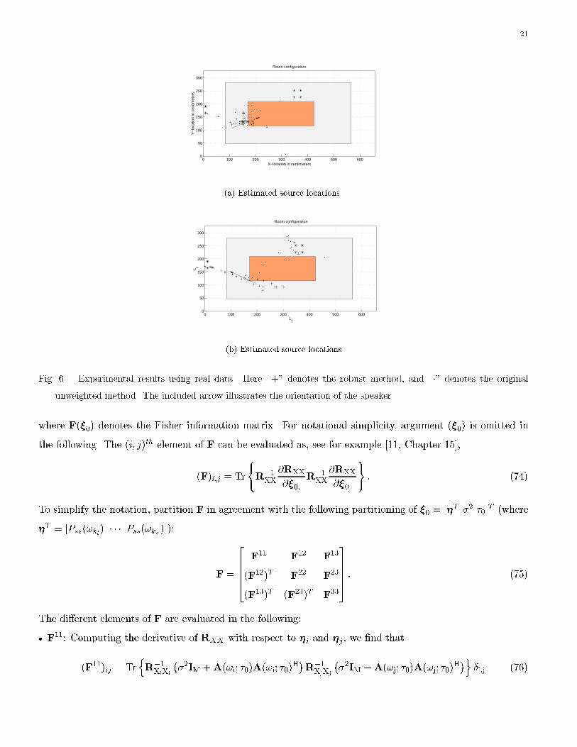
The outcome of these experiments is shown in Fig. 6. The di�erence between the two cases in Fig. 6 is

that the speaker orientation is varied. Several interesting observations can be made. First we note that the

accuracy of the system is highly dependent on the orientation of the speaker. We also note that the proposed

strategy for weighting increases the accuracy signi�cantly. Note, for example, the results in Fig. 6b. This

case is obviously di�cult, and the un-weighted method produces estimates which are useless. The outcome of

the weighted method, is that we at least estimate the bearing from one array accurately, whereas information

from the other array is completely ignored. Hence, if there are su�ciently many microphones available, so

that the speaker always is relatively close to a couple of them, we believe that the proposed weighting-scheme

o�ers a robust solution for source localization.

17

10−2

10−1

100

10−5

10−4

10−3

10−2

10−1

100

101

102

T60 (in seconds)

RMS (in samples)

CRB PHAT CC AML TD−RMS

(a) Root mean square error, in samples, for

various estimators.

10−2

10−1

100

−0.1

0

0.1

0.2

0.3

0.4

0.5

0.6

0.7

0.8

0.9

T60 (in seconds)

Probability of Outlier

PHAT CC AML Theory

(b) Empirical probability of an anomalous es-

timate.

Fig. 1. Simulation results for the case with two microphones, as a function of the reverberation time. Here the input

signal consists of �ltered white noise. d = 1m, r = 3m, and �0 = 2Ts. TD-RMS shows the theoretical value of the

standard deviation of the GCC estimate, assuming optimal weighting.

IX. Conclusions

Several practical studies in the literature have indicated that the problem of localizing acoustical sources in

reverberant environments is di�cult. The main di�culty is to design systems that are robust against room

reverberation. There has hence been an interest in understanding and analyzing the performance when room

reverberation is present.

Based on the new model introduced in a companion paper, the \fading-like" reverberation model was in

the present paper applied to perform a statistical analysis. Among others, the Cram�er-Rao lower Bound for

18

10−2

10−1

100

10−5

10−4

10−3

10−2

10−1

100

101

T60 (in seconds)

RMS (in samples)

CRB PHAT CC AML TD−RMS

(a) Root mean square error, in samples, for

various estimators.

10−2

10−1

100

−0.05

0

0.05

0.1

0.15

0.2

0.25

0.3

0.35

0.4

T60 (in seconds)

Probability of Outlier

PHATCC AML

(b) Empirical probability of an anomalous es-

timate.

Fig. 2. Simulation results for the case with four microphones and a bandpass source signal, as a function of the

reverberation time. Here d = 1=3m, r = 3m, and �0 = 0Ts. TD-RMS shows the theoretical value of the standard

deviation of the GCC estimate, assuming optimal weighting.

the variance of the estimated time-delay was derived. Also, an analytical expression for the probability of an

anomalous estimate was computed.

The derived CRB, together with the probability of an anomalous estimate, then provide tools for analyzing

systems for source localization. Unfortunately, the obtained results are rather pessimistic, in the sense that

they clearly show the severe e�ects of reverberation. The variance of the estimated time-delay is typically

tolerable only if the speaker is close to the microphones, or if the level of reverberation is small.

The derived results however indicate a possible remedy. The derived CRB depends strongly on the number

19

10−2

10−1

100

10−5

10−4

10−3

10−2

10−1

100

101

102

T60 (in seconds)

RMS (in samples)

CRB PHAT CC AML TD−RMS

(a) Root mean square error, in samples, for

various estimators.

10−2

10−1

100

−0.1

0

0.1

0.2

0.3

0.4

0.5

0.6

0.7

0.8

0.9

T60 (in seconds)

Probability of Outlier

PHAT CC AML Theory

(b) Empirical probability of an anomalous es-

timate.

Fig. 3. Simulation results for the case with two microphones, as a function of the reverberation time. Here the input

signal consists of �ltered white noise with two superimposed sinusoids. d = 1m, r = 3m, and �0 = 2Ts. TD-RMS

shows the theoretical value of the standard deviation of the GCC estimate, assuming optimal weighting.

of microphones used to estimate the bearing. Hence, a more complete study of the attainable accuracy when

several microphones simultaneously are processed is highly desired. Another possibility for designing more

robust estimators, is to combine audio and video information. The main idea then is to use video information

to provide initial estimates of the positions of potential speakers. Then it should be possible to decrease

the probability of anomalous estimates, by properly incorporating the video-information. For example, the

video-information can tell us in which range the true time-delay should be found, which potentially could

decrease the probability of an anomalous estimate.

20

0100

200300

400500

6000

100200

300

0

50

100

150

200

250

Ly

Room configuration (3D & 2D view)

Lx

z

Fig. 4. Room con�guration (dimensions in cm). + - microphones)

y0

z0

dz

dy

Fig. 5. Microphone arrangement. Here, y0 = 1:65, z0 = 1:55, and �y = �z = 0:25 (all measures are in meters).

Appendix

I. Proof of Proposition 1

Collect all unknown parameters in the vector

�0 =hPss(!kl) � � � Pss(!ku) �2 �0

iT; (71)

and collect all measurements in the vector X =hX(!kl)

T � � � X(!ku)T

iT: The likelihood function can then

be written as

l (X; �0) =1

�mN detfRXX(�0)gexp

��XH

RXX(�0)�1X

(72)

where detf�g denotes the determinant. Furthermore, theMN�MN matrixRXX(�0) is block-diagonal due to

the assumed whiteness of the sequence fS(!k)gkuk=kl

: RXX(�0) = diagfRXklXkl

(�0); � � � ;RXkuXku(�0)g. The

covariance matrix of any unbiased estimator � ful�lls

E�;S

��� � �0

��� � �0

�T�� F(�0)

�1 (73)

21

0 100 200 300 400 500 6000

50

100

150

200

250

300

X−location in centimeters

Y−

loca

tion

in c

entim

eter

s

Room configuration

(a) Estimated source locations.

0 100 200 300 400 500 6000

50

100

150

200

250

300

Lx

L y

Room configuration

(b) Estimated source locations.

Fig. 6. Experimental results using real data. Here \+" denotes the robust method, and \�" denotes the original

unweighted method. The included arrow illustrates the orientation of the speaker.

where F(�0) denotes the Fisher information matrix. For notational simplicity, argument (�0) is omitted in

the following. The (i; j)th element of F can be evaluated as, see for example [11, Chapter 15],

(F)i;j = Tr

(R�1XX

@RXX

@�0iR�1XX

@RXX

@�0j

): (74)

To simplify the notation, partition F in agreement with the following partitioning of �0 = [�T �2 �0]T (where

�T = [Pss(!kl) � � � Pss(!ku)]):

F =

26664F11

F12

F13

(F12)T F22

F23

(F13)T (F23)T F33

37775 : (75)

The di�erent elements of F are evaluated in the following:

� F11: Computing the derivative of RXX with respect to �i and �j, we �nd that

(F11)ij = TrnR�1XiXi

��2IM +A(!i; �0)A(!i; �0)

H�R�1XjXj

��2IM +A(!j; �0)A(!j; �0)

H�o

�i;j (76)

22

where �i;j denotes Kronecker's delta function. Using the matrix inversion lemma, it follows that

R�1XiXi

=1

�2Pss(!i)

�IM �

A(!i; �0)A(!i; �0)H

�2 +M

�; (77)

where we used the fact that A(!i; �0)HA(!i; �0) =M . The expression for (F11)ij then simpli�es to

(F11)ij =M

P 2ss(!i)

�i;j ; (78)

and �nally

F11 = diag

�M

P 2ss(!kl)

; � � � ;M

P 2ss(!ku)

�: (79)

� F22: Since the derivative of RXiXi

with respect to �2 equals Pss(!i)IM ,

F22 =

kuXk=kl

P 2ss(!i)Tr

nR�2XiXi

o: (80)

If we once again apply expression (77), straightforward calculations result in the following expression:

F22 =

MN

�4

�1�

2

�2 +M+

M

(�2 +M)2

�: (81)

� F33: Next we compute the derivative of RXiXi

with respect to the time-delay �0. We then �nd that

@

@�0RXiXi

= Pss(!i)Di; (82)

where

Di4=

@

@�0A(!i; �0)A(!i; �0)

H = A(!i; �0)DH(!i; �0) +D(!i; �0)A

H(!i; �0) (83)

D(!i; �0) =@A(!i; �0)

@�0: (84)

It is then easy to see that

F33 =

1

�4

kuXk=kl

Tr fPkDkPkDkg ; (85)

where

Pk4= IM �

A(!k; �0)AH(!k; �0)

�2 +M: (86)

� Along the same lines, it can be shown that

F12 =

M

�2

�1�

1

�2 +M

��1

Pss(!kl); � � � ;

1

Pss(!ku)

�T(87)

F13 =

1

�2[TrfPklDklg; � � � ;TrfPkuDkug]

T (88)

F23 =

1

�4

kuXk=kl

Tr fPkDkPkg : (89)

23

To simplify the CRB expression, we next note that F13 = 0. This follows since

TrfPiDig =�2

�2 +M

�TrfA(!i; �0)D(!i; �0)

Hg+TrfD(!i; �0)A(!i; �0)Hg�

(90)

=�2

�2 +M

j!i

M�1Xl=1

l

!+

j!i

M�1Xl=1

l

!�!= 0: (91)

Similarly it can be shown that F23 = 0. Hence, the expression for F reads as

F =

26664F11

F12

0

(F12)T F22

0

0 0 F33

37775 ; (92)

and we �nally �nd that

E�;S

n(� � �0)

2o� (F33)�1: (93)

II. Proof of Proposition 2

For large N , the estimated cross-correlation can be written as

R(nTs) ' E fx1(t)x2(t� �);�g =1

N

N2�1X

k=�N2

P12(!k;�)ej!knTs ; (94)

where

P12(!k;�) = Rss

�e�j!kn0Ts +R2(!k;�) +R�1(!k;�)e

�j!kn0Ts +R2(!k;�)R�1(!k;�)

�; (95)

denotes the cross-power spectrum, conditioned on �. Here, R(!k;�) = [R1(!k;�) R2(!k;�)]T : Note, when

computing R(nTs), also frequencies that does not satisfy the Schroeder large room frequency are included in

the summation (94). We will however neglect this fact in the following.

We next proceed to determine the statistical properties of R(nTs). For that purpose, it is useful to �rst

determine the properties of P12(!k;�). Evaluating the expected value of P12(!k;�), we �nd that

E� fP12(!k;�)g = Rsse�j!kn0Ts : (96)

We can now show that the expected value of R(nTs) equals

E�

nR(nTs)

o=

8<: Rss for n = n0

0 for n 6= n0: (97)

To see this, note that

E�

nR(nTs)

o=

Rss

N

N2�1X

k=�N2

ej(n�n0)!kTs =Rss

N

N2�1X

k=�N2

ej(n�n0)2�kN : (98)

24

Result (97) then follows from the orthogonality properties of complex sinusoids.

Next we would like to compute the variance of R(nTs). Keeping in mind that Var�fR(nTs)g = E�fR2(nTs)g�

E2�fR(nTs)g, we study

E�

nR2(nTs)

o=

1

N2

Xk;l

E� fP12(!k;�)P�12(!l;�)g e

j(!k�!l)nTs

=1

N2

Xk 6=l

E� fP12(!k;�)P�12(!l;�)g e

j(!k�!l)nTs +1

N2

Xk=l

E� fP12(!k;�)P�12(!k;�)g :

(99)

For !k 6= !l we �nd that

E� fP12(!k;�)P�12(!l;�)g �E�

nP12(!k)

oE�;S

nP12(!l)

�o

= R2ssE�

��e�j!kn0Ts +R2(!k;�) +R�1(!k;�)e

�j!kn0Ts +R2(!k;�)R�1(!k;�)

��e�j!ln0Ts +R2(!l;�) +R�1(!l;�)e

�j!ln0Ts +R2(!l;�)R�1(!l;�)

��o�R2

ssejn0Ts(!l�!k):

(100)

De�ning the quantity (for explicit expressions, see [7])

(!k � !l)4= E� fR1(!k;�)R1(!l;�)

�g = E� fR2(!k;�)R2(!l;�)�g ; (101)

equation (100) can be written as

E�;S

nP12(!k)P

�12(!l)

o�E�;S

nP12(!k)

oE�;S

nP12(!l)

�o

= R2ss

�(!k � !l) + (!k � !l) e

jn0Ts(!l�!k) +(!k � !l)2�:

(102)

The technical complication in the analysis is that terms like (!k � !l) 6= 0 due to the frequency correlation

of R(!;�). The analysis can in principle be carried out using the function (!k � !l). We choose however a

simpler, but approximative, approach. The main observation is that R(nTs) for large N approximately can

be written as

R(nTs) '1~N

~N2�1X

k=�~N2

P12(�k;�)ej�knTs ; (103)

where we have re-sampled the frequency axis according to the coherence bandwidth �(T60) of R(!;�):

�k =2�Fs~N

; k = �~N

2; � � � ;

~N

2� 1 (104)

~N =Fs

�(T60): (105)

The approximation (103) is based on the fact that P12(!k;�) and P12(!l;�) are highly correlated for a small

frequency separation j!k�!lj. In the following it will be assumed that (�) is negligible for j!k�!lj � 2��(T60).

We then �nd that

E� fP12(�k;�)P�12(�l;�)g =

8<: R2

ss

�1 + 1

SRR

�2for �k = �l

R2sse

jn0Ts(�l��k) for �k 6= �l; (106)

25

and

E� fP12(�k;�)P�12(�l;�)g �E� fP12(�k;�)gE� fP12(�l;�)

�g = 0 for �k 6= �l: (107)

Returning to equation (99), we �nd that

E�

nR2(nTs)

o'

R2ss

~N2

Xk 6=l

ej(�k��l)(n�n0)Ts +1~NR2ss

�1 +

1

SRR

�2

= R2ss

~N � 1~N

�n�n0 �R2ss

~N(1� �n�n0) +

1~NR2ss

�1 +

1

SRR

�2

= R2ss�n�n0 +

1~NR2ss

�1 +

1

SRR

�2

�R2ss

~N:

(108)

Since E�fR(nTs)g = Rss�n�n0 , it consequently follows that

Var�

nR(nTs)

o'

1~NR2ss

�1 +

1

SRR

�2

�R2ss

~N=

R2ss

~N

�2

SRR+

1

SRR2

�: (109)

The proof is complete if we can establish that R(n1Ts) and R(n2Ts) are independent for n1 6= n2, and

that R(nTs) is Gaussian for all n. The Gaussianity follows from the central limit theorem, since we assume

~N � m. Finally, we would like to establish that R(n1Ts) and R(n2Ts) are uncorrelated. Details are omitted,

but calculations completely analogous to the previous ones (and invoking the approximation (103), show that

for n1 6= n2

E�

n�R(n1Ts)�E�

nR(n1Ts)

o��R(n2Ts)�E�

nR(n2Ts)

o�o' 0; (110)

as required.

References

[1] J.B. Allen and A. Berkeley. "Image Method for E�ciently Simulating Small-room Acoustics". Journal of the Acoustical

Society of America, 65(4):943{950, April 1979.

[2] M. S. Brandstein, J. E. Adcock, and H. F. Silverman. "A Closed-Form Estimator for use with Room Environment Microphone

Arrays". IEEE Trans. on Speech and Audio Processing, 5(1):45{50, January 1997.

[3] M.S. Brandstein. "A Pitch-based Approach to Time-delay Estimation of Reverberant Speech". In IEEE ASSP Workshop on

Applications of Signal Processing to Audio and Acoustics, New Paltz, NY, 1997.

[4] M.S Brandstein and H.F. Silverman. "A Practical Methodology for Speech Source Localization with Microphone Arrays".

Computer, Speech, and Language, 11(2):91{126, April 1997.

[5] B. Champagne, S. B�edard, and A. St�ephenne. "Performance of Time-delay Estimation in the Presence of Room Reverbera-

tion". IEEE Trans. on Speech and Audio Processing, 4(2):148{152, March 1996.

[6] M.A. Doron, A.J. Weiss, and H. Messer. "Maximum-Likelihood Direction Finding of Wide-Band Sources". IEEE Trans. on

Signal Processing, 1(2):411{417, January 1993.

[7] T. Gustafsson and B.D. Rao. "Source Localization in Reverberant Environments: Modeling". Submitted to IEEE Trans. on

Speech and Audio Processing for possible publication, 2000.

26

[8] J.P. Ianniello. "Time Delay Estimation Via Cross-Correlation in the Presence of Large Estimation Errors". IEEE Trans. on

Acoustics, Speech, and Signal Processing, 30(6):998{1003, December 1982.

[9] J.P. Ianniello. "High-resolution Multipath Time Delay Estimation for Broadband Random Signals". IEEE Trans. on Acous-

tics, Speech, and Signal Processing, 36(3):320{327, March 1988.

[10] E.E. Jan and J. Flanagan. "Sound Source Localization in Reverberant Environments using an Outlier Elimination Algorithm".

In Proc. of ICSLP, pages 1321{4, Philadelphia, USA, 1996.

[11] S. M. Kay. Fundamentals of Statistical Signal Processing. Prentice-Hall, Englewood Cli�s, NJ, 1993.

[12] C.H. Knapp and G.C. Carter. "The Generalized Correlation Method for Estimation of Time Delay". IEEE Trans. on

Acoustics, Speech, and Signal Processing, 24(4):320{326, August 1976.

[13] H. Kuttru�. Room Acoustics. John Wiley, 1973.

[14] L. Ljung. System Identi�cation: Theory for the User. Prentice-Hall, Englewood Cli�s, NJ, 1987.

[15] M. Omologo and P. Svaizer. "Acoustic Source Location in Noisy and Reverberant Environment Using CSP Analysis". In

Proc. ICASSP, pages 921{924, Atlanta, USA, 1996.

[16] M. Omologo and P. Svaizer. "Use of the Crosspower-Spectrum Phase in Acoustic Event Localization". IEEE Trans. on

Speech and Audio Processing, 5(3):288{292, May 1997.

[17] H. C. Schau and A. Z. Robinson. "Passive Source Localization Employing Intersecting Spherical Surfaces from Time-of-Arrival

Di�erences". IEEE Trans. on Acoustics, Speech, and Signal Processing, 35(8):1223{1225, August 1987.

[18] J.O. Smith and J.S. Abel. "Closed-Form Least-Squares Source Location Estimation from Range-Di�erence Measurements".

IEEE Trans. on Acoustics, Speech, and Signal Processing, 35(12):1661{1669, December 1987.

[19] P. Stoica and A. Nehorai. "Performance Study of Conditional and Unconditional Direction-of-arrival Estimation". IEEE

Trans. on Acoustics, Speech and Signal Processing, 38(10):1783{95, Oct. 1990.