1

Statistics, Data Analysis and Image Processing

Lectures 9 10 11

Vlad Stolojan

Advanced Technology Institute

University of Surrey

2

Learning Outcomes

- how to calculate experimental errors

- image processing

- filtering

- thresholding

- particle analysis.

- data analysis

- fitting peaks

- filtering

- displaying

3

The labbook

• Date, title

• Aim of the experiment

• Description of the apparatus (brief), arrangement (sketch)

• Experimental method (main steps, precautions)

• Measurements (if recorded), environmental parameters

• Graphs + Calculations

• Conclusions (brief).

Number pages.

4

Experimental results

• Repeatability

• Calculations = levels of confidence

(eg. Organic solar cell with 8% efficiency ± ?).

• Uncertainties in measurements = significant figures:

3.14 ± 0.1 3.14 ± 0.12 3.14 ± 0.124

• SI UNITS – always check your formula. (particularly in exam).

5

True value, Accuracy, Precision

• True value: when measuring we estimate the exact, true value. The more measurements, the closer the mean of these is to the true value.

• Accurate: close to the true value.

• Precise: small uncertainty bu not necessarily close to the true value.

Accurate and Precise

6

Error Propagation

• If a has uncertainty Δa and b has uncertainty Δb, then the uncertainty of a function of a and b, may not be just Δa+Δb – Δa may be positive and Δb negative.

• What it means is that if:

f = f(a,b) then Δf ≠ f(Δa,Δb)

• Variational calculus:

f 2 x1, x2 ... x n=∑i

∂ f∂ x i

2

x i2

7

Error propagation

• Young's modulus for a beam of length L0, area A0

which lengthens ΔL under force F

• What is the error in E. Clue: divide the error propagation equation by E.

E=F L0A0 L

8

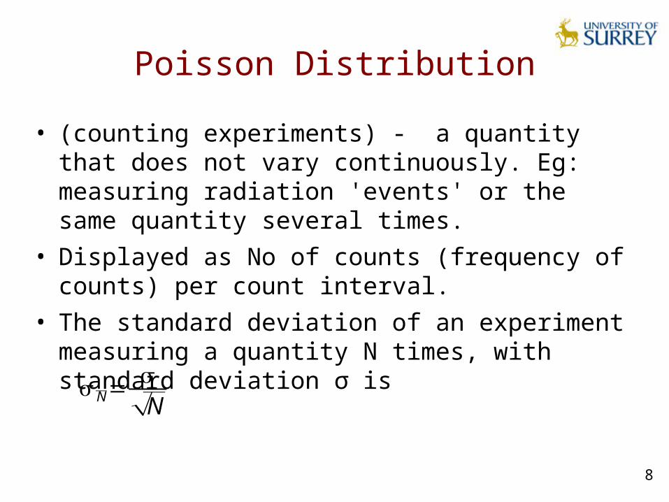
Poisson Distribution

• (counting experiments) - a quantity that does not vary continuously. Eg: measuring radiation 'events' or the same quantity several times.

• Displayed as No of counts (frequency of counts) per count interval.

• The standard deviation of an experiment measuring a quantity N times, with standard deviation σ is

N=N

9

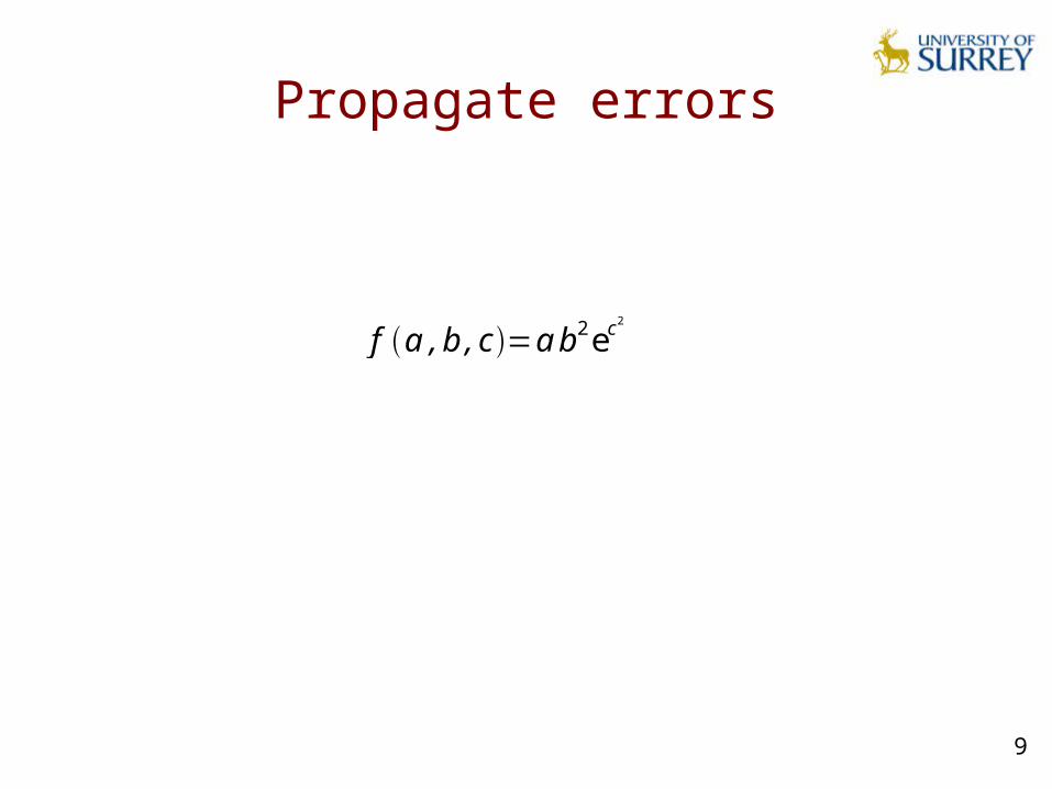
Propagate errors

f a , b , c=a b2ec2

10

Error propagation

• An amorphous square solar cell of dimensions (1.0±0.1) cm is illuminated with (0.155 ± 0.001) W.

The maximum current density measured from the device is Jm= (18.9 ± 0.1) mA/cm2 and maximum

voltage is Vm= (0.950 ± 0.001) V. What is the

efficiency of the device and the error?

11

Peak position

• A spectrum = counts per energy/ frequency/ wavelength interval – Poisson statistics.

• The standard deviation in the position of a peak scales with 1/√N (no. of data points used in fitting).

• We can compare peak-shift positions say to 20-30meV even when the energy interval (sampling resolution) is 200meV. How many data points? What energy interval?

12

Mean, Median, Mode, Skewness, etc

• Mean = sum of observations / no. of observations

(the expected value).

• Median = the number separating the higher half of observations from the lower half of observations.

• Mode = the value that occurs most frequently.

• Skewness = asymmetry of the distribution. Negative – long left tail, positive – longer right tail.

• Kurtosis (bulging -greek) : high: sharp peak with fat tails vs low: rounded peak with thin tails.

13

Image processing and analysis

• Intensity histograms; Histogram transformations.

• Geometric transformations: scaling, rotation, interpolation, binning.

• Color images.

• Filtering

• Particle analysis

• Bi-variate tri-variate histograms.

14

Intensity Histogram. Transformations

num

ber

of p

ixel

s

0

5000

10000

15000

20000

num

ber

of p

ixel

s

20000 25000 30000 35000 40000 45000 50000 55000 60000 65000

num

ber

of p

ixel

s

0

1000

2000

3000

4000

5000

6000

7000

8000

9000

10000

11000nu

mbe

r of

pix

els

0 50 100 150 200 250

15

Intensity Histogram. Transformations

num

ber

of p

ixel

s

0

1000

2000

3000

4000

5000

6000

7000

8000

9000

10000

11000

num

ber

of p

ixel

s50 100 150 200 250

num

ber

of p

ixel

s

0

1000

2000

3000

4000

5000

6000

7000

8000

9000

10000

11000nu

mbe

r of

pix

els

0 50 100 150 200 250

16

Interpolation and Resampling

• Interpolation: • Nearest-neighbour: assign the value of the nearest

pixel• Bilinear: weighted sum of the 4 nearest pixels.

• Resampling (binning) combine two or more pixels into a weighted average → decrease of resolution but faster read-out. Can be done on CCD capture device.

17

Colour

• RGB = (red, green, blue) : vector; each component 0-255.

• CMY, CMYK (blacK)

Magenta

Cyan

Yellow

18

Filtering

• Filtering = used for smoothing, noise reduction or for emphasizing a pattern/feature.

• Convolution

f ⊗g x=∫ f y g x− y dyFT f ⊗g =FT f FT g

19

Filtering

• Smooth

• Sharpen

• Band pass

• Edge detection

20

Particle analysis

1) Flat-fielding (uniform illumination, uniform response)

2) Filtering + binarization (convert grey scale to black-white).

3) Thresholding (select information)

4) Analyze particles.

http://rsb.info.nih.gov/ij/index.htm

ImageJPlugins

21

Graphs

• Usually all data should look good represented in an image a journal column-wide. Font min 11, size 8.5 x (up to a page length) cm.

• Minimise empty space (scaling, etc)

• Captions caption captions!• Descriptive and informative. The reader should not

need to refer to the text to understand what is shown in the graph.

• Definitely NOT 'plot of this vs that'

22

Examples of captions

23

Examples of captions