1

STMAS:Space-Time Mesoscale Analysis System

Steve Koch, John McGinley, Yuanfu Xie, Steve Albers, Ning Wang, Patty Miller

2

• Create a mesoscale analysis that:• Assimilates all available surface data at high time

frequency• Performs data quality control • Has a very rapid product cycle (< 15 minutes)• Can sustain features with typical mesoscale structure (gust

fronts, gravity waves, bores, sea breezes, etc)• Can be used for boundary identification and monitoring

(SPC)• Candidate for automated processing

• Is compatible with current workstation technology

STMAS Goal

3

• Surface Observations• Meteorological Aviation Reports (METARs)• Coastal Marine Automated Network (C-MAN)• Surface Aviation Observations (SAOs)• Modernized Cooperative Observer Program (COOP)• Many mesonetworks (constantly growing)

• MADIS offers automated Quality Control• Gross validity checks• Temporal consistency checks• Internal (physical) consistency checks• Spatial (“buddy”) checks

• MADIS Home Page: www-sdd.fsl.noaa.gov/MADIS

• Real-Time Display: www-frd.fsl.noaa.gov/mesonet/

STMAS utilizes surface data available through the FSL Meteorological Assimilation Data Ingest System (MADIS)

4

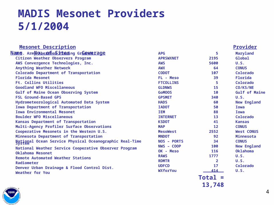
MADIS Mesonet Providers 5/1/2004

Mesonet Description Provider Name No. of Sites Coverage

Total = 13,748

U.S. Army Aberdeen Proving GroundsCitizen Weather Observers ProgramAWS Convergence Technologies, Inc.Anything Weather NetworkColorado Department of TransportationFlorida MesonetFt. Collins UtilitiesGoodland WFO MiscellaneousGulf of Maine Ocean Observing SystemFSL Ground-Based GPSHydrometeorological Automated Data SystemIowa Department of TransportationIowa Environmental MesonetBoulder WFO MiscellaneousKansas Department of TransportationMulti-Agency Profiler Surface ObservationsCooperative Mesonets in the Western U.S.Minnesota Department of TransportationNational Ocean Service Physical Oceanographic Real-Time SystemNational Weather Service Cooperative Observer ProgramOklahoma MesonetRemote Automated Weather StationsRadiometerDenver Urban Drainage & Flood Control Dist.Weather for You

APGAPRSWXNETAWSAWXCODOTFL - MesoFTCOLLINSGLDNWSGoMOOSGPSMETHADSIADOTIEMINTERNETKSDOTMAPMesoWestMNDOTNOS – PORTSNWS – COOPOK - MesoRAWSRDMTRUDFCDWXforYou

MarylandGlobalU.S.CONUSColoradoFloridaColoradoCO/KS/NEGulf of MaineU.S.New EnglandIowaIowaColoradoKansasCONUSWest CONUSMinnesotaCONUSNew EnglandOklahomaU.S.U.S.ColoradoU.S.

521955600

64107395

1510

340605088134112

25529234

100116

17772

17414

5

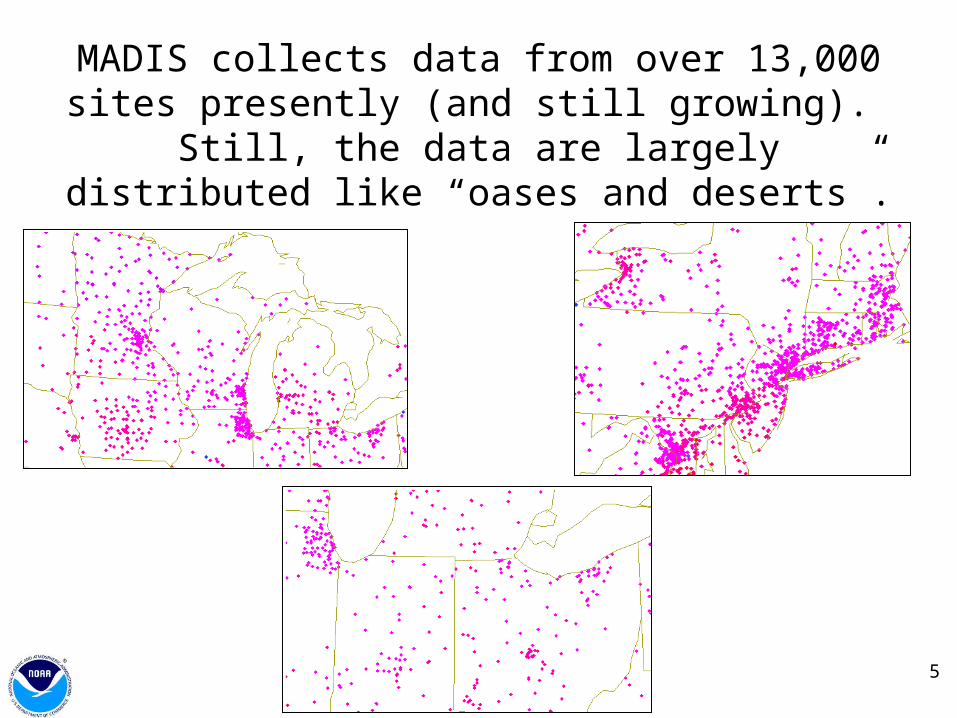
MADIS collects data from over 13,000 sites presently (and still growing). Still, the data are

largely distributed like “oases and deserts”.

6

Why conventional objective analysis schemes are inadequate to deal with the desert-oasis problem

Successive correction (SC) schemes (e.g., Barnes used in LAPS) and optimum interpolation (OI) schemes (e.g., as used in MADIS RSAS/MSAS) suffer from common problems:

1. Inhomogeneous station distributions cause problems for a fixed value of the final weighting function or the covariance function scale

2. SC and OI schemes will introduce noise in the deserts if forced to try to show details that are resolvable in the data oases everywhere

3. None of the SC or OI schemes include the high-resolution time information explicitly, with the exception of the modified Barnes scheme of Koch and Saleeby (2001), which required assumptions about the advection vectors in time-to-space conversion approach

7

STMAS solution: Multi-scale space and time analysis capability

• Ability to represent large scales resolvable by the data distribution characteristic of the desert regions

• Two schemes tested: telescopic recursive filter and wavelet fitting• Recursive filter uses residual remaining after removal of the large-

scale component for telescopic analysis:– Compute residual reduce the filter scale do analysis of residuals at

this next smaller scale repeat N times until analysis error falls below the expected error in observations (N = 3-6)

– Include temporal weight in similar manner for the recursive filter– Variational cost function assures fit to observations

• Wavelet fitting technique provides for locally variable levels of detail, non-isotropic searching, and temporal weighting (still under development, though tested on analytic functions)

8

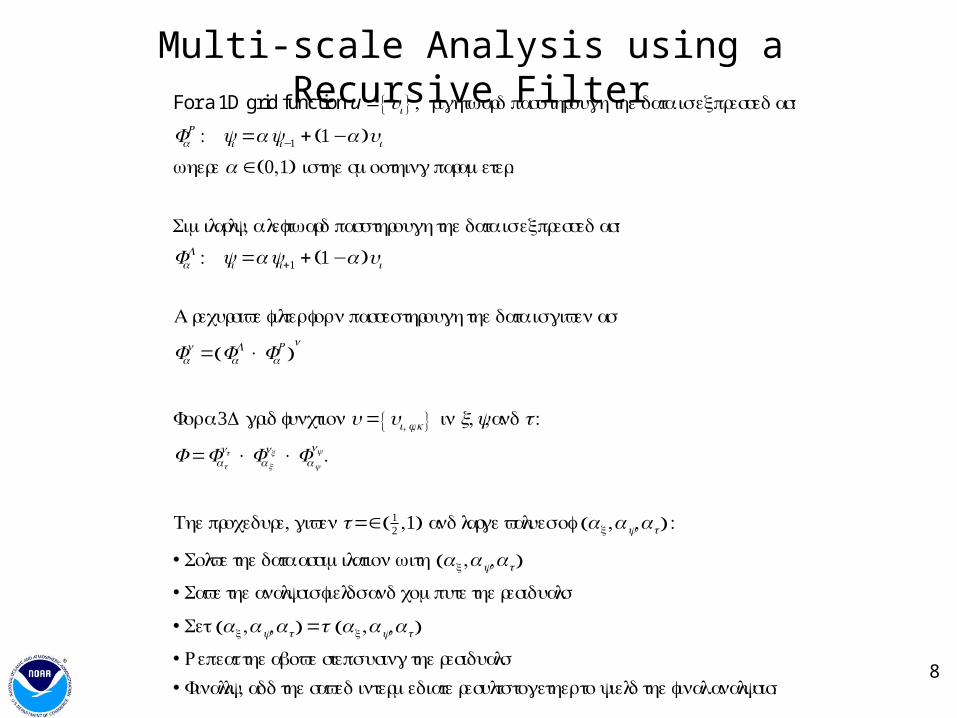
For a 1D grid function u = ui{ } , rightward pass through the data is expressed as:

FαR : yi =αyi−1 + 1−α( )ui

where α ∈ 0,1( ) is the smoothing parameter.

Similarly, a leftward pass through the data is expressed as:

FαL : yi =αyi+1 + 1−α( )ui

A recursive filter for n passes through the data is given as

Fαn = Fα

L ×FαR( )

n

For a 3D grid function u= ui, j ,k{ } in x,y,and t :

F =Fαt

nt ×Fαx

nx ×Fαy

ny .

The procedure, given τ=∈ 12 ,1( ) and large values of αx,αy,αt( ) :

• Solve the data assimilation with αx,αy,αt( )

• Save the analysis fields and compute the residuals

• Set αx,αy,αt( ) =τ αx,αy,αt( )

• Repeat the above steps using the residuals

• Finally, add the saved intermediate results together to yield the final analysis.

Multi-scale Analysis using a Recursive Filter

9

Comparisons of hourly analyses of temperature and winds using

LAPS and STMAS to surface and radar observations

Hourly analyses: 1900 - 2200 UTC

10

1900 UTC LAPS

11

2000 UTC LAPS

12

2100 UTC LAPS

13

2200 UTC LAPS

14

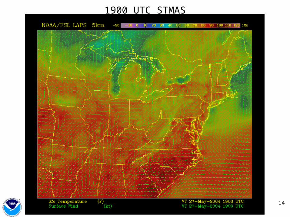
1900 UTC STMAS

15

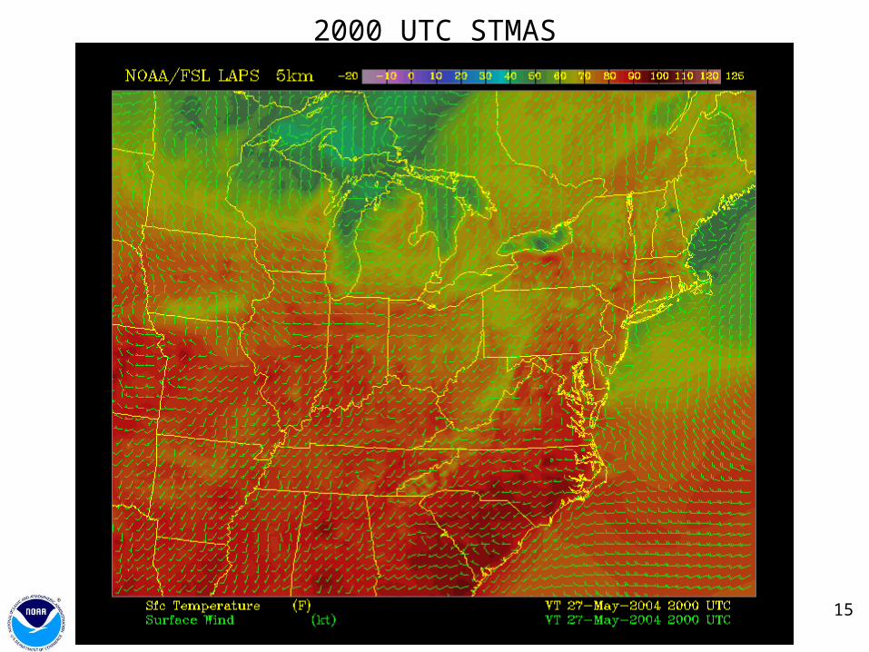
2000 UTC STMAS

16

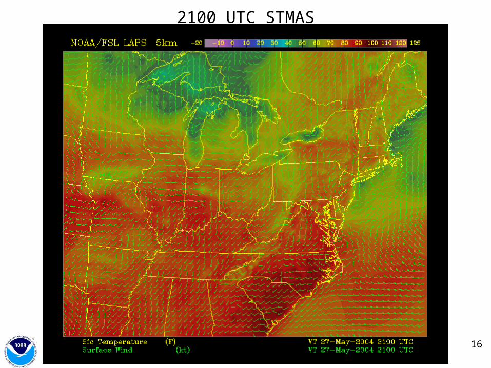
2100 UTC STMAS

17

2200 UTC STMAS

18

2155 UTC

19

Improvements to STMAS

• Use of Spline Wavelets– Accommodate common meteorological structures– Improve analysis in data rich and data sparse

areas

• Data Quality Control Using a Kalman Scheme– Operate in observation space– Provide data projections for future cycles– Optimum model for each station

20

Scattered data fitting using Spline Wavelets

• Basis functions: second order spline wavelets on bounded interval (by Chui and Quak)

• Penalty function in variational formulation: a weighted combination of least square error and magnitude of the high order derivatives

• Inner scaling functions control dilation and translation of the cardinal B-splines:

• Boundary scaling functions control dilation of the cardinal B-spline with multiple knots at the endpoints

21

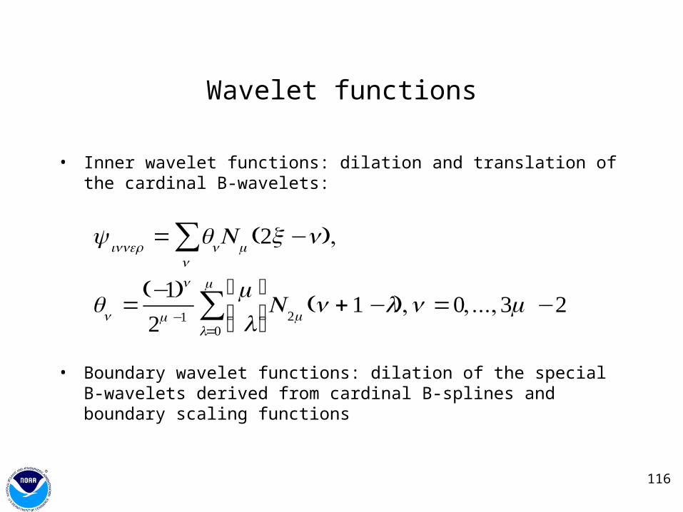
• Inner wavelet functions: dilation and translation of the cardinal B-wavelets

• Boundary wavelet functions: dilation of the special B-wavelets derived from cardinal B-splines and boundary scaling functions

Wavelet functions

22

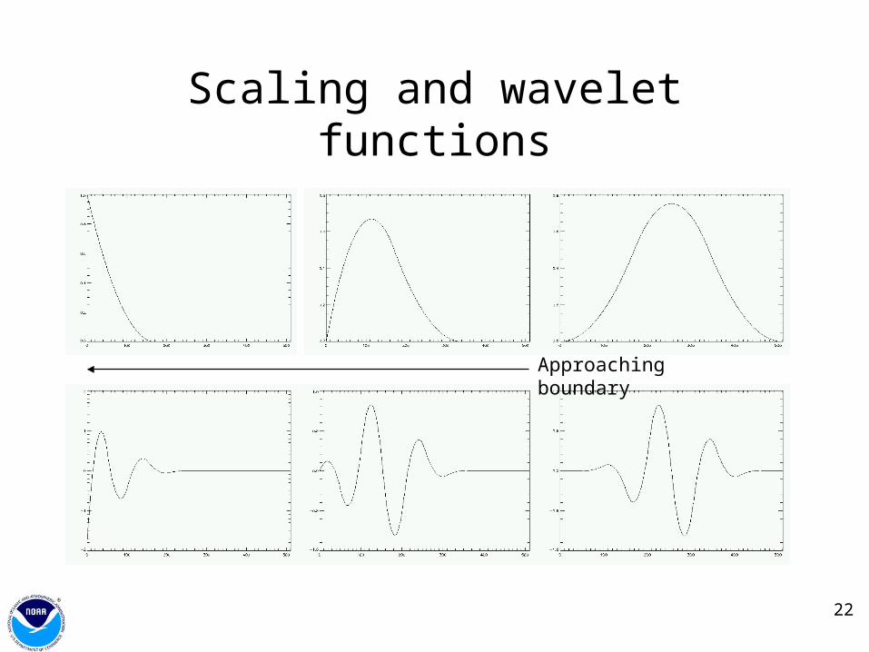
Scaling and wavelet functions

Approaching boundary

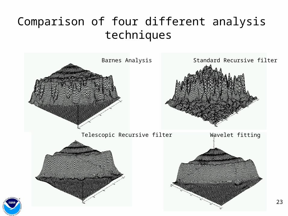
23

Comparison of four different analysis techniques

Barnes Analysis Standard Recursive filter

Telescopic Recursive filter Wavelet fitting

24

25

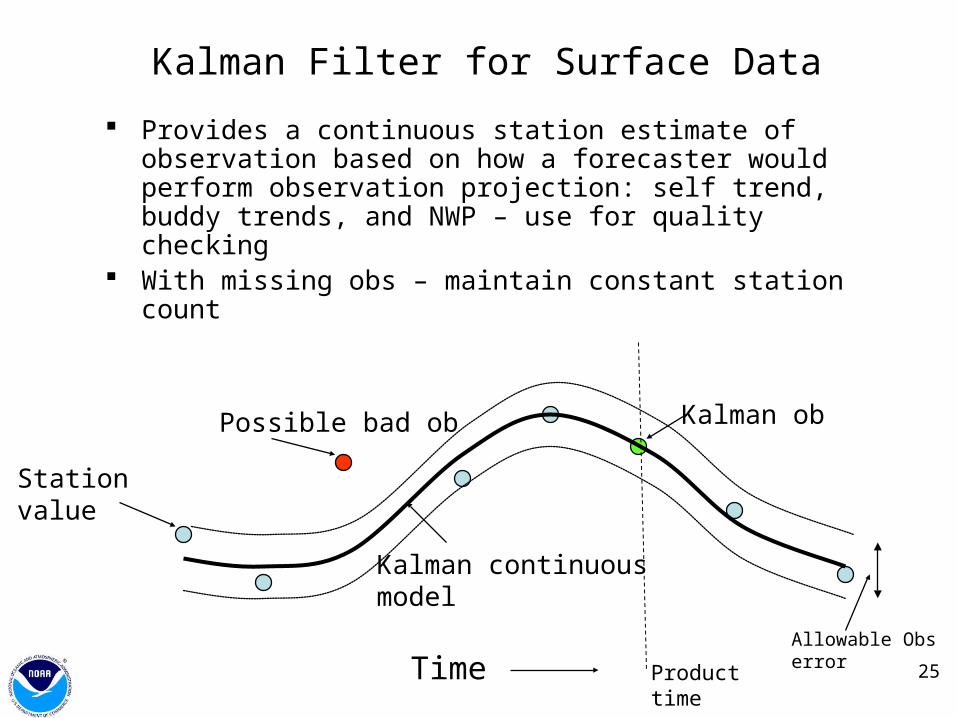
Kalman Filter for Surface Data

Provides a continuous station estimate of observation based on how a forecaster would perform observation projection: self trend, buddy trends, and NWP – use for quality checking

With missing obs – maintain constant station count

Time

Station value

Kalman ob

Kalman continuousmodel

Allowable Obserror

Possible bad ob

Producttime

26

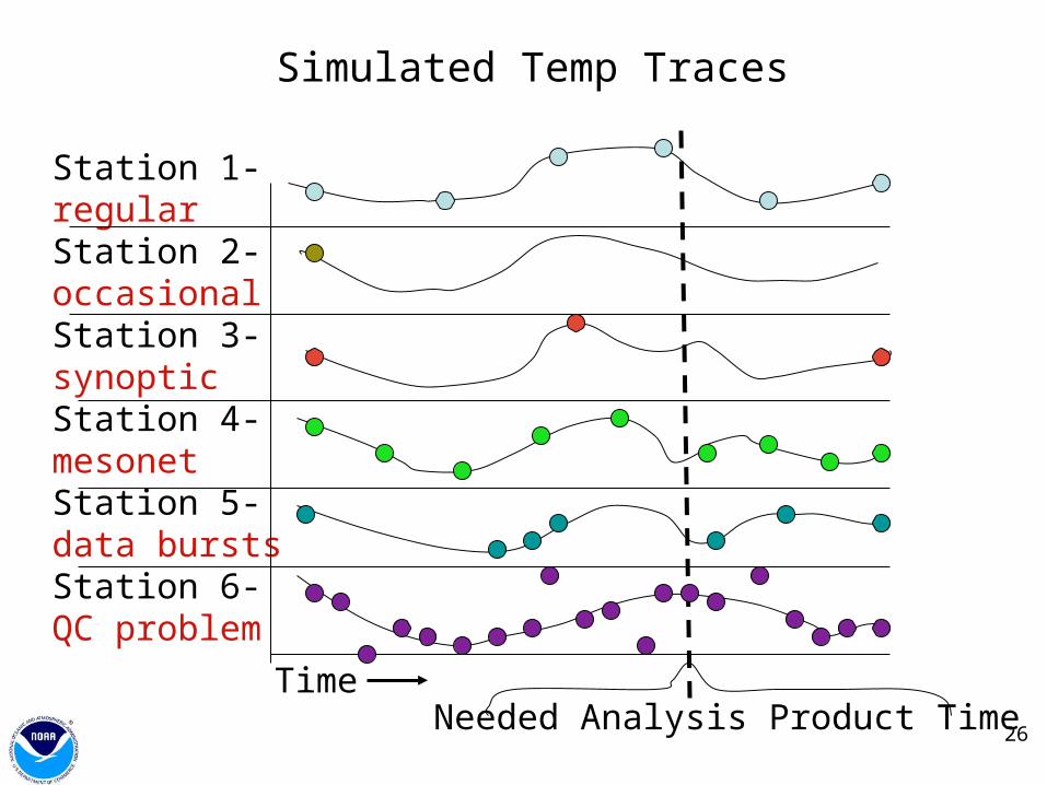
Simulated Temp Traces

Station 1-regularStation 2-occasionalStation 3-synopticStation 4-mesonetStation 5-data burstsStation 6-QC problem

Needed Analysis Product TimeTime

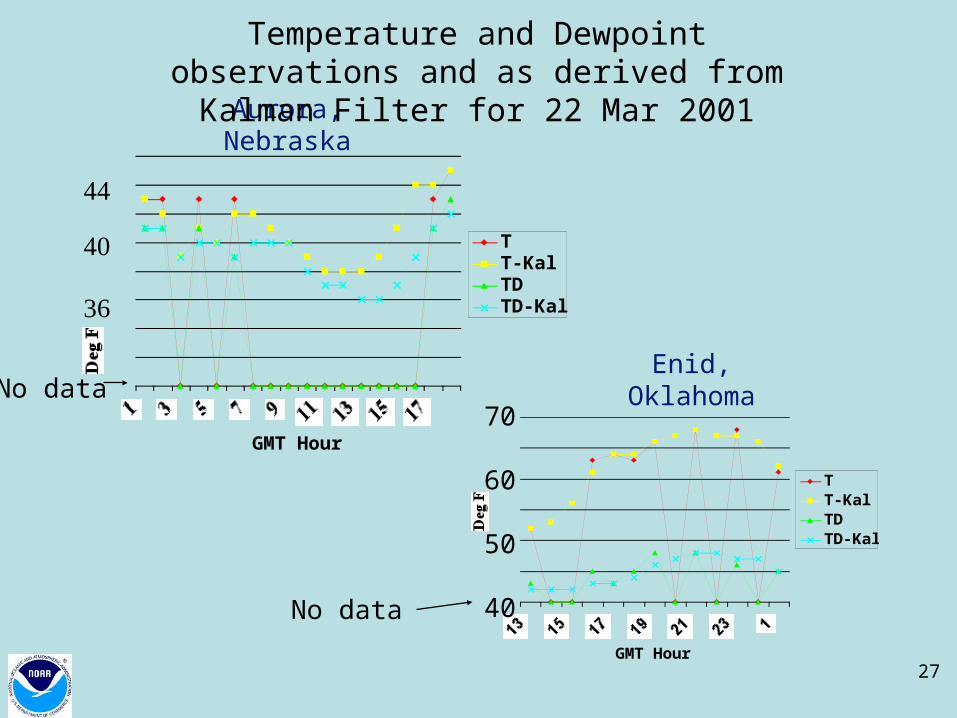
27

Aurora, Nebraska

1 3 5 7 9 11 13 15 17

GMT Hour

Deg F

TT-KalTDTD-Kal

0

3

No data

Temperature and Dewpoint observations and as derived from Kalman Filter for 22 Mar 2001

Enid, Oklahoma

13 15 17 19 21 23 1

GMT Hour

Deg F

TT-KalTDTD-Kal

70

60

50

40No data

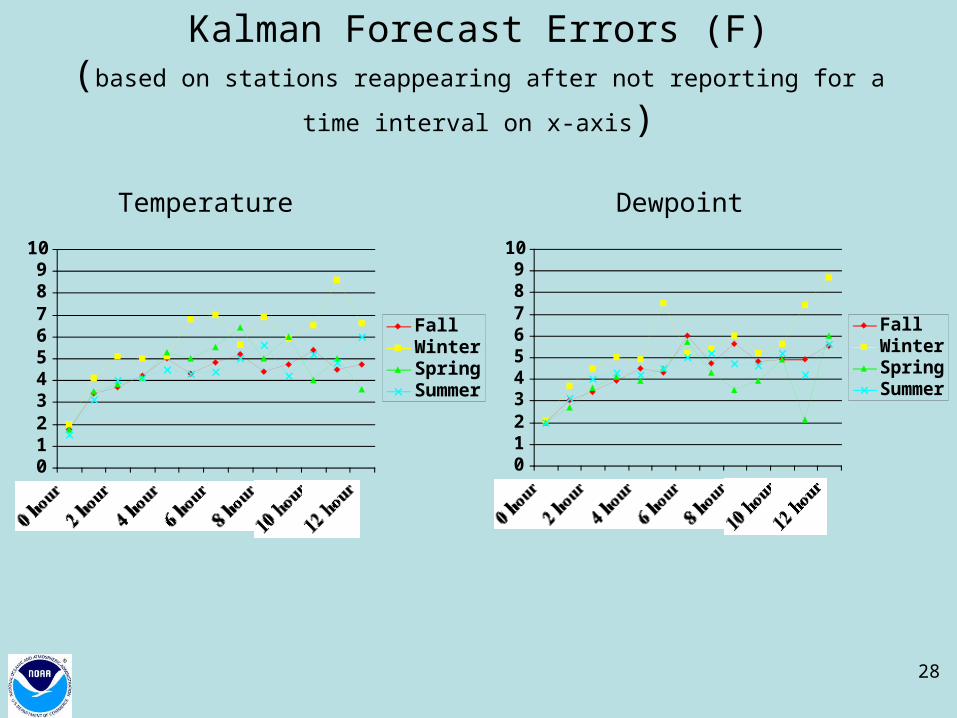
28

Kalman Forecast Errors (F)(based on stations reappearing after not reporting for a time interval on x-axis)

0123456789

10

0 hour2 hour4 hour6 hour8 hour10 hour12 hour

FallWinterSpringSummer

Temperature

0123456789

10

0 hour2 hour4 hour6 hour8 hour10 hour12 hour

FallWinterSpringSummer

Dewpoint

29

More about STMAS

• Ability to use background fields from a model (e.g., RUC) or a previous analysis (these features were adapted from LAPS and are important to have in the data-void desert regions)

• Background fields are modified to account for very detailed terrain (another useful feature borrowed from LAPS)

• Background field includes lake and sea surface temperatures and a land-weighting scheme to prevent situations such as warm land grid points having an influence on cooler water areas (via LAPS)

• Currently, STMAS compares observations to background for its QC method. Kalman filter will provide both a much more sophisticated QC and the ability to fully utilize temporal detail in the data.

• Reduced pressure calculation for a given reference height, as in LAPS (may see perturbation pressure sometime in the future)

• Value of STMAS is being measured relative to the LAPS analysis• Analyses currently conducted over CIWS domain every 15 minutes

on a 5-km grid (a variety of grid product fields are computed)

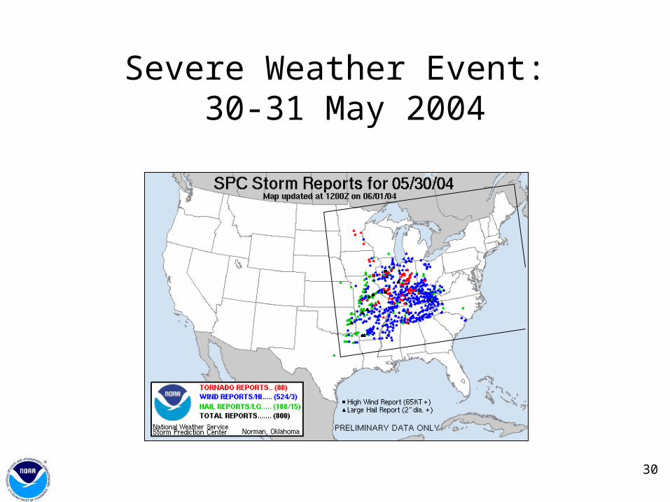
30

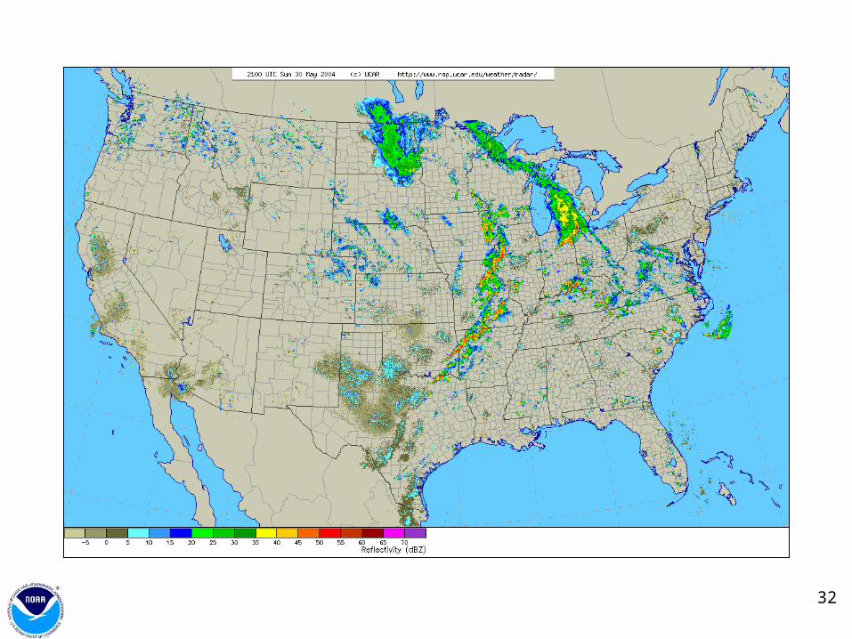
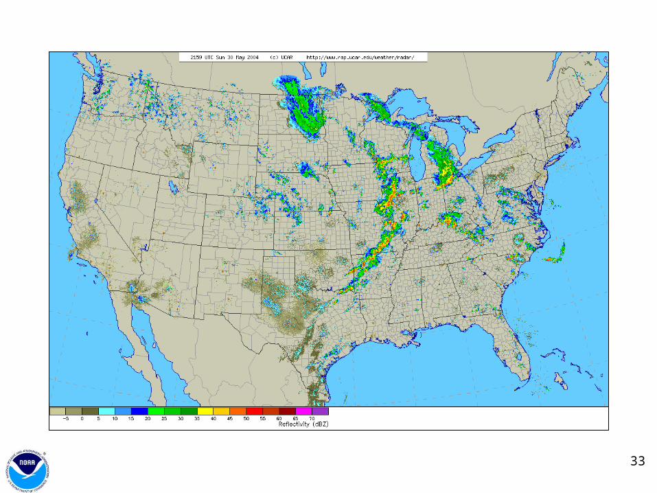
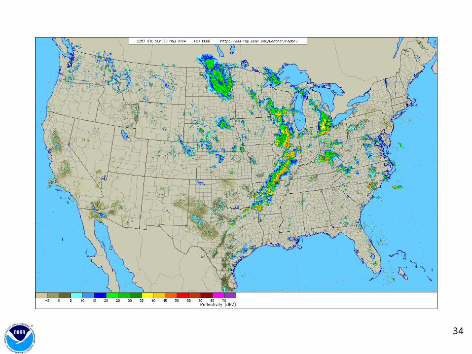
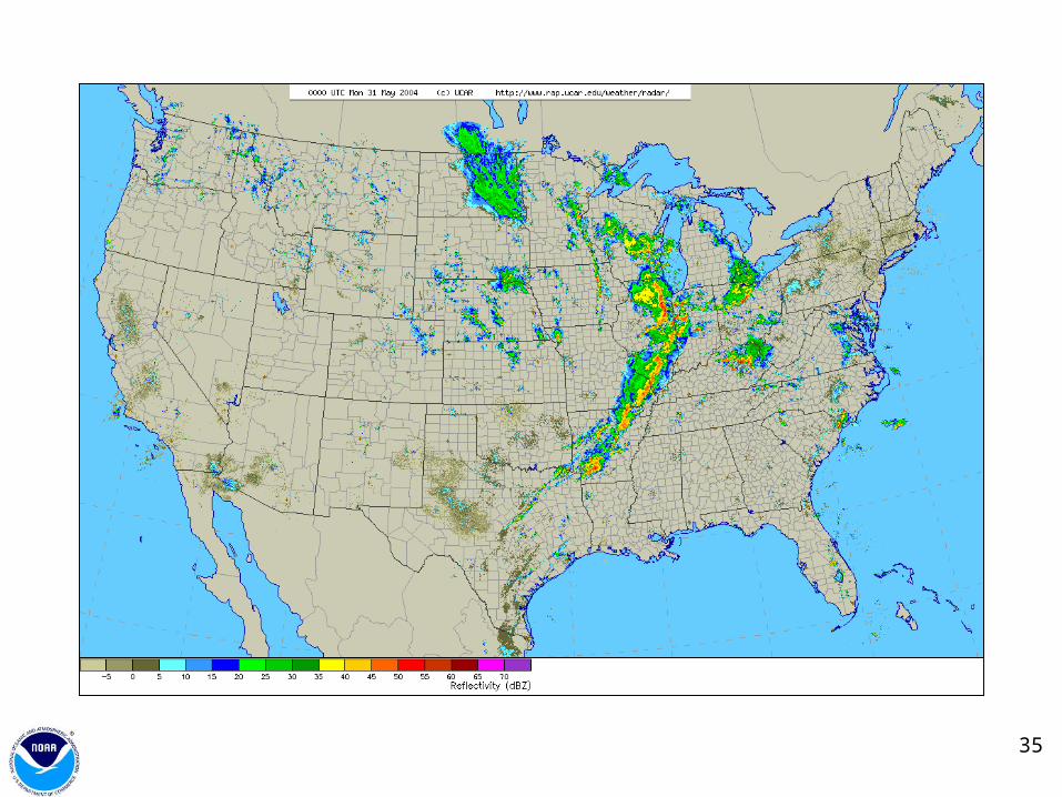
Severe Weather Event: 30-31 May 2004

31

2000 UTC

32

2100 UTC

33

2200 UTC

34

2300 UTC

35

0000 UTC

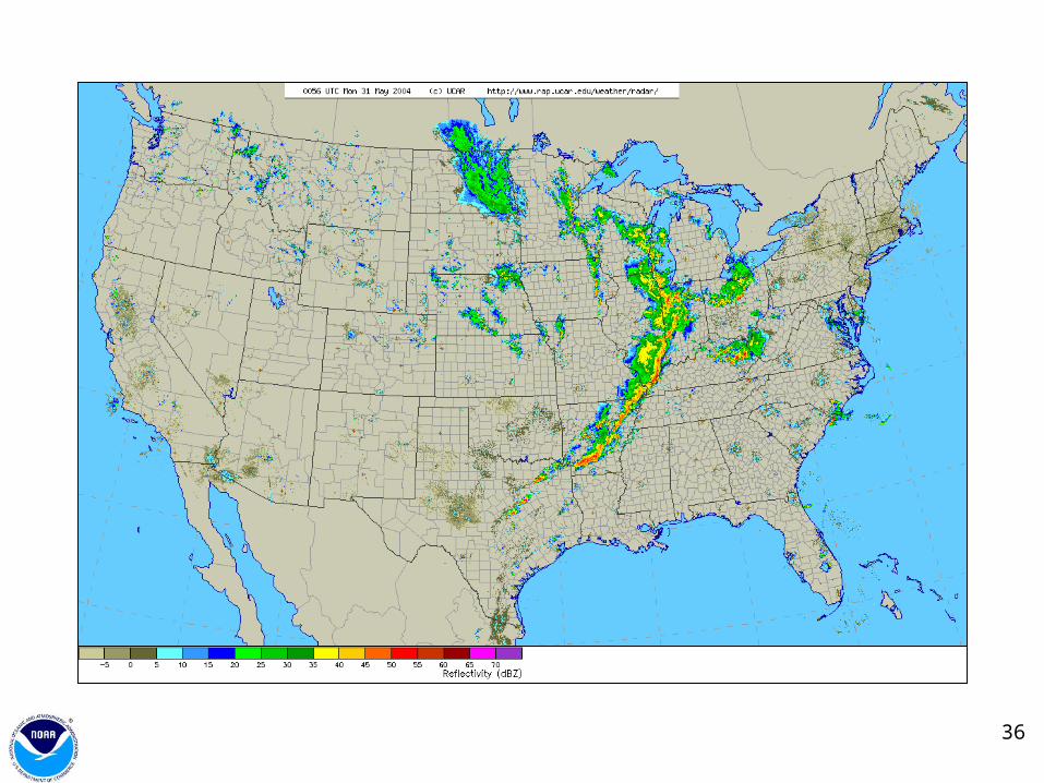
36

0100 UTC

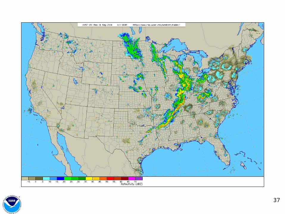
37

0200 UTC

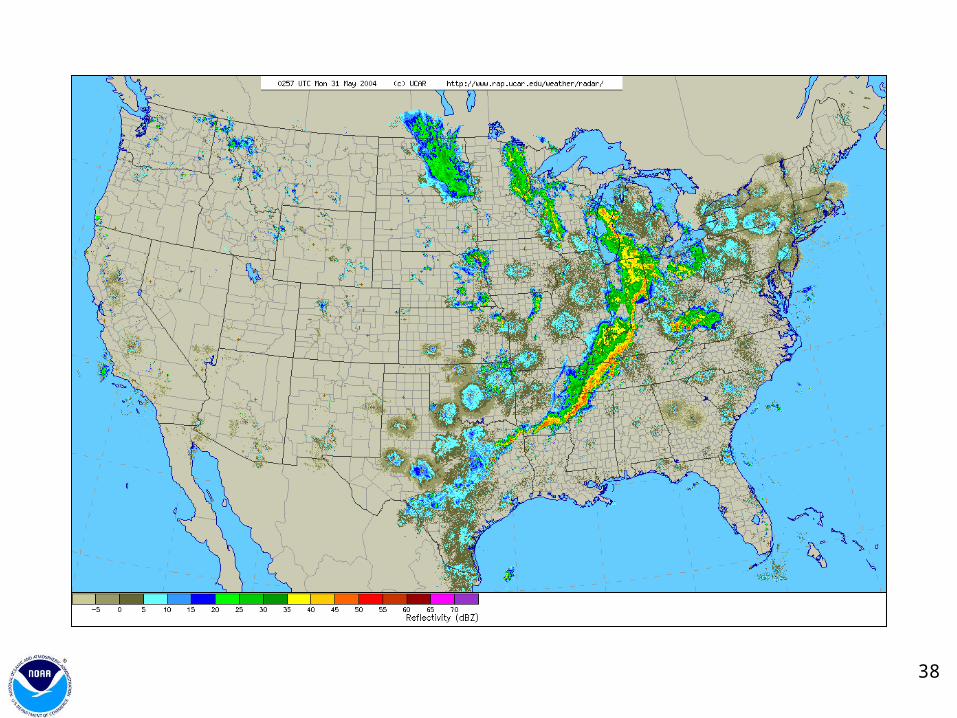
38

0300 UTC

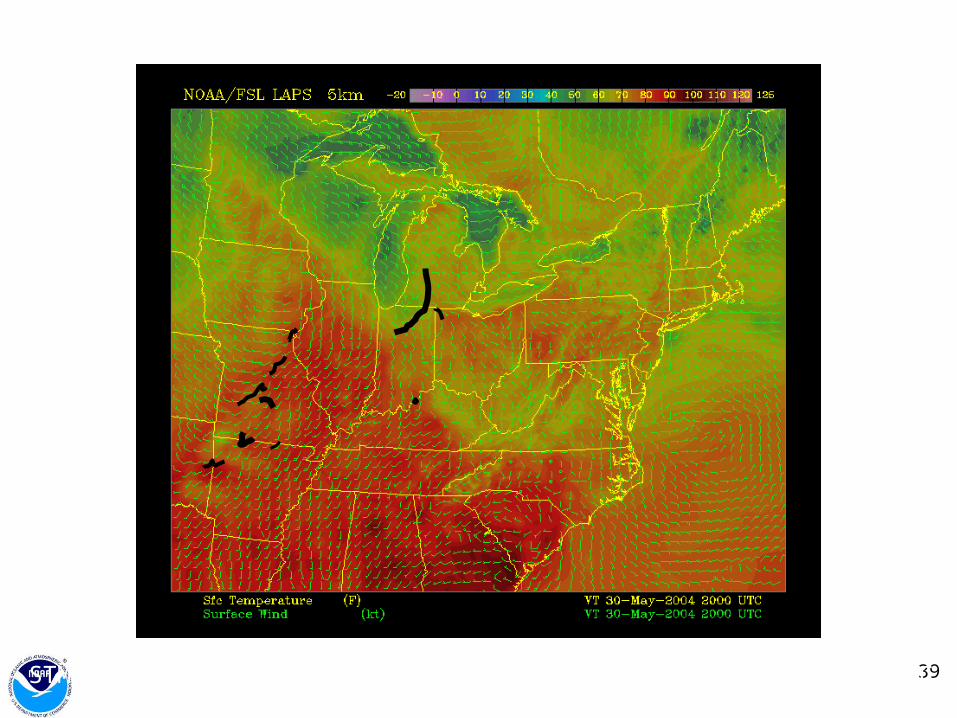
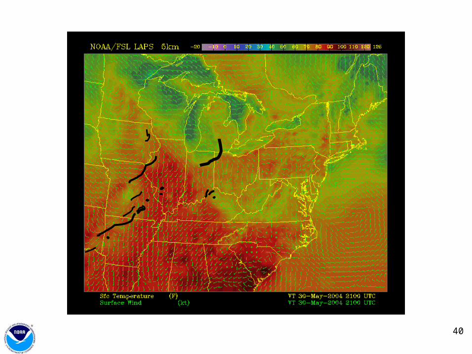
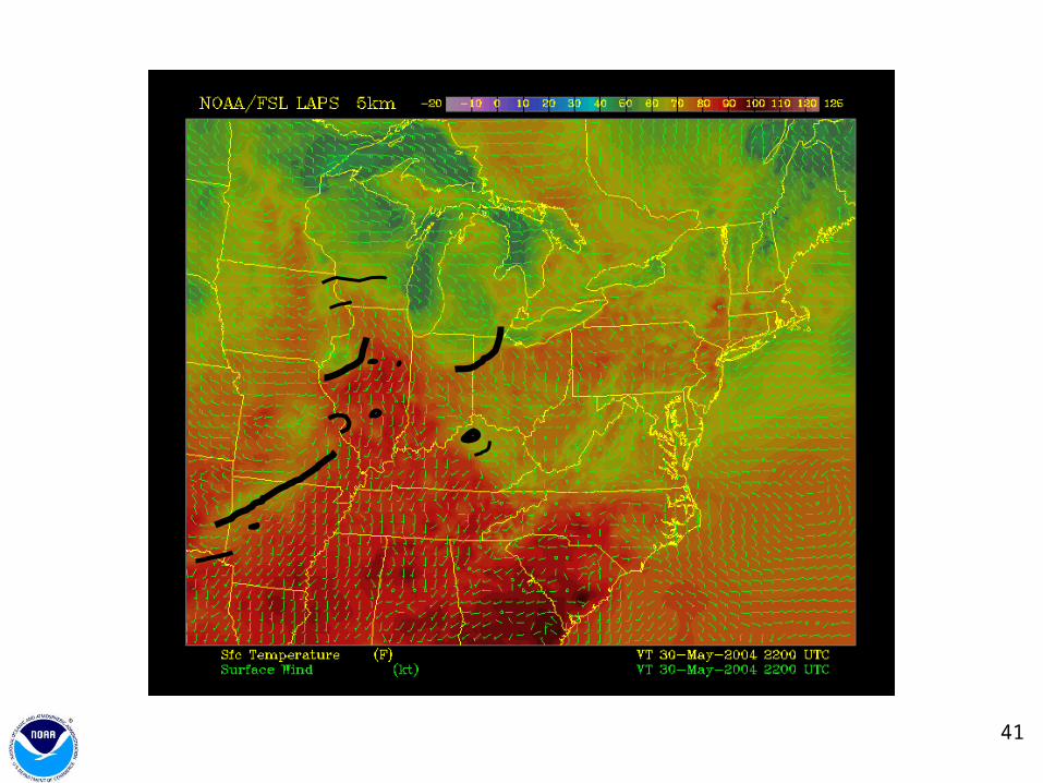
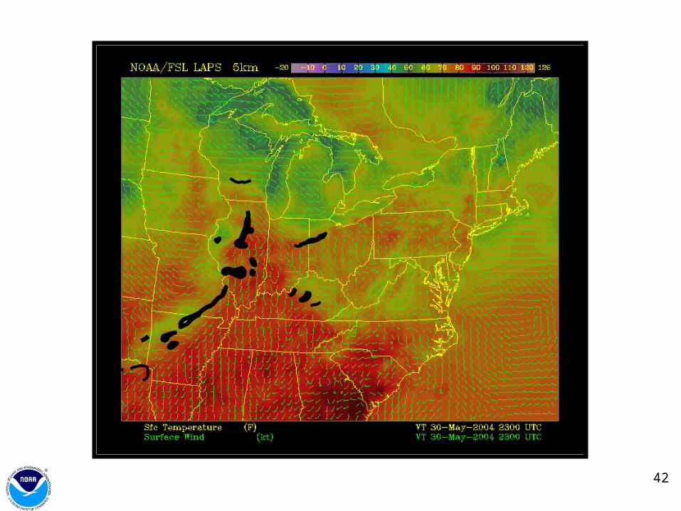
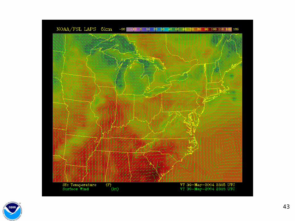
39STMAS analysis of temperature and winds: 20 UTC 30 May - 01 UTC 31 May 2004

2000 UTC

40

2100 UTC

41

2200 UTC

42

2300 UTC

43

0000 UTC

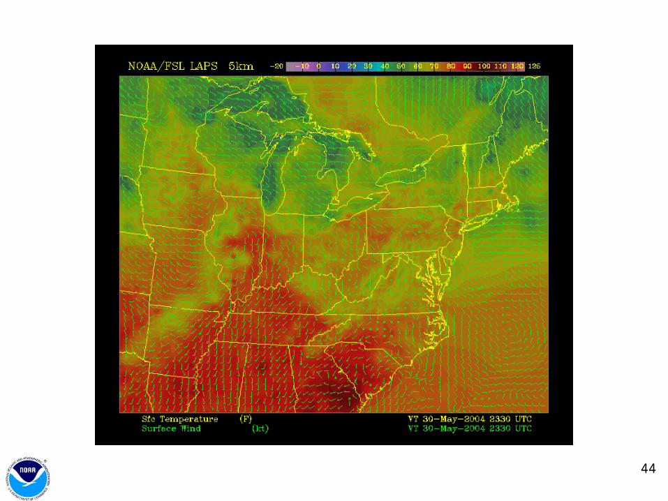
44

2330 UTC

45

2345 UTC

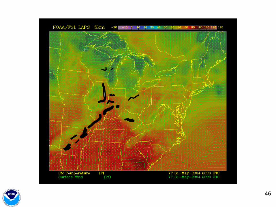
46

2315 UTC

47

0015 UTC

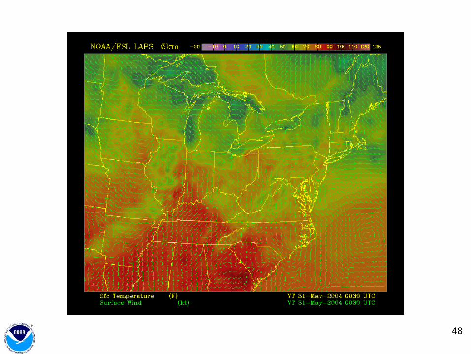
48

0030 UTC

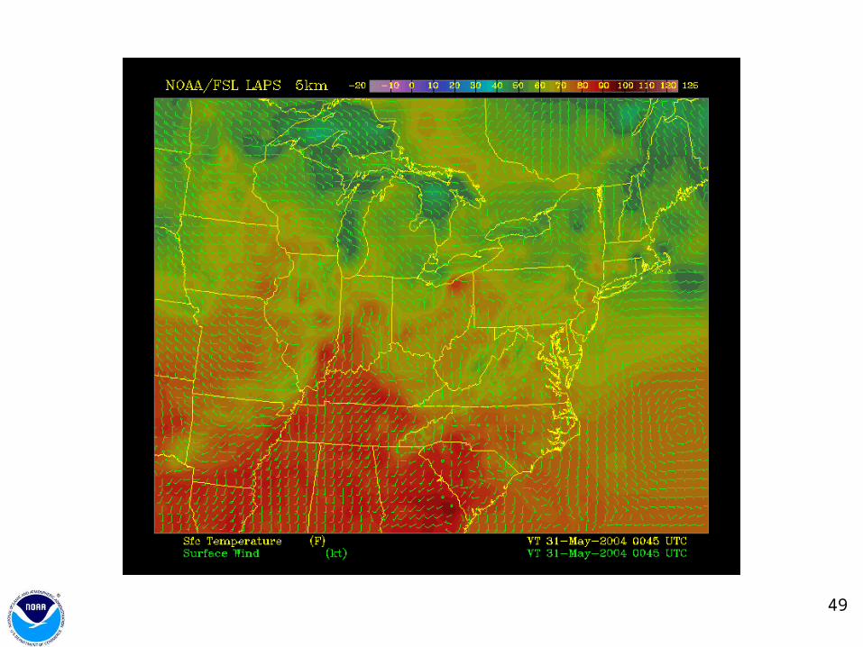
49

0045 UTC

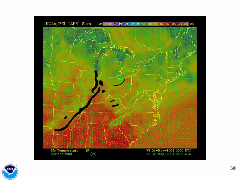
50

0100 UTC

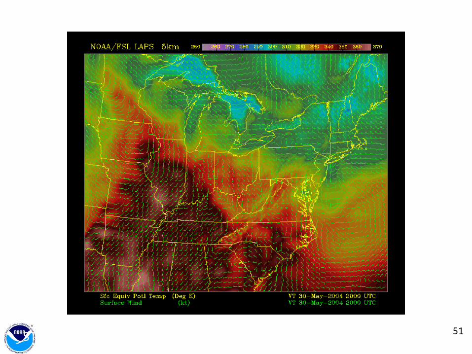
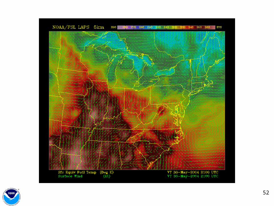
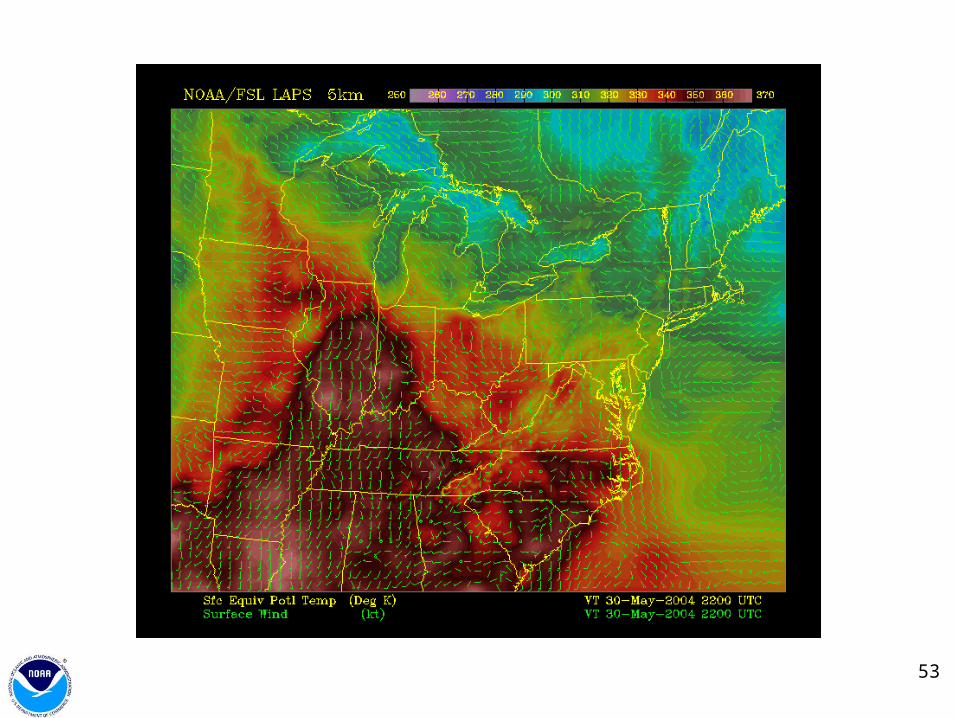
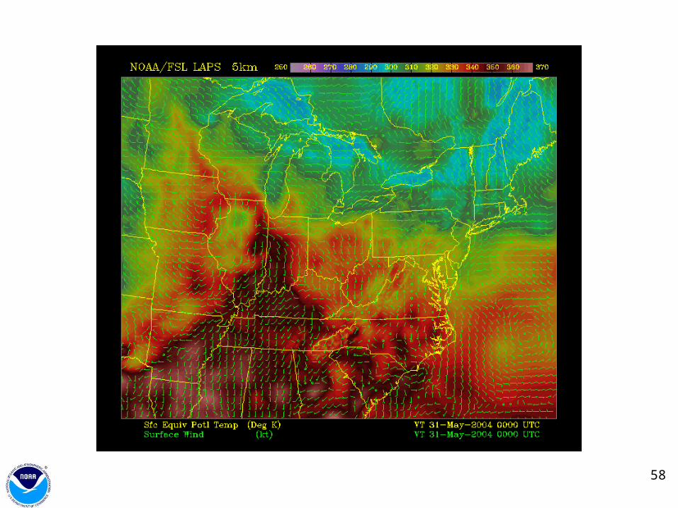
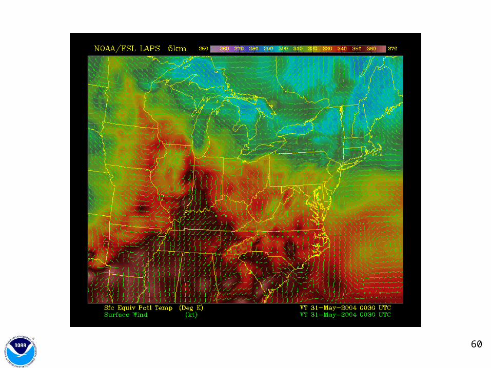
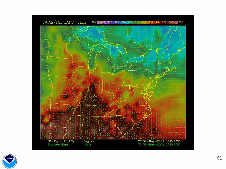
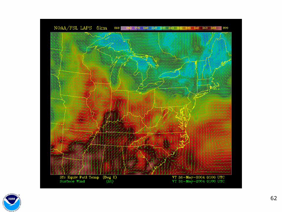
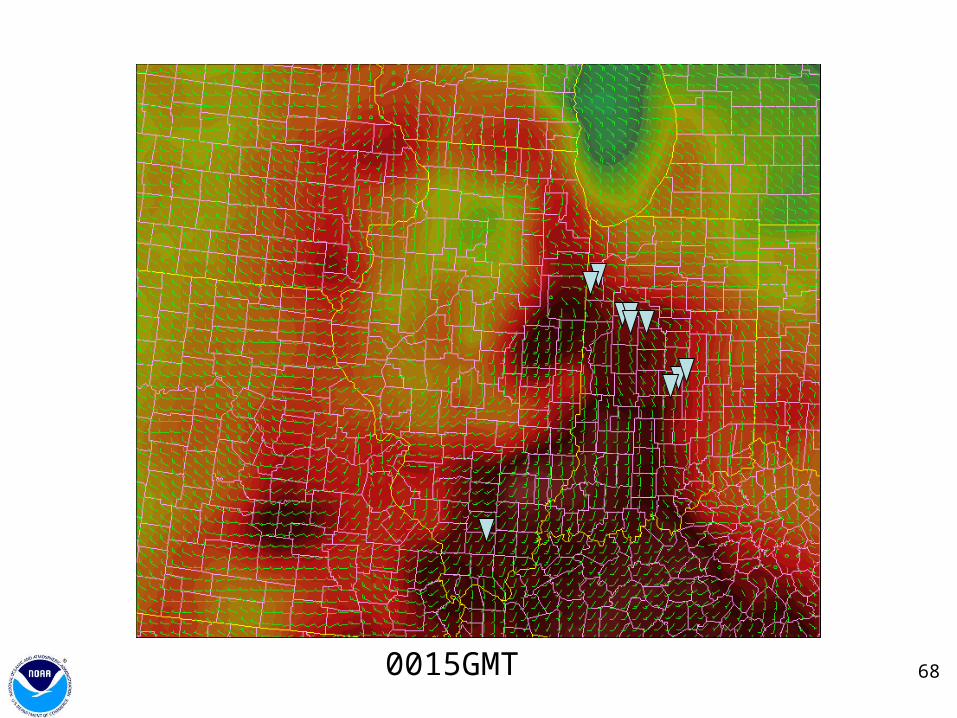
51STMAS analysis of equivalent potential temperature and winds

2000 UTC

52

2100 UTC

53

2200 UTC

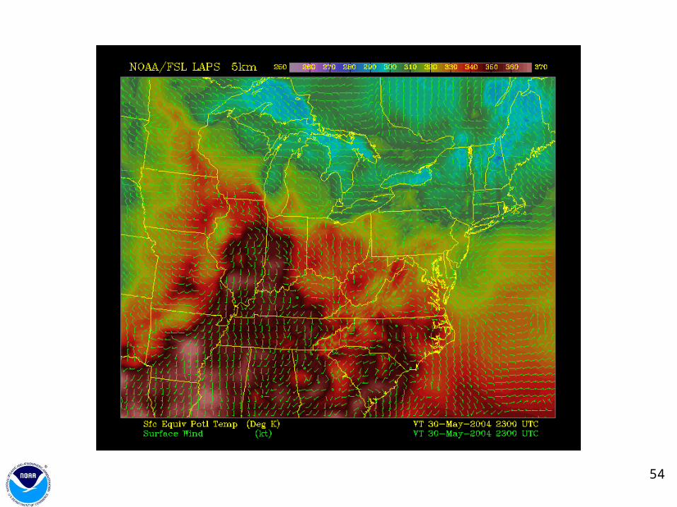
54

2300 UTC

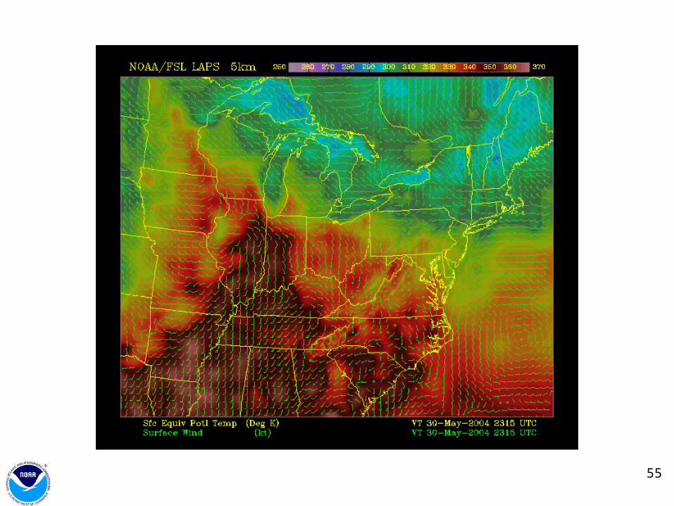
55

2315 UTC

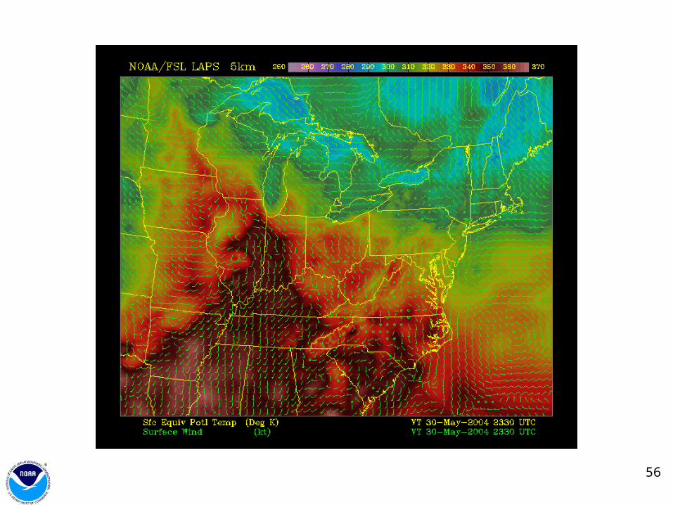
56

2330 UTC

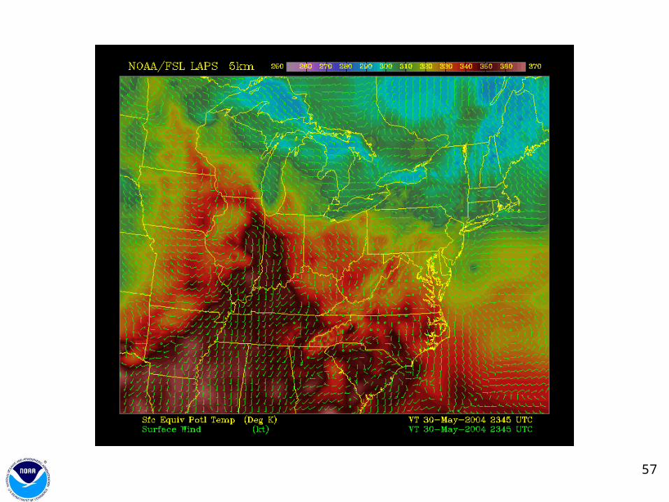
57

2345 UTC

58

0000 UTC

59

0015 UTC

60

0030 UTC

61

0045 UTC

62

0100 UTC

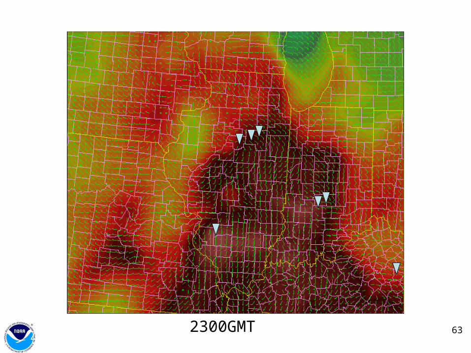
63

2300 UTC

Zoomed-in analysis of equivalent potential temperature and winds2300GMT

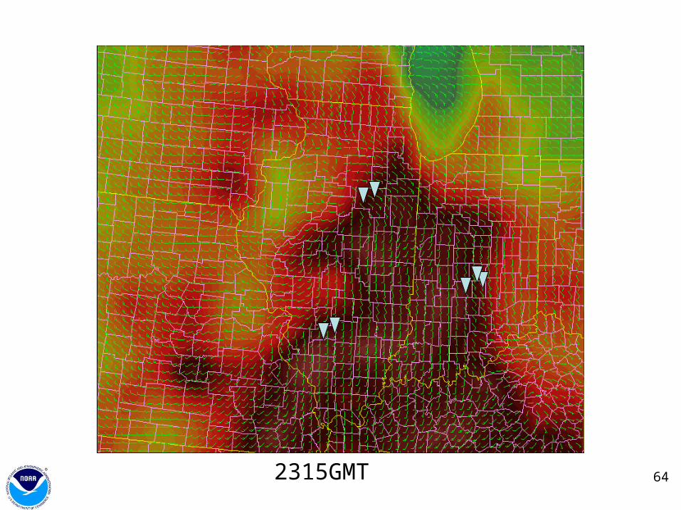
64

2315 UTC

2315GMT

65

2330 UTC

2330GMT

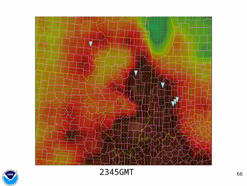
66

2345 UTC

2345GMT

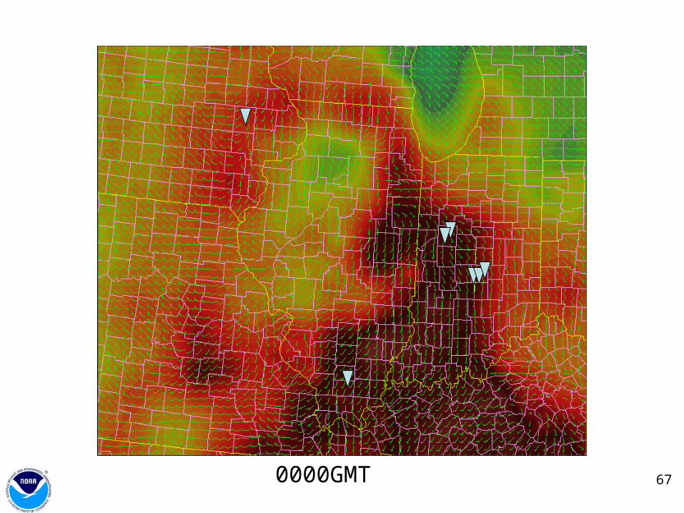
67

0000 UTC

0000GMT

68

0015 UTC

0015GMT

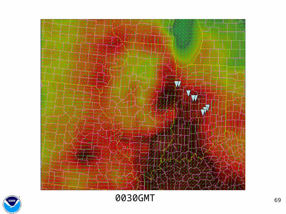
69

0030 UTC

0030GMT

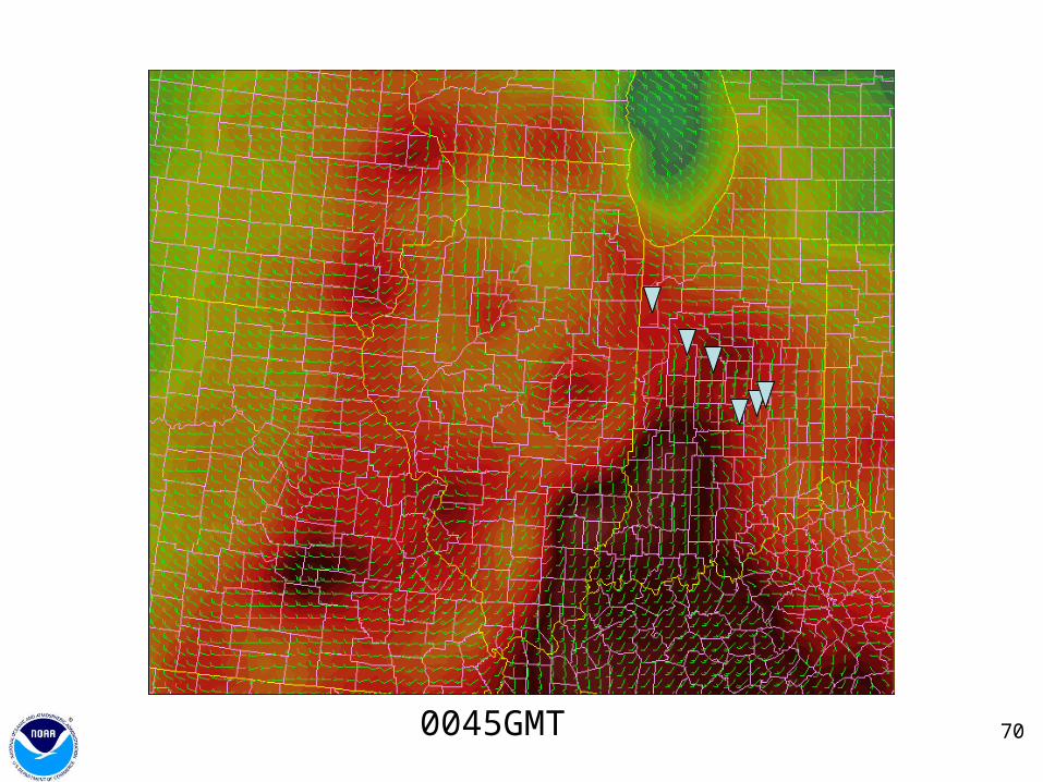
70

0045 UTC

0045GMT

71

0100 UTC

0100GMT

72

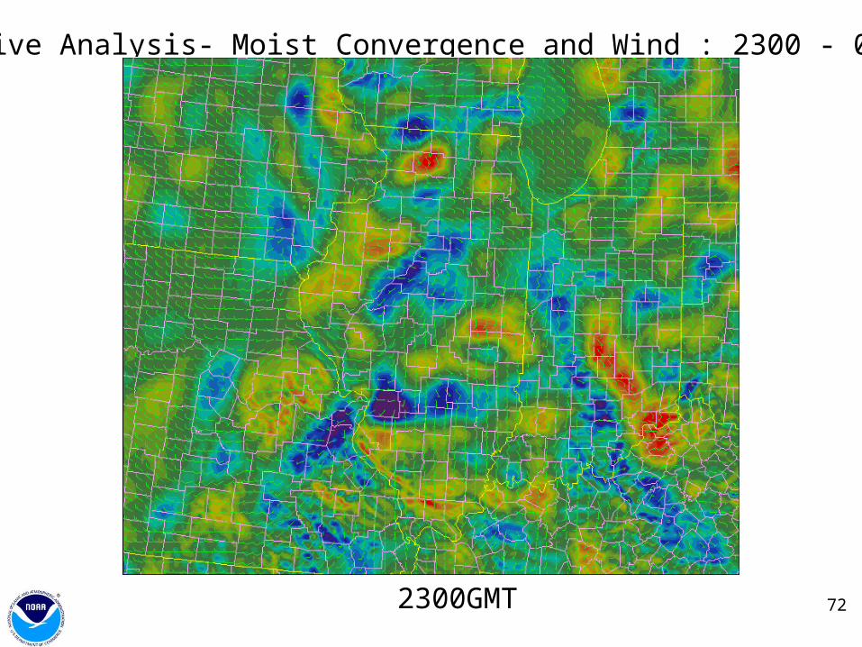
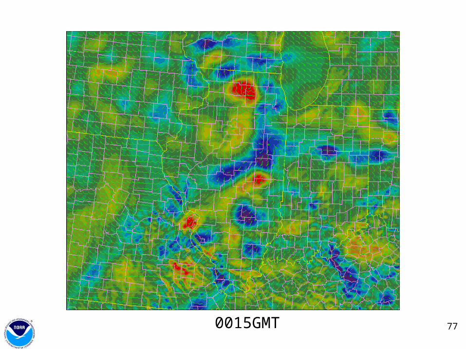
Recusive Analysis- Moist Convergence and Wind : 2300 - 0100

Zoomed-in analysis of moisture convergence2300GMT

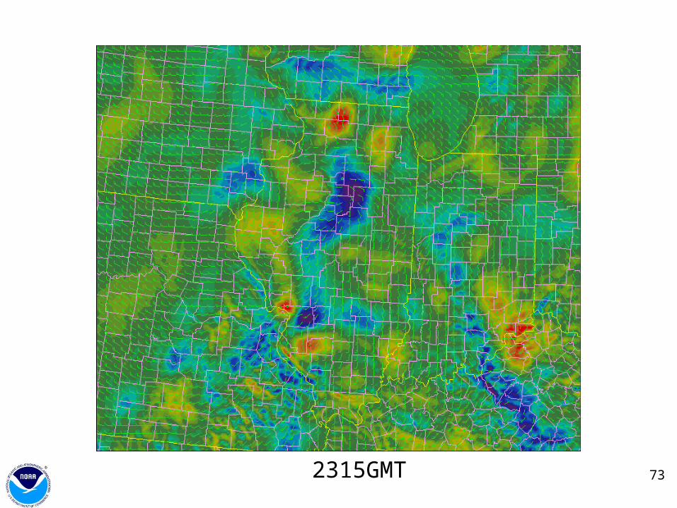
73

2315 UTC

2315GMT

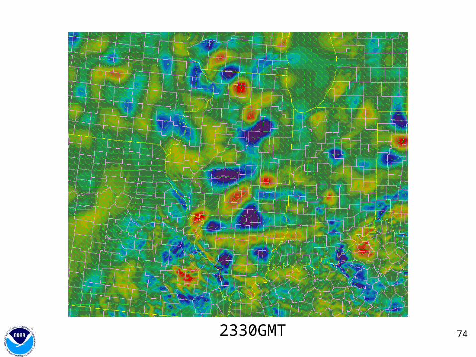
74

2330 UTC

2330GMT

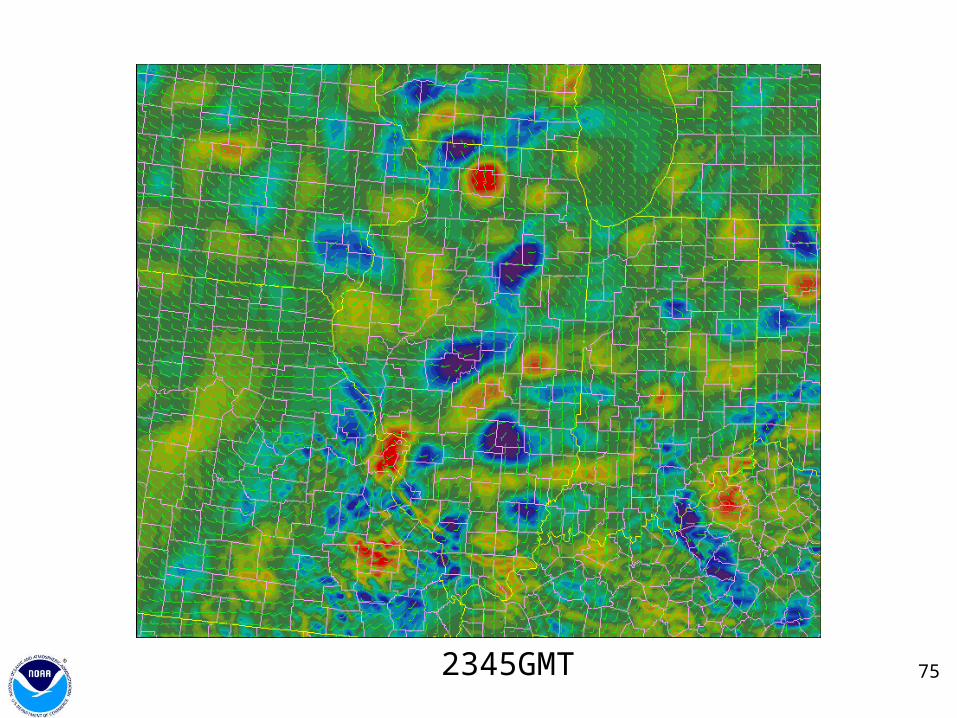
75

2345 UTC

2345GMT

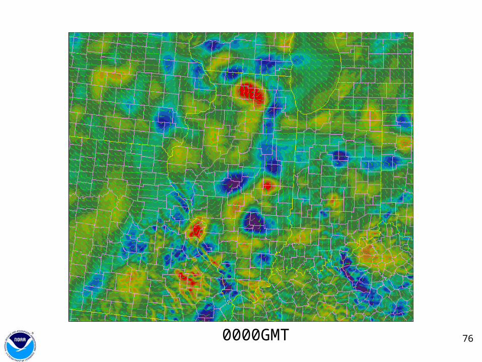
76

0000 UTC

0000GMT

77

0015 UTC

0015GMT

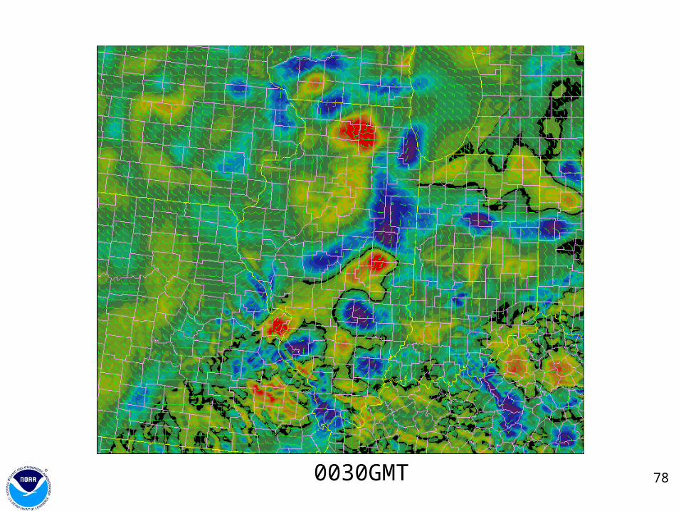
78

0030 UTC

0030GMT

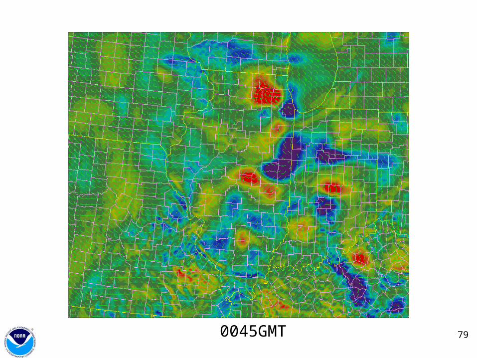
79

0045 UTC

0045GMT

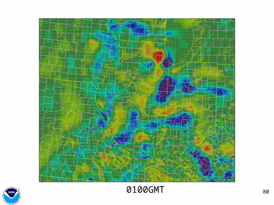
80

0100 UTC

0100GMT

81

Summary

• STMAS is capable of high time and space resolution of important parameters for mesoscale weather

• Shows good time continuity• Features correlate well with independent

observations such as radar• Need to enhance analysis with wavelet

scheme• Need to get robust Kalman QC into scheme

82

Future

• Ensure compatibility with AWIPS• Work in more model background options

(RUC and Eta)• Utilize STMAS fields for automated boundary

diagnostics• Work toward a spatial 3-D scheme

83

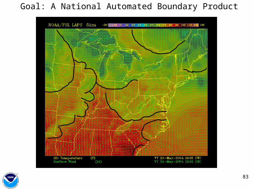
0015 UTCGoal: A National Automated Boundary Product

84

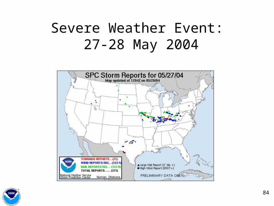
Severe Weather Event: 27-28 May 2004

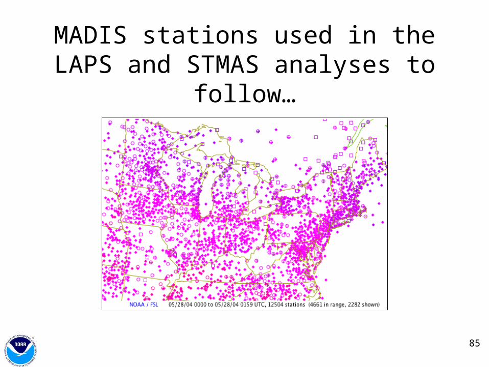
85

MADIS stations used in the LAPS and STMAS analyses to follow…

86

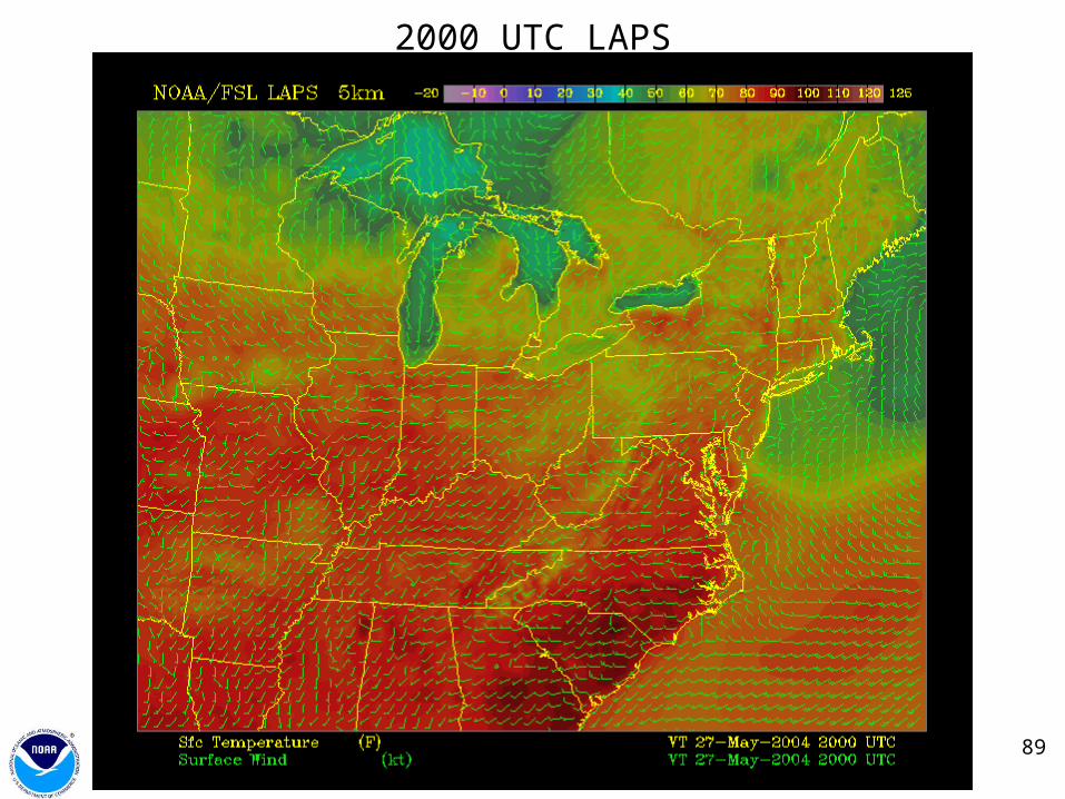
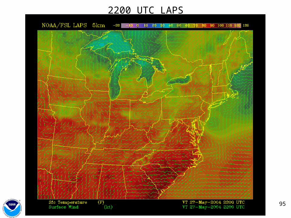
Comparisons of hourly analyses of temperature and winds using

LAPS and STMAS to surface and radar observations

Hourly analyses: 1900 - 2200 UTC

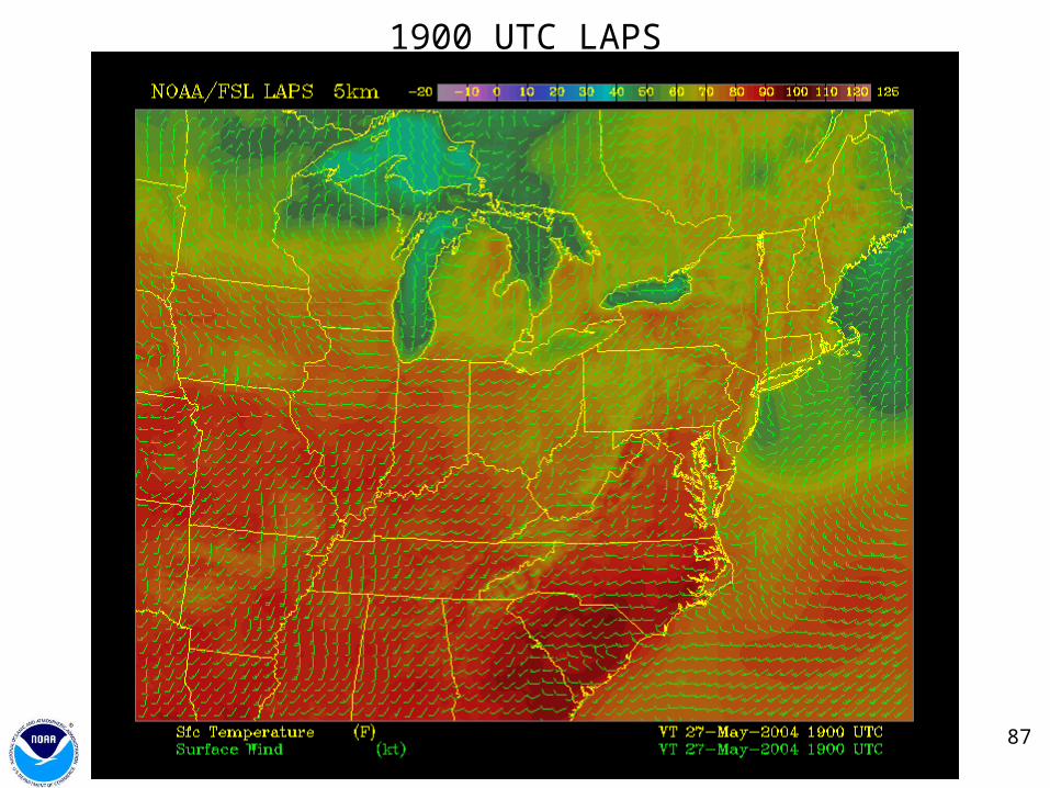
87

1900 UTC LAPS

88

1900 UTC STMAS

89

2000 UTC LAPS

90

2000 UTC STMAS

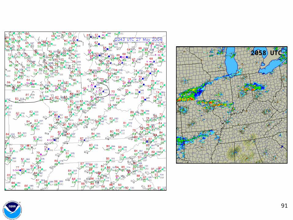
91

2058 UTC

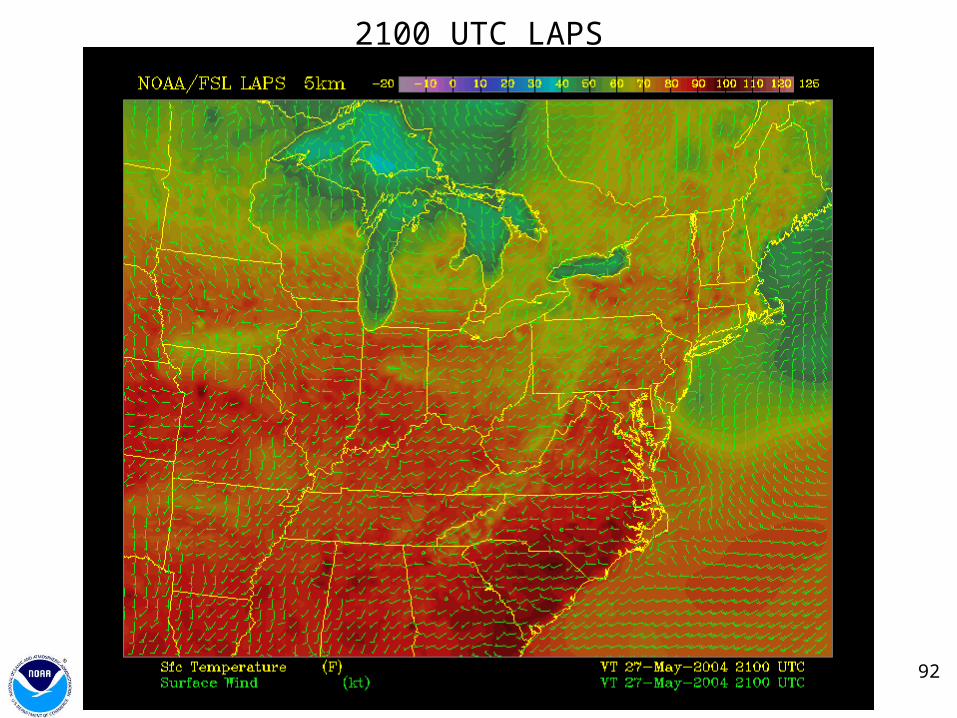
92

2100 UTC LAPS

93

2100 UTC STMAS

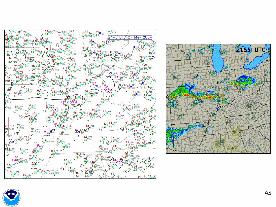
94

2155 UTC

95

2200 UTC LAPS

96

2200 UTC STMAS

97

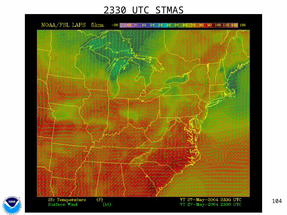
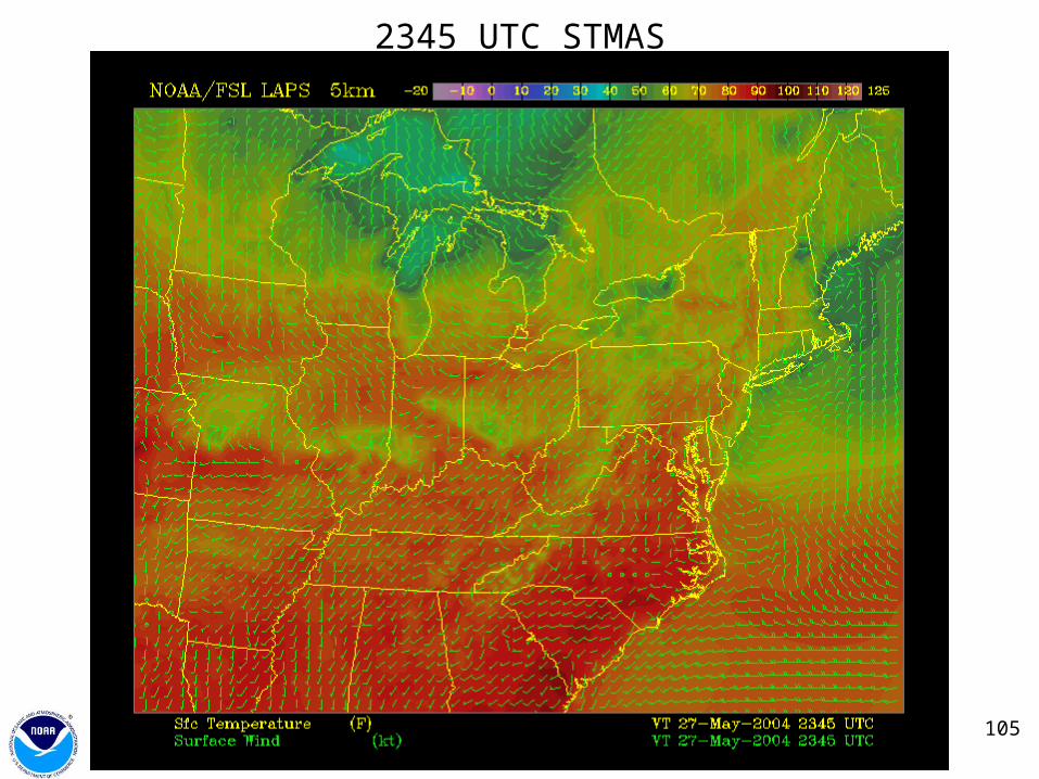
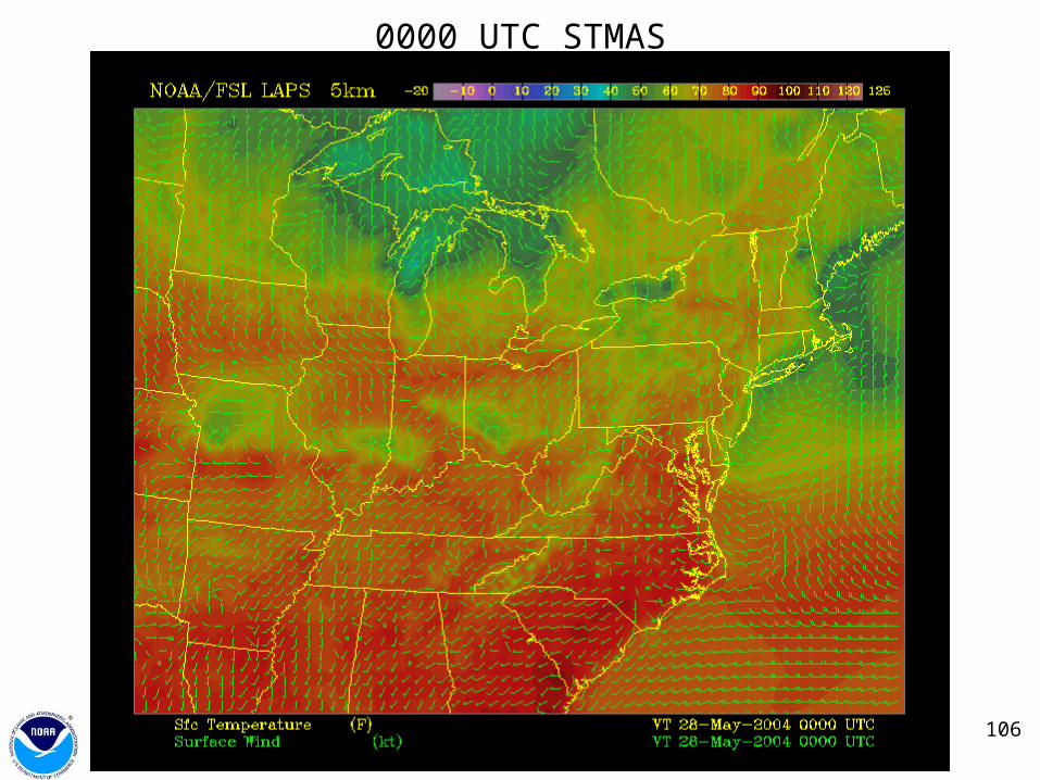
Analyses of Temperature and Winds using STMAS

15-min analyses: 2200 - 0000 UTC

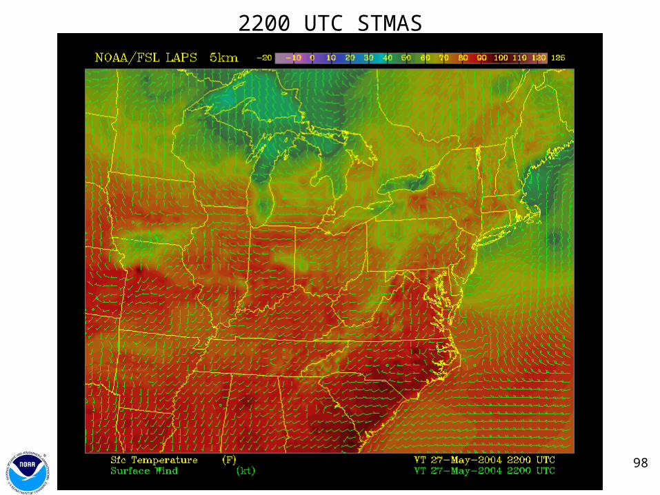
98

2200 UTC STMAS

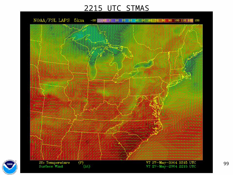
99

2215 UTC STMAS

100

2230 UTC STMAS

101

2245 UTC STMAS

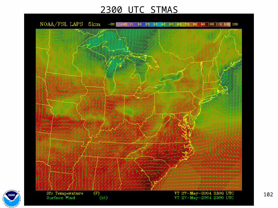
102

2300 UTC STMAS

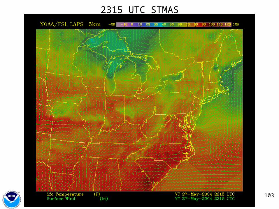
103

2315 UTC STMAS

104

2330 UTC STMAS

105

2345 UTC STMAS

106

0000 UTC STMAS

107

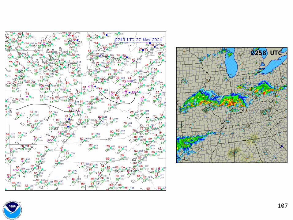
2258 UTC

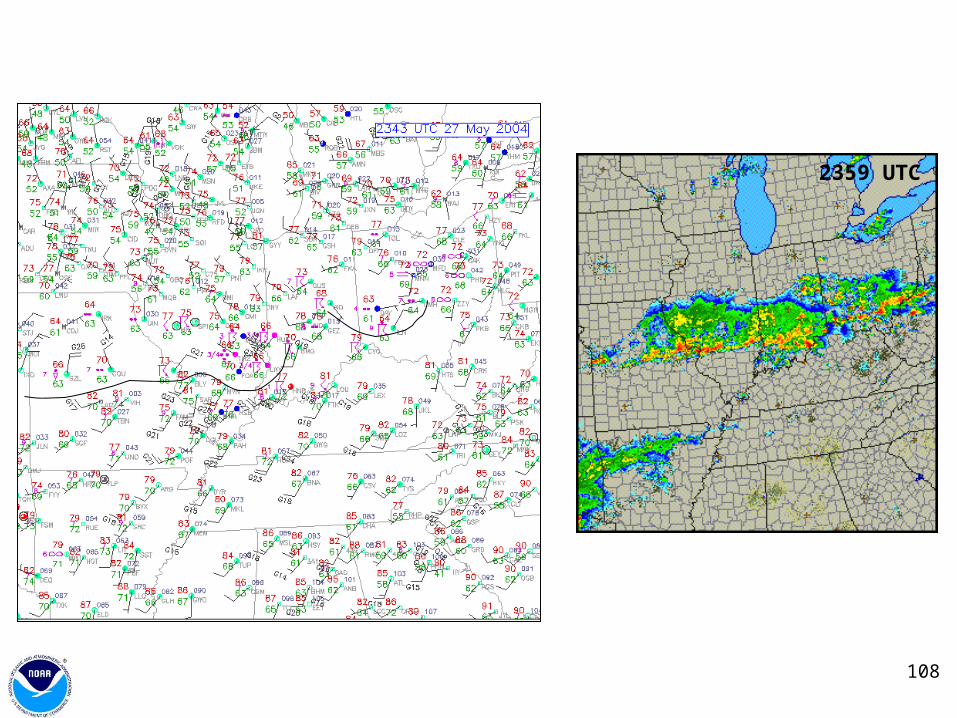
108

2359 UTC

109

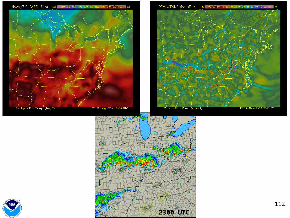
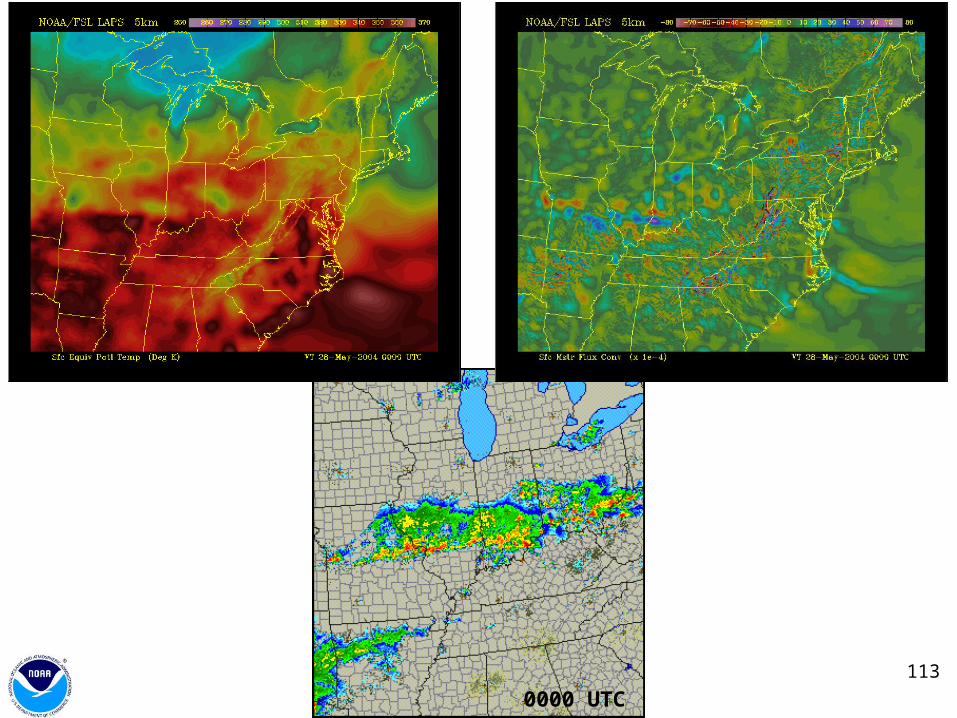
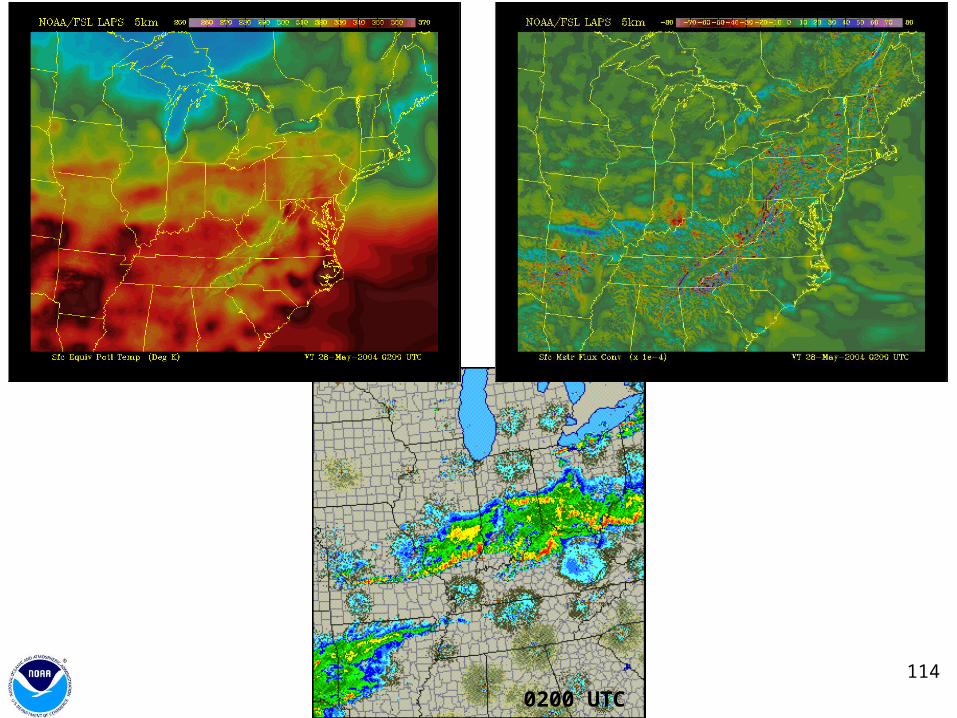
Relation of analyzed equivalent potential temperature and moisture convergence fields to radar echoes

2100 UTC 27 May - 0200 UTC 28 May

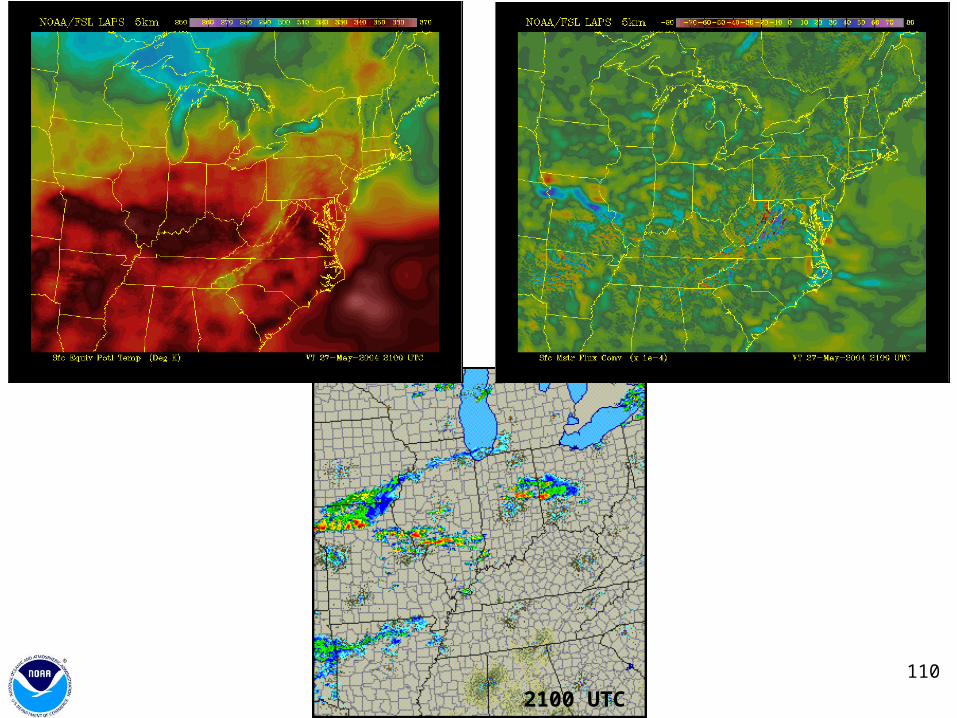
110

2100 UTC

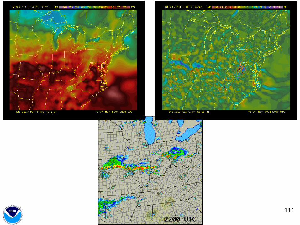
111

2200 UTC

112

2300 UTC

113

0000 UTC

114

0200 UTC

115

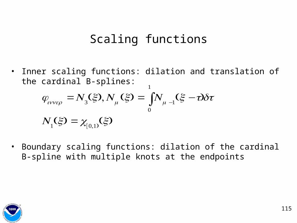
• Inner scaling functions: dilation and translation of the cardinal B-splines:

• Boundary scaling functions: dilation of the cardinal B-spline with multiple knots at the endpoints

Scaling functions

φinner

=N3(x),N

m(x) = N

m−10

1

∫ (x−t)dt

N1(x) =χ

[0,1)(x)

116

• Inner wavelet functions: dilation and translation of the cardinal B-wavelets:

• Boundary wavelet functions: dilation of the special B-wavelets derived from cardinal B-splines and boundary scaling functions

Wavelet functions

ψinner

= qn

n∑ N

m(2x−n),

qn=(−1)n

2m−1

ml

⎛

⎝⎜⎞

⎠⎟l=0

m

∑ N2m(n +1−l),n =0,..., 3m−2