1 Trey Porto Joint Quantum Institute NIST / University of Maryland LASSP Seminar Cornell Oct. 30 2007 Controlled exchange interactions between pairs of

1

Trey Porto Joint Quantum Institute

NIST / University of Maryland

LASSP SeminarCornell

Oct. 30 2007

Controlled exchange interactions between pairs of atoms in an

optical lattice

•Quantum information processingw/ neutral atoms

•Correlated many-body physicsw/ neutral atoms

•Engineering new optical trapping and control techniques

Research Directions

This Talk

Sub-lattice RF addressing in a lattice-independent Bloch-sphere control of atoms in sub-lattices

Controlled exchange-mediated interactions-using exchange to get spin-dependent entangling (SWAP)

Outline

-Description of the lattice

- Demonstrations of toolsdouble well splitting, controlled

motion, sub-lattice spin addressing

-Putting it all together:controlled two-atom exchange

swapping

Outline





swapping

Motivation for the double-well lattice:Isolate pairs of atoms in controllable potential, to test

- demonstrate addressing ideas - controlled interactions, at 2-

atom level

Provide new possibilities for cold atom

lattice physics

Double-Well Lattice

Phase Stable 2D Double Well

‘’ ‘’

Basic idea:Combine two different period lattices with adjustable

- intensities - positions

Mott insulator single atom/site

+ = A B

rε =y

+

=

/2

rε =z

nodes

16E2 sin4 kx / 2( )

4E2 cos2 kx +φ( ) +1( )

BEC

Mirror

z

y

x

Folded retro-reflection is phase stable

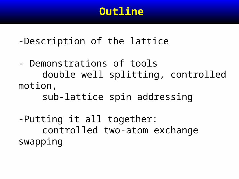
Polarization Controlled 2-period Lattice

Sebby-Strabley et al., PRA 73 033605 (2006)

Add an independent, deep vertical lattice

Provides an independent array of 2D systems

Polarization Controlled 2-period Lattice

Light Shifts

Scalar

Vector

∝ I

e

hg

Ω2 ~I

Intensity and state

dependent light shift

δU

Pure scalar, Intensity lattice

Intensity + polarization

Effective B field, with -scale spatial structure

Flexibility to tune scalar vs. vector component

mF

€

rμ ⋅

rB

Red detuning attractiveBlue detuningrepulsive

Optical standing wave

Vector Light Shifts

x

y z

rε =x

rε =x

Example: lin || lin

no elipticity, intensity modulation

rε =x

rε =y

Example: lin lin⊥

no intensity modulation, alternating circular polarization

rBeff

Position dependent effective magnetic field

F =1,mF =0

F =1,mF =−1

F =1,mF =1

Vector light shift + bias B-field:controllable

state-dependent barriersstate-dependent tilts

Use for site-dependent RF addressing

State Dependent Potential

For the demonstrations

shown here, we use these 2 states in

87Rb

We use the quadratic Zeeman shift

to isolate a pseudo spin-1/2

~34 MHz

~34.3 MHz

~50 gauss

X-Y directions coupled- Checkerboard topology- Not sinusoidal (in all directions)

e.g., leads to very different tunneling- spin-dependence in sub-lattice- blue-detuned lattice is different- interesting Band-structure

Lattice Features

cos2 (x + y)cos (x−y) cos4 (x)

Outline





swapping

q

E

x

Lattice can be turned on/off in different time scales

Sudden: (<< 100 μs) (“pulsing” lattice)

Eigenstate projection

Intermediate:Fast compared to interaction/tunneling,Slow compared to non-interacting band

“Map” band distribution

Slow compared to all times: (>> few ms)

complete adiabaticity(“adiabatic”)

Dynamic Lattice Amplitude Control

Time of flight imaging

py

px

Reciprocal Lattices and Brillouin Zones

‘’ lattice ‘/2’ lattice

Band-adiabatic load in 500μs, snap off

300 ms500 μs

Brillouin Zone mapping

phase incoherent

500 μs 20 μs

Double Slit Diffraction

Slowly load mostly- lattice, snap off

Coherently split single well

Single slit diffraction

load in ~300 msphase scrambled

QuickTime™ and aAnimation decompressor

are needed to see this picture.



split in ~200 μscoherent split

Double slit diffraction

Time dependence of diffractiontime

Load and hold

Time dependence of diffraction

time

Contrast collapse:Not factorizable into a product state

LL + LR + RL + RR

L + R( ) L + R( ) =

e−iUt LL + LR + RL + e−iUt RR

split

++


time

No interaction, no collapse

L + R

split

+


time

N > 1

N =1

0.0 0.2 0.4 0.6 0.8 1.0 1.2 Time (ms)

In 3D lattice, see:Greiner et al.Nature, 419 (2002)

Sebby-strabley, PRL 98, 200405 (2007)

Loading (Slowly) One Atom Per Site

Step 1: (for most experiments)

Start with a Bose-Einstein condensate,slowly turn on the lattice

Load one atom per site using the Mott-Insulator transition

or

Well “fermionized”, but some holes

Probe: Selective Removal of Sites

Load right well expel left

Load left well expel left

band map

band map





“Expelling” as a left/right probe

dump left

dump left

dump left

“Expelling” as a left/right probe

Scan the relative phase between lattices

Relative phase =0



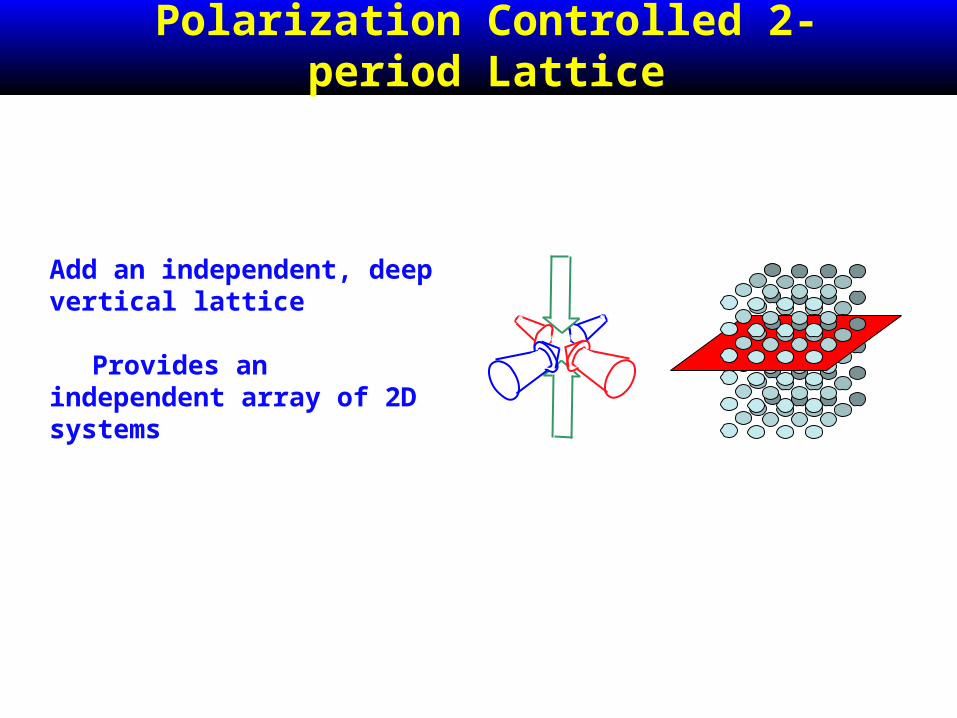
~ ms transfer time

atoms can be put on the same site, (but different vibrational level), allowed to interact, and then separated adiabatically

mapped at t0

from ‘’ lattice mapped at tf

from ‘/2’ lattice

Adiabatic transfer “excitation”

F =1,mF =0

F =1,mF =−1

State Dependent Potential

34 MHzZeeman

~150 kHzLattice

Start with atoms in m=-1

Apply RF to spin flip to m=0

“Evaporate” m=0 atoms

Measure m=-1 occupation in the left or right well.

sub-lattice addressing by light shift gradient

Sub-Lattice Addressing

1.0

0.8

0.6

0.4

0.2

0.0

P1 /(P

1+P

2)

34.3134.3034.2934.2834.2734.2634.25

freq_(MHz)_0063_0088

Right Well Left Well

RF RF

Left sites

Right sites

Start with atoms in m=-1

Apply RF to spin flip to m=0

“Evaporate” m=0 atoms

Measure m=-1 occupation in the left or right well.

1.0

0.8

0.6

0.4

0.2

0.0

P1 /(P

1+P

2)

34.3134.3034.2934.2834.2734.2634.25

freq_(MHz)_0063_0088

Right Well Left Well

Sub-Lattice Addressing

Right well

Left well

Lee et al., PRL 99, 020402 (2007)

Atoms at sub- spacing-focused beam sees

several sites

Example: Addressable One-qubit gates



several sites

- state dependent shifts

effective field gradients



several sites



RF, μwave or Raman



several sites



- frequency addressing

State selective motion/splitting

Start with either m=-1 or m=0Selectively and coherently

split wavefunction

m=0 on left m=-1 on right

or

Outline





swapping

Putting it all together: a swap gate

Step 1: load single atoms into sites

Step 2: spin flip atoms on right

Step 3: combine wells into same site

Step 4: wait for time T

Step 5: measure state occupation(vibrational + internal)

1)

2)

3)

4)



Exchange Gate:

0,1 + 1,0

00

1,1

0,1 −1,0

0,1

1,0

exchange split by energy U

0,0

1,1

projection1,0

swap

projection triplet

singlet

Exchange Gate:

0,1 + 1,0

00

1,1

0,1 −1,0

0,1

1,0


0,0

1,1

projection1,0

swap

projection triplet

singlet

r1 = r2r1 = r2

€

U ≅ 0

€

U ≠ 0

Exchange Gate:

0,1 + 1,0

00

1,1

0,1 −1,0

0,1

1,0


0,0

1,1

projection1,0

projection triplet

singlet

0,1 + i 1,0

0,1 −i 1,0

0,0

1,1

swap0,1 −i 1,0

swap

T−1 = ↓↓

T1 = ↑↑

T0 = ↑↓ + ↓↑

S = ↑↓ −↓↑

Controlled Exchange Interactions

Basis Measurements

Stern-Gerlach + “Band-mapping”

Swap Oscillations

Onsite exchange -> fast140μs swap time ~700μs total manipulation time

Population coherence preserved for >10 ms.( despite 150μs T2*! )

Anderlini, Nature 448 452 (2007)

Coherent Evolution

First /2 Second /2

RF RF

- Initial Mott state preparatio(30% holes -> 50% bad pairs)

- Imperfect vibrational motion~85%

- Imperfect projection onto T0, S ~95%

- Sub-lattice spin control >95%

- Field stabilitymove to clock states

(state-dependent control through intermediate states)

Current (Improvable) Limitations

Coherent collisional gatesNeighboring atoms are

-spatially isolated

or-in “activated”

states

Example: Two-qubit control

Optical tweezer adiabatically brings neighboring atoms together.

Coherent collisional shift


-spatially isolated


states


Optical tweezer adiabatically brings neighboring atoms together.

Atoms are separated after an interaction time.

Coherent collisional shift


-spatially isolated


states


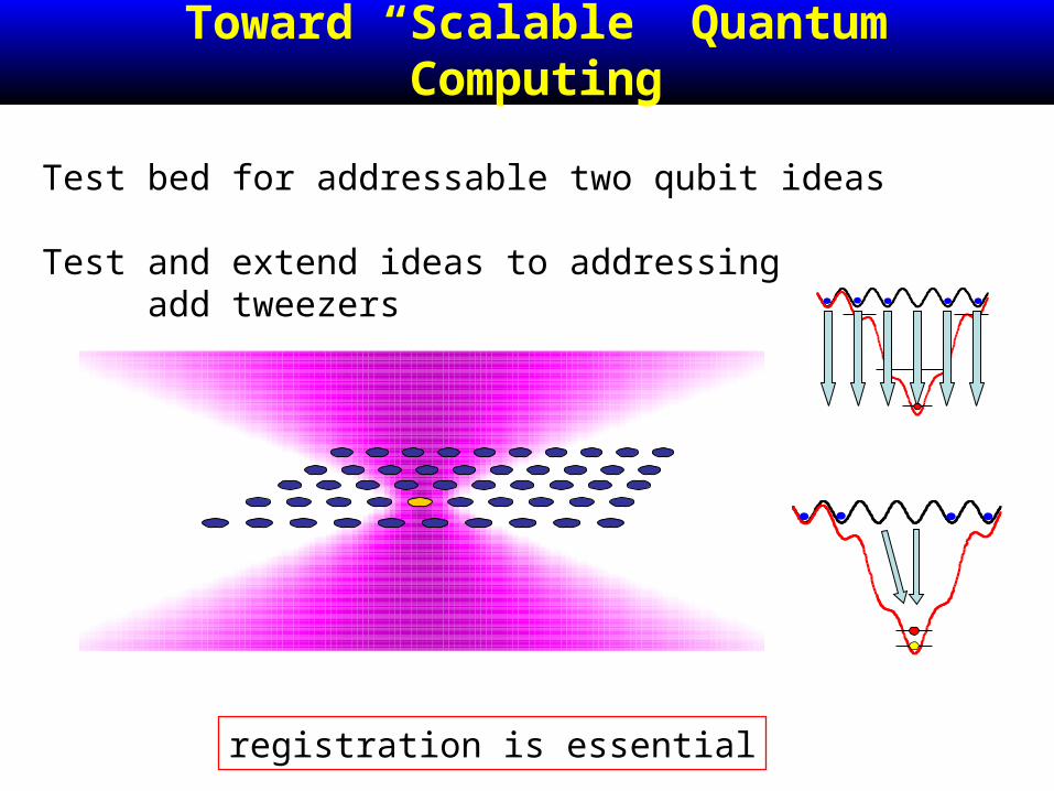
Toward “Scalable” Quantum Computing

Test bed for addressable two qubit ideas

Test and extend ideas to addressingadd tweezers

registration is essential

Using Parallelism

Quantum Cellular Automatalimited addressability (e.g. on the edges)distinct entangling, nearest neighbor rules

Formally equivalent to circuit Qcomp

Individually address only the edge atoms

B-rulesA-rules

Using Parallelism

Measurement Based or“One way” or “Cluster State” Qcomp

-Create a parallel-entangled cluster state-measurements + 1-qubit rotations

Entangled with each of its neighbors

Tools for lattice systems

State preparation, e.g.- ‘filter’ cooling- constructing anti-ferromagnetic

state.

Diagnostics, e.g.- number distributions (including

holes)- neighboring spin correlations

Realizing lattice Hamiltonians, e.g.- band structure engineering- ‘stroboscopic’ techniques- coupled 1D-lattice “ladder”

systems- RVB physics

. . .

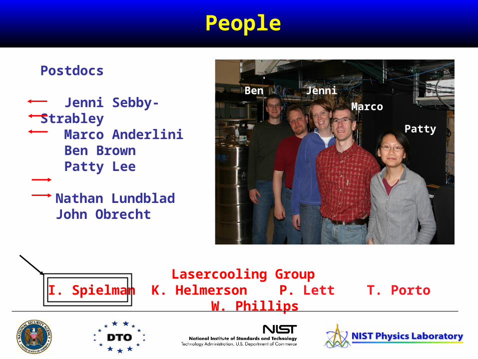
Postdocs

Jenni Sebby-Strabley Marco Anderlini Ben Brown Patty Lee

Nathan LundbladJohn Obrecht

Ben Jenni

Marco

Patty

People

Lasercooling GroupI. Spielman K. Helmerson P. Lett T. Porto

W. Phillips

The End

10-5

10-4

10-3

10-2

10-1

100

4J/E

R

2520151050V/ER

"out of plane" lattice

"in-plane" lattice

Different tunneling

Different J but similar U and vibrational spacing

Same input power

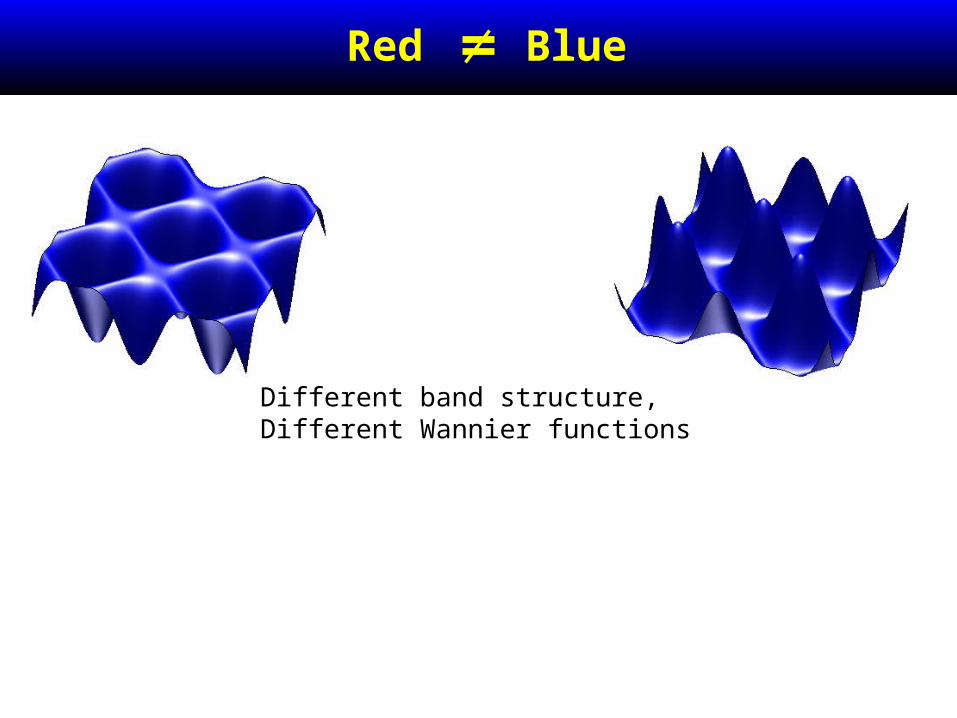
Red Blue

Different band structure,Different Wannier functions

Interesting band structure

e.g. 1/2 filling looks like dimerized hexagonal lattice

2D Mott-insulator

Spielman, Phillips, TP PRL 98, 080404 (2007)

z 2D systems y

x

QuickTime™ and aTIFF (LZW) decompressor


2D Mott-insulator



Quite good comparison to a homogeneous theory (no free parameters)

Sengupta and Dupuis, PRA 71, 033629

Momentum distribution



2D Mott-insulator



Bimodal fit disappears quite sharply

position agrees with theory

(no fit distinction between thermal/depletion)

(non-)adiabatically dressed latttices

RF coupling

-10

-5

0

Potential [ER]

-4-3-2-10

Potential [ER]

8006004002000-200-400Position [nm]

10-6

10-5

10-4

10-3

10-2

10-1

V / U

2 34560.012 3456 0.12 3456 1t/U

5% Tilt15% Tilt3 ER Lattice Depth

Wannier function control

Two band Hubbard modelstate-dependent control of: t/U, /U, position of -lattice

t

Ian Spielman

Characterizing Holes

In a fixed period lattice,difficult to measure “holes”

Isolated holes in /2 Combine holes with neighbors

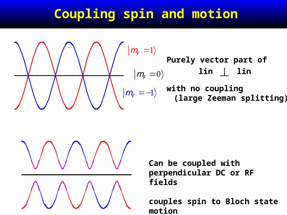
mF =−1

mF =1

mF =0

Can be coupled with perpendicular DC or RF fields

couples spin to Bloch state motion

Purely vector part of

with no coupling (large Zeeman splitting)

lin lin⊥

Coupling spin and motion

Coupling spin and motion

local effective field

alternating plaquettes

Connection between single-particle base states and correlated physics when you put in interactions.

Designing Bose-Hubbard Hamiltonians



State selective motion/splitting

Start with either m=-1 or m=0

Selectively split sites

Tilt dependence of transfer efficiency

or

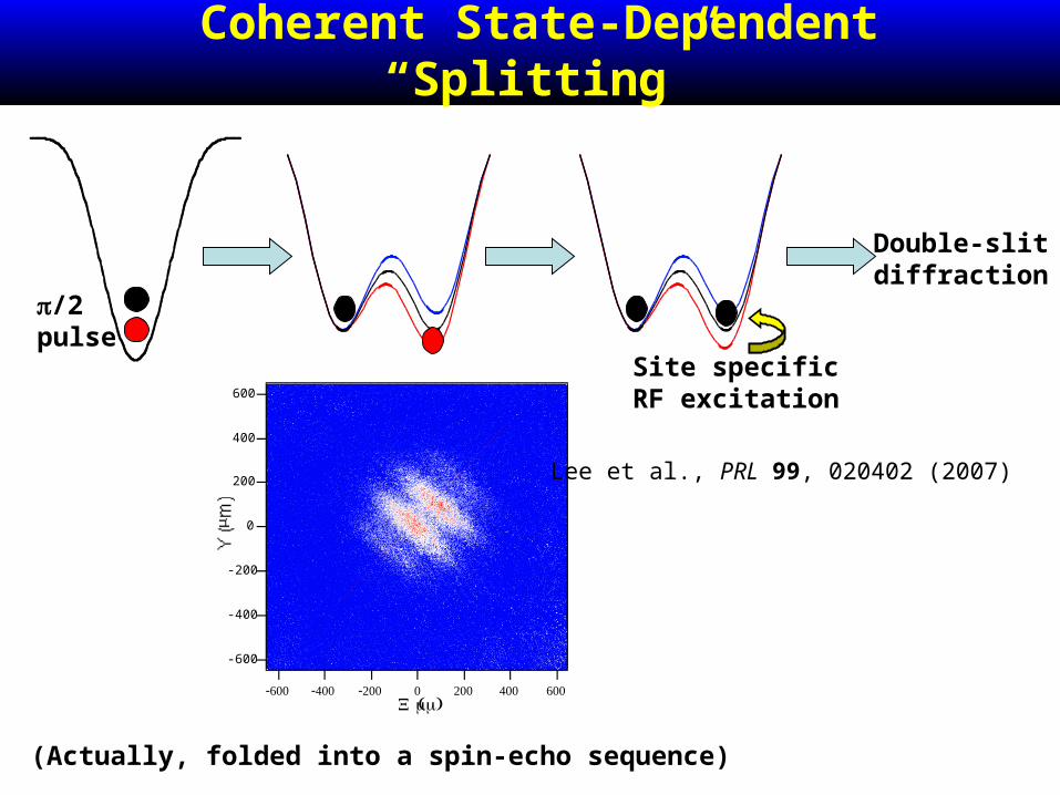
Coherent State-Dependent “Splitting”

-600

-400

-200

0

200

400

600

Y (μ)m

-600 -400 -00 0 00 400 600 (X μ )m

Site specificRF excitation

Double-slitdiffraction

/2 pulse

(Actually, folded into a spin-echo sequence)

Lee et al., PRL 99, 020402 (2007)

Constructing n=2 Shell

n=1 shell,

Normally available n=2 and n=1 shells

n=2 core, n=2 shell,

Adiabatically purify n=2 shell

n=1 shell, /2 n=2 shell,

PRL 98, 200405 (2007)

Documents

1 Trey Porto Joint Quantum Institute NIST / University of Maryland LASSP Seminar Cornell Oct. 30 2007 Controlled exchange interactions between pairs of