1. Unemployment - MIT OpenCourseWare · 1. Unemployment April 9, 2007 Nr. 1 ... Response of Growss Flows Between Employment, Unemployment, and Not in the Labor Force to an Aggregate

1. Unemployment

April 9, 2007

Nr. 1 Cite as: Olivier Blanchard, course materials for 14.462 Advanced Macroeconomics II, Spring 2007. MIT OpenCourseWare (http://ocw.mit.edu/), Massachusetts Institute of Technology. Downloaded on [DD Month YYYY].

2-5. Cyclical movements in unemployment

Implications of the search/bargaining model for cyclical fluctuations?•

Given cyclical fluctuations, job creation, destruction, unemployment?

Explaining cyclical fluctuations. Given shocks, can we explain adjustment? How does it differ from competitive labor market case?

Recessions as times of cleansing/messing up?

Extension of DMP. The “Shimer puzzle”. But linear preferences, and • no nominal rigidities.

Introducing standard preferences. Reinforcing the puzzle. Questioning• Nash bargaining. Wage bands and wage rigidity. Hall.

Introducing nominal rigidities. Blanchard-Gali. How close? How differ• ent from standard NK results?

Nr. 2

Cite as: Olivier Blanchard, course materials for 14.462 Advanced Macroeconomics II, Spring 2007. MIT OpenCourseWare (http://ocw.mit.edu/), Massachusetts Institute of Technology. Downloaded on [DD Month YYYY].

1. Basic facts

Stocks: Beveridge curve movements. Blanchard Diamond Fig 3•

• Job flows: Job creation/job destruction? Foster-Haltiwanger-Kim, 2006, for manufacturing:

Job destruction strongly countercyclical.

Job creation mildly procyclical.

(striking difference by age of plant. Figure 7. (0-3,4-8, 9+)

(Product flows). Paper by Christian Broda. Using USP codes, procycli• cal product creation.

Nr. 3


Image removed due to copyright restrictions.

Figure 8. Beveridge Curve, 1952-88. p. 39.Blanchard, O., and P. Diamond. "The Beveridge curve." Brookings Papers on Economic Activity 1989, no. 1 (1989): 1-60.



Figure 3. Quarterly Job Flows in Manufacturing, 1947-2005. p. 33.Davis, S. J., R. J. Faberman, and J. Haltiwanger. "The Flow Approach to Labor Markets: New Data Sources and Micro-Macro Links." NBER Working Paper No. 12167, April 2006. pp. 1-41. (http://www.nber.org/papers/w12167 )

Nr. 5


From job flows to workers flows: •

Recession: As layoffs increase, quits may decrease.

Layoffs may go from E to U. Quits from E to N, or E to E.

Worker flows. Blanchard Diamond Figure 9. Note asymmetry U, N. In • recession, flow to U increases, flow to N decreases.

Note increase in flow from U to E after 6 months. Strange? No. Difference flow/exit rate

• Exit rates. Blanchard Diamond Fig 13. In recession, more likely tobecome unemployed. Less likely to become employed if unemployed.

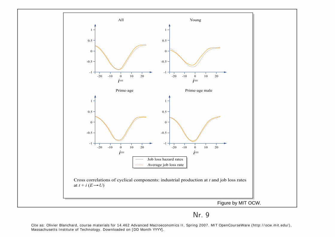
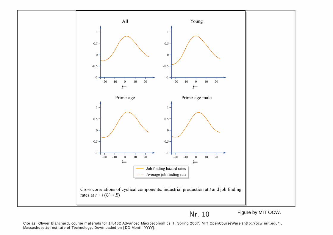
Another way of looking at this. Fujita-Ramey. Cross-correlations between cyclical components of separations/hirings with IP. Figures 13 and 14. Need to put them in.

The revisionist view (Hall) Separations a-cyclical. Not right. (Fujita and • Ramey).

Nr. 6



Figure 9. Response of Growss Flows Between Employment, Unemployment, and Not in the Labor Force to an Aggregate Activity Shock, over Selected Intervals. p. 117��

Blanchard, O., and P. Diamond. "The cyclical behavior of the gross flows of US workers." Brookings Papers on Economic Activity 1990, no. 2 (1990): 85-155.



Figure 13. Response of Hazard Rates Between Employment, Unemployment, and Not in the Labor Force to Aggregate Activity Shock. p. 121.

Blanchard, O., and P. Diamond. "The cyclical behavior of the gross flows of US workers." Brookings Papers on Economic Activity 1990, no. 2 (1990): 85-155.



20100

i=-10-20

-1

-0.5

0

0.5

1

20100

i=-10-20

-1

-0.5

0

0.5

1

20100

i=-10-20

-1

-0.5

0

0.5

1

20100

i=-10-20

-1

-0.5

0

0.5

1

All Young

Prime-age malePrime-age

Cross correlations of cyclical components: industrial production at t and job loss ratesat t + i (E U)

Job loss hazard ratesAverage job loss rate

Figure by MIT OCW.


20100

i=-10-20

-1

-0.5

0

0.5

1

20100

i=-10-20

-1

-0.5

0

0.5

1

20100

i=-10-20

-1

-0.5

0

0.5

1

20100

i=-10-20

-1

-0.5

0

0.5

1

All Young

Prime-age malePrime-age

Cross correlations of cyclical components: industrial production at t and job findingrates at t + i (U E)

Job finding hazard ratesAverage job finding rate

Figure by MIT OCW.

2. Productivity shocks and unemployment in DMP

Based on Shimer (2005)

Standard DMP, exogenous separation, extended to allow for aggregate • shocks.

Two types of aggregate shocks. Shocks to y and shocks to s, but I shall• ignore the shocks to s here.

Go back to the basic equation characterizing equilibrium θ(≡ v/u) (re• call q(θ) ≡ h/v):

(r + s) q(c

θ) = (1 − β)(y − b) − βθc − c

q

q

(

�(θ

θ

)) 2 θ


� =

Here the equation takes the slightly modified form: •

c(r + s) = (1 − β)(y − b) − βθc − cλ(Eq(θ�) − q(θ))

q(θ)

where λ is the Poisson arrival rate of aggregate shocks.

Use this equation to look at θ and by implication, unemployment, in • response to shocks.

First ignore the last term. Define � as the elasticity of θ to y − b. It is• given by:

r + s + βθq(θ) (r + s)(θq�(θ)/q(θ) + βθq(θ)

Nr. 12


� =

If h = m = uαv1−α, then •

r + s + β(h/u) (r + s)(1 − α) + β(h/u)

Now put values, with time unit a month. r ≈ 0.0, s ≈ 0.0 relative to • (h/u) = .4. So � ≈ 1.0.

Take a productivity shock of 1%. If b = .4y, leads to an increase in y − b of (1/.6)%, and so an increase in v/u of (1/.6)%. In the data, σv/u = 38%

So very small movements in u and v.•

Nr. 13


Behind the scene: the adjustment of the wage: •

w = (1 − β)b + β(y + cθ)

To fit the steady state facts (for β = .7) c = .2. So an increase in y of• 1% leads to an increase of .7 (1% + .2 1%) = 0.9%.

Turning to full dynamics. Assume AR(1) process for productivity, with• ρ = .996, and σ = 0.0165. (in continuous time, but irrelevant here)

Table 3 from Shimer. No action.



Table 3. Labor Productivity Shocks. p. 39.

Shimer, R. "The Cyclical Behavior of Equilibrium Unemployment and Vacancies." American Economic Review 95, no. 1 (2005): 25-49.



Figure 5. Response of Unemployment to Negative Impulse, Model and Actual. p. 62.

Hall, R. "Employment Fluctuations with Equilibrium Wage Stickiness." American Economic Review 95, no. 1 (2005): 50-64.


Ways out?

Very small surplus (Hagedorn-Manovskii). y − b. Suppose b = .95.• Then, increase in v/u is 20%. Convincing? No.

• Wage rigidity. Wage can be anywhere in wage band. If aggregate fluctuations not too large, wage can be constant. Hall.

• Constant wage for existing matches: irrelevant. Same wage for new matches as for old matches.

Evidence? Carneiro Portugal. IZA WP 2604. (Useful survey as well) •

Much stronger procyclicality for hires and for stayers (Portuguese data)

Stayers. 1% decrease in u: 1.0% increase in earnings.

New hires: 1% decrease in u: 2.0% increase in earnings.

Relate to computations above? Productivity shocks?•


Need to extend the model further.

Concave preferences •

Nominal rigidities. From wages to inflation. •

Non-tech shocks. •


3. l ntroducing concave preferences

Households

Representative household, continuum of members, [O, I]

where

O < N t < l

Note: Utility specification standard from NK model, but different from DMP model. Bodies, not hours margin. Usual-and unappealing-consumption Insurance.

Nr. 19

Cite as: Olivier Blanchard, course materials for 14.462 Advanced Macroeconomics 11, Spring 2007. MIT OpenCourseWare (http://ocw.mit.edu/), Massachusetts Institute of Technology. Downloaded on [DD Month W].

Firms

Continuum of monopolistically competitive firms, each producing a differentiated good, i ∈ [0, 1] (no capital)

Technology: Yt(i) = At Nt(i)

Employment Nt(i) = (1 − δ) Nt−1(i) + Ht(i)

(δ constant. no endogenous separations)


The labor market

Beginning-of-period unemployment (given full participation): •

Ut = (1 − Nt−1) + δNt−1 = 1 − (1 − δ)Nt−1

Aggregate hiring • Ht = Nt − (1 − δ) Nt−1

Index of labor market tightness (central variable in what follows; deter• minant of marginal cost, of inflation)

Ht xt ≡

Ut ∈ [0, 1]

End-of-period unemployment: •

ut ≡ 1 − Nt


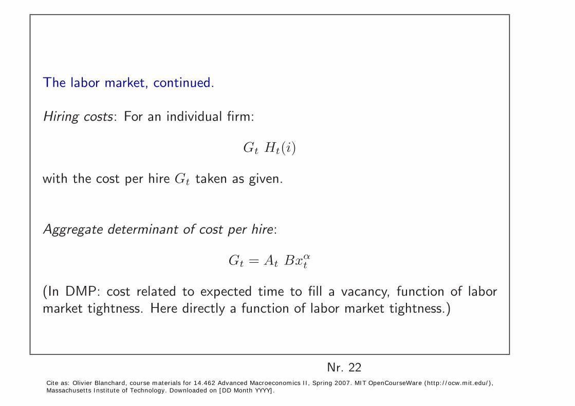
The labor market, continued.

Hiring costs: For an individual firm:

Gt Ht(i)

with the cost per hire Gt taken as given.

Aggregate determinant of cost per hire:

BxαGt = At t

(In DMP: cost related to expected time to fill a vacancy, function of labor market tightness. Here directly a function of labor market tightness.)


(Relation of this assumption to conventional DMP)

In DMP, expected cost of a vacancy proportional to expected duration, V/H. Assume a matching function:

H = zUηV 1−η

Then:η

V H 1−η 1/= z (1−η) ( )

H U So

V = Bxα

H

where B ≡ z1/(1−η) and α = η/(1 − η)

Cost of formalization: No explicit variable for vacancies.

Nr. 23


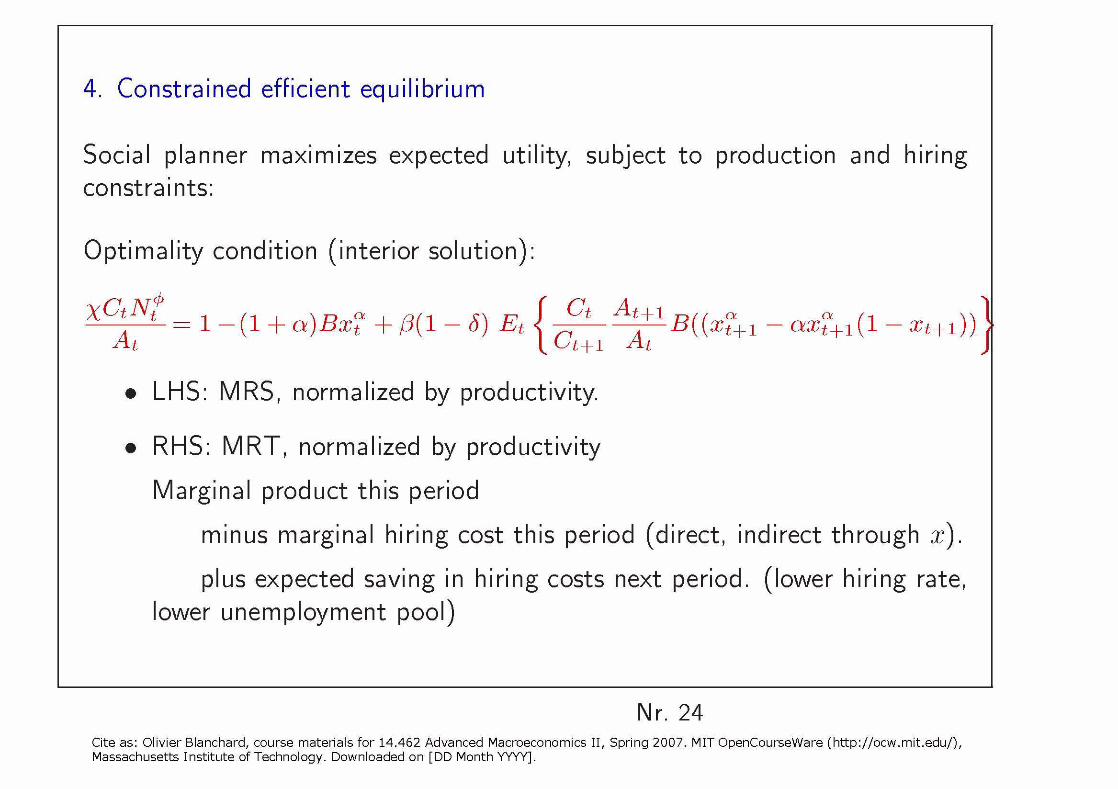
4. Constrained efficient equilibrium

Social planner maximizes expected utility, subject t o production and hiring constraints:

Optimality condition (interior solution):

xct N! ct . = 1 - ( I + a)Bxy + At+l P ( 1 - 6) Et axt"+1(1 - ~ t + l ) )

At { C t + At B((~t"+l - #

LHS: MRS, normalized by productivity.

RHS: MRT, normalized by productivity

Marginal product th is period

minus marginal hiring cost th is period (direct, indirect through x).

plus expected saving in hiring costs next period. (lower hiring rate, lower unemployment pool)

Nr. 24 Cite as: Olivier Blanchard, course materials for 14.462 Advanced Macroeconomics 11, Spring 2007. MIT OpenCourseWare (http://ocw.mit.edu/), Massachusetts Institute of Technology. Downloaded on [DD Month W].

Implications

Looks like a rich dynamic equation. And it is. But: •

With respect to productivity shocks: •

Constant employment, hiring rate.

Consumption moves one for one with productivity.

(Check that Ct/At, Nt, xt = ct is a solution with respect to movementsin At).

Invariance of employment to productivity shocks: Income/substitution• effects, and no capital accumulation.

Model inherits RBC implications (take B = 0), now for unemployment.

If capital accumulation, then some action, but close to RBC.


Compare to DMP, and the Shimer conclusions. •

Ct Ntφ instead of b.

Put another way: Reservation wage adjusts one for one with productivity.Nothing else matters.

A much stronger (and more depressing) result than Shimer.


Useful for later to give a graphical representation of the equilibrium

Dashed blue lines: No frictions. •

Solid red lines: •

MRT/A < 1 : Increasing marginal cost of hiring

MRS/A lower: Lower consumption due to hiring costs.

Nr. 27


(MRS/A)

1 NN*

1

The constrained efficient allocation

MRT/A

Nr. 28


5. Decentralized equilibrium

Price setting by monopolistic competitors:

Optimality condition:

Pt(i) €

= M Pt MCt where M = 6 - 1

where

Symmetric Equilibrium:


Real wages determined by Nash bargaining:

Assume workers get I9 of surplus (used /3 already). Then.

wt - xCtN,'P -- + dBxt" - P(1- 5 ) Et At At { (1 - xt+l) .rP Bxt"+l

At+1 At

Implications:

Constrained efficient? If A4 = 1 and I9 = a: Hosios-like condition.

Efficient or not: Employment (unemployment) invariant t o productivity shocks. (Income/substitution effects, and no capital accumulation)

Real wages move one-for-one with productivity. Wt = O At


Graphical representation of the equilibrium

Solid red lines: Constrained efficient •

Dashed lines: Decentralized equilibrium •

MRT/A: Lower (monopoly power). Flatter: firms do not take into account externalities.

MRS/A higher: Bargaining gives workers some of the surplus.

• Figure 2: Inefficient. Figure 3: Efficient. In both, involuntary unemployment: W > MRS. Participation?

Note: wage band: CD. •


(MRS/A)

1 NN*

1

Equilibrium with Nash bargaining.

1/M

Nnb

A

B

Nr. 32


1 NN*

1

Efficient equilibrium with Nash bargaining.

Nnb =

A

BW/A

(1- B) C

D


6. Rigid real wages

Wi th in the bargaining band-assume tha t real wages follow:

Wt = O A, 1-Y

so y degree o f real wage rigidity (and A is stationary). (Very rough: A better

specification: Wt = (@At) 1-7 W t 7 bu t less tractable)

Implications:

00

= C(P(1 - 6))"t k =O

where At,,+, = (Ct/Ct+k) (At+k/At)

If y > 0, productivity movements affect hiring, and in tu rn lead t o (inefficient) unemployment fluctuations. (relevant equation t o go back t o Shimer calibration.)


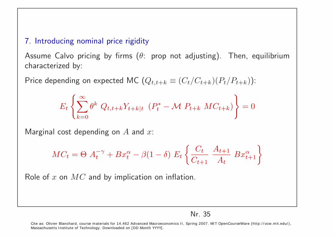
7. Introducing nominal price rigidity

Assume Calvo pricing by firms (θ: prop not adjusting). Then, equilibrium characterized by:

Price depending on expected MC (Qt,t+k ≡ (Ct/Ct+k)(Pt/Pt+k)): � ∞

�

θkEt

� Qt,t+kYt+k|t (Pt

∗ −M Pt+k MCt+k) = 0 k=0

Marginal cost depending on A and x:

MCt = Θ A−γ + Bxα − β(1 − δ) Et

� Ct At+1

Bxα

�

t t t+1Ct+1 At

Role of x on MC and by implication on inflation.


A simple approximation

After log-linearization and dropping second-order terms (hats: deviations from steady state):

∞βkπt = αgMλ xÞt − λΦγ

� Et{at+k}

k=0

uÞt = (1 − δ)(1 − x) Þ − (1 − u)δ xÞtut−1

Interpretation.

Static relation π, x given current and expected productivity? Reflects the samedependence on the expected future.Implication: credibility determines position on trade-off, not position of trade-off.


Back to the inflation-unemployment relation

Assume log productivity follows a stationary AR(1), with parameter ρa. Then:

πt = αgMλ xÞt − Ψγ at

Or

πt = −κ(1 − (1 − δ)(1 − x)) uÞt − κ(1 − δ)(1 − x) Δut − Ψγ at

Note

Level and rate of change of unemployment rate. Relative weights depend • on x. More sclerotic market: more weight on Δu.

If γ > 0, no “divine coincidence” in the presence of productivity shocks.•

Cannot stabilize both unemployment and inflation. (Recall constrained efficient unemployment is constant).


Ad-hoc monetary policies:

Assume a follows an AR(1) with ρ = .9 (quarterly)

Two labor markets; “Fluid”: US: x = .7 (quarterly), u = .05. “Sclerotic”: Europe x = .25 (quarterly), u = 0.10.

Unemployment stabilization (constrained efficient unemployment is con• stant.) Higher inflation in response to negative productivity shock. 0.8% for 1%.

• Inflation stabilization. (Unemployment equal to natural rate, suboptimal). (Very) large increase in unemployment in response to negative shock.

Larger in Europe than in the US: 9% versus 6%: x more closely related to Δn, and thus Δu.

Nr. 38



FJao

Text Box


Optimal monetary policy

Welfare function:

∞βt 2E0

� (πt

2 + αu uÞt ) t=0

Back to optimal monetary policy. Figure 5.

Accept more inflation for some time. •

Large gains in terms of smaller (inefficient) unemployment fluctuations. • (from 9% to 0.5% for Europe, 6% to 1.1% for the US)

Nearly optimal Taylor rules:

For the US: it = 1.5πt − 0.2ut

For Europe it = 1.5πt − 0.6ut


Conclusions/Extensions:

Can the NK+DMP model explain fluctuations?

Model gives us a tool to think about: •

relation between productivity shocks, unemployment, and inflation.

the role of monetary policy in the transmission of shocks.

Practical implications. •

Labor market differences matter for inflation-unemployment relation.

No divine coincidence. Flexible inflation targeting.

Obvious research agenda items. •

Nature, extent, origins of real wage rigidities. Internal organization of firms?

Back to the Shimer puzzle, with inflation/real wages/unemployment, and productivity and non productivity shocks.

Nr. 41


Documents

1. Unemployment - MIT OpenCourseWare · 1. Unemployment April 9, 2007 Nr. 1 ... Response of Growss Flows Between Employment, Unemployment, and Not in the Labor Force to an Aggregate