11. MR Contrast Agents - Universitetet i · PDF file11. MR Contrast Agents ... relaxation times and the distinction between T1- and T2- enhancing agents is therefore somewhat artificial

FYS-KJM 4740 - The Physics of MRI 129

11. MR Contrast Agents In order for an excited spin system to return to its equilibrium magnetization, energy must be transferred from the spin system to the lattice (surrounding), as discussed in Chapter 1. The return to equilibrium is described by the spin-lattice relaxation time, T1. When T1-weighted sequences are used, the magnitude of the MR-signal increases with decreasing T1-relaxation times. Further, the contrast between two tissues will of course also increase with increasing difference in T1 relaxation times between the two tissues. However, the inherent difference in T1 relaxation time between biological tissues, or between normal and pathologic tissue is not always large enough to obtain a detectable contrast in the MR image. Sufficient contrast is of particular importance in differentiating pathological tissue from normal surrounding tissue. Exogenous MR contrast agents were therefore developed shortly after the first commercial MR systems became available in the early 1980’s. Today, MR contrast agents are typically in a significant proportion of MR examinations; with the highest usage in CNS applications (tumor diagnosis). MR contrast agents are also widely used in MR angiography (MRA). MR contrast agents act by selectively reducing T1 (and T2) relaxation times of tissue water through spin- interaction between electron spins of the metal-containing contrast agent and water protons in tissue and in the following sections we shall discuss in some details the mechanism of action of these agents and how it affects the MR signal intensity in vivo.

11.1. Classification of MR contrast agents Although gadolinium based agents are by far are the most commonly used class of MR contrast agents to date, many other types of agents have started to appear on the market. The different classes of contrast agents can be classified according to 1) the magnetic property of the agent, 2) the dominant effect of the agent on the signal intensity and 3) the bio-distribution of the agent. Figure 11-1summarizes the different classes of agents according to these properties.

11.1.1. Magnetic properties Paramagnetism Most MR contrast agents in clinical use to date are based on the paramagnetic metal ions. Paramagnetic materials are metals with unpaired electrons in the outer orbital shells (transition and lanthanide metals), giving rise to magnetic dipoles when exposed to a magnetic field. Since the magnetic moment of an electron is about 700 times larger than that of a proton (due to smaller mass), the paramagnetic ions induce large fluctuating magnetic fields experienced by nearby protons. If the frequency of this fluctuation has a components close to the Larmor frequency it will result in a significant enhancement of proton relaxation. There are many paramagnetic metal ions that could potentially be used as MR contrast agents but the transition metal gadolinium (Gd3+) is by far the most commonly used. This is due to a favorable combination of many (seven) unpaired

FYS-KJM 4740 - The Physics of MRI

electrons combined with a long electron spin relaxation time which makes this metal a very efficient relaxation enhancing agent. The importance of a long electron spin relaxation time for efficient T Superparamagnetism Superparamagnetic agents are insoluble iron oxide crystals with a core diameteare often referred to as nanoparticles, and each nanoparticle contains several thousand paramagnetic Fe ions (Fe2+ and Fecrystal, the net magnetic moment of the nanoparticle is so large that it greatly exceedthat of typical paramagnetic ionscharacterized by a large magnetic moment in the presence of an external magnetic field but no remnant magnetic moment when the field is zeroalso induce strong enhancement of the Tcomposition of the particles), but their dominant effect is on Tlarge magnetic moment of the nanoparticles. Although superparamagnbe specifically discussed in more detail here, the modes of relaxation enhancement

observed with these agents are similar to the ones observed with gadolinium agents, but, as mentioned, with generally stronger effects on transverse rel

11.1.2. The biodistribution of a contrast agent describes how the agent is distributed in vivo after intravenous administration (all current agents are administered by i.v injection).

Figure 11-1. Classification of MR contrast and dominant image enhamcenement

The Physics of MRI

electrons combined with a long electron spin relaxation time which makes this metal a very efficient relaxation enhancing agent. The importance of a long electron spin

efficient T1-relaxation will be discussed below.

Superparamagnetic agents are based on magnetite (Fe3O4) or maghemite (γ-insoluble iron oxide crystals with a core diameter in the range 5 – 10 nm. These crystals

n referred to as nanoparticles, and each nanoparticle contains several thousand and Fe3+). If the Fe ions are magnetically ordered within the

crystal, the net magnetic moment of the nanoparticle is so large that it greatly exceedtypical paramagnetic ions. This effect is referred to as superparamagnetism and is

characterized by a large magnetic moment in the presence of an external magnetic field but no remnant magnetic moment when the field is zero. Superparamagnetic agealso induce strong enhancement of the T1- relaxation rate of water (depending on size and composition of the particles), but their dominant effect is on T2/T2* relaxation due to the large magnetic moment of the nanoparticles. Although superparamagnetic agents will not be specifically discussed in more detail here, the modes of relaxation enhancement

observed with these agents are similar to the ones observed with gadolinium agents, but, as mentioned, with generally stronger effects on transverse relaxation.

Biodistribution The biodistribution of a contrast agent describes how the agent is distributed in vivo after intravenous administration (all current agents are administered by i.v injection).

Classification of MR contrast agents based on magnetic properties, biodistribution and dominant image enhamcenement

130

electrons combined with a long electron spin relaxation time which makes this metal a very efficient relaxation enhancing agent. The importance of a long electron spin

-Fe2O3) water . These crystals

n referred to as nanoparticles, and each nanoparticle contains several thousand ). If the Fe ions are magnetically ordered within the

crystal, the net magnetic moment of the nanoparticle is so large that it greatly exceeds . This effect is referred to as superparamagnetism and is

characterized by a large magnetic moment in the presence of an external magnetic field . Superparamagnetic agents can

relaxation rate of water (depending on size and * relaxation due to the

etic agents will not be specifically discussed in more detail here, the modes of relaxation enhancement

observed with these agents are similar to the ones observed with gadolinium agents, but,

The biodistribution of a contrast agent describes how the agent is distributed in vivo after intravenous administration (all current agents are administered by i.v injection).

agents based on magnetic properties, biodistribution


ECF agents Small molecular weight (MW) paramagnetic agents are small enough to diffuse from the plasma into the interstitium and are thus distributed to the extracellular fluid. These agents are therefore often referred to as ECF agents. They are not taken up by cells and are therefore eliminated by renal excretion with a half-life determined by the glomerular filtration rate. Intravascular agents Intravascular agents are contrast agents with a MW large enough to prevent leakage from the vascular to the intravascular space. All iron oxide particles are intravascular agents, with a half-life in blood ranging from a few minutes to several hours. Iron oxides are eventually eliminated from the blood by phagocytosies and are thus taken up by the Kupffer cells of the liver, spleen and lymphatic system. In blood, iron oxide agents with the appropriate composition can produce significant T1-shortening – and several studies have investigated the use of nanoparticles for MR angiography. Once taken up by the liver the nanoparticles will be accumulated into larger particulate clusters in the Kupffer cells and relaxation will be completely dominated by T2/T2* effects. Iron oxides can thus be said to be both intravascular agents as well as tissue specific agents. Other types of intravascular agents exist which are based on macromolecular gadolinium compounds. Such agents are designed either by linking Gd3+ ions to a macromolecular polymer during synthesis or by making the Gd3+complex bind to plasma proteins after injection and thus forming macromolecules in blood Tissue specific agents Tissue specific agents are agents which have been specifically designed to accumulate in a given organ or tissue type. We have already seen that iron oxide nanoparticles are liver specific agents (as well as spleen and lymph node specific), and this class of agents have been shown to offer clinical utility in detecting liver lesions (by making normal liver parenchyma dark, rendering liver lesions hyperintense) after contrast agent accumulation in the liver. Other liver specific agents have also been developed, based either on Gd3+ or on the paramagnetic ion Mn2+. Contrast agents have also been developed, and are in clinical testing, for targeting of atherosclerotic plaques as well as different types of tumor antibodies.

11.1.3. Image enhancement The effect of the contrast agent on the signal intensity can either be positive (increase in signal or T1-enhancement) or negative (signal reduction or T2-enhancement). As will be discussed in the next sections almost all MR contrast agents will affect both T1- and T2- relaxation times and the distinction between T1- and T2- enhancing agents is therefore somewhat artificial and will depend on many MR-specific parameters as well as contrast agent dose. In order to quantify the effect of the agent on signal intensity we need to quantify the relaxation enhancing capability of the particular agent in question. This issue will be dealt with the following sections


11.2. Contrast agent relaxivity The ability of a contrast agent to enhance the proton relaxation rate is defined in terms of its relaxivity:

Eq. 11-1

��,� � 1��,� � ��,� �,��

where R0

1,2 are the relaxation rates (R1,R2) without the presence of the contrast agent, C is the (molar) concentration of the contrast agent and r1,2 are the relaxivity constants (T1- and T2-relaxivity) of the agent. The unit of r1 and r2 are mM-1s-1 (where mM = 10-3

mole/Litre). Note that Eq. 11-1assumes a linear relationship between contrast agent concentration and increase in relaxation rate. As will be shown later in the chapter, this is not always the case in tissues in vivo. Paramagnetic relaxation enhancement is commonly divided into inner-sphere and outer-sphere effects. Inner-sphere effects induce both T1- and T2- relaxation and require a direct interaction (binding) between the paramagnetic centre and the water protons (at the hydration site of the paramagnetic ion). The proton T1- and T2-relaxivities due to inner sphere relaxation can be expressed as:

Eq. 11-2

� � � ��

� � �� ∆ω�� ∆ω��

where A is a constant, q is the number of coordinated water molecules per metal ion and τm is the residence time (chemical exchange) of the water molecules at the coordination site of the metal, T1m and T2m are the relaxation times of bound water and ∆ωm is the chemical shift difference between bound water and bulk water. T1m and T2m are complex functions of the properties of the contrast agent and depend strongly on the ability of the water protons to get in close proximity of the paramagnetic centre as well as on the rotational dynamics of the contrast agent molecule. The paramagnetic relaxation theory was originally derived by Solomon and Bloemenberg in the 1950’s and its details are way beyond the scope of this compendium. However, it should be mentioned that the contrast agent relaxivity is strongly dependent on the ‘effective’ correlation time which is given by:

Eq. 11-3 1/�� 1/�� 1/�� 1/��

FYS-KJM 4740 - The Physics of MRI

where τr, τs and τm are the correlation times, respectively, of rotation (of the contrast agent molecule), electron spin relaxation (of the unpaired electrons) and chemicexchange (inverse of the lifetime of binding time of the water molecule to the paramagnetic ion). Proton relaxation due to paramagnetic interaction is related to the correlation times through spectral power density functions of the forms:

and ωS are the proton and electron Larmor frequencies, respectively. It therefore follows that effective relaxation requires that resonance frequencies, respectively. For a given correlation time the relaxivity of paramagnetic agents is thus dependent on field strength with decreasing relaxivity with increasing fields and in the high field limit rwhich is proportional to τc (derivation not shown here)molecular weight of the contrast agent, with larger molecules in general giving slower rotational correlation times. The electron spin relaxation time, of the paramagnetic ion, and for ‘long’ enough to avoid that the overall correlation time 1/ τc too short for effective relaxation to take place). Other paramadysprosium (Dy3+) exhibit very low Tto a very short electron spin relaxation time (10 In addition to the importance of optimal correlation time

agent relaxivity is directly proportional to the number of water molecules (q) directly coordinated to the paramagnetic ion. In the Gdwater molecules, resulting in a high relaxivity. and needs to be incorporated in a ligand to prevent the Gdendogenously available anions.

Figure 11-2. Example of a gadolinium gadolinium ion the a biocompatible

The Physics of MRI

are the correlation times, respectively, of rotation (of the contrast agent molecule), electron spin relaxation (of the unpaired electrons) and chemicexchange (inverse of the lifetime of binding time of the water molecule to the

Proton relaxation due to paramagnetic interaction is related to the correlation times through spectral power density functions of the forms: and

are the proton and electron Larmor frequencies, respectively. It therefore follows that effective relaxation requires that τc and τs are close to the proton and electron

nce frequencies, respectively. For a given correlation time the relaxivity of paramagnetic agents is thus dependent on field strength with decreasing relaxivity with increasing fields and in the high field limit r1 tend to zero whereas r2 approaches a valu

(derivation not shown here). τr is related to the size and molecular weight of the contrast agent, with larger molecules in general giving slower

The electron spin relaxation time, τs, is an intrinsic property of the paramagnetic ion, and for gadolinium is of the order of 10-8 seconds which is ‘long’ enough to avoid that the overall correlation time 1/ τc is dominated by τ

too short for effective relaxation to take place). Other paramagnetic ions, like ) exhibit very low T1-relaxivity in spite of seven unpaired electrons due

to a very short electron spin relaxation time (10-13 sec).

In addition to the importance of optimal correlation time τc, we observe that the contr

agent relaxivity is directly proportional to the number of water molecules (q) directly coordinated to the paramagnetic ion. In the Gd3+ aqua ion there are eight innerwater molecules, resulting in a high relaxivity. However, the Gd3+ ion itself is rather toxic and needs to be incorporated in a ligand to prevent the Gd3+ ion to interact with endogenously available anions. The ligand is a biocompatible molecule which binds

Example of a gadolinium chelate (GdDTPA-BMA) formed by covalent binding of the patible ligand

133

are the correlation times, respectively, of rotation (of the contrast agent molecule), electron spin relaxation (of the unpaired electrons) and chemical exchange (inverse of the lifetime of binding time of the water molecule to the

Proton relaxation due to paramagnetic interaction is related to the correlation times where ωI

are the proton and electron Larmor frequencies, respectively. It therefore follows are close to the proton and electron

nce frequencies, respectively. For a given correlation time the relaxivity of paramagnetic agents is thus dependent on field strength with decreasing relaxivity with

approaches a value is related to the size and

molecular weight of the contrast agent, with larger molecules in general giving slower insic property

seconds which is is dominated by τs (making

gnetic ions, like relaxivity in spite of seven unpaired electrons due

e observe that the contrast

agent relaxivity is directly proportional to the number of water molecules (q) directly aqua ion there are eight inner-sphere

is rather toxic ion to interact with

The ligand is a biocompatible molecule which binds

BMA) formed by covalent binding of the


strongly to the paramagnetic ion to form a stable metal chelate. Many different gadolinium chelates are available for clinical use today; most of which are small molecular weight agents with a molecular weight (MW) of the complete chelate of less than 1000 daltons. Figure 11-2 shows the configuration of one commercially available gadolinium chelate (GdDTPA-BMA, OmniscanR). We see that a the gadolinium ion is surrounded – and tightly bound- to a ligand which occupy seven of the eight available bindings sites of the gadolinium – leaving a single binding site available for water. The effective T1-relaxivity (r1) of this (and many similar) gadolinium chelate is about 4 mM-1s-1 (at 20 MHz) and the T2-relaxivity is slightly higher. It should be stressed that the relaxivity of MR contrast agents is usually measured in water (at specified field strength and temperature) and the effective in vivo relaxivities may differ significantly from the in vitro values, as discussed in later sections.

11.3. In vivo relaxivity and MR contrast enhancement We have seen in the previous section that the efficiency of a contrast agent to enhance the relaxation rates 1/T1 and 1/T2 is defined in terms of the relaxivities (r1,r2) of the agent. We shall now discuss in more detail the effect of relaxation enhancing agents on the MR signal intensity. In addition to the ‘dipolar’ relaxation effects discussed above, there is an additional contrast agent relaxation effect due to local variations in the Larmor frequency induced by the magnetic moment of the contrast agent. This is commonly referred to as ‘susceptibility induced relaxation’ and will be discussed in more details below. But first we will discuss the effects of dipolar relaxation resulting from a direct interaction between water protons and the paramagnetic centre.

11.3.1. Dipolar relaxation It should initially be mentioned that, unlike e.g. in CT, the ‘dose response’ due to MR contrast agents in general highly non-linear. This means that the effect of the agent (on the measured MR signal intensity in a given sequence) is not linearly related to the contrast agent concentration in a given voxel. This may not be a major problem if we are only interested in a qualitative assessment of contrast agent enhancement, but it is a major problem if we need to relate the change in signal intensity to absolute (or even relative) concentration. From the expressions for contrast agent induced change in relaxation rates, given in Eq. 11-1 the corresponding changes is MR signal intensity can readily be estimated for a given pulse sequence given that the relaxivity values (r1,r2) of the agent are known. Assuming a SE sequence, the SI change due to the contrast agent is thus given by:

Eq. 11-4 �� 1 exp � �� exp � �� $


where r1, r2 are the T1- and T2- relaxivities, respectively, for the agent, C is the contrast agent concentration and R0

1, R02 are the T1- and T2- relaxation rates, respectively, without

the contrast agent. Figure 11-3 shows the change in SI as a function of CA concentration, assuming ρ=100, r1=4 mM-1s-1 and r2=4.5 mM-1s-1, R0

1=1 s-1 and R02=4 s-1, TR=500 ms

and TE=30 ms. As seen, the dose response is highly non-linear. However, within an initial concentration range, a fairly linear increase in SI is observed with increasing concentration. At higher concentrations, signal saturation occurs meaning that a further reduction in T1

does not result in a further increase in SI since the longitudinal magnetization is fully recovered. Further, when the concentration becomes very high (depending on the TE) the signal will start to fall with further increase in C since the T2-effects of the contrast agent will start to dominate the signal behavior. Figure 11-4 shows a sample of a patient with a brain tumor imaged with a SE sequence before (left) and after administration of a gadolinium based ECF-agent. Note the strong local T1-enhancement in the rim of the tumor. The contrast agent does not leak out from the intravascular space in normal brain tissue due to the presence of a blood-brain-barrier (BBB) which prevents even small MW molecules like Gd-chelates to enter the intenstitium. Since the intravascular volume in the brain is small (< 5%) little enhancement is thus seen in healthy brain tissue. In brain tumors, however, the BBB can often be disrupted due to various pathological processes, resulting in a selective accumulation in the extravascular space in the tumor, as seen in the figure. The fact that many pathological processes alter the permeability of the BBB, resulting in selective accumulation of the MR contrast agents is, in fact, the main reason why these agents are so useful for CNS imaging since the absence/presence of CA leakage as well as the pattern of contrast enhancement can give important indications as to the type of pathology present. Therefore MR contrast agents not only increase the

0 1 2 3 4 530

40

50

60

70

80

CA concentration (mM)

Rel

SI

Figure 11-3. Simulated dose response of an MR contrast agent (CA) in a SE sequence. Initially T1-relaxation dominated but as the CA concentration becomes sufficiently high T1-saturation as well as counter-acting T2-relaxation becomes dominant resulting in signal reduction at higher concentrations


sensitivity (the ability to detect) but also the specificity (the ability to differentiate) of the diagnostic procedure.

We observed in the simulation of Figure 11-3 that at high CA concentrations, the SI fell with further increase in CA concentration, even in a highly T1-weighted SE sequence. This can of course be a problem if, for some reason, the local CA concentration is so high that the signal has returned to baseline due to counter-acting T2-effects, thus giving the false impression of no contrast agent being present. In other situations, the T2-relaxivity of MR contrast agent is utilized specifically for different diagnostic purposes. This leads us on the topic of susceptibility induced relaxivity and will see that the T2-relaxivity of MR contrast agents in vivo in many situations, in fact is much higher than what is predicted by just the dipolar component discussed so far.

11.3.2. Water exchange effects Dipolar relaxivity is dependent on direct interaction between water protons and the paramagnetic centre of the contrast agent. The linear relationship between relaxation rate and contrast agent concentration assumes that all protons which contribute to the MR signal have equal and unrestricted access to the paramagnetic ion on a time-scale equal to the T1 relaxation time of the medium. This condition is referred to as ‘fast exchange’ and the requirement for fast exchange can be expressed in terms of a correlation time, τ, so that:

Eq. 11-5 1� % 1/��,� 1/��,�

where 1/ τ is the rate of water exchange between the compartments with relaxation rates 1/T1,1 and 1/T1,2, respectively. In vivo, the two compartments can for instance be the

Figure 11-4. Example of the effect of a Gd3+-based ECF agent in a patient with a brain tumor. The contrast agent is selectively taken up in the tumor region due to pathological changes in the blood brain barrier (BBB) whereas an intact BBB prevents contrast agent accumulation in unaffected brain tissue.


intravascular and the extravascular (interstitial) compartment or the intra- and extracellular compartments of the extravascular space. The effect of limited water exchange on proton relaxation can be addressed by addition of a two-site water exchange terms to the Bloch equation describing the rate of magnetization between two compartments:

Eq. 11-6 &'�&( � '� '��,� )�'� )�'�

&'�&( � '� '��,� )�'� )�'�

where 1/T1,1, 1/T1,2 are the longitudinal relaxation rates of the two compartments, M0 is the equilibrium magnetization for the two compartments and k1, k2 are the water exchange rates between the two compartments. Figure 11-5 shows a schematics illustration of the water exchange process between the intravascular compartment (containing gadolinium) and the extracellular compartment. The exchange rate 1/τ introduced in Eq. 11-5 is the sum of the two rate constants k1+k2 so that 1/k1 (τ1) and 1/k2 (τ2) describe the average lifetime of the spins within the two compartments. The rate constants k1 and k2 are related (through mass balance) and k2 can be expressed in terms of k1 as follows:

Eq. 11-7

)� � )� *�+ *�

where ξ1 is the relative volume of compartment 1 and λ is the ratio of proton spin densities in compartment 2 vs compartment 1. The general solution to Eq. 11-6 is described by a bi-exponential function of the form:

Eq. 11-8 '�(� � '� ,� exp� -�(� ,�exp � -�(� where c1,c2,u1,u2 are functions of k1,k2, 1/T1,1 and 1/T1,2. It can be shown that if the volume of compartment 1 is small or fast exchange conditions apply then Eq. 11-8 is well approximated by the well known mono-exponential relaxation curve following an inversion (180o) RF-pulse:

Eq. 11-9 '�(� � '��1 2 exp� ��(��


Figure 11-5. Schematic illustration of water exchange between two tissue compartments; one containing contrast agent (intravascular space) and an extravascuclar space.

where R1 is now the ‘effective’ tissue relaxation rate of a two-compartment system and is given by:

Eq. 11-10

�� / -� � 12 ��,� )� ��,� )�� 12 0��,� )� ��,� )�� 4)�)�

The effective tissue relaxation rate in a two-compartment system is thus a highly non-linear function of the relaxation rates in the two tissue compartments and the rate of water

Figure 11-6. Simulations of the relationship between R1 in blood and measured effective R1 in tissue in a two-compartment system with different water exchange rates between the two compartments.


exchange between them. Figure 11-6 shows sample curves of R1 in tissue (i.e. in an image voxel containing both compartments) vs R1 in blood for different exchange rates k1. The initial slope of the R1-curve describes the fast exchange limit (R1,1-R1,2 << k1) and scales with the blood volume of the intravascular compartment. In the opposite extreme of slow exchange limit (R1,1-R1,2 >> k1) the value of R1 becomes independent of R1 in blood and approaches asymptotically a maximum value given by: R1

max=R1,2+k2.

Exchange limitations are of particular importance in the brain because the contrast agent is usually confined to the intravascular compartment due to the blood brain barrier. The water exchange rate across the capillary membrane is of the order of 100 ms, and the achievable T1-enhancement in the brain (with no BBB leakage) is thus limited by the intravascular blood volume and the water exchange constant. The non-linear dose-response in terms of 1/T1 is again of particular importance when the contrast agent concentration needs to be estimated based on the MR signal response, as for instance is the case in MR perfusion imaging. Figure 11-7 summarizes the expected R1 dose response in different tissues as a function of tissue blood volume and exchange rates. Note that a linear response is expected in blood due to fast water exchange (<10 ms) between plasma and the intracellular compartment of the erythrocytes.

Figure 11-7. Summary of expected R1 dose-response in vivo in a two compartment system (typically brain

tissue) after contrast agent enhancement.

11.3.3. Susceptibility induced relaxation. Magnetic susceptibility effects were discussed in Chapter 1069.1and we defined susceptibility as the proportionality constant between applied magnetic field and induced tissue magnetization: Mz=χH0 (H=Bo/µ0). We also mentioned in Chapter 1069 that a


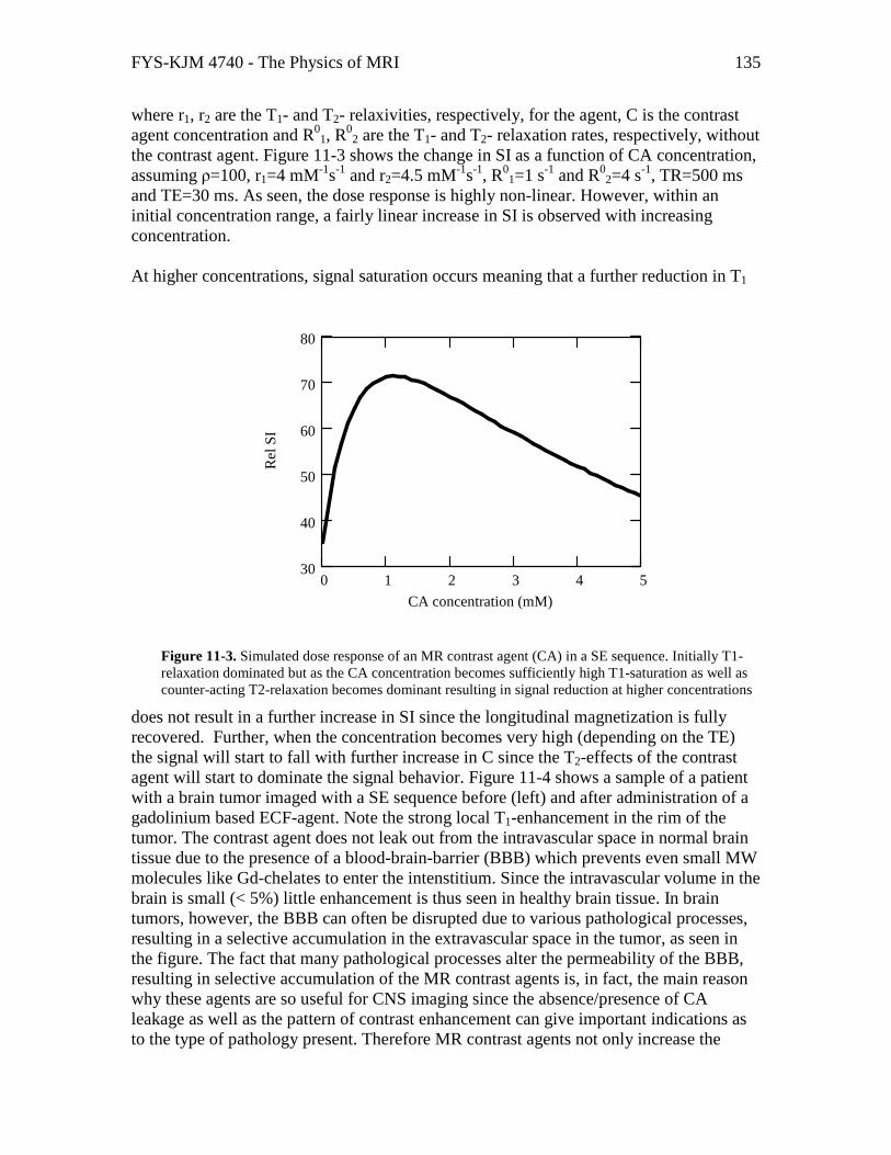
similar relationship existed for paramagnetic agents. The general theory describing the relationship between induced magnetization M and applied magnetic field H0, valid at all fields, is expressed classically by the Langevin function:

Eq. 11-11

' � 23 4,5(6 78�39�):� ; 7 ):�8�39�;< where N is the number of paramagnetic atoms per unit volume, m is the magnetic moment per atom, kB is the Boltzmann’s constant and T is temperature in Kelvin. For values of µ0mH0/kBT <<1 (valid for field strengths below approx 50 T!) this leads to the approximation:

Eq. 11-12

' � 23�8�9�3):� � >9�

With

Eq. 11-13

> � 23�8�3):�

where Eq. 11-13 is known as the Curie law (compare to Eq. 1-3 for nuclear susceptibility). It can therefore be concluded that, for paramagnetic contrast agents, the induced magnetization is proportional to the applied magnetic field and the concentration of contrast agent in tissue (N) and the square of the magnetic moment of the paramagnetic ion. As discussed in Chapter 9, transverse relaxation will therefore be enhanced if the contrast agent is unevenly distributed in tissue so that local susceptibility differences occur. This is referred to as susceptibility induced relaxation and only affects T2/T2* and not T1-relaxation. In fact, a contrast agent is almost always unevenly distributed in vivo due to multiple intra- and extracellular compartments. Most existing MR contrast agents are ECF agents and thus distribute to the extracellular compartments (blood plasma and interstitium). This means that local susceptibility differences due to the contrast agent will occur both in blood and in the interstitium, giving rise to enhanced T2 and T2* relaxation. The susceptibility effect does not affect the longitudinal relaxation times in tissue because the size of the field perturbing compartments in vivo are so large that the T1-relaxivity has dispersed to zero at clinical fields. This is an important point because it reflects a fundamental property of the proton relaxation enhancing processes induced by contrast agents; a contrast agent can induce T2/T2* relaxation without affecting T1 if the combination of field strength, the magnetization due to the perturber (the magnetic agent) and the size of the perturbation is such that T1-relaxivity has dispersed to zero. Any reduction in T1 does, however, always cause a reduction in T2/T2* since T2-relaxation is caused by the same relaxation mechanisms which causes T1-


relaxation – but includes an additional term which is independent of field fluctuations so that T2/T2* relaxation does not disperse to zero at any fields. Given that the contrast agent is unevenly distributed in tissue, the resulting variation in susceptibility ∆χ thus gives rise to a local variation in Larmor frequency ∆ω=γ∆χB0, with consequent loss of MR signal due to transverse relaxation. The resulting T2/T2* ‘relaxivity’ due to susceptibility effects is a complex function of many parameters; including sequence type (SE vs GRE), tissue structure, contrast agent properties and dose. One simplification is to assume that protons are ‘static’ in the TE-period; i.e. that the variation in frequency across the voxel due to ∆χ is much larger than the variation in frequency experienced by each proton due to proton diffusion. This is the so-called ‘static dephasing scheme’ and the resulting modulation of MR signal intensity due to ∆ω can then be expressed as:

Eq. 11-14

��$, ?� � �� @ A�?�exp � B?�$�&?∞

�∞

Note that in a static dephasing regime, no additional signal loss will occur in a SE sequence since the effect will be completely compensated for by the 180o pulse. In order to determine the corresponding T2* relaxivity (assuming GRE sequences) due to ∆χ, the frequency distribution within each voxel P(ω) must be known P(ω) can be determined e.g. by spectroscopic (Fourier) analysis of the free induction decay (FID) signal. The proton spectrum is then identified in terms of the linewidth and lineshape of the frequency response. The most commonly observed frequency distribution in vivo is a Lorentzian distribution of the form:

Eq. 11-15

A�?� C D EE� ?�F where σ2 is the variance of the frequency distribution so that the linewidth (in terms of FWHH) of the distribution is given by 2σ. Inserting the expression for P(ω) into Eq. 11-14 we then have:

Eq. 11-16

��$, ?� � �� @ D EE� ?�F exp � B?�$�&? � ��exp � ∞

�∞ E�$�

The effective T2-relaxation due to a Lorentzian field distribution is thus given by T2*=1/ σ and the increase in relaxation rate R2*=1/T2* is proportional to the linewidth of the frequency distribution. If we assume that σ is proportional to the increase in susceptibility due to the contrast agent (a plausible assumption) which again is proportional to the contrast agent concentration (number of paramagnetic molecules per unit tissue), then the


change is signal intensity due to the agent in a T2/T2* weighted sequence (where T1-effects are assumed to be negligible) is given by:

Eq. 11-17 �� 0� exp� E��$� � ��0�exp � )� · �$� where C is the contrast agent concentration and k is a constant. The assumption of a Lorentzian lineshape in vivo may not hold in all tissues, and particularly in blood many studies have shown than the linehape is better approximated by a Gaussian function of the form:

Eq. 11-18

A�?� C IJK L ?�2E� M

The corresponding signal equation thus becomes:

Eq. 11-19

��$, ?� � �� @ IJK L ?�2E� M exp � B?�$�&? � ��exp N �E�$��O∞

�∞

We now see that the ‘effective’ relaxation rate is given by R2=σ

2TE (so that � ��exp � ��$). The effective R2 is thus proportional to TE and to the square of contrast agent concentration, C (assuming again that E C �). Figure 11-9 shows sample spectra for a Gaussian (left) and Lorentzian lineshapes, both measured in blood. The Lorentzian lineshape is observed in fully oxygenated blood (no paramagnetic species) whereas the Gaussian lineshape is observed in deoxygenated blood due to the presence of paramagnetic deoxyhemoglobin or in oxygenated blood containing a paramagnetic contrast agent. Figure 11-8 summarizes the expected R2* dose response as a function of contrast agent concentration (relative units) in different tissues. Note the linear response in tissue (where the slope scales with tissue blood volume) due to a predominant Lorentzian lineshape whereas a quadratic relationship is expected in blood containing contrast agent where the field distribution is better described by a Gaussian function (Eq. 11-18).


Figure 11-9. Example of a Gaussian (left) and Lorentzian lineshape obtained from respective samples of deoxygenated (left) and oxygenated blood.

Figure 11-8. Summary of expected R2* dose response in vivo as function of contrast agent concentration (arbitrary units). A linear response in expected in tissue whereas a non-linear (quadratic) response is expected in blood.


11.4. Further reading Chapter 11

1. Merbach and Tóth (eds). The Chemistry of Contrast Agents in Medical Magnetic Resonance Imaging. John Wiley & Sons, Ltd. ISBN 0-471-60778-9. (2000).

2. Rocklage, Watson and Carvlin. Chapter 14 In Stark and Bradley (eds); Magnetic Resonance Imaging (2nd edition). Mosey Year Book (1992).

3. Bjørnerud. Proton Relaxation Properties of a particulate Iron Oxide MR Contrast Agent in Different Tissue Systems. PhD thesis. Uppsala 2002 (ISBN 91-554-5330-9).


12. Advanced Applications of MR Contrast Agents As we have already seen in the previous chapter, MR contrast agents can be used to modify the MR signal intensity in many different ways, depending on tissue structure, contrast agent type and concentration as well as MR sequence parameters. The ‘classical’ application of MR contrast agents is based on static images where areas of increased contrast agent update secondary to pathology are detected. Such applications still account for the large majority of contrast enhanced MRI. However, there is an increasing use of dynamic analysis of contrast enhancement whereby tissue function can be more directly assessed. Since this is an important area (especially for MR physicist) some of these methods will be discussed in a separate chapter (this one). As we shall see later in the chapter, most dynamic imaging techniques require some sort of estimation of the contrast agent (CA) concentration (or at least relative concentration). We will therefore start by addressing how the CA concentration is related to the measured MR signal using different imaging techniques.

12.1. T1-based dynamic imaging In T1-based perfusion imaging, the sequence is made optimally T1-sensitive and minimally T2/T2* sensitive. The most linear results are obtained if T1-relaxation times are measured directly (e.g. using a saturation recovery or inversion recovery sequence). The great advantage of measuring T1 is thus that transverse relaxation effects as well as signal saturation are completely eliminated. The change in T1 relaxation rate due to the contrast agent is then given by:

Eq. 12-1 Δ��(� � ��(� �� Q�(�� where �� is the T1 relaxation rate before contrast arrival and r1 is the T1-relaxivity of the contrast agent (see Eq. 11-1). Even if r1 is not known the concentration is still known to within a constant as long as we can assume the relaxivity of the agent to be the same in all tissues of interest and that fast water exchange can be assumed between all sub-compartments within each image voxel. The main disadvantage is that it takes time to measure T1-relaxation times and temporal resolution therefore needs to be scarified. An alternative to estimating T1 at each time-point is to acquire images with an extremely T1-weighted GRE sequence. As long as TR<< T1 and TE<<T2* and the flip angle is large the

signal response can then be approximated to �� C RSTUTV (see spoiled GRE equation in

Chapter 4.2). We thus have an approximately linear dose response as long as 1/T1 is proportional to contrast agent concentration (e.g. fast exchange condition described in Chapter 11).


12.2. T2/T2* based dynamic imaging T2- or T2* weighted dynamic imaging is also often referred to as dynamic susceptibility contrast (DSC) imaging. DSC imaging is particularly useful in the brain. Because small MW Gd-agents are effectively intravascular agents in the brain (due to the BBB) the volume of distribution is limited by the cerebral blood volume (less than 5% in the brain). T1-enahncement, being limited by intra- extravascular water exchange is therefore limited in the brain. The susceptibility effect, on the other hand, is a long range effect and will affect protons far outside the intravascular compartment – thereby giving a much larger dynamic signal change compared to the T1-effect. Most DSC sequences are EPI based (either SE-EPI or GRE-EPI). In both cases we can express the dynamic signal response as:

Eq. 12-2 ��(� � ��0�W�'�, ��exp � �$ · Δ��(�� where SI(0) is the signal intensity at baseline (prior to contrast arrival f(T1) is some function of M0 and T1, TE is the echo time and ∆R2 (t) is the change in transverse relaxation rate (1/T2 for SE- or 1/T2* for GRE- based EPI) due to the contrast agent. If we assume T1-effects to be negligible, we then have

Eq. 12-3

Δ��(� � ) ln L��(��0�M /�$ C ��(�

Where C(t) is the dynamic contrast agent concentration. We here assume a mono-

time

Raw data

∆R2* maps

t=0

Figure 12-1. Dynamic T2* weighted imaging following a bolus injection of a gadolinium based ECF agent. The top row shows the raw data and the bottom row the R2*-converted images using Eq. 12-3. The contrast agent was injected at t=0. Note the negative (T2*) effect of the contrast agent in the raw images whereas the effect is positive and scales with CA concentration in the R2* images.


exponential relationship between Δ�� and SI and a linear relationship between Δ�� and C (in other words a Lorentzian lineshape as discussed in previous chapter). Figure 12-1 shows an example of DCS images before and after conversion to Δ��. The dynamic series of Δ�� maps are used for further analysis of different perfusion related parameters as will be discussed in the next section.

12.3. Perfusion imaging Perfusion imaging is a collective term used here to describe different contrast enhanced methods for assessing tissue perfusion (or perfusion related parameters). These methods are based on the simple concept that, since the contrast agent is distributed (initially) in the blood, then the temporal effect of the agent on the signal intensity in a given body region (or tissue) must somehow be related to the function of the tissue (in terms of blood perfusion or possibly tissue blood volume). So, if the contrast agent is administered as a rapid bolus injection and the effect e.g. in the brain is monitored with sufficient temporal resolution, the resulting dynamic curve (depicting change in MR signal intensity vs time) should contain relevant functional information. The theory of deriving functional information from the observed effect of a ‘tracer’ (in our case the MR contrast agent) is historically referred to as tracer kinetic modeling and much of the theoretical foundation for these methods were developed already in the 1950’s. A central concept to all perfusion imaging is the so-called central volume principle stating that the volume of a given tissue is equal to the blood flow into the tissue multiplied by the mean transit time of the tracer through the tissue. The tracer kinetic models further assume that the contrast agent is distributed in the intravascular (plasma) space only. This is true for all contrast agents in the central nervous system (when the BBB is intact) but only true for large MW intravascular agents outside the CNS. With reference to Figure 12-2, the central volume principle can be expressed as:

Eq. 12-4

ZQ � [\ · '�� [\ � @ �Q�(�&(]�

Where q0 is the amount of contrast agent (mmol) injected. The integral is practice taken from the time of contrast arrival (t=0) to the exit of the first passage of the contrast bolus.


We note that, in order to estimate tissue blood volume we need know the concentration time curve of the contrast agent as well as the flow into the tissue of interest. We shall come back to the estimation of flow, but for the time being we assume that Fa is a constant (e.g. the total flow into the brain) so that we can at least compare different regions of tissue (e.g. different brain regions) supplied by the same arteries. A second requirement is that Ct(t) can be measured, and we discussed in the previous sections how we at least can obtain relative measured of C(t) for both T1- and T2/T2* weighted images (with certain assumptions). If, in addition to Ct(t) we are also able to measure Ca(t), i.e the arterial input function (AIF) we can obtain a better estimate of Vt by normalizing the tissue response to the AIF:

Eq. 12-5

ZQ � ) ^ �Q�(�&(]�^ �\�(�&(]� C ^ ∆��Q�(�&(^ ∆��\�(�&(

where ∆R2t and ∆R2a are the change in R2 (or R2*) in the tissue of interest and the artery supplying the tissue, respectively.

MR based blood volume (BV) imaging has proved to have great utility in the diagnosis of brain tumors (gliomas). High grade (malignant) gliomas tend to have BV than low grade gliomas, probably due to higher angiogenetic activity (large formation of tumor specific blood vessels). Many studies have shown that BV maps generated from dynamic MRI can provide much better differentiation between high- and low grade gliomas than conventional contrast enhanced MRI.

Figure 12-2. The concept of the central volume principle, relating tissue volume to flow.

Fa

Vt

MTT

Ct(t)Ca(t)


Figure 12-3. Generation of blood volume maps from DSC data. The raw data is first converted to ∆R2* maps and relative BV is then calculated on a pixel-by-pixel basis from the area under the ∆R2* vs time curve.

Figure 12-3 shows the process of generating relative BV maps from raw DSC data. Here DSC images were acquired using a GRE-EPI sequence with a temporal resolution of about 1.5 seconds.

Figure 12-4 shows image from a patient with a high grade glioma. The BV map clearly shows a distinct region of elevated BV values (circle in the right image) corresponding to the most malignant part of the tumor. These so-called ‘hot spots’ have been shown to be a much more specific marker for tumor grade than conventional contrast enhanced MRI.

∫∆∝ dttRrCBV )(2

−=⋅=∆

0

*2

)(log)()(

SI

tSI

TE

ktCktR e

Figure 12-4. DSC imaging in a patient with a high grade glioma. The tumor (including aedema) is clearly visible on T2-weighted image (left) with strong contrast enhancement evident on T1-w image after gadolinium administration (centre). The corresponding BV map shows a distinct area of high blood volume in one region of the tumor which corresponds to the most malignant area of the tumor.


So far we have discussed how to estimated tissue blood volume, but in some circumstances (e.g. in the diagnosis of tissue ischemia or stroke) tissue perfusion is a more clinically important parameter. Tissue perfusion, Ft, is defined as blood flow per unit volume of tissue (mL/sec/100 g tissue) and it can be shown that Ft is related to Ct(t) as follows:

Eq. 12-6

�Q�(� � [Q @ ��( ��\�(�&� � [Q��(� ` �\�(� Q�

where R(t) is the residue function and describes the theoretical tissue impulse response which reflects the true dispersion of the contrast bolus (or the tissue response following a delta input function). We have that R(0)=1 since, by definition, no contrast agent has yet left the tissue at t=0. Eq. 12-6 describes a standard convolution integral and Ft can be determined by deconvolution of the measured concentration time curves (or, more precisely, corresponding in ∆R1 or ∆R2) in the artery and tissue. There are many standard mathematical approaches that can be used to solve deconvolution integrals of this form, but one of the most common techniques is singular value decomposition (SVD). When Ft and Vt have been determined, the mean transit time can be estimated according to the central volume principle:

Eq. 12-7

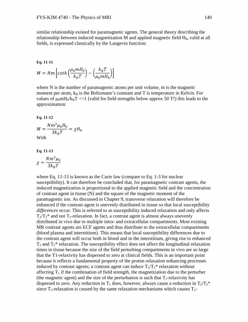
'�� ZQ[Q MTT is related to the ‘mismatch’ between perfusion and blood volume and this parameter has proved to be particularly important is cerebral stroke assessment. Figure 12-5 shows a sample case from a patient with acute stroke. The area of elevated MTT

BV BF MTT

Figure 12-5. DSC perfusion images in a patient with acute stroke. Note the elevated MTT values in the affected region (circle) representing tissue at risk of infarction due to mismatch between blood volume and blood flow (stagnant blood)


values in the right image (circle) represent tissue at risk of infarction due to severely reduced flow.

12.4. Dynamic contrast enhanced imaging Dynamic contrast enhanced (DCE) MR imaging is a collective term used to describe different methods assessing the dynamic effect of an MR contrast agent following a rapid bolus injection. DCE imaging usually referrers to dynamic imaging outside the central nervous system (i.e. not including brain perfusion imaging as discussed in the previous section). As discussed in the Contrast Agent chapter, small MW contrast agents are only intravascular agents in the CNS and will leak into the interstitial space in all other body areas. The rate at which the contrast agent diffuses from plasma to the interstitium (and eventually back to plasma) is determined both by physiological parameters (blood flow and the permeability or ‘leakiness’ of the capillary wall) as well as properties of the contrast agent (e.g. molecular size, configuration and charge).Since most DCE imaging today is performed using conventional gadolinium based extracellular fluid (ECF) agents, we will restrict the discussion to such agents. The mathematics describing the dynamic distribution of the contrast agent in vivo is referred to as kinetic modeling and for Gd-ECF agents the distribution is for most situations well described by a two-compartment model as illustrated in Figure 12-6. In a two-compartment model, the contrast agent is assumed to reside either in the plasma space or in the extravascular, extracellular space

(EES) and the flux of contrast between the two compartments is described by two transfer constants. Mathematically, this dynamic system can be described by the following differential equation:

Ktrans

kep

EESPlasma

Figure 12-6. Two-compartment representation of contrast leakage from the intravascular space to the extravascular, extracellular space (EES). The flux of contrast agent between the two compartments are described by the two tranfer-constants Ktrans and Kep.


Eq. 12-8 &�Q&( � aQ�\b��c�(� )dc�Q�(�

where Ktrans and kep are the transfer constants as defined in Figure 12-6 and Cp and Ct are the contrast agent concentrations in plasma and EES, respectively. Assuming that the initial condition is zero it can easily be shown that the solution to Eq. 12-8 is given by the following convolution integral:

Eq. 12-9

�Q�(� � aQ�\b� @ �c�� expN )dc�( ��O &�Q�

We see that, as was the case for perfusion analysis, we assume that the contrast agent concentration can be determined both in an artery (Cp) and in tissue (Ct) from the measured dynamic MR signal response. If both arterial and tissue contrast agent concentrations can be estimated (based on the assumptions described earlier) then the transfer constants can be determined using standard deconvolution mathematics. However, the plasma concentration (arterial input function) is often difficult to assess due to lack of arterial vessels in the image plane or too poor spatial resolution. In this case we can assume that the plasma concentration follows a certain time-course. If the temporal resolution is low, then Cp can be fairly well approximated by a mono-exponential function with a half-life equal to the elimination half-life of the contrast agent (around 60 minutes for renally excreted Gd-ECF agents). For higher temporal resolutions (seconds rather than minutes) Cp needs to be modeled by a bi-exponential function in order to include the initial distribution phase as well. If we model the plasma concentration as Cp=Cp(0)exp(-t/T1/2) (plasma half-life = T1/2) we then get:

Eq. 12-10

&�Q&( � aQ�\b��c,�exp e (��f )dc�Q�(�

This is a non-homogeneous equation (y’ + p(x)y=r(x)) with solution:

Eq. 12-11

�Q�(� � aQ�\b��c,��/� )dc gIJK� )dc(� IJK L (��/�Mh


If we now assume that both Cp,0 and T1/2 are constants then Ktrans and kep can be determined using standard non-linear least squares curve fitting methods from the dynamic time-course of the contrast enhancement. Why do we want to determine the transfer constants Ktrans and kep ? Because these parameters may provide important information about the ‘leakiness’ of the capillary walls, which can be altered in many pathological conditions. A sample DCE case in a patient with arthritis is shown in Figure 12-7 (see figure caption for details). Areas of increased Ktrans i.e. increased ‘leakiness’ to the contrast agent are clearly seen as hot-spots in the parametric Ktrans color map.The increase in Ktrans is here

probably due to inflammatory processes in the tissue caused by the arthritis. Many tumor types have also been shown to exhibit enhanced Ktrans value due to increased leakiness of tumor vessels formed by angiogenesis.

-10

0

10

20

30

40

50

60

70

80

0 20 40 60 80 100 120

Figure 12-7. DCE imaging in a patient with arthritis. The top image shows one of the raw T1-weighted images in the dynamic acquisition and the curves show the dynamic evolution of the contrast enhancement (in percent enhancement rel to baseline) from the two regions of interest. The color image shows the corresponding Ktrans image calculated from the dynamic curves using Eq. 12-11. Areas of increased ‘leakiness’ due to inflammatory processes are clearly seen as hot-spots in the image.

Documents

11. MR Contrast Agents - Universitetet i · PDF file11. MR Contrast Agents ... relaxation times and the distinction between T1- and T2- enhancing agents is therefore somewhat artificial