Offshoring and Sequential Production Chains: A General-Equilibrium Analysis

Philipp Harms, Jaewon Jung, and Oliver Lorz

Working Paper 14.01

This discussion paper series represents research work-in-progress and is distributed with the intention to foster discussion. The views herein solely represent those of the authors. No research paper in this series implies agreement by the Study Center Gerzensee and the Swiss National Bank, nor does it imply the policy views, nor potential policy of those institutions.

Offshoring and Sequential Production Chains:

A General-Equilibrium Analysis

Philipp Harms∗, Jaewon Jung†, and Oliver Lorz‡

This version: January 5, 2014§

Abstract

In this paper, we develop a two-sector general equilibrium trade model which

includes offshoring, sequential production, and endogenous market structures. We

analyze how relative factor endowments and various forms of globalization and tech-

nological change affect equilibrium offshoring patterns. We show that, against common

belief, a reduction in trade costs lowers the range of tasks offshored even though the

aggregate volume of offshoring may increase.

Keywords: Offshoring, sequential production, global production chain, task trade.

JEL Classification: D24, F10, F23, L23.

∗Johannes Gutenberg University Mainz, Gutenberg School of Management and Economics, Jakob-

Welder-Weg 4, 55128 Mainz, Germany.†Corresponding author. RWTH Aachen University, School of Business and Economics, Templergraben

64, 52056 Aachen, Germany. Email: Jung@wiwi.rwth-aachen.de.‡RWTH Aachen University, School of Business and Economics.§For helpful comments and suggestions on a preliminary version of this paper, we thank Frank Stähler

and participants at the ETSG 2012 Leuven conference, at the ATW 2013 Melbourne workshop, and at

seminars in Hannover, Heidelberg, Mainz, and Tuebingen.

1 Introduction

Over the past years a lot of attention has been devoted to the determinants and con-

sequences of the “second unbundling” in international trade (Baldwin 2006) — i.e., the

international fragmentation of production.1 Most analyses of this phenomenon are based

on a specific idea of the production process, according to which individual tasks can be

ordered with respect to the cost advantage of performing them abroad (including addi-

tional monitoring and communication costs resulting from foreign production), and the

decision to offshore a certain task depends on the production and offshoring costs for that

particular task. Some recent contributions, however, explicitly consider the fact that in

many cases the production process is sequential — i.e., individual steps follow a predeter-

mined sequence that cannot be modified at will.2

Relative costs of performing individual steps not necessarily increase or decline mono-

tonically along the production path. Instead, a foreign country may have a cost advantage

for some particular segment of the production process whereas preceding and following

segments can be performed at lower costs in the domestic country. If such a situation is

combined with transport costs of shipping intermediate goods across borders, firms may

find it disadvantageous to offshore certain steps even if they could be performed at much

lower costs abroad. The reason is that the domestic country may have a cost advantage

with respect to adjacent steps, and the costs of shifting back and forth intermediate goods

may more than eat up potential cost savings from fragmenting the production process.

Such a constellation may have important implications for observed offshoring patterns.

For example, it may explain why certain production processes are less fragmented in-

ternationally as one might expect — given the large international discrepancies in factor

prices.

Baldwin and Venables (2013) as well as Harms et al. (2012) have shown how such

1A non-exhaustive list of important contributions to this literature includes Jones and Kierzkowski

(1990), Feenstra and Hanson (1996), Kohler (2004), and Grossman and Rossi-Hansberg (2008).2See, e.g., Antras and Chor (2013), Baldwin and Venables (2013), Costinot et al. (2012, 2013), Harms et

al. (2012), or Kim and Shin (2012). Important earlier approaches are Dixit and Grossman (1982), Sanyal

(1983), Yi (2003), and Barba Navaretti and Venables (2004). Fally (2012), Antras and Chor (2013), and

Antras et al. (2012) provide empirical measures to characterize sequential production processes.

2

insights regarding the offshoring decision of individual firms can be obtained already from

simple partial equilibrium models in which factor prices are exogenous. However, to arrive

at conclusions about the entire economy, we need to account for the influence of firms’

offshoring decisions on factor prices at home and abroad, and we have to consider the

repercussions of induced factor price changes on firms’ optimal behavior — i.e., we need

to model offshoring in a general equilibrium framework. This is what the current paper

does.

Baldwin and Venables (2013) model firms’ offshoring decisions for different configura-

tions of production processes — “snakes” and “spiders” — with spiders reflecting a situation

in which different intermediate inputs may be simultaneously produced in different coun-

tries to be eventually assembled at a central location, and snakes capturing the notion

of sequentiality outlined in the introduction. Using these alternative frameworks, they

analyze the consequences of exogenous variations in production costs and offshoring costs,

including costs of shipping intermediate goods across borders. Highlighting the “tension

between comparative costs creating the incentive to unbundle, and co-location or agglom-

eration forces binding stages of production together”(Baldwin and Venables 2013: 246),

which is also characteristic for our setup, they show that a decrease in shipping costs may

result in an overshooting of the overall offshoring pattern: Production stages may first be

shifted abroad to take advantage of co-location and then return to the domestic country

as shipping costs further decrease. In Harms et al. (2012), relative costs fluctuate sym-

metrically along the production process, allowing a deeper analysis of the technological

factors that influence the offshoring decision. In addition to shipping costs, Harms et al.

(2012) consider communication and supervision costs caused by offshoring activities as

well as the variability of these costs between tasks, or the total length of the production

chain.

The current paper starts from a similar symmetric specification of a production-

“snake”and places this in a general equilibrium context. We present a two-country (North-

South) model in which firms whose production is entirely domestic may coexist with mul-

tinational firms who decide on the international distribution of production. Production is

based on a rigid sequence of individual steps, and the foreign cost advantage evolves in

a non-monotonic fashion along the production chain: some steps are cheaper to perform

3

in the South, some are cheaper to perform in the North, and so on. Finally, every step

requires the presence of the unfinished intermediate good, and shifting intermediate goods

across borders is associated with transport costs. Wages and prices in both economies

are endogenous, and the increasing demand for labor that is generated by accelerating

North-South offshoring may eventually result in wage increases that make offshoring less

attractive. Using this framework and employing numerical simulations, we explore how

changes in transport costs, relative productivities and properties of the production process

affect the number of firms whose entire production takes place in the domestic economy,

the number of firms that decide to fragment their production process between North and

South, and the number of firms that relocate (almost) the entire production process to

the foreign country.

In another related approach, Costinot et al. (2012, 2013) use a general-equilibrium

model with multiple countries to analyze how a countries’ productivity — as reflected by

its propensity to commit mistakes — determines the stages of production it attracts. These

authors also emphasize the concept of sequentiality, i.e., the idea that the order in which

tasks have to be performed is exogenously determined. Moreover, the transport costs in

our model play a role that is somewhat similar to the “coordination costs” in Costinot et

al. (2013: 111), with a decrease in these costs inducing a non-monontonic adjustment of

the overall volume of offshoring. However, we deviate from the monotonicity assumption

in Costinot et al. (2012, 2013), which stipulates that countries can be ordered by their

relative productivities. Conversely, we model a two-country world in which the relative

cost advantage of the North fluctuates non-monotonically along the production chain.

This enables us to analyze how specific properties of industry-specific production processes

affect the volume of offshoring and relative factor prices across countries.

4

2 The Model

2.1 Preferences

There are two countries (or regions), North and South, with an asterisk denoting South-

specific variables. Consumers in both countries have Cobb-Douglas preferences over two

consumption goods, and . The sector produces a continuum of differentiated

varieties, whereas goods from the sector are homogeneous. Household preferences are

= 1− 0 1 and (1)

=

∙Z∈

()

¸ 1

0 1 (2)

The index denotes individual varieties, and = 1(1−) is the elasticity of substitutionbetween these varieties. Maximizing utility for a given income level () yields the

following demand system:

() =

µ

()

¶

(3)

=

∙Z∈

()1−¸ 11−

= and = (1− ) (4)

2.2 Technologies and Production Modes

Each country is endowed with fixed quantities of labor (in efficiency units) and a fixed

composite factor . As Markusen and Venables (1998), we assume that labor can be

employed in both sectors, whereas the fixed composite factor, which may be land or a

natural resource, is specific to industry (see also Markusen, 2002). Good is produced

in both countries by a competitive industry and can be freely traded. Production of

employs and according to a CES-technology

=£

+

¤ 1 0 1 (5)

from which profit maximization yields the following demand for the two factors of pro-

duction:

=

³

´ and =

³

´ (6)

5

The term = 1(1− ) stands for the elasticity of substitution between the two factors and , and and denote factor prices, respectively. If good is produced, perfect

competition implies that

=£ 1− +

1−

¤ 11− (7)

We choose good as our numeraire throughout the paper, and from free trade in and

product homogeneity we have = ∗ = 1.

Varieties of good can only be produced by firms whose headquarters are located

in the North. While we do not explicitly model research and development, this assump-

tion can be rationalized by arguing that only Northern firms are able to develop and use

the blueprints necessary for production. Firms in sector act under monopolistic com-

petition, and each firm has to spend fixed costs in addition to the variable production

costs.

The production process of any variety () consists of a continuum of tasks, indexed

by , ranging from 0 to 1. These tasks have to be performed following a strict sequence,

i.e., they cannot be re-arranged at will. This property of a sequential production process

is important since some of these tasks may be offshored to exploit international cost

differences, and these cost differences may vary along the production process in a non-

monotonic fashion. A firm producing a given variety of good may choose between two

available production modes: domestic () and multinational (). While domestic firms

perform the entire production process in the North, multinational firms can offshore some

of the tasks to the South. The goal of our analysis is to determine the share of good-

producers that decides to take advantage of the possibility to produce internationally and

to derive the amount of offshoring chosen by these firms.

Each task involves a given quantity of labor. The labor coefficients () or ()

denote the efficiency units of labor that are necessary for a domestic () or multinational

() firm to perform task in the North.3 For simplicity, we assume that () = and

() = for all , i.e., input coefficients in the North do not differ across tasks. Being a

3By contrast to this assumption of fixed labor coefficients, Jung and Mercenier (2008), who analyze

skill/technology upgrading effects of globalization, employ a heterogeneous workers framework in which a

worker’s productivity is determined endogenously by his own talent and the technology he uses.

6

multinational firm may come with a higher labor productivity in the North, i.e., ≤ .

Input coefficients ∗() of performing a task in the South possibly differ from , and —

more importantly — these coefficients vary across tasks. For example, some tasks benefit

more strongly from a better educated workforce or a better production infrastructure in

the North, implying a lower labor coefficient in the North than in the South. Other tasks

may be less sophisticated such that the effective labor input for these tasks may be lower

in the South than in the North. In addition, offshoring firms possibly have to employ

additional labor to monitor tasks performed in the South or to communicate with the

headquarter in the North, and these monitoring and communication requirements may

also vary across tasks. Summing up, there may be tasks which — given wages and ∗

in the North and the South respectively — are cheaper to perform domestically and tasks

which are cheaper to perform abroad. This is represented by Figure 1, which juxtaposes

the (constant) costs per task if these tasks are performed by a Northern domestic

firm, the (constant) costs if they are performed domestically by a multinational firm,

and the varying costs ∗∗() if these tasks are offshored to the South.

Multinational firms have to adjust to the fact that, at given wages, some tasks that are

cheaper to perform in the South may be “surrounded” by tasks for which the North has

a cost advantage (and vice versa). In Figure 1, the tasks ∈ [1 2] and ∈ [3 4] wouldbe performed at lower cost if they were offshored to the South by Northern multinational

firms. Conversely, all tasks ∈ [0 1], ∈ [2 3] and ∈ [4 1] would be cheaper to performdomestically. To simplify the analysis, we assume that the first and the last task are tied

to being performed in the North.

7

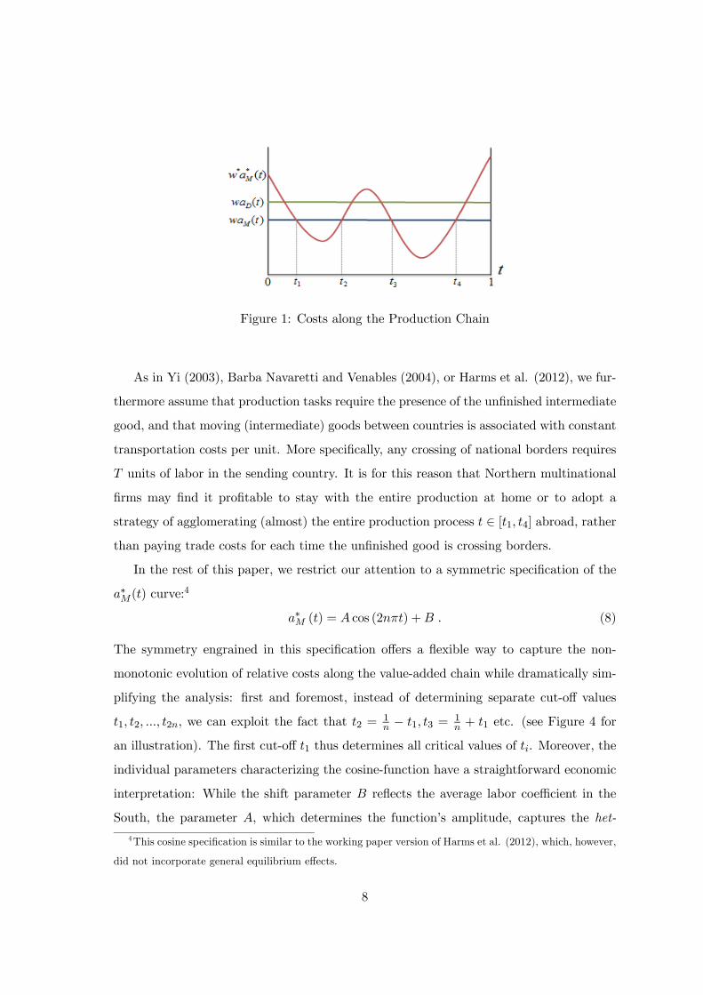
Figure 1: Costs along the Production Chain

As in Yi (2003), Barba Navaretti and Venables (2004), or Harms et al. (2012), we fur-

thermore assume that production tasks require the presence of the unfinished intermediate

good, and that moving (intermediate) goods between countries is associated with constant

transportation costs per unit. More specifically, any crossing of national borders requires

units of labor in the sending country. It is for this reason that Northern multinational

firms may find it profitable to stay with the entire production at home or to adopt a

strategy of agglomerating (almost) the entire production process ∈ [1 4] abroad, ratherthan paying trade costs for each time the unfinished good is crossing borders.

In the rest of this paper, we restrict our attention to a symmetric specification of the

∗() curve:4

∗ () = cos (2) + (8)

The symmetry engrained in this specification offers a flexible way to capture the non-

monotonic evolution of relative costs along the value-added chain while dramatically sim-

plifying the analysis: first and foremost, instead of determining separate cut-off values

1 2 2, we can exploit the fact that 2 =1− 1 3 =

1+ 1 etc. (see Figure 4 for

an illustration). The first cut-off 1 thus determines all critical values of . Moreover, the

individual parameters characterizing the cosine-function have a straightforward economic

interpretation: While the shift parameter reflects the average labor coefficient in the

South, the parameter , which determines the function’s amplitude, captures the het-

4This cosine specification is similar to the working paper version of Harms et al. (2012), which, however,

did not incorporate general equilibrium effects.

8

erogeneity of task-specific input requirements across countries. The variable ( ∈ N+)measures the number of “cycles” that ∗() completes between = 0 and = 1. We

argue that production processes that are characterized by a higher number of cycles — i.e.,

a larger — are more sophisticated, exhibiting more variability in terms of cost differences.

To keep the analysis interesting, we assume that foreign production costs fluctuate around

domestic costs more than once ( ≥ 2).Offshoring with positive production volumes in both countries can only occur if each

country has a cost advantage for some tasks. Technically, this requires that the ∗∗()

curve in Figure 1 intersects the line at least once. Therefore, a necessary condition

for international production sharing in our paper is

−

∗

+

(9)

Due to the symmetric specification of the ∗() function, we may distinguish three

firm-types ∈ © ª: domestic firms (domestic production, D), multinational

firms that fragment their production chain (fragmentation, ), or multinational firms

that perform most tasks in the South (production abroad, ).5 Fragmented multination-

als offshore all segments that are cheaper to perform in the South, i.e., all tasks between

and +1 ( = 1 3 2 − 2), and produce all other segments at home. Productionabroad firms offshore the entire segment between 1 and 2, and produce only the first

segment between 0 and 1 and the last segment between 2 and 1 at home.

2.3 Costs and Prices

Defining for future use the dummy term ( = 0 if = , and = 1 if = ),

marginal costs of firm type are given by the following expression:

= + ∗∗ (10)

5The fact that there are only three firm types in equilibrium is due to our symmetric parametrization

of ∗ ().

9

The variables and ∗ stand for the labor input at home and abroad per unit of output

of a representative type- firm, given by

= (11)

= 2 1 + (12)

= 2 1 + (13)

∗ =

Z 1−1

1

( cos(2) +) +

= [1− 21]−

sin (21) + and (14)

∗ =

Z 1

0

( cos(2) +) − 2Z 1

0

( cos(2) +) +

= [1− 21]−

sin(21) + (15)

Note that with cycles, fragmented firms ( ) have 2+1 sequential production stages,

and transport costs of times in each country, while production abroad firms ()

have 3 sequential production stages and transport costs of in each country.

We assume that exporting final -goods to the South is associated with iceberg trade

costs 1 per unit. Using this information as well as equations (3) and (4), we can write

the demand faced by a representative firm of type as

=

µ

¶

and ∗ =

µ ∗

¶

∗ (16)

The price indices for the sector in the North and the South are given by

=

⎡⎣X

1−

⎤⎦ 11−

and ∗ =

⎡⎣X

()1−

⎤⎦ 11−

(17)

where stands for the mass of firms of each firm-type.

If type- firms in sector produce a strictly positive quantity ( 0), they charge a

constant mark-up rate over their marginal costs:

=

− 1 (18)

We assume that all active firms have to incur fixed costs that take the form of unsold

final goods, i.e., they amount to a multiple of marginal costs , with 0. Consistent

10

with evidence we assume .6 Free entry ensures zero profits, such that

revenues cover total costs:

1

≤ (19)

where 0 if the respective condition holds with equality, and = 0 otherwise. With

positive production, we can combine (18) with (19) to derive production of a firm of type

in equilibrium:

= ( − 1) (20)

3 Equilibrium

3.1 Definition

An equilibrium is defined by an optimal cutoff value 1, a vector of wages as well as prices

and quantities in the and sectors, and an industrial structure ( ) such

that () firms of a given type in the -sector set profit-maximizing prices,

() no firm has an incentive to change its production mode,

()multinational firms of a given type (, ) choose the optimal pattern of offshoring,

i.e., the cutoff value 1,

() free entry results in zero-profits of all active firms in equilibrium,

() in the -sector, factor prices reflect their marginal products,

() goods and factor markets are cleared.

3.2 Cutoff Task

The optimal cutoff task 1 is implicitly determined by the following condition:

= ∗∗(1) (21)

Using (8), we can obtain 1 as

1 =1

2arccos

µ∗ −

¶ (22)

6As is common in the literature, we assume that the fixed organizational and set-up costs are higher

abroad than domestically. Consequently, they increase in the range of activities performed abroad, implying

.

11

That is, the range of offshored tasks depends on the domestic labor coefficient , the

average foreign coefficient , and on the wage ∗ in the North relative to the South.

Not surprisingly, an increase in ∗ ceteris paribus lowers 1, i.e.,

1

(∗)= −

2

r1−

³∗−

´2 0

The economic intuition behind this result is straightforward: as the domestic wage relative

to the foreign wage increases, firms have an incentive to perform a smaller share of the

production process at home and a larger share abroad. In a similar fashion, we may

determine the influence of the variables determining average costs, and , as well as

the heterogeneity parameters and .

3.3 Market Clearing

Labor market equilibrium requires

= + ( + )+

( + ) + ( + ) and (23)

∗ =∗ + ∗ ( + ) + ∗( + ) (24)

where ( + ) is the fixed and variable labor input required by domestic firms to

produce units of output, ( + ) the fixed and variable labor input used by

fragmenting multinationals in the North etc. For the market of the fixed composite factor

to be in equilibrium we need

= and ∗ = ∗ (25)

The equilibrium conditions on the factor markets determine , , ∗ and ∗, respectively,

and final-goods’ market equilibrium imposes that

= + ∗ as well as (26)

+∗ = + ∗ (27)

Finally, incomes depend on factor prices and (fixed) factor supplies:

= + and ∗ = ∗∗ + ∗∗ (28)

12

3.4 Production Regimes

In what follows, we distinguish between equilibria in which all -sector firms choose

the same production mode and equilibria in which firms with different production modes

coexist. We will refer to these constellations as production regimes: a domestic production

regime is characterized by = = 0 and 0, a mixed domestic/fragmented

regime is characterized by = 0 and 0 0, etc.

In a regime in which different production modes and coexist, equation (20) implies

= . Since it follows from (16) and (18) that = ()− and =

, we obtain

=

µ

¶−1 (29)

Unit costs and are given by (10) combined with (11) — (15). For further reference

we define

=

µ

¶−1and =

µ

¶−1(30)

as the fixed cost advantage of producing domestically compared to fragmented production

or production abroad, respectively. Since , we have 1.

With these definitions, we can characterize conditions for the different production re-

gimes. For example, if = , domestic and fragmented production coexist. If

= , fragmented production and production abroad coexist. If, however,

and , all firms choose domestic production. From (10) to

(15), and combining (8) and (21) we have

= (31)

= 2 1 + +

cos(21) +

∙¡1− 21

¢−

sin¡21

¢+

¸ (32)

= 2 1 + +

cos(21) +

∙¡1− 21

¢−

sin¡21

¢+

¸ (33)

Figure 2 depicts marginal costs (relative to and ) as a function of the optimal cutoff

value 1.7

7From taking the derivatives of (32) and (33) and from 1 1, it can be shown that

( ) 1 () 1, as depicted in Figure 2.

13

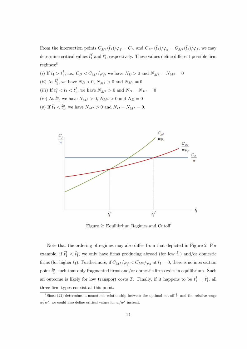
From the intersection points (1) = and (1) = (1) , we may

determine critical values 1 and

1, respectively. These values define different possible firm

regimes:8

() If 1 1 , i.e., , we have 0 and = = 0

() At 1 , we have 0, 0 and = 0

() If 1 1 1 , we have 0 and = = 0

() At 1, we have 0, 0 and = 0

() If 1 1, we have 0 and = = 0.

Figure 2: Equilibrium Regimes and Cutoff

Note that the ordering of regimes may also differ from that depicted in Figure 2. For

example, if 1 1, we only have firms producing abroad (for low 1) and/or domestic

firms (for higher 1). Furthermore, if at 1 = 0, there is no intersection

point 1, such that only fragmented firms and/or domestic firms exist in equilibrium. Such

an outcome is likely for low transport costs . Finally, if it happens to be 1 = 1, all

three firm types coexist at this point.

8Since (22) determines a monotonic relationship between the optimal cut-off 1 and the relative wage

∗, we could also define critical values for ∗ instead.

14

3.5 Model Solution

This section illustrates the necessary steps to determine the equilibrium values of the

model variables in a given production regime. As a starting point, we consider the most

straightforward case, the domestic production regime in which there is no offshoring to

the South. From equations (5) and (6) we can derive

∗=

⎛⎝

³

´+

³∗∗

´+

⎞⎠1−

(34)

This shows that the relative wage decreases in domestic employment in the -sector ( )

and increases in foreign employment in that sector (∗ ). Given the diminishing marginal

product of labor in that sector, this result is not surprising. In a production regime in which

all firms of the -sector produce only domestically, we have = = 0. Using this

property, the firm-level output (20) as well as the domestic labor-market clearing condition

(23) yields

= − (35)

Purely domestic production also implies ∗ = ∗. To compute the number of firms in

equilibrium (), we substitute the supply equation (20) as well as the demand and

pricing equations (16) and (17) into the goods market equilibrium condition (26) . This

results in

=

µ + ∗

( − 1)

¶−1

(36)

Combining (4), (6), (10), (11), (17), (18), and (28) yields

= 1

−1

( − 1)

Ã+

µ

¶ 1

!and (37)

∗ = 1

−1

( − 1)

µ∗

¶Ã∗ +

µ∗

∗

¶ 1

∗!

(38)

Equations (36), (37) and (38) imply

= Λ

"+

µ

¶ 1

+

µ∗

¶Ã∗ +

µ∗

∗

¶ 1

∗!#

(39)

where Λ ≡

. Combining (35) and (39) yields as a function increasing in the

relative wage ∗. This relationship is driven by the fact that an increasing domestic

15

wage raises costs in the -sector and reduces the number of firms . This, in turn, raises

the supply of labor in the -sector. Together with (34), which establishes a negative rela-

tionship between and ∗, this uniquely determines the relative wage in equilibrium.

Once we have identified the equilibrium value of ∗ for a given parameter constellation,

we have to check whether it is indeed the case that and .

The analysis of the two other regimes that are characterized by a single firm type

proceeds in a similar fashion. Compared to the domestic-production regime, the only

complication that arises is that we cannot set ∗ = ∗ and that the cost function of

domestic firms in the sector involves the optimal threshold value 1 (see (12) — (15)).

However, equation (22) characterizes 1 as a function of the relative wage ∗, which

closes the model.

In a production regime with two firm types we have to determine an additional en-

dogenous variable (e.g., , if domestic and fragmented firms coexist). This can be

achieved by using the free-entry condition (29) as an additional equation. In the mixed

domestic/fragmented regime, for example, we have to determine both and , and

we can use the additional condition = , combined with (10), (11), (12), (13)

and (22) to uniquely determine the relative wage ∗. Again, once we have computed

prices and quantities for such a regime, we have to make sure that no firm has an incentive

to deviate from its choice of production mode. The analysis of other mixed production

regimes proceeds in the same fashion.

3.6 Comparative Static Analysis

Given the complexity of our model, it is hard to derive general qualitative comparative-

static results. However, for the case of a mixed production regime, we can use the free-

entry condition (29) and the formula for the optimal cutoff value (22) to analyze how

exogenous variations of parameter values affect the relative wage and the intensive margin

of offshoring. We specify this for the case of a regime in which domestic and fragmented

production coexist. As mentioned in the previous section, this requires = .

16

Inserting for and yields + ∗

∗ = , or

∗=

∗

−

=£1− 21

¤− sin(21) +

− 2 1 − (40)

This condition establishes a relationship between the optimal cutoff value 1 and the

relative wage ∗. Taking the derivative of (40) with respect to 1 yields

(∗)1

=−2∗(1)

¡ −

¢+ 2∗

¡ − ∗

¢2=−2∗

¡ −

¢+ 2∗

¡ − ∗

¢2=−2∗

+ 2∗¡

− ∗

¢2= 0

A marginal change in the optimal cutoff does not influence the relative wage. This result

is an application of the envelope theorem: a change in ∗ would be necessary if a

variation of 1 affected firms’ marginal costs at the given relative wage. However, since 1

is chosen to minimize the marginal costs of fragmented firms, this effect disappears.

Figure 3 depicts the “free-entry” (FE) relationship (40) and the “optimal cutoff” (OC)

condition (22). As we have seen in section 3.2, the optimal cutoff 1 decreases in the

relative wage ∗. The point of intersection defines the unique cut-off value 1 and the

relative wage ∗ which prevail in a regime in which domestic and fragmented production

coexist. For a mixed regime with domestic firms and firms producing abroad, we can set

up a similar figure as the free entry condition is also horizontal in this case.

17

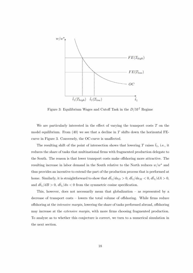
Figure 3: Equilibrium Wages and Cutoff Task in the Regime

We are particularly interested in the effect of varying the transport costs on the

model equilibrium. From (40) we see that a decline in shifts down the horizontal FE-

curve in Figure 3. Conversely, the OC-curve is unaffected.

The resulting shift of the point of intersection shows that lowering raises 1, i.e., it

reduces the share of tasks that multinational firms with fragmented production delegate to

the South. The reason is that lower transport costs make offshoring more attractive. The

resulting increase in labor demand in the South relative to the North reduces ∗ and

thus provides an incentive to extend the part of the production process that is performed at

home. Similarly, it is straightforward to show that 1 0, 1 0, 1 0,

and 1 0, 1 0 from the symmetric cosine specification.

This, however, does not necessarily mean that globalization — as represented by a

decrease of transport costs — lowers the total volume of offshoring. While firms reduce

offshoring at the intensive margin, lowering the share of tasks performed abroad, offshoring

may increase at the extensive margin, with more firms choosing fragmented production.

To analyze as to whether this conjecture is correct, we turn to a numerical simulation in

the next section.

18

4 A Numerical Appraisal

In this section, we perform a numerical exercise to further understand the forces that

determine the extent of offshoring. As outlined above, our model allows for two dimensions

along which the extent of offshoring changes as exogenous parameters vary: first, the share

of the production process that is performed abroad for a given firm-type may increase or

decrease (the intensive margin). Second, the number of firms of a certain type may vary

(the extensive margin). We analyze how offshoring reacts at the extensive and at the

intensive margin to a decline in transport costs, changes in relative productivities and

other properties of the production process.

4.1 Calibration

The two countries are scaled so that initially about half of the domestic consumption of

good is imported from the South, while goods are produced only by Northern firms

and exported to the South. With preference parameter = 05, the North is endowed

with one third of the world’s and two thirds of the world’s , while the South is endowed

with the rest.9 In industry , we set = 4 and = 2 as benchmark values for the

substitution elasticity and the number of cycles of ∗(). We choose somewhat arbitrarily

— but within the ranges consistent with our theoretical constraints — the fixed costs and

the trade cost of each border crossing of intermediate inputs: = 10; = 13;

= 15; = 02. With this functional form and parameter values, we calibrate the key

technological parameters — , , and —, so that initially about half of the total

is produced by -type firms and the other half by -type firms. Figure 4 displays the

three calibrated technologies and the resulting cutoff tasks.10

9Note that our framework adopts elements from both the Ricardian and the Heckscher-Ohlin framework,

i.e., trade is driven by differences in factor endowments and by technological differences. While our

assumption that the North is relatively abundant in labor may seem unjustified at first glance, note that

reflects effective labor supply, which is determined by both demographic and technological factors.10Appendix A reports the benchmark parameter and equilibrium variable values.

19

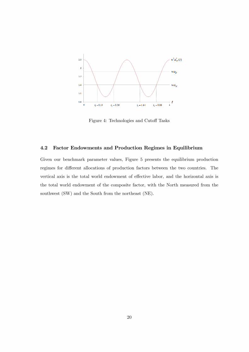
Figure 4: Technologies and Cutoff Tasks

4.2 Factor Endowments and Production Regimes in Equilibrium

Given our benchmark parameter values, Figure 5 presents the equilibrium production

regimes for different allocations of production factors between the two countries. The

vertical axis is the total world endowment of effective labor, and the horizontal axis is

the total world endowment of the composite factor, with the North measured from the

southwest (SW) and the South from the northeast (NE).

20

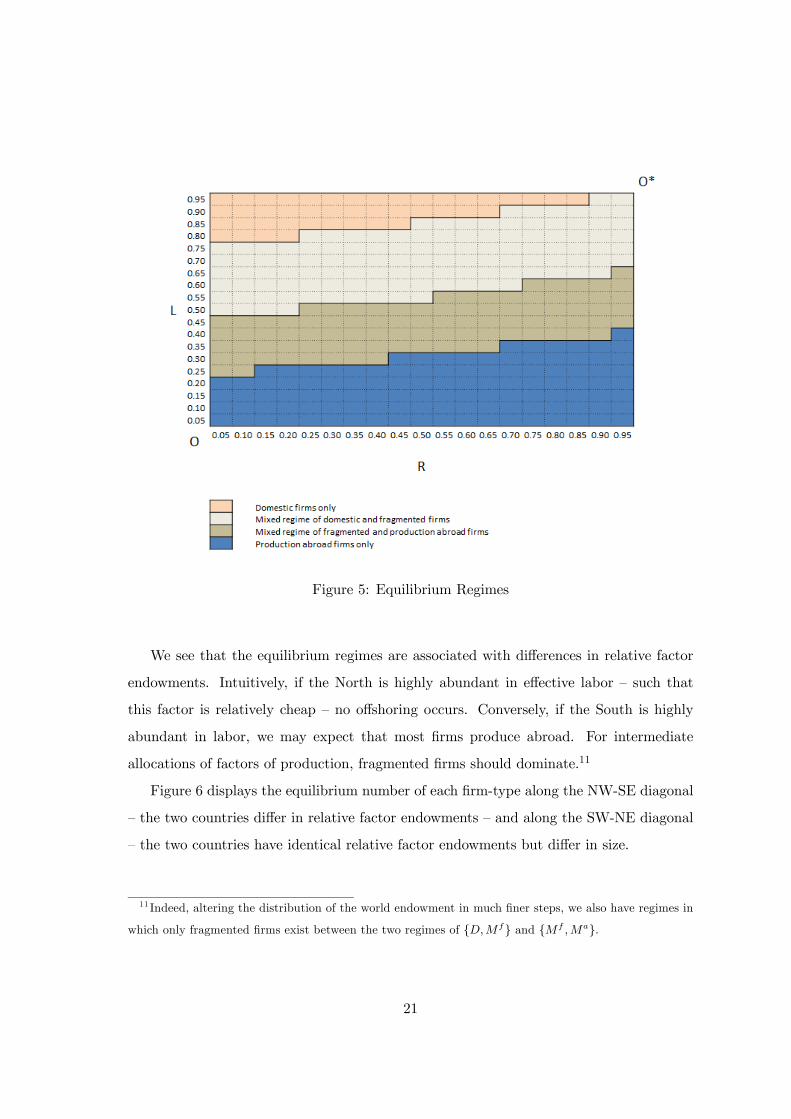
Figure 5: Equilibrium Regimes

We see that the equilibrium regimes are associated with differences in relative factor

endowments. Intuitively, if the North is highly abundant in effective labor — such that

this factor is relatively cheap — no offshoring occurs. Conversely, if the South is highly

abundant in labor, we may expect that most firms produce abroad. For intermediate

allocations of factors of production, fragmented firms should dominate.11

Figure 6 displays the equilibrium number of each firm-type along the NW-SE diagonal

— the two countries differ in relative factor endowments — and along the SW-NE diagonal

— the two countries have identical relative factor endowments but differ in size.

11 Indeed, altering the distribution of the world endowment in much finer steps, we also have regimes in

which only fragmented firms exist between the two regimes of {} and { }.

21

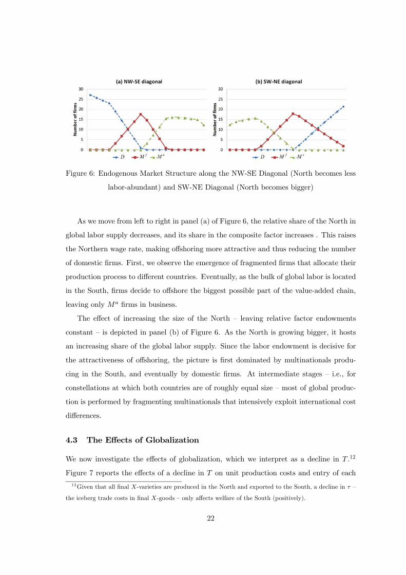
Figure 6: Endogenous Market Structure along the NW-SE Diagonal (North becomes less

labor-abundant) and SW-NE Diagonal (North becomes bigger)

As we move from left to right in panel (a) of Figure 6, the relative share of the North in

global labor supply decreases, and its share in the composite factor increases . This raises

the Northern wage rate, making offshoring more attractive and thus reducing the number

of domestic firms. First, we observe the emergence of fragmented firms that allocate their

production process to different countries. Eventually, as the bulk of global labor is located

in the South, firms decide to offshore the biggest possible part of the value-added chain,

leaving only firms in business.

The effect of increasing the size of the North — leaving relative factor endowments

constant — is depicted in panel (b) of Figure 6. As the North is growing bigger, it hosts

an increasing share of the global labor supply. Since the labor endowment is decisive for

the attractiveness of offshoring, the picture is first dominated by multinationals produ-

cing in the South, and eventually by domestic firms. At intermediate stages — i.e., for

constellations at which both countries are of roughly equal size — most of global produc-

tion is performed by fragmenting multinationals that intensively exploit international cost

differences.

4.3 The Effects of Globalization

We now investigate the effects of globalization, which we interpret as a decline in .12

Figure 7 reports the effects of a decline in on unit production costs and entry of each

12Given that all final -varieties are produced in the North and exported to the South, a decline in —

the iceberg trade costs in final -goods — only affects welfare of the South (positively).

22

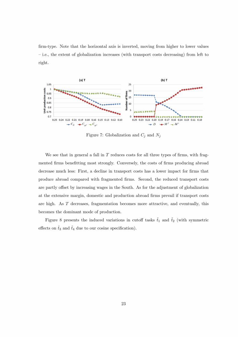
firm-type. Note that the horizontal axis is inverted, moving from higher to lower values

— i.e., the extent of globalization increases (with transport costs decreasing) from left to

right.

Figure 7: Globalization and and

We see that in general a fall in reduces costs for all three types of firms, with frag-

mented firms benefitting most strongly. Conversely, the costs of firms producing abroad

decrease much less: First, a decline in transport costs has a lower impact for firms that

produce abroad compared with fragmented firms. Second, the reduced transport costs

are partly offset by increasing wages in the South. As for the adjustment of globalization

at the extensive margin, domestic and production abroad firms prevail if transport costs

are high. As decreases, fragmentation becomes more attractive, and eventually, this

becomes the dominant mode of production.

Figure 8 presents the induced variations in cutoff tasks 1 and 2 (with symmetric

effects on 3 and 4 due to our cosine specification).

23

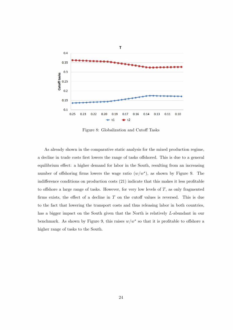
Figure 8: Globalization and Cutoff Tasks

As already shown in the comparative static analysis for the mixed production regime,

a decline in trade costs first lowers the range of tasks offshored. This is due to a general

equilibrium effect: a higher demand for labor in the South, resulting from an increasing

number of offshoring firms lowers the wage ratio (∗), as shown by Figure 9. The

indifference conditions on production costs (21) indicate that this makes it less profitable

to offshore a large range of tasks. However, for very low levels of , as only fragmented

firms exists, the effect of a decline in on the cutoff values is reversed. This is due

to the fact that lowering the transport costs and thus releasing labor in both countries,

has a bigger impact on the South given that the North is relatively -abundant in our

benchmark. As shown by Figure 9, this raises ∗ so that it is profitable to offshore a

higher range of tasks to the South.

24

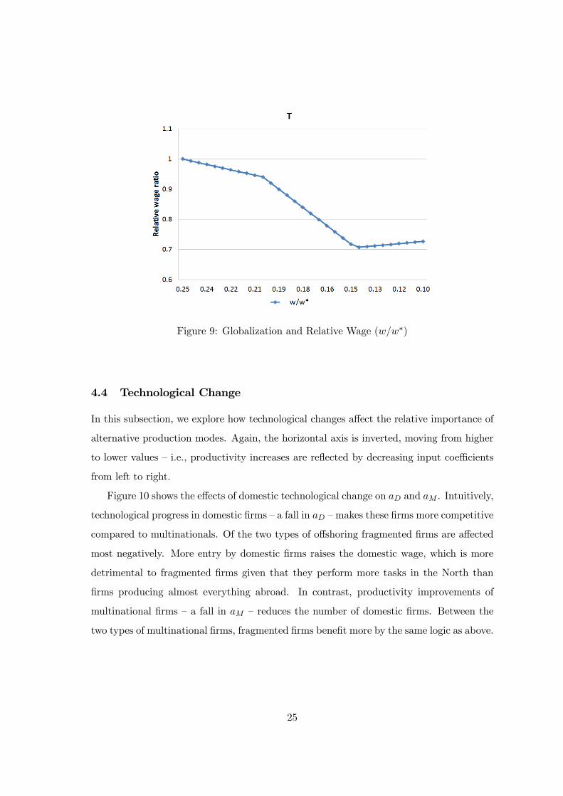
Figure 9: Globalization and Relative Wage (∗)

4.4 Technological Change

In this subsection, we explore how technological changes affect the relative importance of

alternative production modes. Again, the horizontal axis is inverted, moving from higher

to lower values — i.e., productivity increases are reflected by decreasing input coefficients

from left to right.

Figure 10 shows the effects of domestic technological change on and . Intuitively,

technological progress in domestic firms — a fall in — makes these firms more competitive

compared to multinationals. Of the two types of offshoring fragmented firms are affected

most negatively. More entry by domestic firms raises the domestic wage, which is more

detrimental to fragmented firms given that they perform more tasks in the North than

firms producing almost everything abroad. In contrast, productivity improvements of

multinational firms — a fall in — reduces the number of domestic firms. Between the

two types of multinational firms, fragmented firms benefit more by the same logic as above.

25

Figure 10: Technological Change on and

Figure 11 focuses on the South and presents the effects of varying the parameters and

. Recall that raising increases the amplitude of the ∗() function, representing greater

cost differences between different tasks in the production chain. Conversely, reducing

implies a decline in the cost advantage of producing in the South for tasks ∈ £1 2¤ and£3 4

¤. This makes fragmentation less attractive, and eventually, only domestic firms and

production abroad firms prevail. A similar pattern emerges if — i.e., the average costs

associated with producing abroad — increases: in this case, the number of firms choosing

any type of offshoring declines.

Figure 11: Technological Change on and

Finally, Figure 12 displays the effect of an increase in the number of cycles () on the

relative importance of alternative production modes.

26

Figure 12: Increase in Sophistication of the Sequential Production Chain

Increasing the sophistication of the production process — as reflected by a more complex

structure of cost differences along the value-added chain — has similar effects as an increase

in . Given that fragmented offshoring requires transportation costs of -times in each

country, raising reduces while the number of domestic firms increases.

5 Summary and Conclusion

In this paper, we have analyzed the extent of offshoring in a two-country general equilib-

rium model that is based on three crucial assumptions: First, firms’ production process

follows a rigid structure that defines the sequence of production steps. Second, domestic

and foreign relative productivities vary in a non-monotonic fashion along the produc-

tion chain. Third, each task requires the presence of an unfinished intermediate good

whose transportation across borders is costly. We believe that these assumptions are

quite plausible, e.g., characterizing production processes in the automotive industry. As a

consequence, some firms may be reluctant to offshore individual production steps, even if

performing them abroad would be associated with cost advantages: the reason is that ad-

jacent tasks may be cheaper to perform in the domestic economy and that high transport

27

costs do not justify shifting the unfinished good abroad and back home.

Using this basic structure and setting up a simple general equilibrium model along

these lines, we have analyzed the influence of technological progress and globalization

— interpreted as a variation in border crossing costs — on the volume of offshoring at

the extensive and the intensive margin. As relative production costs vary, firms adjust

the share of tasks they perform abroad (the intensive margin), and the number of firms

that fragments its production process or produces entirely abroad changes (the extensive

margin). Both adjustments may affect relative wages at home and abroad, which can

reinforce or dampen the initial impulse. We have shown that globalization in the form

of declining transport costs may have different effects on offshoring at the extensive and

intensive margin. Our analysis suggests a decrease of offshoring at the intensive margin —

i.e., firms offshore a smaller part of the entire production process — but an increase in the

number of firms that perform at least some tasks abroad.

We believe that the simplicity of our model — in particular, the symmetry of the

∗ function — has allowed us to derive some novel results, which are likely to carry

over into a more general environment. The challenge ahead is, of course, to expand the

framework to accommodate additional features of reality. The second challenge is to gauge

the relative importance of sequential production processes for the economy as a whole. Our

contribution rested on the assumption that all firms have to cope with a rigid sequence of

production steps. This may be as unrealistic as the notion that production processes can

be re-arranged freely by every firm. We believe that characterizing real-world production

processes in terms of “sequentality” holds ample promise for future research.

28

References

[1] Antras, P. and D. Chor (2013), Organizing the Global Value Chain, Econometrica,

forthcoming.

[2] Antras, P., D. Chor, T. Fally, and R. Hillberry (2012), Measuring the Upstreamness of

Production and Trade Flows, American Economic Review: Papers & Proceedings

102: 412—441.

[3] Baldwin, R., 2006, Globalisation: The Great Unbundling(s), Paper for the Finnish

Prime Minister’s Office.

[4] Baldwin, R. and A. Venables 2013, Spiders and Snakes: Offshoring and Agglomeration

in the Global Economy, Journal of International Economics 90: 245—254.

[5] Barba Navaretti, G. and A. J. Venables, 2004, Multinational Firms in the World

Economy, Princeton University Press.

[6] Costinot, A., J. Vogel, and S. Wang, 2012, Global Supply Chains andWage Inequality,

American Economic Review, Papers & Proceedings 102: 396—401.

[7] Costinot, A., J. Vogel, and S. Wang, 2013, An Elementary Theory of Global Supply

Chains, Review of Economic Studies 80: 109—144..

[8] Dixit, A. K. and G. M. Grossman, 1982, Trade and Protection with Multistage Pro-

duction, Review of Economic Studies 49: 583—594.

[9] Fally, T. 2012, Production Staging: Measurement and Facts, mimeo.

[10] Feenstra, R. C. and G. H. Hanson, 1996, Globalization, Outsourcing, and Wage In-

equality, American Economic Review, Papers & Proceedings 82: 240—245.

[11] Grossman, G. M. and E. Rossi-Hansberg, 2008, Trading tasks: A Simple Theory of

Offshoring, American Economic Review 98: 1987—1997.

[12] Harms P., O. Lorz, and D. Urban, 2012, Offshoring Along the Production Chain,

Canadian Journal of Economics 45: 93—106.

[13] Jones, R. W. and H. Kierzkowski, 1990, The Role of Services in Production and

International Trade: A Theoretical Framework, in R. Jones and A. Krueger (Eds.),

The Political Economy of International Trade. Basil Blackwell.

29

[14] Jung J. and J. Mercenier, 2008, A Simple Model of Offshore Outsourcing, Technology

Upgrading and Welfare, mimeo.

[15] Kim, S-J. and H. S. Shin, 2012, Sustaining Production Chains through Financial

Linkages, American Economic Review, Papers & Proceedings 102: 402—406.

[16] Kohler, W., 2004, International Outsourcing and Factor Prices with Multistage Pro-

duction, Economic Journal 114: C166—C185.

[17] Markusen J. R., 2002, Multinational Firms and the Theory of International Trade,

MIT Press.

[18] Markusen J. R., and A. J. Venables, 1998, Multinational Firms and the New Trade

Theory, Journal of International Economics 46: 183—203.

[19] Sanyal, K. K., 1983, Vertical Specialization in a Ricardian Model with a Continuum

of Stages of Production, Economica 50: 71—78.

[20] Yi, K.-M., 2003, Can Vertical Specialization Explain the Growth of World Trade?,

Journal of Political Economy 111: 52—102.

30

Appendix A: Benchmark Parameter and Variable Values

31