Embed Size (px)
Citation preview

—
14.581
Spring 2013
14.581 International Trade Lecture 21: Economic Geography (I)—
14.581 Economic Geography (I) Spring 2013 1 / 62

Plan for Two Lectures
1
2
Stylized facts about agglomeration of economic activity Testing sources of agglomeration:
1 Direct estimation 2 Estimation from spatial equilibrium 3 Estimation via tests for multiple equilibria
14.581 Economic Geography (I) Spring 2013 2 / 62

Plan for Two Lectures
1
2
Stylized facts about agglomeration of economic activity Testing sources of agglomeration:
Direct estimation Estimation from spatial equilibrium
3 Estimation via tests for multiple equilibria
1
2
14.581 Economic Geography (I) Spring 2013 3 / 62

The Earth at Night
14.581 Economic Geography (I) Spring 2013 4 / 62

The US at Night
Image coutresy of NASA.a
14.581 Economic Geography (I) Spring 2013 5 / 62

The US ‘at night’ (1940)
Image courtesy of the United States Census Bureau.
14.581 Economic Geography (I) Spring 2013 6 / 62

Growth occurs in pre-existing agglomerations: Burchfield et al (2006, QJE)
Figures removed due to copyright restrictions. See figures IIa, IIb, III, and VI in "Causes of Urban Sprawl: A Portrait from Space."
14.581 Economic Geography (I) Spring 2013 7 / 62

Growth occurs in pre-existing agglomerations: Burchfield et al (2006, QJE)
Figures removed due to copyright restrictions. See figures IIa, IIb, III, and VI in "Causes of Urban Sprawl: A Portrait from Space."
14.581 Economic Geography (I) Spring 2013 8 / 62

Growth occurs in pre-existing agglomerations: Burchfield et al (2006, QJE)
Figures removed due to copyright restrictions. See figures IIa, IIb, III, and VI in "Causes of Urban Sprawl: A Portrait from Space."
14.581 Economic Geography (I) Spring 2013 9 / 62

Growth occurs in pre-existing agglomerations: Burchfield et al (2006, QJE)
Figures removed due to copyright restrictions. See figures IIa, IIb, III, and VI in "Causes of Urban Sprawl: A Portrait from Space."
14.581 Economic Geography (I) Spring 2013 10 / 62

Geographic Concentration of Industry: Ellison and Glaeser (JPE, 1997)
EG (1997) asks: Just how concentrated is economic activity within any given industry in the US? Key point: What is the right null hypothesis?
If output, within an industry, is highly concentrated in a small number of plants, then that industry will look very concentrated spatially, simply by nature of the small number of plants. (Consider extreme case of one plant.)
EG develop an index (denoted γ and now known as ‘the EG index’) of localization that considers as its null hypothesis the random location of plants within an industry. They call this a “dartboard approach”.
We don’t have time to go into the definition of γ, but see the paper for that. See also Duranton and Overman (ReStud, 2005) on an axiomatic approach to generalizing the EG index to correct for the lumpiness of ‘locations’ in the data.
14.581 Economic Geography (I) Spring 2013 11 / 62
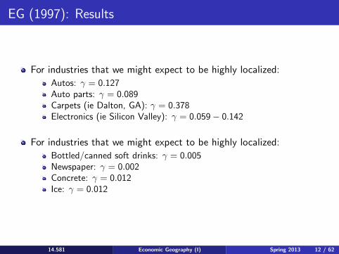
EG (1997): Results
For industries that we might expect to be highly localized: Autos: γ = 0.127 Auto parts: γ = 0.089 Carpets (ie Dalton, GA): γ = 0.378 Electronics (ie Silicon Valley): γ = 0.059 − 0.142
For industries that we might expect to be highly localized: Bottled/canned soft drinks: γ = 0.005 Newspaper: γ = 0.002 Concrete: γ = 0.012 Ice: γ = 0.012
14.581 Economic Geography (I) Spring 2013 12 / 62
EG (1997): Results
,PDJH�UHPRYHG�GXH�WR�FRS\ULJKW�UHVWULFWLRQV� � 6HH�)LJXUH���DQG�7DEOH���IURP��*HRJUDSKLF�&RQFHQWUDWLRQV�LQ�8�6� 0DQXIDFWXULQJ�,QGXVWLUHV��$�'DUWERDUG�$SSURDFK��
14.581 Economic Geography (I) Spring 2013 13 / 62

EG (1997): Results
Image removed due to copyright restrictions.
See Figure 1 and Table 4 from "Geographic Concentrations in
U.S. Manufacturing Industires: A Dartboard Approach."
14.581 Economic Geography (I) Spring 2013 14 / 62
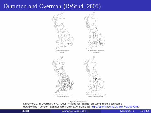
Duranton and Overman (ReStud, 2005)
(a) Basic Pharmaceuticals(SIC2441)
(b) Pharmaceutical Preparations(SIC2442)
(c) Other Agricultural and ForestryMachinery (SIC2932)
(d) Machinery for Textile, Apparel andLeather Production (SIC2954)
FIGURE 1
Maps of four illustrative industries
Duranton, G. & Overman, H.G. (2005. testing for localization using micro-geographic data [online]. London: LSE Research Online. Available at: http://eprints.lse.ac.uk/archive/00000581.
14.581 Economic Geography (I) Spring 2013 15 / 62

Plan for Two Lectures
1
2
Stylized facts about agglomeration of economic activity Testing sources of agglomeration:
1
2
3
Direct estimation Estimation from spatial equilibrium Estimation via tests for multiple equilibria
14.581 Economic Geography (I) Spring 2013 16 / 62
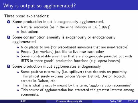
Why is output so agglomerated?
Three broad explanations: 1 Some production input is exogenously agglomerated.
Natural resources (as in the wine industry in EG (1997)) Institutions
2 Some consumption amenity is exogenously or endogenously agglomerated
Nice places to live (for place-based amenities that are non-tradable) People (i.e. workers) just like to live near each other Some non-tradable amenities that are endogenously provided but with IRTS in those goods’ production functions (e.g. opera houses)
3 Some production input agglomerates endogenously Some positive externality (i.e. spillover) that depends on proximity. This almost surely explains Silicon Valley, Detroit, Boston biotech, carpets in Dalton, etc. This is what is usually meant by the term, ‘agglomeration economies’ This source of agglomeration has attracted the greatest interest among economists.
14.581 Economic Geography (I) Spring 2013 17 / 62

What are sources of possible agglomeration economies?
The literature on this is enormous Probably begins in earnest with Marshall (1890) Recent survey in Duranton and Puga (2004, Handbook of Urban and Regional Econ)
Typically 3 forces for potential agglomeration economies: Thick input markets (reduce search costs and idiosyncratic risk) Increasing returns to scale combined with trade costs (on either inputs
1
2
3
or outputs) that scale with remoteness Knowledge spillovers
14.581 Economic Geography (I) Spring 2013 18 / 62

Empirical work on the causes of agglomeration
Recent surveys on this in: Redding (2010, J Reg. Sci. survey) Rosenthal and Strange (2004, Handbook of Urban and Regional Econ) Head and Mayer (2004, Handbook of Urban and Regional Econ) Overman, Redding and Venables (2004, Handbook of International Trade) Combes et al textbook, Economic Geography
Broadly, three approaches: Estimating agglomeration economies directly
Estimating agglomeration economies from the extent of agglomeration in an observed spatial equilibrium.
1
2
3 Testing for multiple equilibria (which is often a consequence of agglomeration economies)
14.581 Economic Geography (I) Spring 2013 19 / 62

Plan for Two Lectures
1
2
Stylized facts about agglomeration of economic activity Testing sources of agglomeration:
Direct estimation 1
2
3
Estimation from spatial equilibrium Estimation via tests for multiple equilibria
14.581 Economic Geography (I) Spring 2013 20 / 62
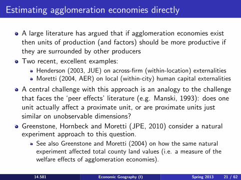
Estimating agglomeration economies directly
A large literature has argued that if agglomeration economies exist then units of production (and factors) should be more productive if they are surrounded by other producers Two recent, excellent examples:
Henderson (2003, JUE) on across-firm (within-location) externalities Moretti (2004, AER) on local (within-city) human capital externalities
A central challenge with this approach is an analogy to the challenge that faces the ‘peer effects’ literature (e.g. Manski, 1993): does one unit actually affect a proximate unit, or are proximate units just similar on unobservable dimensions? Greenstone, Hornbeck and Moretti (JPE, 2010) consider a natural experiment approach to this question.
See also Greenstone and Moretti (2004) on how the same natural experiment affected total county land values (i.e. a measure of the welfare effects of agglomeration economies).
14.581 Economic Geography (I) Spring 2013 21 / 62
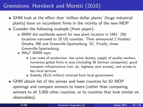
Greenstone, Hornbeck and Moretti (2010)
GHM look at the effect that ‘million dollar plants’ (huge industrial plants) have on incumbent firms in the vicinity of the new MDP Consider the following example (from paper):
BMW did worldwide search for new plant location in 1991. 250 locations narrowed to 20 US counties. Then announced 2 finalists: Omaha, NB and Greenville-Spartanburg, SC. Finally, chose Greenville-Spartanburg. Why? BMW says:
Low costs of production: low union density, supply of quality workers, numerous global firms in area (including 58 German companies), good transport infrastructure (rail, air, highway, port access), and access to key local services. Subsidy ($115 million) received from local government.
GHM obtain list of the winner and loser counties for 82 MDP openings and compare winners to losers (rather than comparing winners to all 3,000 other counties, or to counties that look similar on observables).
14.581 Economic Geography (I) Spring 2013 22 / 62
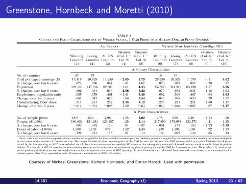
Greenstone, Hornbeck and Moretti (2010)
TABLE 3County and Plant Characteristics by Winner Status, 1 Year Prior to a Million Dollar Plant Opening
All Plants Within Same Industry (Two-Digit SIC)
WinningCounties
(1)
LosingCounties
(2)
All U.S.Counties
(3)
t-Statistic(Col. 1 �
Col. 2)(4)
t-Statistic(Col. 1 �
Col. 3)(5)
WinningCounties
(6)
LosingCounties
(7)
All U.S.Counties
(8)
t-Statistic(Col. 6 �
Col. 7)(9)
t-Statistic(Col. 6 �
Col. 8)(10)
A. County Characteristics
No. of counties 47 73 16 19Total per capita earnings ($) 17,418 20,628 11,259 �2.05 5.79 20,230 20,528 11,378 �.11 4.62% change, over last 6 years .074 .096 .037 �.81 1.67 .076 .089 .057 �.28 .57Population 322,745 447,876 82,381 �1.61 4.33 357,955 504,342 83,430 �1.17 3.26% change, over last 6 years .102 .051 .036 2.06 3.22 .070 .032 .031 1.18 1.63Employment-population ratio .535 .579 .461 �1.41 3.49 .602 .569 .467 .64 3.63Change, over last 6 years .041 .047 .023 �.68 2.54 .045 .038 .028 .39 1.57Manufacturing labor share .314 .251 .252 2.35 3.12 .296 .227 .251 1.60 1.17Change, over last 6 years �.014 �.031 �.008 1.52 �.64 �.030 �.040 �.007 .87 �3.17
B. Plant Characteristics
No. of sample plants 18.8 25.6 7.98 �1.35 3.02 2.75 3.92 2.38 �1.14 .70Output ($1,000s) 190,039 181,454 123,187 .25 2.14 217,950 178,958 132,571 .41 1.25% change, over last 6 years .082 .082 .118 .01 �.97 �.061 .177 .182 �1.23 �3.38Hours of labor (1,000s) 1,508 1,168 877 1.52 2.43 1,738 1,198 1,050 .92 1.33% change, over last 6 years .122 .081 .115 .81 .14 .160 .023 .144 .85 .13
Note.—For each case to be weighted equally, counties are weighted by the inverse of their number per case. Similarly, plants are weighted by the inverse of their number per county multipliedby the inverse of the number of counties per case. The sample includes all plants reporting data in the ASM for each year between the MDP opening and 8 years prior. Excluded are all plantsowned by the firm opening an MDP. Also excluded are all plants from two uncommon two-digit SIC values so that subsequently estimated clustered variance matrices would always be positivedefinite. The sample of all U.S. counties excludes winning counties and counties with no manufacturing plant reporting data in the ASM for 9 consecutive years. These other U.S. counties aregiven equal weight within years and are weighted across years to represent the years of MDP openings. Reported t-statistics are calculated from standard errors clustered at the county level. t-statistics greater than 2 are reported in bold. All monetary amounts are in 2006 U.S. dollars.
Courtesy of Michael Greenstone, Richard Hornbeck, and Enrico Moretti. Used with permission.
14.581 Economic Geography (I) Spring 2013 23 / 62
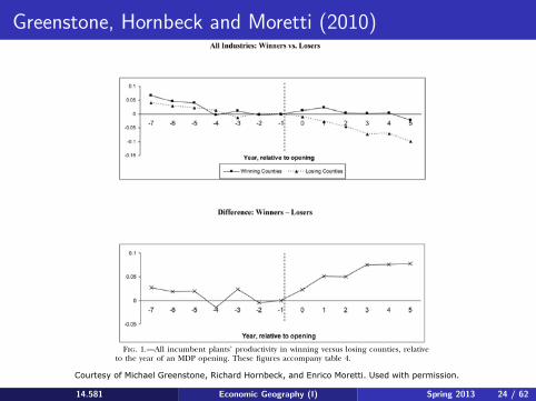
Fig. 1.—All incumbent plants’ productivity in winning versus losing counties, relativeto the year of an MDP opening. These figures accompany table 4.
Greenstone, Hornbeck and Moretti (2010)
Courtesy of Michael Greenstone, Richard Hornbeck, and Enrico Moretti. Used with permission.
14.581 Economic Geography (I) Spring 2013 24 / 62
Greenstone, Hornbeck and Moretti (2010)
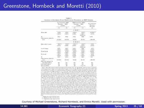
TABLE 5Changes in Incumbent Plant Productivity Following an MDP Opening
All Counties: MDPWinners � MDP
Losers
MDP Counties: MDPWinners � MDP
Losers
All Counties:RandomWinners
(5)(1) (2) (3) (4)
A. Model 1
Mean shift .0442* .0435* .0524** .0477** � 0.0496***(.0233) (.0235) (.0225) (.0231) (.0174)
[$170 m]2R .9811 .9812 .9812 .9860 ∼0.98
Observations (plant byyear) 418,064 418,064 50,842 28,732 ∼400,000
B. Model 2
Effect after 5 years .1301** .1324** .1355*** .1203** �.0296(.0533) (.0529) (.0477) (.0517) (.0434)
[$429 m]Level change .0277 .0251 .0255 .0290 .0073
(.0241) (.0221) (.0186) (.0210) (.0223)Trend break .0171* .0179** .0183** .0152* � 0.0062
(.0091) (.0088) (.0078) (.0079) (.0063)Pre-trend �.0057 �.0058 �.0048 �.0044 �.0048
(.0046) (.0046) (.0046) (.0044) (.0040)2R .9811 .9812 .9813 .9861 ∼.98
Observations (plant byyear) 418,064 418,064 50,842 28,732 ∼400,000
Plant and industry byyear fixed effects Yes Yes Yes Yes Yes
Case fixed effects No Yes Yes Yes NAYears included All All All �7 ≤ t ≤ 5 All
Note.—The table reports results from fitting several versions of eq. (8). Specifically, entries are from a regressionof the natural log of output on the natural log of inputs, year by two-digit SIC fixed effects, plant fixed effects, andcase fixed effects. In model 1, two additional dummy variables are included for whether the plant is in a winning county7 to 1 years before the MDP opening or 0 to 5 years after. The reported mean shift indicates the difference in thesetwo coefficients, i.e., the average change in TFP following the opening. In model 2, the same two dummy variables areincluded along with pre- and post-trend variables. The shift in level and trend are reported, along with the pre-trendand the total effect evaluated after 5 years. In cols. 1, 2, and 5, the sample is composed of all manufacturing plants inthe ASM that report data for 14 consecutive years, excluding all plants owned by the MDP firm. In these models,additional control variables are included for the event years outside the range from through (i.e., �20t p �7 t p 5to �8 and 6 to 17). Column 2 adds the case fixed effects that equal one during the period that t ranges from �7through 5. In cols. 3 and 4, the sample is restricted to include only plants in counties that won or lost an MDP. Thisforces the industry by year fixed effects to be estimated solely from plants in these counties. For col. 4, the sample isrestricted further to include only plant by year observations within the period of interest (where t ranges from �7 to5). This forces the industry by year fixed effects to be estimated solely on plant by year observations that identify theparameters of interest. In col. 5, a set of 47 plant openings in the entire country were randomly chosen from the ASMin the same years and industries as the MDP openings (this procedure was run 1,000 times, and reported are the meansand standard deviations of those estimates). For all regressions, plant by year observations are weighted by the plant’stotal value of shipments 8 years prior to the opening. Plants not in a winning or losing county are weighted by theirtotal value of shipments in that year. All plants from two uncommon two-digit SIC values were excluded so that estimatedclustered variance-covariance matrices would always be positive definite. In brackets is the value in 2006 U.S. dollarsfrom the estimated increase in productivity: the percentage increase is multiplied by the total value of output for theaffected incumbent plants in the winning counties. Reported in parentheses are standard errors clustered at the countylevel.
* Significant at the 10 percent level.** Significant at the 5 percent level.*** Significant at the 1 percent level.
14.581 Economic Geography (I) Spring 2013 25 / 62
Courtesy of Michael Greenstone, Richard Hornbeck, and Enrico Moretti. Used with permission.
Greenstone, Hornbeck and Moretti (2010)
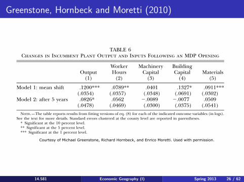
TABLE 6Changes in Incumbent Plant Output and Inputs Following an MDP Opening
Output(1)
WorkerHours
(2)
MachineryCapital
(3)
BuildingCapital
(4)Materials
(5)
Model 1: mean shift .1200*** .0789** .0401 .1327* .0911***(.0354) (.0357) (.0348) (.0691) (.0302)
Model 2: after 5 years .0826* .0562 �.0089 �.0077 .0509(.0478) (.0469) (.0300) (.0375) (.0541)
Note.—The table reports results from fitting versions of eq. (8) for each of the indicated outcome variables (in logs).See the text for more details. Standard errors clustered at the county level are reported in parentheses.
* Significant at the 10 percent level.** Significant at the 5 percent level.*** Significant at the 1 percent level.
opening.2614.581 Economic Geography (I) Spring 2013 26 / 62
Courtesy of Michael Greenstone, Richard Hornbeck, and Enrico Moretti. Used with permission.
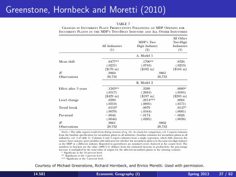
Greenstone, Hornbeck and Moretti (2010) TABLE 7
Changes in Incumbent Plant Productivity Following an MDP Opening forIncumbent Plants in the MDP’s Two-Digit Industry and All Other Industries
All Industries(1)
MDP’s Two-Digit Industry
(2)
All OtherTwo-DigitIndustries
(3)
A. Model 1
Mean shift .0477** .1700** .0326(.0231) (.0743) (.0253)
[$170 m] [$102 m] [$104 m]2R .9860 .9861
Observations 28,732 28,732
B. Model 2
Effect after 5 years .1203** .3289 .0889*(.0517) (.2684) (.0504)
[$429 m] [$197 m] [$283 m]Level change .0290 .2814*** .0004
(.0210) (.0895) (.0171)Trend break .0152* .0079 .0147*
(.0079) (.0344) (.0081)Pre-trend �.0044 �.0174 �.0026
(.0044) (.0265) (.0036)2R .9861 .9862
Observations 28,732 28,732
Note.—The table reports results from fitting versions of eq. (8). As a basis for comparison, col. 1 reports estimatesfrom the baseline specification for incumbent plants in all industries (baseline estimates for incumbent plants in allindustries, col. 4 of table 5). Columns 2 and 3 report estimates from a single regression, which fully interacts thewinner/loser and pre/post variables with indicators for whether the incumbent plant is in the same two-digit industryas the MDP or a different industry. Reported in parentheses are standard errors clustered at the county level. Thenumbers in brackets are the value (2006 U.S. dollars) from the estimated increase in productivity: the percentageincrease is multiplied by the total value of output for the affected incumbent plants in the winning counties.
* Significant at the 10 percent level.** Significant at the 5 percent level.*** Significant at the 1 percent level.
Courtesy of Michael Greenstone, Richard Hornbeck, and Enrico Moretti. Used with permission.
14.581 Economic Geography (I) Spring 2013 27 / 62

Greenstone, Hornbeck and Moretti (2010) TABLE 8
Changes in Incumbent Plant Productivity Following an MDP Opening, byMeasures of Economic Distance between the MDP’s Industry and Incumbent
Plant’s Industry
(1) (2) (3) (4) (5) (6) (7)
CPS workertransitions .0701*** .0374
(.0237) (.0260)Citation pattern .0545*** .0256
(.0192) (.0208)Technology
input .0320* .0501(.0173) (.0421)
Technologyoutput .0596*** .0004
(.0216) (.0434)Manufacturing
input .0060 �.0473(.0123) (.0289)
Manufacturingoutput .0150 �.0145
(.0196) (.0230)2R .9852 .9852 .9851 .9852 .9851 .9852 .9853
Observations 23,397 23,397 23,397 23,397 23,397 23,397 23,397
Note.—The table reports results from fitting versions of eq. (9), which is modified from eq. (8). Building on themodel 1 specification in col. 4 of table 5, each column adds interaction terms between winner/loser and pre/poststatus with the indicated measures of how an incumbent plant’s industry is linked to its associated MDP’s industry (acontinuous version of results in table 7). These industry linkage measures are defined and described in table 2, andhere the measures are normalized to have a mean of zero and a standard deviation of one. The sample of plants isthat in col. 4 of table 5, but it is restricted to plants that have industry linkage data for each measure. For assigningthis linkage measure, the incumbent plant’s industry is held fixed at its industry the year prior to the MDP opening.Whenever a plant is a winner or loser more than once, it receives an additive dummy variable and interaction termfor each occurrence. Reported in parentheses are standard errors clustered at the county level.
* Significant at the 10 percent level.** Significant at the 5 percent level.*** Significant at the 1 percent level.
Courtesy of Michael Greenstone, Richard Hornbeck, and Enrico Moretti. Used with permission.
14.581 Economic Geography (I) Spring 2013 28 / 62
Greenstone, Hornbeck and Moretti (2010)
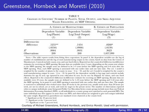
TABLE 9Changes in Counties’ Number of Plants, Total Output, and Skill-Adjusted
Wages Following an MDP Opening
A. Census of Manufactures B. Census of Population
Dependent Variable:Log(Plants)
(1)
Dependent Variable:Log(Total Output)
(2)
Dependent Variable:Log(Wage)
(3)
Difference-in-difference .1255** .1454 .0268*
(.0550) (.0900) (.0139)2R .9984 .9931 .3623
Observations 209 209 1,057,999
Note.—The table reports results from fitting three regressions. In panel A, the dependent variables are the log ofnumber of establishments and the log of total manufacturing output in the county, based on data from the Census ofManufactures. Controls include county, year, and case fixed effects. Reported are the county-level difference-in-differenceestimates for receiving an MDP opening. Because data are available every 5 years, depending on the census year relativeto the MDP opening, the sample years are defined to be 1–5 years before the MDP opening and 4–8 years after theMDP opening. Thus, each MDP opening is associated with one earlier date and one later date. The col. 1 model isweighted by the number of plants in the county in years �6 to �10, and the col. 2 model is weighted by the county’stotal manufacturing output in years �6 to �10. In panel B, the dependent variable is log wage and controls includedummies for age by year, age squared by year, education by year, sex by race by Hispanic by citizen, and case fixedeffects. Reported is the county-level difference-in-difference estimate for receiving an MDP opening. Because data areavailable every 10 years, the sample years are defined to be 1–10 years before the MDP opening and 3–12 years afterthe MDP opening. As in panel A, each MDP opening is associated with one earlier date and one later date. The sampleis restricted to individuals who worked more than 26 weeks in the previous year, usually work more than 20 hours perweek, are not in school, are at work, and work for wages in the private sector. The number of observations reportedrefers to unique individuals: some Integrated Public Use Microdata Series county groups include more than one FederalInformation Processing Standard (FIPS), so all individuals in a county group were matched to each potential FIPS. Thesame individual may then appear in more than one FIPS, and observations are weighted to give each unique individualthe same weight. Reported in parentheses are standard errors clustered at the county level.
* Significant at the 10 percent level.** Significant at the 5 percent level.*** Significant at the 1 percent level.
14.581 Economic Geography (I) Spring 2013 29 / 62
Courtesy of Michael Greenstone, Richard Hornbeck, and Enrico Moretti. Used with permission.

Plan for Two Lectures
1
2
Stylized facts about agglomeration of economic activity Testing sources of agglomeration:
1
2
3
Direct estimation Estimation from spatial equilibrium Estimation via tests for multiple equilibria
14.581 Economic Geography (I) Spring 2013 30 / 62

Market Access Approaches
A large literature has considered how the economic activity of a region depends on that of other, nearby regions.
A very common approach (to the challenge of parameterizing how one region affects another) is to work with the concept of ‘market access’. We will cover this approach now.
MA is usually defined in the context of a one-sector Krugman (1980) model but an observationally equivalent expression would derive in any one-sector gravity model (including neoclassical models without any externalities). So while the MA approach is interesting it doesn’t directly map to the estimation of agglomeration externalities.
However, we will also discuss recent approaches that add agglomeration externalities on top of a one-sector gravity model such that there is now a genuine agglomeration externality that can be estimated.
14.581 Economic Geography (I) Spring 2013 31 / 62

Redding and Venables (JIE, 2004): Set-up
Consider a (one-sector) gravity model with:
d Xd θXod = Ao c −θτ−θ
od Sd τ−θ od P = So (1)o
Where co is the cost of a unit input bundle in country o, τ is the trade cost and Pd is the consumer price index in d . So and Sd are origin and destination-specific fixed-effects, respectively.
β Pγ o where wo is the price of immobile αNow suppose that co = wo vo
factors, vo = v is the price of mobile factors and Po is the price index of a basket of intermediate inputs.
14.581 Economic Geography (I) Spring 2013 32 / 62
Redding and Venables (JIE, 2004): Set-up
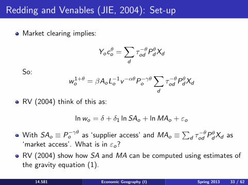
Market clearing implies: θ τ−θPθYo c =o od d Xd
d
So: 1+θ −αθP−γθ w = βAo L
−1 v τ−θPd θXdo o o od
d
RV (2004) think of this as:
ln wo = δ + δ1 ln SAo + ln MAo + εo With SAo ≡ Po
−γθ as ‘supplier access’ and MAo ≡ τ−θPθXd asd od d ‘market access’. What is in εo ?
RV (2004) show how SA and MA can be computed using estimates of the gravity equation (1).
14.581 Economic Geography (I) Spring 2013 33 / 62
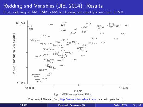
Redding and Venables (JIE, 2004): Results First, look only at MA. FMA is MA but leaving out country’s own term in MA.
Fig. 1. GDP per capita and FMA.
Courtesy of Elsevier, Inc., http://www.sciencedirect.com. Used with permission.
14.581 Economic Geography (I) Spring 2013 34 / 62
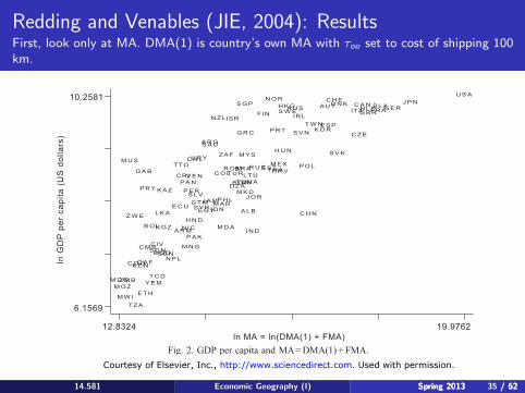
Redding and Venables (JIE, 2004): Results First, look only at MA. DMA(1) is country’s own MA with τoo set to cost of shipping 100 km.
Fig. 2. GDP per capita and MA=DMA(1) + FMA.
Courtesy of Elsevier, Inc., http://www.sciencedirect.com. Used with permission.
14.581 Economic Geography (I) Spring 2013 35 / 62Spring 2013 / 62
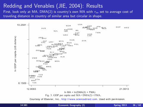
Redding and Venables (JIE, 2004): Results First, look only at MA. DMA(2) is country’s own MA with τoo set to average cost of traveling distance in country of similar area but circular in shape.
Fig. 3. GDP per capita and MA=DMA(2) + FMA.
&RXUWHV\�RI�(OVHYLHU��,QF���KWWS���ZZZ�VFLHQFHGLUHFW�FRP��8VHG�ZLWK�SHUPLVVLRQ�
14.581 Economic Geography (I) Spring 2013 36 / 62

Redding and Venables (JIE, 2004): Results First, look only at MA. DMA(3) is country’s own MA with τoo set as in DMA(2) but with half the distance elasticity as for τod .
Fig. 4. GDP per capita and MA=DMA(3) + FMA.��(OVHYLHU��,QF��$OO�ULJKWV�UHVHUYHG��7KLV�FRQWHQW�LV�H[FOXGHG�IURP�RXU�&UHDWLYH &RPPRQV�OLFHQVH��)RU�PRUH�LQIRUPDWLRQ��VHH�KWWS���RFZ�PLW�HGX�IDLUXVH�
14.581 Economic Geography (I) Spring 2013 37 / 62
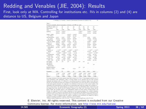
Redding and Venables (JIE, 2004): Results First, look only at MA. Controlling for institutions etc. IVs in columns (2) and (4) are distance to US, Belgium and Japan
Table 3
Economic geography, physical geography, institutions, and GDP per capita
ln(GDP per capita) (1) (2) (3) (4) (5) (6) (7) (8)
Observations 91 91 91 91 101 101 69 69
Year 1996 1996 1996 1996 1996 1996 1996 1996
ln(FMAi) 0.215**
[0.063]
0.229**
[0.083]
– 0.148**
[0.061]
– 0.269**
[0.112]
0.189**
[0.096]
ln(MAi =DMAi
(3) + FMAi)
– – 0.307**
[0.066]
0.256**
[0.124]
0.337**
[0.063]
ln(hydrocarbons
per capita)
0.019
[0.015]
0.019
[0.015]
0.018
[0.021]
0.019
[0.024]
– – 0.026
[0.018]
0.026
[0.018]
ln(arable land
area per capita)
� 0.050
[0.066]
� 0.050
[0.070]
0.161
[0.103]
0.126
[0.136]
– – � 0.078
[0.085]
� 0.107
[0.088]
Number of
minerals
0.016**
[0.008]
0.016
[0.010]
� 0.017
[0.013]
� 0.013
[0.015]
– – 0.015
[0.014]
0.012
[0.014]
Fraction land in
geographical
tropics
� 0.057
[0.239]
� 0.041
[0.257]
0.128
[0.293]
0.056
[0.347]
– – 0.175
[0.294]
0.077
[0.286]
Prevalence of
malaria
� 1.107**
[0.282]
� 1.097**
[0.284]
� 1.008**
[0.376]
� 1.052**
[0.403]
– – � 1.105**
[0.318]
� 1.163**
[0.325]
Risk of
expropriation
� 0.445**
[0.091]
� 0.441**
[0.093]
� 0.181
[0.129]
� 0.236
[0.172]
– – � 0.361**
[0.116]
� 0.376**
[0.116]
Socialist rule
1950–1995
� 0.210
[0.191]
� 0.218
[0.192]
� 0.050
[0.208]
� 0.056
[0.214]
– – � 0.099
[0.241]
� 0.069
[0.248]
External war
1960–1985
� 0.052
[0.169]
� 0.051
[0.174]
0.001
[0.312]
� 0.012
[0.307]
– – � 0.078
[0.209]
� 0.093
[0.210]
Full sample yes yes yes yes yes yes
Non-OECD yes
Non-OECD+
OECD FMA
yes
Regional dummies yes yes
Sargan ( p-value) – 0.980 – 0.721 – – – –
Estimation OLS IV OLS IV OLS OLS OLS OLS
R2 0.766 0.766 0.842 0.839 0.688 0.837 0.669 0.654
F(�) 47.77 53.00 59.07 64.76 58.00 67.53 18.23 17.80
Prob>F 0.000 0.000 0.000 0.000 0.000 0.000 0.000 0.000
First-stage estimation of the trade equation using Tobit (column (3) in Table 1). Bootstrapped standard errors in
square parentheses (200 replications). FMAi is Foreign Market Access obtained from the trade equation
estimation and defined in Eq. (17); DMAi(3) is our preferred measure of Domestic Market Access that uses
internal area information but allows the coefficient on internal distance to be lower than that on external distance
in the trade equation estimation. See Appendix A for definitions of and sources for the control variables. The
availability of the hydrocarbons per capita and risk of expropriation data reduces the sample size in columns (1)–
(4) to 91 observations. The regional dummies in columns (5) and (6) are Sub-Saharan Africa, North Africa and
the Middle East, Latin America and the Caribbean, Southeast Asia, Other Asia, and Eastern Europe and the
former USSR. The excluded category is the industrialized countries of North America, Western Europe, and
Oceania. See Appendix A for the country composition of each regional grouping. The excluded exogenous
variables in columns (2) and (4) are log distance from the US, log distance from Belgium (as a central point in the
European Union), and log distance from Japan. Sargan is a Sargan test of the model’s overidentifying restrictions.
In column (7), FMA is computed using all countries, estimation on the non-OECD. In column (8), FMA is
computed excluding non-OECD countries, estimation on the non-OECD.
*Denotes statistical significance at the 10% level. **Denotes statistical significance at the 5% level.
S. Redding, A.J. Venables / Journal of International Economics 62 (2004) 53–82 69
��(OVHYLHU��,QF��$OO�ULJKWV�UHVHUYHG��7KLV�FRQWHQW�LV�H[FOXGHG�IURP�RXU�&UHDWLYH &RPPRQV�OLFHQVH��)RU�PRUH�LQIRUPDWLRQ��VHH�KWWS���RFZ�PLW�HGX�IDLUXVH�
14.581 Economic Geography (I) Spring 2013 38 / 62
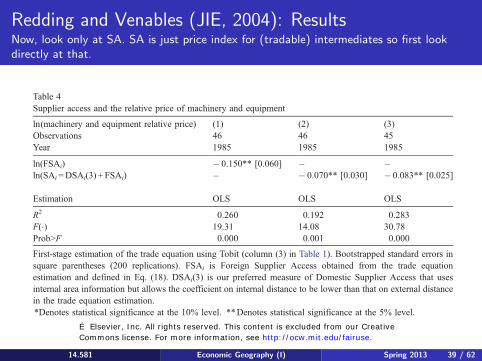
Redding and Venables (JIE, 2004): Results Now, look only at SA. SA is just price index for (tradable) intermediates so first look directly at that.
Table 4
Supplier access and the relative price of machinery and equipment
ln(machinery and equipment relative price) (1) (2) (3)
Observations 46 46 45
Year 1985 1985 1985
ln(FSAi) � 0.150** [0.060] – –
ln(SAi =DSAi(3) + FSAi) – � 0.070** [0.030] � 0.083** [0.025]
Estimation OLS OLS OLS
R2 0.260 0.192 0.283
F(�) 19.31 14.08 30.78
Prob>F 0.000 0.001 0.000
First-stage estimation of the trade equation using Tobit (column (3) in Table 1). Bootstrapped standard errors in
square parentheses (200 replications). FSAi is Foreign Supplier Access obtained from the trade equation
estimation and defined in Eq. (18). DSAi(3) is our preferred measure of Domestic Supplier Access that uses
internal area information but allows the coefficient on internal distance to be lower than that on external distance
in the trade equation estimation.
*Denotes statistical significance at the 10% level. **Denotes statistical significance at the 5% level.
��(OVHYLHU��,QF��$OO�ULJKWV�UHVHUYHG��7KLV�FRQWHQW�LV�H[FOXGHG�IURP�RXU�&UHDWLYH &RPPRQV�OLFHQVH��)RU�PRUH�LQIRUPDWLRQ��VHH�KWWS���RFZ�PLW�HGX�IDLUXVH�
14.581 Economic Geography (I) Spring 2013 39 / 62
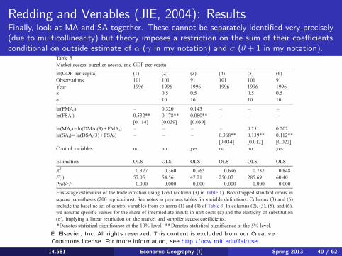
Table 5
Market access, supplier access, and GDP per capita
ln(GDP per capita) (1) (2) (3) (4) (5) (6)
Observations 101 101 91 101 101 91
Year 1996 1996 1996 1996 1996 1996
a 0.5 0.5 0.5 0.5
r 10 10 10 10
ln(FMAi) – 0.320 0.143 – – –
ln(FSAi) 0.532**
[0.114]
0.178**
[0.039]
0.080**
[0.039]
– – –
ln(MAi) = ln(DMAi(3) + FMAi) – – – – 0.251 0.202
ln(SAi) = ln(DSAi(3) + FSAi) – – – 0.368**
[0.034]
0.139**
[0.012]
0.112**
[0.022]
Control variables no no yes no no yes
Estimation OLS OLS OLS OLS OLS OLS
R2 0.377 0.360 0.765 0.696 0.732 0.848
F(�) 57.05 54.56 47.21 250.07 285.69 60.40
Prob>F 0.000 0.000 0.000 0.000 0.000 0.000
First-stage estimation of the trade equation using Tobit (column (3) in Table 1). Bootstrapped standard errors in
square parentheses (200 replications). See notes to previous tables for variable definitions. Columns (3) and (6)
include the baseline set of control variables from columns (1) and (4) of Table 3. In columns (2), (3), (5), and (6),
we assume specific values for the share of intermediate inputs in unit costs (a) and the elasticity of substitution
(r), implying a linear restriction on the market and supplier access coefficients.
*Denotes statistical significance at the 10% level. **Denotes statistical significance at the 5% level.
Redding and Venables (JIE, 2004): Results Finally, look at MA and SA together. These cannot be separately identified very precisely (due to multicollinearity) but theory imposes a restriction on the sum of their coefficients conditional on outside estimate of α (γ in my notation) and σ (θ + 1 in my notation).
��(OVHYLHU��,QF��$OO�ULJKWV�UHVHUYHG��7KLV�FRQWHQW�LV�H[FOXGHG�IURP�RXU�&UHDWLYH &RPPRQV�OLFHQVH��)RU�PRUH�LQIRUPDWLRQ��VHH�KWWS���RFZ�PLW�HGX�IDLUXVH�
14.581 Economic Geography (I) Spring 2013 40 / 62
Redding and Sturm (AER, 2008)
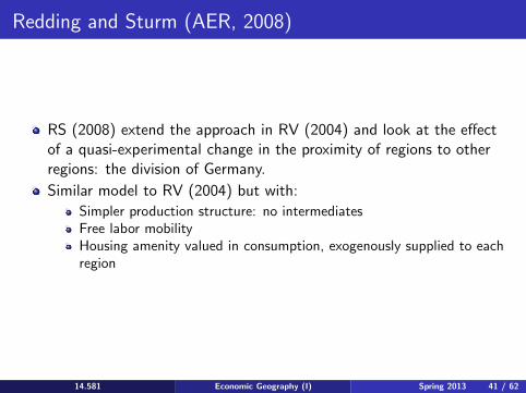
RS (2008) extend the approach in RV (2004) and look at the effect of a quasi-experimental change in the proximity of regions to other regions: the division of Germany. Similar model to RV (2004) but with:
Simpler production structure: no intermediates Free labor mobility Housing amenity valued in consumption, exogenously supplied to each region
14.581 Economic Geography (I) Spring 2013 41 / 62
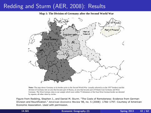
Map 1: The Division of Germany after the Second World War
Notes: The map shows Germany in its borders prior to the Second World War (usually referred to as the 1937 borders) and the division of Germany into an area that became part of Russia, an area that became part of Poland, East Germany and West Germany. The West German cities in our sample which were within 75 kilometers of the East-West German border are denoted by squares, all other cities by circles.
Redding and Sturm (AER, 2008): Results
Figure from Redding, Stephen J., and Daniel M. Sturm. "The Costs of Remoteness: Evidence from German Division and Reunification." American Economic Review 98, no. 5 (2008): 1766–1797. Courtesy of American Economic Association. Used with permission.
14.581 Economic Geography (I) Spring 2013 42 / 62
Figures 3 and 4
11.
21.
41.
61.
8
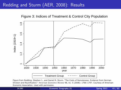
1920 1930 1940 1950 1960 1970 1980 1990 2000year
Treatment Group Control Group
Inde
x (1
919=
1)Figure 3: Indices of Treatment & Control City Population
−0.
3−
0.2
−0.
10.
0
1920 1930 1940 1950 1960 1970 1980 1990 2000year
Tre
atm
ent G
roup
− C
ontr
ol G
roup
Figure 4: Difference in Population Indices, Treatment − Control
Redding and Sturm (AER, 2008): Results
Figure from Redding, Stephen J., and Daniel M. Sturm. "The Costs of Remoteness: Evidence from German Division and Reunification." American Economic Review 98, no. 5 (2008): 1766–1797. Courtesy of American Economic Association. Used with permission.
14.581 Economic Geography (I) Spring 2013 43 / 62
Redding and Sturm (AER, 2008): Results
−4
−2
02
4D
ivis
ion
Tre
atm
ent
0 100 200 300Distance to East−West German Border (km)
Simulated Treatment Estimated Treatment
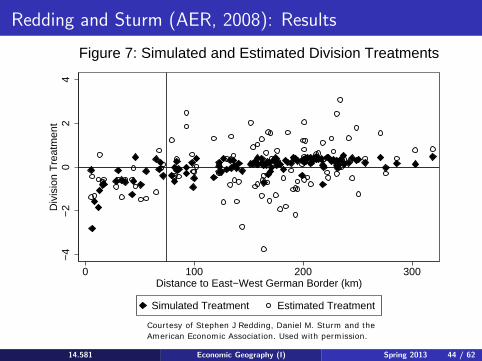
Figure 7: Simulated and Estimated Division Treatments
14.581 Economic Geography (I) Spring 2013 44 / 62
&RXUWHV\�RI�6WHSKHQ�-�5HGGLQJ��'DQLHO�0��6WXUP�DQG�WKH $PHULFDQ�(FRQRPLF�$VVRFLDWLRQ��8VHG�ZLWK�SHUPLVVLRQ�
Donaldson and Hornbeck (2013)
DH (2013) also pursue a MA approach, in the context of studying the impact of railroads on the US economy (1870-1890)
MA is not the focus here. Instead, the goal is to develop a regression approach for the study of railroad access on local prosperity (as measured through land values) that is robust to econometric spillovers. MA delivers this.
14.581 Economic Geography (I) Spring 2013 45 / 62
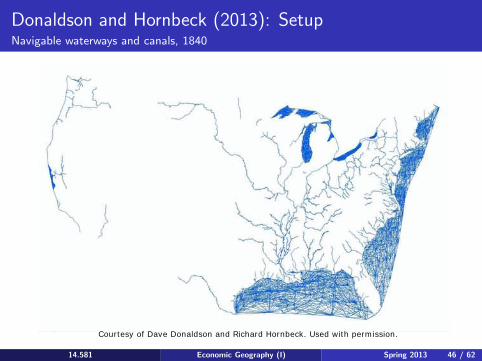
Donaldson and Hornbeck (2013): Setup Navigable waterways and canals, 1840
&RXUWHV\�RI�'DYH�'RQDOGVRQ�DQG�5LFKDUG�+RUQEHFN��8VHG�ZLWK�SHUPLVVLRQ�
14.581 Economic Geography (I) Spring 2013 46 / 62
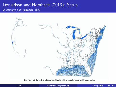
Donaldson and Hornbeck (2013): Setup Waterways and railroads, 1850
Courtesy of Dave Donaldson and Richard Hornbeck. Used with permission.
14.581 Economic Geography (I) Spring 2013 47 / 62
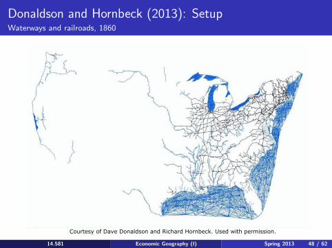
Donaldson and Hornbeck (2013): Setup Waterways and railroads, 1860
Courtesy of Dave Donaldson and Richard Hornbeck. Used with permission.
14.581 Economic Geography (I) Spring 2013 48 / 62
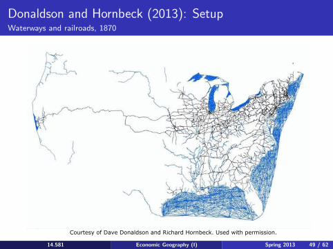
Donaldson and Hornbeck (2013): Setup Waterways and railroads, 1870
Courtesy of Dave Donaldson and Richard Hornbeck. Used with permission.
14.581 Economic Geography (I) Spring 2013 49 / 62
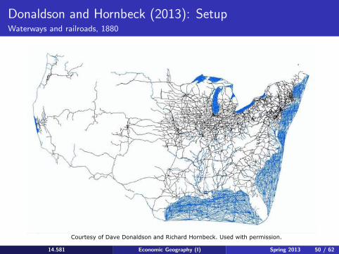
Donaldson and Hornbeck (2013): Setup Waterways and railroads, 1880
Courtesy of Dave Donaldson and Richard Hornbeck. Used with permission.
14.581 Economic Geography (I) Spring 2013 50 / 62

Donaldson and Hornbeck (2013): Setup Waterways and railroads, 1887
Courtesy of Dave Donaldson and Richard Hornbeck. Used with permission.
14.581 Economic Geography (I) Spring 2013 51 / 62
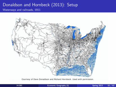
Donaldson and Hornbeck (2013): Setup Waterways and railroads, 1911
14.581 Economic Geography (I) Spring 2013 52 / 62
&RXUWHV\�RI�'DYH�'RQDOGVRQ�DQG�5LFKDUG�+RUQEHFN��8VHG�ZLWK�SHUPLVVLRQ�
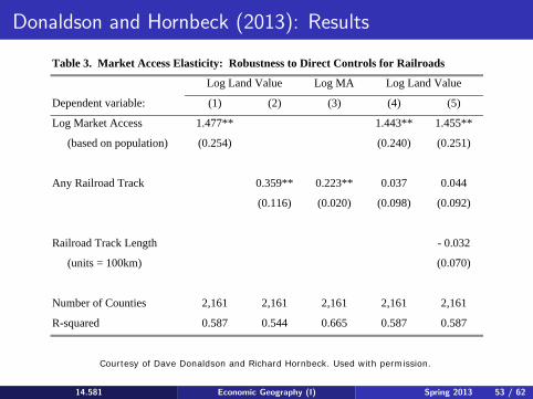
Table 3. Market Access Elasticity: Robustness to Direct Controls for Railroads
Log MA
(1) (2) (3) (4) (5)
Log Market Access 1.477** 1.443** 1.455**
(based on population) (0.254) (0.240) (0.251)
Any Railroad Track 0.359** 0.223** 0.037 0.044
(0.116) (0.020) (0.098) (0.092)
Railroad Track Length - 0.032
(units = 100km) (0.070)
Number of Counties 2,161 2,161 2,161 2,161 2,161
R-squared 0.587 0.544 0.665 0.587 0.587
Dependent variable:
Log Land ValueLog Land Value
Donaldson and Hornbeck (2013): Results
&RXUWHV\�RI�'DYH�'RQDOGVRQ�DQG�5LFKDUG�+RUQEHFN��8VHG�ZLWK�SHUPLVVLRQ�
14.581 Economic Geography (I) Spring 2013 53 / 62
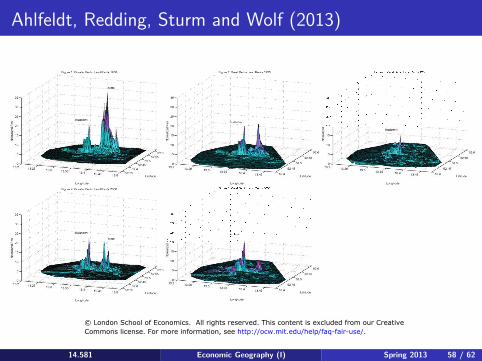
Ahlfeldt, Redding, Sturm and Wolf (2013)
ARSW (2013) develop a similar approach to RS (2008) but to the case of the division (and reunification) of Berlin. So this is about the importance of proximity at a very different spatial scale (neighborhoods rather than regions).
Paper looks at the effect of the loss of access/proximity to the downtown region (CBD/“Mitte”), which was in East Berlin, on neighborhoods of West Berlin. And then the reverse for reunification.
14.581 Economic Geography (I) Spring 2013 54 / 62
Ahlfeldt, Redding, Sturm and Wolf (2013)
Model is similar to RS (2008) but with some alterations: Commuting costs that vary with distance. This is modeled in the standard ‘logit’ fashion where workers’ places of residence are fixed but they then receive exogenous utility shocks for each location and they choose the utility maximizing work location (as a function of the utility shocks, the wage, and the commuting cost). No trade costs (the logic here is that most of what was produced in Berlin was exported to the rest of the ‘world’ anyway. Consumer amenities that depend on an exogenous local term (as in RS, 2008) and a distance-weighted sum of all other regions’ populations. Production externalities that depend on an exogenous local term and a distance-weighted sum of all other regions’ employment .
14.581 Economic Geography (I) Spring 2013 55 / 62
Ahlfeldt, Redding, Sturm and Wolf (2013)
Basic estimation strategy: Basic principle is that this is a model with a parameter for agglomeration externalities. ARSW then let the data, when fed through the model, identify that parameter. Analogous to approach summarized in Glaeser and Gottlieb (JEL, 2010)—more detail in Glaeser’s 2009 book of lectures on urban economics—or Allen and Arkolakis (2013). Formulate moments based on the identifying assumption that the (unobserved) production/consumption amenities (for each location) don’t change over time in a way that is correlated with distance to the CBD. This effectively says that the only effect of distance-to-the-CBD is working through the model’s 3 distance-dependent terms (production externalities, consumption externalities, and commuting costs). Remarkably, there is sufficient variation in these 3 terms to allow identification of 3 separate parameters.
14.581 Economic Geography (I) Spring 2013 56 / 62
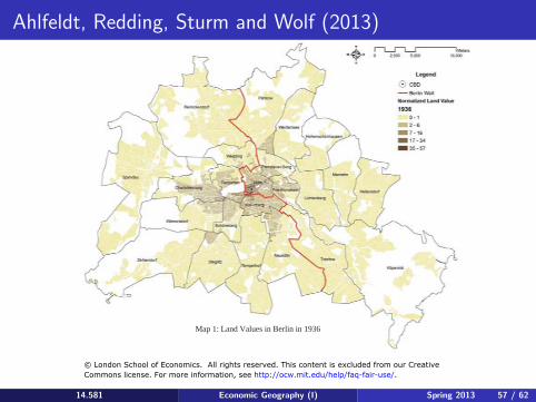
Map 1: Land Values in Berlin in 1936
Ahlfeldt, Redding, Sturm and Wolf (2013)
14.581 Economic Geography (I) Spring 2013 57 / 62
© London School of Economics. All rights reserved. This content is excluded from our CreativeCommons license. For more information, see http://ocw.mit.edu/help/faq-fair-use/.
Ahlfeldt, Redding, Sturm and Wolf (2013)
14.581 Economic Geography (I) Spring 2013 58 / 62
© London School of Economics. All rights reserved. This content is excluded from our CreativeCommons license. For more information, see http://ocw.mit.edu/help/faq-fair-use/.
-4-2
02
Log
Diff
eren
ce in
Nor
mal
ized
Ren
t
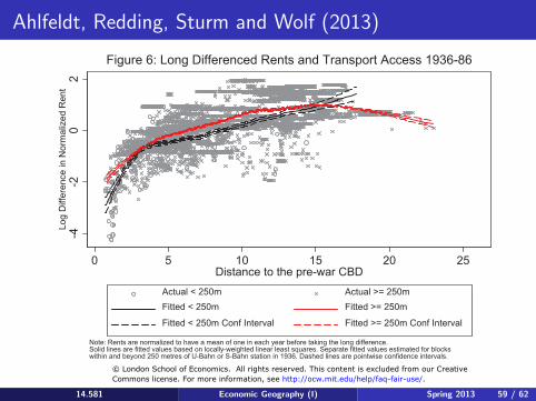
0 5 10 15 20 25Distance to the pre-war CBD
Actual < 250m Actual >= 250mFitted < 250m Fitted >= 250m
Fitted < 250m Conf Interval Fitted >= 250m Conf Interval
Note: Rents are normalized to have a mean of one in each year before taking the long difference.Solid lines are fitted values based on locally-weighted linear least squares. Separate fitted values estimated for blocks within and beyond 250 metres of U-Bahn or S-Bahn station in 1936. Dashed lines are pointwise confidence intervals.
Figure 6: Long Differenced Rents and Transport Access 1936-86
Ahlfeldt, Redding, Sturm and Wolf (2013)
14.581 Economic Geography (I) Spring 2013 59 / 62
© London School of Economics. All rights reserved. This content is excluded from our CreativeCommons license. For more information, see http://ocw.mit.edu/help/faq-fair-use/.

Ahlfeldt, Redding, Sturm and Wolf (2013)
-10
12
3Lo
g D
iffer
ence
in N
orm
aliz
ed R
ent
0 5 10 15 20 25Distance to the pre-war CBD
Actual < 250m Actual >= 250mFitted < 250m Fitted >= 250m
Fitted < 250m Conf Interval Fitted >= 250m Conf Interval
Note: Rents are normalized to have a mean of one in each year before taking the long difference.Solid lines are fitted values based on locally-weighted linear least squares. Separate fitted values estimated for blocks within and beyond 250 metres of U-Bahn or S-Bahn station in 1936. Dashed lines are pointwise confidence intervals.
Figure 7: Long Differenced Rents and Transport Access 1986-2006
14.581 Economic Geography (I) Spring 2013 60 / 62
© London School of Economics. All rights reserved. This content is excluded from our CreativeCommons license. For more information, see http://ocw.mit.edu/help/faq-fair-use/.
Ahlfeldt, Redding, Sturm and Wolf (2013)
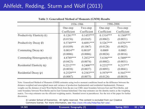
One-step Two-step One-step Two-stepCoefficient Coefficient Coefficient Coefficient
Productivity Elasticity (�) 0.1261*** 0.1455*** 0.1314*** 0.1369***(0.0156) (0.0165) (0.0062) (0.0031)
Productivity Decay (�) 0.5749*** 0.6091*** 0.5267*** 0.8791***(0.0189) (0.1067) (0.0128) (0.0025)
Commuting Decay (�) 0.0014** 0.0010* 0.0009 0.0005(0.0006) (0.0006) (0.0024) (0.0016)
Commuting Heterogeneity (�) 4.8789*** 5.2832*** 5.6186*** 6.5409***(0.0423) (0.0074) (0.0082) (0.0031)
Residential Elasticity (�) 0.2212*** 0.2400*** 0.2232*** 0.215***(0.0038) (0.0037) (0.0093) (0.0041)
Residential Decay (�) 0.2529*** 0.2583*** 0.5979*** 0.5647***(0.0087) (0.0075) (0.0124) (0.0019)
Note: Generalized Method of Moments (GMM) estimates using twelve moment conditions based on the difference between the distance-weighted and unweighted mean and variance of production fundamentals and residential fundamentals. Distance weights use the distance of each West Berlin block from the pre-war CBD, inner boundary between East and West Berlin, and outer boundary between West Berlin and its East German hinterland. One-step estimates use the identity matrix as the weighting matrix. Two-step estimates use the efficient weighting matrix. Standard errors in parentheses. See the text of the paper for further discussion.
1936-1986 1986-2006
Table 3: Generalized Method of Moments (GMM) Results
14.581 Economic Geography (I) Spring 2013 61 / 62
© London School of Economics. All rights reserved. This content is excluded from our CreativeCommons license. For more information, see http://ocw.mit.edu/help/faq-fair-use/.
Ahlfeldt, Redding, Sturm and Wolf (2013)
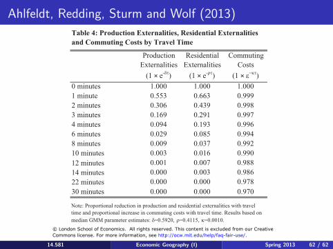
ProductionExternalities
(1 × e-��)
ResidentialExternalities
(1 × e-��)
CommutingCosts
(1 × ���0 minutes 1.000 1.000 1.0001 minute 0.553 0.663 0.9992 minutes 0.306 0.439 0.9983 minutes 0.169 0.291 0.9974 minutes 0.094 0.193 0.9966 minutes 0.029 0.085 0.9948 minutes 0.009 0.037 0.99210 minutes 0.003 0.016 0.99012 minutes 0.001 0.007 0.98814 minutes 0.000 0.003 0.98622 minutes 0.000 0.000 0.97830 minutes 0.000 0.000 0.970
Table 4: Production Externalities, Residential Externalities and Commuting Costs by Travel Time
Note: Proportional reduction in production and residential externalities with travel time and proportional increase in commuting costs with travel time. Results based on median GMM parameter estimates: �=0.5920, �=0.4115, �=0.0010.
14.581 Economic Geography (I) Spring 2013 62 / 62
© London School of Economics. All rights reserved. This content is excluded from our CreativeCommons license. For more information, see http://ocw.mit.edu/help/faq-fair-use/.

MIT OpenCourseWarehttp://ocw.mit.edu
14.581 International Economics ISpring 2013
For information about citing these materials or our Terms of Use, visit: http://ocw.mit.edu/terms.