Embed Size (px)
Citation preview

—
14.581
Spring 2013
14.581 Economic Geography (II) Spring 2013 1 / 25
14.581 International Trade— Lecture 21: Economic Geography (II)—
14.581
Spring 2013

Plan for Two Lectures
1
2
Stylized facts about agglomeration of economic activity Testing sources of agglomeration:
1 Direct estimation 2 Estimation from spatial equilibrium 3 Estimation via tests for multiple equilibria
14.581 Economic Geography (II) Spring 2013 2 / 25

Plan for Two Lectures
1 Stylized facts about agglomeration of economic activity Testing sources of agglomeration: 2
1
2
Direct estimation Estimation from spatial equilibrium
3 Estimation via tests for multiple equilibria
14.581 Economic Geography (II) Spring 2013 3 / 25

Krugman (JPE, 1991): Basic Setup
This is an extremely influential paper on a theory of economic geography (8,500 cites).
It formalizes, in an extremely simple and clear manner, one particular form of agglomeration externality: that which arises with the combination of IRTS in production and trade costs.
At a more prosaic level, this is just Krugman (1980) with the added assumption of free labor mobility.
14.581 Economic Geography (II) Spring 2013 4 / 25

Krugman (JPE, 1991): Aside on HME Empirics
Core of Krugman (1980) and the reason for agglomeration in Krugman (1991) is the ‘home market effect’.
We should therefore ask what independent evidence there is for the HME (regardless of agglomeration externalities). This is also of interest in its own right as the HME has been highlighted as the one testable empirical prediction that differs strongly across neoclassical and IRTS-based models of trade. On this, see:
Davis and Weinstein (JIE, 2003) Hanson and Xiang (AER, 2004) Behrens et al (2009) Head and Ries (2001) Feenstra, Markusen and Rose (2004)
But the punchline is that there is no one convincing test. The reason is that it is (of course) challenging to come up with a plausible source of exogenous demand shocks (which lie at the heart of the HME).
14.581 Economic Geography (II) Spring 2013 5 / 25

Krugman (JPE, 1991): Basic Setup
2 regions 2 sectors:
‘Agriculture’: CRTS, freely traded, workers immobile geographically ‘Manufacturing’: IRTS (Dixit-Stiglitz with CES preferences), iceberg trade costs τ , mobile workers Cobb-Douglas preferences between A and M sectors
Basic logic can have other interpretations: Krugman and Venables (QJE, 1995): immobile factors but input-output linkages between two Dixit-Stiglitz sectors Baldwin (1999): endogenous factor accumulation rather than factor mobility And others; see Robert-Nicoud (2005) or a synthesis and simplification to the ‘core’ of these models.
Hard to extend beyond 2 regions, but see: Krugman and Venables (1995, wp) for a continuous space version (on a circle) Fujita, Krugman and Venables (1999 book) for a wealthy discussion of extensions to the basic logic (and more)
14.581 Economic Geography (II) Spring 2013 6 / 25

Krugman (1991): Key Result sH is the share of mobile workers in one location (call it H) relative to the other location; φ ≡ τ 1−σ is index of freeness of trade
Figure 1: The Tomahawk Diagram
1/2
φ
sH
0
1
1φBφS
called ‘tomahawk’ diagram, Figure 1 (the ‘tomahawk’ moniker come14.581 Economic Geography (II) Spring 2013 7 / 25

Davis and Weinstein (AER, 2002)
DW (2002) ask whether regions/cities’ population levels respond to one-off shocks
The application is to WWII bombing in Japan Their findings are surprising and have been replicated in many other settings:
Germany (WWII): Brakman, Garretsen and Schramm (2004) Vietnam (Vietnam war): Miguel and Roland (2011) ...
Davis and Weinstein (J Reg. Sci., 2008) extend the analysis in DW (2002) to the case of the fate of industry-locations. This is doubly interesting as it is plausible that industrial activity is mobile across space in ways that people are not.

Davis and Weinstein (2002)
Davis, Donald R., and David E. Weinstein. "Bones, Bombs, and Break Points: The Geography
of Economic Activity." American Economic Review 92 no. 5 (2002): 1269–89.,
Courtesy of American Economic Association. Used with permission.
14.581 Economic Geography (II) Spring 2013 / 259

Davis and Weinstein (2002)
14.581 Economic Geography (II) Spring 2013 10 / 25
Davis, Donald R., and David E. Weinstein. "Bones, Bombs, and Break Points: The Geography
of Economic Activity." American Economic Review 92, no. 5 (2002): 1269–89.
Courtesy of American Economic Association. Used with permission.

Davis and Weinstein (2008)
Table 2
Correlation of Growth Rates of Industries Within Cities 1938 to 1948
Machinery Metals Chemicals Textiles Food Printing LumberMetals 0.60Chemicals 0.30 0.36Textiles 0.12 0.35 0.25Food 0.32 0.65 0.31 0.49Printing 0.11 0.30 0.04 0.29 0.35Lumber 0.23 0.35 0.21 0.25 0.25 0.41Ceramics 0.13 0.53 0.36 0.38 0.50 0.41 0.23
14.581 Economic Geography (II) Spring 2013 11 / 25
Metals
Chemicals
Textiles and Apparel
Lumber and Wood
Stone, Clay, Glass
252.9
187.0
270.2
124.6
79.4
36.9
91.6
20.5
29.4
13.5
-85%
-51%
Manufacturing 206.2 27.4 -87%
Machinery 639.2 38.0 -94%
-92%
Processed Food 89.9 54.2 -40%
Printing and Publishing 133.5 32.7 -76%
-76%
-83%
Industry 1941 Change1946
Evolution of Japanese manufacturing during World War II (Quantum Indices from Japanese Economic Statistics)
Image by MIT OpenCourseWare.

Davis and Weinstein (2008)
Table 1 Evolution of Japanese manufacturing during World War II (Quantum Indices from Japanese Economic Statistics)
14.581 Economic Geography (II) Spring 2013 12 / 25
Machinery
Metals
Chemicals
Food
Lumber
Printing
Ceramics
0.60 0.30 0.12 0.32 0.11 0.23 0.13
0.250.29
-
0.31
0.49
-
0.25
-
-
-
0.36
-
-
0.35
-- -
0.65
- -
0.35
0.04
0.30 0.35
0.21
0.25
0.41
- 0.23
0.41
0.50
0.38
0.36
0.53
-
-
-
-
-
-
-
-
Chemicals Food LumberMetals PrintingTextiles
Textiles
Correlation of Growth Rates of Industries Within Cities 1938 to 1948
Image by MIT OpenCourseWare.

Davis and Weinstein (2008)
14.581 Economic Geography (II) Spring 2013 13 / 25
Bridges 3.5
7.0
10.8
14.8
16.8
21.9
24.6
34.3
80.6
Railroads and tramways
Electric power generation facilities
Telecommunication facilities
Water and sewerage works
Cars
Buildings
Industrial machinery and equipment
Ships
Harbors and canals 7.5
Total 25.4
Decline
Inflation Adjusted Percent Decline in Assets Between 1935 and 1945
Image by MIT OpenCourseWare.

Davis and Weinstein (2008)
Nor
mal
ized
Gro
wth
(19
48 t
o 19
69)
Normalized Growth (1938 to 1948)
-5 0 5
-5
0
5
FIGURE 7: Mean-Differenced Industry Growth Rates.
14.581 Economic Geography
(I
I) Spring
2013 14 / 25
Davis, Donald R., and David E. Weinstein. "Bones, Bombs, and Break Points: The Geography of Economic Activity." American Economic Review 92, no. 5 (2002): 1269–1289. Courtesy of American Economic Association. Used with permission.
Davis and Weinstein (2008)
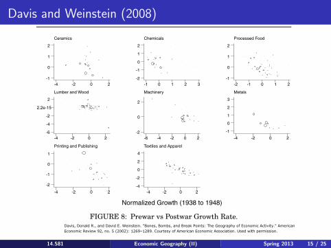
Normalized Growth (1938 to 1948)
Ceramics
-4 -2 0 2-1
0
1
2
Chemicals
-1 0 1 2 3-2
-1
0
1
2
Processed Food
-2 -1 0 1 2-1
0
1
2
Lumber and Wood
-4 -2 0 2-6
-4
-2
2.2e-15
2
Machinery
-6 -4 -2 0 2-2
0
2
Metals
-4 -2 0 2
-1
0
1
2
3
Printing and Publishing
-4 -2 0 2
-2
-1
0
1
Textiles and Apparel
-4 -2 0 2-4
-2
0
2
4
FIGURE 8: Prewar vs Postwar Growth Rate.
that the coefficient on the wartime (1940–1947) growth rate is minus unity. Wecannot reject a coefficient of minus unity, hence cannot reject a null that there isa unique stable equilibrium. We also find that regionally-directed governmentreconstruction expenses following the war had no significant impact on citysizes 20 years after the war.
We next apply our threshold regression approach described above to testingfor multiple equilibria. This places unique and multiple equilibria on an evenfooting. The results are reported in the remaining columns of Table 4. In column2 of Table 4, we present the results for the estimation of equation (11) in the casein which there is a unique equilibrium. Given how close our previous estimateof � was to 0 (minus unity on wartime growth), it is not surprising that theestimates of the other parameters do not change much when we constrain � totake on this value.
Columns 3–5 present the results for threshold regressions premised onvarious numbers of equilibria.15 In these regressions, the constant plus �1 is
15In principle, we could have considered the possibility of more than four equilibria. However,neither the data plots nor any of the regression results suggested that raising the number ofpotential equilibria was likely to improve the results.
C© Blackwell Publishing, Inc. 2008.
14.581 Economic Geography (II) Spring 2013 15 / 25
Davis, Donald R., and David E. Weinstein. "Bones, Bombs, and Break Points: The Geography of Economic Activity." AmericanEconomic Review 92, no. 5 (2002): 1269–1289. Courtesy of American Economic Association. Used with permission.

Bleakley and Lin (QJE, 2012)
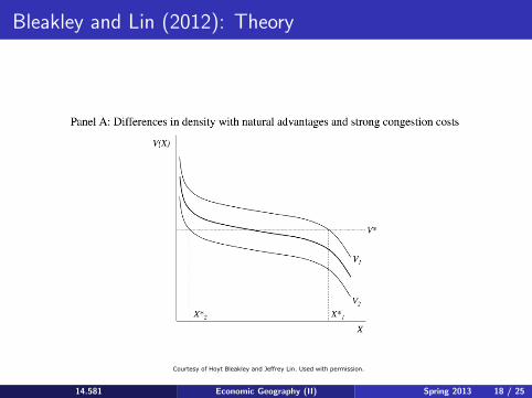
BL (2012) look for an even that removed a location’s natural (i.e. exogenous) productivity advantage/amenity.
If there are no agglomeration externalities then this location will suffer from this removal.
But if there are agglomeration externalities then this location might not suffer much at all. Its future success is assured through the logic of multiple equilibria. (This is typically referred to as ‘path dependence’.)
14.581 Economic Geography (II) Spring 2013 16 / 25

Bleakley and Lin (QJE, 2012): Portage
What is the natural advantage that got removed from some locations?
BL (2012) look at ‘portage sites’: locations where portage (i.e. the trans-shipment of goods from one type of boat to another type of boat) took place before the construction of canals/railroads. Prior to canals/railroads portage was extremely labor-intensive so portage sites were a source of excess labor demand.
What is an exogenous source for a portage site? BL (2012) use the ‘fall line’, a geological feature indicating the point at which (in the US) navigable rivers leaving the ocean would first become unnavigable
14.581 Economic Geography (II) Spring 2013 17 / 25
14.581 Economic Geography (II) Spring 2013 18 / 25
Courtesy of Hoyt Bleakley and Jeffrey Lin. Used with permission.
Bleakley and Lin (2012): Theory

14.581 Economic Geography (II) Spring 2013 19 / 25
Courtesy of Hoyt Bleakley and Jeffrey Lin. Used with permission.
Bleakley and Lin (2012): Theory

FIGURE A.1The Density Near Fall-Line/River Intersections
This map shows the contemporary distribution of economic activity across the southeastern United States measured by the 2003nighttime lights layer. For information on sources, see notes for Figures II and IV.
at MIT Libraries on April 30, 2013 http://qje.oxfordjournals.org/ Downloaded from
14.581 Economic Geography (II) Spring 2013 20 / 25
Courtesy of Jeffrey Lin and Hoyt Bleakley. Used with permission.
Bleakley and Lin (2010): The Fall Line

PORTAGE AND PATH DEPENDENCE 601
FIGURE IIFall-Line Cities from Alabama to North Carolina
The map in the upper panel shows the contemporary distribution of economicactivity across the southeastern United States, measured by the 2003 nighttimelights layer from NationalAtlas.gov. The nighttime lights are used to present anearly continuous measure of present-day economic activity at a high spatialfrequency. The fall line (solid) is digitized from Physical Divisions of the UnitedStates, produced by the U.S. Geological Survey. Major rivers (dashed gray) arefrom NationalAtlas.gov, based on data produced by the United States GeologicalSurvey. Contemporary fall-line cities are labeled in the lower panel.
We can see the importance of fall-line/river intersections bylooking along the paths of rivers. Along a given river, there is
14.581 Economic Geography (II) Spring 2013 21 / 25
Courtesy of Hoyt Bleakley and Jeffrey Lin. Used with permission.
Bleakley and Lin (2012): The Fall Line

Bleakley and Lin (2012): The Fall Line
14.581 Economic Geography (II) Spring 2013 22 / 25
FIGURE IVFall-Line Cities from North Carolina to New Jersey
The map in the left panel shows the contemporary distribution of economicactivity across the southeastern United States measured by the 2003 nighttimelights layer from NationalAtlas.gov. The nighttime lights are used to presenta nearly continuous measure of present-day economic activity at a high spatialfrequency. The fall line (solid) is digitized from Physical Divisions of the UnitedStates, produced by the U.S. Geological Survey. Major rivers (dashed gray) arefrom NationalAtlas.gov, based on data produced by the U.S. Geological Survey.Contemporary fall-line cities are labeled in the right panel.
Courtesy of Hoyt Bleakley and Jeffrey Lin. Used with permission.

FIGURE IIIPopulation Density in 2000 along Fall-Line Rivers
These graphs display contemporary population density along fall-line rivers.We select census 2000 tracts whose centroids lie within 50 miles along fall-linerivers; the horizontal axis measures distance to the fall line, where the fall lineis normalized to zero, and the Atlantic Ocean lies to the left. In Panel A, thesedistances are calculated in miles. In Panel B, these distances are normalized foreach river relative tothe river mouth or the river source. The rawpopulation dataare then smoothed via Stata’s lowess procedure, with bandwidths of 0.3 (Panel A)or 0.1 (Panel B).
fall line. This comparison is useful in the following sense: today,all of the sites along the river have the advantage of being alongthe river, but only at the fall line was there an initial portage
14.581 Economic Geography (II) Spring 2013 23 / 25
Courtesy of Jeffrey Lin and Hoyt Bleakley. Used with permission.
Courtesy of Hoyt Bleakley and Jeffrey Lin. Used with permission.
Bleakley and Lin (2012): Results

TABLE II
UPSTREAM WATERSHED AND CONTEMPORARY POPULATION DENSITY
(1) (2) (3) (4) (5)Basic Other spatial controls Water power
Specifications:State fixed
effects
Distancefrom various
features
Explanatory variables:Panel A: Census Tracts, 2000, N = 21452Portage site times
upstream watershed0.467 0.467 0.500 0.496 0.452
(0.175)∗∗ (0.164)∗∗∗ (0.114)∗∗∗ (0.173)∗∗∗ (0.177)∗∗
Binary indicatorfor portage site
1.096 1.000 1.111 1.099 1.056(0.348)∗∗∗ (0.326)∗∗∗ (0.219)∗∗∗ (0.350)∗∗∗ (0.364)∗∗∗
Portage site timeshorsepower/100k
−1.812(1.235)
Portage site timesI(horsepower> 2000)
0.110(0.311)
Panel B: Nighttime Lights, 1996–97, N = 65000Portage site times
upstream watershed0.418 0.352 0.456 0.415 0.393
(0.115)∗∗∗ (0.102)∗∗∗ (0.113)∗∗∗ (0.116)∗∗∗ (0.111)∗∗∗
Binary indicatorfor portage site
0.463 0.424 0.421 0.462 0.368(0.116)∗∗∗ (0.111)∗∗∗ (0.121)∗∗∗ (0.116)∗∗∗ (0.132)∗∗∗
Portage site timeshorsepower/100k
0.098(0.433)
Portage site timesI(horsepower> 2000)
0.318(0.232)
Panel C: Counties, 2000, N = 3480Portage site times
upstream watershed0.443 0.372 0.423 0.462 0.328
(0.209)∗∗ (0.185)∗∗ (0.207)∗∗ (0.215)∗∗ (0.154)∗∗
Binary indicator forportage site
0.890 0.834 0.742 0.889 0.587(0.211)∗∗∗ (0.194)∗∗∗ (0.232)∗∗∗ (0.211)∗∗∗ (0.210)∗∗∗
Portage site timeshorsepower/100k
−0.460(0.771)
Portage site timesI(horsepower> 2000)
0.991(0.442)
14.581 Economic Geography (II) Spring 2013 24 / 25
Courtesy of Hoyt Bleakley and Jeffrey Lin. Used with permission.
Bleakley and Lin (2012): Results

Bleakley and Lin (2012): Results
TABLE III
PROXIMITY TO HISTORICAL PORTAGE SITE AND HISTORICAL FACTORS
(1) (2) (3) (4) (5) (6) (7) (8) (9) (10)
Baseline
Railroadnetworklength,1850
Distanceto RR
hub, 1850
Literatewhite
men, 1850
Literacyrate whitemen, 1850
Collegeteachers
per capita,1850
Manuf. /agric.,1880
Non-agr.share,1880
Industrialdiversity(1-digit),
1880
Industrialdiversity(3-digit),
1880
Water powerin use 1885,
dummy
Explanatory variables:Panel A. Portage and historical factorsDummy for proximity
to portage site1.451 −0.656 0.557 0.013 0.240 0.065 0.073 0.143 0.927 0.164
(0.304)∗∗∗ (0.254)∗∗ (0.222)∗∗ (0.014) (0.179) (0.024)∗∗∗ (0.025)∗∗∗ (0.078)∗ (0.339)∗∗∗ (0.053)∗∗∗
Panel B. Portage and historical factors, conditioned on historical densityDummy for proximity
to portage site1.023 −0.451 0.021 −0.003 0.213 0.022 0.019 0.033 −0.091 0.169
(0.297)∗∗∗ (0.270) (0.035) (0.014) (0.162) (0.019) (0.019) (0.074) (0.262) (0.054)∗∗∗
Panel C. Portage and contemporary density, conditioned on historical factorsDummy for proximity
to portage site0.912 0.774 0.751 0.729 0.940 0.883 0.833 0.784 0.847 0.691 0.872
(0.236)∗∗∗ (0.236)∗∗∗ (0.258)∗∗∗ (0.187)∗∗∗ (0.237)∗∗∗ (0.229)∗∗∗ (0.227)∗∗∗ (0.222)∗∗∗ (0.251)∗∗∗ (0.221)∗∗∗ (0.233)∗∗∗
Historical factor 0.118 −0.098 0.439 0.666 1.349 1.989 2.390 0.838 0.310 0.331(0.024)∗∗∗ (0.022)∗∗∗ (0.069)∗∗∗ (0.389)∗ (0.164)∗∗∗ (0.165)∗∗∗ (0.315)∗∗∗ (0.055)∗∗∗ (0.015)∗∗∗ (0.152)∗∗
Notes. This table displays estimates of equation 1, with the below noted modifications. In Panels A and B, the outcome variables are historical factor densities, as noted in thecolumn headings. The main explanatory variable is a dummy for proximity to a historical portage. Panel B also controls for historical population density. In Panel C, the outcomevariable is 2000 population density, measured in natural logarithms, and the explanatory variables are portage proximity and the historical factor density noted in the columnheading. Each panel/column presents estimates from a separate regression. The sample consists of all U.S. counties, in each historical year, that are within the watersheds of riversthat cross the fall line. The estimator used is OLS, with standard errors clustered on the 53 watersheds. The basic specification includes a polynomial in latitude and longitude, a setof fixed effects by the watershed of each river that crosses the fall line, and dummies for proximity to the fall line and to a river. Reporting of additional coefficients is suppressed.Data sources and additional variable and sample definitions are found in the text and appendixes.
14.581 Economic Geography (II) Spring 2013 25 / 25
Courtesy of Hoyt Bleakley and Jeffrey Lin. Used with permission.
Bleakley and Lin (2012): Results

MIT OpenCourseWarehttp://ocw.mit.edu
14.581 International Economics ISpring 2013
For information about citing these materials or our Terms of Use, visit: http://ocw.mit.edu/terms.