1.6 Delay and Loss in Packet-Switched Networks

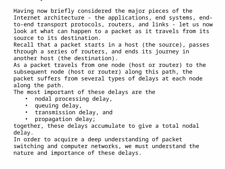
Having now briefly considered the major pieces of the Internet architecture - the applications, end systems, end-to-end transport protocols, routers, and links - let us now look at what can happen to a packet as it travels from its source to its destination. Recall that a packet starts in a host (the source), passes through a series of routers, and ends its journey in another host (the destination). As a packet travels from one node (host or router) to the subsequent node (host or router) along this path, the packet suffers from several types of delays at each node along the path. The most important of these delays are the

• nodal processing delay, • queuing delay, • transmission delay, and • propagation delay;

together, these delays accumulate to give a total nodal delay. In order to acquire a deep understanding of packet switching and computer networks, we must understand the nature and importance of these delays.

1.6.1 Types of Delay

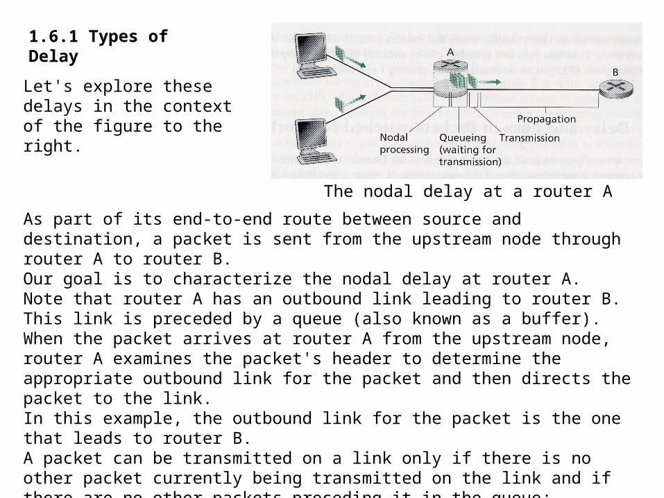
As part of its end-to-end route between source and destination, a packet is sent from the upstream node through router A to router B. Our goal is to characterize the nodal delay at router A. Note that router A has an outbound link leading to router B. This link is preceded by a queue (also known as a buffer). When the packet arrives at router A from the upstream node, router A examines the packet's header to determine the appropriate outbound link for the packet and then directs the packet to the link. In this example, the outbound link for the packet is the one that leads to router B. A packet can be transmitted on a link only if there is no other packet currently being transmitted on the link and if there are no other packets preceding it in the queue;if the link is currently busy or if there are other packets already queued for the link, the newly arriving packet will then join the queue.

The nodal delay at a router A

Let's explore these delays in the context of the figure to the right.

Processing Delay (dproc)The time required to examine the packet's header and determine where to direct the packet is part of the processing delay. The processing delay can also include other factors, such as the time needed to check for bit-level errors in the packet that occurred in transmitting the packet's bits from the upstream node to router A. Processing delays in high-speed routers are typically on the order of microseconds or less. After this nodal processing, the router directs the packet to the queue that precedes the link to router B. (In Chapter 4 we'll study the details of how a router operates.)

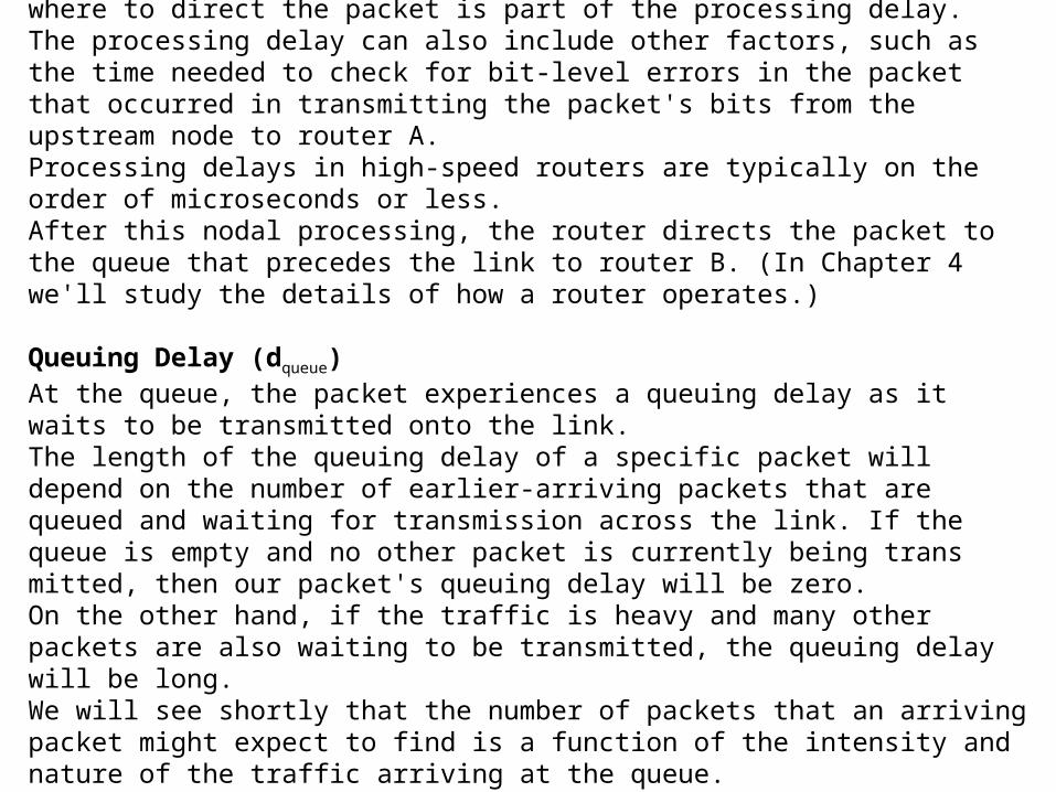
Queuing Delay (dqueue)At the queue, the packet experiences a queuing delay as it waits to be transmitted onto the link. The length of the queuing delay of a specific packet will depend on the number of earlier-arriving packets that are queued and waiting for transmission across the link. If the queue is empty and no other packet is currently being trans mitted, then our packet's queuing delay will be zero. On the other hand, if the traffic is heavy and many other packets are also waiting to be transmitted, the queuing delay will be long. We will see shortly that the number of packets that an arriving packet might expect to find is a function of the intensity and nature of the traffic arriving at the queue. Queuing delays can be on the order of microseconds to milliseconds in practice.

Transmission Delay (dtrans)Assuming that packets are transmitted in a first-come-first-served manner, as is common in packet-switched networks, our packet can be transmitted only after all the packets that have arrived before it have been transmitted. Denote the length of the packet by L bits, and denote the transmission rate of the link from router A to router B by R bits/sec. The rate R is determined by the transmission rate of the link to router B. For example, for a 10 Mbps Ethernet link, the rate is R = 10 Mbps; for a 100 Mbps Ethernet link, the rate is R = 100 Mbps. The transmission delay (also called the store-and-forward delay, as discussed in Section 1.3) is UR. This is the amount of time required to push (that is, transmit) all of the packet's bits into the link. Transmission delays are typically on the order of microseconds to milliseconds in practice.

Propagation Delay (dprop) Once a bit is pushed onto the link, it needs to propagate to router B. The time required to propagate from the beginning of the link to router B is the propagation delay. The bit propagates at the propagation speed of the link. The propagation speed depends on the physical medium of the link (that is, fiber optics, twisted-pair copper wire, and so on) and is in the range of   

2 • 108 meters/sec to 3 • 108 meters/sec which is equal to, or a little less than, the speed of light. The propagation delay is the distance between two routers divided by the propagation speed. That is, the propagation delay is d/s, where d is the distance between router A and router B and s is the propagation speed of the link. Once the last bit of the packet propagates to node B, it and all the preceding bits of the packet are stored in router B. The whole process then continues with router B now performing the forwarding.In wide-area networks, propagation delays are on the order of milliseconds.

Comparing Transmission and Propagation Delay

Newcomers to the field of computer networking sometimes have difficulty understanding the difference between transmission delay and propagation delay.

The difference is subtle but important.

The transmission delay is the amount of time required for the router to push out the packet; it is a function of the packet's length and the transmission rate of the link, but has nothing to do with the distance between the two routers.

The propagation delay, on the other hand, is the time it takes a bit to propagate from one router to the next; it is a function of the distance between the two routers, but has nothing to do with the packet's length or the transmission rate of the link.

An analogy might clarify the notions of transmission and propagation delay.Consider a highway that has a tollbooth every 100 kilometers. You can think of the highway segments between tollbooths as links and the tollbooths as routers. Suppose that cars travel (that is, propagate) on the highway at a rate of 100 km/hour (that is, when a car leaves a tollbooth, it instantaneously accelerates to 100 km/hour and maintains that speed between tollbooths). Suppose next that 10 cars, traveling together as a caravan follow each other in a fixed order. You can think of each car as a bit and the caravan as a packet. Also suppose that each tollbooth services (that is, transmits) a car at a rate of one car per 12 seconds, and that it is late at night so that the caravan's cars are the only cars on the highway. Finally, suppose that when ever the first car of the caravan arrives at a tollbooth, it waits at the entrance until the other nine cars have arrived and lined up behind it. (Thus the entire caravan must be stored at the tollbooth before it can begin to be forwarded.) The time required for the tollbooth to push the entire caravan onto the highway is (10 cars)/(5 cars/minute)= 2 minutes. This time is analogous to the transmission delay in a router. The time required for a car to travel from the exit of one tollbooth to the next tollbooth is 100 km/(100 km/hour) = 1 hour. This time is analogous to propagation delay. Therefore, the time from when the caravan is stored in front of a tollbooth until the caravan is stored in front of the next tollbooth is the sum of transmission delay and propagation delay—in this example, 62 minutes.

Let's explore this analogy a bit more. What would happen if the tollbooth service time for a caravan were greater than the time for a car to travel between toll-booths? For example, suppose now that the cars travel at the rate of 1,000 km/hour and the tollbooth services cars at the rate of one car per minute. Then the traveling delay between two tollbooths is 6 minutes and the time to serve a caravan is 10 minutes. In this case, the first few cars in the caravan will arrive at the second tollbooth before the last cars in the caravan leave the first tollbooth. This situation also arises in packet-switched networks - the first bits in a packet can arrive at a router while many of the remaining bits in the packet are still waiting to be transmitted by the preceding router.

If we let dproc denote the processing delay, dqueue denote the queuing delay, dtrans

denote the transmission delay, and dprop denote the propagation delay, then the total nodal delay dnodal is given by

 dnodal = dproc+ dqueue+ dtrans + dprop

 

The contribution of these delay components can vary significantly.

For example, dprop can be negligible (for example, a couple of microseconds) for a link connecting two routers on the same university campus; however, dprop is hundreds of milliseconds for two routers interconnected by a geostationary satellite link, and can be the dominant term in dnodal .

Similarly, dtrans can range from negligible to significant. Its contribution is typically negligible for transmission rates of 10 Mbps and higher (for example, for LANs); however, it can be hundreds of milliseconds for large Internet packets sent over low-speed dial-up modem links.

The processing delay, dproc, is often negligible; however, it strongly influences a router's maximum throughput, which is the maximum rate at which a router can forward packets.

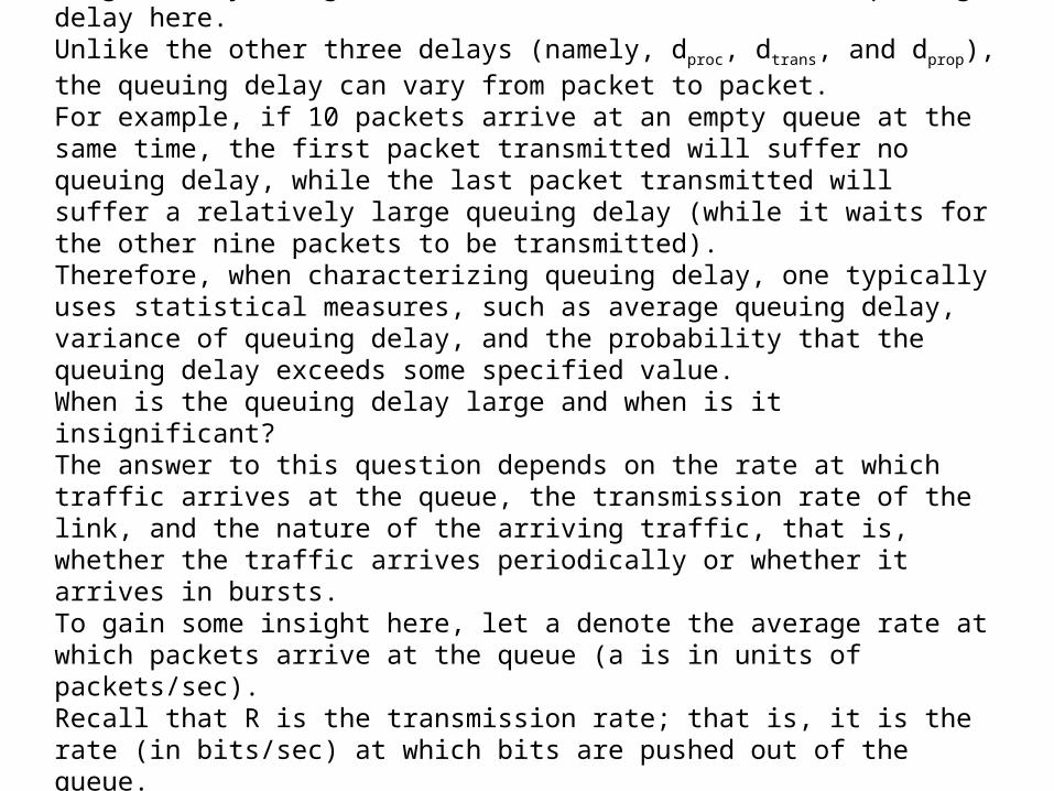
1.6.2 Queuing Delay and Packet LossThe most complicated and interesting component of nodal delay is the queuing delay, dqueue We give only a high-level, intuitive discussion of queuing delay here.Unlike the other three delays (namely, dproc, dtrans, and dprop), the queuing delay can vary from packet to packet. For example, if 10 packets arrive at an empty queue at the same time, the first packet transmitted will suffer no queuing delay, while the last packet transmitted will suffer a relatively large queuing delay (while it waits for the other nine packets to be transmitted). Therefore, when characterizing queuing delay, one typically uses statistical measures, such as average queuing delay, variance of queuing delay, and the probability that the queuing delay exceeds some specified value.When is the queuing delay large and when is it insignificant? The answer to this question depends on the rate at which traffic arrives at the queue, the transmission rate of the link, and the nature of the arriving traffic, that is, whether the traffic arrives periodically or whether it arrives in bursts. To gain some insight here, let a denote the average rate at which packets arrive at the queue (a is in units of packets/sec). Recall that R is the transmission rate; that is, it is the rate (in bits/sec) at which bits are pushed out of the queue. Also suppose, for simplicity, that all packets consist of L bits. Then the average rate at which bits arrive at the queue is La bits/sec.

Finally, assume that the queue is very big, so that it can hold essentially an infinite number of bits. The ratio La/R, called the traffic intensity, often plays an important role in estimating the extent of the queuing delay. If La/R > 1, then the average rate at which bits arrive at the queue exceeds the rate at which the bits can be transmitted from the queue. In this unfortunate situation, the queue will tend to increase without bound and the queuing delay will approach infinity! Therefore, one of the golden rules in traffic engineering is: Design your system so that the traffic intensity is no greater than 1. Now consider the case La/R < 1. Here, the nature of the arriving traffic impacts the queuing delay. For example, if packets arrive periodically—that is, one packet arrives every L/R seconds—then every packet will arrive at an empty queue and there will be no queuing delay. On the other hand, if packets arrive in bursts but periodically, there can be a significant average queuing delay. For example, suppose TV packets arrive simultaneously every (L/R)N seconds.Then the first packet transmitted has no queuing delay; the second packet transmitted has a queuing delay of L/R seconds; and more generally, the nth packet transmitted has a queuing delay of (n - 1)L/R seconds. We leave it as an exercise for you to calculate the average queuing delay in this example.

The two examples described above of periodic arrivals are a bit academic.Typically, the arrival process to a queue is random; that is, the arrivals do not follow any pattern and the packets are spaced apart by random amounts of time. In this more realistic case, the quantity La/R is not usually sufficient to fully characterize the delay statistics. Nonetheless, it is useful in gaining an intuitive understanding of the extent of the queuing delay. In particular, if traffic intensity is close to zero, then packet arrivals are few and far between and it is unlikely that an arriving packet will find another packet in the queue. Hence, the average queuing delay will be close to zero. On the other hand, when the traffic intensity is close to 1, there will be intervals of time when the arrival rate exceeds the transmission capacity (due to the burstiness of arrivals), and a queue will form. As the traffic intensity approaches 1, the average queue length gets larger and larger.

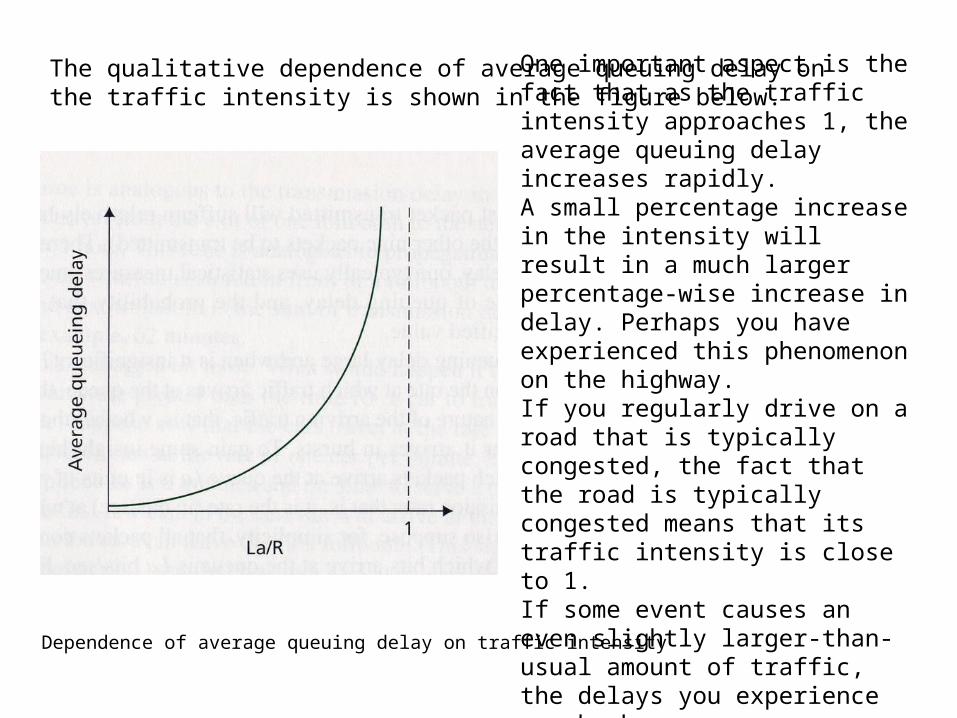
The qualitative dependence of average queuing delay on the traffic intensity is shown in the figure below.

Dependence of average queuing delay on traffic intensity

One important aspect is the fact that as the traffic intensity approaches 1, the average queuing delay increases rapidly. A small percentage increase in the intensity will result in a much larger percentage-wise increase in delay. Perhaps you have experienced this phenomenon on the highway. If you regularly drive on a road that is typically congested, the fact that the road is typically congested means that its traffic intensity is close to 1. If some event causes an even slightly larger-than-usual amount of traffic, the delays you experience can be huge.

Packet LossIn our discussions above, we have assumed that the queue is capable of holding an infinite number of packets. In reality a queue preceding a link has finite capacity, although the queuing capacity greatly depends on the switch design and cost. Because the queue capacity is finite, packet delays do not really approach infinity as the traffic intensity approaches 1. Instead, a packet can arrive to find a full queue. With no place to store such a packet, a router will drop that packet; that is, the packet will be lost. From an end-system viewpoint, this will look like a packet having been transmitted into the network core but never emerging from the network at the destination. The fraction of lost packets increases as the traffic intensity increases.Therefore, performance at a node is often measured not only in terms of delay, but also in terms of the probability of packet loss. As we'll discuss in the subsequent chapters, a lost packet may be retransmitted on an end-to-end basis, either by the application or by the transport layer protocol.

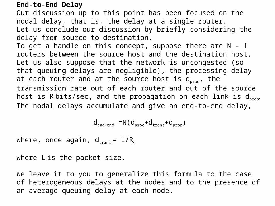
End-to-End DelayOur discussion up to this point has been focused on the nodal delay, that is, the delay at a single router. Let us conclude our discussion by briefly considering the delay from source to destination. To get a handle on this concept, suppose there are N - 1 routers between the source host and the destination host. Let us also suppose that the network is uncongested (so that queuing delays are negligible), the processing delay at each router and at the source host is dproc, the transmission rate out of each router and out of the source host is R bits/sec, and the propagation on each link is dprop. The nodal delays accumulate and give an end-to-end delay,

dend-end =N(dproc+dtrans+dprop)

where, once again, dtrans = L/R,

where L is the packet size.

We leave it to you to generalize this formula to the case of heterogeneous delays at the nodes and to the presence of an average queuing delay at each node.

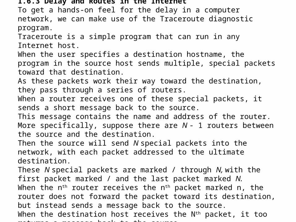
1.6.3 Delay and Routes in the InternetTo get a hands-on feel for the delay in a computer network, we can make use of the Traceroute diagnostic program. Traceroute is a simple program that can run in any Internet host. When the user specifies a destination hostname, the program in the source host sends multiple, special packets toward that destination. As these packets work their way toward the destination, they pass through a series of routers. When a router receives one of these special packets, it sends a short message back to the source. This message contains the name and address of the router.More specifically, suppose there are N - 1 routers between the source and the destination. Then the source will send N special packets into the network, with each packet addressed to the ultimate destination. These N special packets are marked / through N, with the first packet marked / and the last packet marked N. When the nth router receives the nth packet marked n, the router does not forward the packet toward its destination, but instead sends a message back to the source. When the destination host receives the Nth packet, it too returns a message back to the source.

The source records the time that elapses between when it sends a packet and when it receives the corresponding return message; it also records the name and address of the router (or the destination host) that returns the message. In this manner, the source can reconstruct the route taken by packets flowing from source to destination, and the source can determine the round-trip delays to all the intervening routers. Traceroute actually repeats the experiment just described three times, so the source actually sends 3 • N packets to the destination. RFC 1393 describes Traceroute in detail.

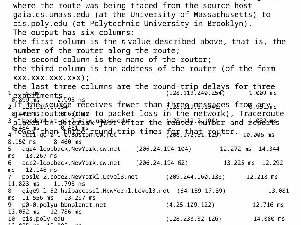
Here is an example of the output of the Traceroute program, where the route was being traced from the source host gaia.cs.umass.edu (at the University of Massachusetts) to cis.poly.edu (at Polytechnic University in Brooklyn). The output has six columns:the first column is the n value described above, that is, the number of the router along the route; the second column is the name of the router; the third column is the address of the router (of the form xxx.xxx.xxx.xxx); the last three columns are the round-trip delays for three experiments. If the source receives fewer than three messages from any given router (due to packet loss in the network), Traceroute places an asterisk just after the router number and reports fewer than three round-trip times for that router.

1   cs-gw  (128.119.240.254)   1.009 ms  0.899 ms  0.993 ms2   128.119.3.154   (128.119.3.154)   0.931 ms  0.441 ms  0.651 ms3   border4-rt-gi-l-3.gw.umass.edu  (128.119.2.194)   1.032 ms  0.484 ms 0.451 ms4   acrl-ge-2-l-0.Boston.cw.net  (208.172.51.129)  10.006 ms 8.150 ms 8.460 ms5   agr4-loopback.NewYork.cw.net  (206.24.194.104)   12.272 ms  14.344 ms  13.267 ms6   acr2-loopback.NewYork.cw.net  (206.24.194.62)   13.225 ms  12.292 ms  12.148 ms7   posl0-2.core2.NewYorkl.Level3.net  (209.244.160.133)   12.218 ms  11.823 ms  11.793 ms8   gige9-l-52.hsipaccessl.NewYorkl.Level3.net  (64.159.17.39)   13.081 ms 11.556 ms  13.297 ms9   p0-0.polyu.bbnplanet.net  (4.25.109.122)   12.716 ms 13.052 ms 12.786 ms10  cis.poly.edu   (128.238.32.126)    14.080 ms  13.035 ms  12.802  ms

In the trace above there are nine routers between the source and the destination. Most of these routers have a name, and all of them have addresses. For example, the name of Router 3 is border4-rt-gi-l-3.gw.umass.edu and its address is 128.119.2.194.Looking at the data provided for this same router, we see that in the first of the three trials the round-trip delay between the source and the router was 1.03msec. The round-trip delays for the subsequent two trials were 0.48 and 0.45msec.These round-trip delays include all of the delays just discussed, including transmission delays, propagation delays, router processing delays, and queuing delays. Because the queuing delay is varying with time, the round-trip delay of packet n sent to a router n can actually be longer than the round-trip delay of packet n+1 sent to router n+1. Indeed, note in the example above that the delays to Router 6 appear to be larger than the delays in Router 7. Note that this is an artifact of the measurement process - any packet going to Router 7 must necessarily pass through Router 6.

Want to try out Traceroute for yourself? We highly recommended that you visit http://www.traceroute.org, which provides a Web interface to an extensive of list of sources for route tracing.You choose a source and supply the hostname for any destination. The Traceroute program then does all the work.