1.7 Grid Sifting: Leveling and Crossing Reductionchris/down/GridSifting.pdf · short edges segments of e. The ﬁrst and the last segments are the outer segments and the others the

1.7

Grid Sifting: Leveling and Crossing Reduction

CHRISTIAN BACHMAIER, WOLFGANG BRUNNER, and ANDREAS GLEIßNER,University of Passau

Directed graphs are commonly drawn by the Sugiyama algorithm where first vertices are placed on distincthierarchical levels, and second the vertices on the same level are permuted to reduce the overall number ofcrossings. Separating these two phases simplifies the algorithms but diminishes the quality of the result.

We introduce a combined leveling and crossing reduction algorithm based on sifting, which prioritizes fewcrossings over few levels. It avoids type 2 conflicts, which are crossings of edges whose endpoints are dummyvertices. This helps straightening long edges spanning many levels. The obtained running time is roughlyquadratic in the size of the input graph and independent of dummy vertices.

Categories and Subject Descriptors: F.2.2 [Analysis of Algorithms and Problem Complexity]: Nonnu-merical Algorithms and Problems—Routing and Layout; G.2.2 [Discrete Mathematics]: Graph Theory—Graph algorithms

General Terms: Algorithms, Design, Experimentation, Performance, Theory

Additional Key Words and Phrases: Crossing reduction, global approach, level graphs, no dummy vertices,Sugiyama framework

ACM Reference Format:Bachmaier, C., Brunner, W., Gleißner, A. 2011. Grid Sifting: Leveling and Crossing Reduction. ACM J. Exp.Algor. 17, 1, Article 1.7 (September 2012), 23 pages.DOI = 10.1145/2133803.2345682 http://doi.acm.org/10.1145/2133803.2345682

1. INTRODUCTIONThe Sugiyama framework [Sugiyama et al. 1981] is the standard drawing algorithmfor directed graphs. It displays them in a hierarchical manner and operates in fourphases: cycle removal (reverse appropriate edges to eliminate cycles), leveling (assignvertices to levels which define the y-coordinates and introduce dummy vertices on longedges), crossing reduction (permute the vertices on the levels), and coordinate assign-ment (assign x-coordinates to the vertices according to some aesthetic criteria). Typicalapplications are schedules, UML diagrams, and flow charts.

There are many different leveling and crossing reduction algorithms. Traditionalleveling methods minimize the number of levels by the longest path method [Kauf-mann and Wagner 2001], by the Coffman/Graham algorithm with a predefined maxi-mum number of vertices per level (width) [Coffman and Graham 1972], or by Gansneret al.’s [1993] ILP minimizing the sum of the edge lengths. The common solution fork-level crossing minimization is a reduction to the still NP-hard [Eades and Wormald1994] one-sided 2-level crossing minimization problem, which is repeatedly solved

This work is supported by the Deutsche Forschungsgemeinschaft (DFG) under grant Br835/15-1 and grantBr835/15-2.Author’s address: Faculty of Informatics and Mathematics, Innstr. 33, University of Passau, 94030 Passau,Germany.Permission to make digital or hard copies of part or all of this work for personal or classroom use is grantedwithout fee provided that copies are not made or distributed for profit or commercial advantage and thatcopies show this notice on the first page or initial screen of a display along with the full citation. Copyrightsfor components of this work owned by others than ACM must be honored. Abstracting with credit is per-mitted. To copy otherwise, to republish, to post on servers, to redistribute to lists, or to use any componentof this work in other works requires prior specific permission and/or a fee. Permissions may be requestedfrom Publications Dept., ACM, Inc., 2 Penn Plaza, Suite 701, New York, NY 10121-0701 USA, fax +1 (212)869-0481, or [email protected].© 2012 ACM 1084-6654/2012/09-ART1.7 $15.00DOI 10.1145/2133803.2345682 http://doi.acm.org/10.1145/2133803.2345682

ACM Journal of Experimental Algorithmics, Vol. 17, No. 1, Article 1.7, Publication date: September 2012.

1.7:2 C. Bachmaier et al.

1 2

3 4

(a) Two levels.

1 2

3

4

(b) Three levels.

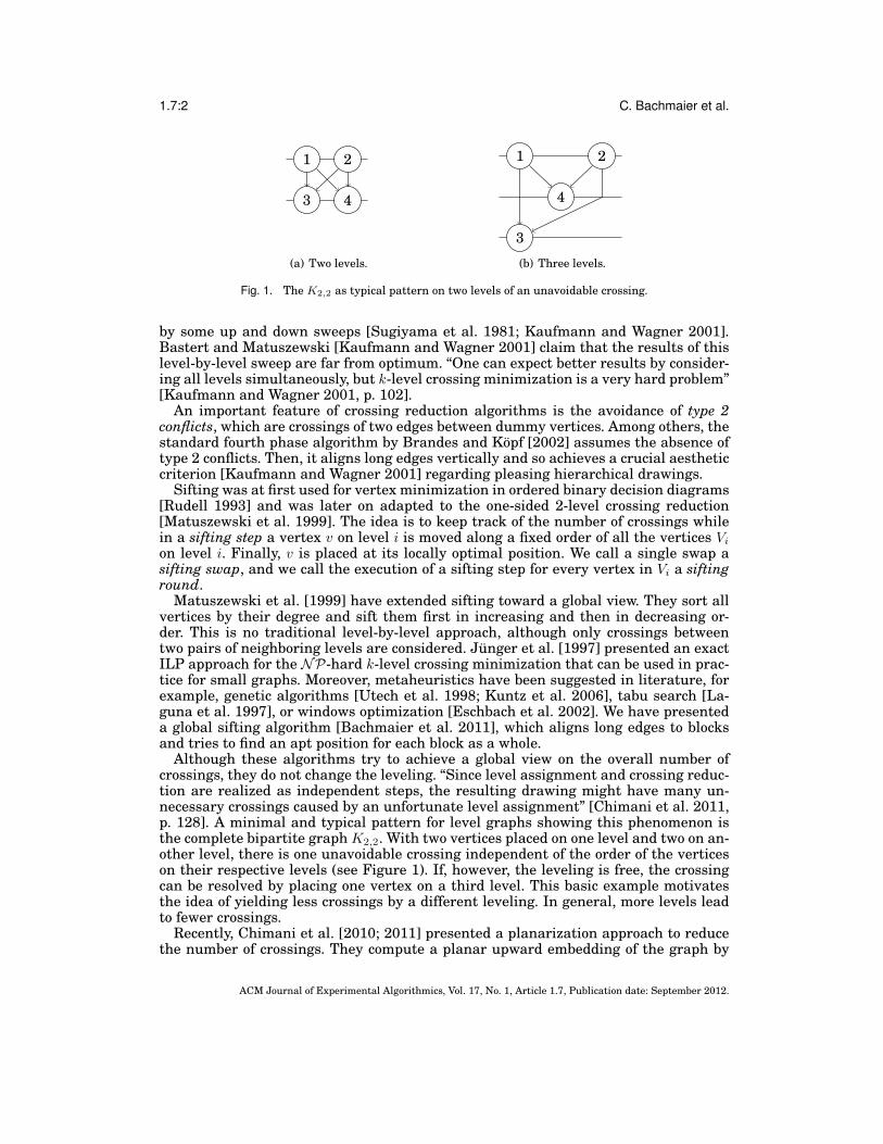
Fig. 1. The K2,2 as typical pattern on two levels of an unavoidable crossing.

by some up and down sweeps [Sugiyama et al. 1981; Kaufmann and Wagner 2001].Bastert and Matuszewski [Kaufmann and Wagner 2001] claim that the results of thislevel-by-level sweep are far from optimum. “One can expect better results by consider-ing all levels simultaneously, but k-level crossing minimization is a very hard problem”[Kaufmann and Wagner 2001, p. 102].

An important feature of crossing reduction algorithms is the avoidance of type 2conflicts, which are crossings of two edges between dummy vertices. Among others, thestandard fourth phase algorithm by Brandes and Kopf [2002] assumes the absence oftype 2 conflicts. Then, it aligns long edges vertically and so achieves a crucial aestheticcriterion [Kaufmann and Wagner 2001] regarding pleasing hierarchical drawings.

Sifting was at first used for vertex minimization in ordered binary decision diagrams[Rudell 1993] and was later on adapted to the one-sided 2-level crossing reduction[Matuszewski et al. 1999]. The idea is to keep track of the number of crossings whilein a sifting step a vertex v on level i is moved along a fixed order of all the vertices Vion level i. Finally, v is placed at its locally optimal position. We call a single swap asifting swap, and we call the execution of a sifting step for every vertex in Vi a siftinground.

Matuszewski et al. [1999] have extended sifting toward a global view. They sort allvertices by their degree and sift them first in increasing and then in decreasing or-der. This is no traditional level-by-level approach, although only crossings betweentwo pairs of neighboring levels are considered. Junger et al. [1997] presented an exactILP approach for the NP-hard k-level crossing minimization that can be used in prac-tice for small graphs. Moreover, metaheuristics have been suggested in literature, forexample, genetic algorithms [Utech et al. 1998; Kuntz et al. 2006], tabu search [La-guna et al. 1997], or windows optimization [Eschbach et al. 2002]. We have presenteda global sifting algorithm [Bachmaier et al. 2011], which aligns long edges to blocksand tries to find an apt position for each block as a whole.

Although these algorithms try to achieve a global view on the overall number ofcrossings, they do not change the leveling. “Since level assignment and crossing reduc-tion are realized as independent steps, the resulting drawing might have many un-necessary crossings caused by an unfortunate level assignment” [Chimani et al. 2011,p. 128]. A minimal and typical pattern for level graphs showing this phenomenon isthe complete bipartite graph K2,2. With two vertices placed on one level and two on an-other level, there is one unavoidable crossing independent of the order of the verticeson their respective levels (see Figure 1). If, however, the leveling is free, the crossingcan be resolved by placing one vertex on a third level. This basic example motivatesthe idea of yielding less crossings by a different leveling. In general, more levels leadto fewer crossings.

Recently, Chimani et al. [2010; 2011] presented a planarization approach to reducethe number of crossings. They compute a planar upward embedding of the graph by


Grid Sifting: Leveling and Crossings Reduction 1.7:3

adding dummy vertices where two edges would cross. This embedding is leveled re-specting the given orders of the adjacency lists. Then, the number of at most O(∣V ∣)levels is reduced by compacting the drawing. The algorithm needs O(∣E∣5) time andstill O(∣E∣3) = O(∣V ∣3) time for planar input graphs.

In this article we propose a new leveling and crossing reduction technique that com-bines both phases in a natural way. We extend global sifting [Bachmaier et al. 2011]to grid sifting such that the blocks are not only sifted “horizontally” on their levelsbut also “vertically” on all suitable levels and prioritize the crossing reduction over theleveling. The algorithm yields better results than traditional heuristics. It avoids type2 conflicts and runs in roughly quadratic time in the size of the input graph.

2. PRELIMINARIESWe suppose that a directed graph without self-loops has passed through the cycle re-moval phase and has been assigned an initial leveling. The outcome is a k-level graphG = (V,E,φ), where φ∶V → {1,2, . . . , k} is a surjective level assignment of the ver-tices with φ(u) < φ(v) for each edge (u, v) ∈ E. For an edge e = (u, v) ∈ E we definespan(e) ∶= φ(v) − φ(u). An edge e is short if span(e) = 1 and long otherwise. A graph isproper if all edges are short.

The traditional approach is to make each level graph proper by adding span(e) − 1dummy vertices for each edge e, which splits e in span(e) many short edges. Let G′ =(V ′,E′, φ′) denote the proper version of G. As in Brandes and Kopf [2002], we callshort edges segments of e. The first and the last segments are the outer segments andthe others the inner segments. Inner segments connect two dummy vertices. For a(level) embedded proper level graph, the vertices on each level are ordered from left toright. In an embedded level graph, two segments are conflicting if they cross or sharea vertex. Conflicts are of type 0, 1, or 2 if they are induced by 0, 1, or 2 inner segments,respectively.

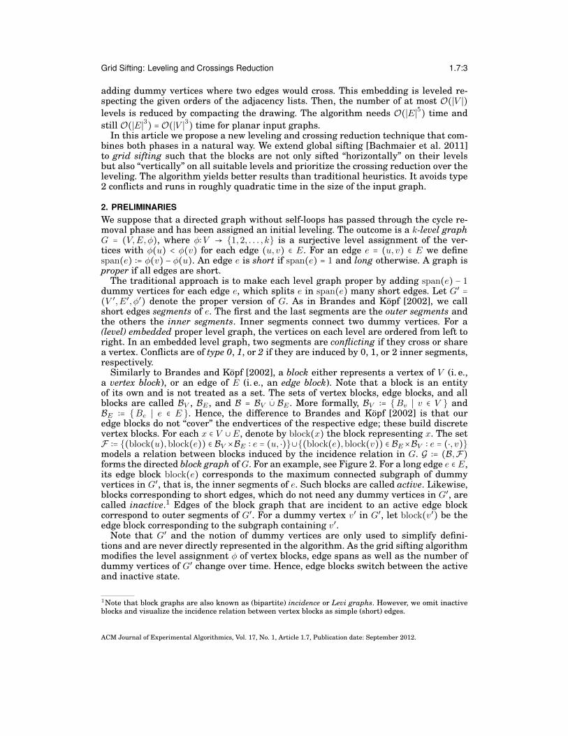
Similarly to Brandes and Kopf [2002], a block either represents a vertex of V (i. e.,a vertex block), or an edge of E (i. e., an edge block). Note that a block is an entityof its own and is not treated as a set. The sets of vertex blocks, edge blocks, and allblocks are called BV , BE , and B = BV

.∪ BE . More formally, BV ∶= {Bv ∣ v ∈ V } andBE ∶= {Be ∣ e ∈ E }. Hence, the difference to Brandes and Kopf [2002] is that ouredge blocks do not “cover” the endvertices of the respective edge; these build discretevertex blocks. For each x ∈ V ∪E, denote by block(x) the block representing x. The setF ∶= {(block(u),block(e)) ∈ BV ×BE ∶ e = (u, ⋅)}∪{(block(e),block(v)) ∈ BE×BV ∶ e = (⋅, v)}models a relation between blocks induced by the incidence relation in G. G ∶= (B,F)forms the directed block graph ofG. For an example, see Figure 2. For a long edge e ∈ E,its edge block block(e) corresponds to the maximum connected subgraph of dummyvertices in G′, that is, the inner segments of e. Such blocks are called active. Likewise,blocks corresponding to short edges, which do not need any dummy vertices in G′, arecalled inactive.1 Edges of the block graph that are incident to an active edge blockcorrespond to outer segments of G′. For a dummy vertex v′ in G′, let block(v′) be theedge block corresponding to the subgraph containing v′.

Note that G′ and the notion of dummy vertices are only used to simplify defini-tions and are never directly represented in the algorithm. As the grid sifting algorithmmodifies the level assignment φ of vertex blocks, edge spans as well as the number ofdummy vertices of G′ change over time. Hence, edge blocks switch between the activeand inactive state.

1Note that block graphs are also known as (bipartite) incidence or Levi graphs. However, we omit inactiveblocks and visualize the incidence relation between vertex blocks as simple (short) edges.



1

2

3

4

5

B

D

3E

u

v

x

y

z

w

A

C

(a) The edge (u, v) spans multiple levels such thatits edge block B represents a path of three dummyvertices.

1

2

3

D

3E

u

v w

A

C

(b) The edge (u, v) is short, which results in an in-active edge block B.

Fig. 2. Example for the proper version G′ of a graph G and its block graph G = ({A,B,C,D,E},{(A,B),(B,C), (A,D), (D,E)}) with two different levelings. The white circles are vertices of G, while the black aredummy vertices of G′. Blocks are shown as rectangles.

Due to technical reasons explained later, most vertex blocks lie on even levels.If an odd level number is not assigned to any vertex block, the level is nonexis-tent. In G′, there is no need to create dummy vertices for that level number. Letnext+(l) (next−(l), respectively) be the next existent level after (before) level l. Ablock is defined to use a level if a (dummy) vertex of the corresponding subgraphin G′ is assigned to this level. Let levels(B) be the set of all levels used by blockB. We define φ(B) ∶= min levels(B) (φ(B) ∶= max levels(B), respectively) as the top-most (bottommost) level used by B. For each vertex block B = block(v), φ(B) =φ(B) = φ(B) ∶= φ(v) holds. An active edge block B = block((u, v)) uses the lev-els φ(B) = next+(φ(u)),next+(next+(φ(u))), . . . ,next−(φ(v)) = φ(B). For inactive edgeblocks B, the set levels(B) is empty.

We introduce l-neighbors of (especially edge) blocks to address parts of these blocksas if the dummy vertices were existent. If (u, v) is any segment in G′ and l = φ(u),we call block(v) an l-neighbor of block(u) in direction “+”. Likewise we call block(u) anl + 1-neighbor of block(v) in direction “−”. Note that if additionally block(u),block(v) ∈BV , then, ignoring the inactive edge block in between, u is a φ(v)-neighbor of v and,accordingly, v is a φ(u)-neighbor of u. For each block B, direction d ∈ {+,−}, and levell ∈ levels(B), we define Nd(B, l) to be the set of all l-neighbors of B in direction d. For anedge block B, Nd(B, l) contains exactly one element. Note that if φ(B) < l < φ(B), thenNd(B, l) = {B}, so that an edge block can be its own l-neighbor. For the perspectiveusing dummy vertices, let v be the dummy vertex of an edge block B on level l. Then,the l-neighbor of B in direction d is the block of the neighbor of v in direction d, whichis either B or an adjacent vertex block. For an example, see Figure 2. In Figure 2(a),the edge (u, v) is long such that the proper version of the graph contains three dummyvertices x, y, and z. They are represented by the edge block B. The 1-neighbors of Ain “+”-direction, N+(A,1), are B and D, since they contain x and w, the immediatesuccessors of u. y is the dummy vertex of B on level 3. It has an edge to the dummy



1 2

4

3

5

Fig. 3. Example of a 4-level graph.

vertex z, which also belongs to B. Thus, the set of 3-neighbors of B in “+”-directionconsists of B itself, that is, N+(B,3) = {B}. In Figure 2(b), the edge (u, v) is short.Thus, the edge block representing (u, v) disappears and is inactive. The proper graphreflects this by u and v connected by an edge. Consequently, N+(A,1) = {C,D}. Foreach vertex block B, we define Nd(B) ∶= Nd(B,φ(B)), as B uses only one level. LetB be an arbitrarily ordered list of all blocks and let π∶B → {0, . . . , ∣B∣ − 1} assign eachblock its current position in this order. Note that the drawing of a short edge (u, v)is independent of π(block((u, v))), since block((u, v)) is inactive. In Figure 2(a), B ={A,B,C,D,E} with π(C) < π(B) < π(A) < π(D) < π(E) = 4. The same ordering fits toFigure 2(b). We call the pair E = (π,φ) a level embedding of the graph.

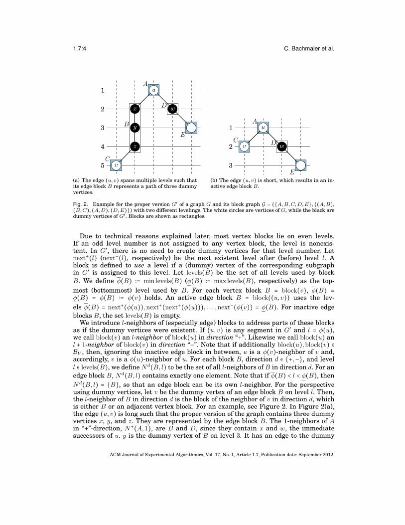
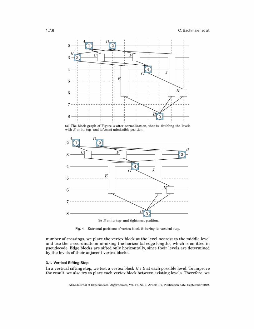
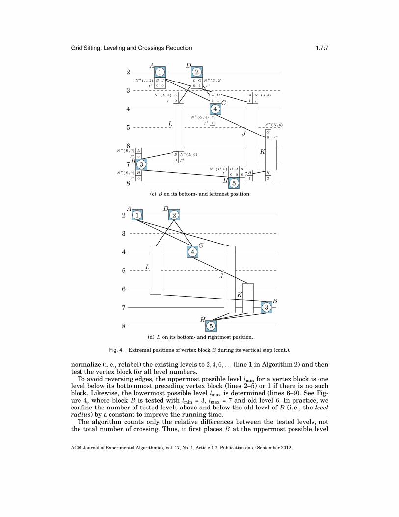
See Figure 3 for another example of a graph G with five vertices and six edges. InFigure 4(a) each of its vertices is represented by a vertex block, and five active edgeblocks are shown. In contrast to Figure 2, we now do not use any dummy verticesin the block graph G of G. The edge (2,3) is short in Figure 4(a), and hence its edgeblock is inactive and not visualized. Levels 5 and 7 are nonexistent (dashed). Thus,next+(4) = 6 and next−(8) = 6. Let J be the edge block of the edge (1,5). Then, levels(J) ={3,4,6}, φ(J) = 3, φ(J) = 6,N+(J,3) = {J},N+(J,4) = {J}, and N+(J,6) = {block(5)} ={H}. Furthermore, N+(D) = {B,F} in Figure 4(a) (ignoring the currently inactive edgeblock L = block(2,3)) and N+(D) = {L,G} in Figure 4(c) (as level 3 is nonexistent,F = block(2,4) is inactive).

3. GRID SIFTINGWe extend our approach of global sifting [Bachmaier et al. 2011] and try to find opti-mal positions for each (vertex) block on all levels. We use a two-dimensional grid onwhich we place each vertex block (see Figure 4(a)). The edge blocks span the levelsbetween their incident vertex blocks and represent the dummy vertices of each edge.Each block has a unique x-coordinate on the grid, which is given by the order of B. Asan initialization, we use an arbitrary leveling and a random permutation of B.

If a given ordering should only be improved in a postprocessing step, a straightfor-ward initialization strategy is to topologically sort the blocks according to the orderingson the levels from left to right in O(∣V ∣+ ∣E∣). Our experiments showed that a good ini-tial ordering of the blocks leads to better results. However, these can also be achievedby one or two additional sifting rounds.

Finding an optimal position for a vertex block basically consists of two nested loops.The outer loop, called a vertical step, iterates over all levels the vertex can use withoutreversing an incident edge. In the inner loop, called a horizontal step, all positions ofthe vertex block on the current level are tested. In the end, the vertex block is placedon the level and position causing the minimal number of crossings. See Algorithm 1 forthe entry to the detailed description. If there are several positions causing the same



2

3

4

5

6

7

8

C

E

F

J

K

3B

1A

2D

4G

5H

(a) The block graph of Figure 3 after normalization, that is, doubling the levelswith B on its top- and leftmost admissible position.

2

3

4

5

6

7

8

C

E

F

J

K

3B

1A

2D

4G

5H

(b) B on its top- and rightmost position.

Fig. 4. Extremal positions of vertex block B during its vertical step.

number of crossings, we place the vertex block at the level nearest to the middle leveland use the x-coordinate minimizing the horizontal edge lengths, which is omitted inpseudocode. Edge blocks are sifted only horizontally, since their levels are determinedby the levels of their adjacent vertex blocks.

3.1. Vertical Sifting StepIn a vertical sifting step, we test a vertex block B ∈ B at each possible level. To improvethe result, we also try to place each vertex block between existing levels. Therefore, we



2

3

4

5

6

7

8

L

J

K

3B

1A

2D

4G

5H

N+(A,2)I+

G

0

J

0

N+(D,2)I+

L

0

G

1

N−(L,4)I−

D

0

N+(L,6)I+

B

0

A

0

D

1

N+(G,4)I+

K

0

N−(J,4)I−

A

1

H

1

N−(K,6)

I−G

0

H

2

N−(H,8)I−

B

0

J

0

K

0

N−(B,7)I−

L

0

N+(B,7)I+

H

0

(c) B on its bottom- and leftmost position.

2

3

4

5

6

7

8

L

J

K

3B

1A

2D

4G

5H

(d) B on its bottom- and rightmost position.

Fig. 4. Extremal positions of vertex block B during its vertical step (cont.).

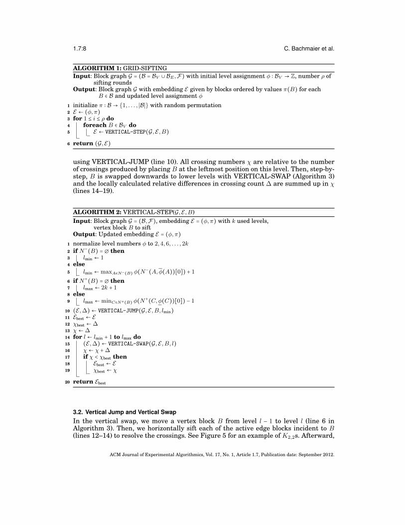
normalize (i. e., relabel) the existing levels to 2,4,6, . . . (line 1 in Algorithm 2) and thentest the vertex block for all level numbers.

To avoid reversing edges, the uppermost possible level lmin for a vertex block is onelevel below its bottommost preceding vertex block (lines 2–5) or 1 if there is no suchblock. Likewise, the lowermost possible level lmax is determined (lines 6–9). See Fig-ure 4, where block B is tested with lmin = 3, lmax = 7 and old level 6. In practice, weconfine the number of tested levels above and below the old level of B (i. e., the levelradius) by a constant to improve the running time.

The algorithm counts only the relative differences between the tested levels, notthe total number of crossing. Thus, it first places B at the uppermost possible level



ALGORITHM 1: GRID-SIFTINGInput: Block graph G = (B = BV ∪ BE ,F) with initial level assignment φ ∶ BV → Z, number ρ of

sifting roundsOutput: Block graph G with embedding E given by blocks ordered by values π(B) for each

B ∈ B and updated level assignment φ1 initialize π ∶ B → {1, . . . , ∣B∣} with random permutation2 E ← (φ,π)3 for 1 ≤ i ≤ ρ do4 foreach B ∈ BV do5 E ← VERTICAL-STEP(G,E ,B)

6 return (G,E)

using VERTICAL-JUMP (line 10). All crossing numbers χ are relative to the numberof crossings produced by placing B at the leftmost position on this level. Then, step-by-step, B is swapped downwards to lower levels with VERTICAL-SWAP (Algorithm 3)and the locally calculated relative differences in crossing count ∆ are summed up in χ(lines 14–19).

ALGORITHM 2: VERTICAL-STEP(G,E ,B)Input: Block graph G = (B,F), embedding E = (φ,π) with k used levels,

vertex block B to siftOutput: Updated embedding E = (φ,π)

1 normalize level numbers φ to 2,4,6, . . . ,2k2 if N−

(B) = ∅ then3 lmin ← 14 else5 lmin ←maxA∈N−(B) φ(N

−(A,φ(A))[0]) + 1

6 if N+(B) = ∅ then

7 lmax ← 2k + 18 else9 lmax ←minC∈N+(B) φ(N

+(C,φ(C))[0]) − 1

10 (E ,∆)← VERTICAL-JUMP(G,E ,B, lmin)

11 Ebest ← E

12 χbest ←∆13 χ←∆14 for l ← lmin + 1 to lmax do15 (E ,∆)← VERTICAL-SWAP(G,E ,B, l)16 χ← χ +∆17 if χ < χbest then18 Ebest ← E

19 χbest ← χ

20 return Ebest

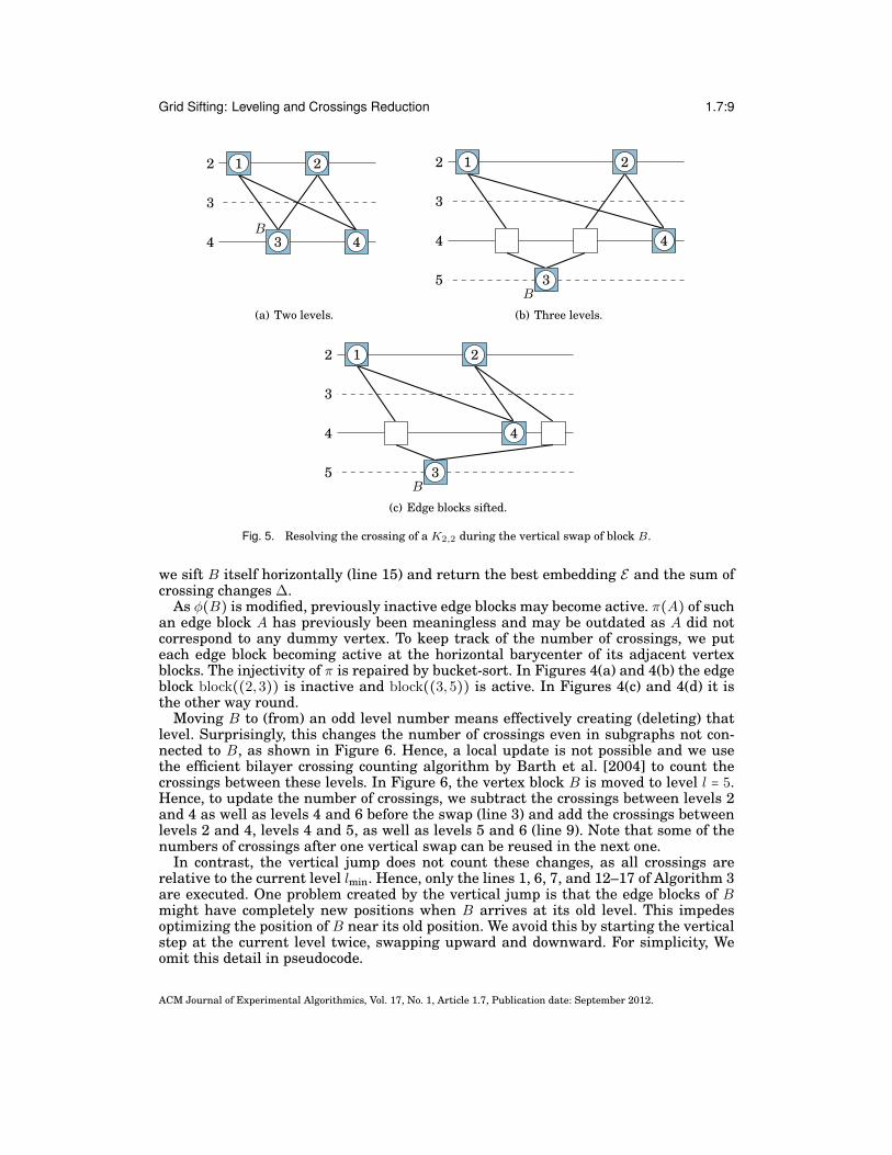
3.2. Vertical Jump and Vertical SwapIn the vertical swap, we move a vertex block B from level l − 1 to level l (line 6 inAlgorithm 3). Then, we horizontally sift each of the active edge blocks incident to B(lines 12–14) to resolve the crossings. See Figure 5 for an example of K2,2s. Afterward,



2

3

4

1 2

3B

4

(a) Two levels.

2

3

4

5

1 2

4

3B

(b) Three levels.

2

3

4

5

1 2

4

3B

(c) Edge blocks sifted.

Fig. 5. Resolving the crossing of a K2,2 during the vertical swap of block B.

we sift B itself horizontally (line 15) and return the best embedding E and the sum ofcrossing changes ∆.

As φ(B) is modified, previously inactive edge blocks may become active. π(A) of suchan edge block A has previously been meaningless and may be outdated as A did notcorrespond to any dummy vertex. To keep track of the number of crossings, we puteach edge block becoming active at the horizontal barycenter of its adjacent vertexblocks. The injectivity of π is repaired by bucket-sort. In Figures 4(a) and 4(b) the edgeblock block((2,3)) is inactive and block((3,5)) is active. In Figures 4(c) and 4(d) it isthe other way round.

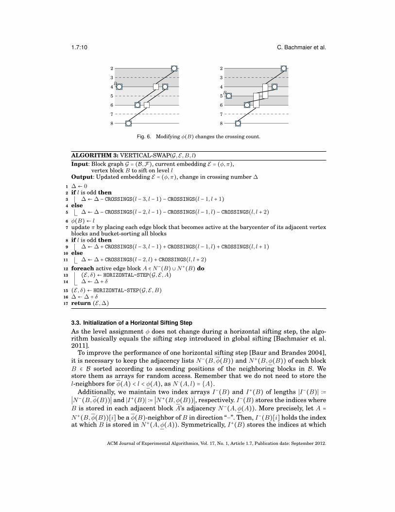
Moving B to (from) an odd level number means effectively creating (deleting) thatlevel. Surprisingly, this changes the number of crossings even in subgraphs not con-nected to B, as shown in Figure 6. Hence, a local update is not possible and we usethe efficient bilayer crossing counting algorithm by Barth et al. [2004] to count thecrossings between these levels. In Figure 6, the vertex block B is moved to level l = 5.Hence, to update the number of crossings, we subtract the crossings between levels 2and 4 as well as levels 4 and 6 before the swap (line 3) and add the crossings betweenlevels 2 and 4, levels 4 and 5, as well as levels 5 and 6 (line 9). Note that some of thenumbers of crossings after one vertical swap can be reused in the next one.

In contrast, the vertical jump does not count these changes, as all crossings arerelative to the current level lmin. Hence, only the lines 1, 6, 7, and 12–17 of Algorithm 3are executed. One problem created by the vertical jump is that the edge blocks of Bmight have completely new positions when B arrives at its old level. This impedesoptimizing the position of B near its old position. We avoid this by starting the verticalstep at the current level twice, swapping upward and downward. For simplicity, Weomit this detail in pseudocode.



2

3

4

5

6

7

8

B

2

3

4

5

6

7

8

B

Fig. 6. Modifying φ(B) changes the crossing count.

ALGORITHM 3: VERTICAL-SWAP(G,E ,B, l)Input: Block graph G = (B,F), current embedding E = (φ,π),

vertex block B to sift on level lOutput: Updated embedding E = (φ,π), change in crossing number ∆

1 ∆← 02 if l is odd then3 ∆←∆ − CROSSINGS(l − 3, l − 1) − CROSSINGS(l − 1, l + 1)4 else5 ∆←∆ − CROSSINGS(l − 2, l − 1) − CROSSINGS(l − 1, l) − CROSSINGS(l, l + 2)

6 φ(B)← l7 update π by placing each edge block that becomes active at the barycenter of its adjacent vertex

blocks and bucket-sorting all blocks8 if l is odd then9 ∆←∆ + CROSSINGS(l − 3, l − 1) + CROSSINGS(l − 1, l) + CROSSINGS(l, l + 1)

10 else11 ∆←∆ + CROSSINGS(l − 2, l) + CROSSINGS(l, l + 2)

12 foreach active edge block A ∈ N−(B) ∪N+

(B) do13 (E , δ)← HORIZONTAL-STEP(G,E ,A)

14 ∆←∆ + δ

15 (E , δ)← HORIZONTAL-STEP(G,E ,B)

16 ∆←∆ + δ17 return (E ,∆)

3.3. Initialization of a Horizontal Sifting StepAs the level assignment φ does not change during a horizontal sifting step, the algo-rithm basically equals the sifting step introduced in global sifting [Bachmaier et al.2011].

To improve the performance of one horizontal sifting step [Baur and Brandes 2004],it is necessary to keep the adjacency lists N−(B,φ(B)) and N+(B,φ(B)) of each blockB ∈ B sorted according to ascending positions of the neighboring blocks in B. Westore them as arrays for random access. Remember that we do not need to store thel-neighbors for φ(A) < l < φ(A), as N ⋅(A, l) = {A}.

Additionally, we maintain two index arrays I−(B) and I+(B) of lengths ∣I−(B)∣ ∶=∣N−(B,φ(B))∣ and ∣I+(B)∣ ∶= ∣N+(B,φ(B))∣, respectively. I−(B) stores the indices whereB is stored in each adjacent block A’s adjacency N−(A,φ(A)). More precisely, let A =N+(B,φ(B))[i] be a φ(B)-neighbor of B in direction “−”. Then, I−(B)[i] holds the indexat which B is stored in N+(A,φ(A)). Symmetrically, I+(B) stores the indices at which



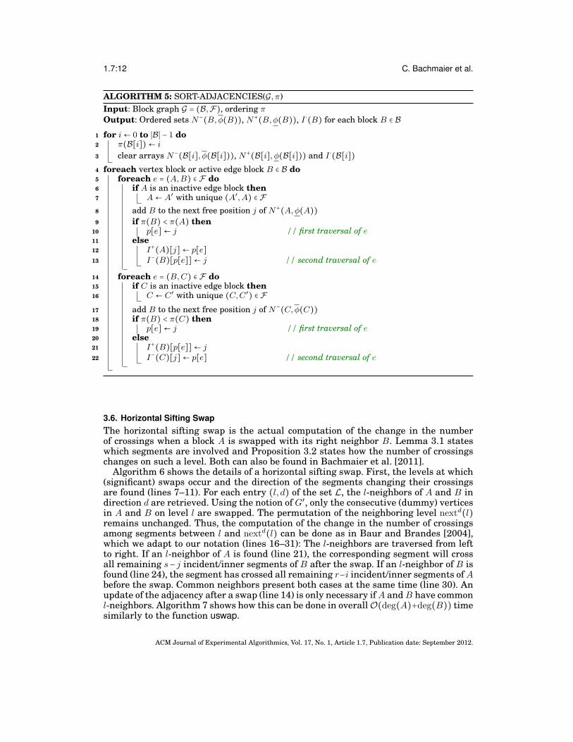
B is stored in the adjacency N−(A,φ(A)) of each adjacent block A. See Figure 4(c) foran example. The creation of the four arrays for each block (line 7 of Algorithm 4) canbe done in O(∣E∣) time by traversing B once. See Algorithm 5 for details.

3.4. Sorting and Updating the AdjacenciesWith Algorithm 5, we build up the sorted adjacency of each block before each horizontalstep. We traverse each block B in the current order of B and add B to the next freeposition j of the cleared adjacency array N+(A,φ(A)) (N−(C,φ(C))) of each incomingφ(B)-neighbor A (outgoing φ(B)-neighbor C). Both values for I+(A) and I−(B) (I+(B)and I−(C)) and their positions are only known after the second traversal of a segmente. Thus, we cache the first array position j as an attribute p of e. Let v ∈ V ′ be a dummyvertex of an edge block B with φ(v) = l. We explicitly do not update any outgoing l-neighbor adjacency of v if φ(B) ≤ l < φ(B) and no incoming adjacency of v if φ(B) < l ≤φ(B). For performance reasons, these vertices and arrays are only implicit and wouldonly contain one element N ⋅(B, l)[0] = B. Thus, associated values “I ⋅(B, l)” are notneeded in Algorithm 7. For B, only two arrays, I−(B) and I+(B), remain, representingthe position of B in its incident vertex blocks.

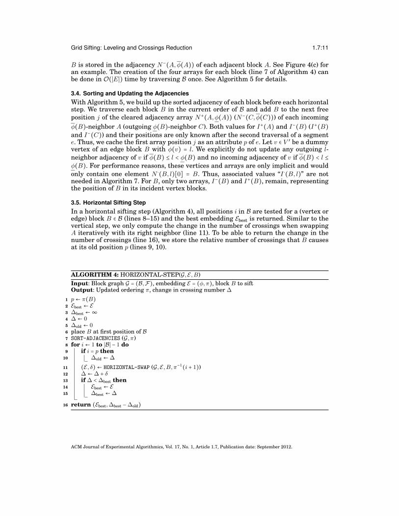
3.5. Horizontal Sifting StepIn a horizontal sifting step (Algorithm 4), all positions i in B are tested for a (vertex oredge) block B ∈ B (lines 8–15) and the best embedding Ebest is returned. Similar to thevertical step, we only compute the change in the number of crossings when swappingA iteratively with its right neighbor (line 11). To be able to return the change in thenumber of crossings (line 16), we store the relative number of crossings that B causesat its old position p (lines 9, 10).

ALGORITHM 4: HORIZONTAL-STEP(G,E ,B)Input: Block graph G = (B,F), embedding E = (φ,π), block B to siftOutput: Updated ordering π, change in crossing number ∆

1 p← π(B)

2 Ebest ← E

3 ∆best ←∞

4 ∆← 05 ∆old ← 06 place B at first position of B7 SORT-ADJACENCIES (G, π)8 for i← 1 to ∣B∣ − 1 do9 if i = p then

10 ∆old ←∆

11 (E , δ)← HORIZONTAL-SWAP (G,E ,B, π−1(i + 1))12 ∆←∆ + δ13 if ∆ < ∆best then14 Ebest ← E

15 ∆best ←∆

16 return (Ebest,∆best −∆old)



ALGORITHM 5: SORT-ADJACENCIES(G, π)Input: Block graph G = (B,F), ordering πOutput: Ordered sets N−

(B,φ(B)), N+(B,φ(B)), I ⋅(B) for each block B ∈ B

1 for i← 0 to ∣B∣ − 1 do2 π(B[i])← i

3 clear arrays N−(B[i], φ(B[i])), N+

(B[i], φ(B[i])) and I ⋅(B[i])

4 foreach vertex block or active edge block B ∈ B do5 foreach e = (A,B) ∈ F do6 if A is an inactive edge block then7 A← A′ with unique (A′,A) ∈ F

8 add B to the next free position j of N+(A,φ(A))

9 if π(B) < π(A) then10 p[e]← j // first traversal of e11 else12 I+(A)[j]← p[e]13 I−(B)[p[e]]← j // second traversal of e

14 foreach e = (B,C) ∈ F do15 if C is an inactive edge block then16 C ← C′ with unique (C,C ′

) ∈ F

17 add B to the next free position j of N−(C,φ(C))

18 if π(B) < π(C) then19 p[e]← j // first traversal of e20 else21 I+(B)[p[e]]← j22 I−(C)[j]← p[e] // second traversal of e

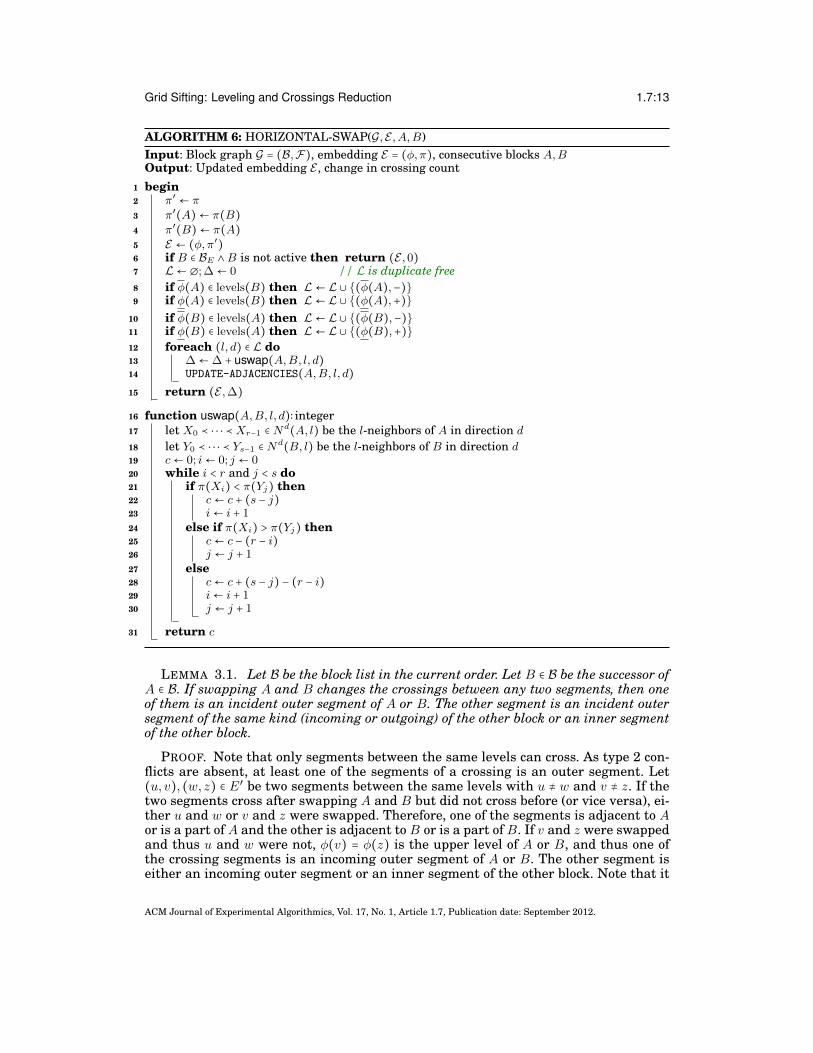
3.6. Horizontal Sifting SwapThe horizontal sifting swap is the actual computation of the change in the numberof crossings when a block A is swapped with its right neighbor B. Lemma 3.1 stateswhich segments are involved and Proposition 3.2 states how the number of crossingschanges on such a level. Both can also be found in Bachmaier et al. [2011].

Algorithm 6 shows the details of a horizontal sifting swap. First, the levels at which(significant) swaps occur and the direction of the segments changing their crossingsare found (lines 7–11). For each entry (l, d) of the set L, the l-neighbors of A and B indirection d are retrieved. Using the notion of G′, only the consecutive (dummy) verticesin A and B on level l are swapped. The permutation of the neighboring level nextd(l)remains unchanged. Thus, the computation of the change in the number of crossingsamong segments between l and nextd(l) can be done as in Baur and Brandes [2004],which we adapt to our notation (lines 16–31): The l-neighbors are traversed from leftto right. If an l-neighbor of A is found (line 21), the corresponding segment will crossall remaining s− j incident/inner segments of B after the swap. If an l-neighbor of B isfound (line 24), the segment has crossed all remaining r−i incident/inner segments ofAbefore the swap. Common neighbors present both cases at the same time (line 30). Anupdate of the adjacency after a swap (line 14) is only necessary ifA andB have commonl-neighbors. Algorithm 7 shows how this can be done in overallO(deg(A)+deg(B)) timesimilarly to the function uswap.



ALGORITHM 6: HORIZONTAL-SWAP(G,E ,A,B)Input: Block graph G = (B,F), embedding E = (φ,π), consecutive blocks A,BOutput: Updated embedding E , change in crossing count

1 begin2 π′ ← π3 π′(A)← π(B)

4 π′(B)← π(A)

5 E ← (φ,π′)6 if B ∈ BE ∧B is not active then return (E ,0)7 L← ∅; ∆← 0 // L is duplicate free8 if φ(A) ∈ levels(B) then L← L ∪ {(φ(A),−)}9 if φ(A) ∈ levels(B) then L← L ∪ {(φ(A),+)}

10 if φ(B) ∈ levels(A) then L← L ∪ {(φ(B),−)}11 if φ(B) ∈ levels(A) then L← L ∪ {(φ(B),+)}

12 foreach (l, d) ∈ L do13 ∆←∆ + uswap(A,B, l, d)14 UPDATE-ADJACENCIES(A,B, l, d)

15 return (E ,∆)

16 function uswap(A,B, l, d)∶ integer17 let X0 ≺ ⋅ ⋅ ⋅ ≺Xr−1 ∈ Nd

(A, l) be the l-neighbors of A in direction d18 let Y0 ≺ ⋅ ⋅ ⋅ ≺ Ys−1 ∈ Nd

(B, l) be the l-neighbors of B in direction d19 c← 0; i← 0; j ← 020 while i < r and j < s do21 if π(Xi) < π(Yj) then22 c← c + (s − j)23 i← i + 124 else if π(Xi) > π(Yj) then25 c← c − (r − i)26 j ← j + 127 else28 c← c + (s − j) − (r − i)29 i← i + 130 j ← j + 1

31 return c

LEMMA 3.1. Let B be the block list in the current order. Let B ∈ B be the successor ofA ∈ B. If swapping A and B changes the crossings between any two segments, then oneof them is an incident outer segment of A or B. The other segment is an incident outersegment of the same kind (incoming or outgoing) of the other block or an inner segmentof the other block.

PROOF. Note that only segments between the same levels can cross. As type 2 con-flicts are absent, at least one of the segments of a crossing is an outer segment. Let(u, v), (w, z) ∈ E′ be two segments between the same levels with u ≠ w and v ≠ z. If thetwo segments cross after swapping A and B but did not cross before (or vice versa), ei-ther u and w or v and z were swapped. Therefore, one of the segments is adjacent to Aor is a part of A and the other is adjacent to B or is a part of B. If v and z were swappedand thus u and w were not, φ(v) = φ(z) is the upper level of A or B, and thus one ofthe crossing segments is an incoming outer segment of A or B. The other segment iseither an incoming outer segment or an inner segment of the other block. Note that it



cannot be an outgoing outer segment of this block because then neither u and w nor vand z would have been swapped. The other case of swapping u and w instead of v andz is symmetric.

PROPOSITION 3.2. Let B be the block list in the current order. Let B ∈ B be thesuccessor of A ∈ B. Let i and j be the two levels framing the incoming outer segmentsof A, the other three cases are symmetric. If there is a segment (u, v) between i andj, which is either an incoming outer segment of B or an inner segment of B, then theincoming segments of A starting at a block left of block(u) cross (u, v) after the swapof A and B only, the segments starting at block(u) never cross (u, v), and the segmentsstarting right of block(u) cross (u, v) before the swap only. There are no other changesof crossings due to Lemma 3.1.

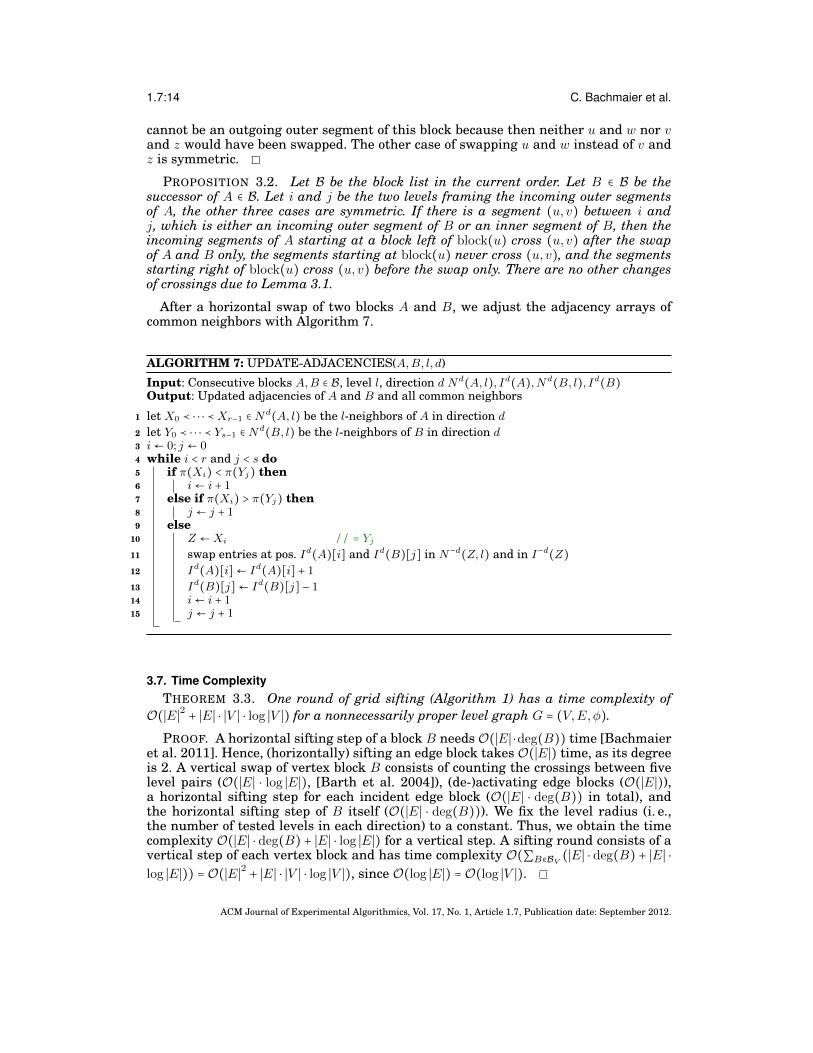
After a horizontal swap of two blocks A and B, we adjust the adjacency arrays ofcommon neighbors with Algorithm 7.

ALGORITHM 7: UPDATE-ADJACENCIES(A,B, l, d)

Input: Consecutive blocks A,B ∈ B, level l, direction d Nd(A, l), Id(A),Nd

(B, l), Id(B)

Output: Updated adjacencies of A and B and all common neighbors

1 let X0 ≺ ⋅ ⋅ ⋅ ≺Xr−1 ∈ Nd(A, l) be the l-neighbors of A in direction d

2 let Y0 ≺ ⋅ ⋅ ⋅ ≺ Ys−1 ∈ Nd(B, l) be the l-neighbors of B in direction d

3 i← 0; j ← 04 while i < r and j < s do5 if π(Xi) < π(Yj) then6 i← i + 17 else if π(Xi) > π(Yj) then8 j ← j + 19 else

10 Z ←Xi // = Yj

11 swap entries at pos. Id(A)[i] and Id(B)[j] in N−d(Z, l) and in I−d(Z)

12 Id(A)[i]← Id(A)[i] + 1

13 Id(B)[j]← Id(B)[j] − 114 i← i + 115 j ← j + 1

3.7. Time ComplexityTHEOREM 3.3. One round of grid sifting (Algorithm 1) has a time complexity of

O(∣E∣2 + ∣E∣ ⋅ ∣V ∣ ⋅ log ∣V ∣) for a nonnecessarily proper level graph G = (V,E,φ).PROOF. A horizontal sifting step of a block B needs O(∣E∣ ⋅deg(B)) time [Bachmaier

et al. 2011]. Hence, (horizontally) sifting an edge block takes O(∣E∣) time, as its degreeis 2. A vertical swap of vertex block B consists of counting the crossings between fivelevel pairs (O(∣E∣ ⋅ log ∣E∣), [Barth et al. 2004]), (de-)activating edge blocks (O(∣E∣)),a horizontal sifting step for each incident edge block (O(∣E∣ ⋅ deg(B)) in total), andthe horizontal sifting step of B itself (O(∣E∣ ⋅ deg(B))). We fix the level radius (i. e.,the number of tested levels in each direction) to a constant. Thus, we obtain the timecomplexity O(∣E∣ ⋅ deg(B) + ∣E∣ ⋅ log ∣E∣) for a vertical step. A sifting round consists of avertical step of each vertex block and has time complexity O(∑B∈BV

(∣E∣ ⋅ deg(B) + ∣E∣ ⋅log ∣E∣)) = O(∣E∣2 + ∣E∣ ⋅ ∣V ∣ ⋅ log ∣V ∣), since O(log ∣E∣) = O(log ∣V ∣).



1

2

3

4

5

6

1 2

3 4 5

6 7

8 9

10 11

12 13 14

(a) Cuts from left to right.

1

2

3

4

1 3 4 2

6 9 7 5

10 8 11

12 13 14

(b) Compacted.

Fig. 7. Vertical compaction.

The time complexity is O(∣E∣2) for dense graphs with ∣E∣ ≥ ∣V ∣ log ∣V ∣. Our experi-ments show that the counting of the crossings can be neglected in practice. The timecomplexity increases to O(∣E∣2 ⋅ ∣V ∣ + ∣E∣ ⋅ ∣V ∣2 ⋅ log ∣V ∣) in total using an unfixed levelradius.

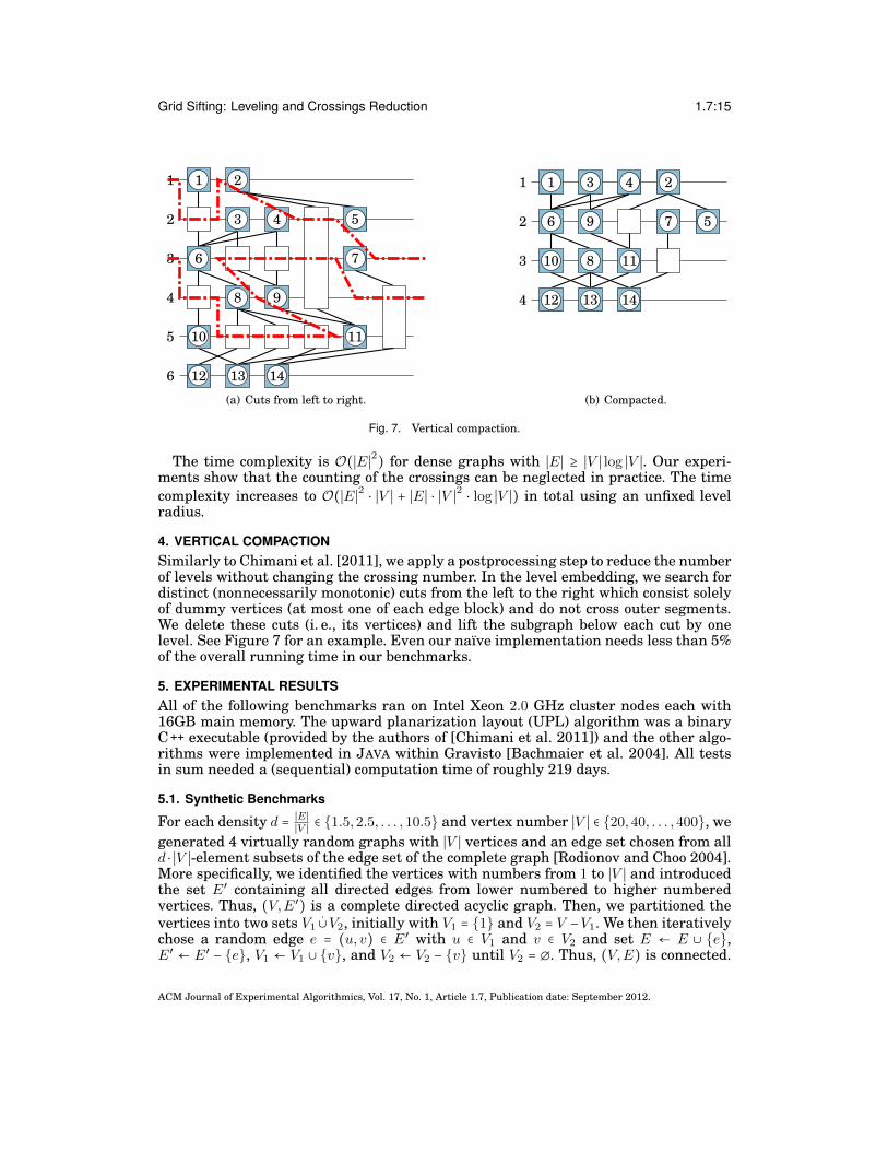
4. VERTICAL COMPACTIONSimilarly to Chimani et al. [2011], we apply a postprocessing step to reduce the numberof levels without changing the crossing number. In the level embedding, we search fordistinct (nonnecessarily monotonic) cuts from the left to the right which consist solelyof dummy vertices (at most one of each edge block) and do not cross outer segments.We delete these cuts (i. e., its vertices) and lift the subgraph below each cut by onelevel. See Figure 7 for an example. Even our naıve implementation needs less than 5%of the overall running time in our benchmarks.

5. EXPERIMENTAL RESULTSAll of the following benchmarks ran on Intel Xeon 2.0 GHz cluster nodes each with16GB main memory. The upward planarization layout (UPL) algorithm was a binaryC++ executable (provided by the authors of [Chimani et al. 2011]) and the other algo-rithms were implemented in JAVA within Gravisto [Bachmaier et al. 2004]. All testsin sum needed a (sequential) computation time of roughly 219 days.

5.1. Synthetic Benchmarks

For each density d = ∣E∣∣V ∣ ∈ {1.5,2.5, . . . ,10.5} and vertex number ∣V ∣ ∈ {20,40, . . . ,400}, wegenerated 4 virtually random graphs with ∣V ∣ vertices and an edge set chosen from alld ⋅ ∣V ∣-element subsets of the edge set of the complete graph [Rodionov and Choo 2004].More specifically, we identified the vertices with numbers from 1 to ∣V ∣ and introducedthe set E′ containing all directed edges from lower numbered to higher numberedvertices. Thus, (V,E′) is a complete directed acyclic graph. Then, we partitioned thevertices into two sets V1

.∪V2, initially with V1 = {1} and V2 = V −V1. We then iterativelychose a random edge e = (u, v) ∈ E′ with u ∈ V1 and v ∈ V2 and set E ← E ∪ {e},E′ ← E′ − {e}, V1 ← V1 ∪ {v}, and V2 ← V2 − {v} until V2 = ∅. Thus, (V,E) is connected.



Then, we iteratively chose a random edge e from the remaining edges in E′ and setE′ ← E′ − {e} and E ← E ∪ {e}. In the latter step, whenever ∣E∣ = d ⋅ ∣V ∣, we stopped andobtained the benchmark graph (V,E).2

We used the state of the art Coffman/Graham algorithm with level width 1, yieldinga virtually random injective initial leveling φ ∶ V → {1, . . . , ∣V ∣}, in order to give the al-gorithms some freedom to place vertices. As a side effect, φ also imposes an ascendingtopological ordering on the vertices. We compared the algorithms iterative one-sided2-level barycenter (BC) [Kaufmann and Wagner 2001], global sifting (GlS) [Bachmaieret al. 2011], upward planarization layout (UPL) [Chimani et al. 2011], and our grid sift-ing algorithm with the level radii 3 (GrS3), 10 (GrS10) and unconfined (GrS*). GrS21uses radius 21 but odd (i. e., new) levels only. Hence, GrS21 holds the invariant of hav-ing only one vertex per level. Then, the new levels adjacent to the current level of eachvertex can be omitted as well, and GrS21 tests the same number of levels as GrS10.

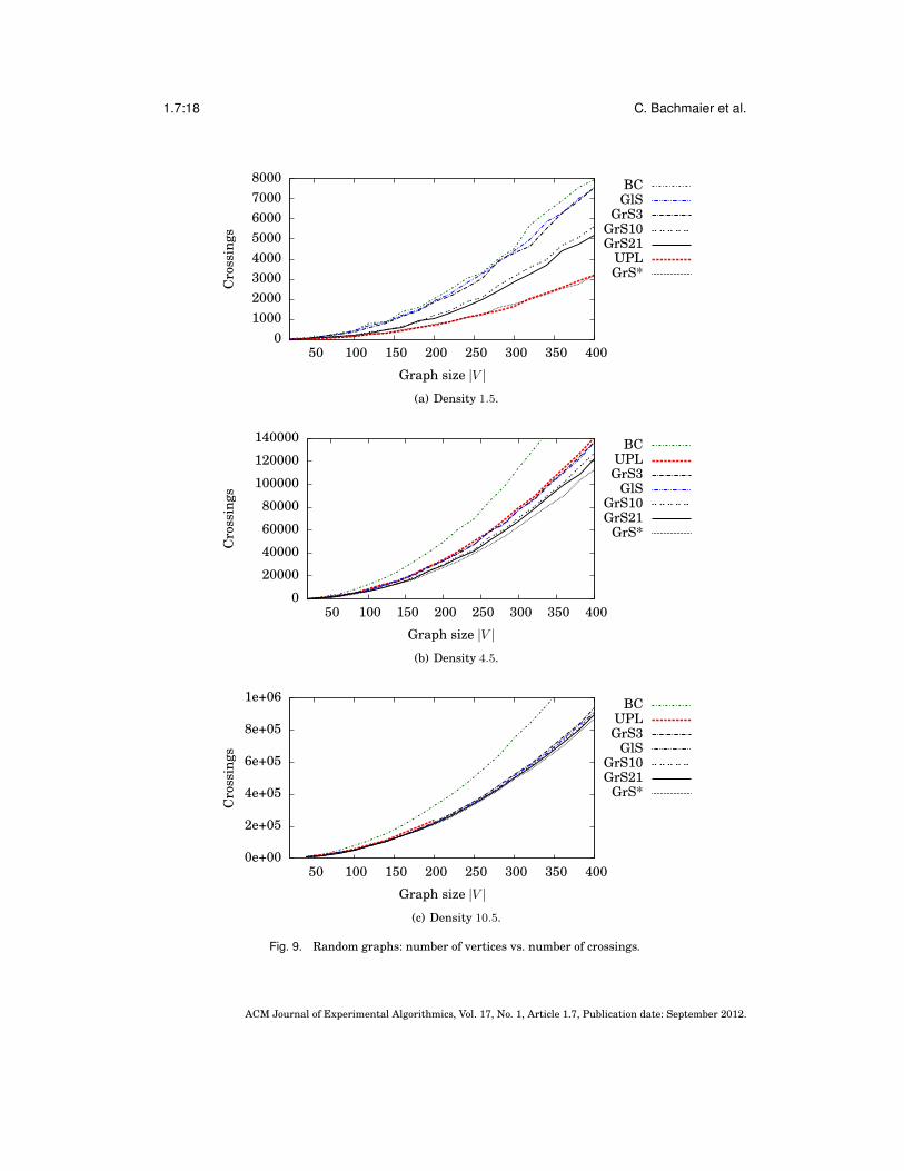
We executed eight rounds for each grid sifting variant, since then there is no furthersignificant improvement in the number of crossings. We applied UPL 20 times on eachinput to choose the best result. Clearly, BC and GlS are the fastest algorithms byfar, but they cannot change the leveling. To ensure that their results do not sufferfrom saving running time, we execute (actually unreasonable) 400 sweeps and siftingrounds, respectively.

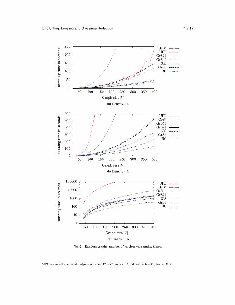
As UPL is slower than our grid sifting algorithms (Figure 10), we could not testUPL for graphs with a density greater than 4.5 and more than 200 vertices. The run-ning time (Figure 8) of the grid sifting variants with restricted level radius are rathercomparable to GlS, whereas BC is always fastest.

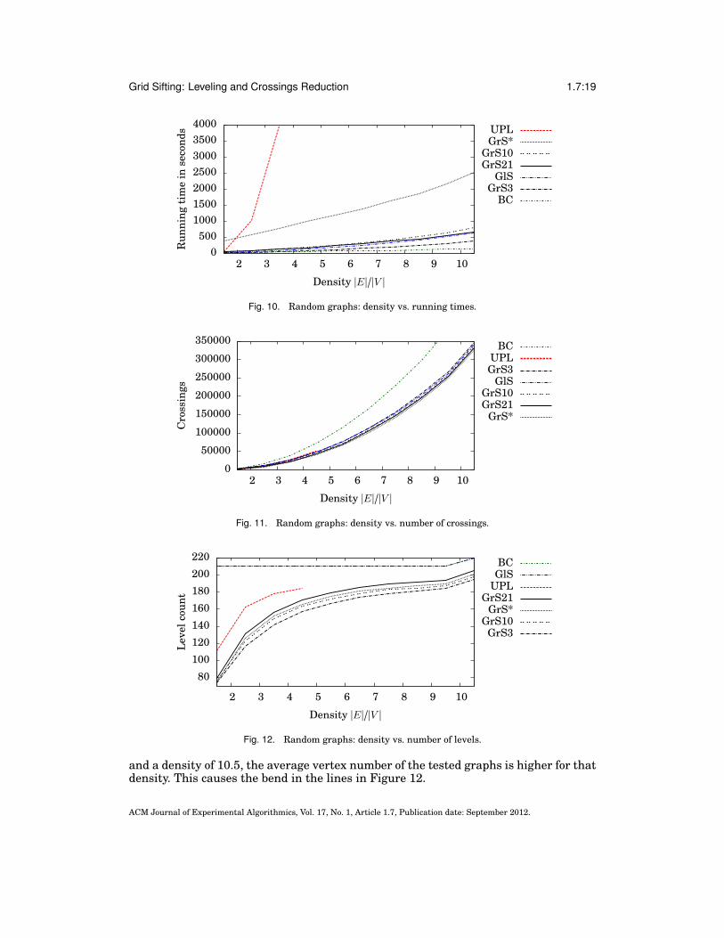
Note the crossings of the lines GrS10, GrS21, and GlS in Figure 8(c), which, at firstglance, contradict the same asymptotic runtime ofO(∣E∣2). Compared to GrS10, GrS21uses the double level radius, that is, it tries to place vertices at levels that are up todouble the distance of their original level, but it tests only odd levels. Consequently,GrS10 and GrS21 perform the same number of horizontal steps in large graphs. Then,GrS10 is slightly slower because of the different relative amount of runtime requiredby counting the bilayer crossings. However, as in small graphs the number of actuallytested levels is effectively restricted by the total number of levels rather than the levelradius, GrS21 is faster than GrS10 for graphs with less than 80 vertices. A similarargument applies to GlS, which corresponds to grid sifting with level radius 0, that is,it omits vertical swaps. GrS21 is faster than GlS for small graphs by performing lessrounds, but it is slower once the number of actually tested levels converges to 21 asthe graph size increases. As there are no graphs with 20 vertices and a density of 10.5,the benchmarks in Figure 8(c) start at 40.

Figure 9 shows the obtained quality of the algorithms in terms of crossings at dif-ferent densities. As expected, the higher the level radius is chosen, the less crossingsremain. Compared to that, an increased number of rounds for GlS does not pay out.BC is qualitatively inferior.

Figures 10–12 compare the performance of the algorithms with the density of thegraphs. Clearly, the values shown in Figure 10 are dominated by the running timefor the large instances. For a similar benchmark using graphs with a fixed number ofvertices, see Figure 13. As a further consequence of the absence graphs with 20 vertices

2The generators used are included within the source code of Gravisto [Bachmaier et al. 2004]. Theprimary Java classes are org.graffiti.plugins.algorithms.sugiyama.gridsifting.benchmark.RandomPAand RandomPA2, which contain further instructions for their usage. The employed graphs generated with arandom (but for reproducibility hard-coded) seed can be obtained from the Graph Archive [Bachmaier et al.2012] under keyword “Grid Sifting”.



0

50

100

150

200

250

50 100 150 200 250 300 350 400

Run

ning

tim

ein

seco

nds

Graph size ∣V ∣

GrS*UPL

GrS21GrS10

GlSGrS3

BC

(a) Density 1.5.

0

100

200

300

400

500

600

50 100 150 200 250 300 350 400

Run

ning

tim

ein

seco

nds

Graph size ∣V ∣

UPLGrS*

GrS10GrS21

GlSGrS3

BC

(b) Density 4.5.

1

10

100

1000

10000

100000

50 100 150 200 250 300 350 400

Run

ning

tim

ein

seco

nds

Graph size ∣V ∣

UPLGrS*

GrS10GrS21

GlSGrS3

BC

(c) Density 10.5.

Fig. 8. Random graphs: number of vertices vs. running times.



010002000300040005000600070008000

50 100 150 200 250 300 350 400

Cro

ssin

gs

Graph size ∣V ∣

BCGlS

GrS3GrS10GrS21

UPLGrS*

(a) Density 1.5.

0

20000

40000

60000

80000

100000

120000

140000

50 100 150 200 250 300 350 400

Cro

ssin

gs

Graph size ∣V ∣

BCUPLGrS3

GlSGrS10GrS21

GrS*

(b) Density 4.5.

0e+00

2e+05

4e+05

6e+05

8e+05

1e+06

50 100 150 200 250 300 350 400

Cro

ssin

gs

Graph size ∣V ∣

BCUPLGrS3

GlSGrS10GrS21

GrS*

(c) Density 10.5.

Fig. 9. Random graphs: number of vertices vs. number of crossings.



0500

1000150020002500300035004000

2 3 4 5 6 7 8 9 10

Run

ning

tim

ein

seco

nds

Density ∣E∣/∣V ∣

UPLGrS*

GrS10GrS21

GlSGrS3

BC

Fig. 10. Random graphs: density vs. running times.

0

50000

100000

150000

200000

250000

300000

350000

2 3 4 5 6 7 8 9 10

Cro

ssin

gs


BCUPLGrS3

GlSGrS10GrS21

GrS*

Fig. 11. Random graphs: density vs. number of crossings.

80

100

120

140

160

180

200

220

2 3 4 5 6 7 8 9 10

Lev

elco

unt


BCGlS

UPLGrS21

GrS*GrS10

GrS3

Fig. 12. Random graphs: density vs. number of levels.

and a density of 10.5, the average vertex number of the tested graphs is higher for thatdensity. This causes the bend in the lines in Figure 12.



0

5

10

15

20

25

30

35

1.6 1.8 2 2.2 2.4

Run

ning

tim

ein

seco

nds


GrS*UPL

GrS10GrS21

GlSGrS3

BC

Fig. 13. Random graphs with 100 vertices: density vs. running times.

0

500

1000

1500

2000

2500

3000

1.6 1.8 2 2.2 2.4

Cro

ssin

gs


BCGlS

GrS3UPL

GrS10GrS21

GrS*

Fig. 14. Random graphs with 100 vertices: density vs. number of crossings.

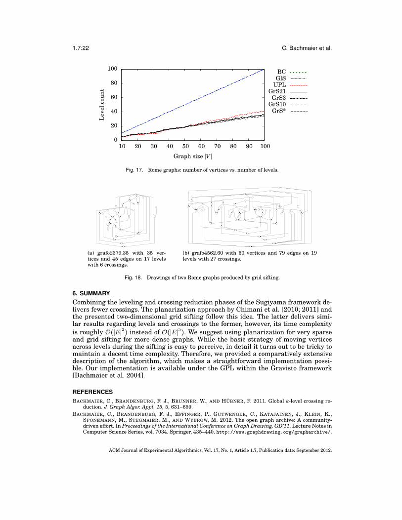
In Figure 11, yet at a density of 2.5, all grid sifting variants give less crossings thanUPL, with throughout a lower number of levels (Figure 12). GrS21 is a good trade-off between running time and result. The Wilcoxon signed rank test [Wilcoxon 1945]indicates with a confidence of 99% that GrS21 yields 8.1% less crossings than UPL forgraphs with density 2.5, 13.1% for density 4.5, and 9.1% for density 10.5. Aggregatingall tested densities, GrS21 yields 11.8% less crossings than UPL. The number of levelsis in both algorithms rather high (Figure 12), which is a consequence of optimizing thenumber of crossings first.

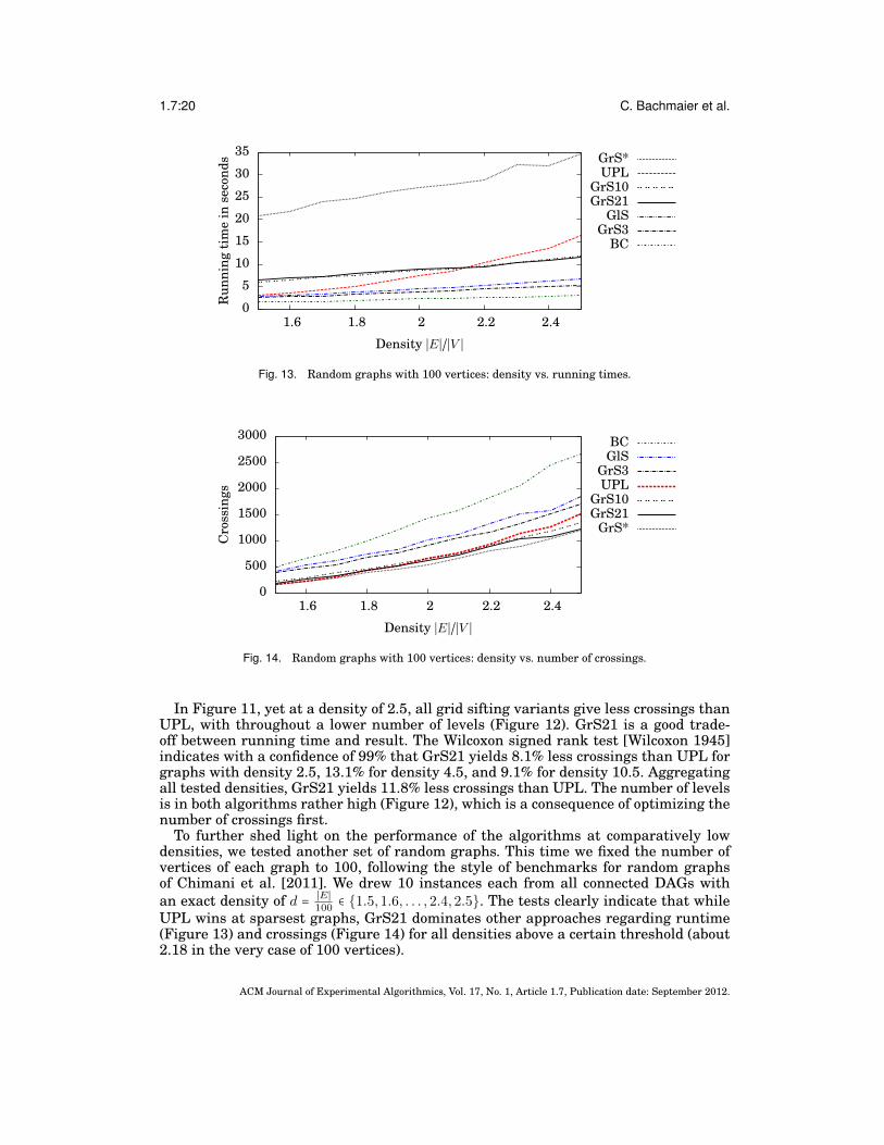
To further shed light on the performance of the algorithms at comparatively lowdensities, we tested another set of random graphs. This time we fixed the number ofvertices of each graph to 100, following the style of benchmarks for random graphsof Chimani et al. [2011]. We drew 10 instances each from all connected DAGs withan exact density of d = ∣E∣

100∈ {1.5,1.6, . . . ,2.4,2.5}. The tests clearly indicate that while

UPL wins at sparsest graphs, GrS21 dominates other approaches regarding runtime(Figure 13) and crossings (Figure 14) for all densities above a certain threshold (about2.18 in the very case of 100 vertices).



02468

101214161820

10 20 30 40 50 60 70 80 90 100

Run

ning

tim

ein

seco

nds

Graph size ∣V ∣

GrS*GrS21GrS10

UPLGlS

GrS3BC

Fig. 15. Rome graphs: number of vertices vs. running times.

0

50

100

150

200

250

300

10 20 30 40 50 60 70 80 90 100

Cro

ssin

gs

Graph size ∣V ∣

BCGlS

GrS3GrS10GrS21

GrS*UPL

Fig. 16. Rome graphs: number of vertices vs. number of crossings.

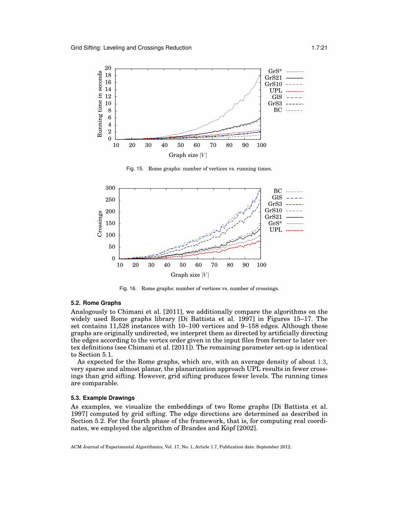
5.2. Rome GraphsAnalogously to Chimani et al. [2011], we additionally compare the algorithms on thewidely used Rome graphs library [Di Battista et al. 1997] in Figures 15–17. Theset contains 11,528 instances with 10–100 vertices and 9–158 edges. Although thesegraphs are originally undirected, we interpret them as directed by artificially directingthe edges according to the vertex order given in the input files from former to later ver-tex definitions (see Chimani et al. [2011]). The remaining parameter set-up is identicalto Section 5.1.

As expected for the Rome graphs, which are, with an average density of about 1.3,very sparse and almost planar, the planarization approach UPL results in fewer cross-ings than grid sifting. However, grid sifting produces fewer levels. The running timesare comparable.

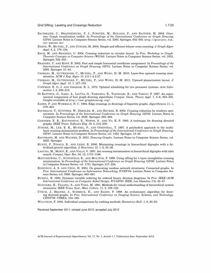
5.3. Example DrawingsAs examples, we visualize the embeddings of two Rome graphs [Di Battista et al.1997] computed by grid sifting. The edge directions are determined as described inSection 5.2. For the fourth phase of the framework, that is, for computing real coordi-nates, we employed the algorithm of Brandes and Kopf [2002].



0

20

40

60

80

100

10 20 30 40 50 60 70 80 90 100

Lev

elco

unt

Graph size ∣V ∣

BCGlS

UPLGrS21

GrS3GrS10

GrS*

Fig. 17. Rome graphs: number of vertices vs. number of levels.

(a) grafo2379.35 with 35 ver-tices and 45 edges on 17 levelswith 6 crossings.

(b) grafo4562.60 with 60 vertices and 79 edges on 19levels with 27 crossings.

Fig. 18. Drawings of two Rome graphs produced by grid sifting.

6. SUMMARYCombining the leveling and crossing reduction phases of the Sugiyama framework de-livers fewer crossings. The planarization approach by Chimani et al. [2010; 2011] andthe presented two-dimensional grid sifting follow this idea. The latter delivers simi-lar results regarding levels and crossings to the former, however, its time complexityis roughly O(∣E∣2) instead of O(∣E∣5). We suggest using planarization for very sparseand grid sifting for more dense graphs. While the basic strategy of moving verticesacross levels during the sifting is easy to perceive, in detail it turns out to be tricky tomaintain a decent time complexity. Therefore, we provided a comparatively extensivedescription of the algorithm, which makes a straightforward implementation possi-ble. Our implementation is available under the GPL within the Gravisto framework[Bachmaier et al. 2004].

REFERENCESBACHMAIER, C., BRANDENBURG, F. J., BRUNNER, W., AND HUBNER, F. 2011. Global k-level crossing re-

duction. J. Graph Algor. Appl. 15, 5, 631–659.BACHMAIER, C., BRANDENBURG, F. J., EFFINGER, P., GUTWENGER, C., KATAJAINEN, J., KLEIN, K.,

SPONEMANN, M., STEGMAIER, M., AND WYBROW, M. 2012. The open graph archive: A community-driven effort. In Proceedings of the International Conference on Graph Drawing, GD’11. Lecture Notes inComputer Science Series, vol. 7034. Springer, 435–440. http://www.graphdrawing.org/grapharchive/.



BACHMAIER, C., BRANDENBURG, F. J., FORSTER, M., HOLLEIS, P., AND RAITNER, M. 2004. Grav-isto: Graph visualization toolkit. In Proceedings of the International Conference on Graph Drawing,GD’04. Lecture Notes in Computer Science Series, vol. 3383. Springer, 502–503. http://gravisto.fim.uni-passau.de/.

BARTH, W., MUTZEL, P., AND JUNGER, M. 2004. Simple and efficient bilayer cross counting. J. Graph Algor.Appl. 8, 2, 179–194.

BAUR, M. AND BRANDES, U. 2004. Crossing reduction in circular layout. In Proc. Workshop in Graph-Theoretic Concepts in Computer Science (WG’04). Lecture Notes in Computer Science Series, vol. 3353.Springer, 332–343.

BRANDES, U. AND KOPF, B. 2002. Fast and simple horizontal coordinate assignment. In Proceedings of theInternational Conference on Graph Drawing, GD’01. Lecture Notes in Computer Science Series, vol.2265. Springer, 31–44.

CHIMANI, M., GUTWENGER, C., MUTZEL, P., AND WONG, H.-M. 2010. Layer-free upward crossing mini-mization. ACM J. Exp. Algor. 15, 2.2.1–2.2.27.

CHIMANI, M., GUTWENGER, C., MUTZEL, P., AND WONG, H.-M. 2011. Upward planarization layout. J.Graph Algor. Appl. 15, 1, 127–155.

COFFMAN, E. G. J. AND GRAHAM, R. L. 1972. Optimal scheduling for two processor systems. Acta Infor-matica 1, 3, 200–213.

DI BATTISTA, G., GARG, A., LIOTTA, G., TAMASSIA, R., TASSINARI, E., AND VARGIU, F. 1997. An exper-imental comparison of four graph drawing algorithms. Comput. Geom. Theory Appl. 7, 5–6, 303–325.Graphs available at http://www.graphdrawing.org/.

EADES, P. AND WORMALD, N. C. 1994. Edge crossings in drawings of bipartite graphs. Algorithmica 11, 1,379–403.

ESCHBACH, T., GUNTHER, W., DREXLER, R., AND BECKER, B. 2002. Crossing reduction by windows opti-mization. In Proceedings of the International Conference on Graph Drawing, GD’02. Lecture Notes inComputer Science Series, vol. 2528. Springer, 285–294.

GANSNER, E. R., KOUTSOFIOS, E., NORTH, S., AND VO, K.-P. 1993. A technique for drawing directedgraphs. IEEE Trans. Software Eng. 19, 3, 214–230.

JUNGER, M., LEE, E. K., MUTZEL, P., AND ODENTHAL, T. 1997. A polyhedral approach to the multi-layer crossing minimization problem. In Proceedings of the International Conference on Graph Drawing,GD’97. Lecture Notes in Computer Science Series, vol. 1353. Springer, 13–24.

KAUFMANN, M. AND WAGNER, D. 2001. Drawing Graphs. Lecture Notes in Computer Science Series, vol.2025. Springer.

KUNTZ, P., PINAUD, B., AND LEHN, R. 2006. Minimizing crossings in hierarchical digraphs with a hy-bridized genetic algorithm. J. Heuristics 12, 1–2, 23–26.

LAGUNA, M., MARTI, R., AND VALLS, V. 1997. Arc crossing minimization in hierarchical digraphs with tabusearch. Comput. Oper. Res. 24, 12, 1175–1186.

MATUSZEWSKI, C., SCHONFELD, R., AND MOLITOR, P. 1999. Using sifting for k-layer straightline crossingminimization. In Proceedings of the International Conference on Graph Drawing, GD’99. Lecture Notesin Computer Science Series, vol. 1731. Springer, 217–224.

RODIONOV, A. S. AND CHOO, H. 2004. On generating random network structures: Connected graphs. InProc. International Conference on Information Networking, ICOIN’04. Lecture Notes in Computer Sci-ence Series, vol. 3090. Springer, 483–491.

RUDELL, R. 1993. Dynamic variable ordering for ordered binary decision diagrams. In Proc. IEEE/ACMInternational Conference on Computer Aided Design, ICCAD’93. IEEE, Los Alamitos, CA, 42–47.

SUGIYAMA, K., TAGAWA, S., AND TODA, M. 1981. Methods for visual understanding of hierarchical systemstructures. IEEE Trans. Syst., Man, Cybern. 11, 2, 109–125.

UTECH, J., BRANKE, J., SCHMECK, H., AND EADES, P. 1998. An evolutionary algorithm for draw-ing directed graphs. In Proc. International Conference on Imaging Science, Systems, and Technology,CISST’98. CSREA, 154–160.

WILCOXON, F. 1945. Individual comparisons by ranking methods. Biometrics Bull. 1, 6, 80–83.

Received September 2011; revised June 2012; accepted July 2012


Documents

1.7 Grid Sifting: Leveling and Crossing Reductionchris/down/GridSifting.pdf · short edges segments of e. The ﬁrst and the last segments are the outer segments and the others the