Embed Size (px)
Citation preview

i

ii

POLYNOMIALS
Alain Lascoux
September 16, 2013

ii
Contents
1 Operators on polynomials 71.1 A,B,C,D . . . . . . . . . . . . . . . . . . . . . . . . . . . . . . . 71.2 Reduced decompositions in type A . . . . . . . . . . . . . . . . . 101.3 Acting on polynomials with the symmetric group . . . . . . . . . 111.4 Commutation relations . . . . . . . . . . . . . . . . . . . . . . . . 131.5 Maximal operators for type A . . . . . . . . . . . . . . . . . . . . 191.6 Littlewood’s formulas . . . . . . . . . . . . . . . . . . . . . . . . . 221.7 Yang-Baxter relations . . . . . . . . . . . . . . . . . . . . . . . . . 261.8 Yang-Baxter bases and the Hecke algebra . . . . . . . . . . . . . . 301.9 t1t2-Yang-Baxter bases . . . . . . . . . . . . . . . . . . . . . . . . 361.10 B, C, D action on polynomials . . . . . . . . . . . . . . . . . . . 411.11 Some operators on symmetric functions . . . . . . . . . . . . . . . 461.12 Weyl character formula . . . . . . . . . . . . . . . . . . . . . . . . 511.13 Macdonald Poincaré polynomial . . . . . . . . . . . . . . . . . . . 531.14 Poincaré with descents . . . . . . . . . . . . . . . . . . . . . . . . 57
2 Linear Bases for type A 612.1 Schubert, Grothendieck and Demazure . . . . . . . . . . . . . . . 612.2 Using the y-variables . . . . . . . . . . . . . . . . . . . . . . . . . 642.3 Flag complete and elementary functions . . . . . . . . . . . . . . 652.4 Three scalar products . . . . . . . . . . . . . . . . . . . . . . . . 682.5 Kernels . . . . . . . . . . . . . . . . . . . . . . . . . . . . . . . . . 702.6 Adjoint Schubert and Grothendieck polynomials . . . . . . . . . . 712.7 Bases adjoint to elementary and complete functions . . . . . . . . 722.8 Adjoint key polynomials . . . . . . . . . . . . . . . . . . . . . . . 742.9 Reproducing kernels for Schubert and Grothendieck polynomials . 762.10 Cauchy formula for Schubert . . . . . . . . . . . . . . . . . . . . . 772.11 Cauchy formula for Grothendieck . . . . . . . . . . . . . . . . . . 792.12 Divided differences as scalar products . . . . . . . . . . . . . . . . 802.13 Divided differences in terms of permutations . . . . . . . . . . . . 812.14 Schubert, Grothendieck and Demazure as commutation factors . . 83
iii

iv Contents
2.15 Cauchy formula for key polynomials . . . . . . . . . . . . . . . . . 892.16 π and π-reproducing kernels . . . . . . . . . . . . . . . . . . . . . 912.17 Decompositions in the affine Hecke algebra . . . . . . . . . . . . . 93
3 Properties of Schubert polynomials 973.1 Schubert by vanishing properties . . . . . . . . . . . . . . . . . . 973.2 Multivariate interpolation . . . . . . . . . . . . . . . . . . . . . . 983.3 Permutations versus divided differences . . . . . . . . . . . . . . . 1003.4 Wronskian of symmetric functions . . . . . . . . . . . . . . . . . . 1033.5 Yang-Baxter and Schubert . . . . . . . . . . . . . . . . . . . . . . 1063.6 Distance 1 and multiplication . . . . . . . . . . . . . . . . . . . . 1093.7 Pieri formula for Schubert polynomials . . . . . . . . . . . . . . . 1123.8 Products of Schubert polynomials by operators on y . . . . . . . . 1163.9 Transition for Schubert polynomials . . . . . . . . . . . . . . . . . 1223.10 Branching rules . . . . . . . . . . . . . . . . . . . . . . . . . . . . 1233.11 Vexillary Schubert polynomials . . . . . . . . . . . . . . . . . . . 1263.12 Schubert and hooks . . . . . . . . . . . . . . . . . . . . . . . . . . 1283.13 Stable part of Schubert polynomials . . . . . . . . . . . . . . . . . 1323.14 Schubert and the Littlewood-Richardson rule . . . . . . . . . . . . 135
4 Products and transitions for Grothendieck and Keys 1374.1 Monk formula for type A key polynomials . . . . . . . . . . . . . 1374.2 Product Gv x1 . . . xk . . . . . . . . . . . . . . . . . . . . . . . . . . 1384.3 Product Kv x1 . . . xk . . . . . . . . . . . . . . . . . . . . . . . . . . 1414.4 Relating the two products . . . . . . . . . . . . . . . . . . . . . . 1424.5 Product with (x1 . . . xk)
−1 . . . . . . . . . . . . . . . . . . . . . . 1434.6 More keys: KG polynomials . . . . . . . . . . . . . . . . . . . . . 1454.7 Transitions for Grothendieck polynomials . . . . . . . . . . . . . . 1474.8 Branching and stable G-polynomials . . . . . . . . . . . . . . . . 1504.9 Transitions for Key polynomials . . . . . . . . . . . . . . . . . . . 1524.10 Vexillary polynomials . . . . . . . . . . . . . . . . . . . . . . . . . 1554.11 Grothendieck and Yang-Baxter . . . . . . . . . . . . . . . . . . . 157
5 G1/x and G Grothendieck polynomials 1595.1 Grothendieck in terms of Schubert . . . . . . . . . . . . . . . . . 1595.2 Monk formula for G1/x and G polynomials . . . . . . . . . . . . . 1655.3 Transition for G1/x and G polynomials . . . . . . . . . . . . . . . 1685.4 Action of divided differences on G1/x and G polynomials . . . . . 1695.5 Still more keys: KG polynomials . . . . . . . . . . . . . . . . . . . 1715.6 Graßmannian G1/x and G polynomials . . . . . . . . . . . . . . . 1745.7 Dual Graßmannian Grothendieck polynomials . . . . . . . . . . . 177

Contents v
6 Plactic algebra and the module Schub 1816.1 Tableaux . . . . . . . . . . . . . . . . . . . . . . . . . . . . . . . . 1816.2 Strings . . . . . . . . . . . . . . . . . . . . . . . . . . . . . . . . . 1826.3 Free key polynomials . . . . . . . . . . . . . . . . . . . . . . . . . 1846.4 Embedding of Sym into the plactic algebra . . . . . . . . . . . . . 1856.5 Keys and jeu de taquin on columns . . . . . . . . . . . . . . . . . 1886.6 Keys and keys . . . . . . . . . . . . . . . . . . . . . . . . . . . . . 1896.7 vice-tableaux . . . . . . . . . . . . . . . . . . . . . . . . . . . . . 1906.8 Ehresmann tableaux . . . . . . . . . . . . . . . . . . . . . . . . . 1916.9 Nilplactic monoid and algebra . . . . . . . . . . . . . . . . . . . . 1936.10 Lifting Pol to a submodule of Plac . . . . . . . . . . . . . . . . . 1966.11 Allowable products in Schub . . . . . . . . . . . . . . . . . . . . . 1996.12 Generating function of Schubert polynomials in Schub . . . . . . . 202
7 Schubert and Grothendieck by keys 2057.1 Double keys . . . . . . . . . . . . . . . . . . . . . . . . . . . . . . 2057.2 Magyar’s recursion . . . . . . . . . . . . . . . . . . . . . . . . . . 2107.3 Schubert by nilplactic keys . . . . . . . . . . . . . . . . . . . . . . 2127.4 Schubert by words majorised by reduced decompositions . . . . . 2147.5 Product of a Grothendieck polynomial by a dominant monomial . 2157.6 ASM and monotone triangles . . . . . . . . . . . . . . . . . . . . 218
8 Generating Functions 2218.1 Binary triangles . . . . . . . . . . . . . . . . . . . . . . . . . . . 2218.2 Generating function in the nilplactic algebra . . . . . . . . . . . . 2238.3 Generating function in the NilCoxeter algebra . . . . . . . . . . . 2248.4 Generating function in the 0-Hecke algebra . . . . . . . . . . . . . 2268.5 Hopf decomposition of Schubert and Grothendieck polynomials . . 2278.6 Generating function of G-polynomials . . . . . . . . . . . . . . . . 229
9 Key polynomials for type B,C,D 2319.1 KB, KC , KD . . . . . . . . . . . . . . . . . . . . . . . . . . . . . 2319.2 Scalar products for type B,C,D . . . . . . . . . . . . . . . . . . . 2349.3 Adjointness . . . . . . . . . . . . . . . . . . . . . . . . . . . . . . 2369.4 Symplectic and orthogonal Schur functions . . . . . . . . . . . . . 2389.5 Maximal key polynomials . . . . . . . . . . . . . . . . . . . . . . 2439.6 Symmetrizing further . . . . . . . . . . . . . . . . . . . . . . . . . 2489.7 Finite symplectic Cauchy identity . . . . . . . . . . . . . . . . . . 2509.8 Rectangles and sums of Schur functions . . . . . . . . . . . . . . . 251
10 Macdonald polynomials 25510.1 Interpolation Macdonald polynomials . . . . . . . . . . . . . . . . 25510.2 Recursive generation of Macdonald polynomials . . . . . . . . . . 25710.3 A baby kernel . . . . . . . . . . . . . . . . . . . . . . . . . . . . . 259

vi Contents
10.4 Multiplication by an indeterminate . . . . . . . . . . . . . . . . . 26110.5 Transitions . . . . . . . . . . . . . . . . . . . . . . . . . . . . . . . 26310.6 Symmetric Macdonald polynomials . . . . . . . . . . . . . . . . . 26410.7 Macdonald polynomials versus Key polynomials . . . . . . . . . . 265
11 Hall-Littlewood polynomials 26911.1 From a quadratic form on the Hecke algebra to a quadratic form
on polynomials . . . . . . . . . . . . . . . . . . . . . . . . . . . . 26911.2 Nonsymmetric Hall-Littlewood polynomials . . . . . . . . . . . . 27011.3 Adjoint basis with respect to ( , ) . . . . . . . . . . . . . . . . . . 27111.4 Symmetric Hall-Littlewood polynomials for types A,B,C,D . . . 27211.5 Atoms . . . . . . . . . . . . . . . . . . . . . . . . . . . . . . . . . 27311.6 Q′-Hall-Littlewood functions . . . . . . . . . . . . . . . . . . . . 276
12 Kazhdan-Lusztig bases 27912.1 Basis of the Hecke algebra . . . . . . . . . . . . . . . . . . . . . . 27912.2 Duality . . . . . . . . . . . . . . . . . . . . . . . . . . . . . . . . . 28112.3 Peeling out canonical factors . . . . . . . . . . . . . . . . . . . . . 28312.4 Non-singular permutations . . . . . . . . . . . . . . . . . . . . . . 28512.5 Kazhdan-Lusztig polynomial bases . . . . . . . . . . . . . . . . . 28712.6 Kazhdan-Lusztig and Hall-Littlewood . . . . . . . . . . . . . . . 28912.7 Using key polynomials . . . . . . . . . . . . . . . . . . . . . . . . 29012.8 Parabolic Kazhdan-Lusztig polynomials . . . . . . . . . . . . . . . 29212.9 Graßmannian case . . . . . . . . . . . . . . . . . . . . . . . . . . 29412.10Dual basis and key polynomials . . . . . . . . . . . . . . . . . . . 296
13 Complements 29713.1 The symmetric group . . . . . . . . . . . . . . . . . . . . . . . . . 298
13.1.1 Permutohedron . . . . . . . . . . . . . . . . . . . . . . . . 29813.1.2 Rothe diagram . . . . . . . . . . . . . . . . . . . . . . . . 30013.1.3 Ehresmann-Bruhat order . . . . . . . . . . . . . . . . . . . 301
13.2 t-Schubert polynomials . . . . . . . . . . . . . . . . . . . . . . . . 30513.3 Polynomials under C-action . . . . . . . . . . . . . . . . . . . . . 30913.4 Polynomials under D-action . . . . . . . . . . . . . . . . . . . . . 31313.5 Hecke algebras of types B,C,D . . . . . . . . . . . . . . . . . . . 31513.6 Noncommutative symmetric functions . . . . . . . . . . . . . . . . 324
Bibliography 333

§ 0.0 — CONTENTS
Abstract.We give eight1 linear bases of the ring of polynomials in n indeterminates : Schubert
polynomials, Grothendieck polynomials, flag elementary/complete functions, Demazurecharacters (key polynomials) for types A,B,C,D, Macdonald polynomials.
All these bases are triangular in the basis of monomials, with respect to appropriateorders. We introduce different scalar products and compute the adjoint bases of theprevious polynomials.
We provide recursions (transition formulas) which allow to cut these polynomialsinto smaller ones of the same family.
We recover the multiplicative structure of the ring of polynomials by describing themultiplication by a single variable.
In type A we lift the Schubert polynomials and Demazure characters to the freealgebra.
We recover by symmetrisation Schur functions and symmetric Macdonald polyno-mials in type A, and symplectic and orthogonal Schur functions in types B,C,D.
1In fact, counting adjoint bases and deformations, many more, but the next lucky number,88, seems out of reach for the moment.

Chapter 0 — CONTENTS
Introduction
’oooooo’oooooo
’oooooo’oooooo
’oooooo’oooooo
’oooooo’oooooo
’oooooo’oooooo
’oooooo’oooooo
’oooooo’oooooo
’oooooo’oooooo
Polynomials appeared since the beginnings of algebra, and it may seem thatthere is not much to say, nowadays, about the space of polynomials as a vectorspace. In the case of a single variable x, many linear bases of Pol(x) other thanthe powers of x have been described, starting with the Newton’s interpolationpolynomials. The theory of orthogonal polynomials flourished during the wholeXIXe century, providing many more bases.
In the case of symmetric polynomials, Newton, again, gave a basis of productsof elementary functions. The transition matrices between these functions and themonomial functions were already considered in the XV IIIe century by Vander-monde in particular. Later, the chevalier Faa de Bruno, Cayley, Kostka spentmuch energy computing different other transition matrices. It happens in factthat there is a fundamental basis, the basis of Schur functions. A great majorityof the classical problems in the theory of symmetric functions involve this basis,and leads to a combinatorics of diagrams of partitions and Young tableaux.
The picture is not so bright when one relaxes the condition of symmetry andconsider Pol(x1, . . . , xn) in full generality. In fact, computer algebra systems likeMaple or Mathematica do not know the ring of polynomials in several variableswith coefficients in Z, but only the ring Z[x1] ⊗ Z[x2] ⊗ · · · ⊗ Z[xn]. Since 40years, geometry and representation theory provided a new incentive for describ-ing linear bases of polynomials. The cohomology theory and the K-theory flagmanifolds lead to different bases related to Schubert varieties: Demazure charac-ters, Schubert polynomials, Grothendieck polynomials. Independently, the theoryof orthogonal polynomials, in conjunction with root systems, developed in the di-rection of several variables, with the work of Koornwinder, Macdonald and manyothers.
In these notes, we shall mostly restrict to Schubert polynomials, Grothendieckpolynomials, Demazure characters (key polynomials), Macdonald polynomials. Theseobjects will be obtained using simple operators such as Newton’s divided differ-ences and their deformations. Such operators act on two consecutive variables ata time, say xi, x+1, and commute with multiplication with symmetric functionsin xi, xi+1. Therefore, they are characterized by their action on 1, xi+1 (which isa basis of Pol(xi, xi+1) as a free Sym(xi, xi+1)-module). In type A, computationswill not require more than the rules figuring in the following tableau, which ex-presses the images of 1, xi+1 under different operators, and indicates the relatedpolynomials.

§ 0.0 — CONTENTS
operator si+∂i ∂i πi πi (1−xi+1)∂i Ti
1xi+1
1xi−1
0−1
10
0−xi+1
1xi+xi+1−1
txi
polynoms Jack Schubert Demazure Demazure G MacdonaldGrothendieck Grothendieck Hall−Littlewood
To be complete, we have to add to this list the operators πBn , πCn and πDi in thecase of key polynomials for types B,C,D, and the translation f(x1, . . . , xn) →f(xn/q, x1, . . . , xn−1)(xn−1) in the case of Macdonald polynomials, but this doesnot change the picture: it is remarkable that such simple rules suffice to gen-erate interesting families of polynomials. As a matter of fact, one also needsinitial polynomials. In the case of Demazure characters, one starts with dominantmonomials xλ = xλ1
1 . . . xλnn , λ1 ≥ λ2 ≥ · · · ≥ λn. For Schubert polynomials, oneintroduces another set of variables, and one takes Yλ :=
∏i=1..n,j=1..λi
(xi−yj). ForGrothendieck polynomials, one takes Gλ :=
∏i=1..n,j=1..λi
(1−yjx−1i ), still with the
requirement that λ1 ≥ · · · ≥ λn. In the case of Macdonald polynomials, one needsonly one starting point, which is 1, because the translation operator increasesdegree and allows to generate polynomials of any degree.
Schubert and Macdonald polynomials can also be defined by interpolationproperties. Indeed, to each v ∈ Nn, one associates a spectral vector 〈v〉y (which isa permutation of y1, y2, . . .), and another spectral vector 〈v〉tq (with componentswhich are monomials in t, q). Now the Schubert polynomial Yv and the Macdonaldpolynomial Mv are the only polynomials, up to normalization, of degree d = |v| =v1+ . . . +vn, such that
Yv(〈u〉y
)= 0 & Mv
(〈u〉tq
)= 0 ∀u : |u| ≤ d, u 6= v .
it is easy to check that the vanishing conditions imply a recursion on poly-nomials, the image of a Schubert polynomial under ∂i being another Schubertpolynomial (when it is not 0), and the image of a Macdonald polynomial un-der Ti+c being another Macdonald polynomial (when choosing appropriately theconstant c).
Divided differences are discrete analogues of derivatives. One can thus expecta discrete analogue of themultivariate Taylor formula. In the case of functions of asingle variable, this discrete analogue is the Newton interpolation formula. In themultivariate case, the universal coefficients appearing as coefficients of productsof divided differences are precisely the Schubert polynomials, and this is a directconsequence of their vanishing properties.
In these notes, we have put the emphasis on Grothendieck polynomials, be-cause the literature on this subject is rather scanty , apart from the Graßmanniancase, which is the case where the polynomials are symmetric and can be treatedas deformations of Schur functions. We do not touch the subject of Schubert

Chapter 0 — CONTENTS
polynomials for types B,C,D (see [10, 47, 49, 41, 132, 133]). They require intro-ducing the operation xn → −xn, while, for Demazure characters and K-theory,one must use xn → x−1
n . In type A on the contrary, cohomology and K-theorycan be mixed, operators like πi + ∂i make sense.
Schubert, Grothendieck polynomials and Demazure characters are directly as-sociated to the basis ∂σ : σ ∈ Sn of the Nil Hecke algebra, and to the basisπσ : σ ∈ Sn of the 0-Hecke algebra. We give two more bases, and their ad-joint, of Pol(x1, . . . , xn), corresponding to the basis ∇σ : σ ∈ Sn, and to theKazhdan-Lusztig basis Cσ : σ ∈ Sn of the Hecke algebra.
Linear algebra is not enough, the ring Pol(x1, . . . , xn) has also a multiplicativestructure that one needs to describe. We mostly restrict to multiplication by asingle variable, which is enough to determine the multiplicative structure in eachof the bases that we consider. Already this simple case involves fine properties ofthe Ehresmann-Bruhat order on the symmetric group (or on the affine symmetricgroup in the case of Macdonald polynomials). It is clear, however, that morework should be invested in that direction, the product of two general Schubertpolynomials or two Grothendieck polynomials having, for example, many geomet-rical consequences . Fomin and Kirillov [40] have introduced an quadratic algebrato explain the connections between the Ehresmann-Bruhat order and Schubertcalculus.
Having different bases, one may look for the relations between them. We con-sider the relations between Schubert and Grothendieck, Schubert and Demazure,Macdonald and key polynomials, but this subject is far from being exhausted.
Polynomials can be written uniquely as linear combination of flag elementaryfunctions) (products of the type . . . ei(x1, x2, x3)ej(x1, x2)ek(x1)). Since the nat-ural way to lift an elementary function of degree k in the free algebra is to takethe sum of all strictly decreasing words of degree k, one has therefore a naturalembedding, as a Z-module, of Pol(x1, . . . , xn) in the free algebra on n letters. Weshall rather use a distinguished quotient of the free algebra, the plactic algebraPlac(n), quotient by the relations
cab ≡ acb, bac ≡ bca, baa ≡ aba, bab ≡ bba, a < b < c .
The lift of Sym(x1 . . . , xn) in Plac(n) has now recovered its multiplicative struc-ture, compared to the lift in the free algebra where one must have recourse tooperations like shuffle instead of concatanation of words. In others words, one hasan embedding of Sym(x1 . . . , xn) into a non-commutative algebra, and thereforeany identity on symmetric polynomials translates automatically into a statementin the non-commutative world. Combinatorists will have no difficulty in goingone step further in the translation and use Young tableaux, Dyck paths or non-

§ 0.0 — CONTENTS
intersecting paths instead of mere words. In short, the diagram
Sym
Plac
Pol
sλ →∑T Ev
where the left arrow sends a Schur function sλ onto the sum of all tableaux of shapeλ in the alphabet 1, . . . , n, and Ev is the commutative evaluation, allows to passfrom algebraic identities on symmetric functions to statements about words andtableaux.
Simple transpositions can be lifted to the free algebra, inducing an action ofthe symmetric group on the free algebra. The isobaric divided differences πi canalso be lifted to the free algebra, but they do not satisfy the braid relations anymore. This does not prevent using them on the lifts of Schubert polynomials and ofDemazure characters. In particular, this is the most sensible way of understandingthe decomposition of Schubert polynomials as a positive sum of key polynomials.One still has a commutative diagram, identifying the Demazure characters Kv :v ∈ Nn with the “free” Demazure characters KFv : v ∈ Nn. However, one haslost multiplication, Pol(x1, . . . , xn) is considered as the free module with basis theDemazure characters.
Schub = 〈KFv 〉 Free
Pol
Ev Ev
We use two structures on the ring of polynomials in x1, . . . , xn, with coefficientsin y: as a module over Z[y] with basis the infinite family of Schubert polynomialsYv(xn,y) : v ∈ Nn, or as a free module of dimension n! over Z[y] ⊗Sym(xn),with basis Yv(xn,y) : v ≤ ρ = [n−1, . . . , 0]. We show in the appendix how toextend this finite Schubert basis in types C,D so as to obtain a pair of adjointbases for Pol(x±1 , . . . , x
±n ) as a free-module under the invariants of the Weyl group.

Chapter 0 — CONTENTS

Chapter 1Operators on polynomials
’oooooo’oooooo
’oooooo’oooooo
’oooooo’oooooo
’oooooo’oooooo
’oooooo’oooooo
’oooooo’oooooo
’oooooo’oooooo
’oooooo’oooooo
1.1 A,B,C,D
What are the simplest operations on vectors ?
• add
• concatanate
• transpose two consecutive components
• multiply a component by −1
Thus, acting on vectors v ∈ Zn one has the following operators (denoted onthe right) corresponding to the root systems of type A,B,C,D :
v si = [. . . , vi+1, vi, . . .] , 1 ≤ i < n,
v sBi = v sCi = [. . . ,−vi, . . .], 1 ≤ i ≤ n,
v sDi = [. . . ,−vi, −vi−1, . . .], 2 ≤ i ≤ n .
The groups generated by s1, . . . , sn−1 (resp. s1, . . . , sn−1, sBn , resp. s1, . . .,
sn−1, sDn ) are the Weyl groups of type A,BC,D. We shall distinguish between B
and C later, when acting on polynomials.The orbit of the vector [1, 2, . . . , n] consists of all permutations of 1, . . . , n for
type A, all signed permutations for type B,C, and all signed permutations withan even number of “-” in type D. The elements of the different groups can bedenoted by these objects.
The generators satisfy the braid relations (or Coxeter relations)
sisi+1si = si+1sisi+1 & sisj = sjsi , |i− j| 6= 1 , (1.1.1)
7

Chapter 1 — Operators on polynomials
sn−1sBn sn−1s
Bn = sBn sn−1s
Bn sn−1 & sis
Bn = sBn si, i ≤ n− 2 , (1.1.2)
sn−2sDn sn−2 = sDn sn−2s
Dn & sis
Bn = sBn si, i 6= n− 2 . (1.1.3)
An expression of an element w of the group as a product of generators is calleda decomposition, and when this product is of minimal length, it is called a reduceddecomposition, the length being called the length of w and denoted `(w).
By recursion on n, it is easy to write reduced decompositions of the maximalelement w0 of the group for type An−1, Bn, Cn, Dn. Write 1, . . . , n for s1, . . . , sn−1
and sBn or sDn . Then w0 admits the following reduced decompositions (that wehave cut into self-explanitory blocks; read blocks from left to right)
• type A ∅ n−1 n−2 n−1 · · · 1 2 · · · n−1
• type BC nn−1 n
n−1· · ·
1 2 . . . n
...2
1
• type D(n− 1
n
)n−2
(n− 1
n
)n−2 · · · 1 2 · · ·n−2
(n− 1
n
)n−2 · · · 2 1
In the case of type D we have written(n−1n
)for the commutative product
sn−1sDn .
Erase in each block a right factor1. The resulting decomposition is still reduced,and the group elements are in bijection with these decompositions. Therefore, thesequence of lengths of the remaining left factors codes the elements for type Aand B. In type D, one has to use an extra symbol to distinguish between a factorsk · · · sn−2sn−1 and a factor sk · · · sn−2sn.
Many combinatorial properties of permutations are more easily seen by taking,in type A, another decomposition. Instead of reading the successive rows of
1In type D3, for example, the right factors of the block 1(23
)1 are ∅, 1, 21, 31,
(23
)1, 1
(23
)1.

§ 1.1 — A,B,C,D
n−1
n−2 n−1
· · · · · · · · ·
1 2 · · · n−1
one takes the successive columns,and thus chooses the decomposition
(n−1, . . . , 1)(n−1, . . . , 2) . . . (n−1) ↔
n−1
...2
1
n−1
...2
· · · n−1 .
It is easy to check that the decompositions obtained by taking arbitrary rightfactors of the successive blocks (= bottom parts of the columns) are reduced andin bijection with permutations.
For example, for n = 5,
(• 3 2 1) (• • •) (• 3) (4) ()
3 0 1 1 0code
⇔•3 •2 • •1 • 3 4reduced
decomposition
⇔diagram
is a reduced decomposition, that we shall call canonical reduced decomposition, ofthe permutation s3s2s1s3s4 = [4, 1, 3, 5, 2], and the sequence [3, 0, 1, 1, 0] of lengthsof the right factors is called the code of the permutation (one can represent thecode by a diagram of boxes piled on the ground).
Given σ in the symmetric group Sn, its code c(σ) can also be described asthe vector v of components vi := #j : j > i & σi > σj, which describes theinversions of σ. The sum |v| = v1 + · · ·+ vN is therefore the length `(σ) of σ.
Having groups, one has also group algebras. Instead of enumerating the ele-ments of the group W , together with their lengths one can now write a generatingseries which is called the Poincaré polynomial∑
w∈W
q`(w) .
From the preceding canonical decompositions, denoting by [i] the q-integer(qi − 1)/(q − 1), one obtains the following Poincaré polynomials :
• type A [1] [2] · · · [n] ,
• type BC [2] [4] · · · [2n] ,

Chapter 1 — Operators on polynomials
• type D [2] [4] · · · [2n− 2] [n] .
One can embed a Weyl group of type Bn, Cn, Dn into S2n, as a subgroup, bysending si to sis2n−i, 1 ≤ i ≤ n−1, sBn and sCn to sn, and sDn to snsn+1sn−1sn.This amounts transforming a signed permutation v by vi → σi = vi if vi > 0,and vi → σi = 2n+1+vi if vi < 0, i = 1, . . . , n, and completing by symmetry:σ2n−i = 2n+1− σi, thus obtaining a permutation in S2n.
An inversion of a permutation σ ∈ Sn is a pair (i, j) such that i < j and σi >σj. One inherits from the embedding into S2n, taking into account symmetries,inversions for type B,C,D. If w is sent to σ, then an inversion is a pair i, j : 1 ≤i < j ≤ n such that σi > σj or such that σi > σ2n+1−j. In type B,C, the indicesi : 1 ≤ i ≤ n such that wi < 0 (equivalently, σi > σ2n+1−i) are also inversions. Itis easy to see by recursion that the length coincides with the number of inversions.
1.2 Reduced decompositions in type AIn type A, we shall use graphical displays to handle more easily the braid relations.A column is defined to be a strictly decreasing sequence of integers. Any two-dimensional display of integers must be read columnwise, from left to right, eachinteger i being interpreted as si (or some other operators indexed by integers,depending on the context). A display is reduced if the corresponding product ofsi’s is reduced. For example, 1 3
2 31 2
must be read (1)(321)(32) and interpreted ass1s3s2s1s3s2 (which happens to be a reduced decomposition of the permutation[4, 3, 2, 1]). With these conventions, the braid relation s1s2s1 = s2s1s2 becomes1 2
1 = 21 2 . More generally, one has the following commutation lemma.
Lemma 1.2.1. Let u, v be two columns such that uv is reduced and each letter ofu also occurs in v. Then uv = vu+, where u+ is obtained from u by increasingeach letter of u by 1.
Proof. By induction on the size of u, the statement reduces to the case where u = iis a single letter. Because iv is reduced, v must be of the type v = v′ i+1 i v”, withall the letters of v′ bigger or equal to i+2, and all the letters of v” less or equal toi−1. In that case,
iv = v′ i i+1 i v” = v′ i+1 i i+1 v” = v′ i+1 i v” i+1 ,
as wanted. QEDFor example, starting from the canonical reduced decomposition of ω = [5, 4, 3, 2, 1],
one obtains the decompositions
43 42 3 41 2 3 4
=3 42 31 2 4
1 3 4=
32 3 41 2 3
21 4
=2 3 41 2 3
1 21 4
=
2 31 2
1 3 4321
=21 2 3 4
2 31 2
1
=1 2 3 4
1 2 31 2
1.
(these are 7 among the 28 × 3 reduced decompositions of ω).

§ 1.3 — Acting on polynomials with the symmetric group
1.3 Acting on polynomials with the symmetricgroup
Of course, considering vectors as exponents of monomials: xv = xv11 xv22 · · · , we get
operators on polynomials: v → vsi induces the simple transposition of xi, xi+1 :xv → xvsi , and similarly for types B,D. No need to point out that addition ofexponents corresponds to product of monomials, and that concatenation corre-sponds to a shifted product that we shall use when considering non-commutativesymmetric functions:
u ∈ Zn, v ∈ Zm → xu,v = xu11 · · ·xunn x
v1n+1 · · ·xvmn+m .
If v is such that v1 ≥ · · · ≥ vn, then v is called dominant (we also say thatv is a partition, terminal zeros being allowed). When v1 ≤ · · · ≤ vn, then vis antidominant. The reversed vector [vn, . . . , v1] is denoted vω. Reordering vincreasingly (resp. decreasingly) is denoted v ↑ (resp. v ↓).
Instead of vectors in Nn, one may use permutations. We have just to reversethe correspondence seen above between permutations and codes2. One identifiesσ ∈ SN and [σ,N+1, N+2, . . .]; this corresponds to concatenating 0’s to the rightof the code of σ. For example, one identifies the two permutations [2, 4, 1, 5, 3] and[2, 4, 1, 5, 3, 6, 7, . . .], as well as their codes [1, 2, 0, 1, 0] and [1, 2, 0, 1, 0, 0, 0, . . .].
Let us consider in more details the space Pol(x1, x2) of polynomials in x±1 , x±2 ,with the simple transposition s of x1, x2. One remarks that s commutes with multi-plication with symmetric functions in x1, x2 (whose space is denoted Sym(x1, x2)).
Every f ∈ Pol(x1, x2) can be written
f =f + f s
2+f − f s
2=f + f s
2+ (x1 − x2)
(f − f s
2(x1−x2)
).
This means that every polynomial in Pol(x1, x2) can be written uniquely as a linearcombination of the polynomials 1 and (x1−x2), with coefficients in Sym(x1, x2).In other words Pol(x1, x2) is a free Sym(x1, x2)-module of rank 2, and one canchoose as natural bases 1, x1−x2 , 1, x2 or 1, x1 .
The last choice corresponds to writing f as
f = x1
(f − f s
x1−x2
)+
(x1f
s − x2f
x1−x2
),
the action of s being determined by
1, x1 −→ 1, x2 = −x1 + (x1+x2)2This correspondence is in fact due to Rothe (1800), who defined a planar diagram repre-
senting the inversions of a permutation.

Chapter 1 — Operators on polynomials
and represented by the matrix [1 x1 + x2
0 −1
].
Since a 2 × 2 matrix has 4 entries, this is not a big step to consider moregeneral actions, such as
1, x1 −→ 0, 1 ,
which, for a general polynomial f , translate into
f −→ (f − f s) 1
x1 − x2
:= f ∂1 ,
and is called Newton divided difference.Similarly
1, x2 → 1, 0 induces f → (x1f − x2fs)
1
x1 − x2
:= f π1 ,
1, x1 → 0, x2 induces f → (f − f s) x2
x1 − x2
:= f π1 ,
1, x2 → t, x1 induces f → fπ1(t− 1) + f s := f T1 ,
1, x1 → 1, tx2 induces f → fπ1(t− 1) + f s := f T1 ,
which are, respectively, two kinds of isobaric divided differences, and two choicesof a generator of the Hecke algebra H2 of the symmetric group S2.
Of course, for every pair of consecutive variables xi, xi+1, one defines similaroperators ∂i, πi, πi, Ti, Ti. The following table summarizes their action on the basis1, xi+1 of Pol(xi, xi+1) as a free Sym(xi, xi+1)-module :
operator si ∂i πi πi Ti Tiequivalent form (1−si)
1xi−xi+1
xi∂i ∂ixi+1 πi(t−1) + si πi(t−1) + si
1xi+1
1xi
0−1
10
0−xi+1
txi
1xi+xi+1−txi+1
Equivalently, these different operators are represented, in the basis 1, xi+1of the free module Pol(xi, xi+1), by the matrices
si =
[1 xi+xi+1
0 −1
], ∂i =
[0 −10 0
], πi =
[1 00 0
],
πi =
[0 00 −1
], Ti =
[t xi+xi+1
0 −1
], Ti =
[1 xi+xi+1
0 −t
].

§ 1.4 — Commutation relations
All these operators are of the type
Di = 1P (xi, xi+1) + siQ(xi, xi+1) , (1.3.1)
with P,Q rational functions, that is to say, they are linear combination of the iden-tity operator and a simple transposition with rational coefficients. The operators∂i, πi, πi, Ti, Ti all satisfy the type A-braid relations
DiDi+1Di = Di+1DiDi+1 & DiDj = DjDi , |i− j| 6= 1 .
One discovers that these operators also satisfy a Hecke relation
sisi = 1, ∂i∂i = 0, πiπi = πi, πiπi = −πi, (Ti−t)(Ti+1) = 0, (Ti+t)(Ti−1) = 0.
Let us check for example the relation ∂1∂2∂1 = ∂2∂1∂2. These two operatorscommute with symmetric functions in x1, x2, x3, and decrease degree by 3. Wecan take as a basis of Pol(xn) (as a free module over Sym(x3)) the 6 monomialsxv : [0, 0, 0] ≤ v ≤ [2, 1, 0]. The first five are sent to 0 by ∂1∂2∂1 and ∂2∂1∂2 fordegree reason, there remains only to check that x210∂1∂2∂1 = x210∂2∂1∂2 = 1 toconclude that, indeed, ∂1∂2∂1 = ∂2∂1∂2.
As a consequence of the braid relations, there exists operators ∂σ, πσ, πσ, Tσ,indexed by permutations σ, which are obtained by taking any reduced decompo-sition of σ and the corresponding product of operators Di.
1.4 Commutation relationsDivided differences satisfy Leibnitz3 formulas4, as easily seen from the definition:
fg∂i = f (g∂i) + f∂i gsi = g (f∂i) + g∂i f
si . (1.4.1)
Iterating, one obtains the image of fg under any product of divided differences :
fg ∂i∂j . . . ∂h
=∑
εi,...εh∈0,1
(f∂εii ∂
εjj · · · ∂
εhh
)(gsεii ∂
1−εii s
εjj ∂
1−εjj · · · sεhh ∂
1−εhh
). (1.4.2)
It may be appropriate to use a tensor notation, the above formula being theexpansion of
f ⊗ g (∂i ⊗ si + 1⊗ ∂i)(∂j ⊗ sj + 1⊗ ∂j) . . . (∂h ⊗ sh + 1⊗ ∂h) .3For fear of being called Leinisse, Leibnitz chosed the spelling “Leibnitz” in his letters to the
Académie des Sciences. We shall respect his choice.4Notice that formulas are disymmetrical in f, g, one has two expressions for the image of a
product.

Chapter 1 — Operators on polynomials
In particular, when g = xi, relations (1.4.1) may be seen as commutationrelations :
xi∂i = ∂ixi+1 + 1 & xiπi = πixi+1 + xi & xiπi = πixi+1 + xi+1 , (1.4.3)
the relations xiTi = Tixi+1+(t−1)xi together with the trivial commutations xjTi =Tixj, when |j − i| 6= 1, being taken as axioms of the affine Hecke algebra5.
Since πi = ∂ixi+1, one has also πixi = ∂ixi+1xi = xi+1xi∂i = xi+1πi, and byiteration, reading the objects by successive columns,
πnπn−1...πi xi
=
xn+1 πnπn−1...πi
,
πj · · · πn... ...
πi+j−n · · · πi xi
=
xj+1 πj · · · πn... ...
πi+j−n · · · πi
We shall need some more commutation rules. For example,
π1π2π3x1x2x3 = x2x3x4π1π2π3 + x1x2x3x4π1π2 + x1x2x4π1π3 + x1x3x4π2π3
and to iterate such relations, we prefer to represent them graphically as
1 2 3x1 x2 x3
=x2 x3 x4
1 2 3+
x2 x3
x1 1 2 •
+x2 x4
x1 1 • 3+
x3 x4
x1 • 2 3
In general, given an antidominant v ∈ Nk, the v-diagram V is the array withcolumns of length v1, . . . , vn filled by decreasing integers as follows :
V =
uku2 · · · ...... · · · ...
u1 ... · · · ...... ... · · · ...1 2 · · · k
,
where u = v + [0, 1, . . . , k−1], and πV , πV , are the columnwise-reading of V , inter-preting i as πi or πi respectively.
Iterating the preceding commutation rules, one obtains the following lemma.
5 For the double affine Hecke algebra for the type A, omnipresent in the work of Cherednik,one needs also to define T0 or an affine operation.
§ 1.4 — Commutation relations
Lemma 1.4.1. Let v ∈ Nk be antidominant, V its associated diagram, n be aninteger such n > vk+k. Then
πV1
x1 · · ·xk=
1
xv1+1 · · ·xvk+k
πV .
Equivalently, multiplying by the factor x1 . . . xn which commutes with πi, πi fori < n, one has
πV xk+1 . . . xn =
(x1 . . . , xn
xv1+1 · · ·xvk+k
)πV . (1.4.4)
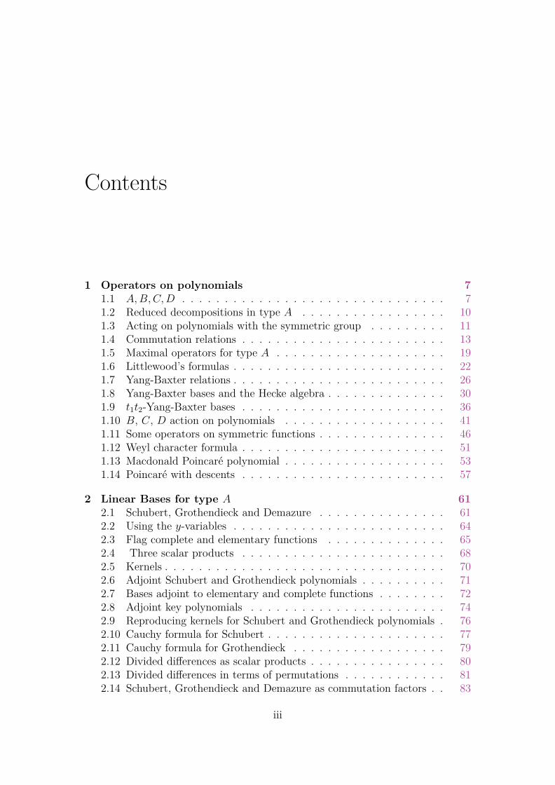
A punched v-diagram U is what results after punching holes in a v-diagram, insuch a way that there are no two holes in the same row or same column, and suchthat no two holes occupy the South-West and North-East corner of a rectangle
contained in the diagram. We forbid • • ,•
•,
•
•.
Label the rows of a v-diagram by the first entry of each row, and the columnsby v1+1, . . . , vn+n. The weight of a punched v-diagram U , that we denote xU ,is the product
∏rows xi
∏columns xj, keeping the indices of punched rows, and of
full columns. By πU we mean the reading of U columnwise, from left to right,interpreting each i as πi and ignoring the holes.
Let us give an example of a punched diagram for v = [2, 2, 4, 4, 4].
x3 x4 x7 x8 x9
6 7 8
5 6 7
2 3 4 5 6
1 2 3 4 5
x6
x5
x2
x1
coordinates and filling
x3 x8
• 7 8
5 6 7
2 • 4 5 6
1 2 3 4 •
x6
x2
x1
weight of a punched diagram
The punched 133-diagrams with two holes, together with their weights, are
• 5
3 4• 2 3x1 x4 x6
4 5• 4
• 2 3x1 x3 x6
4 •3 4
• 2 3x1 x5 x4
4 5
3 •• 2 3x1 x5 x3
• 5
3 •1 2 3x2 x4 x3
• 5
3 4
1 2 •x2 x4 x1
4 5• 4
1 2 •x2 x3 x1
.
We shall need more commutation relations.

Chapter 1 — Operators on polynomials
Lemma 1.4.2. For any positive integer n, one has
1
x1 · · ·xn+1
π1 · · · πn x1 · · ·xn =1
x1
π1 · · · πn+n∑i=1
1
xi+1
π1 · · · πi−1πi+1 · · · πn , (1.4.5)
π1 · · · πn x2 · · ·xn π1 · · · πn−1 = x3 · · ·xn+1 π1 · · · πnπ1 · · · πn−1 . (1.4.6)
Given v ∈ Nn antidominant, V its associated diagram, then
πV x1 · · ·xn =∑U
xU πU , (1.4.7)
sum over all the punched v-diagrams.
Proof. The first two assertions are obtained by iterating the relation πixi = xi+1πi+xi. Let us check the last one by recursion, adding a top row to the diagram V .
One therefore has to evaluate a product of the type πr · · · πmxU πU , where therestriction of xU to xr, . . . , xm+1 is a subword of xr · · ·xm which points out fullcolumns in U .
Let us first examine the case where xr 6∈ U . Taking specific values to simplifythe exposition, ignoring the left part figured by hearts, one has to evaluate
π15 π16 π17 π18 π19
· x16 x17 · x19
♥
♥ ♥
♥ ♥
♥ ♥
14 15 16 17 18
• 14 15 16 17
12 13 14 15 16
11 12 13 • 15
By commutation of the incomplete columns with the complete ones, one obtains
π15 π16 π17 π18 π19
· x16 x17 · x19
♥
♥ ♥
♥ ♥
♥ ♥
· 15 16 · 18
• 14 15 16 17 18
12 13 14 · 16 17
11 12 13 • 15 16
,
from which one extracts the left factor (π15π16π17 x16x17 π15π16)(π18π19 x19 π18),which, thanks to (1.4.6), is equal to x17x18x20 (π15π16π15π17π16)(π18π19π18). We

§ 1.4 — Commutation relations
therefore have transformed xU πU into xU+πU
+ , where U+ is obtained from U byadding a top row.
Let us consider now the case where xr ∈ xU . Still with the same example, onehas to evaluate
π15 π16 π17 π18 π19
x15 x16 x17 · x19
♥
♥ ♥
♥ ♥
♥ ♥
14 15 16 17 18
13 14 15 16 17
12 13 14 15 16
11 12 13 • 15
Thanks to (1.4.5), the factor π15π16π17 (x15x16x17) is equal to the sum
x16 x17 x18
π15 π16 π17+
x17 x18
x15 • π16 π17+
x16 x18
x15 π15 • π17+
x16 x17
x15 π15 π16 •.
Adding a top row to the diagram V has resulted in adding a top row to U , oradding a row with only one hole, in all possible manners such that the new holeis left of the already existing holes in the last block of columns. This finishes theproof of the lemma. QED
For example, for v = [1, 2, 2], one has
3 4
1 2 3x1x2x3 = x2x4x5
3 4
1 2 3
+ x1x4x53 4
• 2 3+ x2x3x5
• 4
1 2 3+ x1x2x5
3 4
1 • 3
+ x2x3x43 •
1 2 3+ x1x2x4
3 4
1 2 •+ x1x3x5
• 4• 2 3
+ x1x3x43 •
• 2 3+ x1x2x3
• 4
1 2 •.
Comparing the relations π1x2 = x1π1−x2 and x1(−π1) = (−π1)x2−x2, one ob-tains a symmetry between commuting any πσ with a polynomial f , and commutingfω and πωσ−1ω :
Lemma 1.4.3. Given n, σ ∈ Sn, and a polynomial f(xn), suppose known thecommutation
πσf(xn) =∑
ζgζ(xn) πζ .
Then one has
f(xωn) πωσ−1ω =∑
ζ(−1)`(σ)−`(ζ)πωζ−1ω gζ(x
ωn) . (1.4.8)

Chapter 1 — Operators on polynomials
Similarly,πσf(xn) =
∑ζgζ(xn) πζ
impliesf(xωn) πωσ−1ω =
∑ζ(−1)`(σ)−`(ζ)πωζ−1ω gζ(x
ωn) . (1.4.9)
For example, for n = 3, one has
π1π2x2 = x3π1π2 + x1π1 − x1 ,
x2π1π2 = π1π2x1 − π2x3 − x3
and
π1π2x22 = x2
3π1π2 + x3(x1+x3)π1 + x3x2 ,
x22π1π2 = π1π2x
21 − π2(x1(x1 + x3)− x1x2 .
Punched diagrams can also be used to describe the commutation of a productπV with a monomial. For an antidominant v ∈ Nk, n = vk+k, V associated to v, letus take the monomial xk+1 . . . xn. Transposing diagrams along the main diagonal,and introducing signs exchange the two cases. For example, for v = [2, 2], one has
2 31 2x1 x2
=
x3 x4
2 31 2
+
x2 x4
• 31 2
+
x3 x2
2 •1 2
+
x1 x4
2 3• 2
+
x3 x1
2 31 •
+
x2 x1
• 31 •
,
that is,
π2π3π1π2x1x2 = x3x4π2π3π1π2 + x2x4π3π1π2 + x3x2π2π1π2
+ x1x4π2π3π2 + x3x1π2π3π1 + x1x2π3π1 ,
while
π2π3π1π2x3x4 = x2x1π2π3π1π2 − x3x1π3π1π2 − x4x1π2π1π2
− x2x3π2π3π2 − x2x4π2π3π1 + x3x4π3π1
can be displayed as
2 31 2
x4
x3=x2
x1
2 31 2
− x3
x1
• 31 2
− x4
x1
2 •1 2
− x2
x3
2 3• 2
− x2
x4
2 31 •
+x3
x4
• 31 •
.
The operators of the type (1.3.1) and preserving polynomials are character-ized in [125]. They are essentially deformations of divided differences, thoughtheir explicit expression can look more frightening. For example, the operators(depending on the parameters u1, . . . , u4, p, q, r)
f → f((qu1 + pu3)xi + (qu2 + pu4))(u3xi+1 + u4)
u1u4 − u2u3
∂i + rf si := f Di
do satisfy the braid relations.

§ 1.5 — Maximal operators for type A
1.5 Maximal operators for type AThe operators associated to the maximal permutation ω = [n, . . . , 1] play aproeminent role. In fact, they all come from the projector onto the alternating1-dimensional representation of Sn, already used by Cauchy and Jacobi :
f →∑σ∈Sn
(−1)`(σ) fσ .
Indeed, writing ∆ for the Vandermonde det(xj−1i )ni,j=1 =
∏1≤i<j≤n(xi−xj), with
ρ = [n−1, . . . , 0], and thus xρ = xn−11 xn−2
2 · · ·x0n, one has the following proposition.
Proposition 1.5.1. Given x of cardinality n, the divided differences ∂ω, πω andπω verify :
∂ω =∑σ∈Sn
(−1)`(σ)σ1
∆, (1.5.1)
πω = xρ∑σ∈Sn
(−1)`(σ)σ1
∆, (1.5.2)
πω =∑σ∈Sn
(−1)`(σ)σ(xρ)ω
∆. (1.5.3)
Proof. As in the case n = 2, we prefer to characterize operators by their action ona basis. The monomials xu : u ≤ ρ are a basis of Pol(n) as a free Sym(n)-module.They all are sent to 0 by ∂ω as well as by
∑±σ∆−1 for degree reasons, except xρ
which is sent to 1 (this is the only computation to perform) by both operators.This proof can be adapted for πω and πω. QED
We have not mentioned Tω in the proposition, because this is not a sym-metrizer, since, for n = 2 for example, x2T1 = x1. However, x2(T1 + 1) = x1 + x2
and 1(T1 + 1) = t+ 1. This indicates that one has to take the Yang-Baxter defor-mation of Tω for v = [1, t, . . . , tn−1] if one wants a symmetrizer. Indeed one has,as we shall see in more details in (1.9.9), the following symmetrizer in the Heckealgebra (as shows the last expression):
(T1 + 1)
(T2 +
t− 1
t2 − 1
)(T3 +
t− 1
t3 − 1
)· · · (T1 + 1)
(T2 +
t− 1
t2 − 1
)(T1 + 1)
=∑σ∈Sn
Tσ =∏
1≤i<j≤n
(txi − xj) ∂ω .
We shall frequently use the action of ∂ω on a product f1(x1) · · · fn(xn) of func-tions of a single variable. In that case, the sum
∑σ∈Sn
(−1)`(σ)(f1(x1) · · · fn(xn)
)σis equal to the determinant
∣∣∣fi(xj)∣∣∣, and one may view
f1(x1) · · · fn(xn) ∂ω =∣∣∣fi(xj)∣∣∣
i,j=1...n∆−1 (1.5.4)
Chapter 1 — Operators on polynomials
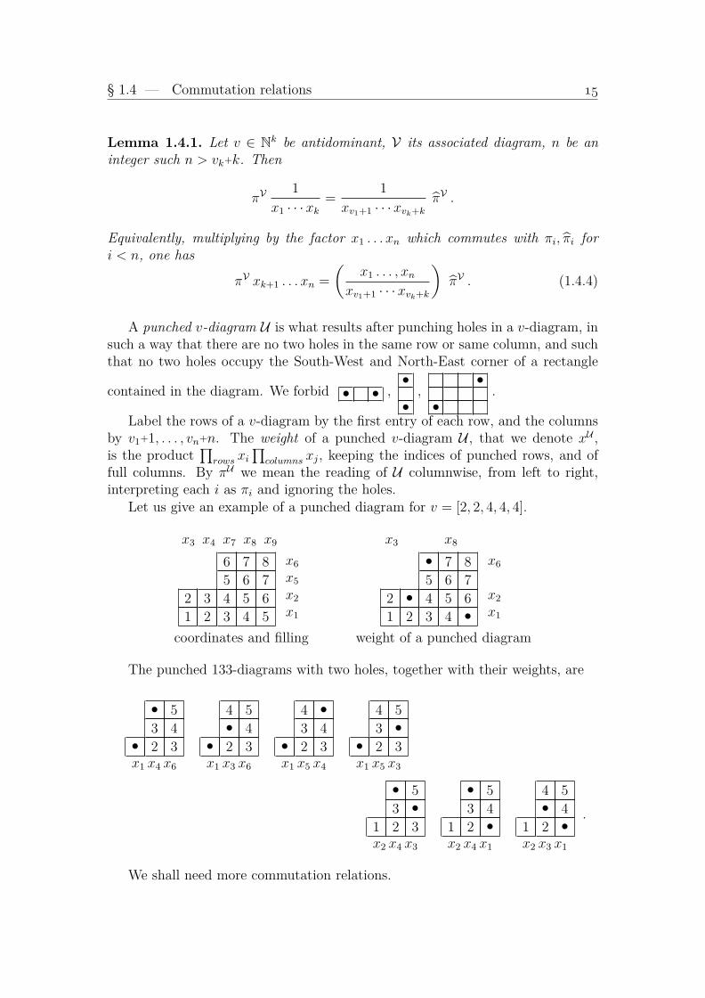
as the discrete Wronskian of the functions f1, . . . , fn. .Schur functions correspond to the case where f1, . . . , fn are powers of a variable,
factorial Schur functions arise when taking instead modified powers x(x−1) . . . (x−k), while q-factorial Schur functions stem from q-powers (x−1)(x−q) . . . (x−qk).More precisely, for any v ∈ Nn, the Schur function sv(xn) is equal to xv+ρ ∂ω, thefactorial Schur function of index v is equal to(
x1(x1−1) . . . (x1−v1−n+2)). . .(xn(xn−1) . . . (xn−vn+1)
)∂ω
and the q-factorial Schur function of index v is equal to((x1−1)(x1−q) . . . (x1−q
v1+n−1)). . .(
(xn−1)(xn−q) . . . (xn−qvn))∂ω .
For example, when n = 3 and v = [5, 2, 1], then the corresponding factorial Schurfunction is equal to
(x1 − 1) . . . (x1 − q6)(x2 − 1)(x2 − q)(x2 − q2)(x3 − 1)∂321
=1
∆
∣∣∣∣∣∣(x1−1) . . . (x1−q
6) (x2−1) . . . (x2−q6) (x3−1) . . . (x3−q
6)(x1−1) . . . (x1−q
2) (x2−1) . . . (x2−q2) (x3−1) . . . (x3−q
2)x1−1 x2−1 x3−1
∣∣∣∣∣∣ .We shall interpret it later as the specialization y1 = 1, y2 = q, y3 = q2, . . . of theGraßmannian Schubert polynomial Y125(x,y).
§ 1.5 — Maximal operators for type A
Divided differences can be defined for any pair xi, xj, and not only consecutivevariables :
∂i,j : f → (f − f τij)(xi − xj)−1 ,
τij being the transposition of xi, xj. We shall need these differences to factorize∂ω.
Lemma 1.5.2. Let n = 2m, ω′ = [m, . . . , 1, 2m, . . . ,m+1], ω = [2m, . . . , 1]. Then
∂ω′ ∂1,m+1∂2,m+2 . . . ∂m,2m ∂ω′ = (−1)(m2 )m! ∂ω . (1.5.5)
Proof. The left-hand side commutes with multiplication by elements of Sym(xn),and decreases degree by
(m2
). It is therefore sufficient to test its action on xρ to
characterize it. One has xρ∂ω′ = xmm,0m , xρ∂ω′ ∂1,m+1 . . . ∂m,2m =
∑xv, sum over
all v ∈ Nn such that vi + vm+i = m−1, i = 1, . . . ,m. Each such monomial has anon-zero image under ∂ω′ if and only if v1, . . . , vm is a permutation of [m−1, . . . , 0].There are m! such monomials, which each contribute to xm−1,...,0,0,...,m−1∂ω′ =
(−1)(m2 ) to the right-hand side. QED
For example, for n = 4, one has ∂2143∂13∂24∂2143 = −2∂4321. Many otherdecompositions are possible, e.g.
∂12∂14∂34∂23∂13∂24 = ∂4321 = ∂14∂13∂24∂23∂24∂13 = ∂23∂13∂24∂14∂34∂12 .

Chapter 1 — Operators on polynomials
1.6 Littlewood’s formulasOne can combine the above operators with change of variables xi → ϕ(xi). Themaximal divided difference ∂ω becomes
∑(±σ) ∆(ϕ(x))−1 = ∂ω∆(x)∆(ϕ(x))−1,
and it remains to find functions ϕ furnishing an interesting Vandermonde ∆(ϕ(x)).Notice that if ϕ(xi) = g(xi)/f(xi), then∣∣∣f(xi)
n−1 f(xi)n−2g(xi) · · · g(xi)
n−1∣∣∣i=1..n
=∏i
(f(xi)n−1 ∆(ϕ(x)) .
Taking f(xi) = xi, g(xi) = 1 + xki , k ≥ 0, and remarking that (1 + xki )/xi − (1 +xkj )/xj = (x−1
i − x−1j )(1− xixjsk−2(xi+xj)
), one obtains that
∣∣∣xn−1i xn−2
i (1+xki ) · · · (1+xki )n−1∣∣∣i=1...n
∆(x)−1
= (1 + xk2)(1 + xk3)2 . . . (1 + xn)n−1 πω
=∏
1≤i<j≤n
(1− xixjsk−2(xi+xj)
), (1.6.1)
the first equality resulting from the definition of πω.In the case k = 2, the preceding determinant can be transformed into∣∣∣xn−1
i xn−2i (1+x2
i ) xn−2i (1+x4
i ) · · · (1+x2n−2i )
∣∣∣i=1...n
.
Since the operator πω sends xv, v ∈ Nn onto the Schur function sv(x), thepreceding identity, still in the case k = 2, can be written as∏
1≤i<j≤n
(1− xixj) = (1 + x2
2)(1 + x23)2 . . . (1 + x2
n)n−1) πω
= (1 + x22)(1 + x4
3) . . . (1 + x2n−2n ) πω
=∑
ε=[ε1,...,εn]∈0,1n(−1)|ε|s[0ε1,2ε2,...,(2n−2)εn](x) = 1 + s02(x) + s004(x) + s024(x) + . . .
= 1− s11(x) + s211(x)− s222(x) + . . .
= 1 +∑r,α
(−1)|α|s(α|α+1r)(x) , (1.6.2)
sum over all r, all α = [α1, . . . , αr], α1 > α2 > . . . αr ≥ 0, using the Frobeniusnotation6 for partitions.
Similar identities, known to Littlewood [143], [146, p. 78], can be obtained aseasily, the reordering of the indices of the Schur functions being translated into
6

§ 1.6 — Littlewood’s formulas
properties of diagonal hooks.∏i
(1− xi)∏
1≤i<j≤n
(1− xixj) = (1− x1)(1− x3
2) . . . (1− x2n−1n ) πω
=∑
ε=[ε1,...,εn]∈0,1n(−1)|ε|s[ε1,3ε2,...,(2n−1)εn](x)
= 1− s1(x)− s03(x) + s13(x)− s005(x) + s105(x) + s035(x)− s135(x) + . . .
= 1− s1(x) + s21(x)− s22(x)− s311(x) + s321(x)− s332(x) + s333(x) + . . .
= 1 +∑α
(−1)|α|s(α|α)(x) . (1.6.3)
∏1≤i≤j≤n
(1− xixj) = (1− x2
1)(1− x42) . . . (1− x2n
n ) πω
=∑
ε=[ε1,...,εn]∈0,1n(−1)|ε|s[2ε1,4ε2,...,2nεn](x)
= 1− s2(x)− s04(x) + s24(x)− s006(x) + s206(x) + s046(x)− s246(x) + . . .
= 1− s2(x) + s31(x)− s33(x)− s411(x) + s431(x)− s442(x) + s444(x) + . . .
= 1 +∑r,β
(−1)|β|s(β+1r|β)(x) . (1.6.4)
n∏i=1
(1− xi)∏
1≤i≤j≤n
(1− xixj)
= (1− x1)(1− x21)(1− x2
2)(1− x32) . . . (1− xnn)(1− xn+1
n ) πω
=(1− s1(x) + s11(x)− s111(x) + . . .
) ∑εi∈0,1
(−1)|ε|s[2ε1,4ε2,...,2nεn](x) . (1.6.5)
One can generalize these formulas by adding letters to the alphabet x. Forexample, using x ∪ 1 in (1.6.2), one obtains∣∣∣∣∣∣∣∣∣xn1 xn−1
1 + xn+11 . . . 1 + x2n
1... ... ...xnn xn−1
n + xn+1n . . . 1 + x2n
n
1 1 . . . 1
∣∣∣∣∣∣∣∣∣1
∆(x)=
n∏i=1
(1− xi)2∏
1≤i<j≤n
(xixj − 1) , (1.6.6)
the factor∏
(1−xi)2 being due to s11(x + 1) = s11(x) + s1(x) and ∆(x+1) =
∆(x)∏
(1−xi). More variations of this type can be found in [105].All the preceding formulas can be interpreted, in terms of λ-rings, as describing
the plethysms Λi(S2) or Λi(Λ2), and have counterparts describing Si(S2) or Si(Λ2).Let us show that the symmetrizer πω still allow to describe the generating functionof this last plethysms.
Chapter 1 — Operators on polynomials
Proposition 1.6.1. For a given n, one has∏i≤j
(1− xixj)−1 =1
(1−x21)(1−x2
1x22) . . . (1−x2
1 . . . x2n)πω (1.6.7)
=∑
even rows
sλ(x)
∏i<j
(1− xixj)−1 =1
(1−x1x2)(1−x1 . . . x4)(1−x1 . . . x6) . . .πω(1.6.8)
=∑
even columns
sλ(x)
∏(1−xi)
−1∏i<j
(1− xixj)−1 =1
(1−x1)(1−x1x2) . . . (1−x1 . . . xn)πω (1.6.9)
=∑
sλ(x)∏(1−xi)
−2∏i<j
(1− xixj)−1 =1
(1−x1)2(1−x1x2)2 . . . (1−x1 . . . xn)2πω(1.6.10)
=∑
(λ1−λ2+1)(λ2−λ3+1) . . .(λn+1)sλ(x).(1.6.11)
Proof. One can use induction on n, factorizing πω = πω′πω, with ω′ = [n−1, . . . , 1].Thus one is left with computing the image under πω of the quotient of the twosuccessive denominators appearing in the left-hand sides. For the first formula, itmeans computing
(1− x1xn) . . . (1− x1xn−1)(1− x2n)(1− x1 . . . xn)−1πω
= (1− xne1 + · · ·+ (−xn)nen))(1− x1 . . . xn)−1πω ,
e1, . . . , en being the elementary symmetric functions in xn, and therefore com-muting with πω. Since xn, . . . , xn−1
n are sent to 0, and (−xn)nπω = −x1 . . . xn, theabove expression is equal to 1, thus proving (1.6.7). The other formulas require nomore pain. Moreover, the rational functions in the right-hand sides expanding assums of dominant monomials, the expressions in terms of Schur functions followimmediately. QED
One should try expressions more general than products of factors (1 ± u)±1,with u monomial. I shall give a single example.
Lemma 1.6.2. Given n, then
1
(1−x1−x2)(1−x22)(1−x111−x222)(1−x2222) . . .πω
=∏i
1
1− xi − x2i
∏i<j
1
1− xixj. (1.6.12)
§ 1.6 — Littlewood’s formulas
Proof. Let Gn be the right-hand side. Using induction on n, one has to computeGn−1/Gnπω. This depends on parity, and taking n = 4, 5 will be generic enoughto follow the proof.
G3/G4π4321 = (1−x1x4)(1−x2x4)(1−x3x4)(1− x4 − x24) π4321
=4∏i=1
(1− xix4)π4321 − x4(1−x1x4)(1−x2x4)(1−x3x4)π4321 .
One has already seen that∏
(1 − xix4)π4321 = 1 − x2222, and one checks thatall the monomials appearing in x4(. . . ) are sent to 0 under π4321. In the case ofG4/G5π54321 on the contrary, the monomial −x11003 is such that −x11003π54321 =−x11111, and thus, G4/G5π54321 = 1 − x22222 − x11111. In both cases, the resultingfactor is what is required by the left-hand side of (1.6.12) to ensure equality. QED
The left-hand side of (1.6.12) expands as a positive sum of Schur functions,which multiplicities that are easily written in terms of the multiplicities of partsin the conjugate partitions.
Chapter 1 — Operators on polynomials
1.7 Yang-Baxter relations
With a little more work, one can construct operators offering still more parameters.The uniform shift Di → Di + 1, i = 1, . . . , n−1, destroys in general the braid
relations7. For example,
(1 + s1)(1 + s2)(1 + s1) = 2 + 2s1 + s2 + s1s2 + s2s1 + s1s2s1
6= (1 + s2)(1 + s1)(1 + s2) .
However
(1 + s1)(1
2+ s2)(1 + s1) = (1 + s2)(
1
2+ s1)(1 + s2) ,
because both sides expand (in the group algebra of S3) into the sum of all per-mutations.
Therefore, one abandons uniform shifts, but how to find compatible shifts like1, 1/2, 1 ?
The solution is due to Young [195], and called Yang-Baxter equation [194, 5]because Young-Yang-Baxter would be confusing.
One chooses an arbitrary vector of parameters v = [v1, . . . , vn] (called spec-tral vector), and each time one operates with Di, i = 1, . . . , n−1, one modifiesaccordingly the spectral vector by v → vsi.
Now, the shift to use depends only on the difference of the spectral valuesexchanged, with similar rules for the different varieties of operators Di.
More precisely, given i, let a = vi, b = vi+1 the corresponding components ofthe spectral vector. Then, instead of si, ∂i, πi, πi, Ti respectively, one takes
si +1
b− a, ∂i +
1
b− a, πi +
1
b/a− 1, πi +
1
b/a− 1, Ti +
t− 1
b/a− 1
(the careful reader adds “provided b 6= a”).For n = 3, the Yang-Baxter relations for si, ∂i, πi and Ti, and a spectral vector
v are, writing v2−v1 = a, v3−v2 = b, v2/v1 = α, v3/v2 = β,
7it only works for πi → πi + 1 = πi.

§ 1.7 — Yang-Baxter relations
123
213 132
231 312
321
s1 + 1a
s2 + 1b
s2+ 1a+b
s1+ 1a+b
s1 + 1b
s2 + 1a
123
213 132
231 312
321
∂1 + 1a
∂2 + 1b
∂2+ 1a+b
∂1+ 1a+b
∂1 + 1b
∂2 + 1a
123
213 132
231 312
321
π1 + 1α−1
π2 + 1β−1
π2+ 1αβ−1
π1+ 1αβ−1
π1 + 1β−1 π2 + 1
α−1
123
213 132
231 312
321
T1 + t−1α−1
T2 + t−1β−1
T2+ t−1αβ−1
T1+ t1−1αβ−1
T1 + t−1β−1 T2 + t−1
α−1
The fact that each hexagon closes means that the two paths from top to bottomgive equal elements when evaluated as products of the labels on the edges.
Thanks to the Yang-Baxter relations, to each spectral vector v, is associateda family of operators Dv
σ : σ ∈ Sn, obtained by taking products corresponding toreduced decompositions.
Chapter 1 — Operators on polynomials
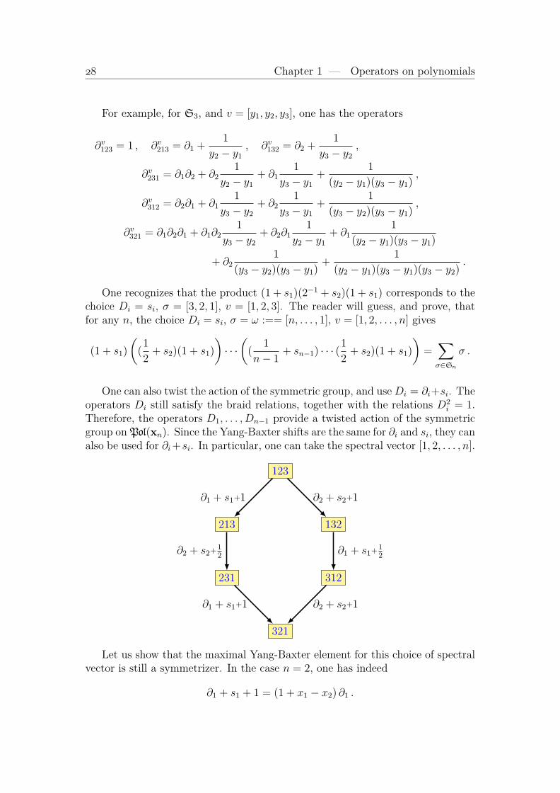
For example, for S3, and v = [y1, y2, y3], one has the operators
∂v123 = 1 , ∂v213 = ∂1 +1
y2 − y1
, ∂v132 = ∂2 +1
y3 − y2
,
∂v231 = ∂1∂2 + ∂21
y2 − y1
+ ∂11
y3 − y1
+1
(y2 − y1)(y3 − y1),
∂v312 = ∂2∂1 + ∂11
y3 − y2
+ ∂21
y3 − y1
+1
(y3 − y2)(y3 − y1),
∂v321 = ∂1∂2∂1 + ∂1∂21
y3 − y2
+ ∂2∂11
y2 − y1
+ ∂11
(y2 − y1)(y3 − y1)
+ ∂21
(y3 − y2)(y3 − y1)+
1
(y2 − y1)(y3 − y1)(y3 − y2).
One recognizes that the product (1 + s1)(2−1 + s2)(1 + s1) corresponds to thechoice Di = si, σ = [3, 2, 1], v = [1, 2, 3]. The reader will guess, and prove, thatfor any n, the choice Di = si, σ = ω :== [n, . . . , 1], v = [1, 2, . . . , n] gives
(1 + s1)
((1
2+ s2)(1 + s1)
)· · ·(
(1
n− 1+ sn−1) · · · (1
2+ s2)(1 + s1)
)=∑σ∈Sn
σ .
One can also twist the action of the symmetric group, and useDi = ∂i+si. Theoperators Di still satisfy the braid relations, together with the relations D2
i = 1.Therefore, the operators D1, . . . , Dn−1 provide a twisted action of the symmetricgroup on Pol(xn). Since the Yang-Baxter shifts are the same for ∂i and si, they canalso be used for ∂i+si. In particular, one can take the spectral vector [1, 2, . . . , n].
123
213 132
231 312
321
∂1 + s1+1 ∂2 + s2+1
∂2 + s2+ 12
∂1 + s1+ 12
∂1 + s1+1 ∂2 + s2+1
Let us show that the maximal Yang-Baxter element for this choice of spectralvector is still a symmetrizer. In the case n = 2, one has indeed
∂1 + s1 + 1 = (1 + x1 − x2) ∂1 .

§ 1.7 — Yang-Baxter relations
Lemma 1.7.1. Given n, let
ω =
((D1+1) . . . (Dn−1 +
1
n− 1)
)((D1+1) . . . (Dn−2 +
1
n− 2)
). . .(D1
).
Thenω =
∏1≤i<j≤n
(1 + xi − xj) ∂ω . (1.7.1)
Proof. Both sides of (1.7.1) commute with multiplication with symmetric func-tions, it is therefore sufficient to test their action on a basis of Pol(xn) as a freeSym(xn) module. But instead of the basis of monomials xv : v ≤ ρ used above,we shall use a basis of homogeneous polynomials Yv : v ≤ ρ in their linearspan, such that each Yv has a least one symmetry8 in some xi, xi+1, except forYn−1,...,0 = xρ. But using symmetric rational functions in xn instead of elements ofSym(xn), we can take the polynomials Yv
∏1≤i<j≤n(1+xj−xi) as a test cohort. All
these elements, except in the case v = ρ, are sent to 0 by∏
1≤i<j≤n(1 +xi−xj) ∂ωbecause the factor
∏i 6=j(1 + xi − xj), being symmetrical, commutes with ∂ω, and
because Yv∂ω = 0 for degree reasons.On the other hand, if Yv has the symmetry xi, xi+1, then, by commutation,
Yv∏
1≤i<j≤n
(1+xj−xi)(∂i + si + 1) = Yv
( ∏1≤i<j≤n
(1+xj−xi)
)(1+xi−xi+1) ∂i
= Yv∂i
( ∏1≤i<j≤n
(1+xj−xi)
)(1+xi−xi+1) = 0 .
Since, thanks to Yang-Baxter equation, one can factorize on the left of ω anyDi + 1, the image of Yv
∏(1 + xj − xi) under ω is 0 when v 6= ρ. Thus, both
sides of (1.7.1) coincide up to multiplication by a rational symmetric function. Todetermine this constant, it is sufficient to see that
1(∂1+s1+1)(∂1+s1+2−1) · · · = n! =∏
1≤i<j≤n
(1+xi−xj) ∂ω ,
and this ensures the required equality. QEDThe Yang-Baxter rules do not exhaust the realm of interesting factorized ex-
pressions. Let us take9
((1− y1∂1)(1− y1∂2) · · · (1− y1∂n−1))
((1− y2∂1)(1− y2∂2) · · · (1− y2∂n−2)) · · · ((1− yn−1∂1))
8tTo show that such a basis exists is easy by induction on n, we shall see later that theSchubert polynomials Yv(x,0) satisfy such properties.
9This product of divided differences is the generating function of Schubert polynomials in thepair of alphabets y,0, in the algebra of divided differences, also called the Nil-Coxeter algebra[39] see (8.3.2).

Chapter 1 — Operators on polynomials
and show that this element can be used to transform the staircase monomial xρ,with ρ = [n−1, . . . , 0], into a product of factors of the type xi − yj.
Let us make the step-by-step computation for n = 4, displaying the factors ofthe polynomials planarly.
x3
x2 x2
x1 x1 x1
1−y1∂1−−−→
x3
x2 x2
x1 x1 x1−y1
1−y1∂2−−−→
x3
x2 x2−y1
x1 x1 x1−y1
1−y1∂3−−−→
x3−y1
x2 x2−y1
x1 x1 x1−y1
· · · 1−y3∂1−−−→
x3−y1
x2−y2 x2−y1
x1−y3 x1−y2 x1−y1
.
Each step is of the type f xi(1 − y∂i) = f (xi − y), with f symmetrical inxi, xi+1. In final, we have obtained the function
∏i+j≤4(xi − yj) by using only
that 1∂i = 0, xi∂i = 1. This function, together with the “staircase monomial”x3210, will play a key role in all the sequel. This identity can be written morecompactly, still reading the planar arrays by columns (reading by rows still worksin the present case), as
x3
x2 x2
x1 x1 x1
1−y1∂1 1−y1∂2 1−y1∂3
1−y2∂1 1−y2∂2
1−y3∂1
=
x3−y1
x2−y2 x2−y1
x1−y3 x1−y2 x1−y1
. (1.7.2)
1.8 Yang-Baxter bases and the Hecke algebraThe Yang-Baxter relations constitute a powerful tool to define linear bases withan explicit action of the Hecke algebra (or of the different algebras obtained byspecialization, the first interesting one being the group algebra of the Weyl group).
In this section we shall change the conventions for the Hecke algebra, comparedto the preceding section, to bring into prominence some symmetries.
The Hecke algebra Hn of the symmetric group Sn is the algebra generated byT1, . . . , Tn−1 satisfying the braid relations together with the Hecke relations
(Ti − t1)(Ti − t2) = 0 , i = 1, . . . , n−1 ,
for some fixed generic parameters t1, t2. For Macdonald polynomials, one takest1 = t, t2 = −1. The 0-Hecke algebra is the specialisation t1 = 0, t2 = −1 of

§ 1.8 — Yang-Baxter bases and the Hecke algebra
the Hecke algebra (that one can realize as the algebra generated by π1, . . . , πn−1).The 00-Hecke algebra, also called NilCoxeter algebra, is the specialisation t1 = 0,t2 = 0. It can be realized as the algebra generated by ∂1, . . . , ∂n−1. .
From the point of view of operators, the Hecke algebra is the algebra gen-erated by operators Ti such that each Ti acts on xi, xi+1 only, commutes withSym(xi, xi+1), and acts on 1, xi+1 by
1Ti = t1 & xi+1 Ti = −t2xi .
One has therefore Ti = πi(t1 + t2)− sit2.The general Yang-Baxter equation10 depends on two generic parameters α, β :(T1 +
t1+t2α−1
)(T2 +
t1+t2αβ−1
)(T1 +
t1+t2β−1
)=
(T2 +
t1+t2β−1
)(T1 +
t1+t2αβ−1
)(T2 +
t1+t2α−1
). (1.8.1)
Graphically, it reads
123
213 132
231 312
321
T1 + t1+t2α−1
T2 + t1+t2β−1
T2+ t1+t2αβ−1
T1+ t1+t2αβ−1
T1 + t1+t2β T2 + t1+t2
α
Given n, one takes an arbitrary spectral vector [γ1, . . . , γn] of indeterminates.The Yang-Baxter basis fγ
σ : σ ∈ Sn corresponding to [γ1, . . . , γn] is definedrecursively, as follows, starting from fγ
σ = 1 for the identity permutation:
fγσsi
= fγσ
(Ti +
t1 + t2γσi+1
/γσi − 1
)for σi < σi+1 . (1.8.2)
The consistency of the definition is insured by the Yang-Baxter equation (1.8.1).Notice that arrows are reversible in the generic case. Indeed, for any i, any
10The Yang-Baxter relations for the group algebra of Sn, for the algebra of divided differences,and for the algebra of isobaric divided differences are the limits t1 = 1, t2 = −1, t1 = 0, t2 = 0,t1 = 1, t2 = 0 of (1.8.1 respectively.

Chapter 1 — Operators on polynomials
γ 6= 0, 1, one has(Ti+
t1+t2γ−1
)(Ti+
t1+t2γ−1−1
)=
(t1+
t1+t2γ−1
)(t1+
t1+t2γ−1−1
)= −
(t1γ+t2)(t1+t2γ)
(γ − 1)2.
It is clear that the set fγσ : σ ∈ Sn constitute a linear basis of Hn, be-
cause fσ = Tσ +∑
v:`(v)<`(σ) cvσTv. Since this basis is generated using the Ti’s,
it is immediate to write the matrices representing the Hecke algebra in this ba-sis. The matrices representing each Ti are made of 2 × 2 blocks correspondingto the spaces 〈fγ
σ,fγσsi〉. They generalize the semi-normal representation of the
symmetric group due to Young11.Indeed, for S2, and the spectral vector [1, γ], the Yang-Baxter basis is 1, T1 +
(t1+t2)(γ−1)−1, and the matrix representing T1 is given on the left, while Young’smatrix (which is the limit for γ = (−t1/t2)g, (−t1/t2) → 1) is given on the right[163] :[
−(t1+t2)(γ−1)−1 −(t1γ+t2)(t1+γt2)(γ−1)−2
1 (t1+t2)(γ−1−1)−1
],
[−g−1 1− g−2
1 g−1
](1.8.3)
One could write the similar matrices for the other types B,C,D, once theYang-Baxter relations have been written for these types.
Irreducible representations can be obtained by either degeneration of the spec-tral vector, or by making the Hecke algebra act on polynomials. For example, inthe case of the symmetric group, a Specht representation is obtained by actingon a product of Vandermondes on consecutive variables. Similarly, acting on aproduct of t-t Vandermondes
∏a≤i<j≤b(xi−txj) on blocks of consecutive variables
produces an irreducible representation of the Hecke algebra.Yang-Baxter bases possess many symmetries. Let f → ω ? f ? ω be the auto-
morphism of Hn induced by Tσ → ω ? Tσ ? ω = Tωσω. Then one hasLemma 1.8.1. The Yang-Baxter bases associated to the spectral vectors [y1, . . . , yn]and [y−1
n , . . . , y−11 ] satisfy the relations
fy−1n ,...,y−1
1σ = ω ? fy1,...,yn
ωσω ? ω , σ ∈ Sn . (1.8.4)
Proof. In the case n = 2, this is the identity
T1 +t1 + t2
y−11 /y−1
2 − 1= ω ?
(T1 +
t1 + t2y2/y1 − 1
)? ω = T1 +
t1 + t2y2/y1 − 1
.
For a general σ and i such that `(σsi) ≥ `(σ), putting γ = y−1n−i/y
−1n+1−i, one has
fy−1n ,...,y−1
1σ
(Ti +
t1 + t2γ − 1
)= (ω ? fy1,...,yn
ωσω ? ω)
(ω ?
(Ti +
t1 + t2γ − 1
)? ω
)= ω ?
(fy1,...,ynωσω
(Ti +
t1 + t2yn+1−i/yn−i − 1
))? ω ,
11We have taken generic parameters. To build general representations, one also needs blocksof size 1!.

§ 1.8 — Yang-Baxter bases and the Hecke algebra
and this proves the statement by induction on length. QEDWe also need another involution f → f induced by
Ti → Ti = Ti − (t1+t2) , t1 → −t2 , t2 → −t1 .
Notice that T1, . . . , Tn−1 satisfy the braid relations, together with the Hecke rela-tions (
Ti + t2
)(Ti + t1
)= 0 ,
and that TiTi = −t1t2.Let now f → f∨ be the anti-automorphism induced by (Tσ)∨ = Tσ−1 . Define
a quadratic form ( , )H on Hn by
(f , g)H = f g∨ ∩ Tω , (1.8.5)
i.e. by taking the coefficient of Tω in the product f g∨.The basis Tσ is clearly the adjoint of Tωσ, i.e. one has(
Tωσ , Tζ
)H= δσ,ζ , σ, ζ ∈ Sn .
Testing the statements on the pairs Tσ, Tζ , one checks :
(Ti f , g)H = (f , Tn−ig)H & (fTi , g)H = (f , gTi)H . (1.8.6)
The quadratic form can be restricted to two-dimensional spaces, for which onehas the following property of a Yang-Baxter basis.
Lemma 1.8.2. Let f, g ∈ Hn, i, γ be such that(f , g
)H= 0 &
(f(Ti +
t1 + t2γ − 1
) , g
)H= 1 .
Then(f , g(Ti +
t1 + t2γ−1 − 1
)
)H= 1 &
(f(Ti +
t1 + t2γ − 1
) , g(Ti +t1 + t2γ−1 − 1
)
)H= 0 .
Proof.One transfers the factor (Ti+•) to the left, and uses that (Ti+(t1+t2)(γ−1)−1)(Ti+(t1+t2)(γ−1−1)−1) be a scalar. QED
In other words, the two Yang-Baxter bases associated with the spectral vectors[1, γ] and [1, γ−1] are adjoint of each other with respect to ( , )H.
Combining the Yang-Baxter relations and the preceding lemma, one can eval-uate scalar products of factorized elements. For example(
(T1 +t1+t2α−1
)(T2 +t1+t2αβ−1
)(T1 +t1+t2β−1
) , (T1 +t1+t21α−1
)(T2 +t1+t21αβ−1
)
)H
=
((T1 +
t1+t2α−1
)(T2 +t1+t2αβ−1
)(T1 +t1+t2β−1
)(T2 +t1+t21αβ−1
)(T1 +t1+t21α−1
)
)∩ T321

Chapter 1 — Operators on polynomials
can be computed by reducing the length of the expression, replacing some factorsTi + (t1+t2)(γ−1−1)−1) by a sum of two terms (Ti+c1) + c2 to fit the parametersin the Yang-Baxter relations. But it is simpler to move the RHS of the scalarproduct to the left, obtaining(
(T2 +t1+t21αβ−1
)(T1 +t1+t21α−1
)(T1 +t1+t2α−1
)(T2 +t1+t2αβ−1
)(T1 +t1+t2β−1
) , 1
)H
which reduces to a scalar multiple of (T1 + (t1+t2)(β−1)−1, , 1)H
= 0.This example is some instance of a general orthogonality of Yang-Baxter bases.
Let us write Ti(a, b) = Ti + (t1+t2)(yby−1a − 1)−1, yω = [yn . . . , y1], and first settle
the case of the maximal Yang-Baxter element.
Lemma 1.8.3. The element fyω satisfies the n! equations(fyω , fyω
σ
)H= δ1,σ . (1.8.7)
Proof. One takes a reduced decomposition si1si2 . . . sir of σ. Then there existsintegers such that
fyωσ = Ti1(a1, b1)Ti2(a2, b2) . . . Tir(ar, br) .
One can factor ω = σ−1(σω), and correspondingly write the maximal element as
fyω = Tn−i1(b1, a1)Tn−i2(b2, a2) . . . Tn−ir(br, ar) • • • .
Tanks to (1.8.6) ,
(fyω , Ti1(a1, b1) . . . Tir(ar, br)
)H=(Tn−ir(ar, br) . . . Tn−i1(a1, b1)Tn−i1(b1, a1) . . . Tn−ir(br, ar) • •• , 1
)His a scalar multiple of
(• • • , 1
)H, and therefore null if σ is not the identity
permutation. QEDThe following duality property of Yang-Baxter bases is given in [114, Th.5.1].
Theorem 1.8.4. The Yang-Baxter bases associated to the spectral vectors [y1, . . . , yn]and [yn, . . . , y1] satisfy the relations(
fyσ , fyω
ζ
)H= δσ,ωζ , (1.8.8)
that is, they are adjoint of each other.

§ 1.8 — Yang-Baxter bases and the Hecke algebra
Proof. When σ = ω, this is property (1.8.7). One proves the general statement bydecreasing induction on `(σ), using Lemma 1.8.2. QED
Given any product(Ti + α(t1+t2)
). . .(Tk + γ(t1+t2)
)=∑ζ
cζTζ ,
then the product (Ti − α(t1+t2)
). . .(Tk − γ(t1+t2)
)is equal to
∑ζ cζ Tζ . This remark allows to rewrite the orthogonality relation
(1.9.5). Define the coefficients cησ by fyσ =
∑cησ(y)Tη, and recall that the involu-
tion c→ c acts by t1 → −t2, t2 → −t1.
Corollary 1.8.5. Let σ, ζ ∈ Sn. Then∑η∈Sn
cησ(y−1n , . . . , y−1
1 ) cωηζ (y) = δωσ,ζ (1.8.9)∑η∈Sn
cησ(y) cηωζ (y) = δσ,ζω (1.8.10)
Proof. One uses thatfyωζ =
∑η
cηζ(y−1n , . . . , y−1
1 ) Tη ,
and that the symmetry (1.8.4) translates into cησ(y−1n , . . . , y−1
1 ) = cωηωωσω(y1, . . . , yn).QED
Each of the relations (1.8.9) or (1.8.10) can be used to describe the inverse ofthe matrix of Yang-Baxter coefficients
[cησ].

Chapter 1 — Operators on polynomials
1.9 t1t2-Yang-Baxter bases
For k > 1, write
[k] = tk−11 − t2tk−2
1 + · · ·+ (−t2)k−1 , [−k] = tk−12 − t1tk−2
2 + · · ·+ (−t1)k−1 ,
with the convention that [0] = 0, [1] = 1 = [−1]. Define, for all k ∈ Z, k 6= 0,
Ti(k) = Ti +t1 + t2
(−t1/t2)k − 1=
Ti − tk2 [−k]−1 , k > 0
Ti − t−k1 [k]−1 , k < 0, (1.9.1)
adding Ti(0) = Ti.Thus
Ti(1) = Ti−t2, Ti(2) = Ti −t22
t2 − t1, Ti(3) = Ti −
t32t22 − t1t2 + t21
, . . . ,
Ti(−1) = Ti−t1, Ti(−2) = Ti −t21
t1 − t2, Ti(−3) = Ti −
t31t21 − t1t2 + t22
, . . .
We denote di = Ti(1) and ∇i = Ti(−1) the two factors of the Hecke relation forTi. Acting on 1, xi, one checks that
∇i = ∂i(t2xi + t1xi+1) & di = (t1xi + t2xi+1)∂i . (1.9.2)
Notice that for k > 0 one has
Ti(k)Ti(−k) = −t1t2[k−1] [k+1]
[k]2, (1.9.3)
so that, for k 6= ±1, Ti(k) and Ti(−k) are inverse of each other up to a scalar.More generally, the Yang-Baxter equation (1.8.1) implies that, for any i > 0, anyk, r ∈ Z such that k, r, k+r 6= 0, one has
Ti(k)Ti+1(k+r)Ti(r) = Ti+1(r)Ti(k+r)Ti+1(k) (1.9.4)
Taking the spectral vectors [tn−11 , −tn−2
1 t2, . . . , (−t2)n−1], and [tn−12 , −t1t
n−22 , . . . , (−t1)n−1],
one obtains a pair of adjoint Yang-Baxter bases which are exchanged by the in-volution exchanging t1, t2. We shall denote these two bases ∇σ : σ ∈ Sn anddσ : σ ∈ Sn respectively. Here is the basis associated to the spectral vector
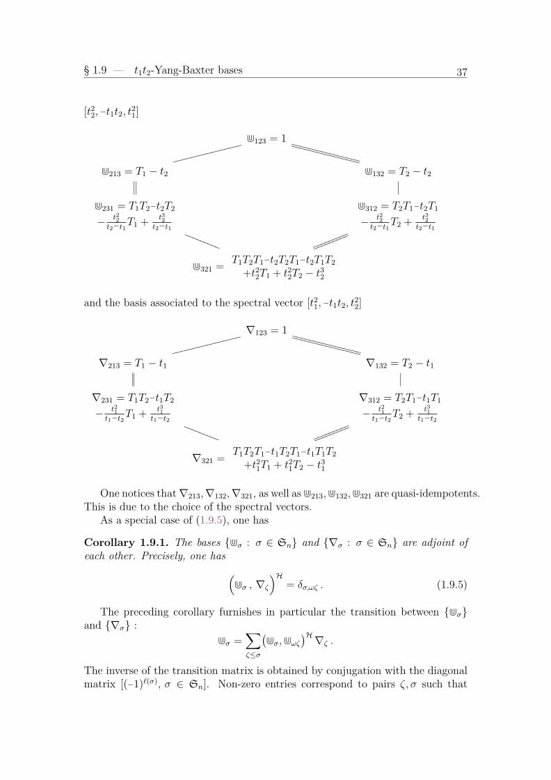
§ 1.9 — t1t2-Yang-Baxter bases
[t22, −t1t2, t21]
d123 = 1
gggggggggggggggg
WWWWWWWWWWWWWWWW
WWWWWWWWWWWWWWWW
d213 = T1 − t2 d132 = T2 − t2
d231 = T1T2−t2T2
− t22t2−t1T1 +
t32t2−t1
RRRRRRRRR
d312 = T2T1−t2T1
− t22t2−t1T2 +
t32t2−t1
llllllllllllllllll
d321 =T1T2T1−t2T2T1−t2T1T2
+t22T1 + t22T2 − t32
and the basis associated to the spectral vector [t21, −t1t2, t22]
∇123 = 1
gggggggggggggggg
WWWWWWWWWWWWWWWW
WWWWWWWWWWWWWWWW
∇213 = T1 − t1 ∇132 = T2 − t1
∇231 = T1T2−t1T2
− t21t1−t2T1 +
t31t1−t2
SSSSSSSSS
∇312 = T2T1−t1T1
− t21t1−t2T2 +
t31t1−t2
kkkkkkkkkkkkkkkkkk
∇321 =T1T2T1−t1T2T1−t1T1T2
+t21T1 + t21T2 − t31
One notices that∇213,∇132,∇321, as well as d213,d132,d321 are quasi-idempotents.This is due to the choice of the spectral vectors.
As a special case of (1.9.5), one has
Corollary 1.9.1. The bases dσ : σ ∈ Sn and ∇σ : σ ∈ Sn are adjoint ofeach other. Precisely, one has (
dσ , ∇ζ
)H= δσ,ωζ . (1.9.5)
The preceding corollary furnishes in particular the transition between dσand ∇σ :
dσ =∑ζ≤σ
(dσ,dωζ
)H∇ζ .
The inverse of the transition matrix is obtained by conjugation with the diagonalmatrix [(−1)`(σ), σ ∈ Sn]. Non-zero entries correspond to pairs ζ, σ such that

Chapter 1 — Operators on polynomials
ζ ≤ σ with respect to the Ehresmann-Bruhat order. Thus this matrix may beconsidered as “weighing” the order. We shall see later another weight given bythe Kazhdan-Lusztig polynomials.
The case where σ is a Coxeter element is specially interesting since then theinterval [1, σ] is boolean. Let us just describe the expansion of dσ when σ =[2, . . . , n, 1].
Define a function ϕ on permutations as follows, starting from ϕ([1]) = 1. Forσ ∈ Sn, if σn 6= n, then ϕ(σ) = ϕ(σ \ n)), else
ϕ(σ) = ϕ(σ \ n)[1] [2n−σn−1−1]
[n−1] [n−σn−1].
For example, ϕ([1, 3, 4, 2, 5]) = ϕ([1, 3, 4, 2]) [1][10−2−1][4][5−2]
= ϕ([1, 3, 2]) [1][7][4][3]
= ϕ([1, 2]) [1][7][4][3]
=[2][1]
[1][7][4][3]
.
Proposition 1.9.2. For any integer n one has
d2...n1 =∑
ζ≤[2...n1]
ϕ(ζ)∇ζ .
Proof. Supposing known the expansion d[2,...,n−1,1,n] =∑cν∇ν , one obtains
d[2,...,n,1] = d[2,...,n−1,1,n] Tn−1(n−1) =∑
cν∇ν
(Tn−1(νn−1−n) +
[1][2n−1−νn−1]
[n−1][n−νn−1]
)=
∑cν
(∇νsn−1 +
[1][2n−1−νn−1]
[n−1][n−νn−1]∇ν
),
which is the required property. QEDFor example,
d231 = ∇231 +[2]
[1]∇132 +
[1][4]
[2]2∇213 +
[3]
[1]∇123 ,
d2341 =
(∇2341 +
[2]
[1]∇1342 +
[1][4]
[2]2∇2143 +
[3]
[1]∇1243
)+
([1][6]
[3]2∇2314 +
[1][4]2
[3][2]2∇2134 +
[5]
[3]∇1324 +
[4]
[1]∇1234
).
The maximal elements dω, ∇ω can be expressed in terms of the maximaldivided difference ∂ω, according to [33] :

§ 1.9 — t1t2-Yang-Baxter bases
Theorem 1.9.3. Given n, let ω = [n, . . . , 1], ω′ = [n−1, . . . , 1]. Then the maximalelements dω and ∇ω have the following expressions
dω = dω′ Tn−1(n−1) . . . T2(2)T1(1) (1.9.6)= dω′
(1− t2Tn−1 + t22Tn−1Tn−2 − · · ·+ (−t2)n−1Tn−1 . . . T1
)(1.9.7)
=∑w∈Sn
(−t2)`(wω)Tw (1.9.8)
=∏
1≤i<j≤n
(t1xi + t2xj) ∂ω (1.9.9)
∇ω = ∇ω′ Tn−1(1−n) . . . T2(−2)T1(−1) (1.9.10)= ∇ω′
(1− t1Tn−1 + t21Tn−1Tn−2 − · · ·+ (−t1)n−1Tn−1 . . . T1
)(1.9.11)
=∑w∈Sn
(−t1)`(wω)Tw (1.9.12)
= ∂ω∏
1≤i<j≤n
(t2xi + t1xj) (1.9.13)
Proof. The first expression for dω and ∇ω result from the definition of a Yang-Baxter element, choosing the factorization ω = ω′ sn−1 . . . s1.
By recursion on n, one sees the equivalence of (1.9.11), (1.9.12), products beingreduced.
All the operators occurring in the above formulas commute with multiplicationwith symmetric functions in Sym(n), one can characterize them by their actionon the Schubert basis Xσ(x,0), σ ∈ Sn (see [108]).
Since ∇i, i = 1, . . . , n−1, can be factorized on the left from the RHS of(1.9.12), (1.9.13), these two RHS annihilate all Schubert polynomials, exceptXω = xn−1
1 . . . x0n. Therefore ∂ω is a left factor of them.
Every element of Hn can be written uniquely as a sum∑
w∈Sn∂wPw with
coefficients Pw which are polynomials in x1, . . . , xn. The RHS of (1.9.11) andof ∇ω′(−t1)n−1 Tn−1(−1) 1
−t1 . . . T1(−1) 1−t1 have same coefficient in ∂ω. This coeffi-
cient is obtained by mere commutation : f∇i = f∂i(t2xi + t1xi+1) ∼ ∂ifsi(t2xi +
t1xi+1), the extra term (f∂i)(t2xi + t1xi+1) imposed by Leibniz formula cannotcontribute to a reduced decomposition of ∂ω. Therefore, formula (1.9.11) is trueif it is true for n−1. The same reasoning applies to the factorization ∇ω =∇ω′ Tn−1(1−n) . . . T1(−1) which has the same coefficient in ∂ω than∇ω′∇n−1 . . .∇1.By symmetry, the properties of ∇ω imply similar properties of dω. QED
Let λ ∈ N` be a composition. Put v = [0, λ1, λ1+λ2, . . . , λ1 + · · ·+ λ`],
∆t1t2λ =
∏k=1
∏vk−1+1≤i<j≤vk
(t1xi + t2xj) (1.9.14)
∆t2t1λ =
∏k=1
∏vk−1+1≤i<j≤vk
(t2xi + t1xj) . (1.9.15)

Chapter 1 — Operators on polynomials
Let ωλ be the maximal element of the Young subgroup Sλ = Sλ1×Sλ2×· · ·×Sλ` .Then, by direct product, one gets from the preceding theorem
dωλ = ∆t1t2λ ∂ωλ (1.9.16)
∇ωλ = ∂ωλ ∆t2t1λ . (1.9.17)
For example, for λ = [3, 2], and µ ∈ N5, the image of xµ under
∇32154 =∑σ∈S32
(−t1)`(σ)Tσ = ∂32154∆t2t132
is equal to the Schur function sµ−43210(x5) times ∆t2t132 .

§ 1.10 — B, C, D action on polynomials
1.10 B, C, D action on polynomialsAs for type A, one transfers operations on vectors to operations on polynomialsby acting on the exponents of monomials.
Thus, sBi = sCi acts on xi only by xi → x−1i , and sDi acts on xi−1, xi by
xi → x−1i−1, xi−1 → x−1
i .We also have divided differences, this time with a difference between types B
and C :
∂Bi := (1− sBi )1
x1/2i − x
−1/2i
, πBi = x1/2i ∂Bi , π
Bi = ∂Ci x
−1/2i , i = 1 . . . n .
∂Ci := (1− sCi )1
xi − x−1i
, πCi = xi ∂Ci , π
Ci = ∂Ci x
−1i , i = 1 . . . n .
∂Di := (1− sDi )1
x−1i−1 − xi
, πDi =
(1− sDi
1
xi−1xi
)1
1− 1xi−1xi
,
πDi = (1− sDi )1
xi−1xi − 1, i = 2 . . . n .
As in type A, the above operators can be characterized in a simple manner,taking into account symmetries. For example, in type C, the divided differences∂Ci , π
Ci , π
Ci commute with multiplication with functions symmetrical in xi, 1/xi
(which are functions of the variable x•i = xi + x−1i ). It suffices to give their action
on the basis 1, xi of Pol(x±i ) as a free Pol(x•i ) module :
∂Ci πCi πCi1 0 1 0xi 1 xi + x−1
i x−1i
.
For type D, say for i = 2, the space Pol(x±1 , x±2 ) is a free module of rank 4 over
the D-invariants. One can take as a basis 1, x1, x2, x2x−11 , on which the divided
differences act as follows :
∂D2 πD2 πD21 0 1 0
x1 x1x−12 x1 + x−1
2 x−12
x2 1 x2 + x−11 x−1
1
x2x−11 0 x2x
−11 0
.
For type ♥ = B,C, the divided differences for two consecutive indices, say

Chapter 1 — Operators on polynomials
1, 2, satisfy braid relations12 :
π1 π♥2 π1 π
♥2 = π♥2 π1 π
♥2 π1
π1 π♥2 π1 π
♥2 = π♥2 π1 π
♥2 π1 ,
but∂C2 ∂1∂
C2 ∂1 6= ∂1∂
C2 ∂1∂
C2 .
In type D, for i 6= n− 2, then πDn commutes with πi, and πDn commutes withπi, and
πDn πn−2 πDn = πn−2 π
Dn πn−2 & πDn πn−2 π
Dn = πn−2 π
Dn πn−2 .
Notice that the squares satisfy the same relations than in type A :
∂♥i ∂♥i = 0 & π♥i π
♥i = π♥i & π♥i π
♥i = −π♥i , ♥ = B,C,D .
Choosing as generators s1, . . . , sn−1, s♥n , ♥ = B,C,D, one obtains by reduced
products operators π♥w and π♥w indexed by the elements of the group. Of specialimportance are those corresponding to w♥0 .
Proposition 1.10.1. Let n be an integer, ρ = [n−1, . . . , 0], x•i = xi + x−1i ,
i = 1, . . . , n. Write ∂•i for the divided differences relative to the alphabet x• =x•1, . . . , x•n. Then
πBw0= xρ πB1 · · · πBn ∂•ω = xρ ∂•ω π
B1 · · · πBn (1.10.1)
πBw0= πB1 · · · πBn ∂•ω x−ρ = ∂•ω π
B1 · · · πBn x−ρ (1.10.2)
πCw0= xρ πC1 · · · πCn ∂•ω = xρ ∂•ω π
C1 · · · πCn (1.10.3)
= xρ+1n(∑
(−1)`(w)w) ∏
1≤i<j≤n
(x•i − x•j)−1∏
1≤i≤n
(xi − x−1i )−1(1.10.4)
πCw0= πC1 · · · πCn ∂•ω x−ρ = ∂•ω π
C1 · · · πCn x−ρ (1.10.5)
Notice that ∂•ω = ∂ω∏
i<j≤n(1 − x−1i x−1
j )−1 commutes with πB1 · · · πBn andπC1 · · · πCn because x•i commutes with πBi and πCi .
Consequently, images of πwB0 and πwC0 can be written as symmetric functionsof x•n. For example, for n = 3, the image of x310 under πCw0
is equal to(x5
1πC1
)(x2
2πC2
)(x0
3πC3
)=((x•1)5 − 4(x•1)3 + 3x•1
) ((x•2)2 − 1
)∂•321
= s310(x•3)− 4s110(x•3)− 3s000(x•3) ,
12One has extra relations, like
∂C1 π1∂C1 π1 = π1∂
C1 π1∂
C1
∂C1 π1∂C1 π1 = π1∂
C1 π1∂
C1
.

§ 1.10 — B, C, D action on polynomials
since x310xρ = x520, and x51π
C1 = (x•1)5 − 4(x•1)3 + 3x•1, x2
2πC2 = (x•2)2 − 1.
LetΘDn =
1
2(1 + sB1 ) · · · (1 + sBn ) +
1
2(1− sB1 ) · · · (1− sBn ) .
Proposition 1.10.2. The maximal divided differences for type Dn satisfy
πDw0= xρ ΘD
n ∂•ω (1.10.6)
=
(xρ∑w
(−1)`(w)w
) ∏1≤i<j≤n
(x•i − x•j)−1 (1.10.7)
πDw0= ΘD
n ∂•ω x−ρ = x−ρ πDw0
x−ρ (1.10.8)
In type B or C, an alternating sum∑
w∈W (−1)`(w)(xv)w may be representedas the determinant
det(xvji − x
−vji
)i,j=1...n
.
In type D, this alternating sum is equal to half of the sum of two determinants :
det(xvji − x
−vji
)i,j=1...n
+ det(xvji + x
−vji
)i,j=1...n
,
the first determinant being null when some vi is equal to 0. In particular∑w
(−1)`(w)(xρ)w = 2−1 det(xn−ji + xj−ni
)i,j=1...n
=∏
1≤i<j≤n
(x•i − x•j) . (1.10.9)
The groups of type Bn or Dn can be embedded into S2n. However, relationsbetween type B,C,D divided differences and divided differences relative to S2n
are not straightforward. The next proposition describe πCw0in terms of S2n, using
the specialization x2i−1 → xi, x2i → x−1i , 1 ≤ i ≤ n.
Proposition 1.10.3. Given n, let ζ = (s1 · · · s2n−1)(s1 · · · s2n−3) · · · (s1s2s3)(s1).Then
πCw0= πζ
∣∣∣x→x1,x
−11 ,x2,x
−12 ,...
,
as operators on Pol(xn).
Proof. The ring Pol(x2n) is a free-module over Sym(x2n), with basis xv : [0, . . . , 0] ≤v ≤ [2n−1, . . . , 0]. The submodule Pol(xn) has basis xv : [0, . . . , 0] ≤ v ≤[2n−1, . . . , n, 0, . . . , 0]. One can as well take xv : [0n] ≤ v ≤ [2n−1, . . . , n], or,our present choice,
xv : [1−2n, . . . , −n] ≤ v ≤ [0n] .Specializing symmetric functions of x2n into symmetric functions of x1, x
−11 , . . . , xn, x−1
n ,one sees that the same set of monomials13 span Pol(xn) as a Sym(x•n)-module.Therefore it is sufficient to test the proposition on these monomials.
13 but they are no more independent. For example, for n = 2, x0,−2 = x−3,−1 − ax−2,−1 +bx−1,−1 − x0,0, with a = x1 + x2 + x−1
1 + x−12 , b = x1x2 + x1x
−12 + x2x
−11 + 1 + x−1
1 x−12 .

Chapter 1 — Operators on polynomials
Since both πCw0and πζ admit the symmetrizer πω, ω = [n, . . . , 1] as a left factor,
the test can be restricted to all Schur functions of x∨ := x−11 , . . . , x−1
n indexedby partitions contained in nn.
Instead of enumerating partitions, one can introduce y = y1, . . . , yn and testthe single function
R(x∨,y) =n∏
i,j=1
(x−1i − yj) .
Let us first consider R(x∨,y)πCw0. The monomials xu in the expansion of
R(x∨,y) which give a non-zero contribution are those such that u + ρ, with ρ =[n, . . . , 1], has all its component different in absolute value. Since [0, . . . , 1−n] ≤u + ρ ≤ ρ, the vector u + ρ must be a signed permutation of ρ, in which casexuπCw0
= ±1. Therefore, the sum∑
w±(xρR(x∨,y)
)w(∆C)−1, which expresses
R(x∨,y) πCw0, is independent of x. Specializing x = y, only the subsum∑
w∈Sn
±(xρR(y∨,y)
)w(∆C(y))−1 =
∑w∈Sn
±(xρ)w·R(y∨,y)(∆C(y))−1
survives. After simplification, this subsum appears to be equal to
y1 · · · yn∏i<j≤n
(1− yiyj) .
Let us now treat πζ = πω(πn · · · π2n−1)πη, with πη = (πn−1 · · · π2n−3) · · · (π2π3)(π1).The symmetrizer πω preserves R(y∨,y) , the operator (πn · · · π2n−1) acts only onthe factor R(x−1
n ,y) and sends it to (−1)ny1 · · · yn. One is left with the computa-tion of
R(x′,y) πη
∣∣∣x2i=x
−12i−1
,
with x′ = x−11 , . . . , x−1
n−1. Assuming by induction the validity of the propositionfor n− 1, this last function is equal to R(x′,y)πw′0 , with w
′0 relative to Cn−1.
The monomials xu appearing in the expansion of R(x′,y) being such that[−1, . . . , −n+1] ≤ u + ρ′ ≤ ρ′, with ρ′ = [n−1, . . . , 1], then for the same reason asabove, the sum ∑
w
±(xρ′R(x′,y)
)w(∆C(x1, . . . , xn−1))−1
does not depend on x. Specializing x1 = y1, . . . , xn−1 = yn−1, the sum reduces to∑w∈Sn−1
(yρ′)wR(y′,y)
1
∆C(y1, . . . , yn−1)= y1 · · · yn−1
∏i<j≤n−1
(1− yiyj)R(y′, yn) ,
with y′ = y−11 , . . . , y−1
n−1. In final, the two operators send the test functionR(x′,y) to the same element, and therefore are equal. QED

§ 1.10 — B, C, D action on polynomials
For example, for n = 2, one has
x1100(π1π2π3)(π1) = (x1+x2)(x3+x4) + x1x2
and this polynomial is transformed, by x→ [x1, x−11 , x2, x
−12 ], into
x11π1πC2 π1π
C2 = (x1+x−1
1 )(x2+x−12 ) + 1 ,
which is equal, as we shall see later, to KC−1,−1.
The two families of divided differences π♥i , π♥i are related by the equations
πi = 1 + πi , i = 1, . . . , n−1 & π♥n = 1 + π♥n , ♥ = B,C,D .
For any element w of the Weyl group of type ♥, by taking any reduced decomposi-tion of it and the corresponding products of πi’s or πi’s, one obtains an expansionof πw in terms of πv, and conversely, of πw in terms of πv. From a simple propertythat followers of Bourbaki call the exchange lemma, which describes the growth ofintervals for the Bruhat order with respect to w → wsi, one obtains the followingrelations between the two families of divided differences (given for type A in [99]).
Lemma 1.10.4. For any element w of a Weyl group of type ♥ = A,B,C,D, onehas the following sums over the Bruhat order :
πw =∑v≤w
πv (1.10.10)
πw =∑v≤w
(−1)`(w)−`(v)πv . (1.10.11)
For example, for type C, and w = [2, −3, −1], then w = sC3 s1s2sC3 and
πw = (1 + πC3 )(1 + π1)(1 + π2)(1 + πC3 ) = π123 +(π213 + π132 + π123
)+(π231 + π213 + π132 + π132
)+(π231 + π231 + π132
)+ π231 .
On the other hand, for type D, w = [2, −3, −1] = s1sD3 , and
πw = (1 + π1)(1 + πD3 ) = π123 + π213 + π132 + π231 .
As a matter of fact, Stembridge [187] shows that the 0-Hecke algebra furnishesthe easiest way to compute the Möbius function relative to the Bruhat order ofCoxeter groups14.
14 the operators πi and πi give two realizations of the 0-Hecke algebra, since (πi−0)(πi−1) = 0and (π − 0)i(πi + 1) = 0.

Chapter 1 — Operators on polynomials
1.11 Some operators on symmetric functionsDivided divided differences commute with multiplication with symmetric func-tions. They can nevertheless be used to build operators on symmetric functions,after breaking the initial symmetry, say for example, by sending x1 to x−1
1 , or toqx1, or using derivatives, then symmetrizing.
As a first example, let us use isobaric derivatives δi : f → xiddxi
(f), andmore conveniently, symmetric functions in the alphabet = 1= δ1 − 1
2, 2=
δ2 − 32, . . . , n= δn + 1
2−n.
The following lemma shows that symmetric functions in , followed by πω, actdiagonally on Schur functions.
Lemma 1.11.1. Let g ∈ Sym(xn), λ ∈ Nn be a partition, Aλ be the alphabetλ1−
12, λ2−
32, . . . , λn+ 1
2−n. Then sλ(xn)g() πω = g(Aλ)sλ(xn).
Proof. Writing πω = xρ∂ω, one can commute xρ with g(), at the cost of changing into ′= λ1+ 1
2−n, λ2+ 1
2−n, . . . , λn+ 1
2−n, due to the fact that (δi − a)xi =
xiδi − a − 1. Factorizing ∂ω =(∑
σ∈Sn±σ)
∆(xn)−1, one can commute∑±σ
with the symmetric function in ′, thus obtaining
sλ(xn)g() πω = sλ(xn)xρ∑±σg(′)∆(xn)−1 = sλ(xn)∆(xn)g(′)∆(xn)−1 .
The action of g(′) on sλ(xn)∆(xn), written as a determinant of powers of x1, . . . , xnis immediate, furnishing the result. QED
Since p1() acts by multiplication by d − n2/2 on homogeneous symmetricfunctions of degree d, the first interesting operators occur in degree 2. Indeed theoperator p2()πω − 1
4
(2n+1
3
)may be found in different places, as a Hamiltonian. It
can be written, in terms of derivatives with respect to power sums, as the operator
Sym 3 f →∑i>0
∑j>0
ijpi+jd
dpi
d
dpj(f) + (i+ j)pipj
d
dpi+j(f) .
As a second example, let us introduce two parameters α, β and consider theSekiguchi operator
Ω = (αδ + β) . . . (αδn + β−n+1) πω ,
on symmetric functions of x = xn. To explicit the action of Ω, we shall take as alinear basis of Sym(x) the Schur functions in the alphabet xα = 1
αx. Equivalently,
we introduce a second alphabet y of cardinality n, and compute
σ(xαy)Ω =∏i
∏j
(1− xiyj)−1/α Ω .
Since (1 − xiy)−1/α(αδi + γ) = xiy(1 − xiy)−1/α−1 + γ(1 − xiy)−1/α, one seesthat there exists a function F (x,y) independent of α such that σ(xαy)Ω =

§ 1.11 — Some operators on symmetric functions
F (x,y)σ((1 + 1
α)xy
). This function may be determined by putting α = 1, and
is thus equal to σ(xy)Ω∣∣α=1
σ(−2xy). We have seen just above that Ω∣∣α=1
maybe written ∆(x)(δ1 + γ) . . . (δn + γ), with γ = β + 1 − n. Thanks to Cauchy,σ(xy)∆(x) = 1
∆(y)det(
11−xiyj
), and therefore
σ(xy)Ω∣∣α=1
=1
∆(y)det
(γ + (1− γ)xiyj
(1− xiyj)2
)1
∆(x),
and F (X, Y ) is the numerator of this last function.As in the case of Gaudin determinant det ((1− xiyj)−1(1− xiyj + γ)−1), or
Izergin-Korepin determinant det ((1− xiyj)−1(1− qxiyj)−1), one can write thequotient of the numerator of σ(xy)Ω
∣∣α=1
by the two Vandermonde as a prod-uct of two rectangular matrices [101, 109]. Explicitly, let M e(xn) be the matrix
M e(xn) =[(−1)j−iej−i(x)(β − n+ 2i− j)
]i=1...nj=1..2n
. (1.11.1)
Then F (x,y) is the determinant of the product of this matrix with[hi−j(y)
]i=1..2nj=1..n
.
For example, for n = 2, F (x,y) is the determinant of the product
[e0(β − 1) −e1(β − 2) e2(β − 3) 0
0 e0β −e1(β − 1) e2(β − 2)
]h0 0h1 h0
h2 h1
h3 h2
,
where, by symmetry between x and y, the hi are the complete functions of onealphabet, and the ei, of the other alphabet. In terms of products of Schur functionsof x2 and y2, one has
F (x2,y2) = β(β−1)− (β−1)2s1s1 + 2s11s11 + (β−1)(β−2)(s2s11 + s11s2)
− (β−2)2s21s21 + (β−2)(β−3)s22s22 .
The function σ(xαy) expand as∑Sv(x
α)Sv(y), sum over all (increasing) par-titions in Nn. Therefore, the image of Sv(xα) under Ω is equal to the coefficientof Sv(y) in F (x,y)σ((1 + α−1)xy), that is equal to
∑u↑
M euSv/u
((1+
1
α)x))
= det
(M e ·
[Svj+j−i((1+
1
α)x)]i=1...2nj=1...n
), (1.11.2)
denoting by M eu the minor of M on columns u1+1, . . . un+n. The matrix M e is in
fact the sum of the two matrices[(−1)j−i(b− n+ i)ej−i(x)
]and
[(−1)j−i(i− j)ej−i(x)
].

Chapter 1 — Operators on polynomials
Let Mp(xn) be the n×∞ matrix of power sums
Mp(xn) =
β+1−n p1(x) p2(x) p3(x) · · ·
0 β+2−n p1(x) p2(x) · · ·... . . . . . .0 · · · β p1(x) · · ·
.
Since∑
(−1)iei(x)σ((1 + α−1)x) = σ(xα), and∑
(−1)iiei(x)σ((1 + α−1)x) =(p1(x) + p2(x) + . . . )σ(xα), the product (1.11.2) can be transformed into theproduct
Mp(xn) ·[Svj+j−i(x
α)]i=1...∞j=1...n
. (1.11.3)
Using Newton’s relations∑∞
i=1 pi(x)σ(x) =∑∞
i=0 iSi(x), one obtains that Sv(xα)Ωis equal to the determinant of[(
α(vj + j − i) + β − n+ i)Svj+j−i(x
α)]i,j=1...n
. (1.11.4)
For example,
S136(xα)Ω =
∣∣∣∣∣∣(1α + β − 2)S1(xα) (4α + β − 2)S4(xα) (8α + β − 2)S8(xα)(0α + β − 1)S1(xα) (3α + β − 1)S3(xα) (7α + β − 1)S7(xα)
0 (2α + β)S2(xα) (6α + β)S6(xα)
∣∣∣∣∣∣ .The shifts β−n+i in (1.11.4) are constant by rows. The expansion by rows of thedeterminant expressing Sv(xα)Ω, starting from the bottom, may be written∑
σ∈Sn
(−1)`(σ)ϕ((λ+ ρ)σ − ρ
)S(λ+ρ)σ−ρ(xα) ,
with λ = v↓, where, for u ∈ Nn, Su(xα) denotes the product of complete functionsSu1(x
α) . . . Sun(xα), and ϕ(u) = (αu1 + β) . . . (αun + β+1−n).Introduce another alphabet z, and denote S2z the linear morphim
Sym(x) 3 sλ(xα)→∑±z(λ+ρ)σ−ρ ∈ Pol(z) ,
by z2S the linear morphism sending zu onto the product Su(xα).The preceding computation may be interpreted as the following factorization
of the Sekiguchi operator:
SymS2z−−−→ Pol(z)
zv→ϕ(v)zv−−−−−→ Pol(z)z2S−−−→ Sym .
Let = 1= αδ1 − 12, 2= αδ2 − 3
2, . . . , n= αδn + 1
2−n. The Sekiguchi
operator may be written∑
(β+ 12)n−iei()πω, and therefore determines the action
of each elementary function ei()πω. Since e1() acts as a scalar on homogeneouspolynomials, one more generally knows the action of any linear combination of

§ 1.11 — Some operators on symmetric functions
e1()kei(), for example e1()2−e2() = p2(), e1()3−3e1()e2()+e3() = p3(),e1()e2()− e3() = s21().
Explicitly, for any polynomial f in , any v ∈ Nn, let ϕf (v) =f(αv1−
12, . . . , αvn+ 1
2−n). Then the description of the action of the Sekiguchi op-
erator entails
Lemma 1.11.2. Let f = p2, p3 or s21. Then the action of f()πω on Sym fac-torizes as
SymS2z−−−→ Pol(z)
xv→ϕf (v)xv
−−−−−−→ Pol(z)z2S−−−→ Sym .
The Sekiguchi operator preserves degrees. Expression (1.11.4) shows that istriangular in the basis sλ(xα), `(λ) ≤ n. Since ϕ takes distinct values on Nn,the eigenspaces of Ω are 1-dimensional, their generators being the Jack symmetricpolynomials. Since these polynomials are specializations of Macdonald polynomi-als, we postpone at this point any further comments about them. The operator(p2()− 1
4
(2n+1
3
))πω is also diagonal in the basis of Jack polynomials, with eigen-
values∑
(αλi + 1/2 − i)2 − 14
(2n+1
3
)= α2
∑λ2i + α
∑(1−2i)λi. It is in fact a
rewriting of the Calogero-Sutherland Hamiltonian, and has been considered byphysicists [67], see also [16]. To my knowledge, the operators corresponding top3() and s21() have not been used, though they also diagonalize in the basis ofJack polynomials. Beware that the operator p4()πω does not act diagonally onJack polynomials15.
It is easy to transform isobaric factorized operators into degree-raising opera-tors, by introducing inside the factorization of the operator the multiplication by afixed polynomial. For example, let us see how to transform the first operator thatwe saw in this section into an operator deforming the product of Schur functions.
Let λ be a partition in Nn. Then the operator Ωλ = xλ(δ1 + β) . . . (δn +β+1−n)πω acting on Sym(xn) may be rewritten
xλxρ(∑±σ)(δ1 + β+1−n) . . . (δn + β+1−n)πω
= sλ(xn)∆(xn)(δ1 + β+1−n) . . . (δn + β+1−n)πω ,
and therefore the image of a Schur function sµ(xn) under Ωλ is equal to∑ν
(sλsµ, sν)(ν1 + β) . . . (νn + β+1−n)sν(xn) ,
where the coefficients (sλsµ, sν) are the structure constants appearing in sλ(xn)sµ(xn) =∑ν(sλsµ, sν)sν(xn). We shall meet similar operators in the case of Macdonald
polynomials.One can also use the divided differences associated to types B,C,D to define
operators on Sym.15This is compatible with the fact that p4 = e41 − 4e21e2 + 4e1e3 + 2e22 − 4e4, the term e22
preventing to apply the preceding considerations.

Chapter 1 — Operators on polynomials
Let us first consider the action of −x−k1 πB1 xk1, k ∈ Z, on functions of x1.
Since Sr(x1+1)x−r/21 is invariant under sB1 , one has
−Sr(x1+1)x−k1 πB1 xk1 = −[r+1]x
r/2−k1 πB1 x
k1 =
x1[r+1][2k−r−1] if k > r/2
−x2k−r1 [r+1][r+1−2k] if k ≤ r/2
,
with [j] = 1+x1+ . . . +xj1.One notices that the same functions can be obtained by combining ∂1 with the
specialization x2 = 1. More precisely, one checks that for all r ≥ 0, all k ∈ Z, onehas
−Sr(x1+1)x−k1 πB1 xk−11 = Sr((x
−11 + x2)x2k−1
1 ∂1
∣∣∣x2=1
.
The next proposition shows how to extend this observation to any n, and willconstitute our last example for this section.
Proposition 1.11.3. Let λ ∈ Nn be a partition. Then one has, for any k ∈∈ Z,
(−1)nsλ(xn + 1)x−kn πBn xknπn−1 . . . π1(x1 . . . xn)−1 = sλ s
Bn x
2k−11 ∂1 . . . ∂n
∣∣∣xn+1=1
.
(1.11.5)
Proof. By recurrence on n, one sees that, for any symmetric function f(x1, . . . , xn),one has
f(x1, . . . , xn)x−kn πBn xknπn−1 . . . π1
=n∑i=1
f(. . . ,1
xi, . . . )
x2k−1i
R(xi,xn \ xi)(1−xi)+ f(x1, . . . , xn)
1
R(xn, 1).
This is a Lagrange-type sum ([108, Th. 7.8.2]) which can be written
f(x1, . . . , xn)sB1 x2k−1i (1−x1)−1∂1 . . . ∂n−1 + f(x1, . . . , xn)
1
R(xn, 1),
but one can make this expression more symmetrical by considering the alpha-bet x1, . . . , xn+1, and by supposing16 that f is the specialization xn+1 = 1 of asymmetric function of x1, . . . , xn+1, thus obtaining the stated identity. QED
For example, for n = 3, λ = [1, 0, 0], k = 3, one has
−s1(x3+1)x−33 πB3 x
33 = (1+x1+x2)(x3 + + · · ·+ x5
3) + (x3+x23+x3
3) ,
whose image under π2π1 is(s1(x3+1) + s21(x3+1)
)x1x2x3.
On the other hand,
(x−11 + x2 + x3 + x4)x5
1 ∂1∂2∂3 = s1(x4) + s21(x4) ,
and this agrees with the proposition.16This is no restriction: sλ(xn) = sλ(xn+1 − 1)
∣∣xn+1=1
.

§ 1.12 — Weyl character formula
1.12 Weyl character formulaIrreducible characters for type ♥ = A,B,C,D have been described by Weyl. Forλ ∈ Nn dominant17, Weyl’s character formula reads
χ♥λ =
∑w(−1)`(w)
(xλ+ρ
)w∑w(−1)`(w) (xρ)w
, (1.12.1)
where ρ = [n−1, . . . , 0] in type A,D, ρ = [n, . . . , 1] in type C and ρ = [n− 12, . . . , 1
2]
in type B.Using the factorization of the alternating sum of the elements of each group,
one recognizes that the characters χ♥λ are equal to the image of xλ under π♥w0:
xλ π♥w0= χ♥λ . (1.12.2)
Each π♥w0has ∂ω as a right factor. Since, for any functions f1(x), . . . , fn(x),
one hasf1(x1) · · · fn(xn) ∂ω = det(fi(xj))/ det(xn−ji )
one may write the numerators of Weyl character formula as the following deter-minants (still with λn = 0 for type D) :
det(xλj+n−ji ) type A (1.12.3)
det(xλj+n−j+1/2i − x−λj−n+j−1/2
i ) type B (1.12.4)det(x
λj+n−j+1i − x−λj−n+j−1
i ) type C (1.12.5)1
2det(x
λj+n−ji + x
−λj−n+ji ) type D (1.12.6)
Let ∆(x) =∏
1≤i<j≤n(xi − xj). Then the denominators ∆A,∆B,∆C ,∆D ofWeyl character formula are respectively equal to
∆A = ∆(x), ∆B =∏i
(√xi−
1√xi
)∆(x•), ∆C =∏i
(xi−1
xi)∆(x•), ∆D = ∆(x•),
still using the notation x• = x•1, . . . , x•n, with x•i = xi + x−1i .
The numerators of Weyl’s formula may also be written as determinants, sothat the right hand side of Weyl’s formula for type A,B,C,D, say in the caseλ = [3, 1, 0], would look like∣∣∣∣∣∣
x51 x2
1 1x5
2 x22 1
x53 x2
3 1
∣∣∣∣∣∣∣∣∣∣∣∣x2
1 x1 1x2
2 x2 1x2
3 x3 1
∣∣∣∣∣∣,
∣∣∣∣∣∣∣x
11/21 − x−11/2
1 x5/21 − x−5/2
1 x1/21 − x−1/2
1
x11/22 − x−11/2
2 x5/22 − x−5/2
2 x1/22 − x−1/2
2
x11/23 − x−11/2
3 x5/23 − x−5/2
3 x1/23 − x−1/2
3
∣∣∣∣∣∣∣∣∣∣∣∣∣∣x
5/21 − x−5/2
1 x3/21 − x−3/2
1 x1/21 − x−1/2
1
x5/22 − x−5/2
2 x3/22 − x−3/2
2 x1/22 − x−1/2
2
x5/23 − x−5/2
3 x3/23 − x−3/2
3 x1/23 − x−1/2
3
∣∣∣∣∣∣∣,
17For simplicity, we impose λn = 0 in type D, but we shall lift this restriction later.

Chapter 1 — Operators on polynomials
∣∣∣∣∣∣∣∣x1
6 − x1−6 x1
3 − x1−3 x1 − x1
−1
x26 − x2
−6 x23 − x2
−3 x2 − x2−1
x36 − x3
−6 x33 − x3
−3 x3 − x3−1
∣∣∣∣∣∣∣∣∣∣∣∣∣∣∣∣x1
3 − x1−3 x1
2 − x1−2 x1 − x1
−1
x23 − x2
−3 x22 − x2
−2 x2 − x2−1
x33 − x3
−3 x32 − x3
−2 x3 − x3−1
∣∣∣∣∣∣∣∣,
∣∣∣∣∣∣∣∣x1
5 + x1−5 x1
2 + x1−2 1
x25 + x2
−5 x22 + x2
−2 1
x35 + x3
−5 x32 + x3
−2 1
∣∣∣∣∣∣∣∣∣∣∣∣∣∣∣∣x1
2 + x1−2 x1 + x1
−1 1
x22 + x2
−2 x2 + x2−1 1
x32 + x3
−2 x3 + x3−1 1
∣∣∣∣∣∣∣∣.
When λ is an integral multiple of ρ, the numerator in Weyl’s character formulais the image of the denominator under raising the variables to some power. Writingk(ρ) for [kρ1, kρ2, . . . , kρn], and hk(a+b) for the complete function of degree k inthe variables a, b, one has
χAk(ρ) =
∏1≤i<j≤n(xk+1
i − xk+1j )∏
1≤i<j≤n(xi − xj)=
∏1≤i<j≤n
hk(xi+xj) ,
χDk(ρ) = χAk(ρ)
∏1≤i<j≤n
(1− x−k−1
i x−k−1j
)∏1≤i<j≤n 1− x−1
i x−1j
=∏
1≤i<j≤n
hk(xi+xj)hk(1+x−1i x−1
j ) ,
χBk(ρ) = χDk(ρ)
n∏i=1
x(k+1)/2i − x−(k+1)/2
i
x1/2i − x
−1/2i
=n∏i=1
hk
(√xi +
1√xi
) ∏1≤i<j≤n
hk(xi+xj)hk(1+x−1i x−1
j ) ,
χCk(ρ) = χDk(ρ)
n∏i=1
xk+1i − x−k−1
i
xi − x−1i
=n∏i=1
hk
(xi +
1
xi
) ∏1≤i<j≤n
hk(xi+xj)hk(1+x−1i x−1
j ) .
For example, for n = 2, k = 2, one has
χC42 =
(x2
1 + 1 +1
x21
)(x2
2 + 1 +1
x22
)(x2
1 + x1x2 + x22)
(1 +
1
x1x2
+1
x21x
22
).

§ 1.13 — Macdonald Poincaré polynomial
1.13 Macdonald Poincaré polynomialThe length of a reduced decomposition of an element w of a Weyl group is equal,using standard notions from the theory of root systems, to the number of roots inthe intersection of R+ and −wR+.
Instead of enumerating inversions, let us define an inversion weight as follows.Embed the Weyl group of type Bn, Cn, Dn into S2n. Given w ∈ W and thecorresponding σ ∈ S2n, to a pair (i, j) : 1 ≤ i < j ≤ n, such that σi > σjassociate a factor hji. To a pair such that σi > σ2n+1−j associate a factor hij.Moreover, to all i : 1 ≤ i ≤ n such that wi < 0 associate a factor hi in type B,and a factor hii in type C. The inversion weight I(w) of w ∈ W is the productof these factors.
One can also define I(w) recursively by left multiplication by simple transpo-sitions. Given w, sk such that `(skw) > `(w), then w and skw either differ in twopositions i, j or (skw)i = −wi. In that last case (which do not occur for type Aor D), one has I(skw)/I(w) = hi in type B and = hii in type C. In the firstcase, if wiwj > 0 and [. . . wi . . . wj . . .] → [. . . wj . . . wi . . .], then I(skw)/I(w) =hji. Otherwise, if wiwj < 0, then [. . . wi . . . wj . . .] → [. . . − wj . . . − wi . . .] andI(skw)/I(w) = hij.
For example, for type C4, one has the following chain of inversion factors :
[2, 4, 1, 3]sC4 h22←−−−[2, 4, 1, 3]
s3 h42←−−−[2, 3, 1, 4]s1 h13←−−−[1, 3, 2, 4]
s2 h23←−−−[1, 2, 3, 4]s3 h34←−−−[1, 2, 4, 3]
sC4 h33←−−−[1, 2, 4, 3]s3 h43←−−−[1, 2, 3, 4]
The inversions are more straightforward to read when writing the inverse ele-ments :
[3, 1, 4, 2]−1 sC4 h22←−−−[3, 1, 4, 2]−1 s3 h42←−−−[3, 1, 2, 4]−1 s1 h13←−−−[1, 3, 2, 4]−1
s2 h23←−−−[1, 2, 3, 4]−1 s3 h34←−−−[1, 2, 4, 3]−1 sC4 h33←−−−[1, 2, 4, 3]−1 s3 h43←−−−[1, 2, 3, 4]−1
For each Weyl group of type ♥ = An−1, Bn, Cn, Dn, Macdonald defined thefollowing kernel18 M♥, introducing formal parameters hji :
MA =∏
1≤i<j≤n
(1− hjixjx−1i )
MD = MA∏
1≤i<j≤n
(1− hijx−1i x−1
j )
MB = MD∏
1≤i≤n
(1− hix−1i )
MC = MD∏
1≤i≤n
(1− hiix−2i )
18 Of course, Macdonald does not mix types, but taking a pure combinatorial point of viewleaves us this freedom.

Chapter 1 — Operators on polynomials
For example, for A2 and D3, one has
MA =
(1− h21 x2
x1
)(1− h31 x3
x1
)(1− h32 x3
x2
),
MD =MA
(1− h12
x1 x2
)(1− h13
x1 x3
)(1− h23
x2 x3
).
The following theorem, due to Macdonald [147, Th.2.8], generalizes the enu-meration of elements of a Weyl group according to their length.
Theorem 1.13.1. For a Weyl group of type ♥ = A,B,C,D, with maximal ele-ment w0, one has
M π♥w0=∑w∈W
I(w) .
Proof. Each kernel, multiplied by xρ♥ is a sum of monomials xv, where the expo-nents respectively satisfy the conditions (componentwise comparison) : for typeA, [0, . . . , 0] ≤ v ≤ [n−1, . . . , n−1],for type B, [1−n, . . . , 1−n] ≤ v + [ 1
2, . . . , 1
2] ≤ [n, . . . , n],
for type C, [−n, . . . , −n] ≤ v ≤ [n, . . . , n],for type D, [1−n, . . . , 1−n] ≤ v ≤ [n−1, . . . , n−1].
Under the operator∑
w(−1)`(w) 1∆♥
, such monomials are sent to 0, or to ±1if they appear in the expansion of ∆♥. One checks that in that last case, thecoefficient is indeed the inversion weight I(w). QED
For example, for type C2, the contributing terms are
x2,1 − x2,−1h22 + x1,−2h12h22 − x−1,−2h11 h12 h22 − x1,2h21
+ x−1,2h21 h11 − x−2,1h21 h11 h12 + x−2,−1h21 h11 h12 h22 .
One could have decided19 to denote the elements of the group by the elementof the orbit of ρ♥. In type A, one would have permutations of [n−1, . . . , 0], intype B, signed permutations of [n− 1
2, . . . , 1
2], in type C, signed permutations of
[n, . . . , 1], and finally, in type D, signed permutations of [n−1, . . . , 0].The usual Poincaré polynomial is obtained by specializing all hi, hij to q and
thus is obtained by symmetrizing the “q-Vandermonde”.One could have taken an arbitrary subsum of the expansion of M♥. Mac-
donald’s theorem states that the only terms surviving after symmetrization arethose having for coefficient the inversion weight of an element of the group. Thefollowing theorem shows how to apply this property to generate intervals for theweak order.
For v, w ∈ W , write w ≥L v if the product (wv−1) v is reduced, i.e. if `(w) =`(wv−1) + `(v). In that case I(v) is a factor of I(w). In the following statement,
19In type A, Cauchy considered the Vandermonde determinant, that he in fact introduced,as the generating function of permutations together with their signs, and consequently, theVandermonde determinant as the “generic” determinant.

§ 1.13 — Macdonald Poincaré polynomial
we shall use the same notation I(w) for the set of inversions and the inversionweight of w ∈ W .
Let hxji = hjixjx−1i , j > i, and hxij = hijx
−1i x−1
j , i ≤ j, hxi = hix−1i .
Theorem 1.13.2. Given a pair w, v such that w ≥L v, then∏α∈I(w)\I(v)
(1− hxα)∏
α∈I(v)
(−hxα) π♥w0=
∑u:w≥L u≥L v
I(v) . (1.13.1)
Proof. We already remarked that we have only to extract the products of hji whichare inversion weights of elements ofW . But u ∈ W is such that w ≥L u if and onlyif I(u) divides I(w), thus u in the RHS if and only if it belongs to the left-orderinterval [w, v]. QED
It is interesting to notice that the interval [1, w] for the Bruhat order can beobtained, thanks to Lemma 1.10.4, by taking any reduced decomposition w =si · · · sj and evaluating the product (1 + πi) · · · (1 + πj). On the other hand, thepreceding theorem gives the interval [1, w]L for the weak order by symmetrizing afactor of degree `(w).
For example, for w = [3, 4, 1, 2] ∈ S4, the initial interval for the Bruhat orderis given by
π3412 = π2π3π1π2 = (1 + π2)(1 + π3)(1 + π1)(1 + π3)
= π3412 + π3214 + π3142 + π3124 + π2413 + π2314 + π2143
+ π2134 + π1432 + π1423 + π1342 + π1324 + π1243 + π1234 ,
while the initial interval for the left order is obtained by computing(1− h31
x3
x1
)(1− h32
x3
x2
)(1− h41
x4
x1
)(1− h42
x4
x2
)π4321
= 1 + h32 + h31h32 + h32h42 + h31h32h42 + h31h41h32h42 ,
which translates, passing from the inversion weights to the permutations, into
[1, 2, 3, 4], [1, 3, 2, 4], [1, 4, 2, 3], [2, 3, 1, 4], [2, 4, 1, 3], [3, 4, 1, 2] .
The Poincaré polynomial is obtained by specializing all hα to q. For example,let w = [5, 2, 4, 6, 1, 3], v = [3, 1, 2, 5, 4, 6] in S6. Then
I([5, 2, 4, 6, 1, 3])/I([3, 1, 2, 5, 4, 6] = h51h52h53h61h63h64 , I([3, 1, 2, 5, 4, 6]) = h21h31h54
and the polynomial of the interval is equal to(1− h51
x5
x1
)(1− h52
x5
x2
)(1− h53
x5
x3
)(1− h61
x6
x1
)(1− h63
x6
x3
)(1− h64
x6
x4
)×(−x2
x1
)(−x3
x1
)(−x5
x4
)π654321
∣∣∣hji=q
= q6 + 2q5 + 2q4 + 3q3 + 2q2 + 2q + 1 .

Chapter 1 — Operators on polynomials
We end by giving an example in type C, for n = 3, writing the interval andthe inversions in the order they are created.
123
213 123
213 132
312 231
312 321
321
h21 h33
h33 h21 h23
h13 h13
h11 h21
h23 h11
Thus, the Poincaré polynomial for this interval is equal to 1 +h21 +h33 +h23h33 +h21h33 + h13h23h33 + h21h13h33 + h21h13h11h33 + h21h13h23h33 + h21h13h23h11h33.

§ 1.14 — Poincaré with descents
1.14 Poincaré with descentsFor a Coxeter group W , the usual Poincaré polynomial is
∑w∈W q`(w). We have
already mentioned, for the classical Weyl groups of type A,B,C,D, the fol-lowing factorizations of the Poincaré polynomial, denoting by [i] the q-integer(qi−1)/(q−1):• type A [1] [2] · · · [n] ,
• type BC [2] [4] · · · [2n] ,
• type D [2] [4] · · · [2n− 2] [n] .The Poincaré polynomial is obtained from Macdonald’s generating function
M♥π♥w0, in type ♥ = A,B,C,D, by specializing all parameters to q. But one can
use more elaborate specializations. In particular, descents correspond to param-eters hi+1,i in type A, together with hn in type B, hnn in type C, hn−1,n in typeD, and can be treated differently than the other parameters.
Reiner [173] gives a generating function for the q-Euler distribution∑
w∈W tdes(w)q`(w),for an infinite family of affine Coxeter groups.
In this section, we examine the question of introducing a function ψ(w) de-pending on the set of descentsD(w) of w, such that
∑w∈W q`(w)ψ(w) still factorizes
into simple factors.Iwahori and Matsumoto [68] give a solution to this problem, choosing proper
specializations of the parameters di into powers of q in the function∑w∈W
q−`(w)∏
i∈D(w)di .
Stembridge and Waugh [186] use the corresponding affine groups to give a proofof Iwahori-Matsumoto formula which does not rely on the classification of rootsystems. For types A,B,C,D, the formula given by these authors20 reads asfollows.Theorem 1.14.1. For ♥ = A,B,C,D, the sum
∑w∈W q−`(w)
∏i∈D(w) di is equal
ton−1∏i=1
(1− qi(n−i))(1− qi)−1 in type A , for di = qi(n−i) (1.14.1)
2n∏i=1
(1− qi(2n−i))(1− q2i−1)−1 in type B , for di = qi(2n−i) (1.14.2)
2n−1∏i=1
(1− qi(2n+1−i))(1− q2i−1)−1(1− qn(n+1)/2)(1− q2n−1)−1
in type C , for di = qi(2n+1−i) except dn = qn(n+1)/2 (1.14.3)20Stembridge and Waugh write a formula which is valid for all finite Weyl groups in terms of
the coefficients bi appearing in the decomposition 2ρ = b1α1 + · · ·+ bnαn.

Chapter 1 — Operators on polynomials
4n−2∏i=1
(1−qi(2n+1−i))(1−q2i−1)−1(1−qn(n−1)/2)2(1−q2n−3)−1(1−qn−1)−1
in type D , for di = qi(2n−1−i) except dn−1 = dn = qn(n−1)/2 . (1.14.4)
We give a more general formula for types A,B,C,D, specializing appropriatelythe Macdonald kernels defined in the preceding section.
For type A, we introduce parameters y0, y1, . . . , yn−1, and take
NAn =
∏i+1<j≤n
(1− yi−1
yi
xjxi
) ∏1≤i<n
(1− yi−1y
n−i−1i
xjxi
)(1.14.5)
For example, for n = 4, one has
NA4 =
(1− y0x3
y1x1
)(1− y0x4
y1x1
)(1− y1x4
y2x2
)(
1− y12y0x2
x1
)(1− y2y1x3
x2
)(1− y2x4
x3
)Introducing parameters a, z, dn−1, dn, we define
NBn =
n−1∏i=1
(1− aiqi(n−i)xi+1
qxi
) ∏i<j−1
(1− xj
qxi
)n−1∏i=1
(1− z
qxi
)(1− zan
qxn
) ∏1≤i<j≤n
(1− 1
qxixj
)(1.14.6)
NCn =
n−1∏i=1
(1− aiqi(n−i)xi+1
qxi
) ∏i<j−1
(1− xj
qxi
)n−1∏i=1
(1− z
qx2i
)(1− zdn
qx2n
) ∏1≤i<j≤n
(1− 1
qxixj
)(1.14.7)
NDn =
n−2∏i=1
(1− aiqi(n−i)xi+1
qxi
) ∏i+1<j≤n
(1− xj
qxi
) ∏1≤i<j≤n−1
(1− 1
qxixj
)∏
1≤i≤n−2
(1− 1
qxixn
)(1− dn−1
xn−1
qxn
)(1− dn
1
qxn−1xn
)(1.14.8)
Theorem 1.14.2. The kernels NAn , NB
n , NCn give the following generating func-
tions:
NAn πω =
∑σ∈Sn
n∏i=1
(yi−1
yi
)ci(σ) ∏i∈D(σ
yn−ii
= (1 + y0 + · · ·+ yn−10 )(1 + y1 + · · ·+ yn−2
1 ) · · · (1 + yn−2) , (1.14.9)

§ 1.14 — Poincaré with descents
c(σ) being the code of σ.
NBn πBw0
=∑w
q−`(w)zm(w)∏
i∈D(w)
aiqi(n−i)
= (1+a+ · · · +an−1)(1+aq+ · · · +(aq)n−2)
(1+aq2+ · · · +(aq2)n−3) · · · (1 + aqn−2)n∏i=1
(1 + zaq−i) , (1.14.10)
m(w) being the multiplicity of sBn in any reduced decomposition of w.
NCn π
Cw0
=∑w
q−`(w)zm(w) dε(w)n
∏i∈D(w)\n
aiqi(n−i)
= (1+aq+ · · · +(aq)n−2)(1+aq2+ · · · +(aq2)n−3) · · · (1 + aqn−2)(an−1Sn−1(1+
1
a− z(q−1+ · · · +q−n+1)
+ dnznq−n(n+1)/2Sn−1(1+a− 1
z(q+ · · · +qn−1)
), (1.14.11)
with ε(w) = 1 if n ∈ D(w), and = 0 otherwise, m(w) being the multiplicity of sCnin any reduced decomposition of w. 21
Specializing yi to qi, which corresponds to taking di = qi(n−i) for a descent i,one obtains Iwahori-Matsumoto generating function for type A:∑
σ∈Sn
q−`(σ)∏i∈D(σ
qi(n−i) = n (1 + q + · · ·+ qn−2)
(1 + q2 + · · ·+ q2(n−3)) · · · (1 + qn−2) (1.14.12)
In type B, the specialization a = qn, z = 1 gives Iwahori-Matsumoto function.For example,
NB3 π
Bw0
= (1 + a+ a2)(1 + aq)(1 + azq−1)(1 + azq−2)(1 + azq−3)
specializes to2(1 + q + · · ·+ q7)(1 + q3 + q6)
and, for n = 4,
(1+a+a2 +a3)(1+aq+a2q2)(1+aq2)(1+azq−1)(1+azq−2)(1+azq−3)(1+azq−4)
21we use λ-rings notations. For any two alphabets A =∑a, B =
∑b, one has Sk(A− zB) =∑k
i=0(−z)iSk−i(A)Si(−B), where the Si(A) are the complete functions of A and (−1)iSi(−B)are the elementary symmetric functions of B.
Chapter 1 — Operators on polynomials
specializes to
2 (1− q12)(1− q15)(1− q16)((1−q)(1−q3)(1−q5)
)−1.
In type C, the specialization a = qn+1, dn = qn(n+1)/2, z = 1 gives Iwahori-Matsumoto function. For example, for n = 3, the generating function NC
3 πw0 ,which is equal to
(1 + aq)
((a2
q4+a2
q5+a2
q3
)z2+
(a2
q+a2
q2+a2
q3+a
q2+a
q3+a
q
)z+a2+a+1
+ d3
((a2
q6+a
q6+q−6
)z3+
(q−4+
a
q3+a
q4+a
q5+q−5+q−3
)z2+
(q−3+q−1+q−2
)z
))
specializes to2 (1− q6)2(1− q10)
((1−q)(1−q3)(1−q5)
)−1.
The theorem is proved by factorizing appropriately the operator π♥w0, details
may be found in the note [].

Chapter 2Linear Bases for type A
’oooooo’oooooo
’oooooo’oooooo
’oooooo’oooooo
’oooooo’oooooo
’oooooo’oooooo
’oooooo’oooooo
’oooooo’oooooo
’oooooo’oooooo
2.1 Schubert, Grothendieck and DemazureTo interpolate a function f(x1) at points y1, y2, . . . ,, Newton [155] chose the basicpolynomials Y0 = 1, Y1 = (x1−y1), Y2 = (x1−y1)(x1−y2), . . . and found that thecoefficients of f(x1) in this basis could be obtained by divided differences.
One can add the remark to Newton’s computations that the Newton basisY0, Y1, Y2, . . . is invariant under the divided differences ∂y
i . Indeed, Yk∂yk = −Yk−1,
and Yk∂yi = 0 for i 6= k. It is therefore natural to generate bases of polynomials
using the different operators ∂i, πi, πi, Ti that are at our disposal. However, we alsoneed starting points, i.e. polynomials such that them together with their descentwill constitute a basis. In the case of non symmetric Macdonald polynomials,because one also has “raising operators” which increase degree, we need only onestarting point, which is 1. For the other families of polynomials, the startingpoints will be associated to the diagrams of partitions, to the cost of having tocheck compatibility conditions between the different starting points.
Given λ ∈ Nn a partition (i.e. λ1 ≥ · · · ≥ λn ≥ 0), then
Yλ :=∏
i=1..n,j=1..λi
(xi − yj) & Gλ :=∏
i=1..n,j=1..λi
(1− yjx−1i )
are the dominant Schubert polynomials and the dominant Grothendieck polynomialrespectively, of index λ, and
Kλ = xλ = Kλ
are the dominant Demazure characters for type A. We shall rather say keypolynomials instead of Demazure characters [27] in reference to their combinatorialinterpretation in terms of keys.
61

Chapter 2 — Linear Bases for type A
x3−y1 x3−y2
x2−y1 x2−y2
x1−y1 x1−y2 x1−y3
x3 x3
x2 x2
x1 x1 x1
1− y1x3
1− y2x3
1− y1x2
1− y2x2
1− y1x1
1− y2x1
1− y3x1
Y322 K322 G322
We define Schubert polynomials to be all1 the non-zero images of the dominantSchubert polynomials under products of ∂i’s and Grothendieck polynomials2 tobe all the images of the dominant Grothendieck polynomials under products ofπi’s. Similarly, the two types of key polynomials are defined by taking all imagesunder products of πi’s or of πi’s respectively.
Since the operators satisfy relations, we cannot index the polynomials by thechoice of the starting point and the sequence of operators used. In fact, all thesepolynomials can be indexed by weights in Nn, the recursive definition being
Y...,vi+1,vi−1,... = Yv ∂i & G...,vi+1,vi−1,... = Gv πi when vi > vi+1 (2.1.1)
Kv πi = Kv si & Kv πi = Kv si , when vi > vi+1 . (2.1.2)Thus, the operators act on the indices just by sorting increasingly in the case ofkey polynomials, and by sorting and decreasing the biggest of the two componentsexchanged, in the case of Schubert and Grothendieck polynomials3.
It is clear that these four families constitute linear bases of Pol(n), because Yv,Kv, Kv have leading term4 xv, and Gv has leading term x−v. However, it is un-satisfactory to have mere bases, one must be able to express a general polynomial
1 There are dominant polynomials in the images of a dominant polynomial, in the Schubertand Grothendieck cases; therefore, one has to check consistency, as we already mentioned, butthis easy.
2As a natural continuation of my work about syzygies of determinantal varieties, I had de-termined the classes, as polynomials, of the structure sheaves of the Schubert subvarieties ofa flag manifold. It was a time where Grothendieck had some complaints about the world ofmathematicians. I proposed to M.P. Schützenberger to call these classes Grothendieck polyno-mials, to which suggestion he readily agreed. They appear under the label G-polynomials inthe paper[123] introducing them, the referee having disagreed with the terminology. The saidreferee fortunately forgot to extend his ban to future work. Moreover, Alexandre Grothendieckdid not protest against this appellation.
3Choosing permutations as indexing sets, then the action is simply sorting. We did not givethe case vi ≤ vi+1 because it is determined by the relations ∂2
i = 0, π2i = πi, π2
i = −πi. Thus inthat case,
Yv∂i = 0, Gvπi = Gv, Kvπ = Kv, Kvπi = −Kv .
4Notice that xji∂1 = xj−1,i+xj−2,i+1+· · ·+xi,j−1 and that xjiπ1 = xj,i+xj−1,i+1+· · ·+xi,j .From this, it is easy to prove by induction that the monomials xu appearing in Yv,Kv are suchthat un ≤ vn, un + un−1 ≤ vn + vn−1, . . . . In particular, u ≤ v for the right lexicographic order,

§ 2.1 — Schubert, Grothendieck and Demazure
in term of these bases. We shall see how to do it in the next section, by defininga scalar product.
As examples of Schubert and Grothendieck polynomials, one obtains the fol-lowing polynomials starting from the dominant ones Y210 and G210.
Y210 =(x2 − y1)(x1 − y1) (x1 − y2)
llllllllSSSSSSSS
SSSSSSSS
Y110 =(x2 − y1)(x1 − y1) • Y200 =
•(x1−y1) (x1−y2)
Y100 =•
x1 − y1 •
TTTTTTTTTTTT
Y010 = x1+x2−y1−y2
iiiiiiiiiiiiiiiiii
iiiiiiiiiiiiiiiiii
Y000 = 1
G210 =(1− y1
x2)
(1− y1x1
) (1− y2x1
)
mmmmmmmRRRRRRRR
RRRRRRRR
G110 =(1− y1
x2)
(1− y1x1
) • G200 =•
(1− y1x1
) (1− y2x1
)
G100 =•
1− y1x1•
SSSSSSSSSSS
G010 = 1− y1y2x1x2
jjjjjjjjjjjjjjj
jjjjjjjjjjjjjjj
G000 = 1
For these two families, only the polynomial indexed by 010 is not dominant.However, in general Schubert and Grothendieck polynomials do not factorize,though they still have the same type of vanishing properties than the dominantones.
Our starting Schubert polynomials are products of linear factors xi − yj. Weshall be able to express general Schubert or Grothendieck polynomials as sums of
i.e. the order such that if u < v then there exist k such that ui = vi for i = k+1, . . . , n anduk < vk. Similarly, all monomials xu appearing in the expansion of Gv are such that −un ≤ −vn,−un−un−1 ≤ −vn−vn−1, . . . .

Chapter 2 — Linear Bases for type A
products of linear factors5. For example, using Leibnitz’ formula, one obtains thesequence of polynomials
Y320 =
x2−y1 x2−y2
x1−y1 x1−y2 x1−y3
, Y301 =
x3−y2
x1−y1 x1−y2 x1−y3
+
x2−y1
x1−y1 x1−y2 x1−y3
,
Y021 =
x3−y2
x2−y2 x2−y3
+x3−y2
x1−y1 x2−y3
+x2−y1
x1−y1 x2−y3
+x3−y2
x1−y1 x1−y2
+x2−y1
x1−y1 x1−y2
,
and the last polynomial, Y021, does not factorize anymore.
2.2 Using the y-variablesSome properties of Schubert and Grothendieck polynomials are easier to followusing permutations for the indexing. Given a permutation σ of code v, then oneuses both notations Yv(x,y) and Xσ(x,y) for the same Schubert polynomial, aswell as Gv(x,y) and G(σ)(x,y) for the same Grothendieck polynomial.
Both families satisfy a fundamental symmetry in x,y. Indeed, given i ≤ n−1,denoting as usual ω = [n, . . . , 1], then it is immediate, because the statementreduces to compute the image of (xi−yn−i) or (1−yn−ix
−1i ), that
Xω(x,y) ∂xi = −Xω(x,y) ∂y
n−i (2.2.1)G(ω)(x,y) πx
i = G(ω)(x,y) π1/yn−i , (2.2.2)
where π1/yn−i denotes the isobaric divided differences relative to y∨ = y−1
1 , y−12 , . . . .
By iteration, noticing that the symmetry is valid for Xω(x,y) and G(ω)(x,y),one obtains the following proposition.
Proposition 2.2.1. The Schubert and Grothendieck polynomials satisfy the re-cursion
Xsiσ(x,y) = −Xσ(x,y) ∂yi & G(siσ)(x,y) = G(σ)(x,y) π
1/yi , (2.2.3)
for i such that `(siσ) ≤ `(σ), as well as the symmetry
Xσ(x,y) = (−1)`(σ)Xσ−1(y,x) & G(σ)(x,y) = G(σ−1)(y∨,x∨) . (2.2.4)
Symmetry in consecutive variables can be seen on the indexing. Indeed, if iand v are such that vi ≤ vi+1, then Yv and Gv are symmetrical in xi, xi+1, becausethey are equal to Yu∂i and Guπi respectively, with u = [. . . , vi+1 + 1, vi, . . .].Consequently, one has the following lemma.
5these expressions are not unique.

§ 2.3 — Flag complete and elementary functions
Lemma 2.2.2. Let i, j, v be such that vi ≤ vi+1 ≤ · · · ≤ vj. Then Yv, Gv, Kv aresymmetric in xi, . . . , xj.
In the case where v ∈ Nn is antidominant (i.e. v = v ↑), then Yv, Gv, Kv aretherefore symmetric in x1, . . . , xn. In fact, let λ = v ↓ be the decreasing reorder-ing of v. Then Kv = xλπω = xλ+ρ∂ω is equal to the Schur function sλ(xn), andYv = Yλ+ρ∂ω specializes to sλ(xn) for y = 0, because Yλ+ρ specializes to xλ+ρ.The polynomial Gv, v antidominant, can also be considered as a deformation ofa Schur function. It still possesses a determinantal expression. Geometrically,it is interpreted as the class of the structure sheaf of a Schubert variety in theGrothendieck ring of a Graßmannian and I described it in [94] by pure manipula-tion of determinants without using divided differences.
Let us call Graßmannian Schubert (resp. Grothendieck) polynomials. thepolynomials indexed by antidominant v.
2.3 Flag complete and elementary functionsBoth Schubert, Demazure and Grothendieck polynomials are non symmetric gen-eralizations of the fundamental basis of symmetric functions that are Schur func-tions. In fact, the present notes will illustrate that many properties of the Schurbasis can be extended to properties of the Yv, Kv, Gv bases. But there are otherbases of Sym(x), particularly the products of elementary functions ei(x) and theproducts of complete functions hi(x). Let us generalize these into flag elementaryfunctions and flag complete functions.
Definition 2.3.1. For any r, any v ∈ Nr, v ≤ [r−1, . . . , 0], let
Pv = ev1(xr−1) · · · evr(x0)
and, for any n, any v ∈ Nn, let
Hv = hv1(x1) · · ·hvn(xn) .
It is clear that Hv : v ∈ Nn is a linear basis of Pol(xn), which is triangularin the basis of monomials. Identifying v and 0v, one checks that ∪rPv : v ∈ Nris also a linear basis of the space of polynomials in x1, x2, . . .. Notice that therestriction on v eliminates the elementary functions which are null because ofdegree strictly higher than the cardinality of the alphabet. Beware that Pv0 isdifferent from Pv, because of the order we write the flag of alphabets. This changeof convention for the indexing of the basis of flag elementary functions will bejustified by the non-commutative extension of Pv.
It is not straightforward to express monomials in these two bases. For example,
x22 = P1,1,0,0 − P2,0,0,0 − P1,1,0
= (x1 + x2 + x3)(x1 + x2)− (x1x3 + x1x2 + x2x3)− (x1 + x2)x1

Chapter 2 — Linear Bases for type A
x22 = H0,2 −H1,1 = (x2
1 + x1x2 + x22)− x1(x1 + x2) .
We shall obtain such expansions by using a scalar product on polynomials.More generally, monomials can be written as flag Schur functions. Let v ∈ Nn,
u = [vn, . . . , v1]. Then [108, 1.4.10]
xv = Su(xn, . . . , x1) =∣∣∣huj+j−i(xn+1−j)
∣∣∣ . (2.3.1)
For example,
x0,3,1,2 = S2,1,3,0(x4,x3,x2,x1) =
∣∣∣∣∣∣∣∣h2(x4) h2(x3) h5(x2) h3(x1)h1(x4) h1(x3) h4(x2) h2(x1)h0(x4) h0(x3) h3(x2) h1(x1)
0 0 h2(x2) h0(x1)
∣∣∣∣∣∣∣∣ .Expanding by columns (but from the right!), one finds the expression of the mono-mial in the H-basis :
x0,3,1,2 = H0,3,1,2 −H1,2,1,2 −H0,4,0,2 +H2,2,0,2 −H0,3,2,1
+H1,2,2,1 +H0,5,0,1 −H3,2,0,1 +H0,4,2,0 −H2,2,2,0 −H0,5,1,0 +H3,2,1,0 .
The following proposition illustrates that Schur functions in xn can also beeasily expressed in these two bases, using flags of alphabets6 in the Jacobi-Trudideterminants.
Proposition 2.3.2. Let v be the increasing reordering of a partition λ, u ∈ Nr bethe reordering of the conjugate λ∼. Then the Schur function sλ(xn), also denotedSv(xn), is equal to both determinants
Sv(x1/x2/ . . . /xn) =∣∣∣hvj+j−i(xi)∣∣∣
and Λu(xn+r−1/xn+r−2/ . . . /xn) =∣∣∣euj+j−i(xn+r−i)
∣∣∣ . (2.3.2)
The expansions of these determinants furnishes the required expressions ofsλ(xn). For example, for n = 3, λ = [4, 2], one has λ∼ = [2, 2, 1, 1] and
s42(x3) = S024(x1/x2/x3) =
∣∣∣∣∣∣h0(x1) h3(x1) h6(x1)
0 h2(x2) h5(x2)0 h1(x3) h4(x3)
∣∣∣∣∣∣∣∣∣∣∣∣∣∣e1(x6) e2(x6) e4(x6) e5(x6)e0(x5) e1(x5) e3(x5) e4(x5)
0 e0(x4) e2(x4) e3(x4)0 0 e1(x3) e2(x3)
∣∣∣∣∣∣∣∣ = Λ1122(x6/x5/x4/x3) ,
6but this time, flags are constant by rows.

§ 2.3 — Flag complete and elementary functions
which entails
s4,2(x3) = H0,2,4 −H0,5,1 = P1,1,2,2,0,0,0 − P1,1,3,1,0,0,0 − P2,0,2,2,0,0,0
+ P4,0,0,2,0,0,0 + P2,0,3,1,0,0,0 + P1,4,0,1,0,0,0 − P1,3,0,2,0,0,0 − P5,0,0,1,0,0,0 .
Given i, there is at most one component of the function Pv and of the functionHv which is not symmetrical in xi, xi+1. Since
ek(xi)∂i =(ek(xi−1) + xiek−1(xi−1)
)∂i = ek−1(xi−1)
andhk(xi) πi = hk(xi+1) ,
the image of Pv = · · · ek(xi)e`(xi−1) · · · under ∂i is a flag · · · ek−1(xi−1)e`(xi−1) · · ·which is not permitted if (k−1)` 6= 0. Similarly, the image ofHv = · · ·hk(xi)h`(xi+1) · · ·under πi,which is · · ·hk(xi+1)h`(xi+1) · · · , is also illegal if k` 6= 0.
But, from the case of order 2 of (2.3.2), one has, with α = min(k−1, `) andβ = max(k−1, `),
ek−1(xi−1)e`(xi−1) =(eα(xi)eβ(xi−1) + eα−1(xi)eβ+1(xi−1) + · · ·
+ e0(xi)eβ+α(xi−1))−(eβ+1(xi)eα−1(xi−1) + · · ·+ eβ+α(xi)e0(xi−1)
),
and, with α = min(k, `), β = max(k, `),
hk(xi+1)h`(xi+1) =(hα(xi)hβ(xi+1) + · · ·+ h0(xi)hβ+α(xi+1)
)−(hβ+1(xi)hα−1(xi+1) + · · ·+ hβ+α(xi)h0(xi+1)
).
This entails the following actions of ∂i and πi.
Lemma 2.3.3. Let n, i be two positive integers, 0 < i < n, v ∈ Nn being suchthat v ≤ [n−1, . . . , 0], α = min(vn−i− 1, vn−i+1), β = max(vn−i− 1, vn−i+1). Then
P••vn−i,vn−i+1•• ∂i =α∑j=0
P••α−j,β+j•• −α∑j=1
P••β+j,α−j•• . (2.3.3)
For v ∈ Nn, α = min(vi, vi+1), β = max(vi, vi+1), one has
H••vi,vi+1•• πi =α∑j=0
H••α−j,β+j•• −α∑j=1
H••β+j,α−j•• . (2.3.4)
For example,
P52 03210 ∂6 = P24 03210 + P15 03210 + (P06 03210)− P51 03210 − P60 03210 ,
H9 26 99 π2 = H9 26 99 +H9 17 99 +H9 08 99 −H9 71 99 −H9 80 99 ,
the term P0603210 being null because e6(x5) = 0.

Chapter 2 — Linear Bases for type A
2.4 Three scalar productsLet us first look for a scalar product on Pol(n) compatible with the productstructure and with degree.
When n = 1,
(f(x1), g(x1)) = CT
(f(x1), g(
1
x1
)
),
where CT means “constant term”, is a good candidate. Generalizing to (f, g) =
CT(f(x1, . . . , xn), g( 1
x1), . . . , 1
xn))
means considering the ring of polynomials asa tensor product of rings of polynomials in 1 variable, a rather poor structure.Reversing the order of variables in the function g is not enough, one needs akernel to link the variables.
We define
(f, g) = CT(f(x1, . . . , xn)g(x−1
n , . . . , x−11 )
∏1≤i<j≤n
(1− xix−1j )), (2.4.1)
and write Ωn =∏
1≤i<j≤n(1− xix−1j ) for the kernel.
Explicitely, for two monomials, (xu, xv) = (xu1−vn,...,un−v1 , 1) and (xv, 1) 6= 0only when x−v appears in the expansion of Ωn. In that case (xv, 1) = ±1 accordingto the sign x−v has in Ωn.
Similar definitions and properties hold for the root systems of type B,C,D(see later sections) with appropriate kernels ΩB
n ,ΩCn ,Ω
Dn .
For n = 3, one has
Ω3 = x000 − x1,−1,0 − x0,1,−1 + x2,−1,−1 + x1,1,−2 − x2,0,−2
and therefore
(x000, 1) =1= (x−2,1,1, 1) = (x−1,−1,2, 1) & (x−1,1,0, 1) = −1= (x0,−1,1, 1) = (x−2,0,2, 1),
the other monomials being orthogonal to 1 (one has enumerated the positive andnegative roots for type A2).
Notice that, for symmetric functions, Weyl has defined the scalar product
(f, g)Weyl =1
n!CT(f(x1, . . . , xn)g(x−1
1 , . . . , x−1n ) Ω2
n
).
We shall see that in the case of Schur functions
(sλ, sµ) = (sλ, sµ)Weyl = δλ,µ ,
so that the restriction of all these scalar products to symmetric functions coincideswith the usual scalar product with respect to which Schur functions constitute anorthonormal basis.

§ 2.5 — Three scalar products
However, we have also to use the structure of Pol(n) as a free Sym(n)-module.We define for f, g ∈ Pol(n),
(f, g)∂ := fg ∂ω & (f, g)π := fg πω .
These quadratic forms take values in Sym(n) and are Sym(n)-linear.The main properties of all these quadratic forms is the compatibility with the
operators used to define the different bases.
Proposition 2.4.1. For i : 1 ≤ i ≤ n−1,
• πi is adjoint to πn−i with respect to ( , ) ,
• ∂i is self-adjoint with respect to ( , )∂ ,
• πi is self-adjoint with respect to ( , )π .
Proof. Let us check that all these statements reduce to the case n = 2.
(f∂i, g)∂ =((f∂i)g
)∂ω = (f∂i g)∂i∂siω =
((f∂i)(g∂i)
)∂siω .
The last expression being symmetrical in f, g, one has, indeed, (f∂i, g)∂ = (f, g∂i)∂.
The same computation applies to the case ( , )π.The kernel Ωn can be written Ω′ (1− xix−1
i+1), with Ω′ symmetrical in xi, xi+1,and one can first compute the constant term in xi, xi+1. Let us write f = f1 +xi+1f2, g(x−1
n , . . . , x−11 ) = h(x1, . . . , xn) = g1 + xi+1g2, with f1, f2, g1, g2 invariant
under si. The difference fπih− hπif = fπih− hπif is equal to (f1g2 − g1f2)xi+1.Therefore the constant term
CTxi,xi+1
((fπih− hπif) (1− xi/xi+1)Ω′
)= CTxi,xi+1
((fπih− hπif) (1− xi/xi+1)Ω′
)= CTxi,xi+1
((xi+1 − xi) (f1g2 − g1f2)Ω′
)is null, because the function inside parentheses is antisymmetrical in xi, xi+1. Tak-ing into account the transformation xi → x−1
n+1−i, this nullity proves that πi isadjoint to πn−i. QED
Thanks to Proposition 2.4.1, the scalar products (f, sλ(xn)) can be rewritten asscalar products with dominant monomials. Indeed sλ(xn) = xλπω, and therefore(
f, sλ(xn))
=(f, xλπω
)=(fπω, x
λπω)
=(fπω, x
λ).
On the other hand,(f, sλ(xn)
)∂=(f, 1)∂sλ(xn) &
(f, sλ(xn)
)π=(f, 1)πsλ(xn) ,
since these last two scalar products are Sym(xn)-linear.

Chapter 2 — Linear Bases for type A
2.5 KernelsWith a scalar product and a basis defined by self-adjoint operators, it is easy tofind the adjoint basis. Once more, it is sufficient to understand the case n = 2.
Lemma 2.5.1. Let i ∈ 1, . . . , n−1, Di = πi, Di = πi (resp. Di = ∂i = Di).Let f, g ∈ Pol(n), f ′ = fDi, g′ = gDi. Then the two equalities (f, g)D = 0,(f ′, g)D = 1 imply that (f ′, g′)D = 0 and that (f, g′)D = 1.
Proof. Consider first the case Di = πi and write f = f1 + xi+1f2, g = g1 + xi+1g2.Then f ′ = f1, g′ = g(πi − 1) = g1 − g. Consequently,
(f, g′)π = (f1, g1)π − (f, g)π = (f ′, g)π = 1 & (f ′, g′)π = (f1, g1)π − (f1, g)π = 0 .
The computation is similar for Di = ∂i. QEDThis lemmma will allow propagating orthogonality relations. But to produce
a hen, we need an egg, or conversely.Let
ΘYn :=
∏1≤i<j≤n
(yi − xj) & ΘGn :=
∏1≤i<j≤n
(1− xjy−1i ) .
Lemma 2.5.2. Let v : 0 ≤ ρ = [n−1, . . . , 0]. Then
(Yv,ΘYn )∂ = 0 = (Gv,Θ
Gn )π ,
except for v = 0, in which case
(Y0,ΘYn )∂ = 1 = (G0,Θ
Gn )π .
Proof. By definition, (f(x),ΘYn )∂ = f(x)ΘY
n ∂ω for any polynomial f(x). If thispolynomial belong to the span of xv : v ≤ ρ, then f(x)ΘY
n belong to the spanof xv : v ≤ [n−1, . . . , n−1] and its image under ∂ω is a symmetric polynomialof degree 0 (only the monomials which are a permutation of xρ have a non-zeroimage). On the other hand, the scalar product can also be written as a sum :
(Yv,ΘYn )∂ =
∑σ
(−1)`(σ)(YvΘ
Yn
)σ 1
∆(x).
Since this is a function of degree 0 in x, one can specialize x = y without changingits value. However, all (ΘY
n )σ then vanish, except for the identity, in which caseΘYn specializes to ∆. Therefore,7 (Yv,Θ
Yn )∂ = Yv(y,y) = δv,0.
The proof is similar for Grothendieck polynomials. QED7The vanishing of Yv(y,y), which is evident for dominant v, is proved following an induction
which in fact furnishes more specializations. Thus we do not prove it at this point, but refer toCorollary 3.1.3 below.

§ 2.6 — Adjoint Schubert and Grothendieck polynomials
2.6 Adjoint Schubert and Grothendieck polyno-mials
The ring Pol(n) is a free Sym(n)-module with bases xv : v ≤ ρ and x−v : v ≤ρ (one takes Laurent polynomials in the second case). Therefore Yv : v ≤ ρand Gv : v ≤ ρ are two linear bases. Starting with Yρ := ΘY
n and Gρ := ΘGn ,
instead of Yρ and Gρ, one generates recursively two other bases
Y...,vi+1,vi−1,... = Yv ∂i & G...,vi+1,vi−1,... = Gv πi when vi > vi+1 . (2.6.1)
Here are these bases for n = 3.
Y210 =(y1 − x3) (y2 − x3)(y1 − x2)
kkkkkkkkkkkkkQQQQQQQQ
QQQQQQQQ
Y110 = (y1 − x3)(y2 − x3) Y200 =(y1 − x3)(y1 − x2)
Y100 = y1 + y2 − x2 − x3
VVVVVVVVVVVVVVVVY010 = y1 − x3
iiiiiiiiiiii
iiiiiiiiiiii
Y000 = 1
G210 =(1− x3
y1) (1− x3
y2)
(1− x2
y1)
llllllllllllQQQQQQQQ
QQQQQQQQ
G110 = x2
y2(1− x3
y1)(1− x3
y2) G200 = x3
y2
(1− x3
y1)
(1− x2
y1)
G100 = x3
y1
(1− x2x3
y1y2
)UUUUUUUUUUUUU
G010 = x2x3
y1y2
(1− x3
y1
)jjjjjjjjjjj
jjjjjjjjjjj
G000 =x2x2
3
y21y2
Lemmas 2.5.1, 2.5.2 give the following pairs of adjoint bases.Theorem 2.6.1. The bases Yv : v ≤ ρ and Yv : v ≤ ρ are adjoint withrespect to ( , )∂. The bases Gv : v ≤ ρ and Gv : v ≤ ρ are adjoint withrespect to ( , )π.
More precisely, the pairing is
(Yv, Yu)∂ = δv,ρ−u = (Gv, Gu)
π . (2.6.2)
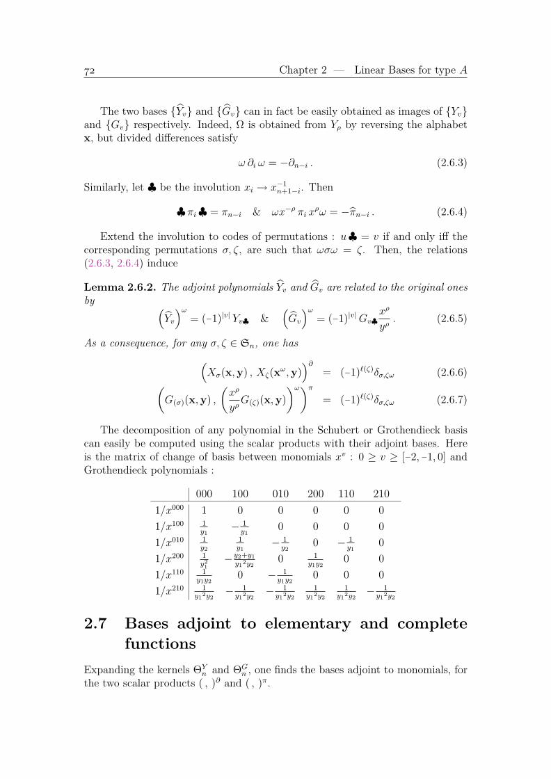
Chapter 2 — Linear Bases for type A
The two bases Yv and Gv can in fact be easily obtained as images of Yvand Gv respectively. Indeed, Ω is obtained from Yρ by reversing the alphabetx, but divided differences satisfy
ω ∂i ω = −∂n−i . (2.6.3)
Similarly, let ♣ be the involution xi → x−1n+1−i. Then
♣ πi♣ = πn−i & ωx−ρ πi xρω = −πn−i . (2.6.4)
Extend the involution to codes of permutations : u♣ = v if and only iff thecorresponding permutations σ, ζ, are such that ωσω = ζ. Then, the relations(2.6.3, 2.6.4) induce
Lemma 2.6.2. The adjoint polynomials Yv and Gv are related to the original onesby (
Yv
)ω= (−1)|v| Yv♣ &
(Gv
)ω= (−1)|v|Gv♣
xρ
yρ. (2.6.5)
As a consequence, for any σ, ζ ∈ Sn, one has(Xσ(x,y) , Xζ(x
ω,y))∂
= (−1)`(ζ)δσ,ζω (2.6.6)(G(σ)(x,y) ,
(xρ
yρG(ζ)(x,y)
)ω)π= (−1)`(ζ)δσ,ζω (2.6.7)
The decomposition of any polynomial in the Schubert or Grothendieck basiscan easily be computed using the scalar products with their adjoint bases. Hereis the matrix of change of basis between monomials xv : 0 ≥ v ≥ [−2, −1, 0] andGrothendieck polynomials :
000 100 010 200 110 210
1/x000 1 0 0 0 0 0
1/x100 1y1
− 1y1
0 0 0 0
1/x010 1y2
1y1
− 1y2
0 − 1y1
0
1/x200 1y21
−y2+y1y12y2
0 1y1y2
0 0
1/x110 1y1y2
0 − 1y1y2
0 0 0
1/x210 1y12y2
− 1y12y2
− 1y12y2
1y12y2
1y12y2
− 1y12y2
2.7 Bases adjoint to elementary and completefunctions
Expanding the kernels ΘYn and ΘG
n , one finds the bases adjoint to monomials, forthe two scalar products ( , )∂ and ( , )π.

§ 2.7 — Bases adjoint to elementary and complete functions
Proposition 2.7.1. Given n, let x∨ = x−11 , . . . , x−1
n . Then for any u, v : u ≤ρ, v ≤ ρ one has(
Pρ−v(x) , xuω)∂
= (−1)|v|δv,u =(Pv(x
∨) , xuω)π. (2.7.1)
The basis adjoint to Hv : v ≤ ρ requires a little more work, because themonomials appearing in the expansion of Hv do not respect the condition thattheir exponent be majorized by ρ. We first some technical properties of divideddifferences.
Lemma 2.7.2. Let a, b, k, n ∈ N be such that 1 ≤ k < n, 0 ≤ a, b ≤ n−k. Then
S1b(xn − xk)Sa(xk)∂k . . . ∂1 =
(−1)b if a+b = n−k
0 otherwise(2.7.2)
Proof. One expands S1b(xn − xk) = S1b(xn) − xkS1b(xn) + · · · + (−xk)b. On the
other hand, xikSa(xk) = Sa+i(xk) −∑xu, sum over monomials xu, u ∈ Nk such
that uk ≤ i−1. The initial function is therefore equal to(S1b(xn)Sa(xk)− S1b−1(xn)Sa+1(xk)− · · ·+ (−1)bS0(xn)Sa+b(xk)
)−∑
cuxu ,
with cu ∈ Sym(xn) and uNk such that uk ≤ b−1 < n−k. The extra monomials xuare sent to 0 by ∂k . . . ∂n−1 for degree reason. The sum inside parentheses is sentto
S1b(xn)Sa−n+k(xk)− S1b−1(xn)Sa+1−n+k(xk)− . . .+ (−1)bS0(xn)Sa+b−n+k(xk) = (−1)bSa+b−n+k(xn − xn) .
This last function is different from 0 only in the case S0(xn−xn) = 1, that is onlyfor a+b = n−k. QED
Proposition 2.7.3. Given n, for any v ≤ ρ, let Hv = S1v1 (xn − x1)S1v2 (xn −x2) . . . S1vn−1 (xn − xn−1). Then(
Hv , Hu
)∂= (−1)|v|δv,ρ−u , u, v ≤ ρ . (2.7.3)
Proof. Factorize ∂ω = (∂n−1)(∂n−2∂n−1) . . . (∂1 . . . ∂n−1). By decreasing inductionon k, one has to compute(
S1v1 (xn − x1) . . . S1vk (xn − xk))(Sv1(x1) . . . Svk(xk)
)∂k . . . ∂n−1
= f (S1vk (xn − xk)Svk(xk)) ∂k . . . ∂n−1 ,
with f symmetrical in xk, . . . , xn, and therefore commuting with ∂k . . . ∂n−1. Eq.2.7.2 forces the equality vk+uk = n−k, to have non nullity, and we can proceedwith k−1. QED

Chapter 2 — Linear Bases for type A
For example, for n = 3, one has the following pair of adjoint bases.
H210 = x21(x1+x2)
H110 = x1(x1+x2) H200 = x21
H100 = x1 H010 = x1+x2
H000 = 1
H000 = 1
H100 = −x2−x3 H010 = −x1−x3
H110 = (x2+x3)(x1+x3) H200 = x2x3
H210 = −x2x3(x1+x3)
2.8 Adjoint key polynomials
The two families Yv : v ∈ Nn, Gv : v ∈ Nn are bases of Pol(n) (as a vectorspace). We have also given two other bases, Kv : v ∈ Nn and Kv : v ∈ Nn,that are in fact adjoint with respect to ( , ), as states the next theorem.
First, one checks that for any partition λ, then (Kv, xλ) = 0, except when
v = λω = [λn, . . . , λ1], in which case (Kλω, xλ) = 1 (cf. [44, Cor 12]). Using that
πi is adjoint to πn−i, this allows to compute any (Kv, Ku). For example, writingin a box the non-zero scalar products, the knowledge of all (Kv, K361)
(K631, K361)
llllllllSSSSSSSS
SSSSSSSS
(K361, K361) (K613, K361)
(K316, K361)
QQQQQQQQQ(K163, K361)
llllllllllllllll
(K163, K361)

§ 2.8 — Adjoint key polynomials
determines all (Kv, K316)
(K631, K316)
mmmmmmmmmRRRRRRRR
RRRRRRRR
(K316, K316) (K613, K316)
(K316, K316)
RRRRRRRR(K163, K316)
kkkkkkkkkkkkkkkk
(K163, K316)
In conclusion, one has the following property (cf. [44, Th 15]) :
Theorem 2.8.1. Given u, v ∈ Nn, then (Kv, Ku) = 0, except (Kv, Kvω) = 1.
In particular, if λ is dominant, then (Kv, xλ) = 0, except if v = λω, in which
case Kv is a Schur function.Notice that the pairing, for Schubert and Grothendieck polynomials, is also
the reversing σ → σω, when indexing these polynomials by permutations, but notwhen using codes.

Chapter 2 — Linear Bases for type A
2.9 Reproducing kernels for Schubert and Groth-endieck polynomials
In the theory of orthogonal polynomials in one variable one finds it convenientto make use of reproducing kernels Kn(x, y) = P0(x)P0(y) + · · · + Pn(x)Pn(y),associated to a family of polynomials P0(x), P1(x), . . . of degree 0, 1, . . ., which areorthonormal with respect to a linear functional f →
∫f . The name “reproducing”
comes from the property that∫f(x)Kn(x, y) = f(y)
whenever f is a polynomial of degree ≤ n.The Cauchy kernel
∏x∈x,y∈y(1 − xy)−1 plays a similar role in the theory of
symmetric polynomials. It does not require much effort nor imagination to deducefrom the preceding section kernels corresponding to the bases Yv, Gv or Kv.Write Sym(xn) = Sym(yn) for the identification of any symmetric function of xnwith the same symmetric function of yn.
Theorem 2.9.1. For any v : 0 ≤ v ≤ ρ, one has(ΘYn , x
v)∂
= yv &(ΘGn , x
−v)π = y−v . (2.9.1)
For any Laurent polynomial f in xn, one has, modulo Sym(xn) = Sym(yn),(ΘYn , f(x)
)∂ ≡ f(y) &(ΘGn , f(x)
)π ≡ f(y) . (2.9.2)
The two kernels expand as follows
ΘYn (x, z) =
∏1≤i<j≤n
(zi − xj) =∑v≤ρ
Yv(z,y) Yρ−v(x,y) (2.9.3)
ΘGn (x, z) =
∏1≤i<j≤n
(1− xjz−1i ) =
∑v≤ρ
Gv(z,y) Gρ−v(x,y) (2.9.4)
There is no real need of a proof. The reproducing property has been obtainedin the course of proving Lemma 2.5.2. Taking coefficients in Sym(xn), one obtains(2.9.2) from (2.9.1). The function ΘY
n (x, z) belongs to the span of zuxvω : u, v ≤ρ, and therefore can be written
ΘYn (x, z) =
∑u,v
cu,v(y)Yu(z,y)Yρ−v(x,y) .
Therefore, for any v ≤ ρ, one has(ΘYn (x, z), Yv(x,y)
)∂=∑
u cu,v(y)Yu(z,y).However, the reproducing property shows that this is also equal to Yv(z,y) andthis proves (2.9.3), the case of Grothendieck polynomials being similar. QED

§ 2.10 — Cauchy formula for Schubert
For example, for n = 2, one has
ΘG2 (x, z) = 1− x2/z1 = G00(z,y)G10(x,y) +G10(z,y)G00(x,y)
= 1 ·(
1− x2
y1
)+
(1− y1
z1
)· x2
y1
.
For n = 3, Maple computes
ΘY3 (x, z) = (z1 − x2) (z1 − x3) (z2 − x3) = − (−y1 + x2) (−y1 + x3) (−y2 + x3)
+ (z2 − y2 + z1 − y1) (−y1 + x3) (−y1 + x2)− (−z1 + y2) (z1 − y1) (y1 − x3)
+ (z1 − y1) (−y2 + x3) (−y1 + x3) + (−y1 + z2) (z1 − y1) (−x2 + y2 + y1 − x3)
− (−z1 + y2) (z1 − y1) (−y1 + z2) .
The essential property of ΘYn (x,y) and ΘG
n (x,y) is that ΘYn (yσ,y) and ΘG
n (yσ,y)both vanish when σ is different from the identity. Along the same lines as for ΘY
n
and ΘGn , one sees that the kernels Yρ(x,y) and Gρ(x,y) satisfy a twisted repro-
duction property :(Yρ(x,y) , f(x)
)∂ ≡ f(yω) &(Gρ(x,y) , f(x)
)π ≡ f(yω) , (2.9.5)
modulo Sym(xn) = Sym(yn), the equivalence being replaced by an equality whenf belongs to the span of xv : [0, . . . , 0] ≤ v ≤ [0, . . . , n−1]. For example,
(G210(x,y), x23)π =
(1− y1
x1
)(1− y2
x1
)(1− y1
x2
)x2
3 π321 = y21 .
Notice that, using (2.2.4) and (2.6.5), exchanging the role of y and x, one canrewrite (2.9.4) into∑
v≤ρ
(−1)|v|Gv(x, z)Gρ−v(x,y) = Yρ(z,y)x−ρ . (2.9.6)
By taking the image of (2.9.3) under products of ∂i’s and the image of (2.9.4)
under products of πi’s, one obtains decompositions of general Yv or general Gv,and by involution, of general Yv and Gv. Let us detail these decompositions in thenext sections.
2.10 Cauchy formula for SchubertGiven u, v, w ∈ Nn, majorized by ρ, write w = u v iff and only the permutationsσ(w), σ(u), σ(v) of which they are the codes, are such that σ(w) = σ(u)σ(v) andthe product is reduced8. With this notation one has the following Cauchy formulafor Schubert polynomials (given in [97] for y = 0).
8 i.e. such that lengths add: `(σ(w)) = `(σ(u)) + `(σ(v)). Notice that the product of twopermutations η, ν is reduced if and only if ∂η∂ν = ∂ην .

Chapter 2 — Linear Bases for type A
Theorem 2.10.1. Let σ be a permutation in Sn, w ∈ Nn be its code. Then
Yw(x, z) =∑
u,v:uv=w
Yu(y, z)Yv(x,y) (2.10.1)
Xσ(x, z) =∑
η,ν: ∂η∂ν=∂σ
Xη(y, z)Xν(x,y) . (2.10.2)
Proof. One starts from the formula in the case σ = ω, which is a rewriting of (2.9.3)using (2.6.5). Supposing (2.10.2) to be true for σ, let i be such that `(σsi) < `(σ).The terms in the RHS are of two types: either `(νsi) < `(ν), or not. These lastterms are such that Xν(x,y)∂i = 0. Therefore the image of (2.10.2) under ∂i is
Xσsi(x, z) =∑
η,ζ: ∂η∂ζ=∂σsi
Xη(y, z)Xζ(x,y) ,
with ζ = νsi. QEDFor example, for w = [0, 3, 1], one has the following expansion of Y031(x, z),
writing Yu Yv for Yu(y, z)Yv(x,y)
Y031(x, z) = Y0000Y031
ssssssK
KK
Y0100Y030
KK
KY0001Y021
ssssssJJJJJJ
JJJJJJ
Y0101Y020 Y002Y011
Y012Y010
KKKKKKY03Y001
tttttttttttt
Y031Y000
,
or, indexing by permutations,
X15324(x, z) = X12345X15324
oooooooPPPP
X13245X15234
PPPPX12354X14325
oooooooPPPPPPP
PPPPPPP
X13254X14235 X12534X13425
X13524X13245
PPPPPPPX15234X12435
oooooooooooooo
X15324X12345
.
In these last conventions, the edges are simple transpositions: XηXsiζ → XηsiXζ .

§ 2.11 — Cauchy formula for Grothendieck
Notice that the above decomposition of Yρ(x, z) =∏
i+j≤n(xi − zj), becomessimilar, when specializing y = 0, to the Cauchy expansion of the resultant∏
i,j≤n(xi − zj) in terms of Schur functions in x and in z. In fact, let m, r betwo integers such that r + m < n. Then the special case of (2.10.1) for w = rm,y = 0 is
Yrm(x, z) =∑
u,v:uv=w
Yu(0, z)Yv(x,0) =∑λ≤rm
(−1)|µ|sµ(zr)sλ(xm) , (2.10.3)
sum over all pairs of partitions λ, µ such that the conjugate of µ is [r−λm, . . . , r−λ1].
2.11 Cauchy formula for GrothendieckThe analogous formula for Grothendieck polynomials is not more complicated.Instead of taking reduced products, i.e. products ∂η∂ν 6= 0, one has to use productsin the 0-Hecke algebra, of the type πηπν .
Theorem 2.11.1. Let σ be a permutation in Sn, ω = [n, . . . , 1].
G(σ)(x, z) =∑ζ∈Sn
G(ζ)(z,y)G(ωζ)(x,y) πωσ (2.11.1)
yρ
zρG(σ)(x, z) =
∑ζ
(−1)`(ζ)G(ζω)(z,y)(G(ζ)(x,y)π(ωσ)
)(2.11.2)
Proof. The first formula is the image of (2.9.4) under πωσ, the second is the imageof the case σ = ω, which is a rewriting of (2.9.6), under πωσ. QED
For example, for n = 3, writing Gv for Gv(z,y) and Gv for Gv(x,y), the imageof G210(x, z) =
∑v GvG210−v under π1 is
G110(x, z) = (G110 −G210) G000 + (G010 −G200) G010 + (G000 −G100) G110 ,
then under π2,
G100(x, z) = (G010 −G200 −G110 +G210) G000 + (G000 −G100) G100 .
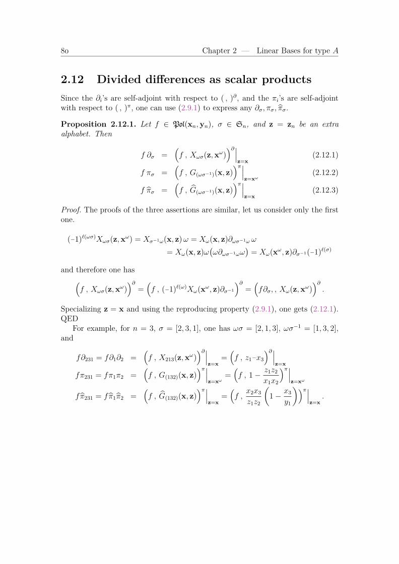
Chapter 2 — Linear Bases for type A
2.12 Divided differences as scalar productsSince the ∂i’s are self-adjoint with respect to ( , )∂, and the πi’s are self-adjointwith respect to ( , )π, one can use (2.9.1) to express any ∂σ, πσ, πσ.
Proposition 2.12.1. Let f ∈ Pol(xn,yn), σ ∈ Sn, and z = zn be an extraalphabet. Then
f ∂σ =(f , Xωσ(z,xω)
)∂∣∣∣z=x
(2.12.1)
f πσ =(f , G(ωσ−1)(x, z)
)π∣∣∣z=xω
(2.12.2)
f πσ =(f , G(ωσ−1)(x, z)
)π∣∣∣z=x
(2.12.3)
Proof. The proofs of the three assertions are similar, let us consider only the firstone.
(−1)`(ωσ)Xωσ(z,xω) = Xσ−1ω(x, z)ω = Xω(x, z)∂ωσ−1ω ω
= Xω(x, z)ω(ω∂ωσ−1ωω
)= Xω(xω, z)∂σ−1(−1)`(σ)
and therefore one has(f , Xωσ(z,xω)
)∂=(f , (−1)`(ω)Xω(xω, z)∂σ−1
)∂=(f∂σ, , Xω(z,xω)
)∂.
Specializing z = x and using the reproducing property (2.9.1), one gets (2.12.1).QED
For example, for n = 3, σ = [2, 3, 1], one has ωσ = [2, 1, 3], ωσ−1 = [1, 3, 2],and
f∂231 = f∂1∂2 =(f , X213(z,xω)
)∂∣∣∣z=x
=(f , z1−x3
)∂∣∣∣z=x
fπ231 = fπ1π2 =(f , G(132)(x, z)
)π∣∣∣z=xω
=(f , 1− z1z2
x1x2
)π∣∣∣z=xω
fπ231 = fπ1π2 =(f , G(132)(x, z)
)π∣∣∣z=x
=(f ,
x2x3
z1z2
(1− x3
y1
))π∣∣∣z=x
.

§ 2.13 — Divided differences in terms of permutations
2.13 Divided differences in terms of permuta-tions
Let D =∑
ζ∈Snζcζ(xn) be a sum of permutations with coefficients which are
rational functions in xn. Any function f(xn,yn) which vanish in all specializationsxσn = yn, except in xn = yn, can be used to determine the coefficients cζ(xn).Indeed, putting g(xn,yn) = f(xn,yn)D, one has g(xn,yn) =
∑ζ f(xζn,yn) cζ(xn),
and thereforeg(xn,x
ζn) = f(xζn,x
ζn) cζ(xn) . (2.13.1)
The kernels ΘYn ,Θ
Gn have the required vanishing properties. In consequence
the operators ∂σ, πσ, πσ can be expressed in terms of specializations of Schubert orGrothendieck polynomials, and one obtains the following expansions (the expres-sion of the coefficients are not unique, due to the many symmetries of Schubertand Grothendieck polynomials).
Proposition 2.13.1. Given σ ∈ Sn, the divided differences ∂σ, πσ, πσ are equalto the following sums of permutations :
∂σ∏i<j≤n
(xi − xj) =∑ζ≤σ
(−1)`(ζ)ζ Xωσ(xn,xζ−1ωn ) (2.13.2)
πσ =∑ζ≤σ
ζ fσ(xζ−1
n ,xωn) (2.13.3)
πσ∏i<j≤n
(1− xi
xj
)=
∑ζ≤σ
ζ G(σω)(xωn,x
ζ−1
n ) , (2.13.4)
with fσ(xn,yn) = G(ωσ−1)(xn,yn)∏
i<j≤n(1− xjx−1i )−1.
For example
∂1∂2 =(s1s2 (x1−x2)− s2 (x1−x2)− (x1−x3) s1 + (x1−x3)
) 1
∆(x3)
π1π2 = s1s2x2
3
(x1−x3)(x2−x3)− s2
x1x3
(x1−x3)(x2−x3)− s1
x22
(x1−x2)(x2−x3)
+x1x2
(x1−x2)(x2−x3)
π1π2 = (s1s2 − s2)x2
3
(x1−x3)(x2−x3)+ (1− s1)
x2x3
(x1−x2)(x2−x3).
One can compare these expressions to those given in the preceding section. In

Chapter 2 — Linear Bases for type A
fact, they can be obtained by mere expansion of
∂1∂2 = (1− s1)1
x1 − x2
(1− s2)1
x2 − x3
π1π2 =
(s1
x2
x2 − x1
+x1
x1 − x2
)(s2
x3
x3 − x2
+x2
x2 − x3
)π1π2 = (s1 − 1)
1
1− x1x−12
(s2 − 1)1
1− x2x−13
.
This is essentially the method followed by Kostant and Kumar [83, 84], but withthis method properties of the resulting coefficients are more difficult to extractthan when specializing polynomials in two sets of variables. For example we shallsee later that the inverse transition matrices, from permutations to the differenttypes of divided differences, involve the same coefficients as the transition matrices,and this fact can easily be obtained from properties of Schubert and Grothendieckpolynomials.
The leading term of πσ and πσ, i.e. the coefficient of σ, is obtained by merecommutation. Taking a reduced decomposition σ = sisjsh · · · sk, then this leadingterm is
si1
1− xix−1i+1
sj1
1− xjx−1j+1
sh · · · sk1
1− xkx−1k+1
= si · · · sk(
1
1− xix−1i+1
)sjsh···sk ( 1
1− xjx−1j+1
)sh···sk
· · · 1
1− xkx−1k+1
.
In the language of root systems, this property reads as follows.
Lemma 2.13.2. Let Φ+, Φ− be the positive (resp. negative) roots of the rootsystem of type An−1. Then, in the basis of permutations, πσ and πσ have leadingterm
F (σ) :=∏
α∈Φ+∩σΦ−
1
1− eα.
This leading term intervenes in geometry, for what concerns the postulationof Schubert varieties.
Let λ ∈ Nn be dominant weight , v be a permutation of λ, σ ∈ Sn be ofminimum length such that v = λσ. One defines the limit m→∞ of Kmvx
−mv tobe
(1− zxλ)−1πσ(1− zxv)∣∣z=x−v
.
Expanding πσ in terms of permutations, one has
(1− zxλ)−1πσ(1− zxv) = F (σ) +∑ζ<σ
1− zxv
1− zxλζcζσ ,

§ 2.14 — Schubert, Grothendieck and Demazure as commutation factors
with coefficients cζσ obtained in (2.13.3). The hypothesis on the pair λ, σ insuresthat all terms, but the first one, vanish under the specialization z = x−v. Onethus recovers in the special case of type A a property due to Peterson and Kumarin the more general context of Kac-Moody algebras.
Corollary 2.13.3. Let λ ∈ Nn be dominant, σ ∈ Sn be of minimum lengthmodulo the stabilizer of λ. Then the common limit m → ∞ of xmλπσx−mλσ andxmλπσx
−mλσ is equal to ∏α∈Φ+∩σΦ−
1
1− eα.
For example, for λ = [2, 1, 0], v = [1, 0, 2], one has σ = s1s2 and the limit ofKm,0,2mx
−m,0,−2m and Km,0,2mx−m,0,−2m is equal to
((1 − x1x
−13 )(1 − x2x
−13 ))−1.
The limit of K0,0,mx0,0,−m = Sm(x1 + x2 + x3)x−m3 = Sm(x1x
−13 + x2x
−13 + 1) is
also((1− x1x
−13 )(1− x2x
−13 ))−1, in accordance with the fact that σ is still equal
to s1s2.
2.14 Schubert, Grothendieck and Demazure ascommutation factors
One could obtain the expression of permutations in terms of divided differencesby iterating Leibnitz formula, starting with expressions like
s2s1s2 =(1 + ∂2(x3−x2)
)(1 + ∂1(x2−x1)
)(1 + ∂2(x3−x2)
).
Let us specially examine the commutation with ∂ω or πω. For example,
∂1x2 = x1∂1 − 1
∂2∂1∂2x2x23 = ∂2x3∂1x2∂2x3 = (x2∂2 − 1)(x1∂1 − 1)(x2∂2 − 1) = . . .
= x210∂2∂1∂2 − x200∂1∂2 − x110∂2∂1 + x100∂1 + (x100 + x010)∂2 − 1 .
This case shows a disymmetry which can be cured by using Schubert polynomialsinstead of monomials :
∂2∂1∂2x2x23 = Y210(x,0)∂1∂2 − Y200(x,0)∂2∂1∂2 − Y110(x,0)∂2∂1
+ Y100(x,0)∂1 + Y010(x,0)∂2 − Y000(x,0) .
The following theorem states that Schubert and Grothendieck polynomials dooccur in the commutation of some element with ∂ω or πω. Notice that this givesa generation which does not require division.

Chapter 2 — Linear Bases for type A
Theorem 2.14.1. Fixing n, with ρ = [n−1, . . . , 0], one has∑σ∈Sn
(−1)`(σ)Xσ(x,y) ∂σ−1 = ∂ωXω(y,xω) (2.14.1)∑σ∈Sn
(−1)`(σω)∂σXσ(x,y) = Xω(y,xω)∂ω (2.14.2)∑σ∈Sn
(−1)`(σ)xρG(σ)(x,y) πσ−1 = πωXω(y,xω) (2.14.3)∑σ∈Sn
(−1)`(σ)πσ G(σ)(x,y)xρ = Xω(y,xω) πω . (2.14.4)
Proof. (2.14.1) and (2.14.2) are equivalent, by left-right symmetry of the Leibnitzrelations. Let us prove (2.14.2). The factor Xω(y,xω) is the reproducing kernelΘYn , and therefore (2.14.2) can be proved by checking that, for any f(x) in the
linear span of 〈x : 0 ≤ v ≤ ρ〉, one has∑(−1)`(σ)f(x)∂σXσ(x,y) = f(y) .
Introducing an extra alphabet z, one needs a single check,
Xω(y, z) =∑σ
(−1)`(σ)Xω(x, z)∂σXσ(x,y) =∑σ
(−1)`(σ)Xωσ(x, z)Xσ(x,y) .
But this is the Cauchy formula
Xω(y, z) =∑σ
Xωσ(x, z)Xσ−1(y,x) .
Similarly, (2.14.4) is proved by checking the action on G(ω)(x, z). Thanks to(2.9.6), one has
G(ω)(x, z)∑
(−1)`(σ)πσG(σ)(x,y)xρ =∑
(−1)`(σ)G(ωσ)(x, z)G(σ)(x,y)xρ
= Xω(y, z) .
On the other hand, Xω(y,xω)y−ρ = ΘGn is a reproducing kernel with respect
to πω, and therefore, one has
G(ω)(x, z)Xω(y,xω)πω = G(ω)(y, z)yρ .
In final, the images of G(ω)(x, z) under the two sides of (2.14.4) are equal. QEDBy specialisation of y, one obtains the following commutations :∑
(−1)`(σ)∂σXσ(x,0) = x01...n−1 ∂ω (2.14.5)∑(−1)`(σ)xρG(σ)(x,1) πσ−1 = πω (1−x2) . . . (1−xn)n−1 . (2.14.6)
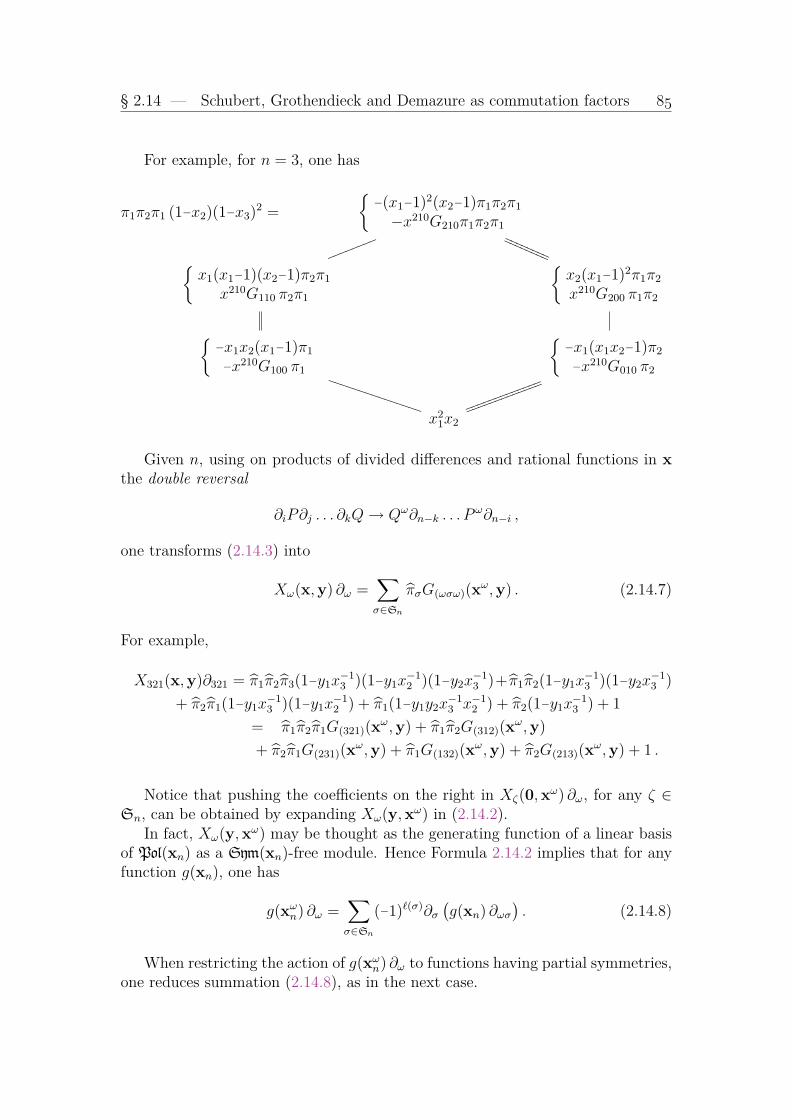
§ 2.14 — Schubert, Grothendieck and Demazure as commutation factors
For example, for n = 3, one has
π1π2π1 (1−x2)(1−x3)2 =
−(x1−1)2(x2−1)π1π2π1
−x210G210π1π2π1
llllllllQQQQQQQQ
QQQQQQQQx1(x1−1)(x2−1)π2π1
x210G110 π2π1
x2(x1−1)2π1π2
x210G200 π1π2
−x1x2(x1−1)π1
−x210G100 π1
TTTTTTTTTTTTTTT
−x1(x1x2−1)π2
−x210G010 π2
kkkkkkkkkkkkk
kkkkkkkkkkkkk
x21x2
Given n, using on products of divided differences and rational functions in xthe double reversal
∂iP∂j . . . ∂kQ→ Qω∂n−k . . . Pω∂n−i ,
one transforms (2.14.3) into
Xω(x,y) ∂ω =∑σ∈Sn
πσG(ωσω)(xω,y) . (2.14.7)
For example,
X321(x,y)∂321 = π1π2π3(1−y1x−13 )(1−y1x
−12 )(1−y2x
−13 )+ π1π2(1−y1x
−13 )(1−y2x
−13 )
+ π2π1(1−y1x−13 )(1−y1x
−12 ) + π1(1−y1y2x
−13 x−1
2 ) + π2(1−y1x−13 ) + 1
= π1π2π1G(321)(xω,y) + π1π2G(312)(x
ω,y)
+ π2π1G(231)(xω,y) + π1G(132)(x
ω,y) + π2G(213)(xω,y) + 1 .
Notice that pushing the coefficients on the right in Xζ(0,xω) ∂ω, for any ζ ∈
Sn, can be obtained by expanding Xω(y,xω) in (2.14.2).In fact, Xω(y,xω) may be thought as the generating function of a linear basis
of Pol(xn) as a Sym(xn)-free module. Hence Formula 2.14.2 implies that for anyfunction g(xn), one has
g(xωn) ∂ω =∑σ∈Sn
(−1)`(σ)∂σ(g(xn) ∂ωσ
). (2.14.8)
When restricting the action of g(xωn) ∂ω to functions having partial symmetries,one reduces summation (2.14.8), as in the next case.

Chapter 2 — Linear Bases for type A
Corollary 2.14.2. Let m ≤ n, r = n−m, k ≥ 0. For any partition λ ≤ rm,denote
∂λ =(∂m . . . ∂m+λ1−1
). . .(∂1 . . . ∂λm−1
).
Then the restriction of the action of Ykr(xω,y) ∂rm to Sym(m, r) is equal to
Ykr(xω,y) ∂r
m
=∑λ≤rm
(−1)|µ|∂λ Y0µr ,k−µr,0µr−1−µr ,k−µr−1,...,0µ1−µ2 ,k−µ1(x,y) ,
(2.14.9)denoting by µ the partition which is conjugate to [r−λm, . . . , r−λ1].
Proof. The operators Xω(xω,y)∂ω and Ykr(xω,y) ∂r
m have the same action onSym(m, r), up to sign. Moreover, the permutations σ which are not minimal intheir coset (Sm×Sr)σ annihilate elements of Sym(m, r), and therefore disappearfrom summation (2.14.8). QED
For example, for n = 5,m = 2, writing 2 3 ··1 ··
for (∂2∂3 . . . )(∂1 . . . ), one has
Y666(xω,y) 2 3 41 2 3
= 2 3 41 2 3
Y666 − 2 3 41 2
Y6605 + 2 31 2
Y66004
+ 2 3 41
Y6055 − 2 31
Y60504 − 2 3 4 Y0555 + 21Y60044
+ 2 3 Y05504 − 2 Y05044 + Y00444 .
Formula 2.14.4 :∑σ∈Sn
(−1)`(σ)πσ G(σ)(x,y) = Xω(y,xω) πωx−ρ
can be rewritten∑σ∈Sn
(−1)`(σ)πσ
(G(ω)(x,y)πωσ
)= (−1)`(ω)xρωG(ω)(x
ω,y)πωx−ρ ,
and implies that, for any function g(xn), one has∑σ∈Sn
(−1)`(ωσ)πσ
(g(xn)πωσ
)= xρωg(xωn) πωx
−ρ = g(xωn) πω . (2.14.10)
Using, thanks to (2.6.4), that πσ = (−1)`(σ)xρω πωσω ωx−ρ, putting ζ = ωσω,
h = (xρg)ω, this last equation can be transformed into∑σ∈Sn
(−1)`(ωσ)πσ
(h(xn)πωσ
)= h(xωn) πω . (2.14.11)
Taking g(xn) = xλ = h(xn), with λ dominant, one obtains key polynomials bycommutation :

§ 2.14 — Schubert, Grothendieck and Demazure as commutation factors
Theorem 2.14.3. Given an integer n and a partition λ ∈ Nn, then one has∑σ∈Sn
(−1)`(σ)πωσ(Kλπσ
)=
(xρ+λ
)ωπωx
−ρ (2.14.12)∑σ∈Sn, σ min
(−1)`(σ)πωσ Kλσ = xλω πω , (2.14.13)
the sum being limited, in the second expression, to the permutations minimum intheir coset modulo the stabilizer of λ.
For example, for λ = [3, 1, 0], one has
π2π1π2K310 − π1π2K130 − π2π1K301 + π1K103 + π2K031 −K013
= x025 π321/x210 ,
and for λ = [1, 0, 0], one has
π1π2π1 K100 − π1π2 K010 + π1K001 = x001 π321 .
Using (1.4.8), one rewrites (2.14.13) into the following commutation of πω witha dominant monomial :
πω xλ =
∑σ∈Sn, σ min
Kλσ(xω)πωσ , (2.14.14)
sum over all permutations σ which are of minimum length in their coset modulothe stabilizer of λ.
For example,
π1π2π1 x21 = x002π1π2π1 +
(x020 + x011
)π1π2 +
(x200 + x110 + x101
)π2
= K2(xω)π1π2π1 + K02(xω)π1π2 + K002(xω)π2 .
Taking in (2.14.10) g(xn) = Gλ(x,y), with λ dominant, one obtains againGrothendieck polynomials by commutation :
Gλ(xω,y) πω =
∑σ∈Sn
(−1)`(σ)πσ−1ω
(Gλ(x,y)πσ
). (2.14.15)
For example, for λ = [1, 1, 0], one has(1− y1x
−12
) (1− y1x
−13
)π321 = (π2π1π2 − π1π2)
(1− y1x
−11
) (1− y1x
−12
)+ (−π2π1 + π1)
(1− y1x
−11
)+ (π2 − 1)
= (π2π1π2 − π1π2)G110 + (−π2π1 + π1)G100 + (π2 − 1)G000 .
Thanks to the symmetry (1.4.8), one deduces from the preceding formula theexpression of the product of πω with a dominant Grothendieck polynomial in termsof πσ:
πω G(λ(x,y) =∑
σ∈Sn
(Gλ(x,y)πσ
)ωπωσ−1 . (2.14.16)

Chapter 2 — Linear Bases for type A
For example, for n = 3, one has
π321G210(x,y) = G210(xω,y) π1π2π1 +G200(xω,y) π2π1 +G110(xω,y) π1π2
+G010(xω,y) π1 +G100(xω,y) π2 +G000(xω,y) .
The expression of πωGλ(x, y) can be reduced when λ has repeated parts, i.e.when there exists i such that Gλ(x, y)πi = Gλ(x, y). Thus
π321G110(x,y) = G110(xω,y) π1π2π1 +G100(xω,y) π2π1 +G110(xω,y) π1π2
+G000(xω,y) π1 +G100(xω,y) π2 +G000(xω,y)
can be written, by right multiplication with π1, as
π321G110(x,y) = G110(xω,y) π1π2π1 +G100(xω,y) π2π1 +G000(xω,y)π1 .

§ 2.15 — Cauchy formula for key polynomials
2.15 Cauchy formula for key polynomialsThe usual Cauchy formula is the expansion of
∏i,j≤n(1−xiyj)−1 in terms of Schur
functions. We are going to see that “half” the Cauchy kernel∏
i+j≤n+1(1−xiyj)−1
expands in terms of key polynomials.Notice first that
1
(1− x1y1)(1− x1x2y1y2) · · · (1− x1 · · ·xny1 · · · yn)=∑λ
xλyλ
is the generating function of dominant monomials xλyλ in x and y. Its imageunder the product of the two symmetrizers πx
ω πyω transforms this equality into∏
i,j≤n
(1− xiyj)−1 =∑λ
Sλ(x)Sλ(y) .
We can use the same starting point, but symmetrize partially in x and y. LetΞn :=
∑σ∈Sn
πxσ πyσω. Filtering the set of permutations according to the position
of n, one gets the following factorization (we refer to [44] for more details).
Lemma 2.15.1. We have
Ξn = Ξn−1
(n−1∑i=0
πx[n−1:i] πy[n−1:n−1−i]
), (2.15.1)
where π[n−1:i] := πn−1 πn−2 · · · πn−i.
For example, the element Ξ4 factorizes as
Ξ4 = Ξ3 (πy3πy2π
y1 + πx3π
y3π
y2 + πx3 π
x2π
y3 + πx3 π
x2 π
x1 ) .
From the definition of key polynomials, the image under Ξn of∑
λ xλyλ is
equal to a sum of products of Kv(y), Ku(x). More precisely∑λ
xλyλ Ξn =∑v
Kv(y)Kvω(x) .
Using no more, but repeatedly, that
f(1− xig)−1πxi = f(1− xig)−1(1− xi+1g)−1
when f, g belong to Sym(xi, xi+1), one checks that the image of (1− x1y1)−1(1−x1x2y1y2)−1 · · · under Ξn is equal to
∏i+j≤n+1(1−xiyj)−1 [44, Prop 3]. Hence the
following kernel.
Theorem 2.15.2. For every n one has∏i+j≤n+1
(1− xiyj)−1 =∑v∈Nn
Kv(y)Kvω(x) .

Chapter 2 — Linear Bases for type A
For example, for n = 2, one has
1
(1− x1y1)(1− x1x2y1y2)(πy1+πx1 ) =
1
(1− x1y1)(1− x1y2)+
y1x2
(1− x1y1)(1− x2y1)
=1
(1− x1y1)(1− x1y2)(1− x2y1)= 1 +
∑i≤j
Kij(y)xji +∑j>i
yjiKij(x) ,
the key polynomialsKij(y) being Schur functions in y1, y2, while Kij(x) = Kij(x)−xji, when i ≤ j.

§ 2.16 — π and π-reproducing kernels
2.16 π and π-reproducing kernelsWe have shown in (2.9.2) a reproducing property of the operator f → (f , ΘG
n )π.Let us rewrite it without using the scalar product ( , )π. Let
bπΘGn =
∑σ∈Sn
πσ−1 G(σ)(z,x) (2.16.1)
πΘGn =
∑σ∈Sn
πσ−1 G(σ)(z,xω) (2.16.2)
For example, for n = 3, one has
bπΘG3 = 1 + π1
(1− x1
z1
)+ π2
(1− x1x2
z1z2
)+ π1π2
(1− x1
z1
)(1− x2
z1
)+ π2π1
(1− x1
z1
)(1− x1
z2
)+ π1π2π1
(1− x1
z1
)(1− x2
z1
)(1− x1
z2
).
With the alphabets z,xω,y instead of x,y, z, Formula 2.9.4 reads
ΘGn =
∑v≤ρ
Gv(y,xω)Gρ−v(z,x
ω) .
Indexing by permutations, using the symmetry G(σ)(x, y∨)♣ = G(σ−1)(y,x
ω) givenin (2.2.4), and the conjugation ♣πi♣ = πn−i, one rewrites this last formula as
ΘGn (z,y) =
∑v≤ρ
ΘGn (x,y)πσ−1 G(σ)(z,x
ω) (2.16.3)
= ΘGn (x,y) πΘG
n , (2.16.4)
In other words, for any v : [0, . . . , 0] ≤ v ≤ [0, . . . , n−1] = ρω, one has thereproducing property xv πΘG
n = zv. Equivalently, (2.16.4) rewrites as
Gρ(x,y) πΘGn = Gρ(z,y) . (2.16.5)
A similar computation shows that for 0 ≤ v ≤ ρ, one has x−v bπΘGn = z−v, or,
equivalently,Gρ(x,y) bπΘG
n = Gρ(z,y) . (2.16.6)These two sets of monomials are bases of Pol(xn) as a free Sym(xn)-module,
and therefore the reproducing property extends to the full space, after identifyingSym(xn) and Sym(zn). In final, one has
Proposition 2.16.1. For any f ∈ Pol(xn) one has
f(xn)πΘGn ≡ f(zn) ≡ f(xn)bπΘG
n , (2.16.7)
modulo Sym(xn) = Sym(zn).

Chapter 2 — Linear Bases for type A
Notice that the two operators πΘGn and bπΘG
n are not equal. Thus
x2bπΘG
2 = x2
(1 + π1(1− x1
z1
)
)= x1x2z
−11 ,
x2πΘG
2 = x2
(z2
x2
+ π1(1− z2
x2
)
)= z2 ,
evaluating modulo Sym(x2) = Sym(z2) being necessary to insure equality.Notice also that the two formulas xv πΘG
n = zv for 0 ≤ v ≤ ρω and x−v bπΘGn =
z−v for 0 ≤ v ≤ ρ show that both operators πΘGn and bπΘG
n take values in Sym(xn)⊗Pol(zn).
In the case n = 2, one can rewrite bπΘG2 = π1 − ∂1
x1x2
z1, πΘG
2 = π1 − ∂1z2. Thisprompts us to define, for any i,
θi = πi − ∂ixixi+1
zi& θi = πi − ∂izi+1 .
These operators do not satisfy the braid relations if the parameters zi are not allequal. Let us show however, that one can use them to factorize bπΘG
n and πΘGn .
The action of θ2θ1θ2 on G210(x,y) is such that each step is of the type (1 −xi+1y
−1j )fθi = (1 − zi+1y
−1j )f , with f symmetrical in xi, xi+1. Therefore one has
G210(x,y)θ2θ1θ2 = G210(z,y), and, more generally,
Gρ(x,y) (θn−1)(θn−2θn−1) . . . (θ1 . . . θn−1) = Gρ(z,y) .
One checks similarly that
Gρ(x,y) (θ1)(θ2θ1) . . . (θn−1 . . . θ1) = Gρ(z,y) .
Hence, these two products of operators have the same action on Pol(xn) than πΘGn
and bπΘGn respectively, and one has the following proposition.
Proposition 2.16.2. Given n, one has the factorizations
πΘGn = (θn−1)(θn−2θn−1) . . . (θ1 . . . θn−1) (2.16.8)bπΘGn = (θ1)(θ2θ1) . . . (θn−1 . . . θ1) . (2.16.9)

§ 2.17 — Decompositions in the affine Hecke algebra
2.17 Decompositions in the affine Hecke algebra
The elementary constituents of all the operators that we have used so far in type Aare divided differences, together with “multiplication by elements of Rat(x)”, thering of rational functions in x. One could as well take permutations and elements ofRat(x). Indeed, the algebras generated by ∂i, i = 1 . . . n−∪Rat(xn) , or si, i =1 . . . n−∪Rat(xn) , or πi, i = 1 . . . n−∪Rat(xn), or Ti, i = 1 . . . n−∪Rat(xn)all coincide. With M.P. Schützenberger, we call it algebra of divided differences,Bourbaki prefers produit croisé de l’algèbre du groupe symétrique et de Rat(x),Kostant and Kumar use the expression smash product, and finally, the terminologyaffine Hecke algebra for type A puts the emphasis on the elements Ti.
Every element of this algebra is uniquely written as a sum∑
σ∈Sn∂σ R
∂σ,∑
σ∈Snσ Rs
σ,∑
σ∈SnπσR
πσ,∑
σ∈SnπσR
bπσ, or
∑σ∈Sn
TσRTσ respectively, choosing
to put the coefficients on the right. Symmetry properties like (1.4.8) allow to passfrom the right module structure to the left one.
We show in (3.3.1), as a consequence of the multivariate Newton interpolationformula, how to pass from divided differences to permutations using Schubertpolynomials, or conversely in (3.3.3). In fact, this type of expansions uses onlythe obvious fact that the kernel ΘY (x,y) vanish for all specializations y = xζ ,except when ζ is the identity. Instead of ΘY (x,y), one could as well use as akernel Yρ(x,y), Gρ(x,y), or Gρ(x,y), the non vanishing being obtained for theidentity or for the maximal permutation according to the choice of the kernel.
More generally, given any f(xn) ∈ Pol(xn), let Θf (x,y) = f(xn)ΘYn . Then for
any element ∇ =∑
σ σRsσ, one has Θf (x,y)∇ =
∑σ Θf (xσ,y)Rs
σ, and thereforethe coefficients are such that
Rsσ = Θf (x,y)σ−1∇
∣∣∣y=x
1
f(xn)∆(xn).
Similar expressions hold for the other coefficients R∂σ, R
πσ, R
bπσ.
As a matter of fact, some of the formulas in preceding sections may be inter-preted as identities in the affine Hecke algebra. For example, taking z = xζ in(2.16.7), one obtains the expansion of any permutation in the basis πσ or πσ.
Let us summarize the main expansions, that will be needed later, of any ele-

Chapter 2 — Linear Bases for type A
ment ∇ of the affine Hecke algebra.
∇ =∑σ∈Sn
∂σ
(Xσ−1(x,y)∇
∣∣∣y=x
)(2.17.1)
=∑σ∈Sn
σ
( ∏1≤i<≤j≤n
(xi−yj)σ−1∇
∣∣∣y=x
)(2.17.2)
=∑σ∈Sn
πσ
(G(σ−1)(x,y
ω)∇∣∣∣y=x
)(2.17.3)
=∑σ∈Sn
πσ
(G(σ−1)(x,y)∇
∣∣∣y=x
). (2.17.4)
For example,
s1s2 =∑σ∈S3
πσ−1 Gσ(xs1s2 ,y)∣∣y=x
= 1 + π2(x3x1 − y1y2)
x3x1
+ π1
(1− y1
x3
)+ π2π1
(1− y1
x1
)(1− y1
x3
)+ π1π2
(1− y1
x3
)(1− y2
x3
)+ π1π2π1
(1− y1
x3
)(1− y2
x3
)(1− y1
x1
)∣∣∣y=x
= 1 + π2
(1− x2
x3
)+ π1
(1− x1
x3
)+ π1π2
(1− x1
x3
)(1− x2
x3
).
Specific cases of the above expansions appear in the literature. Kostant andKumar [83] consider the transition matrices σ ↔ ∂σ. Berline and Vergne[7], Arabia [1], Kostant and Kumar [84] consider the transition matrices σ ↔πσ. Kumar shows in [89] how to relate the entries of these last matrices (whichare specializations of Grothendieck polynomials) to the singularities of Schubertvarieties.
Notice that the above expansions are obtained by specializing polynomials inx,y. These polynomials are not unique. For example, instead of (2.17.3), onecould use as well
∇ =∑σ∈Sn
πσ
(G(ω)(x,y)πωσ−1∇
∣∣∣y=x
).
Let us mention in final the interest of expressing the basis of the usual Heckealgebra (with normalization (Ti−t1)(Ti−t2) = 0) in terms of the basis πσ. Forexample, for n = 3, one has
T1 = π1(x2t1 + x1t2)
x2
+ t1 & T2 = π2(x3t1 + x2t2)
x3
+ t1

§ 2.17 — Decompositions in the affine Hecke algebra
T1T2 = π1π2(x3t1+x2t2)(x1t2+x3t1)
x32 + π2
(x3t1+x2t2)t1x3
+ π1(−x1t22+x3t12)
x3+ t1
2
T2T1 = π2π1(x2t1+x1t2)(x1t2+x3t1)
x3x2+ π2
(−x1t22+x3t12)x3
+ π1t1(x2t1+x1t2)
x2+ t1
2
T1T2T1 = π1π2π1(x3t1 + x2t2) (x1t2 + x3t1) (x2t1 + x1t2)
x2x32
+ π1π2(x3t1 + x2t2) t1 (x1t2 + x3t1)
x32
+ π2π1(x2t1 + x1t2) (x1t2 + x3t1) t1
x3x2
+ π2(−x1t2
2 + x3t12) t1
x3
+ π1(−x1t2
2 + x3t12) t1
x3
+ t31 .
and these expansions specialize to the expression of permutations in the basis πσfor t1 = 1, t2 = −1, the coefficients being then specializations of Grothendieckpolynomials.

Chapter 2 — Linear Bases for type A

Chapter 3Properties of Schubert polynomials
3.1 Schubert by vanishing propertiesTo have linear bases, we could have considered only the special case where y = 0in the case of Schubert polynomials, and y = 1 in the case of Grothendieck poly-nomials. But doing so, we would lose many interesting specialization propertiesthat these polynomials possess, and that can be used to characterize them easily,as we are going to see in this section for Schubert polynomials.
Given a permutation σ (considered as an element of S∞, whose code is v), let〈v〉 = yσ = [yσ1 , . . . , yσn ].
We call 〈v〉 a spectral vector1 and write f(〈v〉)for the specialisation of f ∈
Pol(xn,y) in x1 = yσ1 , . . . , xn = yσn .
Theorem 3.1.1. Given v ∈ Nn, and σ such that v = (σ), then the Schubertpolynomial Yv(x,y) is the only polynomial in the space of degree ≤ |v| in xn suchthat
Yv(〈u〉,y) = 0 , u 6= v, |u| ≤ |v| (3.1.1)Yv(〈v〉,y
)= e(v) :=
∏i<j, σi>σj
(yσi − yσj) (3.1.2)
The specialization e(v) is called the inversion polynomial of σ. We shall alsodenote it e(σ) when no ambiguity is to be feared.Proof. First, it is straightforward that the dominant Schubert polynomials, whichare products of linear factors, satisfy both (3.1.1, 3.1.2).
1 We use the same term as for the Yang-Baxter equation, because these two uses are relatedin several ways. Notice that xs1 = [x2, x1, x3, . . .], xs1s2 = [x2, x3, x1, . . .] = [xσ1 , xσ2 , xσ3 ],with σ = s1s2 = [2, 3, 1]. We are acting on the components of the vector [x1, x2, . . .]. On theother hand, the action on the right on exponents of monomials: xσ1 = x[100]s1s2 = x001 = x3,xσ2 = x[010]s1s2 = x100 = x1, xσ3 = x[001]s1s2 = x010 = x2 involves the inverse permutation[3, 1, 2].
97

Chapter 3 — Properties of Schubert polynomials
Therefore, we have just to check the behaviour of these conditions with respectto divided differences.
Lemma 3.1.2. Let v ∈ Nn, σ = 〈v〉, i be such that vi > vi+1. Suppose that Yvsatisfies (3.1.1, 3.1.2). Then Yv ∂i also satisfies (3.1.1, 3.1.2) for the indexv′ = [v1, . . . , vi−1, vi+1, vi−1, vi+2, . . . , vn], which is the code of σsi.
Proof. Write Yv = f(xi, xi+1) − xi+1g(xi, xi+1), with f, g ∈ Sym(xi, xi+1). Let uscheck that g is the polynomial defined by (3.1.1, 3.1.2) for the index index v′.
If Yv vanishes in [xi, xi+1] = [a, b] and [xi, xi+1] = [b, a], with a 6= b, then ginherits these vanishings: g(a, b) = g(b, a) = 0. On the other hand, in the points〈v〉 and 〈v′〉, one has
Yv(〈v〉,y
)= e(v) = f(yσi , yσi+1
)− yσi+1g(yσi , yσi+1
)
Yv(〈v′〉,y
)= 0 = f(yσi , yσi+1
)− yσig(yσi , yσi+1) .
Therefore g(yσi+1, yσi) = e(v)
(yσi − yσi+1
)−1 is the inversion polynomial of σsi,and g satisfies the conditions (3.1.1, 3.1.2). This proves the lemma. But Yv∂i =−xi+1g∂i = g, and therefore g is the Schubert polynomial of index v′. This provesthe theorem. QED
For example,
Y2010(x,y) = (x1 − y1)(x1 − y2)(x2 + x3 − y1 − y2)
is characterized, among all polynomials in x1, x2, x3, x4 of degree no more than 3,by the vanishing in all x4 = yζ , ζ ∈ S4, `(ζ) ≤ 3, ζ 6= σ = [3, 1, 4, 2], and by thenormalization
Y2010(yσ,y) = (y3 − y1)(y3 − y2)(y1 + y4 − y1 − y2) = e([2, 0, 1, 0]) .
A consequence of the theorem is the following vanishing property (which evi-dent only for dominant polynomials), corresponding to 〈0〉 = [y1, y2, . . . , yn].
Corollary 3.1.3. For any v 6= [0, . . . , 0], one has Yv(y,y) = 0.
3.2 Multivariate interpolationWe have already used several times the vanishing in x = y = 〈0〉, this property isbetter understood as a special case of (3.1.1).
Notice that the polynomials Yk = (x1 − y1) · · · (x1 − yk) are the interpolationpolynomials that Newton used in his famous interpolation formula. The next the-orem states that the Schubert polynomials are precisely the universal coefficientsin the generalization of Newton’s formula to several variables (this theorem couldbe deduced from the Cauchy formula that we gave in Th. 2.10.2.

§ 3.2 — Multivariate interpolation
Given v ∈ Nn, let ∂v be any product of divided differences2 such that Yv∂v =Y0...0. It is easy to see that for any u 6= v, then Yu∂
v is either 0 or a Schubertpolynomial of index 6= [0, . . . , 0].
Theorem 3.2.1 (MultivariateNewton). For any f ∈ Pol(x,y), one has the ex-pansion
f(x) =∑v∈Nn
f(x)∂v∣∣x=y
Yv(x,y) . (3.2.1)
Proof. Test the statement on the Schubert basis. In that case, f(x)∂v is either 0 ora Schubert polynomial, whose specialization in x = y (i.e. in the point 〈0 . . . 0〉)is 6= 0 (and equal to 1) iff f(x) = Yv. QED
The preceding theorem gives the expansion of any polynomial in the Schubertbasis, the coefficients being all the non-zero images under divided differences. Inparticular, one can take the key polynomials, or the Grothendieck polynomials3.For example, the polynomial K021 has only 6 non-zero images under divided dif-ferences, the images under 1, ∂2, ∂3, ∂2∂3, ∂3∂2, ∂3∂2∂2. Writing the coefficients iny as key polynomials, one has
K021(x) = K0(y)Y0,2,1 +K0,1(y)Y0,2 +K0,1,1(y)Y0,1
+K0,0,1(y)Y0,1,1 +K0,2(y)Y0,0,1 +K0,2,1(y)Y0 .
In the case where f is a polynomial in x1 (and y) only, the only non-zerodivided differences are f∂1, f∂1∂2, f∂1∂2∂3, . . ., and the theorem is the originaltheorem of Newton, apart from notations :
f(x1) = f(y1) + f∂1 Y1 + f∂1∂2 Y2 + f∂1∂2∂3 Y3 + · · · (3.2.2)= f(y1) + f∂1(x1 − y1) + f∂1∂2(x1 − y1)(x1 − y2) + · · ·
The interpolation of functions f(x1, x2) of two variables reads
f(x1, x2) = f(y1, y2)Y00 + f∂2Y01 + f∂1Y10 + f∂2∂3Y02 + f∂2∂1Y11
+ f∂1∂2Y20 + f∂2∂3∂4Y03 + f∂2∂3∂1Y12 + f∂2∂1∂2Y21 + f∂1∂2∂3Y30 + . . .
In the case that f(x1, x2) is symmetrical, then f∂1 = 0, and only the termsYi,j, i ≤ j, which are those symmetrical in x1, x2, survive in the preceding formula:
f(x1, x2) = f(y1, y2)Y00 + f∂2Y01 + f∂2∂3Y02 + f∂2∂1Y11 + f∂2∂3∂4Y03
+ f∂2∂3∂1Y12 + f∂2∂3∂4∂5Y04 + f∂2∂3∂4∂1Y13 + f∂2∂3∂1∂2Y22 + . . .
2Take any reduced decomposition sisj · · · sk of σ, with σ of code v. Then ∂k · · · ∂j∂i is suchproduct.
3after some change of variables, like xi → 1/xi or xi → 1/(1−xi), to transform Grothendieckpolynomials into polynomials in x, and not in x−1
1 , x−12 , . . . .

Chapter 3 — Properties of Schubert polynomials
Interpolation methods can also be used in the theory of symmetric polynomials.If f(xn) belongs to Sym(xn), then only anti-dominant indices occur in the RHSof (3.2.1). In other words, Newton’s interpolation give an expansion of symmetricpolynomials in terms of Graßmannian Schubert polynomials.
For example, the Schur function s32(x3), which is equal to Y023(x,0), has thefollowing expansion in terms of Graßmannian Schubert polynomials (writing YuYvfor Yu(y,0)Yv(x,y)) :
s32(x3) = Y023(x,0) = Y000Y023 − Y00001Y022 − Y001Y013 + Y00101Y012
+ Y011Y003 − Y01101Y002 − Y00201Y011 + Y01201Y001 − Y02201Y000 .
Such expansions have been considered by Chen and Louck [20] and by Olshan-ski and Okounkov [162], in the case where y = 0, 1, 2, . . . or y = q0, q1, q2, . . .(in which case the polynomials are called factorial Schur functions).
Newton interpolation is compatible with symmetry by blocks. Indeed, letf(x) ∈ Sym(m,n, p, . . . ), i.e. f(x) is a function which is symmetrical in x1, . . . , xm,symmetrical in xm+1, . . . , xm+n, &c. Then f(x) =
∑cvYv(x,y), the set of indices
v being restricted to those such that v1 ≤ · · · ≤ vm, vm+1 ≤ · · · ≤ vm+n, &c., i.e.to those v for which Yv(x,y) belongs to Sym(m,n, p, . . . ). Otherwise, there wouldexist a divided difference ∂i annihilating f(x) and not
∑cvYv. For example, if
f ∈ Sym(3, 4, 2), then the interpolation
f(x) =∑
f(x)∂v∣∣x=y
Yv(x,y)
involves only the v ∈ N9 such that v1 ≤ v2 ≤ v3, v4 ≤ v5 ≤ v6 ≤ v7, v8 ≤ v9.
3.3 Permutations versus divided differencesFashion has changed since Newton, and it may seem of little interest to interpolatefunctions by polynomials. In fact, classical interpolation theory may be thought asa way of producing algebraic identities involving polynomials or rational functionsin several variables. In this interpretation, it still begs the right to exist, even toexpand. Moreover, one can disguise interpolation under a more sophisticatedterminology.
For example, consider the problem of expressing a permutation σ ∈ Sn, con-sidered as an operator on Pol(xn), in terms of divided differences. The image of(3.2.1) under σ is
f(xσ) =∑v∈Nn
f(x)∂v∣∣x=y
Yv(xσ,y) .
Putting y = x gives the following property obtained by Kostant and Kumar [83]in the more general context of Kac-Moody groups (they call the algebra of divideddifferences the nil Hecke ring).

§ 3.3 — Permutations versus divided differences
Proposition 3.3.1. Any permutation σ ∈ Sn expands, in terms of divided dif-ferences, as
σ =∑v≤ρ
∂v Yv(xσ,x) . (3.3.1)
For example,s2s1 = 1 + ∂2(x3 − x1) + ∂1(x2 − x1) + ∂2∂1(x3 − x1)(x2 − x1) ,
s2s1s3 = 1 + ∂1(x2 − x1) + ∂2(x4 − x1) + ∂3(x4 − x3) + ∂2∂3(x4 − x3)(x4 − x1)
+∂1∂3(x2−x1)(x4−x3)+∂2∂1(x2−x1)(x4−x1)+∂2∂1∂3(x2−x1)(x4−x1)(x4−x3) .
Conversely, one may express divided differences in terms of permutations, andmore generally, any linear combination with rational coefficients in x.Lemma 3.3.2. Let n be an integer, ΘY (x,y) :=
∏1≤i<j≤n(yi−xj) as before, and
~ =∑
σ∈Snσ hσ be a sum with rational coefficients hσ in x. Then
ΘY (x,y) ~∣∣y=xσ
= (−1)`(σ) hσ∏
1≤i<j≤n
(xi − xj) . (3.3.2)
Proof. We have already used that ΘY (x,xζ) vanishes for all permutations ζ dif-ferent from the identity. Therefore ΘY (yσ,yζ) vanishes except for ζ = σ, and thesum ΘY (x,y) ~ =
∑ΘY (xσ,y)hσ reduces to a single term when specializing y to
a permutation of x. QEDWe can take now ~ = ∂τ . Then
ΘY (x,y)∂τ = Xω(xω,y)∂τ = Xω(x,y)ω∂τω ω
= (−1)`(τ)Xω(x,y) ∂ωτ−1ωω = (−1)`(τ)Xτ−1ω(xω,y) .
In final, one has the following expression of ∂τ [108, Prop. 10.2.5] :Proposition 3.3.3. Let τ ∈ Sn. Let ∂τ =
∑ζ cτζ be the expression of ∂τ in terms
of permutations. Then
(−1)`(ζ) cτζ = (−1)`(ωτ) Xτ−1ω(xωζ ,x)1
∆(x)= Xωτ (x,x
ωζ)1
∆(x). (3.3.3)
Notice that, apart from signs and the factor ∆(x), the entries of the transitionmatrix from permutations to divided differences, and its inverse, are the same.
Here are the two transition matrices for n = 3, to be read by rows, codingx1 − x2 = 12, x1 − x3 = 13, x2 − x3 = 23 :
1 ∂2 ∂1 ∂1∂2 ∂2∂1 ∂1∂2∂1
1 1 0 0 0 0 0s2 1 23 0 0 0 0s1 1 0 12 0 0 0s2s1 1 23 13 0 23 · 13 0s1s2 1 13 12 13 · 12 0 0s1s2s1 1 13 13 12 · 13 13 · 23 12 · 13 · 23

Chapter 3 — Properties of Schubert polynomials
1 s2 s1 s1s2 s2s1 s1s2s1
∆ 12 · 13 · 23 0 0 0 0 0∂2∆ −12 · 13 12 · 13 0 0 0 0∂1∆ −13 · 23 0 13 · 23 0 0 0∂2∂1∆ 13 −13 −23 0 23 0∂1∂2∆ 13 −12 −13 12 0 0∂1∂2∂3∆ −1 1 1 −1 −1 1
Pairs of permutations τ, σ such that the specialisationXτ (xσ,x) is not a divisor
of the Vandermonde correspond singularities of Schubert varieties. There are onlytwo singularities when n = 4. One of them occurs in the expansion of ∂2∂3∂1∂2,which involves the specializations of X2143 = (x1−x2)(x1 +x2 + y3− y1− y2− y3),among which one finds (x1 − x4)2.
The full expansion of ∂2∂3∂1∂2 is
(1− s2)( x1 − x4
(x3 − x4)(x2 − x4)(x2 − x3)(−x3 + x1)(x1 − x2)
−s11
(x3−x4)(x2−x3)(−x3 + x1)(x1−x2)−s3
1
(x3−x4)(x2−x4)(x2−x3)(x1−x2)
+ s3s21
(x3−x4)(x2−x4)(x2−x3)(x1−x3)+ s1s2
1
(x2−x4)(x2−x3)(x1−x3)(x1−x2)
+ s1s31
(x3−x4)(x2−x3)(x1−x4)(x1−x2)−s1s3s2
1
(x2−x4)(x2−x3)(x1−x4)(−x3 + x1)
)The other singularity, when n = 4, occurs for ∂3∂2∂1∂2∂3, which requires spe-
cializing X1324 = x1 + x2 − y1 − y2 :
∂3∂2∂1∂2∂3 ∆ = (1− s1)(1− s3)(
(x1 +x2−x3−x4)− s2(x1−x4) + s2s3(x1−x3)
+ s2s1(x2 − x4)− s2s1s3(x2 − x3)).
On could obtain the expansion of a reduced product ∂i · · · ∂j by writing itas (1 − si)(xi − xi+1)−1 · · · (1 − sj)(xj − xj+1)−1 and enumerating all subwordsof si · · · sj. This is the method followed by Kostant and Kumar [83]. We preferrelating the coefficients to Schubert polynomials, in particular because the numberof subwords of a reduced decomposition of a permutation σ is far greater than thenumber of permutations in the interval [1, σ].
Since the coefficients cτζ in (3.3.3) must vanish when ζ does not belong to theinterval [1, τ ], one obtains the following characterization of the Ehresmann-Bruhatby vanishing properties of Schubert polynomials, which generalizes (3.1.1).
Proposition 3.3.4. Given n and two permutations σ, ζ ∈ Sn, then Xσ(xζ ,x) 6= 0if and only if σ ≤ ζ with respect to the Ehresmann-Bruhat order.
Graßmannian Schubert polynomials Yv : v ∈ Nn, v = v ↑ are symmetrical inx1, . . . , xn. One does not need to specialize them in all permutations of y1, y2, . . .,

§ 3.4 — Wronskian of symmetric functions
but, by symmetry, only in 〈u〉 = [yσ1 , . . . , yσn ] with σ of code u0 . . . 0 such thatu = u↑. In that case, the last proposition becomes :
Corollary 3.3.5. Let u, v ∈ Nn be anti-dominant. Then Yv(〈u〉,y) 6= 0 if andonly if v ≤ u (componentwise).
This property is given by Okounkov [158] in the case where y = 0, 1, 2, . . ..
3.4 Wronskian of symmetric functionsGiven a positive integer r, and r functions fi of a single variable, the determinant|fi(xj| is divisible by the Vandermonde in x1, x2, . . . , and the quotient may bethought as a discrete analogue of the Wronskian [108, Prop. 9.3.1].
Writing fi(xj) = fi(x1)s1 . . . sj−1, and using (3.3.1), one sees that∣∣fi(xj)∣∣i,j=1,...,r
∏r≥j>i≥1
(xj − xi)−1 =∣∣fix1 ∂1 . . . ∂j−1
∣∣i,j=1,...,r
.
The same formula (3.3.1) may be applied to symmetric functions, replacingthe integer r by a partition. Let λ ∈ Nn be a partition. To a family of symmetricfunctions f1(xn), f2(xn), . . . of cardinality the number of partitions contained inλ, we shall associate a Wronskian Wλ(fi).
For each µ ⊆ λ, let σµ be the Graßmannian permutation of code µ↑. Thanksto (3.3.1), every symmetric function f(xn) satisfies
f(xσµ1 , . . . , xσ
µn
)= f(xn) + · · ·+ f∂µ↑ e (σµ) .
Therefore, a determinant∣∣fi (xσµn )∣∣ may be transformed, by multiplication by a
unitriangular matrix, into the determinant∣∣fi(xn)∂
µ↑ e (σµ)∣∣.
Definition 3.4.1. Given a partition λ ∈ Nn, and a family of symmetric func-tions fi(xn) of cardinality the number N of partitions contained in λ, then theWronskian is
Wλ(fi(xn)) =∣∣fi∂µ↑∣∣i=1...N
µ⊆λ.
The preceding analysis has shown that the Wronskian is equal to
∣∣fi (xσµn )∣∣ 1∏µ⊆λ e(σµ)
.
For example, let n = 4, λ = [3, 1, 0, 0]. Then the family µ ↑, as well as theinversion polynomials e(σµ), are displayed on the next figure (writing ji insteadof xj−xi). The family ∂µ↑ is the set of paths from the origin.

Chapter 3 — Properties of Schubert polynomials
0000 ∅
0001 54
0011 43,53 0002 64,65
0012 43,63,65 0003 74,75,76
0013 43,73,75,76
∂4
∂3 ∂5
∂6∂3∂5
∂6 ∂3
In the case where the family fi(xn) is the set of Schur functions sµ(xn) :µ ⊆ λ, the Wronskian is unitriangular, and thus its determinant is equal to 1.
In the case of a rectangular partition λ ⊆ rn, the sets σµ(xn) are all thesubsets of cardinality n of x1, . . . , xn+r. Given any f ∈ Sym(xn), and i :1 ≤ i ≤ n+r−1, then the set fµ↑ is such that, either fµ↑ and fµ↑∂i occursimultaneously, or fµ↑∂i = 0. Thanks to the Leibnitz formula, this forces theWronskian Wrn(f1, f2, . . . ) to be annihilated by all ∂i, i = 1, . . . , n+r−1. In otherwords, the Wronskian is a symmetric function when λ is a rectangular partition.Moreover, any inversion (j, i), n+r ≥ j > i ≥ 1, occurs
(n+r−2n−1
)times in the set of
Graßmannian permutations σµ.In summary, one has the following lemma.
Lemma 3.4.2. Let n, r be two positive integers, let f1, . . . , fN , with N =(n+rn
),
belong to Sym(xn+r). Then
1∏n+r≥j>i≥1(xj−xi)
(n+r−2n−1 )
∣∣∣fi(X)∣∣∣ i=1...NX⊂x1,...,xn+r
= Wrn(f1, . . . , fN)
is a symmetric function of x1, . . . , xn+r.

§ 3.4 — Wronskian of symmetric functions
For example, for n = r = 2, the Wronskian
W22
(Y0(x,0), Y01(x,0), Y11(x,0), Y03(x,0), Y23(x,0), Y34(x,0)
)
=
1 ∂2 ∂2∂1 ∂2∂3 ∂2∂3∂1 ∂2∂3∂1∂2
Y0 Y0 0 0 0 0 0
Y01 Y01 Y0 0 0 0 0
Y11 Y11 Y1 Y0 0 0 0
Y03 Y03 Y002 0 Y0001 0 0
Y23 Y23 Y202 Y012 Y2001 Y0101 Y0001
Y35 Y35 Y304 Y024 Y3003 Y0203 Y0013
is equal toY0001
(Y0101Y0013 − Y0203Y0001
)= Y 2
0001Y0113 .

Chapter 3 — Properties of Schubert polynomials
3.5 Yang-Baxter and SchubertOne can degenerate Yang-Baxter bases of Hecke algebras into bases of the algebraof divided differences. However, instead of taking products of factors of the type∂i+1/c, let us take factors 1+c∂i. Accordingly, given a spectral vector [y1, . . . , yn],one defines recursively a Yang-Baxter basis f∂
σ, starting from 1 for the identitypermutation, by
f∂σsi
= f∂σ
(1 + ∂i (yσi+1
− yσi))for σi < σi+1 . (3.5.1)
For example,
f∂321 = (1 + ∂1(y2−y1))(1 + ∂2(y3−y1))(1 + ∂1(y3−y2))
= 1 + ∂1(y3−y1) + ∂2(y3−y1) + ∂1∂2(y2−y1)(y3−y1)
+ ∂2∂1(y3−y2)(y3−y1) + ∂1∂2∂2(y2−y1)(y3−y1)(y3−y2)
One remarks that the coefficients are the same as in the expression of σ =[3, 2, 1] in terms of divided differences.
The following proposition shows that this property is true in general, and thatthe coefficients are still specialisations of Schubert polynomials.
Theorem 3.5.1. The matrix of change of basis between f∂σ and ∂σ∆(y), and
its inverse, have entries which are specializations of Schubert polynomials :
f∂σ =
∑ν≤σ
∂ν Xν(yσ,y) , (3.5.2)
∂ν ∆(y) =∑
f∂σXων(y,y
ωσ) . (3.5.3)
Proof. Let σ and i be such that `(σ) < `(σsi). Suppose known the expansion
f∂σ =
∑ν
∂ν Xν(yσ,y) + ∂νsi Xνsi(y
σ,y) ,
with ν : `(ν) < `(νsi). Then its product by 1+(yσi+1−yσi)∂i is∑
ν
∂ν Xν(yσ,y) + ∂νsi
(Xνsi(y
σ,y) +Xν(yσ,y)(yσi+1
−yσi)),
and the identities
Xν(yσsi ,y) & Xνsi(y
σsi ,y) = Xνsi(yσ,y) +Xν(y
σ,y)(yσi+1−yσi)
give a similar expansion for Yσsi . QEDNotice that to expand products of factors 1 + ∂i(xi+1 − xi), one has used the
Leibnitz relations while in the present case the coefficients (in y) commute withthe operators acting on x.
The analogy between Yang-Baxter elements and permutations can be materi-alised by acting on a proper element, as shows the following proposition.

§ 3.5 — Yang-Baxter and Schubert
Proposition 3.5.2. For any σ ∈ Sn, one has
Xω(x,yω) f∂σ = Xω(x,yσω) (3.5.4)
Proof. In the step by step action of the factorised element f∂σ, each step is of the
type, f(xi − yk)(1 + ∂i(yk − yj) = f(xi − yj), f ∈ Sym(xi, xi+1). QEDFor example, for σ = [3, 4, 1, 2], writing the non-symmetric factor in a box, one
has f∂3412 =
(1 + ∂2(y3 − y2)
)(1 + ∂1(y3 − y1)
)(1 + ∂3(y4 − y2)
)(1 + ∂2(y4 − y1)
)and
x1−y2x1−y3 x2−y3x1−y4 x2−y4 x3−y4
1+∂2(y3−y2)−−−−−−→x1−y2x1−y3 x2−y2x1−y4 x2−y4 x3−y4
1+∂1(y3−y1)−−−−−−→x1−y2x1−y1 x2−y2x1−y4 x2−y4 x3−y4
1+∂3(y4−y2)−−−−−−→x1−y2x1−y1 x2−y2x1−y4 x2−y4 x3−y2
1+∂2(y4−y1)−−−−−−→x1−y2x1−y1 x2−y2x1−y4 x2−y1 x3−y2
= X4321(x,x2143) .
The general properties of Yang-Baxter bases induce properties of specialisa-tions of Schubert polynomials.
The symmetry (1.8.4) entails
(−1)`(ν)Xν(yσ,y) = Xωνω(yωσω,yω) . (3.5.5)
Each of the equations (1.8.9) and (1.8.10) gives in turn∑ν
(−1)`(ν)Xν(yσ,y)Xνω(yζ ,y) = ∆(y) δσ,ζω , (3.5.6)
but this is a special case of Cauchy formula∑ν
(−1)`(ν)Xν(yσ,y)Xνω(yζ ,y) =
∑ν
Xν−1(y,yσ)Xνω(yζ ,y) = Xω(yζ ,yσ) .
The quadratic form ( , )H defined in (1.8.5) degenerates into the form
(f , g)H00 = f g∨ ∩ ∂ω , (3.5.7)
still denoting f → f∨ be the anti-automorphism of the algebra of divided differ-ences induced by (∂σ)∨ = ∂σ−1 .
Property (1.9.5) becomes
Proposition 3.5.3. The Yang-Baxter bases associated to the spectral vectors[y1, . . . , yn] and [yn, . . . , y1] satisfy the relations(
f∂,yσ , f∂,yω
ζ
)H00
= δσ,ωζ ∆(yσ) . (3.5.8)
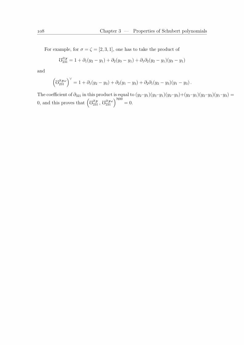
Chapter 3 — Properties of Schubert polynomials
For example, for σ = ζ = [2, 3, 1], one has to take the product of
f∂,y231 = 1 + ∂1(y2 − y1) + ∂2(y3 − y1) + ∂1∂2(y2 − y1)(y3 − y1)
and (f∂,yω
231
)∨= 1 + ∂1(y2 − y3) + ∂2(y1 − y3) + ∂2∂1(y2 − y3)(y1 − y3) .
The coefficient of ∂321 in this product is equal to (y2−y1)(y3−y1)(y2−y3)+(y2−y1)(y2−y3)(y1−y3) =
0, and this proves that(f∂,y
231 , f∂,yω231
)H00
= 0.

§ 3.6 — Distance 1 and multiplication
3.6 Distance 1 and multiplicationThe ring Sym(x) has a linear basis consisting of Schur functions. Its multiplicativestructure is determined by the Pieri formulas, i.e. by the products of Schur func-tions by the elementary (or complete) symmetric functions. In the non-symmetriccase, the requirement to recover the ring structure is easier. Polynomials beingsums of monomials, and monomials being products of variables, we need onlydescribe the images of the different bases under multiplication by x1, x2, . . ..
Our bases being obtained by the use of ∂i’s or πi’s, we could use the commu-tation properties of these operators with multiplication by a single variable.
In the case of Schubert polynomials, let us rather use interpolation methods.This time, it will be more convenient to index polynomials by permutations, pass-ing from the notation Yv to the notation Xσ, where v is the code c(σ) of σ.
Definition 3.6.1. v ∈ Nn is a successor of u if |v| = |u| + 1 & Yu(〈v〉,y) 6= 0.Given two permutations ζ, σ, then ζ is a successor of σ iff this is so for theircodes.
Theorem 3.6.2. A permutation ζ, of code v, is a successor of σ iff ζσ−1 is atransposition (a, b), and `(ζ) = `(σ) + 1. In that case,
Xσ(〈v〉,y) = e(v) (yζb − yζa)−1 .
Proof. If u = c(σ) is dominant, then it is immediate to write the specializations ofYu and check the proposition in that case. Let us therefore suppose that there ex-ists i such that ui < ui+1, and let η be such that c(η) = [u1, . . . , ui−1, ui+1+1, ui, ui+2, . . . , un].Since for any permutation ζ of code v, one has(
Xη(〈v〉,y)− (Xη(〈v〉),y)si)
(yζi − yζi+1)−1 = Xσ(〈v〉,y) ,
ζ can be a successor of σ only if ζ = η, or if ζsi is a successor of η. In the firstcase,
Xσ(〈v〉,y) = Xη(〈v〉,y)(yηi − yηi+1)−1 = e(v)) ,
while in the second,
−Xη(〈v〉si ,y)
yζi − yζi+1
=e(c(ζsi))
(yζi+1− yζi)(yζb − yζa)
=e(c(ζ))
yζb − yζa,
and this proves the proposition. QED
Corollary 3.6.3 (Monk formula [81]). Given v ∈ Nn, σ = 〈v〉, k ∈ 1, . . . , n,then
(xk − yσk)Xσ(x,y) =∑j>k
Xστk,j(x,y)−∑j<k
Xστk,j(x,y) , (3.6.1)
summed over all transpositions τk,j such that `(στk,j) = `(σ) + 1.
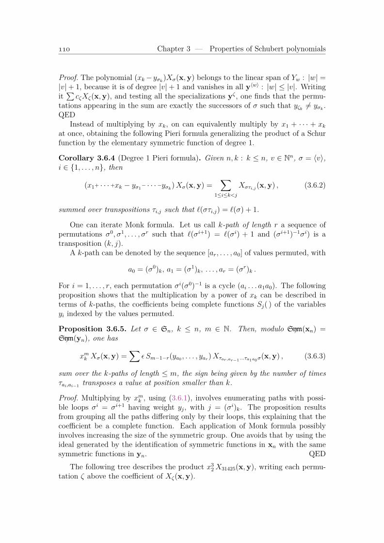
Chapter 3 — Properties of Schubert polynomials
Proof. The polynomial (xk−yσk)Xσ(x,y) belongs to the linear span of Yw : |w| =|v|+ 1, because it is of degree |v|+ 1 and vanishes in all y〈w〉 : |w| ≤ |v|. Writingit∑cζXζ(x,y), and testing all the specializations yζ , one finds that the permu-
tations appearing in the sum are exactly the successors of σ such that yζk 6= yσk .QED
Instead of multiplying by xk, on can equivalently multiply by x1 + · · · + xkat once, obtaining the following Pieri formula generalizing the product of a Schurfunction by the elementary symmetric function of degree 1.
Corollary 3.6.4 (Degree 1 Pieri formula). Given n, k : k ≤ n, v ∈ Nn, σ = 〈v〉,i ∈ 1, . . . , n, then
(x1+ · · · +xk − yσ1− · · · −yσk)Xσ(x,y) =
∑1≤i≤k<j
Xστi,j(x,y) , (3.6.2)
summed over transpositions τi,j such that `(στi,j) = `(σ) + 1.
One can iterate Monk formula. Let us call k-path of length r a sequence ofpermutations σ0, σ1, . . . , σr such that `(σi+1) = `(σi) + 1 and (σi+1)−1σi) is atransposition (k, j).
A k-path can be denoted by the sequence [ar, . . . , a0] of values permuted, with
a0 = (σ0)k, a1 = (σ1)k, . . . , ar = (σr)k .
For i = 1, . . . , r, each permutation σi(σ0)−1 is a cycle (ai . . . a1a0). The followingproposition shows that the multiplication by a power of xk can be described interms of k-paths, the coefficients being complete functions Sj( ) of the variablesyi indexed by the values permuted.
Proposition 3.6.5. Let σ ∈ Sn, k ≤ n, m ∈ N. Then, modulo Sym(xn) =Sym(yn), one has
xmk Xσ(x,y) =∑
ε Sm−1−r(ya0 , . . . , yar)Xτar,ar−1 ...τa1a0σ(x,y) , (3.6.3)
sum over the k-paths of length ≤ m, the sign being given by the number of timesτai,ai−1
transposes a value at position smaller than k.
Proof. Multiplying by xmk , using (3.6.1), involves enumerating paths with possi-ble loops σi = σi+1 having weight yj, with j = (σi)k. The proposition resultsfrom grouping all the paths differing only by their loops, this explaining that thecoefficient be a complete function. Each application of Monk formula possiblyinvolves increasing the size of the symmetric group. One avoids that by using theideal generated by the identification of symmetric functions in xn with the samesymmetric functions in yn. QED
The following tree describes the product x32X31425(x,y), writing each permu-
tation ζ above the coefficient of Xζ(x,y).

§ 3.6 — Distance 1 and multiplication
3 1 425y3
1
ttttttKKKKKK
3 2 415S2(y1, y2)
3 4 125S2(y1, y4)
MMMMMMM
3 4 215y1 + y2 + y3
JJJJJJ
4 3 125−y1 − y3 − y4
3 5 124y1 + y4 + y5
4 3 215−1
3 5 2141
4 5 123−1
5 3 124−1
or, for the readers who prefer one-dimensional formulas,
x32X31425 = y3
1X3142+(y21+y2
4+y1y4)X3412+(y21+y1y2+y2
2)X3241+(y1+y5+y4)X35124
−(y3+y1+y4)X4312+(y4+y1+y2)X3421−X45123+X361245−X53124+X35214−X4321 .

Chapter 3 — Properties of Schubert polynomials
3.7 Pieri formula for Schubert polynomialsThe Italian geometer Pieri described the intersection of a Schubert cycle by a“special” one in the cohomology ring of the Grassmannian. In modern terms, hedescribed the product of a Schur function by an elementary or complete function,the remarkable property being that there is no multiplicity in Pieri formula.
Let us generalize Pieri’s result to Schubert polynomials, the presence of extravariables y allowing to interpret the intersection numbers 1 as complete functionsof degree 0.
Our starting point will be the following case.
Lemma 3.7.1. Let n, k, r ∈ N, ρ = [n−1, . . . , 0], m = max(n−k, 0) and y♥ =ym+1, ym+2, ym+3, . . . . Then
Yρ(x,y)Y0k−1r(x, z) = Yρ(x,y)Y0k−1r(y♥, z)
+k∑i=1
r∑j=1
Yρ+[0i−1j0n−k](x,y)Y0k−1+jr−j(y♥, z) . (3.7.1)
Proof. One uses Newton’s interpolation (3.2.1) on the product fg, with f =Yρ(x,y), g = Y0k−1r(x, z), using Leibnitz’ formula (1.4.2). The images of f un-der products of divided differences are 0 or Schubert polynomials that one hasto specialize in x = y. Only Y0...0 subsists. Let us first suppose that n ≤ k.In a sum
∑εi,...εh∈0,1
(f∂εii ∂
εjj · · · ∂
εhh
)(gsεii ∂
1−εii s
εjj ∂
1−εjj · · · sεhh ∂
1−εhh
)there remains
only divided differences ∂i, i < n acting on f , si preserving g, and products∂k∂k+1 · · · ∂k+j−1 acting on g and sending it to Y0k−1+jr−j(x, z).
In final, for n = 3 = k for example, the only non-zero contributions in Newton’sformula are for ∂2∂1∂2(∂3∂4 · · · ), ∂2(∂3∂4 · · · )∂1∂2 and (∂3∂4 · · · )∂2∂1∂2, and thiscorresponds indeed to the RHS of (3.7.1).
In the case where n > k, writing y♥ = yn−k, yk+1, . . ., one factors Yρ(x, y) =Y(n−k)k,n−k−1,...,0(x,y)Yk−1,...,0(x,y♥), and write the interpolation for the productYk−1,...,0(x,y♥)Y0k−1r(x, z). QED
For example, for n = 5, k = 3, r = 2, one has y♥ = y3, y4, . . . and
Y43210(x,y)Y002(x, z) = Y43210(x,y)Y002(y♥, z) +(Y53210(x,y) + Y44210(x,y)
+ Y43310(x,y))× Y0001(y♥, z) +
(Y63210(x,y) + Y45210(x,y) + Y43410(x,y)
).
To describe the general Pieri formula, it is convenient to index Schubert poly-nomials by permutations, and generalize consecutivity in the Bruhat order.
Given an integer k, a pair of permutations σ, η : σ ≤ η is called a k-soulèvementof degree indexsoulèvement `(η)−`(σ) if each cycle ζi in the cycle-decompositionησ−1 = ζ1 · · · ζm is of the type ζi = (α, δ, γ, . . . , β) with δ > γ > · · · > β > α,δ, . . . , α ∩ σ1, . . . , σk = α and `(η) = `(σ) + (#ζ1 − 1) + · · · + (#ζm − 1).Denote furthermore yσ,η = yσ1 , . . . , yσk ∪ yi : i ∈ ζ1 ∪ · · · ∪ ζm.

§ 3.7 — Pieri formula for Schubert polynomials
For example the pair σ = [5, 2, 7, 4, 1, 6, 8, 3, 9], η = [6, 2, 9, 4, 3, 5, 7, 1, 8]) is a5-soulèvement of degree 1+1+2 = `(η)−`(σ), because ησ−1 = (1, 3)(5, 6)(7, 9, 8),and yσ,η = y5, y2, y7, y4, y1 ∪ y1, y3 ∪ y5, y6 ∪ y7, y9, y8= y5, y2, y7, y4, y1, y6, y8, y9.
Theorem 3.7.2. Let n, k, r ∈ N, σ ∈ Sn. Then
Xσ(x,y)Y0k−1r(x, z) =∑η
Xη(x,y)Y0k−1+jr−j(yσ,η, z) , (3.7.2)
sum over all k-soulèvements (σ, η) of degree j = 0, . . . , r.
Proof. The divided differences in y send Xn...1(x,y) onto any Xσ(x,y), up to sign.Thus, the theorem can be proved by decreasing induction on `(σ), checking theevolution of the RHS of (3.7.6) under a simple divided difference in y, startingfrom (3.7.1). QED
For example of the recursion, the term X3471256(x,y)Y052(y3, y1, y5, y4, y7, y6)occurs in the expansion of X31542(x,y)Y005(x, z), and the permutation[3, 4, 7, 1, 2, 5, 6][3, 1, 5, 4, 2]−1 is equal to the product of cycles (1, 4)(5, 7, 6). Under−∂y2 , this term gives, in the expansion of X21543(x,y)Y005(x, z) the two termsX3471256(x,y)Y061(y2, y1, y5, y4, y3, y7, y6) andX2471356(x,y)Y052(y2, y1, y5, y4, y7, y6), in accordance with
[3, 4, 7, 1, 2, 5, 6][2, 1, 5, 4, 3]−1 = (1, 4)(2, 3)(5, 7, 6) ,
[2, 4, 7, 1, 3, 5, 6][3, 1, 5, 4, 2]−1 = (1, 4)(5, 7, 6) .
The product of a Schubert polynomial by the elementary symmetric functionsof x1, . . . , xk can be described similarly. In fact, instead of starting by the productof Yρ(x,y) by
∑k0(x,0)(−z)k−i = Y1k(x, z) =
∏k1(xi−z), one can multiply Yv(x,y)
by∏k
1(xi−zi) under some hypothesis on v. The elementary step is the following,which transforms multiplication by xi into an action of a divided difference in y.
Let v be dominant, i = 1 or i be such that vi−1 > vi+1, v′ = v + [0i−11],j = vi+1. Then
Yv(x,y)(xi−z) = Yv′(x,y) + (yj−z)Yv(x,y) = Yv′(x,y) (z−yj+1)∂yj .
For example, for v = [4, 2, 1], i = 2, ignoring the factors which are invariant undersy2 , one has
Y421(x,y)(x2−y3)(z−y4) = x2−y3 z−y4∂y3−−→Y421(x,y)(x2−z) .

Chapter 3 — Properties of Schubert polynomials
By iteration, for an integer k and v dominant such that v1 > · · · > vk > vk+1,one has
Yv(x,y)(x1−z1) · · · (xk−zk)= Yv+1k−1(x,y)
((zk−1−yvk−1+2)∂y
vk−1+1
)· · ·((z1−yv1+2)∂y
v1+1
)(xk−zk)
= Yv+1k−1(x,y)(xk−zk)((zk−1−yvk−1+2)∂y
vk−1+1
)· · ·
= Yv+1k(x,y)((zk−yvk+2)∂y
vk+1
)· · ·((z1−yv1+2)∂y
v1+1
),
and one obtains the following lemma.
Lemma 3.7.3. Let v be dominant, k be such that v1 > · · · > vk > vk+1, u =v + [1k]. Then one has
Yv(x,y)(x1−z1) · · · (xk−zk) = Yu(x,y)(zk−yuk+1)∂yuk· · · (z1−yu1+1)∂y
u1
= Yu(x,y)(zk−yuk+1) · · · (z1−yu1+1)∂yuk· · · ∂y
u1. (3.7.3)
As a corollary, one has, for ρ = [n−1, . . . , 0] and k ≤ n,
Yρ(x,y)Y1k(y, z) =∑
0k≤u≤1k
Yρ+1k−u(x,y)(yn−z1)u1 · · · (yn−k+1−z1)uk . (3.7.4)
Using the divided differences in z, this formula implies the following analog of(3.7.1).
Lemma 3.7.4. Let n, r, k be three integers, 0 ≤ r ≤ k ≤ n, ρ = [n−1, . . . , 0]. Foru ∈ [0, 1]k, denote y〈u〉 = yn+1−i : i such that ui = 1, 1 ≤ i ≤ k. Then
Yρ(x,y)Y0r1k−r(y, z)
=∑
0k≤u≤1k
(−1)|u|−rYρ+1k−u(x,y)S|u]−r(z1+ · · · +zr+1 − y〈u〉) . (3.7.5)
For example,
Y4321(x,y)Y011(x, z) = Y4431(x,y) + Y5331(x,y) + Y5421(x,y)
− Y5321(x,y)(z1+z2 − y4−y3)− Y4421(x,y)(z1+z2 − y5−y3)
− Y4331(x,y)(z1+z2 − y5−y4) + Y4321(x,y)S2(z1+z2 − y5−y4−y3) .
The general product Yv(x,y)Y0r1k−r(x, z) requires mirroring the notion of souléve-ment. Given an integer k, a pair of permutations σ, η : σ ≤ η is called a k-soulèvement gauche of degree `(η)−`(σ) if each cycle ζi in the cycle-decompositionησ−1 = ζ1 · · · ζm is of the type ζi = ((α, β, γ, . . . , δ) with α < β < γ · · · < δ,α, . . . , δ∩σ1, . . . , σk = δ, and `(η) = `(σ)+(#ζ1−1)+ · · ·+(#ζm−1). Fora pair (σ, η) of permutations, denote y[σ,η] = yσ1 , . . . , yσk ∩ yη1 , . . . , yηk. Thenone has the following Pieri formula for multiplication by elementary symmetricfunctions.
§ 3.7 — Pieri formula for Schubert polynomials
Theorem 3.7.5. Let n, k, r ∈ N, 0 ≤ r ≤ k ≤ n, σ ∈ Sn. Then
Xσ(x,y)Y0r1k−r(x, z) =∑η
(−1)k−r+`(σ)−`(η) Xη(x,y)Sk−r+`(σ)−`(η)(zr+1 − y[σ,η]) ,
(3.7.6)sum over all k-soulèvements gauches (σ, η) of degree j = 0, . . . , r.
For example, in the product Y241596837(x,y)Y0111(x, z), one has the term−Y34195827(x,y)(z1+z2−y1−y4), the cycle decomposition of ησ−1 being (2, 3)(5, 9),and the intersection yσ1 , . . . , yσ4 ∩ yη1 , . . . , yη4 being y1, y4.
Chapter 3 — Properties of Schubert polynomials
3.8 Products of Schubert polynomials by oper-ators on y
We have described in the preceding sections Pieri multiplications by the combina-torics of soulèvements. Let us rather use now operators in y. For example, the ele-mentary products Y201(x,0)Y11(x,0) = Y32(x,0)+Y311(x,0), Y101(x,0)Y11(x,0) =Y31(x,0) + Y22(x,0) + Y211(x,0) can be rewritten
Y201(x,0)Y11(x,0) = Y321(x,0)(−∂y1 −∂
y2 )
Y101(x,0)Y11(x,0) = Y321(x,0)(−∂y1 −∂
y2 )(−∂y
2 −∂y3 )
= Y321(x,0)(∂y
1 ∂y2 + ∂y
1 ∂y3 + ∂y
2 ∂y3
),
indicating that the elements δi = ∂i + ∂i+1 play a role in the multiplication ofSchubert polynomials.
For them, the braid relations of order 3 are still valid:
δiδi+1δi = δi+1δiδi+1 = (∂i∂i+1+∂i∂i+2+∂i+1∂i+2)∂i + (∂i∂i+2+∂i+1∂i+2)∂i+1 .
In the case of order 2, one has δiδj = δjδi if |j−i| > 2, but
δiδi+2 − δi+2δi = ∂i+1∂i+2 − ∂i+2∂i+1 .
Note, however, that the elements δi do not satisfy a Hecke relation, but that
δ2i = ∂i∂i+1 + ∂i+1∂i , δ
3i = 2∂i∂i+1∂i , δ
4i = 0 .
Given two positive numbers r, p, let ϕ([r], p) = δp · · · δp+r−1, and for a partitionλ ∈ N`, let
ϕ(λ, p) = ϕ([λ1], p)ϕ([λ2], p−1) · · ·ϕ([λ`], p−`+1) . (3.8.1)
For example, the product ϕ([3, 3, 1], 3) is obtained by reading by the successiverows of the display
δ3 δ4 δ5δ2 δ3 δ4δ1
. In fact, one easily checks that δ1, δ2, . . . satisfy thenilplactic relations (cf. 6.9.1)
δiδi+1δi−1 = δiδi−1δi+1 ,
and this allows to pass from the row-reading of the array to its column-reading.Hence ϕ([3, 3, 1], 3) is also equal to (δ3δ2δ1)(δ4δ3)(δ5δ4).
By induction on r, one checks that
ϕ([r], p) =
p+r∑j=p
(∂p · · · ∂j−1)(∂j+1 · · · ∂p+r) .
We shall not use the fact that, more generally, the non-zero terms in the expansionof ϕ(λ, p) are in bijection with the partitions whose diagram is contained in the
§ 3.8 — Products of Schubert polynomials by operators on y
diagram of λ. For example, reading the diagrams by rows, i standing for ∂i, one has9 terms in the expansion of ϕ([3, 2], 2). The partitions are obtained by reorderingthe lengths of the rows of the left part of diagram (as cut by the bullets).
ϕ([3, 2], 2) =• 3 4 5• 2 3∅
+• 3 4 51 • 3
1+
2 • 4 51 • 3
11+• 3 4 51 2 •
2
+2 • 4 51 2 •
21+
2 3 4 •• 2 3
3+
2 3 • 51 2 •
22+
2 3 4 •1 • 3
31+
2 3 4 •1 2 •
32
When v is dominant, and i is such that vi−1 > vi+1 (or i = 1), then
Yv(x,y)(xi−z) = Yu(x,y) + (yui−z)Yv(x,y) = Yu(x,y)(1 + ∂y
ui(z−yui)
), (3.8.2)
with u = v + [0i−1, 1]. One has therefore to introduce the operators
Di(z) = 1 + ∂yi (z − yi)
depending on extra indeterminates z.Let us show that these operators allow to express the product of two dominant
Schubert polynomials Yλ(x,y)Yµ(x, z). We have first to reinterpret the construc-tion of the canonical reduced decomposition of a permutation from its code. Letu ∈ N`. Fill the diagram of u by consecutive numbers upwards in each column,starting with the column number at the bottom, as in section 1.1. Then Du(z) isthe product obtained by reading the diagram by successive columns, from top tobottom, interpreting an entry i at level j as Di(zj). For example, u = [3, 0, 1, 2]
gives the diagram32 51 3 4
and the product
D3012(z) =(D3(z3)D2(z2)D1(z1)
)( )(D3(z1)
)(D5(z2)D4(z1)
).
Decomposing Yµ(x, z) into products of factors of the type (x1−zj) · · · (xk−zj),and applying repeatedly remark (3.8.2), one obtains the following description ofthe product of two dominant Schubert polynomials.Proposition 3.8.1. Let λ, µ be dominant, ζ be the permutation of code λ+µ, σbe the permutation of code λ, and u be the code of ζσ−1. Then
Yλ(x,y)Yµ(x, z) = Yλ+µ(x,y)Du(z) . (3.8.3)
For example, for λ = [4, 3, 3, 2, 1], µ = [2, 2, 1, 1], one has λ+µ = [6, 5, 4, 3, 1],ζ = [7, 6, 5, 4, 2, 1, 3], σ = [5, 4, 6, 3, 2, 1], ζσ−1 = [1, 2, 4, 6, 7, 5, 3], u = [0, 0, 1, 2, 2, 1],and Du(z) = D3(z1) ·D5(z2)D4(z1) ·D6(z2)D5(z1) ·D6(z1). Hence
Y43321(x,y)Y2211(x, z) = Y65431(x,y)D3(z1)D5(z2)D4(z1)D6(z2)D5(z1)D6(z1) .
We are now in position to rewrite the product of a Schubert polynomial by anelementary symmetric function, ϕy(λ, p) standing for a product of operators on yinstead of x.

Chapter 3 — Properties of Schubert polynomials
Proposition 3.8.2. Let k ∈ N, σ ∈ Sn such4 that n 6∈ σ1, . . . , σk, v be thecode of σ, ζ be the permutation of maximal length in the coset σSk|n−k. Letλ be the partition #i : ζi < ζj, i = 1, . . . , k, j = k+2, . . . , n. Let moreoveru = [σ1, . . . , σk] ↑. Then
Xσ(x,y)Y1k(x, z) = (−1)|λ|Xωζ−1σ(x,y)ϕy(λ, n−k−1)Du1(z1) · · ·Duk(z1) . (3.8.4)
Proof. . One first shows that
Xζ(x,y)Y1k(x, z) = (−1)|λ|Xω(x,y)ϕy(λ, n−k−1)Du1(z1) · · ·Duk(z1) ,
by induction on the last part of λ. Since ∂xζ−1σ commutes with Y1k(x, z), one has
Xσ(x,y)Y1k(x, z) = Xζ(x,y)Y1k(x, z)∂xζ−1σ
= (−1)|λ|Xω(x,y) ∂xζ−1σϕ
y(λ, n−k−1)Du1(z1) · · ·Duk(z1)
= (−1)|λ|Xωζ−1σ(x,y)ϕy(λ, n−k−1)Du1(z1) · · ·Duk(z1) .
QEDFor example, for σ = [1, 4, 2, 5, 3], k = 3, one has ζ = [4, 2, 1, 5, 3], ωζ−1σ =
[3, 5, 4, 2, 1], λ = [2], and
X14253(x,y)Y111(x, z) = X35421(x,y)(∂y1 ∂
y2 + ∂y
1 ∂y3 + ∂y
2 ∂y3 )D1(z1)D2(z1)D4(z1)
=(X25413(x,y) +X25341(x,y)
)D1(z1)D2(z1)D4(z1)
= X25413 +X25341 +(y4−z1)X24513 +(y1−z1)X15342 +(y4−z1)X24351 +(y1−z1)X15423
+ (y4−z1) (y1−z1)X14352 + (y2−z1) (y1−z1)X15243
+ (y4−z1) (y1−z1)X14523 + (y4−z1) (y2−z1) (y1−z1)X14253 .
One can rewrite the preceding formula using that
Xωζ−1σ(x,y) = (−1)`(σ)+`(ζ)Xω(x,y)∂yωσ−1ζω ,
so as to start from a dominant polynomial.Combining with formula (3.8.3) expressing the product of two dominant Schu-
bert polynomials, one obtains the product of a general Schubert polynomial by adominant one in x, z, and by using divided differences in z, the product of twoSchubert polynomials.
Theorem 3.8.3. With the notations of (3.8.4), let ρ = [n−1, . . . , 0], ω = [n, . . . , 1].Let moreover µ be a partition of length k, η = µ−1k, ξ be the permutation of codeρ+η, and finally w be the code of ξω. Then
Xσ(x,y)Yµ(x, z) = (−1)|λ|+`(σ)+`(ζ)Yρ+ηDw(z2, . . . , zµ1)
∂yωσ−1ζωϕ
y(λ, n−k−1)Du1(z1) · · ·Duk(z1) . (3.8.5)4if not, one adds a fixed point n+1 to σ.

§ 3.8 — Products of Schubert polynomials by operators on y
Let v be such that there exists a permutation ν such that Yµ(x, z)∂zν = (−1)`(ν)Yv(x, z).
Then
Xσ(x,y)Yv(x, z) = (−1)|λ|+`(σ)+`(ζ)+`(ν)Yρ+ηDw(z2, . . . , zµ1)
∂yωσ−1ζωϕ
y(λ, n−k−1)Du1(z1) · · ·Duk(z1) ∂zν . (3.8.6)
Continuing the preceding example, one has
X14253(x,y)Y331(x, z) = Y4321(x,y)∂y4 ∂
y3ϕ([2], 1)D1(z1)D2(z1)D4(z1)Y22(x, z2, z3)
= Y6521(x,y)D5(z3)D6(z3)D4(z2)D5(z2)∂y4 ∂
y3ϕ([2], 1)D1(z1)D2(z1)D4(z1) .
The image of this equation under ∂z3 gives a non-dominant product:
−X14253(x,y)Y231(x, z) = Y6521(x,y)(∂y
5 +∂y6 +∂y
5 ∂y6 (z3+z4−y5−y6)
)D4(z2)D5(z2)∂y
4 ∂y3ϕ([2], 1)D1(z1)D2(z1)D4(z1) .
Formula (3.8.6) for the product of two Schubert polynomials involves us-ing divided differences in z. Thanks to Leibnitz, one needs only to know thatDj(zi)∂
zi = ∂y
j and Dj(zi+1)∂zi = −∂y
j to eliminate the divided differences in z. Inall, the product of two Schubert polynomials Xσ(x,0)Yv(x,0) in x only is com-puted by starting from a dominant ancestor Yµ(x, z) of Yv(x, z), taking the imageof (3.8.5) under an appropriate product of divided differences in z, then specializ-ing all zi to 0, i.e. replacing all Dj(zi) by Dj(0) = 1− ∂y
j yj = −yj+1∂j. However,evaluating a mixture of ∂y
i and yi+1∂yi is not straightforward.
Let us follow another strategy by first pushing all the operators Dj(zi) to theright, iterating the Pieri formula.
First notice that (3.8.4) implies that the expression
Xσ(x,0)x1 · · ·xk =∑
Xζ(x,0)
extends to
Xσ(x,y)Y1k(x, z) =∑
Xζ(x,y)Du1(z1) · · ·Duk(z1) .
Moreover, since u1, . . . , uk is increasing, coefficients can be pushed to the rightand the product Du1(z1) · · ·Duk(z1) is equal to∑
εi=0,1
(∂yu1
)ε1 · · · (∂yuk
)εk(z1−yu1)ε1 · · · (z1−yuk)
εk .
For a given ζ, some ∂yi possibly annihilate Xζ(x,y). Thus there exists a minimal
subsequence uζσ = [v1, . . . , vr] of [u1, . . . , uk] such that
Xζ(x,y)Du1(z1) · · ·Duk(z1) = Xζ(x,y)Dkσ,ζ(z1) ,

Chapter 3 — Properties of Schubert polynomials
with Dkσ,ζ(z1) = Dv1(z1) · · ·Dvr(z1). For example,
X3165247(x,y)Y111(x, z) = X6573124(x,y)ϕ([2, 2, 1], 3)D1(z1)D3(z1)D6(z1)
= X4275136(x,y)D1(z1)D3(z1)D6(z1) +X4571236(x,y)D3(z1)D6(z1)
+X5273146(x,y)D1(z1)D6(z1) +X5371246(x,y)D6(z1) .
Let us write σ k→ ζ for such a Pieri pair of permutations (which was calledk-soulèvement gauche of degree k in the preceding section). One can iterate thePieri multiplication
Xσ(x,y)Y1k(x, z1)Y1r(x, z2) =∑ζ
Xζ(x,y)Dkσ,ζ(z1)Y1r(x, z2)
=∑ζ
Xζ(x,y)Y1r(x, z2)Dkσ,ζ(z1) ,
and therefore, assuming r ≤ k, one has
Xσ(x,y)Y2r1k−r(x, z) =∑τ
∑ζ
Xτ (x,y)Drζ,τ (z2)Dk
σ,ζ(z1)
sum over all Pieri paths σ k→ ζr→ τ .
By iteration, one obtains
Proposition 3.8.4. Let σ be a permutation, λ be a partition, µ = λ∼ be itsconjugate, m = λ1. Then
Xσ(x,y)Yλ(x, z) =∑
ζ1,...,ζm
Xζm(x,y)Dµmζm,ζm−1
(zm) · · ·Dµ1
ζ1,ζ0(z1) , (3.8.7)
sum over all Pieri chains
σ = ζ0µ1−−→ ζ1
µ2−−→ ζ2 · · ·µm−−→ ζm .
Continuing the preceding example, writingXσab c
forXσ(x,y)Da(z2)Db(z1)Dc(z1),one has
Y2032(x,y)Y221(x, z) = X316524(x,y)Y221(x, z)
= X672314551 6
+X56712344 53 6
+X7425136•1 3 6
+X574123643 6
+X734512621 3 6
+X745123636
+X53741262 41 3 6
+X735214621 6
+X572413641 3 6
+X7523146•1 6
+X673124556
+X547213641 3 6
+X63721452 51 6
+X64712353 56
+X7531246•6.

§ 3.8 — Products of Schubert polynomials by operators on y
Formula (3.8.5) would on the other hand give
Y2032(x,y)Y221(x, z) = Y6542(x,y)D5(z2)D6(z2)ϕ([2, 2, 1], 3)D1(z1)D3(z1)D6(z1) .
By image of (3.8.7) under divided differences in z, and specializing y and z to 0,one obtains the product of two general Schubert polynomials in x only. However,cancellations occur, the different Pieri paths cannot be considered independentlyof each other, and more work is needed to produce a positive combinatorial rule.
Fomin and Kirillov [40] describe the product of two Schubert polynomialsby introducing some quadratic algebras and evaluating Schubert polynomials inDunkl-type operators.

Chapter 3 — Properties of Schubert polynomials
3.9 Transition for Schubert polynomialsThe right-hand side of Monk formula (3.6.1) involves two sets W+,W− of permu-tations:
(xk − yσk)Xσ(x,y) =∑ζ∈W+
Xζ(x,y)−∑ν∈W−
Xν(x,y) ,
Let us call transition the case where W+ is a singleton, rewriting the equation
Xζ(x,y) = (xk − yσk)Xσ(x,y) +∑ν∈W−
Xν(x,y) , (3.9.1)
the setW− depending on the pair (k, ζ), or equivalently, the pair (k, σ) as describedin (3.6.1).
For example,
X52186347(x,y) = (x2−y1)X51286347(x,y)
= (x4−y7)X5217634(x,y) +X5271634(x,y)
+X5712634(x,y) +X7215634(x,y)
= (x5−y4)X52184367(x,y) +X52481367(x,y) +X54182367(x,y)
Transitions are compatible with Young subgroups. Indeed, let ζ belong toSr|n−r. Then ζ = ζ ′ζ ′′, where ζ ′ fixes r+1, . . . , n and ζ ′′ fixes 1, . . . , r. Anytransition for ζ ′ induces a transition for ζ. A transition
Xζ′(x,y) = (xk − yσk)Xσ(x,y) +∑ν∈W−
Xν(x,y) ,
all the permutations ν fix r+1, . . . , n, and therefore one has the transition
Xζ(x,y) = (xk − yσk)Xσζ′′(x,y) +∑ν∈W−
Xνζ′′(x,y) . (3.9.2)
By recurrence on the length of ζ ′, one obtains the following factorisation propertyof Schubert polynomials.
Corollary 3.9.1. Let ζ belong to a Young subgroup, and ζ = ζ ′ζ ′′ its correspondingfactorisation. Then
Xζ(x,y) = Xζ′(x,y)Xζ′′(x,y) . (3.9.3)
Transitions may be used recursively to decompose Schubert polynomials intosums of "shifted monomials"
∏(xi − yj), stopping the process when arriving at
dominant polynomials.Among all transitions for a given ζ, let us choose the one for which k is max-
imum, and call it maximal transition. For this transition, let us rather indexpolynomials by codes instead of permutations. Let v ∈ Nn be the code of ζ, andk be such that that vk > 0, vk+1 = 0 = · · · = vn. Let v′ = v − [0k−110n−k]

§ 3.10 — Branching rules
and σ = 〈v′〉. In other words, xv = xv′xk, with k maximal. Then the maximal
transition rewrites as
Yv(x,y) = (xk − yσk)Yv′(x,y) +∑
uYu(x,y) , (3.9.4)
summed over all u such that |u| = |v| and 〈u〉σ−1 is a transposition τik with i < k.For example, starting with v = [2, 0, 3], 〈v′〉 = σ = [3, 1, 5, 2, 4], one has the
following sequence of transitions :
Y203(x,y) = (x3 − y5)Y202(x,y) + Y230(x,y) + Y401(x,y) ,
Y230(x,y) = (x2 − y4)Y220(x,y) + Y320(x,y) ,
Y401(x,y) = (x3 − y2)Y400(x,y) + Y410(x,y) ,
· · · · · ·
that one terminates when attaining dominant indices. Finally, writing each shiftedmonomial as a diagram of black squares in the Cartesian plane
(a square in column
i, row j corresponds to a factor (xi−yj)), the polynomial Y203(x,y) reads
· · · · · · · · · ·
+· · · · · · · · · ·
+· · · · ·· · · · ·
+
· · ·· ·· · · · ·
+
· · · · · · · · · ·
+· · · · · · · · · ·
+
· · ·· · · · · · ·
+· · · · · · · · · ·
+
· · · · · · · · · ·
the first diagram, for example, coding the product
· · · · · · · · · ·
⇒
· · (x3−y5)· · (x3−y4)· · ·
(x1−y2) · (x3−y2)(x1−y1· ·
.
We shall give in the sequel a different combinatorial description of Schubertpolynomials in terms of tableaux.
Fomin and Kirillov [39] give configurations from which one reads a differentdecomposition of Schubert polynomials into shifted monomials.
3.10 Branching rulesLet us ignore the term (xk−yσk)Yv′(x,y) in the maximal transition formula (3.9.4)and write
Yv →∑u
or Xσ →∑ζ
Xζ , (3.10.1)
where the u’s or ζ’s are described in (3.9.4).However, if v is dominant, then Yv = (xk − yσk)Yv′ and it would not be very
informative to write Yv → 0. Let us introduce the equivalence v ∼ [0, v], allowing

Chapter 3 — Properties of Schubert polynomials
the concatanation of 0′s on the left, which corresponds to identify Sn and itsimage S1 ×Sn in Sn+1.
We can now iterate (3.10.1), producing an infinite graph.Let us examine more closely the case where a permutation σ has only one
successor. Write this permutation σ = A 2B 4C 3D, with 2 < 3 < 4, A,B,C,Dbeing factors5 such that C 3D is increasing, D > 4 and B ∩ [2, . . . , 3] = ∅. Thesuccessors of σ are all the permutations obtained by exchanging 3 in A 2B 3C 4Dwith a letter on its left such that length increases by 1 only. The permutationζ = A 3B 2C 4D fulfills this requirement, and if B does not contain any lettersmaller than 2, then it is the unique successor of σ.
This indicates that permutations avoiding the pattern 2143 play a special role.Let us say that σ is vexillary6 if there does not exist i, j, k, l : σj < σi < σl < σk.A vexillary code is the code of a vexillary permutation.
We have just seen that if σ is vexillary, then it has only one successor ina transition. In terms of codes, transition for vexillary codes reads as follows(eventually transforming v into [0, v]).
Lemma 3.10.1. Let v = [AbD c] ∈ Nn be a vexillary code, with c 6= 0, the letterb being the rightmost occurence of the maximal value in AbD ∩ 0, 1, . . . , c−1.Let v′ = [AbD c−1], u = [AcD b], σ = 〈v′〉, k = σn. Then v′ and u are vexillarycodes, and
Yv(x,y) = (xn − yk)Yv′(x,y) + Yu(x,y) . (3.10.2)
With this rule, here is the graph originating from the vexillary code [0, 1, 2, 8, 2, 7, 6, 4] :
[0, 1, 2, 8, 2, 7, 6, 4]→ [0, 1, 2, 8, 4, 7, 6, 2]→ [0, 2, 2, 8, 4, 7, 6, 1]
→ [1, 2, 2, 8, 4, 7, 6]→ [1, 2, 2, 8, 6, 7, 4]→ [1, 2, 4, 8, 6, 7, 2]
→ [2, 2, 4, 8, 6, 7, 1] ∼ [0, 2, 2, 4, 8, 6, 7, 1]
→ [1, 2, 2, 4, 8, 6, 7]→ [1, 2, 2, 4, 8, 7, 6]→ [1, 2, 2, 6, 8, 7, 4]
→ [1, 2, 4, 6, 8, 7, 2]→ [2, 2, 4, 6, 8, 7, 1]→ . . .
Since a vexillary code has only one successor, one can truncate any transitiongraph, stopping at each vexillary code. For example, for v = [0, 3, 1, 2, 0, 2], thetransition graph is :
5σ is considered as a word, and the letters 2, 3, 4 are not necessarily consecutive in thealphabet. One requires only that 2 < 3 < 4.
6 There are a lot of flags in a flag variety, but M.P. Schützenberger and I needed still more,to describe the properties of certain permutations. This is why we introduced the latin root“vexillum”, which survived a first period of drought and flourished afterwards.

§ 3.10 — Branching rules
Y031202
ssssssLLLLLL
Y03122 Y031301
ssssssJJJJJJ
Y03131 Y0323
tttttt
Y1313
ssssssLLLLLLY0332 Y0422
Y1331 Y1412
Garsia [50] studies in detail this transition tree.

Chapter 3 — Properties of Schubert polynomials
3.11 Vexillary Schubert polynomialsTo a permutation σ, with code v ∈ Nn, one associates two partitions µ, λ ∈ Nn
as follows. Let w ∈ Nn be such that wi = max(j : j ≥ i, vj ≥ vi). Then µ, is thedecreasing reordering of w and λ be the minimum dominant weight such that Yvis the image of Yλ under a product of divided differences.
The next property shows that vexillary Schubert polynomials can be expressedas a multi-Schur function.
Proposition 3.11.1. Let v be a vexillary code, µ and λ be the associated partitionsdefined just above. Then
Yv(x,y) = Sv↑(xµ1 − yλn , . . . ,xµn − yλ1) . (3.11.1)
Proof. Normalize v by suppressing terminal 0’s, so that one may suppose r = vn 6=0. Then the transition formula (3.10.2) states that
Yv(x,y) = (xn − yk)Yv′(x,y) + Yu(x,y)
Suppose the proposition to be true for v′, by induction on weight, and u. The twoSchur functions differ in only one column the sum being
(xn − yk)S•,r−1,•(•,xn − yk−1, •) + S•,r,•(•,xn−1 − yk−1, •) .
Since for any j, any A (here, A = xn−1 − yk−1), one has
(xn − yk)Sj−1(A+ xn) + Sj(A) = Sj(A+ xn − yk)
this sum is equal to the expected multiSchur function S•,r,•(•,xn − yk, •). Oneinitiates the proposition by the Grasmannian case, where the determinant is ob-tained as the image of Yλ(x,y) under ∂ω. QED
For example, for v = [0, 2, 7, 2, 4, 5, 5, 4] one has w[8, 8, 3, 8, 8, 7, 7, 8], µ =[85723], λ = [9372320],
Y02724554(x,y)
= S02244557(x8−y0,x8−y3,x8−y3, x8−y7 ,x8−y7,x7−y9,x7−y9,x3−y9)
= (x8−y7)Y027245530000(x,y) + Y027445520000(x,y)
= (x8−y7)S02234557(x8−y0,x8−y3,x8−y3, x8−y6 ,x8−y7,x7−y9,x7−y9,x3−y9)
+ S02244557(x8−y0,x8−y3,x8−y3, x7−y6 ,x8−y7,x7−y9,x7−y9,x3−y9) .
In the case of only one non-zero component, one has
Y0n−1 k(x,y) = Sk(xn − yk+n−1) ,
two of the indices appearing in the complete function determine the third one. Theentries of the determinant (3.11.1) are not exactly of this type, but nevertheless,we are going to replace complete functions by Schubert polynomials.
§ 3.11 — Vexillary Schubert polynomials
Let us first modify (3.11.1), in the case of repeated parts of v ↑. Transformeach block of columns
S••kr••(••, xn−ym, . . . ,xn−ym, ••)
intoS••kr••(••, xn−ym,xn−ym+1, . . . ,xn−ym+r−1, ••) .
This amounts to adding to some columns a linear combination of the ones on itsleft, and does not change the value of the determinant.
The bottom row of the new determinant is
[Y0µ1−1u1(x,y), Y0µ2−1u2
(x,y), . . . , Y0µn−1un(x,y) ] ,
with u = v↑ −ρ (defining Y0jk(x,y) = 0 when k < 0). If the bottom element of acolumn is Y0r−1k(x,y) = Sk(xr−ym), the last but one is
Sk+1(xr−ym) = Sk+1(xr−ym+1) + ym+1Sk(xr−ym)
= Y0r−1k+1(x,y) + ym+1Y0r−1k(x,y) .
However, since the indexm+1 is different in each column, one cannot transformthe last but one row into a row of Schubert polynomials by adding to it a multipleof the last row. This can be overcome by introducing a truncation map φ onpolynomials in x,y. Given f(x, y1, . . . , ym), of positive degree in ym, define
φ(f(x, y1, . . . , ym)
)= f(x, y1, . . . , ym−1, 0) .
Thus the complete function Sk+1(xr − yk+r−1) can be written φ(Y0r−1k+1(x,y)
),
and more generally, the determinant expressing a vexillary Schubert polynomialcan be expressed as a determinant with entries of the type φi
(Y0r−1k+i(x,y)
).
In summary, one has the following expression of a vexillary Schubert polyno-mial.
Proposition 3.11.2. Let v ∈ Nn be a vexillary code, µ be the partition associatedto it as in (3.11.1), u = v↑ −ρ. Then
Yv(x,y) = det∣∣∣φn−i(Y0µj−1uj+n−i
)∣∣∣ . (3.11.2)
Continuing the preceding example, for v = [0, 2, 7, 2, 4, 5, 5, 4] one has n = 8,µ = [85723], u = [−7, −4, −3, 0, 1, 3, 4, 7] and Yv(x,y) is equal to the determinant∣∣∣φ8−i(Y07,1−i(x,y)
), φ8−i(Y07,4−i(x,y)
), φ8−i(Y07,5−i(x,y)
), φ8−i(Y07,8−i(x,y)
),
φ8−i(Y07,9−i(x,y)), φ8−i(Y06,11−i(x,y)
), φ8−i(Y06,12−i(x,y)
), φ8−i(Y02,15−i(x,y)
)∣∣∣ .

Chapter 3 — Properties of Schubert polynomials
3.12 Schubert and hooksWe have seen that vexillary Schubert polynomials can be expressed as determi-nants. It is therefore natural to have recourse to the theory of minors to obtainproperties of the different families of polynomials we have seen so far. We havealready used Binet-Cauchy formula for the minors of a product of two matrices,or Jacobi’s formula for the minors of the adjoint of a matrix.
Another powerful relation is Bazin formula for determinants of minors. Let Mbe na n×∞ matrix. Given v ∈ Nn, denote by [v] the minor of order n ofM takenon columns v1, . . . , vn. Let r ≤ n, A,B ∈ Nr, C ∈ Nn−r. Then Bazin formula[108, p.188] is
det∣∣∣[A \ a, b, C]
∣∣∣a∈A,b∈B
= [A,C]r−1 [B,C] (3.12.1)
It is remarked in [131] that the expression of a Schur function sλ(xn) as adeterminant of hook-Schur functions is a direct corollary of Bazin formula for thematrix M =
[sj−i(xn)
]i=1,...,n; j=1,...,∞
.More general matrices produce analog formulas for different generalizations
of Schur functions, as illustrated by Macdonald [149]. In fact, Macdonald 9thvariation (see also [146, Ex.21, p.57]) is precisely a direct proof of Bazin formula inthe special case where the minor [A,C] is equal to 1. As a corollary of it, Olshanski,Regev and Vershik [164, Prop.3.1] give the expression of a Graßmannian Schubertpolynomial in terms of hooks. We are going to show that Bazin formula appliesto any vexillary Schubert polynomial, but we have first to precise what is a hookin Schubert calculus.
For Schubert, an “elementary condition“ meant a Schubert subvariety of aGraßmannian indexed by a hook partition. He expressed the class of a generalSchubert variety in the cohomology ring as a determinant of hooks. Giambelliin his thesis [55] explicited the cohomology ring (in fact the Chow ring) of aGraßmannian as a ring of symmetric polynomials, with linear basis the classes ofSchubert varieties indexed by a partition contained in a fixed rectangle, identifyingthem with Schur functions (defined as determinants of complete or elementarysymmetric functions). Thus Giambelli’s contribution, for what concerns Schurfunctions, is rather in the equality between the Jacobi-Trudi determinant and thedeterminant of hook-Schur functions which now bears his name, but is due toSchubert. We shall nevertheless keep the terminology Giambelli determinant forthe determinant of hooks equal to a Schur function.
Changing in a Giambelli determinant every hook Schur function Y0c1ba(x,0)into Y0c1ba(x,y), one notices on a few examples that the new determinant becomesequal to a Graßmannian Schubert polynomial (this is not true for the Jacobi-Trudideterminant). So one can expect vexillary Schubert polynomials to be amenable tohooks, but one has to extract more information from the code that the Frobeniuscoding of the partition obtained by reordering it.

§ 3.12 — Schubert and hooks
. Thus let us define a hook Schubert polynomial to be a polynomial Yv(x,y),where all components vi belong to 0, 1 except at most one, and such that v bea vexillary code. For example, [1, 1, 3], [1, 3, 1], [3, 1, 1], [3, 0, 1, 1], [3, 0, 0, 1, 1] areallowable, but not [1, 1, 0, 3], nor [3, 0, 0, 0, 1, 1].
For k ≥ 1, w = [0γ, 1β], let n = β+γ+1. For j ≤ n−1, let v = [w1, . . . , wj−1, k,wj, . . . , wn−1]. If v is vexillary, then the determinant 3.11.1 can easily be trans-formed into
Yv(x,y) = S1βk(xn−yγ+1, . . . ,xn−yγ+1,xj−yk+j−1) ,
determinant that one can denote sk−1|β(n|j), in accordance with the notation usedin the case of Schur functions [146, p.47].
Going back to Bazin, let v ∈ Nn be a vexillary code, u = v ↑ −ρ, r = #j :uj > 0. Let us enlarge the matrix 3.11.2 into a matrix of order n × (n+r). Onetransforms the sequence µ1
u1, . . . , µnun into the sequence
µ1u1
[µ1
u1+1
], . . . , µ2
u2,[µ2
u2+1
], . . . , [
µn−r0 ] , µn−r+1
un−r+1, . . . , µnun ,
by inserting in the sequence u1, . . . , un the values in [u1, . . . , 0] missing, and corre-spondingly, completing the exponents by keeping the first exponent µj on its left.Let ν be the new upper sequence, and η the lower sequence. Define Mv(x,y) tobe the matrix
Mv(x,y)[φn−i
(Y0νj−1ηj+n−i
)]i=1,...,n; j=1,...,n+r
. (3.12.2)
Thus, for the same v = [0, 2, 7, 2, 4, 5, 5, 4] as above, the sequence
87
84
83
80
81
73
74
37
is transformed into
87
[86
] [85
]84
83
[82
] [81
]80
81
73
74
37 ,
and therefore ν = [89, 72, 3] and η = [−7, . . . , 0, 1, 3, 4, 7].The Giambelli determinant for sv↓(xn) used the Bazin formula for the ma-
trix obtained from Mv(x,y) by erasing φ and replacing each Y0ak(x,y) by sk(xn).Taking the same minors as in the case of Schur functions [131] gives a determi-nantal expression of the vexillary Schubert polynomial Yv(x,y), where the entriessα|β(xn) have been replaced by some hook Schubert polynomials. Making precisewhich hooks appear is the subject of the next proposition, after introducing twomore vectors associated to a vexillary code.
Let v be vexillary, and r be the rank of the partition v↓. Let b1, b2, . . . be thelevels of the bottom boxes of each of the non-void columns of the Rothe diagram ofv (taking matrix coordinates), written in decreasing order. The first vector that

Chapter 3 — Properties of Schubert polynomials
we need is tv = [t1, . . . , tr] = [b1−b1, b1−b2, . . . , b1−br]. The second vector startsfrom the code c = [c1, c2, . . .] of v, that is ci = #j : j > i, vi > vj, as whenv is a permutation. Let dv = [d1, . . . , dr] be the truncation of c ↓ to its first rcomponents. Then Bazin formula gives the following determinantal expression ofvexillary Schubert polynomial.Proposition 3.12.1. Let v ∈ Nn be a vexillary code, λ = v ↓, (α|β) be theFrobenius notation of λ, and tv, dv be the two vectors defined just above. For everyi, j ≤ r, letwj = [0n−1−βj−tj1βj0tj ] & wij = [wj1, . . . , w
jn−1−di , αi+1, wjn−di , . . . , w
jn−1] .
ThenYv(x,y) = det
∣∣∣Ywij(x,y)∣∣∣i,j=1,...,r
(3.12.3)
= det∣∣∣sαi|βj(n−di|n−tj)∣∣∣
i,j=1,...,r(3.12.4)
For example, for v = [0, 2, 7, 2, 4, 5, 5, 4], one has (α|β) = (6320|6521), r = 4,n = 8, c = [0, 0, 5, 0, 0, 1, 1, 0], dv = [5, 1, 1, 0], tv = [0, 0, 0, 0],
Yv(x,y) =
∣∣∣∣∣∣∣∣Y01715(x,y) Y02715(x,y) Y0270312(x,y) Y027041(x,y)Y01541(x,y) Y021441(x,y) Y05141(x,y) Y0641(x,y)Y01531(x,y) Y021431(x,y) Y05131(x,y) Y0631(x,y)Y0161(x,y) Y02151(x,y) Y05121(x,y) Y0611(x,y)
∣∣∣∣∣∣∣∣=
∣∣∣∣∣∣∣∣s6|6(3|8) s6|5(3|8) s6|2(3|8) s6|1(3|8)s3|6(7|8) s3|5(7|8) s3|2(7|8) s3|1(7|8)s2|6(7|8) s2|5(7|8) s2|2(7|8) s2|1(7|8)s0|6(8|8) s0|5(8|8) s0|2(8|8) s0|1(8|8)
∣∣∣∣∣∣∣∣ .The Giambelli determinant is compatible with transitions. For example, one
has
Y57604311(x,y) =
∣∣∣∣∣∣∣∣s6|6(2|8) s6|3(2|6) s6|2(2|6) s6|0(2|5)s4|6(3|8) s4|3(3|6) s4|2(3|6) s4|0(3|5)s2|6(3|8) s2|3(3|6) s2|2(3|6) s2|0(3|5)s0|6(5|8) s0|3(5|6) s0|2(5|6) s0|0(5|5)
∣∣∣∣∣∣∣∣The transition Y
5 7 6 04311(x,y) = (x3−y7)Y
5 7 5 04311(x,y)+Y
6 7 5 04311(x,y)
amounts to decompose the preceding determinant as the sum
(x3−y7)
∣∣∣∣∣∣∣∣s6|6(2|8) s6|3(2|6) s6|2(2|6) s6|0(2|5)s3|6(3|8) s3|3(3|6) s3|2(3|6) s3|0(3|5)s2|6(3|8) s2|3(3|6) s2|2(3|6) s2|0(3|5)s0|6(5|8) s0|3(5|6) s0|2(5|6) s0|0(5|5)
∣∣∣∣∣∣∣∣+
∣∣∣∣∣∣∣∣s6|6(2|8) s6|3(2|6) s6|2(2|6) s6|0(2|5)s4|6(2|8) s4|3(2|6) s4|2(2|6) s4|0(2|5)s2|6(3|8) s2|3(3|6) s2|2(3|6) s2|0(3|5)s0|6(5|8) s0|3(5|6) s0|2(5|6) s0|0(5|5)
∣∣∣∣∣∣∣∣ ,

§ 3.12 — Schubert and hooks
each element of the second row decomposing as
s4|b(3|N) = (x3 − y7)s3|b(3|N) + s4|b(2|N) .
The order of the Giambelli determinant can decrease by 1 in a transition, butthis case also can be followed on the determinants. For example, the transitionY
576 04 311(x,y) = (x5 − y5)Y
5760 03 311(x,y) + Y
576 40 311(x,y) gives the sum
(x5−y5)
∣∣∣∣∣∣s6|6(2|8) s6|3(2|6) s6|2(2|6)s4|6(3|8) s4|3(3|6) s4|2(3|6)s2|6(3|8) s2|3(3|6) s2|2(3|6)
∣∣∣∣∣∣+
∣∣∣∣∣∣∣∣s6|6(2|8) s6|3(2|6) s6|2(2|6) s6|0(2|4)s4|6(3|8) s4|3(3|6) s4|2(3|6) s4|0(3|4)s2|6(3|8) s2|3(3|6) s2|2(3|6) s2|0(3|4)s0|6(4|8) s0|3(4|6) s0|2(4|6) s0|0(4|4)
∣∣∣∣∣∣∣∣ .In fact, the determinants expressing Y57604311(x,y) and Y57640311(x,y) differ onlyby their South-East entry, respectively s0|0(5|5) and s0|0(4|4). Since s0|0(5|5) −s0|0(4|4) = x5−y5, the difference of the two determinants is equal to the minor ofthis entry times x5−y5.

Chapter 3 — Properties of Schubert polynomials
3.13 Stable part of Schubert polynomialsIn the theory of symmetric functions, one usually prefers to eliminate variables bytaking the projective limit Sym(x∞) of the ring Sym(x1, . . . , xn), which amountsto using infinite alphabets.
In terms of Schubert polynomials, the embedding Sym(xn) → Sym(xn+1)translates into the transformation Yv(x,0) → Y0v(x,0) for v antidominant. Thisleads to define the stable part St(Yv) of a Schubert polynomial Yv(x,y), as
St(Yv) = Y0N v(x,y)∣∣xj=0=yj , j>N
,
with N big enough, and consider it as an element of Sym(x∞)⊗Sym(y∞).We first need to analyze the transformation Yv(x,y) → Y0v(x,y) to compare
Y0N v(x,y) and Y0N+1 v(x,y) and precise what “N big enough” means.
Lemma 3.13.1. Let v ∈ Nn, v ≤ [n, . . . , 1]. Then
Yv(x,0)πxn . . . πx1 = Y0v(x,0) (3.13.1)
Yv(x,y)πxn . . . πx1π
yn . . . π
y1 = Y0v(x,y) . (3.13.2)
Proof. By trivial commutation, one writes πxn . . . πx1 = xn . . . x1∂xn . . . ∂
x1 , and one
uses that Yv(x,0)xn . . . x1 = Yv+1n(x,0) when v ∈ Nn. This proves the firststatement. Writing Yv(x,y) as a sum
∑cu,u′Yu(x,0)Yu′(y,0), one obtains that
Yv(x,y)πxn . . . πy1 is equal to
∑cu,u′Y0u(x,0)Y0u′(y,0), that is, to Y0v(x,y). QED
Lemma 3.13.2. Let f ∈ Pol(xn) ⊗ Pol(ym), ωn = [n, . . . , 1], ωm = [m, . . . , 1],πn×n = (πn . . . π2n−1) . . . (π1 . . . πn). Then
f πxωnπyωm = f πxn×nπ
ym×m
∣∣∣xi=0,i>n, yj=0,j>m
. (3.13.3)
Proof. Any monomial xv, v ∈ Nn, can be written xv = Svω(xn,xn−1, . . . ,x1),and its image under πn . . . π2n−1 is equal to Svω(x2n,xn−1, . . . ,x1), which is sentto Svω(x2n,x2n−1,xn−2, . . . ) under πn−1 . . . π2n−2. In final, xvπn×n is equal toSvω(x2n,x2n−1, . . . ,xn+1), and this function restricts to Svω(xn) = xvπωn . QED
For v ≤ [n, . . . , 1], the stable part of Yv(x,y) is obtained by computing Y0nv(x,y),which is the image of Yv(x,y) under (πxn . . . π
x1 ) . . . (πx2n−1 . . . π
x1 ) (πyn . . . π
y1) . . . (πy2n−1 . . . π
y1)
according to (3.13.2). But the product of divided differences can be rewrittenπx1,...,n,2n,...,n+1π
y1,...,n,2n,...,n+1π
xn×nπ
yn×n. The first two factors preserve functions of
xn and yn. Therefore,
Y0nv(x,y) = Yv(x,y) πxn×nπyn×n .
Using (3.13.3), one sees that
St(Yv(x,y)) = Yv(x,y) πxn×nπyn×n . (3.13.4)

§ 3.13 — Stable part of Schubert polynomials
A transition
Yv(x,y) = (xk−yj)Yv′(x,y) +∑u∈U
Yu(x,y)
entails a transition
Y0nv(x,y) = (xk+n−yj+n)Y0nv′(x,y) +∑u∈U
Y0nu(x,y) .
Therefore transitions may be used to compute stable parts :
St(Yv(x,y)) = St(Y0nv(x,y)) =∑u∈U
St(Yu(x,y)) . (3.13.5)
The determinantal expression of a vexillary polynomial, for v ≤ [n, . . . , 1],shows that its stable part is equal to
St(Y0nv(x,y)) = Sv↑(xn − yn) .
One can in fact relax the condition on v. If Yλ(x,y) is a dominant ancestor ofYv(x,y), with v ∈ Nn and m = λ1, then Yv(x,y) is a polynomial in x1, . . . , xn andy1, . . . ym. Using (3.13.2) and (3.13.3), one sees7 that
Yv(x,y) πxωnπyωm = Sv↑(xn − ym) . (3.13.6)
In summary, one has the following three ways of determining the stable partof a Schubert polynomial.
Theorem 3.13.3. Let v ∈ Nn, Yλ be a dominant ancestor of Yv, m = λ1. LetY0v(x,y) = (xk−yj)Y0v′(x,y) +
∑u∈U Yu(x,y) be a transition. Then
St(Yv(x,y)) = Yv(x,y) πxωnπyωm (3.13.7)
= Y0n+mv(x,y)∣∣∣xi=0,i>n, yj=0,j>m
(3.13.8)
=∑u∈U
St(Yu(x,y)) . (3.13.9)
For example, the transition graph for v = [0, 3, 1, 2, 0, 2] given above has fiveterminal vertices: Y03122, Y1331, Y1412, Y0332, Y0422, and this implies that
St(Y031202(x,y)) = s3221(x∞−y∞) + s3311(x∞−y∞) + s4211(x∞−y∞)
+ s332(x∞−y∞) + s422(x∞−y∞) .
7 The action of πxωnon the determinant of complete functions of xk − yj expressing Yv(x,y)
consists in replacing all xk by xn. The action of πyωmis much more delicate, one has to use that
some determinants of complete functions in xk −yj can be written as determinants of completefunctions in yj − xk (cf. [94]). For example, the equality Xσ(x,y) = (−1)`(σ)Xσ−1(y,x) givessuch a transformation of determinants in the vexllary case. We have bypassed this transformationby using Yv(x,y)→ Y0Nv(x,y).

Chapter 3 — Properties of Schubert polynomials
We shall see later that
Y031202(x,0) = K31202 +K31301 +K41201 +K323 +K422 .
Since evidently the image under πω of a key polynomial is a Schur function, the de-composition of a Schubert polynomial (specialized in y = 0) into key polynomialsis still another way of computing its stable part.
A special case of the determination of the stable part of a vexillary Schubertpolynomial is the Sergeev-Pragacz formula showing that a Schur function of adifference of alphabets xn−ym can be obtained by symmetrization of a product ofdifferences xi−yj. Indeed, let λ ∈ Nn be dominant, m ≥ λ1. Then
Yλ(x,y)πxωnπyωm = Sλ↑(xn,ym) . (3.13.10)
For example, writing the explicit expression of πω a a sum over the symmetricgroup, one has
S024(x3 − y4) = Y420 πx321π
y4321
=1
∆(x1, x2, x3)∆(y1, y2, y3, y4)
∑σ∈Sx
3 ,ζ∈Sy4
(−1)`(σ)+`(ζ)(x210y3210 Yλ
)σζ.

§ 3.14 — Schubert and the Littlewood-Richardson rule
3.14 Schubert and the Littlewood-Richardson ruleWhen a permutation σ ∈ Sn belongs to a Young subgroup Sn′×Sn′′ , the Schubertpolynomial Xσ(x,y) = Yv′,v′′(x,y) factorizes. This factorization is compatiblewith the restriction8 of Y0N ,v′,v′′(x,y) to xN ,yN , and therefore in that case
St(Yv(x,y)) = St(Yv′(x,y))St(Yv′′(x,y)) .
In particular, when the Schubert polynomial factorizes into two vexillary Schu-bert polynomials, then its stable part is the product of two Schur functions. Sincethe stable part can be computed by transition, this observation furnishes manyways, different from the usual Littlewood-Richardson rule, of computing the prod-uct of Schur functions.
For example, to compute the square of s21, one can start with any v =v′v′′, with v′, v′′ ∈ [2, 1, 0], [2, 0, 1, 0], [1, 2, 0, 0]. Here are two possible transi-tion graphs, starting with [2, 1, 0, 2, 1, 0] or [2, 1, 0, 1, 2, 0, 0], which are the codesof the permutations [3, 2, 1, 6, 5, 4] ∈ S3×S3 and [3, 2, 1, 5, 7, 4, 6] ∈ S3×S4, andstopping at vexillary codes.
Y21021
lllllllllll
QQQQQQQQQQ
Y2112 Y2202 Y3102
SSSSSSSSSSSSS
Y02121 Y222 + Y2301 Y312 + Y33 Y4101
Y1212 Y411 + Y42
Y1221 + Y1311
Y120021
oooooooNNNNNNN
Y12012 Y13002
PPPPPPPP
Y12021
lllllllllllY1302 Y14001
Y1212 Y2202 Y132 + Y33 Y1401
Y1221 + Y1311 Y222 + Y2301 Y141 + Y24
8using symmetization is more delicate, since symmetrization does not commute vith productin general.

Chapter 3 — Properties of Schubert polynomials
Both graphs imply that
s21s21 = s42 + s411 + s33 + 2s321 + s3111 + s222 + s2211 .

Chapter 4Products and transitions forGrothendieck and Keys
4.1 Monk formula for type A key polynomialsInstead of considering the multiplication by each xi in the key basis, let us describethe multiplication by
ξ = ξAn = y1x1 + · · ·+ ynxn .
This element is invariant under the symmetric group acting on xi and yi simulta-neously, and therefore, for any permutation σ, one has (ξ)σ
x= (ξ)(σy)−1 .
Since key polynomials are obtained by applying on dominant monomials theoperators πσ, σ ∈ Sn, we essentially need to describe the products πσξ, that weshall write
πσξ = x1ϕ1σ + · · ·+ xnϕ
nσ .
The commutation relations πixi = xi+1πi+xi, πixi+1 = xiπi−xi = xiπi, π1 . . . πixi+1 =x1π1 . . . πi imply
π1 . . . πk−1ξ = π1 . . . πk−2 (ξ)syk−1πk−1 + π1 . . . πk−2xk−1(yk−1 − yk)
= π1 . . . πk−3 (ξ)syk−2s
yk−1πk−2πk−1
+ π1 . . . πk−3xk−2πk−1(yk−2 − yk) + x1π1 . . . πk−3(yk−1 − yk) .
Iterating and grouping the coefficients of yk, one obtains
π1 . . . πk−1ξ = (ξ)sy1 ...s
yk−1π1 . . . πk−1 + x1
(π1 . . . πk−1yk + π1 . . . πk−2yk−1
+ π1 . . . πk−3yk−2πk−1 + π1 . . . πk−4yk−3πk−2πk−1 + · · ·+ y1π2 . . . πk
). (4.1.1)
Given a permutation σ ∈ Sn, let us write it σ = ζs1 . . . sk−1, with ζ ∈ S1×n−1.Relation 4.1.1 entails
ϕiσ =(ϕiζ)sy1 ...syk−1 π1 . . . πk−1 , i ≥ 2
137

Chapter 4 — Products and transitions for Grothendieck and Keys
ϕ1σ = πζ
(y1π2 . . . πk + · · ·+ π1 . . . πk−1yk
),
while ϕ1ζ = πζy1.
These recursions furnish an induction on n for the products Kvξ.
Proposition 4.1.1. Let v ∈ Nn, λ = v ↓, σ ∈ Sn, ζ ∈ S1×n−1 be such thatKvπσ = xλπζπ1 . . . πk−1. Then
Kvξ =
(xλπζξ
∣∣∣y1=0
)sy1 ...syk−1
+
xλx1πζ
(y1π2 . . . πk + π1y2π3 . . . πk + · · ·+ π1 . . . πk−1yk
). (4.1.2)
For example, when v = [1, 3, 5, 7], one has λ = [7, 5, 3, 1], σ = [4, 3, 2, 1],ζ = [1, 4, 3, 2]. Supposing known that
K7135 ξ − y1K8135 =(y4K7136 + (y3 − y4)K7163 + (y2 − y3)K7613
)+(y3K7145 + (y2 − y3)K7415
)+ y2K7235 ,
one obtains
x7531(x2ϕ
24321 + x3ϕ
34321 + x4ϕ
44321
)=(y3K1367 + (y2 − y3)K1637
+ (y1 − y2)K6137
)+(y2K1457 + (y1 − y2)K4157
)+ y1K2357 ,
while
x7531x1ϕ14321 = K7135x1
(y1π2π3 + π1y2π3 + π1π2y3 + π1π2π3y4
)= y4K1358 + (y3 − y4)K1385 + (y2 − y3)K1835 + (y1 − y2)K8135 ,
the sum of these two terms being equal to K1357ξ.A fully explicit Monk formula would require finding combinatorial objects com-
patible with the above recursion, as well as a justification of the fact that thecoefficients seem to be of the type yi or (yi − yj) only. For example,
K20424 ξ = y5K20425 + (y3 − y5)K20524 + (y2 − y3)K25024 + (y1 − y3)K50224
+ (y4 − y2)K32404 + (y3 − y2)K52024 + y4K20434 + y2K21424
+ (y1 − y4)K30424 + (y4 − y5)K20452 + (y5 − y4)K20542 + (y2 − y4)K23404 .
4.2 Product Gv x1 . . . xk
We first need to extend the Ehresmann-Bruhat order to weights. Let u, v ∈ Nn
be permuted of each other. Then u ≥ v if and only if for k = 1, . . . , n one has[u1, . . . , uk] ↑≥ [v1, . . . , vk] ↑ componentwise.

§ 4.2 — Product Gv x1 . . . xk
Given v ∈ Nn, k ≤ n, let
C(v, k) = u : u ≥ v &(∀i 6= k, usi ≥ v implies usi ≥ u
) .
In other words, C(v, k) is the set of weights above v which are minimum in theintersection of their coset modulo Sk×n−k with the interval [v, [n . . . 1]].
Using these sets, we define two operations ~,. Given v ∈ Nn, k ≤ n, z ∈ Nk,let u ∈ C(v, k) be such that [u1, . . . , uk] ↑= [z1, . . . , zk] ↑ if it exists. In that case,define
v z = u & v ~ z = u+ [1k0n−k] .
Otherwise put v z = ∅ = v ~ z.For example, for v = [3, 5, 1, 6, 2, 4], z = [6, 3, 2], one has
v z = [3, 6, 2, 5, 1, 4] & v ~ z = [4, 7, 3, 5, 1, 4] .
We have given in Lemma 1.4.2 the normal reordering of products of thetype πσx1 · · ·xk. These reorderings provide the decomposition of Gvx1 · · · xk andKvx1 · · ·xk in the Grothendieck or key basis respectively, in terms of puncheddiagrams.
Let us index Grothendieck polynomials by permutations, putting G∅ = 0, andlet us introduce the ideal Sym(xn = yn) generated by ei(xn)− ei(yn), i = 1 . . . n.
Theorem 4.2.1. Let σ ∈ Sn, k ≤ n. Then, modulo the ideal Sym(xn = yn), onehas
G(σ)x1 · · ·xk ≡∑
τ∈C(σ,k)
yτ1 · · · yτk G(τ) =∑
z∈Nk:n≥z1>···zk
yz1 · · · yzk G(σz) . (4.2.1)
Proof. Let ζ be the maximal permutation in the coset σSk×(n−k). Then
G(σ)x1 · · ·xk = G(ω)π(ωζ)π(ζ−1ωσ) x1 · · ·xk = G(ω)π(ωζ) x1 · · ·xk π(ζ−1ωσ) .
Thanks to (1.4.7), the product π(ωζ)x1 · · · xk is equal to a sum∑xUπU over some
punched diagrams. However, for any i, one has1∏ij=1
∏n−ih=1(xi − yj) ≡ 0, hence G(ω)(1 − yn+1−ix
−1i ) ≡ 0, that is, G(ω)xi ≡
G(ω)yn+1−i. Therefore G(σ)x1 · · ·xk is congruent to a sum∑
τ cτG(τ), with cτ amonomial in yn of degree k. It remains, but we shall not do it, to check theequivalence between enumerating punched diagrams and permutations in C(σ, k).QED
1 For every i ≤ n, one has∏ij=1
∏n−ih=1(xi − yj) = S(n+1−i))i(xi − yn−i) = S(n+1−i))i
((yn −
yn+1−i)− (xn − xi) + (xn − yn))≡ S(n+1−i))i
((yn − yn+1−i)− (xn − xi)
). his last function is
null because the cardinality of yn − yn+1−i is < i and the cardinality of xn − xi is < n+1−i.For example, for n = 5, i = 2, S44(x2 − y4) ≡ S44
(y5 − (x3 + x4 + x5)
)= 0.

Chapter 4 — Products and transitions for Grothendieck and Keys
For example, for σ = [4, 2, 1, 5, 3], and k = 3, thenG(42153) = G(54321)π1π3π2π4π3
and one has to enumerate the punched 122-diagrams to describe the productG(42153) x1x2x3 = G31010 x1x2x3 =
(x2x4x5
3 4
1 2 3→ y4y2y1G(42153)
)+
(x1x4x5
3 4• 2 3
→ y5y2y1G(52143)
)
+
(x2x3x5
• 4
1 2 3→ y4y3y1G(43142)
)+
(x1x2x5
3 4
1 • 3→ y5y4y1G(45123)
)
+
(x2x3x4
3 •1 2 3
→ y4y3y2G(42351)
)+
(x1x2x4
3 4
1 2 •→ y5y4y2G(42513)
)
+
(x1x3x5
• 4• 2 3
→ y5y3y1G(53142)
)+
(x1x3x4
3 •• 2 3
→ y5y3y2G(52341)
)
+
(x1x2x3
• 4
1 2 •→ y5y4y3G(43512)
).
One obtains the products G(η) x1x2x3, for any η in the coset σS3×2, by takingthe image of the preceding expansion under products of πi’s, i 6= 3. For example,G(24153) x1x2x3 = G(42153) x1x2x3π1 results from sorting each permutation τ in thepreceding sum into [[τ1, τ2] ↑, τ3, τ4, τ5].
The number of terms in (4.2.1) is equal to the number of strict partitionsz ∈ Nk between u and [n, . . . , n+1−k], where u = [σ1, . . . , σk] ↓, or, equivalently,the number of partitions containing [u1−n, . . . , un−1] and contained in [(n−k)k].
The original Schubert calculus involved Graßmannians, and, in our terms,Schubert and Grothendieck polynomials indexed by Graßmannian permutations.For any Graßmannian permutation σ, corresponding to the partition µ = [σk−k, . . . , σ1−1],any r, the number of terms in the expansion of G(σ) (x1 · · ·xk)r is the dimensionof some space of sections, and is called a postulation number. From what pre-cedes, it is equal to the number of increasing chains of partitions µ0 = µ ≤ µ1 ≤· · · ≤ µk ≤ µk+1 = [(n−k)k]. This number has a determinantal formula proved byHodge, with some help from Littlewood.
For example, the product G(145236)(x1x2x3)2 involves 46 chains of strict parti-

§ 4.3 — Product Kv x1 . . . xk
tions [541] ≤ µ1 ≤ µ2 ≤ [654] (represented as two-columns Young tableaux) :
(5 54 41 1
)G(145236) +
(6 64 41 1
+5 64 41 1
)G(146235) +
(6 64 51 1
+6 65 51 1
+5 64 51 1
)G(156234)
+
(5 54 41 2
+5 54 42 2
)G(245136) +
(5 54 43 3
+5 54 41 3
+5 54 42 3
)G(345126)
+
(6 64 41 2
+6 64 42 2
+5 64 41 2
+5 64 42 2
)G(246135)
+
(6 64 51 2
+6 65 52 2
+6 65 51 2
+6 64 52 2
+5 64 51 2
+5 64 52 2
)G(256134)
+
(6 64 41 3
+5 64 43 3
+6 64 42 3
+6 64 43 3
+5 64 41 3
+5 64 42 3
)G(346125)
+
(6 64 51 3
+6 65 53 3
+6 65 52 3
+5 64 53 3
+6 64 52 3
+6 65 51 3
+5 64 51 3
+6 64 53 3
+5 64 52 3
)G(356124)
+
(6 64 51 4
+5 64 52 4
+6 65 53 4
+6 65 52 4
+5 64 53 4
+6 64 52 4
+6 65 51 4
+5 64 51 4
+6 64 53 4
+6 65 54 4
)G(456123)
4.3 Product Kv x1 . . . xk
The computations of Kv x1 · · ·xk and Gv x1 · · ·xk are similar, and use the sameequivalence, detailed in the appendix, between enumerating punched diagrams anddescribing sets C(v, k). It translates into the following theorem for what concernskey polynomials.
Theorem 4.3.1. Let v ∈ Nn, k ≤ n. Then
Kv x1 · · ·xk =∑
u∈C(v,k)
Ku+[1k,0n−k] =∑z
Kv~z , (4.3.1)
sum over all z ∈ Nk, z = z ↑, z subword of v ↑.
For example, for v=[2132], k = 2, we frame the elements of C([2132]) insidethe interval [2132, 3221], and figure the intersection of this interval with cosets

Chapter 4 — Products and transitions for Grothendieck and Keys
modulo S2×2.
[3221]
rrrr LLLL
[2321]JJJ
[3212]
ttt
[2231] [2312] [3122]
[2132]
On the other side, the subwords of length 2 of v ↑= [1223] are 12, 13, 22, 23 andone has v~12 = [2132] + [1100], v~22 = [2231] + [1100], v~13 = [3122] + [1100],v ~ 23 = [2312] + [1100], so that
K2132 x1x2 = K2132+1100 +K2231+1100 +K3122+1100 +K2312+1100
= K3232 +K3331 +K4222 +K3412 .
Notice that
K2132x1x2 = K3221π1π3π2 x1x2 = x3221x2x43
1 2+ x3221x1x3
31 •
+ x3221x1x2•
1 2+ x3221x1x4
3• 2
+ x3221x1x3•
• 2,
but that the term x3221x1x3•
• 2= x4231π2 = 0 disappears.
Dominant monomials can be written as products of fundamental weights x1 · · ·xk.Iterating (4.2.1) and (4.3.1), one obtains the product of a Grothendieck or a keypolynomial by any dominant monomial. The rule will however take (later) a moresatisfactory formulation when stated in terms of the plactic monoid.
4.4 Relating the two productsLet us show how to relate the products G(σ)x
λ and Kuxλ.
Proposition 4.4.1. Let σ ∈ Sn, λ ∈ Nn be a partition, r ≥ λ1, and u =[rσ1, . . . , rσn]. Then Kux
λ =∑
wKw is a sum without multiplicities and G(σ)xλ
is a sum over the same weights :
G(σ)xλ =
∑w
y〈w〉Gζ(w) ,
with ζ(w) =[bw1/rc, . . . , bwn/rc
], z = w ↑, 〈w〉 = [z1−r, . . . , zn−r].

§ 4.5 — Product with (x1 . . . xk)−1
Proof. The product by xλ is a chain of λ1 multiplications by monomials of thetype x1 · · · xk. From the preceding theorems, it can be written in terms of theoperators xtπη, with t ≤ [λ1, . . . , λ1]. The hypothesis on u is such that each u↓ +tis dominant, and therefore, gives the key polynomial indexed by [u↓ +t] η. Onthe other hand, the same operator xtπη contributes to a Grothendieck polynomialmultiplied by the monomial in y of exponent [tn . . . , t1]. QED
The following table describes the product G3142x2200 as the same time, taking
r = 3, as the product K9,3,12,6x2200.
G4321 y0112 K14,10,7,3
G3142 y2020 K11,5,12,6
G3421 y0121 K11,13,7,3
G4312 y1012 K14,10,4,6
G3241 y1120 + y0220 K11,8,12,3 +K11,7,12,4
G4132 y2011 + y2002 K14,5,9,6 +K13,5,10,6
G3412 y1021 + y0022 K11,14,3,6 +K11,13,4,6
G4231 y0211+y0202+y1102+y1111 K13,8,10,3 +K14,8,9,3 +K14,7,9,4 +K13,7,10,4
Of special importance is the case of multiplication by xk...1. Let us show in thenext lemma a case where it is of interest to mix bases.
Lemma 4.4.2. Let k ≤ n, u ∈ Nn be such that u1 ≥ · · · ≥ uk, uk+1 ≥ · · · ≥ un.Then
Ku xk1 · · · x2
k−1xk = Yu+[k,...,1,0n−k](x,0) .
Proof. The hypothesis on u implies that, with λ = u ↓, there exists a strictlyincreasing v ∈ Nk such that
Ku = Kλ (πv1 · · · π1)(πv2 · · · π2) · · · (πvk · · · πk)= Kλ (∂v1 · · · ∂1x2 · · ·xv1+1)(∂v2 · · · ∂2x3 · · ·xv1+1) · · · (∂vk · · · ∂kxk+1 · · ·xvk+1)
Using repeatedly that (∂j · · · ∂ixi+1 · · ·xj+1)x1 · · ·xi = x1 · · ·xj+1_j · · · ∂i, one cantransfer all monomials to the left and obtain
Ku xk1 · · · xk = xλ(x1 · · ·xv1+1) · · · (x1 · · ·xvk+1) (∂v1 · · · ∂1) · · · (∂vk · · · ∂k) .
This is the image of a dominant monomial under a product of divided differences,hence the lemma after identifying the index of the Schubert polynomial. QED
4.5 Product with (x1 . . . xk)−1
The original formulas of Pieri involved intersection of Schubert varieties with spe-cial Schubert varieties corresponding to elementary symmetric functions. At thelevel of Grothendieck polynomials, one has to consider products of Grothendieck

Chapter 4 — Products and transitions for Grothendieck and Keys
polynomials with some special ones, for example withG0k−1,1 = 1−y1 · · · ykx−11 · · ·x−1
k .This is not what we have done in (4.2.1), having taken x1 · · ·xk intead of its in-verse. Let us repair this in the next theorem, which can be found in [99, Th 6.4].
Theorem 4.5.1. Let σ ∈ Sn, k ≤ n. Let ζ ∈ Sn be such that [ζ1, . . . , ζk] =[σ1, . . . , σk] ↓, [ζk+1, . . . , ζn] = [σk+1, . . . , σn] ↓, and ω = [n, . . . , 1]. Then, modulothe ideal Sym(xn = yn), one has
G(σ)yσ1 · · · yσkx1 · · ·xk
≡ G(ω) πωζ πζ−1σ . (4.5.1)
Proof. The hypothesis on ζ implies that, with V the diagram of v = [n−ζ1, . . . , n−k + 1 − ζk], one has πωζ = πV . Thanks to (1.4.4), one has πV (x1 · · ·xk)−1 =(xv1+1 · · ·xvk+k)
−1 πV . Since the factor (x1 · · · xk)−1 commutes with πζ−1ωσ becauseζ−1σ belongs to Sk×n−k, the theorem follows. QED
For example, for k = 3, σ = [4, 3, 6, 7, 8, 2, 1, 5], one has ζ = [6, 4, 3, 8, 7, 5, 2, 1],
v = [8, 7, 6] − [6, 4, 3] = [2, 3, 3], V =4 5
2 3 41 2 3
, and ζ−1σ = [2, 3, 1, 5, 4, 7, 8, 6] has
reduced decomposition s1s2s4s6s7. Altogether,
G(σ)y4y3y6
x1x2x3
≡ G(ω)
(π2π1 π4π3π2 π5π4π3
) (π1π2π4π6π7
)= G(4,3,6,7,8,2,1,5) −G(4,3,7,6,8,2,1,5) −G(5,3,6,7,8,2,1,4) +G(5,3,7,6,8,2,1,4)
−G(4,5,6,7,8,2,1,3)G(5,4,6,7,8,2,1,3) +G(4,5,7,6,8,2,1,3) −G(5,4,7,6,8,2,1,3) .
V. Pons [167] shows that the expansion of the right hand side of (4.5.1) in theGrothendieck basis is a signed interval. Lenart and Postnikov [141] give a moregeneral equivariant K-Chevalley formula valid for any Weyl group.
The preceding theorem involves products of πi’s and πj’s, that one can studyusing key polynomials rather than Grothendieck polynomials. Let ∇ be an ar-bitrary product of πi’s and πj’s, i, j < n. If G(ω)∇ =
∑cσG(σ), then Kω∇ =∑
cσKσ, with the same coefficients, since every πi acts in the same manner on theindices of both families of polynomials. This will allow us to reformulate (4.5.1)in the next statement.
Proposition 4.5.2. Let k ≤ n, v ∈ Nk be antidominant, V be the v-diagram andσ be a permutation in Sk×n−k. Then
Kω πV πσ =
∑Kτ , (4.5.2)
sum over all weights τ in the interval [η, ησ], with η ∈ Nn permutation of ω =[n, . . . , 1] such that η1 = vk+k, . . . , ηk = v1+1, ηk+1 > · · · , ηn.

§ 4.6 — More keys: KG polynomials
Proof. The weight η is such that Kω πV = Kη. The operator πσ is equal to a
sum∑
ν≤σ πν , where all ν belong to Sk×n−k. Hence products are reduced andKω π
V πσ =∑
n uKην . QED
For example, let k = 3, v = [1, 2, 2], σ = [3, 1, 2, 5, 4]. Then η = [4, 2, 1, 5, 3]and
K54321 πV πσ = K54321 (π1π3π2π4π3) (π2π1π4) = K42153 (1 + π2)(1 + π1)(1 + π4)
= K42153 +(K41253 + K24153 + K42135
)+(K14253 + K41235 + K24135
)+ K14235 .
This is also equal to K14235 −K15234 −K14325 +K15324, in accordance with
G(14235)y1y2y4
x1x2x3
= G(14235) −G(15234) −G(14325) +G(15324) .
4.6 More keys: KG polynomialsStability properties of Schubert polynomials can be analyzed by using the isobaricdivided differences πi. Let us show that the operators
Di = (1− x−1i )πi = (xi − 1)∂i (4.6.1)
play a similar role for what concerns the Grothendieck polynomials.These operators satisfy the braid relations, being the images of the πi under
the transformation xi → xi−1. As an operator commuting with multiplication byelements of Sym(xi, xi+1), Di is characterized by
1Di = 1 & xi+1Di = 1 .
More generally, Dω = (x1−1)n−1 . . . (xn−1−1)∂ω = Gρ(x,1) πω is characterized bythe fact that it commutes with multiplication by elements of Sym(xn) and sendsany xv : 0 ≤ v ≤ [0, . . . , n−1] to 1. Indeed, xvDω may be written (xv, Gρ(x,1))π,and Formula 2.9.5 tells that (xv, Gρ(x,y)) = yvω.
Taking the same starting points as for Gv(x,1), one defines recursively KGv
polynomials by
KGλ = Gλ(x,1) when λ dominant & KG
vsi= KG
v Di when vi ≥ vi+1 . (4.6.2)
The operators Di, combined with multiplication by G1k(x,1), can be used togenerate recursively the Grothendieck polynomials Gv(x,1), or to express themin terms of the basis KG
v .
Proposition 4.6.1. Given v ∈ Nn. If 0 6∈ v, then
Gv(x,1) = (1−x−11 ) . . . (1−x−1
n )Gv−1n(x,1) .

Chapter 4 — Products and transitions for Grothendieck and Keys
Otherwise, let k be such that vk = 0 and vi > 0 for i < k, letu = [v1−1, . . . , vk−1−1, vk+1, . . . , vn]. Then
Gv(x,1) = Gu(x,1) (1−x−1k−1) · · · (1−x−1
1 )Dn−1 · · ·Dk
= Gu(x,1)Dn−1 · · ·Dk (1−x−1k−1) · · · (1−x−1
1 ) . (4.6.3)
Proof. By trivial commutation, one can transform Dn−1 · · ·Dk
= (1−x−1n−1)πn−1 . . . (1−x
−1k )πk into (1−x−1
n−1) . . . (1−x−1k )πn−1 . . . πk. Therefore
Gu(x,1) (1−x−1n−1) . . . (1−x−1
k ) πn−1 . . . πk (1−x−1k−1) · · · (1−x−1
1 )
= Gu(x,1) (1−x−1n−1) . . . (1−x−1
1 ) πn−1 . . . πk
= Gu+1n−1(x,1) πn−1 . . . πk = Gv(x,1) ,
as claimed. QEDWith the same notations than in (??), if v is vexillary, then u is also vexillary,
as well as u′ = u+ [1k−1, 0n−k]. Suppose that Gu′(x,1) = KGu′ . Then
Gv(x,1) = Gu+1n−1(x,1)πn−1 . . . πk
= Gu′(x,1)(1−x−1n−1) . . . (1−x−1
k )πn−1 . . . πk
= Gu′(x,1)Dn−1 . . . Dk = KGu′Dn−1 . . . Dk = KG
v .
By recursion on n this proves
Corollary 4.6.2. If v is vexillary code, then Gv(x,1) = KGv .
Notice that the shift of indices Gv(x,1) → G0v(x,1) may be obtained withthe Di. Indeed, if v ∈ Nn, then
Gv(x,1)Dn . . . D1 = Gv(x,1)(1−x−1n ) . . . (1−x−1
1 )πn . . . π1
= Gv+1n(x,1)πn . . . π1 = G0v(x,1) .

§ 4.7 — Transitions for Grothendieck polynomials
4.7 Transitions for Grothendieck polynomialsWe have seen that multiplication by xi, in the case of Schubert polynomials, canbe used to provide a recursive definition of these polynomials. We are going toshow that one still has a transition formula for Grothendieck and key polynomials(and later also Macdonald polynomials).
The case of Grothendieck polynomials is an extension of the case of Schubertpolynomials, and is described in [104, Prop. 3]. Since it is proved by a straigh-forward recursion, let us state the property without proof (caution: in reference[104], one uses the variables 1− 1/xi instead of xi).
It is more convenient to use indexing by permutations and write G(σ) insteadof Gv, if v is the code of σ. In terms of permutations, the maximal transitionformula for Schubert polynomials (3.9.4) reads as follows.
Given ζ and its code v, let k be such that vi = 0 for i > k and vk > 0. Let σbe the permutation whose code is v − [0k−110n−k]. Then
Xζ = (xk − yj)Xσ +∑i
Xτjiσ , (4.7.1)
sum over all transpositions τji such that σ = [. . . i . . . j . . . ], τjiσ = [. . . j . . . i . . . ]and `(τjiσ) = `(τ) + 1.
Order decreasingly the integers i occuring in (4.7.1): im > · · · > i1, and write(1− τji) ? G(σ) for G(σ) −G(τjiσ). With these conventions, one has
Theorem 4.7.1. With the conventions of (4.7.1), one has the following transitionformula (
G(σ) −G(ζ)
) xkyj
= (1− τjim) ? · · · (1− τji1) ? G(σ) . (4.7.2)
For example, for ζ = [5, 7, 3, 4, 1, 8, 2, 6], one has σ = [5, 7, 3, 4, 1, 6, 2, 8], k = 6,j = 6, and(
G(57341628) −G(57341826)
) x6
y6
= (1− τ65) ? (1− τ64) ? (1− τ61) ? G(57341628)
is equal to the alternating sum of Grothendieck polynomials displayed below (withboth indexings) :
5734162845220100
nnnnnnn
WWWWWWWWWWW
6734152855220100
5736142845230100
nnnnnnn
5734612845222000
nnnnnnn
6735142855230100
6734512855222000
5736412845232000
nnnnnnn
6735412855232000

Chapter 4 — Products and transitions for Grothendieck and Keys
Relation (2.6.5) allows to transform transition for G-polynomials to transitionfor G-polynomials.
Corollary 4.7.2. With the conventions of (4.7.1), writing i′ for n+1−i, i =1, . . . , n, one has the following transition formula(
G(ωσω) + G(ωζω)
) xk′yj
=(1 + τj′i′m
)? · · ·
(1 + τj′i′1
)? G(ωσω) . (4.7.3)
For example, the transition for G(ωζω) = G[37185624) is the image of the transitionfor G(ζ) given above :(
G(17385624) + G(37185624)
) x3
y6
= (1 + τ34) ? (1 + τ35) ? (1 + τ38) ? G(17385624) ,
and can be displayed as
1738562405142200
nnnnnnn
WWWWWWWWWWW
1748562305242200
1758362405341200
nnnnnnn
1783562405512200
nnnnnnn
1758462305342200
1784562305522200
1785362405531200
nnnnnnn
1785462305532200
One could in fact extend all transitions of Schubert polynomials, and not onlymaximal transitions, to transitions of Grothendieck polynomials. This is useful inthe case of a permutation ζ = ζ ′ζ ′′ belonging to a Young subgroup as in (3.9.3).One has the same property as in (3.9.2). A transition(
G(σ) −G(ζ′)
) xkyj
= (1− τjim) ? · · · (1− τji1) ? G(σ)
entails the relation(G(σζ′′) −G(ζ)
) xkyj
= (1− τjim) ? · · · (1− τji1) ? G(σζ′′) . (4.7.4)
As a consequence, Grothendieck polynomials satisfy the following factorizationproperty (shown in [99, Prop. 6.7] for the polynomials G(ζ)(x,1)).
Corollary 4.7.3. Let ζ belong to a Young subgroup, and ζ = ζ ′ζ ′′ its correspondingfactorisation. Then
G(ζ)(x,y) = G(ζ′)(x,y)G(ζ′′)(x,y) . (4.7.5)
§ 4.7 — Transitions for Grothendieck polynomials
Using the recursive definition of Grothendieck polynomials to prove factoriza-tion would be delicate. For example, G0120(x,y) is a sum of 12 monomials whichdoes not factorize2. Its image under π3 is equal to
G0101(x,y) = G01(x,y)G0001(x,y) =
(1− y1y2
x1x2
)(1− y1y2y3y4
x1x2x3x4
).
2We shall see in (??) that it is equal to S222(x3,x3 − y2,x3 − y4)/x222.

Chapter 4 — Products and transitions for Grothendieck and Keys
4.8 Branching and stable G-polynomialsAs in the case of Schubert polynomials, one can use the transition formula (4.7.2)to obtain a transition graph with root a Grothendieck polynomial (indexed by apermutation), vertices being ± a Grothendieck polynomial, stopping at vexillarypermutations.
For example, for σ = [3, 1, 6, 2, 7, 4, 5], one has
G(3162745)
llllllllRRRRRRRR
G(5162347) G(3165247)
llllllllRRRRRRRR−G(5163247)
G(4163257) G(3461257) −G(4361257)
llllllllRRRRRRRR
G(4261357)
RRRRRRRR
YYYYYYYYYYYYYYYYYYYYYYYYYY −G(5341267) −G(4531267) G(5431267)
G(5241367) G(4523167) −G(5421367)
The corresponding tree for X3162745 is
X3162745
mmmmmmm
X5162347 X3165247
mmmmmmm
X4163257 X3461257
X4261357
QQQQQQQ
X5241367 X4523167
If v ∈ Nn is antidominant, then KGv is symmetrical in x1, . . . , xn, and one
has the stability property KG0v
∣∣∣xn+1=1
= KGv . As for Schubert polynomials, this
leads to define the stable part of a Grothendieck polynomial3, for v ∈ Nn andω = [n, . . . , 1].
St(Gv) = Gv(x,1)Dω = G0nv(x,1)∣∣∣xn+1=1=···=x2n
. (4.8.1)
3Contrary to the Schubert case, we eliminate for simplicity the alphabet y.

§ 4.8 — Branching and stable G-polynomials
A transition
G0nv(x,1) = (1− x−1k )G0nv′(x,1) + x−1
k
∑G0nu(x,1)
induces the equalitySt(Gv) =
∑St(Gu) ,
and therefore, the transition graph is a convenient way of obtaining the stablepart of a Grothendieck polynomial.
For example, the above graph shows that the stable part of G(3162745) is equalto
St(G(5162347)) + St(G(5241367)) + St(G(4521367))− St(G(5421367)) + St(G(3461257))
− St(G(5341267))− St(G(4531267)) + St(G(5431267))− St(G(5163247))
= KG0000124 +KG
0000234 +KG0000034 − 2KG
0000134
+KG0000223 −KG
0000224 +KG0000133 −KG
0000233 .
The terms St(G(5421367)) and St(G(5163247)) are both equal to KG0000134, hence a
multiplicity 2.
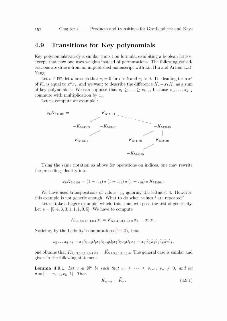
Chapter 4 — Products and transitions for Grothendieck and Keys
4.9 Transitions for Key polynomialsKey polynomials satisfy a similar transition formula, exhibiting a boolean lattice,except that now one uses weights instead of permutations. The following consid-erations are drawn from an unpublished manuscript with Lin Hui and Arthur L.B.Yang.
Let v ∈ Nn, let k be such that vi = 0 for i > k and vk > 0. The leading term xv
of Kv is equal to xuxk, and we want to describe the difference Kv−xkKu as a sumof key polynomials. We can suppose that v1 ≥ · · · ≥ vk−1, because π1, . . . , πk−2
commute with multiplication by xk.Let us compute an example :
x6K543103 = K543104
ooooooo
WWWWWWWWWW
−K544103 −K543401
ooooooo−K543140
ooooooo
K544301 K544130 K543410
ooooooo
−K544310
Using the same notation as above for operations on indices, one may rewritethe preceding identity into
x6K543103 = (1− τ43) ? (1− τ41) ? (1− τ40) ? K543104 .
We have used transpositions of values τ4i, ignoring the leftmost 4. However,this example is not generic enough. What to do when values i are repeated?
Let us take a bigger example, which, this time, will pass the test of genericity.Let v = [5, 4, 3, 3, 1, 1, 1, 0, 5]. We have to compute
K5,4,3,3,1,1,1,0,4 x9 = K5,4,4,3,3,1,1,1,0 π3 . . . π8 x9 .
Noticing, by the Leibnitz’ commutations (1.4.3), that
π3 . . . π8 x9 = x3∂3x4∂4x5∂5x6∂6x7∂7x8∂8 x9 = x3 π3π4π5π6π7π8 ,
one obtains that K5,4,3,3,1,1,1,0,4 x9 = K5,4,3,3,1,1,1,0,4. The general case is similar andgiven in the following statement.
Lemma 4.9.1. Let v ∈ Nn be such that v1 ≥ · · · ≥ vn−1, vn 6= 0, and letu = [. . . , vn−1, vn−1]. Then
Ku xn = Kv . (4.9.1)
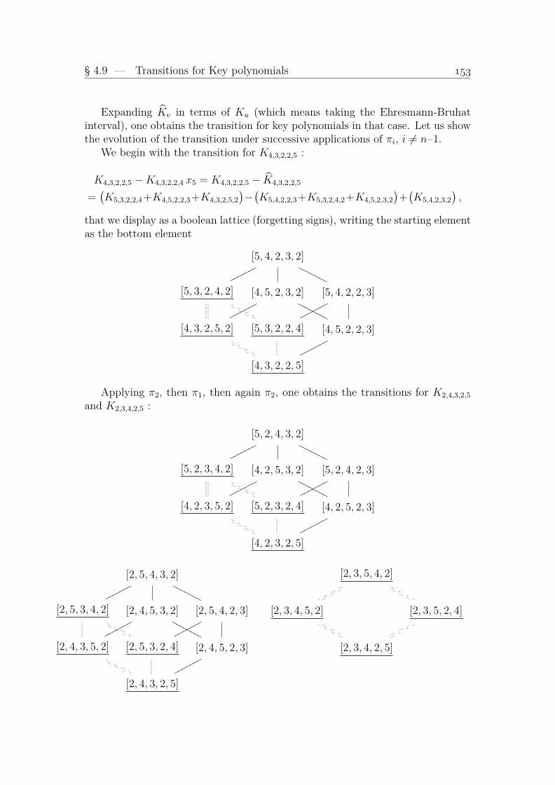
§ 4.9 — Transitions for Key polynomials
Expanding Kv in terms of Ku (which means taking the Ehresmann-Bruhatinterval), one obtains the transition for key polynomials in that case. Let us showthe evolution of the transition under successive applications of πi, i 6= n−1.
We begin with the transition for K4,3,2,2,5 :
K4,3,2,2,5 −K4,3,2,2,4 x5 = K4,3,2,2,5 − K4,3,2,2,5
=(K5,3,2,2,4+K4,5,2,2,3+K4,3,2,5,2
)−(K5,4,2,2,3+K5,3,2,4,2+K4,5,2,3,2
)+(K5,4,2,3,2
),
that we display as a boolean lattice (forgetting signs), writing the starting elementas the bottom element
[5, 4, 2, 3, 2]
oooooooOOOOOOO
[5, 3, 2, 4, 2] [4, 5, 2, 3, 2]
pppppppNNNNNNNN[5, 4, 2, 2, 3]
ppppppp
[4, 3, 2, 5, 2] [5, 3, 2, 2, 4] [4, 5, 2, 2, 3]
ppppppp
[4, 3, 2, 2, 5]
Applying π2, then π1, then again π2, one obtains the transitions for K2,4,3,2,5
and K2,3,4,2,5 :
[5, 2, 4, 3, 2]
oooooooOOOOOOO
[5, 2, 3, 4, 2] [4, 2, 5, 3, 2]
pppppppNNNNNNNN[5, 2, 4, 2, 3]
ppppppp
[4, 2, 3, 5, 2] [5, 2, 3, 2, 4] [4, 2, 5, 2, 3]
ppppppp
[4, 2, 3, 2, 5]
[2, 5, 4, 3, 2]
pppppppNNNNNNN
[2, 5, 3, 4, 2] [2, 4, 5, 3, 2]
pppppppNNNNNNNN[2, 5, 4, 2, 3]
ppppppp
[2, 4, 3, 5, 2] [2, 5, 3, 2, 4] [2, 4, 5, 2, 3]
ppppppp
[2, 4, 3, 2, 5]
[2, 3, 5, 4, 2]
[2, 3, 4, 5, 2] [2, 3, 5, 2, 4]
[2, 3, 4, 2, 5]

Chapter 4 — Products and transitions for Grothendieck and Keys
The terms which are not underlined cancel two by two at the last stage, because(K•ji•• −K•ji••)π2 = 0.
To write the general transition, we need to introduce, for each pair of integersi, j, an operator τi,j on linear combinations of Ku, defined4 by
K...ui...uj ... ? τi,j = K...uj ...ui... .
Then, one has the following transition formula, similar to the one for Grothendieckpolynomials.
Theorem 4.9.2. Let v ∈ Nn, such that vn > 0, and u = [v1, . . . , vn−1, vn−1]. Leti1 < · · · < ir < n be the places i such that vi is strictly maximal among the valuesvj : i ≤ j < n, vj < vn. Then
Ku xn = Kv ? (1− τi1n) · · · (1− τirn) . (4.9.2)
Proof. When v1 ≥ · · · ≥ vn−1, the statement comes from rewriting the expansionof Kv in (4.9.1) in terms of the operators τin.
Given any k such that vk > vk+1, one has Ku xn πk = Kusk xn. On the otherhand, the product of the RHS of (4.9.2) is obtained by replacing v by vsk andexchanging k and k+1 in the indices of the operators τi,n, except one has thedouble factor (1− τk,n)(1− τk+1,n). In that case the factor (1− τk,n) disappears,and this corresponds to the pairs Kw −Kwsk which vanish under πk. QED
The four examples above must be rewritten
K43224 x5 = K43225 ? (1− τ15)(1− τ25)(1− τ45)
K42324 x5 = K43224 x5 π2 = K42325 ? (1− τ15)(1− τ35)(1− τ45)
K24324 x5 = K42324 x5 π1 = K24325 ? (1− τ25)(1− τ35)(1− τ45)
K23424 x5 = K42324 x5 π2 = K23425 ? (1− τ35)(1− τ45) .
If v ∈ Nn is a vexillary code such that vn 6= 0 and there exists i : vi < vn, thenYv(x,0) and Kv satisfy the same transition :
Yv(x,0) = xkYv′(x,0) + Yu(x,0) & Kv = xkKv′ +Ku ,
with v′ and u vexillary (cf. [124, Lemma 3.10]). Therefore, one has the followingproperty, which is a special case of the expansion of a Schubert polynomial interms of keys given in (7.3.2).
Lemma 4.9.3. If v is a vexillary code, then
Yv(x,0) = Kv . (4.9.3)
For example, there are 23 Schubert polynomials Yv(x,0), v ≤ [3, 2, 1, 0], whichcoincide with the key polynomial of the same index, while Y1010(x,0) = x1(x1+x2+x3)is different from K1010 = x1(x2+x3).
4If needed, u is transformed into u, 0, 0, . . .

§ 4.10 — Vexillary polynomials
4.10 Vexillary polynomialsWe have already stated that vexillary Schubert and key polynomials have a deter-minantal expression. This property is also satisfied by Grothendieck polynomials,and we collect together these three families in the next theorem.
First, dominant polynomials can be written as multi-Schur functions. Let vbe dominant, u = vω, k = v1. Then
Yv = Su(xn − yvn , . . . ,x1 − yv1)
Gv = (x1 · · ·xn)−kSkn(xn − yvn , . . . ,x1 − yv1)
Kv = Su(xn, . . . , x1)
For example, for v = [6, 3, 1], one has
Y631 = S136(x3−y1,x2−y3,x1−y6) =
∣∣∣∣∣∣S1(x3 − y1) S4(x2 − y3) S8(x1 − y6)S0(x3 − y1) S3(x2 − y3) S7(x1 − y6)
0 S2(x2 − y3) S6(x1 − y6)
∣∣∣∣∣∣ ,G631 = (x1x2x3)−6S666(x3 − y1,x2 − y3,x1 − y6) ,
K631 = S136(x3,x2,x1) .
As we already saw, the action of ∂i or πi on a determinant of complete functionsSk(xp−yq) is straightforward if only one column or one row is not invariant underthe transposition of xi, xi+1. In that case, one has to transform this row or column,following the rules Sk(xi − y)∂i = Sk−1(xi+1 − y), Sk(xi − y)πi = Sk(xi+1 − y).
For example,
Y631∂2−−→Y612 = S126(x3 − y1,x3 − y3,x1 − y6)
∂1−−→Y152
= S125(x3 − y1,x3 − y3,x2 − y6)∂2−−→Y124 = S124(x3 − y1,x3 − y3,x3 − y6) ,
G631(x1x2x3)6 π2−−→ = S666(x3 − y1,x3 − y3,x1 − y6)π1−−→
= S666(x3 − y1,x3 − y3,x2 − y6)π2−−→ = S666(x3 − y1,x3 − y3,x3 − y6) .
On the other hand, Y631∂1 = S135(x3 − y1,x2 − y3,x2 − y6) and we cannotproceed so easily with ∂2, since two columns involve x2 and not x3.
When v is vexillary, we have already used the property that there exists atleast one sequence of operators ∂i or πi respectively, starting from a dominantcase, such that at each step, only one column is transformed by the operator
To describe the missing determinants in the Grothendieck case, we have tofollow the same recursion than for Schubert, but with different flags. To anyv ∈ Nn, let us associate the two following flags of alphabets. Let w be thesequence wi := max(j : j ≥ i, vj ≥ vi. Then vx is the decreasing reordering of w.Let now u be the element of Nn obtained by decreasingly reordering v accordingto the rule [. . . i, j . . .] → [. . . j+1, i . . .] whenever i < j. Then vy is set to be theincreasing reordering of u.

Chapter 4 — Products and transitions for Grothendieck and Keys
Theorem 4.10.1. Let v ∈ Nn be vexillary, vx, vy be the two vectors defined above,k = max(vy). Then
Yv = Sv↑(xvx1 − yvy1 , . . . ,xvxn − yvyn) , (4.10.1)Gv = Skn(xvx1 − yvy1 , . . . ,xvxn − yvyn) (x1 · · ·xn)−k , (4.10.2)Kv = Sv↑(xvx1 , . . . ,xvxn) . (4.10.3)
In particular, when v is vexillary, then Kv = Yv(x,0).
For example, for v = [3, 5, 4, 0, 2], one has w = [3, 2, 3, 5, 5], which reorders intovx = [5, 5, 3, 3, 2]. On the other hand, the chain v = [3, 5, 4, 0, 2]→ [6, 3, 4, 0, 2]→[6, 5, 3, 0, 2]→ [6, 5, 3, 3, 0] gives the second flag vy = [0, 3, 3, 5, 6]. Hence, one has
Y35402 = S02345(x5−y0,x5−y3,x3−y3,x3−y5,x2−y6)
G35402 = S66666(x5−y0,x5−y3,x3−y3,x3−y5,x2−y6)(x1 . . . x5)−6
K35402 = S02345(x5,x5,x3,x3,x2) .
Property (2.6.5) allows to write from (4.10.2) a determinantal formula for Gv
polynomials such that v♣ be vexillary. This condition is in fact equivalent torequiring that v be vexillary, since if a permutation σ avoids the pattern 2143,then ωσω also avoids this pattern, and conversely.
§ 4.11 — Grothendieck and Yang-Baxter
4.11 Grothendieck and Yang-BaxterOne can degenerate Yang-Baxter bases of Hecke algebras into bases of the 0-Hecke algebra, i.e. the algebra generated by π1, π2, . . . . But as in the case ofdivided differences, instead of taking products of factors of the type πi+1/c, let ustake factors 1 + cπi. Accordingly, given a spectral vector [y1, . . . , yn], one definesrecursively a Yang-Baxter basis fbπ
σ, starting from 1 for the identity permutation,by
fbπσsi
= fbπσ
(1 +
(1− yσi
yσi+1
)πi
)for σi < σi+1 . (4.11.1)
For example,
fbπ321 =
(1 +
(1− y1
y2
)π1
)(1 +
(1− y1
y3
)π2
)(1 +
(1− y2
y3
)π1
)= 1 +
(1− y1
y3
)π1 +
(1− y1
y3
)π2 +
(1− y1
y2
)(1− y1
y3
)π1π2
+
(1− y2
y3
)(1− y1
y3
)π2π1 +
(1− y1
y2
)(1− y1
y3
)(1− y2
y3
)π1π2π1 .
s As in the case of divided differences, the Yang-Baxter coefficients are speciali-sations of known polynomials. The proof of the next properties is similar to theproof of Theorem 3.5.1, and we can avoid repeating it.
Theorem 4.11.1. The matrix of change of basis between fbπσ and πσ, and its
inverse, have entries which are specializations of Grothendieck polynomials :
fbπσ =
∑ν≤σ
πν G(ν)(yσ,y) , (4.11.2)
πν∏i<j
(1− yi
yj
)=
∑σ≤ν
(−1)`(σ)−`(ν)fbπσ G(ν−1ω)(y
ω,yσ) . (4.11.3)
For example, for ν = [2, 3, 1], one has ν−1ω = [2, 1, 3], and the coefficients ofthe expansion of π231 are specialisations of the polynomial G(213 = 1−y1x
−11 . One
has
π231
∏i<j≤3
(1− yiy−1j ) = fbπ
123G(213(y321,y)− fbπ213G(213(y321,y213)
− fbπ132G(213(y321,y132) + fbπ
231G(213(y321,y231)
=
(1− y1
y3
)fbπ
123 −(
1− y2
y3
)fbπ
213 −(
1− y1
y3
)fbπ
132 +
(1− y2
y3
)fbπ
231 .
The general properties of Yang-Baxter bases induce properties of specializa-tions of Grothendieck polynomials.

Chapter 4 — Products and transitions for Grothendieck and Keys
The symmetry (1.8.4) entails(G(ν)(y
σ,y))♣
= G(ωνω)(yωσω,yω) , (4.11.4)
using the involution ♣ : yi → y−1n+1−i, i = 1, . . . , n introduced in (2.6.4).
Each of the equations (1.8.9) and (1.8.10) gives, after some rewriting,∑ν
(−1)`(ν)+`(σ)G(ν)(yσ,y)G(νω)(y
ζ ,y) = δσ,ζω∏i<j
(1− yi
yj
), (4.11.5)
which is a special instance of formula (2.9.4).

Chapter 5G1/x and G Grothendieck polynomials
In the preceding sections, we have seen that Grothendieck and Schubert polynomi-als satisfy similar properties. To relate these two families precisely, it is convenientto perform a change of variables in the former. In fact, we shall use two slightlydifferent transformations, in view of different geometrical considerations.
5.1 Grothendieck in terms of SchubertDenote the image of the Grothendieck polynomial Gv(x,y) under the inversionxi → x−1
i , yi → yi, by G1/xv (x,y), and by Gv(x,y) the image under the transfor-
mation1
xi → (1− xi)−1 , yi → (1− yi)−1, i = 1, 2, . . .
Thus, in the dominant case, for λ ∈ Nn a partition, one has
G1/xλ (x,y) =
n∏i=1
λi∏j=1
(yj−xi)y−1j & Gλ(x,y) =
n∏i=1
λi∏j=1
(xi−yj)(1−yj)−1 ,
and the other polynomials are generated using respectively the operators
π1/xi = −xi+1∂i & πi = (1− xi+1) ∂i , (5.1.1)
or the generation in y seen in (2.2.3), which uses the isobaric divided differencesin y in the first case, or in the indeterminates y1−1, y2−1, . . . in the second case :
πyi & πy−
i = (yi − 1)∂yi . (5.1.2)
1 Many authors use the transformation xi → (1− xi)−1, yi → (1− yi). This not compatiblewith simultaneously using Yv(x,y), but only with Yv(x,0). In fact, the factor x+y−xy, insteadof 1−x/y) or (x− y)/1−y) that we now take, does not possess the right symmetry in x, y whichis imposed by geometry.
159

Chapter 5 — G1/x and G Grothendieck polynomials
For example, the polynomial G1/x01 (x,y) = 1 − x1x2y
−11 y−1
2 is the image ofG
1/x20 (x,y) = (1−x1y
−11 )(1−x1y
−12 ) under π1/x
1 = −x2∂1, as well as the image ofG
1/x11 (x,y) = (1−x1y
−11 )(1−x2y
−11 ) under πy
1 .From the expression of πi, one sees that the basis Gv(x,y) is triangular in the
basis Yv(x,y), the term of Gv(x,y) of lowest degree being
(1− y1)−u1(1− y2)−u2 · · ·Yv(x,y) ,
with u the code of the permutation inverse to 〈v〉.Any example reveals that the expansion of these new polynomials in the
Schubert basis posseses a structure quite willing to uncover itself. For exam-ple, v = [2, 0, 2, 1] is the code of the permutation [3, 1, 5, 4, 2], the code of theinverse permutation is equal to u = [1, 3, 0, 1, 0], and one has
(1−y1)(1−y2)3(1−y4)G2021 = Y2021
kkkkkkkkkkkkk
TTTTTTTTTTTT
1y1−1
Y2220
RRRRRRRRRR
1y3−1
Y3021
llllllllll
SSSSSSSSSS
y1+y2−2(y1−1)2
Y2121
kkkkkkkkk
1(y1−1)(y3−1)
Y3220
RRRRRRRR
1(y1−1)2
Y2221y1+y2−2
(y1−1)2(y3−1)Y3121
kkkkkkkk
1(y1−1)2(y3−1)
Y3221
A similar computation gives the expansion ofG1/x2021(x,y) (writing Yv for Yv(x,y)) :
G1/x2021(x,y) = − 1
y1y23y4
Y2021 −(y1 + y2)
y13y2
3y4
Y2121 −1
y12y2
3y4
Y222
− 1
y13y2
3y4
Y2221 −1
y1y23y3y4
Y3021 −(y1 + y2)
y13y2
3y3y4
Y3121
− 1
y12y2
3y3y4
Y322 −1
y13y2
3y3y4
Y3221 .
On this single example, it appears that the two expansions are identical, up to aminor transformation of coefficients. Indeed, since a Schubert polynomial Yv(x,y)is invariant under a uniform translation xi → xi + ε, yi → yi + ε, i = 1, 2, . . . , theexpansion of Gv(x,y) is obtained from the expansion of G1/x(x,y) by the changeof variables yi → yi−1 in the coefficients.
Notice however that the polynomials in x only are different. In the case ofG
1/xv (x,y), one has to specialize y to 1, 1, . . . , while for Gv(x,y), one sends y
to 0, 0, . . . . Thus G1/x01 (x,y) = −y−1
2 Y01(x,y)− y−11 y−1
2 Y11(x,y) gives
G1/x01 (x,1) = −Y01(x,1)− Y11(x,1) = 1− x1x2

§ 5.1 — Grothendieck in terms of Schubert
while G01(x,y) = (1−y2)−1Y01(x,y)− (1−y1)−1(1−y2)−1Y11(x,y) induces
G01(x,0) = Y01(x,0)− Y11(x,0) = x1 + x2 − x1x2 .
Normalizing for a moment the polynomials in such a way that ˜Gv = Yv + . . . ,one renders the matrix of change of basis unitriangular. Here it is, together with itsinverse, for n = 4, putting A = (y1−1)−1, B = (y2−1)−1, C = (y1 +y2−2)(1−y1)−2.
000
001
010
100
020
011
200
101
110
300
021
201
120
111
210
301
220
310
121
211
320
311
221
321
1 · · · · · · · · · · · · · · · · · · · · · · ·· 1 · · · B · · · · · · · AB · · · · · · · · · ·· · 1 · · · · · A · · · · · · · · · · · · · · ·· · · 1 · · · · · · · · · · · · · · · · · · · ·· · · · 1 · · · · · · · A · · · · · · · · · · ·· · · · · 1 · · · · · · · C · · · · · · · · · ·· · · · · · 1 · · · · · · · · · · · · · · · · ·· · · · · · · 1 · · · B · A · · · · · AB · · · ·· · · · · · · · 1 · · · · · · · · · · · · · · ·· · · · · · · · · 1 · · · · · · · · · · · · · ·
· · · · · · · · · · 1 · · · · · A · C · · · A2 ·· · · · · · · · · · · 1 · · · · · · · A · · · ·· · · · · · · · · · · · 1 · · · B · · · · · · ·· · · · · · · · · · · · · 1 · · · · · · · · · ·· · · · · · · · · · · · · · 1 · · · · · · · · ·· · · · · · · · · · · · · · · 1 · · · · · A · ·· · · · · · · · · · · · · · · · 1 · · · · · · ·· · · · · · · · · · · · · · · · · 1 · · · · · ·· · · · · · · · · · · · · · · · · · 1 · · · B ·· · · · · · · · · · · · · · · · · · · 1 · · · ·· · · · · · · · · · · · · · · · · · · · 1 · · ·· · · · · · · · · · · · · · · · · · · · · 1 · ·· · · · · · · · · · · · · · · · · · · · · · 1 ·· · · · · · · · · · · · · · · · · · · · · · · 1
For example, the row of index 101 must be read
˜G101 = (y1 − 1)(y3 − 1)G101
= Y101 +1
y2 − 1Y201 +
1
y1 − 1Y111 +
1
(y2 − 1)(y1 − 1)Y211 ,
or equivalently
y1y3G1/x101 = Y101 + y−1
2 Y201 + y−11 Y111 + y−1
1 y−12 Y211 .
The inverse matrix looks very similar, apart from signs, and different locationof the non-zero entries.

Chapter 5 — G1/x and G Grothendieck polynomials
000
001
010
100
020
011
200
101
110
300
021
201
120
111
210
301
220
310
121
211
320
311
221
321
1 · · · · · · · · · · · · · · · · · · · · · · ·
· 1 · · · −B · · · · · · · A2 · · · · · · · · · ·
· · 1 · · · · · −A · · · · · · · · · · · · · · ·
· · · 1 · · · · · · · · · · · · · · · · · · · ·· · · · 1 · · · · · · · −A · · · AB · · · · · · ·
· · · · · 1 · · · · · · · −C · · · · · · · · · ·
· · · · · · 1 · · · · · · · · · · · · · · · · ·· · · · · · · 1 · · · −B · −A · · · · · · · · · ·
· · · · · · · · 1 · · · · · · · · · · · · · · ·· · · · · · · · · 1 · · · · · · · · · · · · · ·· · · · · · · · · · 1 · · · · · −A · −C · · · AB ·
· · · · · · · · · · · 1 · · · · · · · −A · · · ·
· · · · · · · · · · · · 1 · · · −B · · · · · · ·
· · · · · · · · · · · · · 1 · · · · · · · · · ·· · · · · · · · · · · · · · 1 · · · · · · · · ·· · · · · · · · · · · · · · · 1 · · · · · −A · ·
· · · · · · · · · · · · · · · · 1 · · · · · · ·· · · · · · · · · · · · · · · · · 1 · · · · · ·· · · · · · · · · · · · · · · · · · 1 · · · −B ·
· · · · · · · · · · · · · · · · · · · 1 · · · ·· · · · · · · · · · · · · · · · · · · · 1 · · ·· · · · · · · · · · · · · · · · · · · · · 1 · ·· · · · · · · · · · · · · · · · · · · · · · 1 ·· · · · · · · · · · · · · · · · · · · · · · · 1
For example, the row of index 021 must be read, with the normalized polyno-
mials ˜Gv, or the polynomials G1/xv ,
Y021 =˜G021 +
1
1−y1
˜G22 +
(1
1−y1
+1−y2
(1−y1)2
) ˜G121 +
1
(1−y1)(1−y2)˜G221
Y021 = −y22y3G
1/x021 − y1y2
2G1/x22 − y1y3 (y1 + y2)G
1/x121 − y1
2y2G1/x221 .
Let us precise and prove the observation of the closeness between the twomatrices. Thanks to (2.6.5), the orthogonality relation between the polynomialsGv and Gu can be rewritten as
(Guxρ)ω y−ρGv πω ∈ ±1, 0 . (5.1.3)
Since the operator xρω πω is equal to
(x1 . . . xn)n−1∂ω =(∑
(−1)`(σ)σ)
(x1 . . . xn)n−1∆(x)−1
its image under the change of variables xi → (1−xi)−1 is the operator(∑
(−1)`(σ)σ)
∆(x)−1 = ∂ω .
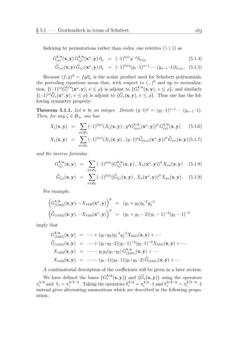
§ 5.1 — Grothendieck in terms of Schubert
Indexing by permutations rather than codes, one rewrites (5.1.3) as
G1/x(σ) (x,y)G
1/x(ζ) (xω,y) ∂ω = (−1)`(σ)y−ρδσ,ζω (5.1.4)
G(σ)(x,y) G(ζ)(xω,y) ∂ω = (−1)`(σ)(y1−1)n−1 · · · (yn−1−1)δσ,ζω . (5.1.5)
Because (f, g)∂ = fg∂ω is the scalar product used for Schubert polynomials,the preceding equations mean that, with respect to ( , )∂ and up to normaliza-tion, (−1)|v|G
1/xv (xω,y), v ≤ ρ is adjoint to G1/x
v (x,y), v ≤ ρ, and similarly(−1)|v|Gv(x
ω,y), v ≤ ρ is adjoint to Gv(x,y), v ≤ ρ. Thus one has the fol-lowing symmetry property:
Theorem 5.1.1. Let n be an integer. Denote (y−1)ρ = (y1−1)n−1 · · · (yn−1−1).Then, for any ζ ∈ Sn, one has
Xζ(x,y) =∑σ∈Sn
(−1)`(σ)(Xζ(x,y) , yρG1/x(σω)(x
ω,y))∂ G1/x(σ) (x,y) (5.1.6)
Xζ(x,y) =∑σ∈Sn
(−1)`(σ)(Xζ(x,y) , (y−1)ρG(σω)(xω,y))∂ G(σ)(x,y)(5.1.7)
and the inverse formulas
G1/x(ζ) (x,y) =
∑σ∈Sn
(−1)`(σ)(G1/x(ζ) (x,y) , Xσ(xω,y))∂ Xσω(x,y) (5.1.8)
G(ζ)(x,y) =∑σ∈Sn
(−1)`(σ)(G(ζ)(x,y) , Xσ(xω,y))∂ Xσω(x,y) . (5.1.9)
For example,(G
1/x(1342)(x,y),−X1432(xω,y)
)∂= (y1 + y2)y−2
1 y−22(
G(1342)(x,y),−X1432(xω,y))∂
= (y1 + y2 − 2)(y1 − 1)−2(y2 − 1)−2
imply that
G1/x(1342)(x,y) = · · ·+ (y1+y2)y−2
1 y−22 X2341(x,y) + · · ·
G(1342)(x,y) = · · ·+ (y1+y2−2)(y1−1)−2(y2−1)−2X2341(x,y) + · · ·X1432(x,y) = · · · − y1y3(y1+y2)G
1/x(2431)(x,y) + · · ·
X1432(x,y) = · · · − (y1−1)(y3−1)(y1+y2−2) G(2431)(x,y) + · · ·
A combinatorial description of the coefficients will be given in a later section.We have defined the bases G1/x
v (x,y) and Gv(x,y) using the operatorsπ
1/xi and πi = π
1/1−xi . Taking the operators π1/x
i = π1/xi−1 and π1/1−x
i = π1/1−xi
−1instead gives alternating summations which are described in the following propo-sition.

Chapter 5 — G1/x and G Grothendieck polynomials
Proposition 5.1.2. Given n, σ ∈ Sn, one has the following identities involvingthe Ehresmann-Bruhat interval [σ, ω], and the alphabets 1−x = 1−x1, 1−x2, . . . and 1−y = 1−y1, 1−y2, . . . .
xρ∑ζ≤σ
(−1)`(ζ)G(ζ)(x,y) = yρG1/xσ (x,y) (5.1.10)
(1−x)−ρ∑ζ≤σ
(−1)`(ζ)G(ζ)(x,y) = (1−y)ρG1/xσ (1−x,1−y) (5.1.11)
x−ρ∑ζ≤σ
(−1)`(ζ)G1/x(ζ) (x,y) = y−ρGσ(x,y) . (5.1.12)
Proof. The three identities result from each other by change of variables, let usconsider the first one. Its left-hand side can be written (−1)`(σ)Gω(x,y)π(ωσ)(x,y).However, π1/x
i x−ρ = −xi+1∂ix−ρ = −x−ρπi. Therefore
(−1)`(σ)Gω(x,y)π(ωσ)(x,y) = (−1)`(ω)G1/xω (x,y)x−ρyρπωσ
= G1/xω (x,y)π1/x
ωσ yρ = G1/x
σ (x,y)yρ ,
which is the required identity. QEDCombining 5.1.10 and 2.6.5, one can also express the adjoint basis Gv(x,y)
with alternating summations:∑ζ≤σ
(−1)`(ζ)G1/x(ζ) (x,y) = G(ωσω)(x
ω,y) . (5.1.13)
For example, for σ = [1, 3, 2], one has
G1/x01 (x,y)−G
1/x11 (x,y)−G
1/x20 (x,y)+G
1/x21 (x,y)
= 1−x2x1
y1y2
−(
1−x1
y1
)(1−x2
y1
)−(
1−x1
y1
)(1−x1
y2
)+
(1−x1
y1
)(1−x1
y2
)(1−x2
y1
)=x1 (x2x1 − y1y2)
y12y2
= G(213)(xω,y) .
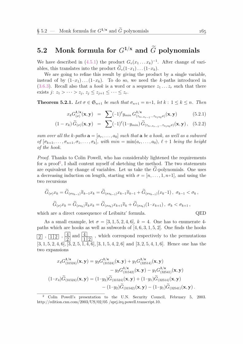
§ 5.2 — Monk formula for G1/x and G polynomials
5.2 Monk formula for G1/x and G polynomialsWe have described in (4.5.1) the product Gv(x1 . . . xk)
−1. After change of vari-ables, this translates into the product Gv(1−x1) . . . (1−xk).
We are going to refine this result by giving the product by a single variable,instead of by (1−x1) . . . (1−xk). To do so, we need the k-paths introduced in(3.6.3). Recall also that a hook is a word or a sequence z1 . . . zr such that thereexists j: z1 > · · · > zj, zj ≤ zj+1 ≤ · · · ≤ zr.
Theorem 5.2.1. Let σ ∈ Sn+1 be such that σn+1 = n+1, let k : 1 ≤ k ≤ n. Then
xkG1/x(σ) (x,y) =
∑(−1)`yminG
1/x(τar,ar−1 ...τa1a0σ)(x,y) (5.2.1)
(1− xk) G(σ)(x,y) =∑
(−1)`(1−ymin) G(τar,ar−1 ...τa1a0σ)(x,y) , (5.2.2)
sum over all the k-paths a = [ar, . . . , a0] such that a be a hook, as well as a subwordof [σk+1, . . . , σn+1, σ1, . . . , σk], with min = min(ar, . . . , a0), ` + 1 being the heightof the hook.
Proof. Thanks to Colin Powell, who has considerably lightened the requirementsfor a proof2, I shall content myself of sketching the method. The two statementsare equivalent by change of variables. Let us take the G-polynomials. One usesa decreasing induction on length, starting with σ = [n, . . . , 1, n+1], and using thetwo recursions
G(σ)xk = G(σsk−1)πk−1xk = G(σsk−1)xk−1πk−1 + G(σsk−1)(xk−1) , σk−1 < σk ,
G(σ)xk = G(σsk)πkxk = G(σsk)xk+1πk + G(σsk)(1−xk+1) , σk < σk+1 ,
which are a direct consequence of Leibnitz’ formula. QED
As a small example, let σ = [3, 1, 5, 2, 4, 6], k = 4. One has to enumerate 4-paths which are hooks as well as subwords of [4, 6, 3, 1, 5, 2]. One finds the hooks
2 , 1 2 , 42
and 41 2
, which correspond respectively to the permutations[3, 1, 5, 2, 4, 6], [3, 2, 5, 1, 4, 6], [3, 1, 5, 4, 2, 6] and [3, 2, 5, 4, 1, 6]. Hence one has thetwo expansions
x4G1/x(31524)(x,y) = y2G
1/x(31524)(x,y) + y1G
1/x(32514)(x,y)
− y2G1/x(31542)(x,y)− y1G
1/x(32541)(x,y)
(1−x4)G(31524)(x,y) = (1−y2)G(31524)(x,y) + (1−y1)G(32514)(x,y)
− (1−y2)G(31542)(x,y)− (1−y1)G(32541)(x,y) .
2 Colin Powell’s presentation to the U.N. Security Council, February 5, 2003.http://edition.cnn.com/2003/US/02/05 /sprj.irq.powell.transcript.10.

Chapter 5 — G1/x and G Grothendieck polynomials
Let us illustrate the recursion for Monk formula on a bigger example. Letk = 4, σ = [1, 3, 4, 6, 2, 7, 5, 8] (resp. σ = [1, 3, 4, 6, 2, 5, 7, 8]).
Suppressing the terminal 8 which is a fixed point of all the permutations in-volved, one has
(1−x4)G(1346275) = (1−y6)G(1346275) − (1−y6)G(1347265) + (1−y4)G(1364275)
−(1−y4)G(1365274)+(1−y3)G(1463275)−(1−y4)G(1367245)+(1−y4)G(1367254)−(1−y3)G(1465273)
+ (1−y1)G(3461275) − (1−y3)G(1467235) + (1−y3)G(1467253) − (1−y1)G(3462175) ,
(1−x4)G(1346257) = (1−y6)G(1346257)−(1−y6)G(1347256)+(1−y4)G(1364257)−(1−y4)G(1365247)
+ (1−y3)G(1463257) − (1−y3)G(1465237) + (1−y1)G(3461257) − (1−y1)G(3462157) .
The following two trees describe the cycles ζσ−1 in the preceding expansions(1−x4)Gσ(x,0) =
∑±Gζ(x,0), these cycles being hooks which are subwords of
[2, 7, 5, 1, 3, 4, 6] when σ = [1, 3, 4, 6, 2, 7, 5], and subwords of [2, 5, 7, 1, 3, 4, 6] whenσ = [1, 3, 4, 6, 2, 5, 7].
6
4 6
||||||||??????
??????
76
3 4 6
????????
NNNNNNNNNNNNNN
NNNNNNNNNNNNNN
54 6
LLLLLLLLLLLLLLL
LLLLLLLLLLLLLLL74 6
1 3 4 6 53 4 6
73 4 6
754 6
21 3 4 6
753 4 6
6
4 6
||||||||
76
3 4 6
CCCCCC
54 6
1 3 4 6 53 4 6
21 3 4 6
For example, the two bottom elements of the left tree must be read as follows.
The two permutations σ=13462753462175
differ by the cycle (1 → 3 → 4 → 6 → 2),
that one writes as a hook finishing by 6:21 3 4 6 . The minimum of the cycle
is 1, the height of the hook is 2, and therefore the corresponding term in thedecomposition of (1−x4)G(sigma)(x,y) is −(1−y1)G(3462175)(x,y).
Similarly, σ=13462751467253
differ by the cycle (3 → 4 → 6 → 7 → 5), that one

§ 5.2 — Monk formula for G1/x and G polynomials
writes753 4 6
. The minimum of the cycle is 3, the height of the hook is 3, hence
the term (1−y3)G(1467253)(x,y).
Lenart[138, Th.3.1] describes the product xkGv(x,0) in terms of chains in the“k-Bruhat order” and criticizes (4.5.1) for involving cancellations. For our defense,we shall put forward that this is not the same case which is treated in the twoformulas. In the former, one multiplies by 1−xk, in the later, taking into accountthe change of variables, by (1−x1) . . . (1− xk).
The Pieri formula for the products Gv(x,0)G0i,1j(x,0) or Gv(x,0)G0i,j(x,0)is given by Lenart and Sottile [140].

Chapter 5 — G1/x and G Grothendieck polynomials
5.3 Transition for G1/x and G polynomialsBy change of variables, one transforms (4.7.2) into a transition formula for G1/x
and Gpolynomials.
Proposition 5.3.1. Let v ∈ Nk be such that vk > 0, let σ be the permutation ofcode v′ = [v1, . . . , vk−1, vk−1]. Then, with the conventions of (4.7.2), one has(
G1/xv′ −G
1/xv
) yjxk
= (1− τjim) ? · · · (1− τji1) ? G1/x(σ) (5.3.1)(
Gv′ − Gv
) 1− yj1− xk
= (1− τjim) ? · · · (1− τji1) ? G(σ) . (5.3.2)
These expressions are not a direct corollary of Monk formula for G-polynomials.For example, for v = [1, 0, 1, 1], one has σ = [2, 1, 4, 3, 5], and, writing at the sametime codes and permutations,(
G1010021435
− G1011021453
) 1−y3
1−x4
= (1− τ32)(1− τ31) ? G1010021435
= G1010021435
− G1110023415
− G2010031425
+ G2110032415
,
while, writing also in a box the hooks appearing in the statement of (5.2.2), onehas the Monk formula
(1−x4)G1010021435
= (1−y3)G1010021435
3 + (1−y1)G1110023415
13 + (1−y2)G2010031425
23
− (1−y3)G1011021453
53 − (1−y1)G11110
23451
513 − (1−y2)G20110
31452
523 .

§ 5.4 — Action of divided differences on G1/x and G polynomials
5.4 Action of divided differences on G1/x and G
polynomialsLet us show that the property that, up to normalization, G1/x
v (xω,y), v ≤ ρis adjoint to G1/x
v (x,y), v ≤ ρ, and similarly Gv(xω,y), v ≤ ρ is adjoint to
Gv(x,y), v ≤ ρ, allows to exchange multiplication by xi with ∂n−i.
Indeed, for any σ, ζ ∈ Sn, any i ≤ n−1, let ζ ′ = ζsi if ζi ≥ ζi+1 or or ζ ′ = ζ
otherwise. Consequently, G1/xζ (x,y)(−xi+1∂i) = G
1/xζ′ (x,y).
Then, according to Theorem 5.1.1, one has
yρ(−1)`(σ)δζ′,ωσ =((G
1/x(ζ) (x,y)(−xi+1∂i)
)ω, G
1/x(σ) (x,y)
)∂=(−(G
1/x(ζ) (x,y)xi+1
)ωω∂iω,G
1/x(σ) (x,y)
)∂=((G
1/x(ζ) (x,y)xi+1
)ω, G
1/x(σ) (x,y)∂n−i
)∂.
Therefore, up to reversal of alphabets, multiplication and divided differencesare exchanged. Thus, let a ¬ hook be a word z1 . . . zr such that there exists j:z1 ≤ · · · ≤ zj, zj > zj+1 > · · · > zr. Then Monk formulas (5.2.1) and (5.2.2)translate about the following description of the action of divided differences.
Theorem 5.4.1. Let σ ∈ Sn, k : 1 ≤ k ≤ n−1 be such that σk > σk+1, andη = σsk. Then
G1/x(σ) (x,y)∂k =
∑(−1)` y−1
maxG1/x(τar,ar−1 ...τa1a0η)(x,y) (5.4.1)
G(σ)(x,y)∂k =∑
(−1)`−1(1−ymax)−1G(τar,ar−1 ...τa1a0η)(x,y) , (5.4.2)
sum over all the k-paths a = [ar, . . . , a0] such that a be a ¬ hook, as well as asubword of [ηk+1, . . . , ηn+1, η1, . . . , ηk], with max = max(ar, . . . , a0), ` being thewidth of the ¬ hook.
For example, for k = 3, σ = [3, 1, 5, 2, 6, 4], then η = [3, 1, 2, 5, 6, 4], and,writing each polynomial together with its ¬ hook, one has
G1/x(3,1,5,2,6,4) ∂3 = − 2 y−1
2 G1/x(3,1,2,5,6,4) − 4
2y−1
4 G1/x(3,1,4,5,6,2)
+ 1 2 y−12 G
1/x(3,2,1,5,6,4) + 1 4
2y−1
4 G1/x(3,4,1,5,6,2)
+ 3 42y−1
4 G1/x(4,1,3,5,6,2) − 1 3 4
2y−1
4 G1/x(4,3,1,5,6,2) ,

Chapter 5 — G1/x and G Grothendieck polynomials
G(3,1,5,2,6,4)∂3 = 21
1− y2
G(3,1,2,5,6,4) + 42
1
1− y4
G(3,1,4,5,6,2)
− 1 21
1− y2
G(3,2,1,5,6,4) − 1 42
1
1− y4
G(3,4,1,5,6,2)
− 3 42
1
1− y4
G(4,1,3,5,6,2) + 1 3 42
1
1− y4
G(4,3,1,5,6,2) .

§ 5.5 — Still more keys: KG polynomials
5.5 Still more keys: KG polynomialsWhen σ is Grassmannian, Xσ(x,0) is equal to a Schur function, as well as to akey polynomial. The polynomial G(σ)(x,0) is also symmetrical, but not equal toa Schur function, nor to any classical symmetric function. 0ne has to find anotherfamily of polynomials which play the role of key polynomials versus Schubert poly-nomials, and coincide with the polynomials G(σ)(x,0) in the symmetric case. Thepolynomials KG
v seen in (4.6.2) play such a role with respect to G(σ)(x,1). There-fore, we define the polynomials KG
v , v ∈ Nn, to be the images of the polynomialsKGv under the transformation xi → (1−xi)
−1. In fact, these are the polynomialsdenoted KG[v] in [104].
The corresponding operators are
Di = xi(1− xi+1) ∂i = (1− xi+1) πi ,
which can be characterized by
1Di = 1 & xi+1(1− xi+1)−1 Di = 0
and, therefore, are obtained from the isobaric divided differences by the change ofvariable xi → xi(1−xi)
−1. In short, Di = πx/(1−x)i .
In explicit terms,
KGλ = xλ when λ dominant & KG
vsi= KG
v Di when vi ≥ vi+1 . (5.5.1)
For example, for the weights which are permutations of [4, 2, 0] these key poly-nomials expand in the usual key polynomials as follows :
KG420 = K42
KG402 = K402 −K412
KG240 = K24 −K34
KG204 = K204 −K214 −K304 +K314
KG042 = K042 +K242 − 2K142 +K341 −K34
KG024 = K024 −K234 + 2K134 −K034 +K224 − 2K124
Notice that the image of πω = xρ∂ω under the change of variables is
Dω = xn−11 . . . xn−1 (1−x2) . . . (1−xn)n−1 ∂ω = (1−x2) . . . (1−xn)n−1 πω , (5.5.2)
so that
KGλω = xλ(1−x2) · · · (1−xn)n−1 πω = xλ+ρ(1−x2) · · · ∂ω = Gλω(x,0) . (5.5.3)
The following proposition is the image of Proposition 4.6.1 by the transforma-tion xi → (1−xi)
−1 and shows how to generate the polynomials Gv(x,0) using theoperators Di.

Chapter 5 — G1/x and G Grothendieck polynomials
Proposition 5.5.1. Given v ∈ Nn, let k be such that vk = 0 and vi > 0 fori < k. (if no component of v is 0, change n → n+1, v → [v, 0]). Let u =[v1 − 1, . . . , vk−1 − 1, vk+1, . . . , vn]. Then
Gv(x,0) = Gu(x,0) (xk−1 · · ·x1) Dn−1 · · · Dk
= Gu(x,0) Dn−1 · · · Dk (xk−1 · · ·x1) . (5.5.4)
For example, if v = [3, 0, 4], then k = 2, u = [3−1, 4], and
G304(x,0) = G24(x,0)x1D2 = G24(x,0)x1(1−x3) π2 .
As in the case of Schubert polynomials, the preceding proposition can be usedto expand the polynomials Gu(x,0) in terms of the KG
v . For example,
G2042(x,0) = KG2042 + KG
5012 + KG3041 − KG
3042 − KG5022 − KG
5031 + KG5032 ,
the leading terms corresponding to
Y2042(x,0) = K2042 +K5012 +K3041 .
The appropriate quadratic form (which is not symmetric) is
(f, g)G = CT
(f g♣
∏1≤i<j≤n
(1− xi
xj
(1− xj)(1− xi)
))=
(f
1
(1−x1)n−1 . . . (1−xn−1), g
)taking the scalar product ( , ) used for key polynomials, and the involution ♣ :xi → x−1
n+1−i.One checks that, with Di = (xi−1)∂i, one has(
f Di , g)G
=(f , g Dn−i
)G, (5.5.5)
the proof of the statement being reduced, as usual, to the case n = 2.This leads to define still another basis,
KGλ = xλ when λ dominant &
KGvsi
=KGv ∂i(xi+1−1) when vi ≥ vi+1 . (5.5.6)
The rest of this section depends on the following lemma, that we leave as anopen question for lack of a simple proof.
Lemma 5.5.2. For any dominant λ ∈ Nn, any v ∈ Nn, one has(KGv , x
λ)G
= δv,λω . (5.5.7)
The equations (5.5.5) and (5.5.7) give by a recursion that we already usedseveral times a pair of adjoint bases:

§ 5.5 — Still more keys: KG polynomials
Corollary 5.5.3. For u, v ∈ Nn one has(KGv ,
KGu
)G= δv,uω . (5.5.8)
For example,
KG021(1−x1)−2(1−x2)−1 = K021+K22+K301+K031+K23+K041+2 K401+K32+· · · ,
KG
104 = K104 − 2 K103 + K102 − 2 K301 + K201 − K13 + K12 − K31 + K21 + K3
and
(KG021 ,
KG
401)G = 2(K401, K104)− 2(K301, K103)− (K031, K130) + (K021, K120) = 0 .

Chapter 5 — G1/x and G Grothendieck polynomials
5.6 Graßmannian G1/x and G polynomialsGraßmannian codes lead to the symmetric world. In that case, G1/x-polynomialsare obtained using the symmetriser π1/x
ω = (−1)`(ω)x0,...,n−1∂ω, while one uses πω =
(1−x2) . . . (1−xn)n−1∂ω for G-polynomials, and Dω = (1−x2) . . . (1−xn)n−1πω =
xρπω for KG-polynomialsExplicitly, given a partition λ and v = λ ↑ its reordering, the Graßmannian
polynomials of index v are
G1/xv (x,y) = (−1)`(ω)G
1/xλ+ρ(x,y)x0,...,n−1∂ω
Gv(x,y) = Gλ+ρ(x,y)(1−x2) . . . (1−xn)n−1∂ω
KGv = xλDω = xλ+ρ(1−x2) . . . (1−xn)n−1∂ω
Each of these starting points can be written as a flag Schur function. Let µ bethe partition conjugate to λ+ρ and cλ =
∏i(yi−1)µi . Then
cλGλ+ρ(x,y) = Yλ+ρ(x,y) = Sv1,v2+1,...,vn+n−1(xn−yv1 , . . . ,x1−yvn+n−1)
and therefore
yµG1/xλ+ρ(x,y)x0,...,n−1 = (−1)|λ+ρ|Sv+[(n−1)n](xn−yv1 , . . . ,x1−yvn+n−1)
cλGλ+ρ(x,y)(1−x2) . . . (1−xn)n−1
= Sv+[(n−1)n](xn−yv1−(n−1), . . . ,x1−yvn+n−1−0)
(−1)`(ω)xλ+ρ(1−x2) . . . (1−xn)n−1 = Sv+[(n−1)n](xn − (n−1), . . . ,x1 − 0)
Writing the image under ∂ω of these functions is immediate, and one obtainsthe following determinantal expressions of G1/x
v , Gv and KGv .
Proposition 5.6.1. Let λ ∈ Nn be dominant, v = λ ↑, u = v + [0, . . . , n−1],ρ = [n−1, . . . , 0], µ = (λ+ ρ)∼, cλ =
∏i(yi − 1)µi. Then
yµG1/xv (x,y) = (−1)|v|Sv+ρ(xn − yu1 , . . . ,xn − yun) (5.6.1)
cλGv(x,y) = Sv+ρ(xn − yu1 − (n−1), . . . ,xn − yun − 0) (5.6.2)
(−1)n(n−1)/2KGv = Sv+ρ(xn − (n−1), . . . ,xn − 0) . (5.6.3)
For example, for n = 3, λ = [3, 1, 0], one has v = [0, 1, 3], v + ρ = [2, 2, 3],

§ 5.6 — Graßmannian G1/x and G polynomials
u = [0, 2, 5], µ = [2, 2, 1, 1, 1] and the determinants
y22111G1/x013 (x,y) =
∣∣∣∣∣∣S2(x3−y0) S3(x3−y2) S5(x3−y5)S1(x3−y0) S2(x3−y2) S4(x3−y5)S0(x3−y0) S1(x3−y2) S3(x3−y5)
∣∣∣∣∣∣(y1−1)2 · · · (y5−1)G013(x,y) =
∣∣∣∣∣∣S2(x3−y0−2) S3(x3−y2−1) S5(x3−y5)S1(x3−y0−2) S2(x3−y2−1) S4(x3−y5)S0(x3−y0−2) S1(x3−y2−1) S3(x3−y5)
∣∣∣∣∣∣− KG
013 =
∣∣∣∣∣∣S2(x3−2) S3(x3−1) S5(x3)S1(x3−2) S2(x3−1) S4(x3)S0(x3−2) S1(x3−1) S3(x3)
∣∣∣∣∣∣ .Lenart[137, Th.2.4.] gives the case y = 0 of (5.6.2), that is the case (5.6.3):
Gv(x,0) = KGv = ±Sv+ρ(xn − (n−1), . . . ,xn − 0) .
One can expand by linearity such determinants, eliminating3 the flag [. . . , 2, 1, 0],or the flag [yu1 , . . . ,yun ].
For example, c631G136(x,y) = S346(x3 − y1 − 2,x3 − y4 − 1,x3 − y8). WritingSw for Sw(x3 − y1,x3 − y4,x3 − y8), one obtains
c631G136(x,y) = −S346 + 2S246 + S336 − S146 − 2S236 + S136
KG136 = −K346 + 2K246 +K336 −K146 − 2K236 +K136 .
The functions generalizing the complete or elementary symmetric functions areof special interest. For v = [0n−1k], (5.6.2) becomes, with λ = [k+n−1, n−2, . . . , 0],
cλGv(x,y) = Sn−1,n−2,...,1,k(xn−n+1−y0,xn−n+2−y1, . . . ,xn−1−yn−2,xn−yk+n−1) .
Using recursively that for any z one has
S...,r+1,r,...(. . . , z− 1, z−yi, . . . )
= S...,r+1,r,...(. . . , z, z, . . . )− S...,r,r,...(. . . , z, z, . . . )− yiS...,r+1,r−1,...(. . . , z, z, . . . ) + yiS...,r,r−1,...(. . . , z, z, . . . )
= (yi−1)S...,r,r,...(. . . , z, z, . . . ) ,
one obtains in final that
(1−y1) . . . (1−yk+n−1)G0n−1k(x,y) = S1,...,1,k(xn−1, . . . ,xn−1,xn − yk+n−1) .(5.6.4)
One may separate the two alphabets x and y, and expand this last determinantas ∑
i
∑j
(−1)n−i+jS1i,k−j(xn)S1j(yk+n−1) .
In terms of the Schubert basis, one has3Recall that Sk(x− r) = Sk(x)− rSk−1(x) +
(r2
)Sk−2(x)− . . .

Chapter 5 — G1/x and G Grothendieck polynomials
Lemma 5.6.2. Let k ≥ 0, m = k+n−1. Then
(−1)kG1/x
0n−1k(x,y) =1
yn · · · ymY0n−1k(x,y) +
1
yn−1 · · · ymY0n−21k(x,y)
+ · · ·+ 1
y1 · · · ymY1n−1k(x,y) . (5.6.5)
G0n−1k(x,y) =1
(1−yn) . . . (1−ym)Y0n−1k(x,y)− 1
(1−yn−1) . . . (1−ym)Y0n−21k(x,y)
+ · · ·+ (−1)n−1
(1−y1) . . . (1−ym)Y1n−1k(x,y) . (5.6.6)
The case corresponding to elementary symmetric functions, v = [0n−r1r] isa little more elaborate. To understand it, let us treat more generally the casev = [0n−rkr], which also comprises the case that we have just disposed of. Thedeterminant (5.6.2) becomes
cλGv(x,y) = Sn−1,...,r,k+r−1,...,k(xn−(n−1)− y0, . . . ,xn−r − yn−r+1,
xn−r−1− yn−r+k, . . . ,xn−n+1− yn+1−k) ,
with λ = [k+n−1, . . . , k+n−r, n−r−1, . . . , 0].As in the case r = 1, the determinant can be simplified in the two blocks of
columns, factors (yi−1) being extracted, and one obtains, writing m = k+n−r,m∏i=1
(yi−1)rG0n−rkr(x,y) = Srn−r,kr(xn−r, . . . ,xn−r︸ ︷︷ ︸
n−r
,xn−ym, . . . ,xn−ym︸ ︷︷ ︸r
). (5.6.7)
Expanding this determinant in the Schubert basis is not straightforward. Letus proceed differently, and use the recursion (5.1.2) in y.
The polynomial G0n−rkr(x,y) is the image of
Gkn(x,y) = Ykn(x,y)(1−y1)−n . . . (1−yk)−n
under a product of isobaric divided differences in the indeterminates y−1 = y1−1, y−2 =y2−1, . . . . Since this product acts on a function which is symmetrical in y1, . . . , ykand symmetrical in yk+1, . . . , ym, with m = k+n−r, it can be replaced by themaximal symmetrizer πy−
m...1. Concretely,
G0n−rkr(x,y) =Ykn(x,y)
(1−y1)n . . . (1−yk)n(y1−1)m−1 . . . (ym−1)0 ∂y
m...1 .
Taking into account the symmetry in the two blocks of indeterminates yi, oneobtains
(y1−1)r . . . (ym−1)r G0n−rkr(x,y)
= (−1)knYnk(y,x)(yk+1−1)r . . . (ym−1)r(∂yk . . . ∂
ym−1
). . .(∂y
1 . . . ∂yn−r).

§ 5.7 — Dual Graßmannian Grothendieck polynomials
One can now use (2.14.9), the role of x and y having been exchanged, divideddifferences in the indeterminate yi being the same as in the y−i = yi−1. The imagesof Ykn(x,y) are Schubert polynomials indexed by antidominant v such that v ≤ kn.The images of (y1−1)r . . . (ym−k−1)r = Y(n−r)r(y
−,0) being some “skew" Schubertpolynomials that will be detailed in the next chapter. For v ∈ Nn, u ∈ Nn
antidominant, let
v/u = [0u1 , v1 − u1, 0u2−u1 , v2 − u2, . . . , 0
un−un−1 , vn − un] .
In final, one has the following expansion of G0n−rkr(x,y) and, by change of vari-ables, of G1/x
0n−rkr(x,y).
Proposition 5.6.3. Given positive integers r, n such r ≤ n, and k ≥ 0, letm = k+n−r. Then
(−1)kr(y1−1)r . . . (ym−1)r G0n−rkr(x,y) =∑
v≤kn−rYv,kr(x,y)Yrn−r/v(y
−,0)(5.6.8)
(−1)kryr...rG1/x
0n−rkr(x,y) =∑
v≤kn−rYv,kr(x,y)Yrn−r/v(y,0) .(5.6.9)
sum over antidominant v, the polynomials having indices with a negative compo-nent being set equal to 0.
For example, for n = 4, k = 5, r = 2, writing YvYu for Yv(x,y)Yu(y,0), onehas m = 7 and
y21 · · · y2
7 G1/x0055(x,y) =
Y0255Y200
OOOOOOO
Y0055Y22/o/o Y0155Y201
OOOOOOO
oooo
Y1255Y010/o/o Y2255Y000
Y1155Y011
oooo
Notice that the Schubert polynomials in y are all the images of Y22 under divideddifferences.
5.7 Dual Graßmannian Grothendieck polynomi-als
Each of the three sets G1/xv (x,y), Gv(x,y), KG
v , for v ∈ Nn antidominant,constitute a linear basis of Sym(xn). Recall that the natural scalar product onthis space, which orthonormalizes Schur functions, is the restriction of ( , ). It is

Chapter 5 — G1/x and G Grothendieck polynomials
therefore natural to consider the bases adjoint to the preceding ones with respectto the usual scalar on symmetric function. Let us determine only the basis adjointto KG
λ↑.From (5.5.7), one has, for any pair of partitions in Nn,(
KGµ↑
∏i<j
1
(1− xi)n−i, xλ
)=
(KGµ↑ , x
λ∏i<j
1
(1− x−1i )i−1
)= δλ,µ .
In the right-hand side, each factor of the type 1/(1 − 1/xi) is interpreted as theseries 1 + x−1
i + x−2i + · · · . However, in the expansion, only the terms xu with
u ≥ −ρ can give a contribution. Thus one can replacexλ(1− x2)−1 · · · (1−xn)−1 by
♠ = xλ(1+x−12 + · · · +x−λ2−n+2
2 ) · · ·(
1+(n−1)x−1n · · · +
(n+ λn − 2
λn
))= x−ρSλ1+n−1(x1)Sλ2+n−2(x2+1) · · ·Sλn(xn+n−1) .
Since KGµ↑ is symmetrical, one has(
KGµ↑ , ♠
)=(KGµ↑ , ♠ πω
).
The image of ♠ under πω = xρ∂ω is a multiSchur function, for which we shallfollow the terminology used by [3, 14, 93, 182]. For a partition λ ∈ Nn, define thedual Grothendieck polynomial gλ(xn) to be
gλ(xn) = ♠ πω = Sλ↑(xn + n−1, . . . , xn + 0) . (5.7.1)
The preceding computations, assuming the validity of (5.5.7), show that the dualGrothendieck polynomials constitute the basis adjoint to KG
µ↑ = Gµ↑(x,0).Comparing the determinantal expression with the expression of a vexillary
Schubert polynomial, one sees that gλ is equal to a specialization of a Schubertpolynomial:
gλ(xn) = Y0n−1λ
∣∣xn+1=1=···=x2n−1
(5.7.2)
The expansion of gλ in the Schur basis is easy to write by multilinearity of thedeterminant (5.7.1). This amounts to expand ♠ =
∑u cux
u, and then to formallyreplace each xu by the Schur function su. For example, for n = 3, λ = [3, 2, 1],one has
♠ = x321(1 + x−1
2 + x−22 + x−3
2
)(1 + 2x−1
3
)= x321 + x311 + x301 + x3,−1,1 + 2x320 + 2x310 + 2x300 + 2x3,−1,0 ,
Replacing x by s, dropping exponents, one obtains
g321 = s321 + s311 + s301 + s3,−1,1 + 2s320 + 2s310 + 2s300 + 2s3,−1,0 ,

§ 5.7 — Dual Graßmannian Grothendieck polynomials
and finally, reordering or eliminating indices to keep only partitions,
g321 = s321 + s311 + 2s320 + 2s310 + s300 .
In fact, the combinatorial interpretation of vexillary Schubert polynomials,that we shall see later, gives a better description in terms of tableaux satisfyingflag conditions. Lenart [137] used similar tableaux to describe the expansion ofthe Graßmannian Grothendieck polynomials Gλ↑(x,0) in the Schur basis. Lamand Pylyavskyy [93] call them “elegant fillings“, and also give a description of gλin terms of reverse plane partitions.
In [117] , one finds several properties of dual Grothendieck polynomials, amongwhich a finite-sum Cauchy identity for an arbitrary integer r:∑
λ≤rnGλ↑(xn,0) gλ(yn) =
∑λ≤rn
sλ(xn) sλ(yn) . (5.7.3)
This formula implies directly the orthogonality property, without assuming (5.5.7).

Chapter 5 — G1/x and G Grothendieck polynomials

Chapter 6Plactic algebra and the module Schub
6.1 TableauxLet A be a totally ordered alphabet A = a1 < a2 < . . ., of non commutingletters. We usually take A = 1, 2, . . . , n. The number of occurences of a givenletter a into a word w is denoted |w|a.
Let us repeat the distinction between factors and subwords. A factor of w isa word obtained by erasing letters at the beginning and the end of the word w, asubword is a word obtained by erasing letters inside the word. It is important notto mistake between these two notions ! We shall also need sometimes to recordthe position of a subword inside a word. In that case, it will be better to replaceerased letters by a black box.
3 1 4 1 5 9 1 2 4 1 5 9 1 1 4 5 1 2word factor subword
AYoung tableau is a labeling of the boxes of the diagram of a partition λ (whichis called the shape of the tableau) with letters of A, in such way that columns arestrictly decreasing from top to bottom, and rows are weakly increasing from left toright. One can replace such an object by its reading1, that we still call a tableau.
6 84 5 5 62 2 3 3 5 71 1 1 2 4 4 4
⇔ 68 4556 223357 1112444 .
One also needs to read (planar) tableaux by columns, still from left to right. Theensuing word is called a column-tableau. For the above object, it is 6421 8521 531 632 54 74 4.
1Adopting occidental conventions that one reads from left to right, and from top to bottom.
181
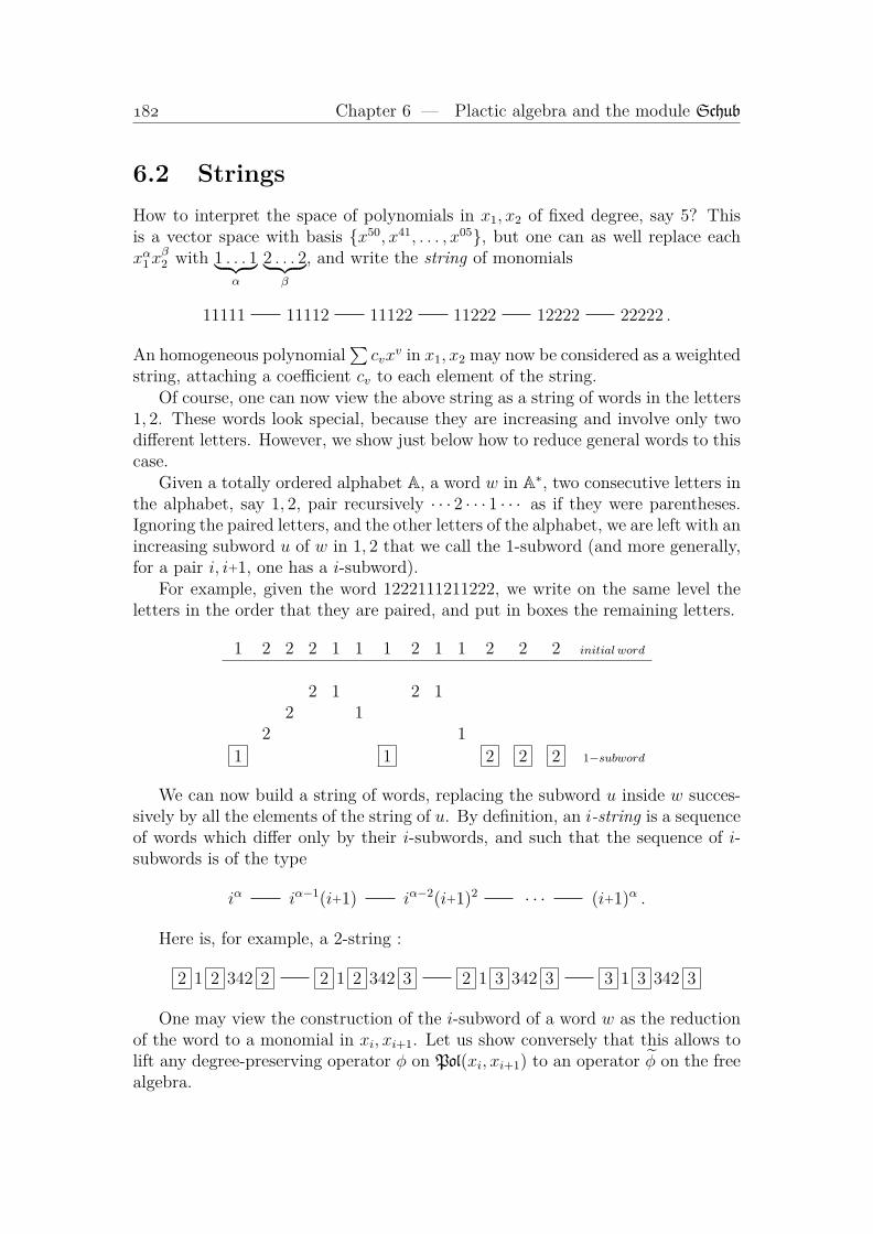
Chapter 6 — Plactic algebra and the module Schub
6.2 StringsHow to interpret the space of polynomials in x1, x2 of fixed degree, say 5? Thisis a vector space with basis x50, x41, . . . , x05, but one can as well replace eachxα1x
β2 with 1 . . . 1︸ ︷︷ ︸
α
2 . . . 2︸ ︷︷ ︸β
, and write the string of monomials
11111 11112 11122 11222 12222 22222 .
An homogeneous polynomial∑cvx
v in x1, x2 may now be considered as a weightedstring, attaching a coefficient cv to each element of the string.
Of course, one can now view the above string as a string of words in the letters1, 2. These words look special, because they are increasing and involve only twodifferent letters. However, we show just below how to reduce general words to thiscase.
Given a totally ordered alphabet A, a word w in A∗, two consecutive letters inthe alphabet, say 1, 2, pair recursively · · · 2 · · · 1 · · · as if they were parentheses.Ignoring the paired letters, and the other letters of the alphabet, we are left with anincreasing subword u of w in 1, 2 that we call the 1-subword (and more generally,for a pair i, i+1, one has a i-subword).
For example, given the word 1222111211222, we write on the same level theletters in the order that they are paired, and put in boxes the remaining letters.
1 2 2 2 1 1 1 2 1 1 2 2 2 initial word
2 1 2 12 1
2 1
1 1 2 2 2 1−subword
We can now build a string of words, replacing the subword u inside w succes-sively by all the elements of the string of u. By definition, an i-string is a sequenceof words which differ only by their i-subwords, and such that the sequence of i-subwords is of the type
iα iα−1(i+1) iα−2(i+1)2 · · · (i+1)α .
Here is, for example, a 2-string :
2 1 2 342 2 2 1 2 342 3 2 1 3 342 3 3 1 3 342 3
One may view the construction of the i-subword of a word w as the reductionof the word to a monomial in xi, xi+1. Let us show conversely that this allows tolift any degree-preserving operator φ on Pol(xi, xi+1) to an operator φ on the freealgebra.
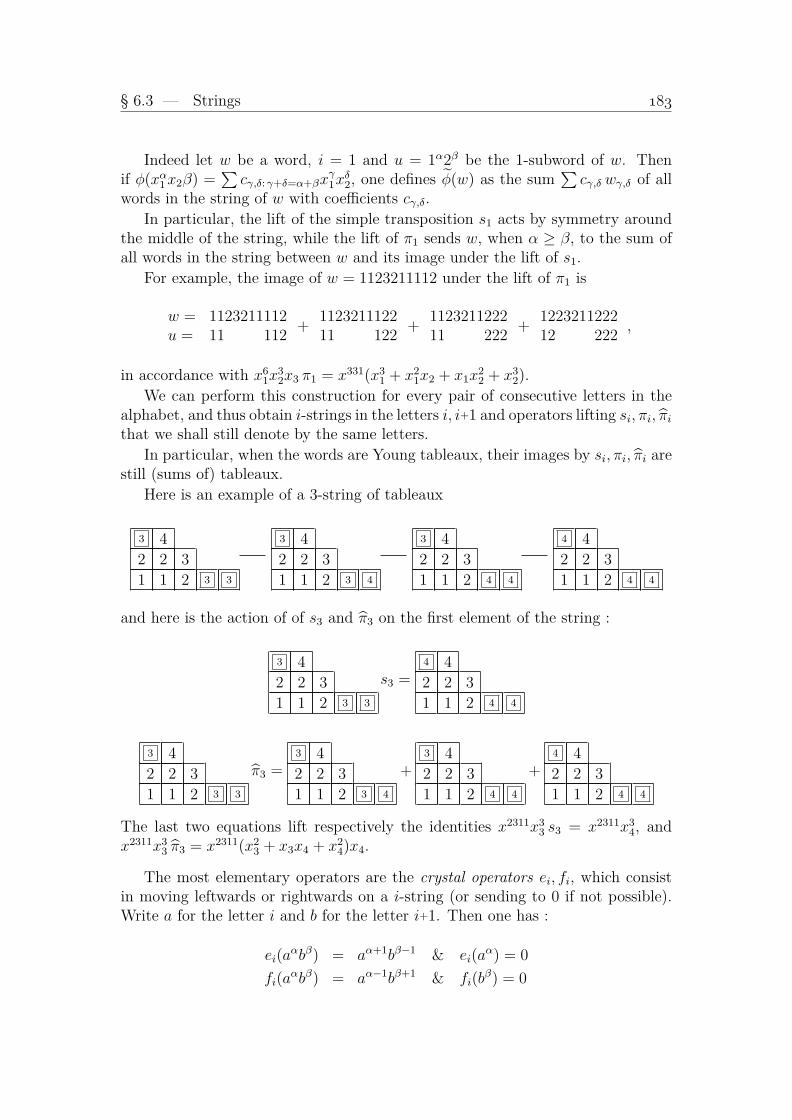
§ 6.3 — Strings
Indeed let w be a word, i = 1 and u = 1α2β be the 1-subword of w. Thenif φ(xα1x2β) =
∑cγ,δ: γ+δ=α+βx
γ1x
δ2, one defines φ(w) as the sum
∑cγ,δ wγ,δ of all
words in the string of w with coefficients cγ,δ.In particular, the lift of the simple transposition s1 acts by symmetry around
the middle of the string, while the lift of π1 sends w, when α ≥ β, to the sum ofall words in the string between w and its image under the lift of s1.
For example, the image of w = 1123211112 under the lift of π1 is
w = 1123211112u = 11 112
+112321112211 122
+112321122211 222
+122321122212 222
,
in accordance with x61x
32x3 π1 = x331(x3
1 + x21x2 + x1x
22 + x3
2).We can perform this construction for every pair of consecutive letters in the
alphabet, and thus obtain i-strings in the letters i, i+1 and operators lifting si, πi, πithat we shall still denote by the same letters.
In particular, when the words are Young tableaux, their images by si, πi, πi arestill (sums of) tableaux.
Here is an example of a 3-string of tableaux
3 4
2 2 3
1 1 2 3 3
3 4
2 2 3
1 1 2 3 4
3 4
2 2 3
1 1 2 4 4
4 4
2 2 3
1 1 2 4 4
and here is the action of of s3 and π3 on the first element of the string :
3 4
2 2 3
1 1 2 3 3
s3 =4 4
2 2 3
1 1 2 4 4
3 4
2 2 3
1 1 2 3 3
π3 =3 4
2 2 3
1 1 2 3 4
+3 4
2 2 3
1 1 2 4 4
+4 4
2 2 3
1 1 2 4 4
The last two equations lift respectively the identities x2311x33 s3 = x2311x3
4, andx2311x3
3 π3 = x2311(x23 + x3x4 + x2
4)x4.
The most elementary operators are the crystal operators ei, fi, which consistin moving leftwards or rightwards on a i-string (or sending to 0 if not possible).Write a for the letter i and b for the letter i+1. Then one has :
ei(aαbβ) = aα+1bβ−1 & ei(a
α) = 0
fi(aαbβ) = aα−1bβ+1 & fi(b
β) = 0

Chapter 6 — Plactic algebra and the module Schub
6.3 Free key polynomialsBeware that the lifted si’s satisfy the braid relations according to [118], but notdo the πi’s. It is proved2 in [126] that one can however lift the key polynomials tothe free algebra, so that the following definition is consistent (we keep the word“polynomial” for these elements of the free algebra, but distinguish them by thenotations KFv , KFv ).
Definition 6.3.1. The free key polynomials KFv , KFv , indexed by v ∈ N∞, aredefined recursively as follows. If v is dominant, then
KFv = KFv = · · · 3v32v21v1 .
Otherwise, if v and i are such that vi > vi+1, then
KFvsi = KFv πi & KFvsi = KFv πi .
We display below the decomposition, in the basis KFu , of the sum of all tableauxof shape [2, 1] on three letters, which is equal to sF21(3) = KF012
3.
KF210 = 21 1
oooooooOOOOOOO
OOOOOOO
KF120 = 21 2
KF201 = 31 1
KF102 = 21 3
+ 31 3
OOOOOOO
KF021 = 31 2
+ 32 2
oooooooooooooo
KF012 = 32 3
Since Kv : v ∈ Nn is a linear basis of Pol(n), we have therefore lifted thering of polynomials into the free algebra, as a free Z-module. Rather than usingthe free algebra, we will mostly use a quotient algebra, the plactic algebra, whichis defined in the next section.
Column tableaux belong to our family. Indeed, let v ∈ 0, 1n. Suppose knownthat KFv = nvn · · · 1v1 , and let i be such that vi = 1, vi+1 = 0 (concanating 0 tothe right of v if needed). Then the image of KFv under πi, which by definition is
2One directly shows that either Proposition 6.6.1 or Proposition 6.6.2 is compatible with theaction of πi or πi.
3The corresponding functions in Pol are Y012 = K012 = K012 + K021 + K102 + K201 + K120 +K210.
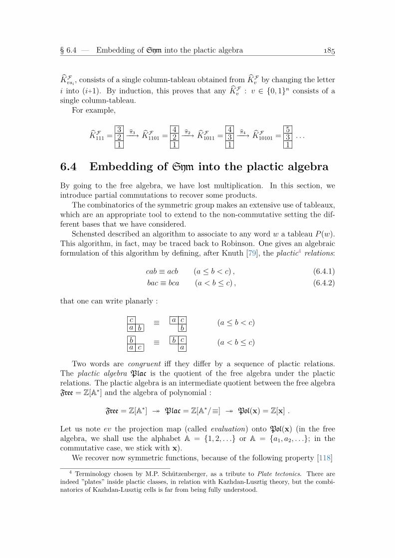
§ 6.4 — Embedding of Sym into the plactic algebra
KFvsi , consists of a single column-tableau obtained from KFv by changing the letteri into (i+1). By induction, this proves that any KFv : v ∈ 0, 1n consists of asingle column-tableau.
For example,
KF111 =321
bπ3−−→ KF1101 =421
bπ2−−→ KF1011 =431
bπ4−−→ KF10101 =531. . .
6.4 Embedding of Sym into the plactic algebraBy going to the free algebra, we have lost multiplication. In this section, weintroduce partial commutations to recover some products.
The combinatorics of the symmetric group makes an extensive use of tableaux,which are an appropriate tool to extend to the non-commutative setting the dif-ferent bases that we have considered.
Schensted described an algorithm to associate to any word w a tableau P (w).This algorithm, in fact, may be traced back to Robinson. One gives an algebraicformulation of this algorithm by defining, after Knuth [79], the plactic4 relations:
cab ≡ acb (a ≤ b < c) , (6.4.1)bac ≡ bca (a < b ≤ c) , (6.4.2)
that one can write planarly :
ca b
≡ a cb
(a ≤ b < c)
ba c
≡ b ca
(a < b ≤ c)
Two words are congruent iff they differ by a sequence of plactic relations.The plactic algebra Plac is the quotient of the free algebra under the placticrelations. The plactic algebra is an intermediate quotient between the free algebraFree = Z[A∗] and the algebra of polynomial :
Free = Z[A∗] Plac = Z[A∗/≡] Pol(x) = Z[x] .
Let us note ev the projection map (called evaluation) onto Pol(x) (in the freealgebra, we shall use the alphabet A = 1, 2, . . . or A = a1, a2, . . .; in thecommutative case, we stick with x).
We recover now symmetric functions, because of the following property [118]4 Terminology chosen by M.P. Schützenberger, as a tribute to Plate tectonics. There are
indeed ”plates” inside plactic classes, in relation with Kazhdan-Lusztig theory, but the combi-natorics of Kazhdan-Lusztig cells is far from being fully understood.

Chapter 6 — Plactic algebra and the module Schub
Proposition 6.4.1. The ring Sym(x) is canonically embedded into the placticalgebra, by sending a Schur function sλ(x) to the sum sFλ of all tableaux of shapeλ.
As a consequence, any algebraic identity in Sym has a non-commutative in-terpretation in the plactic algebra.
For example, the product of two Schur functions
sλ(x)sµ(x) =∑ν
cνλ,µ sν(x)
is described by a certain rule due to Littlewood and Richardson. However, theequation
sFλ (A)sFµ (A) =∑ν
cνλ,µ sFν (A)
gives more information : the coefficient cνλ,µ is the number of factorizations (in theplactic algebra) of any given tableau of t shape ν into a product of two tableauxof respective shapes λ and µ:
t being of shape ν, one has cνλ,µ = #(
(t1, t2) : t1t2 ≡ t, sh(t1) = λ, sh(t2) = µ).
The original rule is the case where one takes t a Yamanouchi tableau5, i.e. t =· · · 3ν3 2ν2 1ν1 = KFν .
For example , to find the multiplicity of s6531 in the product s421s422, one can
start with the Yamanouchi tableau 41332516, which planarly displays as43 3 32 2 2 2 21 1 1 1 1 1
,
into a product of two tableaux of respective shapes [4, 2, 1] and [4, 2, 2]. There arethree such products
32 21 1 2 4
3 32 21 1 1 1
,32 41 1 2 2
3 32 21 1 1 1
,42 31 1 2 2
3 32 21 1 1 1
,
and this is one way of finding, according to the original rule of Littlewood &Richardson, that the multiplicity c6531
421,422 is equal to 3. But one could as well
have factorized43 4 42 3 3 4 41 2 2 3 3 4
into the products
43 42 3 4 4
3 42 31 2 3 4
,43 42 3 4 4
4 42 31 2 3 3
,43 42 3 4 4
4 43 31 2 2 3
.
5A Yamanouchi word is a word w such that for every factorization w = w′w′′, then the rightfactor is such that |w′′|1 ≥ |w′′|2 ≥ |w′′|3 ≥ 0. In particular, for any partition λ, there is onlyone Yamanouchi word which is a tableau of shape λ, and it is equal to . . . 2λ21λ1 .

§ 6.5 — Embedding of Sym into the plactic algebra
Many determinants occur in the theory of symmetric functions. They giveelements of Plac, once one decides to expand them in some arbitrary order (thanksto the plactic relations, the elements do not depend of the choice of the order).
Take for example the Jacodi-Trudi determinant expressing a Schur functionin terms of complete functions. Replace the sum of (unordered) terms sλ =∑±hihj · · ·hk by the sum
∑±sFi sFj · · · sFk . Then, in Plac, one has
sFλ =∑±sFi sFj · · · sFk .
For example, the determinant
s2,2,1 =
∣∣∣∣∣∣h2 h3 h4
h1 h2 h3
0 1 h1
∣∣∣∣∣∣can be expanded as h2h2h1 − h2h3 − h1h3h1 + h1h4 and the element
sF2 sF1 sF2 − sF2 sF3 − sF1 sF3 sF1 + sF1 s
F4
is equal to sF2,2,1. All words which are not congruent to a tableau of shape [2, 2, 1]cancel out.
Tableaux can be interpreted as non-intersecting paths. In that set-up, onerecovers properties of (binomial) determinants that Gessel and Viennot[54] obtainby producing an involution which eliminates intersecting paths, instead of havingrecourse to the plactic relations.
The same function as above is also a determinant of hooks :
s2,2,1 =
∣∣∣∣∣ s2,1,1 s2
s1,1,1 s1
∣∣∣∣∣which can be expanded as s2,1,1s1 − s1,1,1s2. The reader can check that, in fourvariables,
sF2,1,1sF1 − sF1,1,1sF2 =
(321 1
+321 2
+321 3
+421 4
+321 4
+421 1
+421 2
+
431 3
+421 3
+431 4
+431 1
+432 4
+432 3
+432 2
+431 2
)(1 + 2 + 3 + 4
)−
(321
+421
+431
+432
)(1 1 + 2 2 + 1 2 + 1 3 + 3 3 + 2 3
+ 4 4 + 3 4 + 2 4 + 1 4
)is still equal to sF2,2,1, the words which are not congruent to a tableau of shape[2, 2, 1] eliminating two by two.

Chapter 6 — Plactic algebra and the module Schub
6.5 Keys and jeu de taquin on columnsThe jeu de taquin on two-columns tableaux produces a contretableau6 with twocolumns, or conversely. Starting from a tableau with r columns, repeating the jeude taquin on pairs of adjacent columns, one produces r! objects7. Here follows anexample of the plactic class of a tableau with three columns of different lengths :
5 61 3
2 4−→
51 3 6
42
53 61 2 4
1 5 63 4
2
531 2 6
4
−→1 5
3 62 4
Given a tableau t with r columns, and the r! words w = w1 · · ·wr (factorizedas a product of columns) obtained by the jeu de taquin, the set of right columnsC(t) = wr is totally ordered by inclusion. The (right) key of t is defined to bethe tableau of the same shape as t with columns in C(t), or, equivalently, and thisis what we shall keep in most cases, to be the exponent of the evaluation of thiskey-tableau.
key = set of columns embedded into each other⇔ tableau congruent to some word of type . . . 3v32v21v1
⇔ monomial xv = xv11 xv22 . . .
⇔ weight v = [v1, v2, . . . ].
For example, for t =53 61 2 4
, one reads from the preceding hexagon
C(t) =
4 , 6
4,
642
⇔
64 62 4 4
⇔ x2x34x
26 ⇔ [0, 1, 0, 3, 0, 2]
The fact that one has an action of the symmetric group on the columns ofa tableau has for consequence that one can compute the key in several steps,replacing an arbitrary block of left columns by their key.
6skew tableau with outer shape a rectangle.7Reading them by columns, they are the only words in the plactic class of the tableau which
are products of columns of lengths a permutation of the lengths of the columns of the originaltableau.
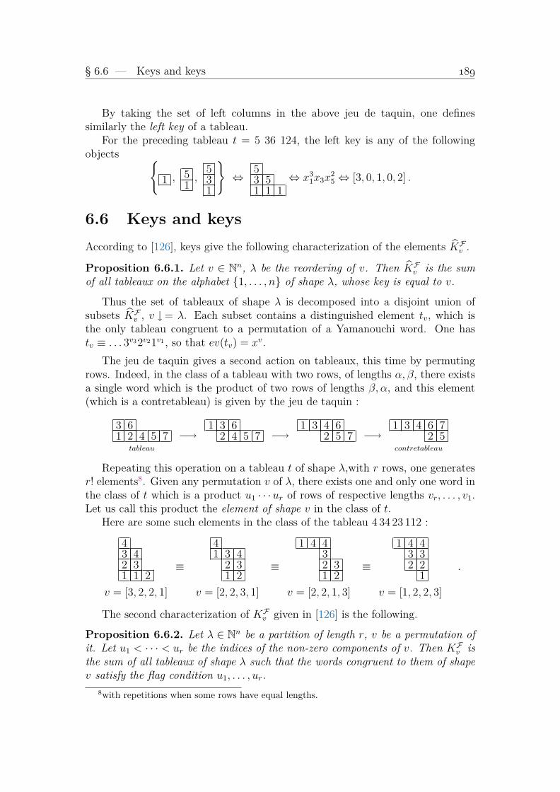
§ 6.6 — Keys and keys
By taking the set of left columns in the above jeu de taquin, one definessimilarly the left key of a tableau.
For the preceding tableau t = 5 36 124, the left key is any of the followingobjects
1 , 51,
531
⇔
53 51 1 1
⇔ x31x3x
25 ⇔ [3, 0, 1, 0, 2] .
6.6 Keys and keysAccording to [126], keys give the following characterization of the elements KFv .
Proposition 6.6.1. Let v ∈ Nn, λ be the reordering of v. Then KFv is the sumof all tableaux on the alphabet 1, . . . , n of shape λ, whose key is equal to v.
Thus the set of tableaux of shape λ is decomposed into a disjoint union ofsubsets KFv , v ↓= λ. Each subset contains a distinguished element tv, which isthe only tableau congruent to a permutation of a Yamanouchi word. One hastv ≡ . . . 3v32v21v1 , so that ev(tv) = xv.
The jeu de taquin gives a second action on tableaux, this time by permutingrows. Indeed, in the class of a tableau with two rows, of lengths α, β, there existsa single word which is the product of two rows of lengths β, α, and this element(which is a contretableau) is given by the jeu de taquin :
3 61 2 4 5 7
tableau
−→1 3 6
2 4 5 7 −→1 3 4 6
2 5 7 −→1 3 4 6 7
2 5contretableau
Repeating this operation on a tableau t of shape λ,with r rows, one generatesr! elements8. Given any permutation v of λ, there exists one and only one word inthe class of t which is a product u1 · · ·ur of rows of respective lengths vr, . . . , v1.Let us call this product the element of shape v in the class of t.
Here are some such elements in the class of the tableau 4 34 23 112 :
43 42 31 1 2
v = [3, 2, 2, 1]
≡
41 3 4
2 31 2
v = [2, 2, 3, 1]
≡
1 4 432 31 2
v = [2, 2, 1, 3]
≡
1 4 43 32 2
1
v = [1, 2, 2, 3]
.
The second characterization of KFv given in [126] is the following.
Proposition 6.6.2. Let λ ∈ Nn be a partition of length r, v be a permutation ofit. Let u1 < · · · < ur be the indices of the non-zero components of v. Then KFv isthe sum of all tableaux of shape λ such that the words congruent to them of shapev satisfy the flag condition u1, . . . , ur.
8with repetitions when some rows have equal lengths.
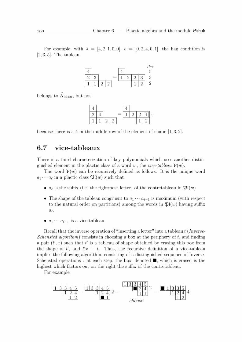
Chapter 6 — Plactic algebra and the module Schub
For example, with λ = [4, 2, 1, 0, 0], v = [0, 2, 4, 0, 1], the flag condition is[2, 3, 5]. The tableau
4
2 3
1 1 2 2
≡4
1 2 2 3
1 2
flag
532
belongs to K02401, but not
4
2 4
1 1 2 2
≡4
1 2 2 4
1 2
,
because there is a 4 in the middle row of the element of shape [1, 3, 2].
6.7 vice-tableauxThere is a third characterization of key polynomials which uses another distin-guished element in the plactic class of a word w, the vice-tableau V(w).
The word V(w) can be recursively defined as follows. It is the unique worda1 · · · a` in a plactic class Pl(w) such that
• a` is the suffix (i.e. the rightmost letter) of the contretableau in Pl(w)
• The shape of the tableau congruent to a1 · · · a`−1 is maximum (with respectto the natural order on partitions) among the words in Pl(w) having suffixa`.
• a1 · · · a`−1 is a vice-tableau.
Recall that the inverse operation of “inserting a letter” into a tableau t (Inverse-Schensted algorithm) consists in choosing a box at the periphery of t, and findinga pair (t′, x) such that t′ is a tableau of shape obtained by erasing this box fromthe shape of t′, and t′x ≡ t. Thus, the recursive definition of a vice-tableauimplies the following algorithm, consisting of a distinguished sequence of Inverse-Schensted operations : at each step, the box, denoted , which is erased is thehighest which factors out on the right the suffix of the contretableau.
For example
1 3 3 4 51 2 4
1 2≡
1 3 3 4 51 2 4 1
2 ≡1 3 3 4 5 2 4
1 12
choose!
≡ 1 3 3 5
1 2 41 2
4

§ 6.8 — Ehresmann tableaux
shows thatV(13345 124 12) = V(13345 24 11) · 2 .
Iterating, one finds a word that one factors into its maximal rows, and that oncan display as a skew tableau
V(13345 124 12) =3 51 2 3 4 4
1 1 2, shape [0, 3, 0, 5, 2] .
The shape of the vice-tableau is the sequence v1, v2, . . . , vn, where vi is the lengthof the (single) row ending with a letter i. Empty rows have to be recorded !
The original unpublished characterization of key polynomials is the following.Proposition 6.7.1. Given v ∈ Nn, then KFv is the sum, in Plac, of all vice-tableaux of shape v.
For example, KF01302 =5 51 3 3
2+
4 51 3 3
2+
5 53 3 3
2+
4 53 3 3
2+
5 52 3 3
2+
4 52 3 3
2. This sum is congruent to the following sum of tableaux, which is more difficult to
identify at first glance :53 51 2 3
+43 51 2 3
+53 52 3 3
+43 52 3 3
+53 52 2 3
+43 52 2 3
.
One has a similar notion of left vice-tableau, by iterating the operation: factort into xt′ in the plactic monoid, in such a way that x is the first letter of thetableau, and the shapes of t and t′ differ by a box which is the lowest possible.
The same word as above gives
3 52 3 41 1 1 2 4
≡ 35 2 3 41 1 1 2 4
≡3
3 52 4 1 1 1 2 4
choose!
≡ 13 52 3 41 1 2 4
and, iterating, the left vice-tableau
3 3 52 41 1 1 2 4
.
6.8 Ehresmann tableauxGiven a permutation σ ∈ Sn, the sequence σ1, σ1, σ2, . . . , σ1, . . . , σn is anincreasing flag of subsets of 1, . . . , n, and may be interpreted as the sequence ofcolumns of a contretableau, ordering each set decreasingly, or of a tableau, readingthe flag from right to left.
σ = [3, 5, 1, 4, 2]⇒3 5 5 5 5
3 3 4 41 3 3
1 21
≡54 53 4 52 3 3 51 1 1 3 3
.

Chapter 6 — Plactic algebra and the module Schub
These tableaux, that we shall denote E(σ), were used by Ehresmann [35] todescribe a cellular decomposition of the flag variety relative to the linear groupGLn(C). Ehresmann described the attachment of cells by introducing an order:σ ≤ ζ if and only if E(σ) ≤ E(ζ) componentwise. This order on permutationsis the same as the one obtained by taking subwords of reduced decompositions,and usually called the Bruhat order, or strong order9. A tableau t on the letters1, . . . , n of shape [n, . . . , 1] has a key which is some E(σ), and we shall denote thispermutation ’oooooo (t). More generally, if t is of arbitrary shape, the set of columns ofits key may be completed in the set of columns of an Ehresmann tableau, and wedefine ’oooooo (t) to be the permutation σ such that E(σ) is (componentwise) minimumamong those E(ζ) containing the columns of the key.
For example,42 3 41 1 2
≡2 4 41 1 3
2has key
43 4 42 2 2
, and
’oooooo
43 42 3 41 2 2 2
= [2, 4, 3, 1] is the minimum Ehresmann tableau containing
the columns [4, 2], [4, 3, 2].Similarly, one can take the maximum Ehresmann tableau containing the columns
of the left key of a tableau, and one obtains a second permutation ’oooooo left(t).Given two tableaux t, u of shapes λ, µ, the product t u is defined to be frank if
the shape of the tableau congruent to tu is equal to the sum λ+ µ. The action ofthe symmetric group on the columns of a tableau seen above has exhibited frankproducts of columns.
In the case where t and u are single columns, tu is frank iff tu is a column-tableau (case `(t) ≥ `(u)) or a column contretableau (case `(t) ≤ `(u)). Moregenerally, it is shown in [126, Th.2.8] that tu is frank iff for every permutationst ≡ t1 . . . tk, u ≡ u1 . . . ur of the columns of t and u respectively, then the productof two columns tku1 is frank. Thus, the test to be frank reduces to the case ofpairs of columns.
The notion of frank product is closely related to the Ehresmann-Bruhat order,as shows the following lemma given in [126, Th.2.10].
Lemma 6.8.1. Given two tableaux t, u of respective shapes λ, µ, then the producttu is frank if and only if ’oooooo (t) ≤ ’oooooo left(u).
The order on Ehresmann tableaux is the componentwise order. One couldthink of avoiding the construction of keys, and directly use the componentwiseorder on tableaux of a given shape. This structure on tableaux is not related to
9Ehresmann did not mention permutations, but was using flags of Plücker coordinates,in other words, was using Ehresmann tableaux. The terminology “Bruhat order” is due toVerma[190], because of the Bruhat decomposition BσB, of GLn(C), B being the Borel sub-group of triangular matrices. I interviewed Bruhat, who, of course, did not claim any paternityabout the Bruhat order.
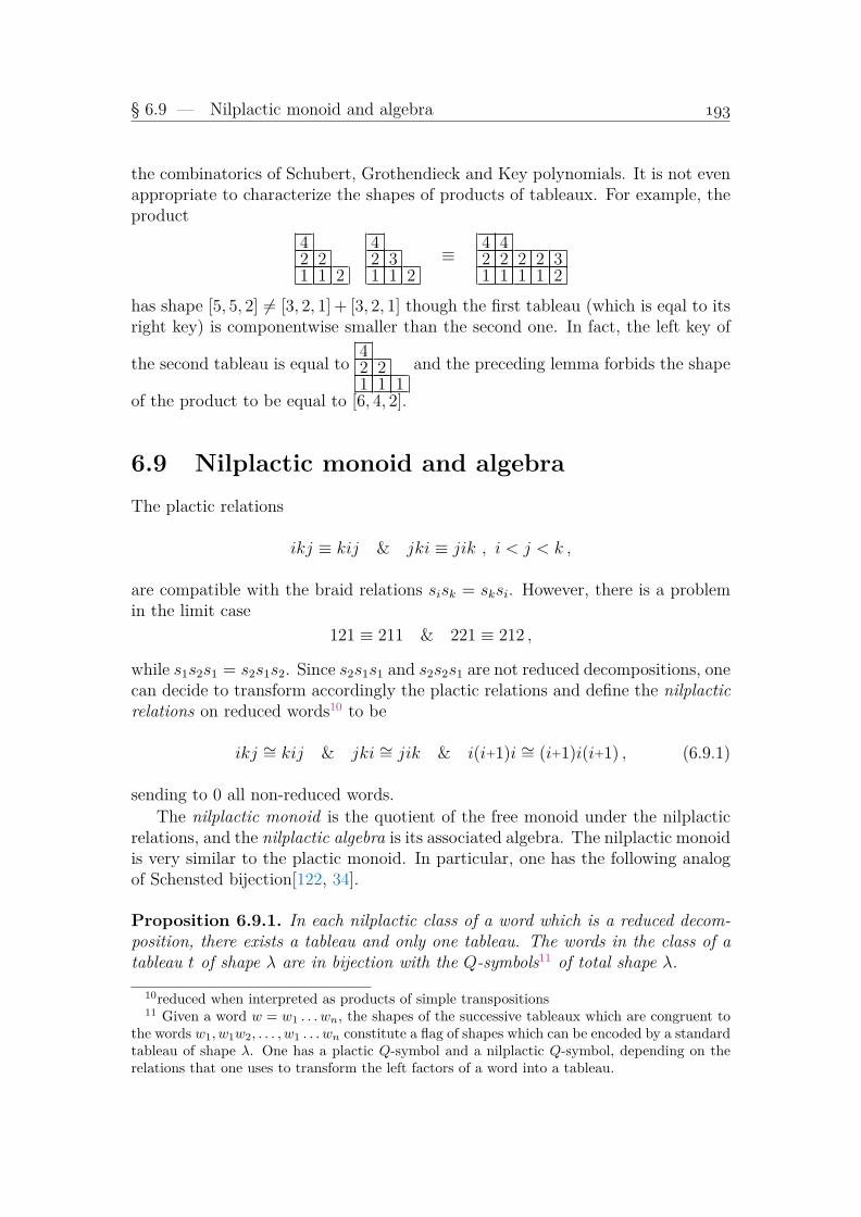
§ 6.9 — Nilplactic monoid and algebra
the combinatorics of Schubert, Grothendieck and Key polynomials. It is not evenappropriate to characterize the shapes of products of tableaux. For example, theproduct
42 21 1 2
42 31 1 2
≡4 42 2 2 2 31 1 1 1 2
has shape [5, 5, 2] 6= [3, 2, 1] + [3, 2, 1] though the first tableau (which is eqal to itsright key) is componentwise smaller than the second one. In fact, the left key of
the second tableau is equal to42 21 1 1
and the preceding lemma forbids the shape
of the product to be equal to [6, 4, 2].
6.9 Nilplactic monoid and algebraThe plactic relations
ikj ≡ kij & jki ≡ jik , i < j < k ,
are compatible with the braid relations sisk = sksi. However, there is a problemin the limit case
121 ≡ 211 & 221 ≡ 212 ,
while s1s2s1 = s2s1s2. Since s2s1s1 and s2s2s1 are not reduced decompositions, onecan decide to transform accordingly the plactic relations and define the nilplacticrelations on reduced words10 to be
ikj ∼= kij & jki ∼= jik & i(i+1)i ∼= (i+1)i(i+1) , (6.9.1)
sending to 0 all non-reduced words.The nilplactic monoid is the quotient of the free monoid under the nilplactic
relations, and the nilplactic algebra is its associated algebra. The nilplactic monoidis very similar to the plactic monoid. In particular, one has the following analogof Schensted bijection[122, 34].
Proposition 6.9.1. In each nilplactic class of a word which is a reduced decom-position, there exists a tableau and only one tableau. The words in the class of atableau t of shape λ are in bijection with the Q-symbols11 of total shape λ.
10reduced when interpreted as products of simple transpositions11 Given a word w = w1 . . . wn, the shapes of the successive tableaux which are congruent to
the words w1, w1w2, . . . , w1 . . . wn constitute a flag of shapes which can be encoded by a standardtableau of shape λ. One has a plactic Q-symbol and a nilplactic Q-symbol, depending on therelations that one uses to transform the left factors of a word into a tableau.

Chapter 6 — Plactic algebra and the module Schub
The correspondence between the plactic and nilplactic classes can be realizedby describing a bijection exchanging the two congruences. I gave such a corre-spondence with M.P. Schützenberger under the name plaxification, but Reiner andShimozono obtained a much more elegant description. The plactification Pl is atransformation on words which is defined recursively as follows, starting with theempty word which is exchanged with itself.(
w = iw′ , Pl(w′) = η)⇒ Pl(w) = i (η)si ,
where si acts as defined in the preceding section.The plactification can be visualized as moving a cursor (here a box) from right
to left, a pointed letter acting as a simple transposition si on the factor on itsright. For example, Pl([3, 2, 1, 3, 2, 4, 3, 4] is the last word in the following chain
[3, 2, 1, 3, 2, 4, 3, 4 ] = [3, 2, 1, 3, 2, 4, 3, 4]
[3, 2, 1, 3, 2, 4, 3 , 4] = [3, 2, 1, 3, 2, 4, 3, 3]
[3, 2, 1, 3, 2, 4 , 3, 3] = [3, 2, 1, 3, 2, 4, 3, 3]
[3, 2, 1, 3, 2 , 4, 3, 3] = [3, 2, 1, 3, 2, 4, 2, 2]
[3, 2, 1, 3 , 2, 4, 2, 2] = [3, 2, 1, 3, 2, 3, 2, 2]
[3, 2, 1 , 3, 2, 3, 2, 2] = [3, 2, 1, 3, 1, 3, 1, 1]
[3, 2 , 1, 3, 1, 3, 1, 1] = [3, 2, 1, 2, 1, 2, 1, 1]
[ 3 , 2, 1, 2, 1, 2, 1, 1] = [3, 2, 1, 2, 1, 2, 1, 1]
Needless to add that the morphism inverse to Pl is obtained by moving a cursorfrom left to right, and acting accordingly on the right factor.
Proposition 6.9.2. [175] The morphism Pl() sends the nilplactic class of a re-duced word to a plactic class, preserving the Q-symbol.
For example, the nilplactic class of [2, 3, 1, 2, 3] is sent to the plactic class of[2, 2, 1, 1, 1].
23123
21323
vvvvvH
HH
12312
HH
H21232
vvvvv
12132
Pl−→22111
21211
vvvvvH
HH
12211
HH
H21121
vvvvv
12121
One has still an action of the symmetric group on the columns of a nilplactictableau, so that one can define a right nilplactic key or a left nilplactic key.

§ 6.9 — Nilplactic monoid and algebra
For example, the hexagon
2 41 3
2 3−→
21 2 4
32
42 31 2 3
1 2 41 3
2
421 2 3
2
−→1 4
2 31 2
gives the left key42 21 1 1
and the right key43 32 2 3
.
Notice that, because the tranpose of a nilplactic tableau is still a nilplactictableau, one has also two other keys, the bottom key, and the top key, obtainedby transposing rows using the niplactic relations.
Since two reduced words which are nilplactically congruent are reduced de-compositions of the same permutation, the set of reduced decompositions of apermutation decomposes into a union of nilplactic classes, that one can charac-terize by the tableau that each of them contain. As a consequence, the number ofreduced decompositions of a given permutation is a sum of cardinals of plactic ornilplactic classes12 The problem of determining the number of reduced decomposi-tions of a permutation has been considered by Stanley [184] who have reformulatedit in terms of certain symmetric functions which are now called Stanley symmetricfunctions, and are the stable parts of Schubert polynomials. Edelman and Greene[34] gave a more combinatorial solution in terms of balanced tableaux, using alsothe nilplactic relations. I preferred to use here the point of view of the note [122],supplemented by the plaxification.
For example, there are 414 = 168+84+162 reduced decompositions of the per-mutation [3, 1, 7, 6, 2, 4, 5], which regroup into three nilplactic classes. We writebelow these three tableaux, as well as their images under Pl.
65 62 4 51 3 4
Pl−→65 52 4 41 2 2
,5 64 52 41 3 4
Pl−→5 64 52 41 2 2
,
654 62 51 3 4
Pl−→654 52 41 2 2
cardinalityof each class
168 84 162
12a plactic or nilplactic class containing a tableau of shape λ has cardinality the number ofstandard tableaux of shape λ. This number is also the dimension of the irreducible representationof index λ of the symmetric group.

Chapter 6 — Plactic algebra and the module Schub
6.10 Lifting Pol to a submodule of Plac
Let us first consider the space of polynomials Pol in x1, x2, . . . , xn, . . . (no limit onn), as an inductive limit of Pol(xn), with xn = x1, . . . , xn.
We have defined flag-elementary functions Pv(x). There is only one naturalway to lift an elementary symmetric function to the free algebra. It must be,in agreement with the definition of free key polynomials, the sum of all strictlydecreasing words of a given degree in a totally ordered alphabet, that is to saythe sum of all tableaux whose shape is a column of a given length :
ek(xr) ←→ Λk(r) = sum of all decreasing words of length k in 1, . . . , r .By product, for any v ∈ Nn, v ≤ [n−1, . . . , 0], define in the free algebra
PFv := Λv1(n−1)Λv2(n−2) · · ·Λvn−1(1)Λvn(0) .
The Z-span of all PFv in the quotient algebra Plac is denoted Schub, and istherefore a lift of Pol. Indeed, every polynomial is lifted to Plac by expanding itinto the basis Pv, then formally changing every Pv into PFv .
The word 21 = Λ2(2) belongs to Schub, but not the word 12, because ithas the same evaluation. Neither does the word 22 belong to Schub, becausex2
2 = P1100 − P2000 − P200 lifts into
(1+2+3)(1+2)− (21+31+32)− (1+2)1 = 22 + 12− 21 = 2 2 + 1 2 − 21.
We have a problem now. We have already lifted Pol to the free algebra bydefining free key polynomials, we must ensure that the two elements correspondingin Plac to a polynom f =
∑cvPv =
∑duKu coincide.
Let us prove that Schub is the image in Plac of the product ring
· · · ⊗Sym(3)⊗Sym(2)⊗Sym(1) .
First, the lift of a Schur function sλ(xn), in terms of PFv , is given by the orderedexpansion of a determinant Λu(m/m− 1/ · · · /n), where u is the reordering ofλ∼. Since Λi(m) = Λi(m−1) + mΛi−1(m−1), the determinant is the sum ofΛu(m−1/m−1/ · · · /n) and a determinant with first two rows∣∣∣∣· · · mΛi(m−1) · · ·
· · · Λi(m−1) · · ·
∣∣∣∣ .However, all the Λi(m−1) commute between themselves in Plac, and thereforethis second determinant is null. Repeating this transformation, one sees that theoriginal determinant is equal to Λu(n/ · · · /n), and is therefore equal to the sumsFλ (n) of all tableaux of shape λ in the alphabet n = 1, . . . , n.
The intermediate expression Λu(n+1/ · · · /n+1/n) shows that sFλ (n) is alsoequal to a sum
∑ν,i±sFν (n+1)Λi(n). A product sFµ (n+1)sFλ (n) may therefore be
expressed as a sum of products sFµ (n+1)sFν (n+1)Λi(n), then of products sFη (n+1)Λi(n).
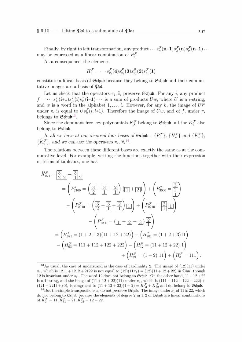
§ 6.10 — Lifting Pol to a submodule of Plac
Finally, by right to left transformation, any product · · · sFη (n+1)sFλ (n)sFν (n−1) · · ·may be expressed as a linear combination of PFv .
As a consequence, the elements
HFv = · · · sFv4(4)sFv3(3)sFv2(2)sFv1(1)
constitute a linear basis of Schub because they belong to Schub and their commu-tative images are a basis of Pol.
Let us check that the operators πi, πi preserve Schub. For any i, any productf = · · · sFλ (i+1)sFµ (i)sFν (i−1) · · · is a sum of products Uw, where U is a i-string,and w is a word in the alphabet 1, . . . , i. However, for any k, the image of Uikunder πi is equal to UsFk (i, i+1). Therefore the image of Uw, and of f , under πibelongs to Schub13.
Since the dominant free key polynomials KFλ belong to Schub, all the KFv alsobelong to Schub.
In all we have at our disposal four bases of Schub : PFv , HFv and KFv ,KFv , and we can use the operators πi, πi14.
The relations between these different bases are exactly the same as at the com-mutative level. For example, writing the functions together with their expressionin terms of tableaux, one has
KF021 = 32 2
+ 31 2
=
(PF2100 =
(32
+ 31
+ 21
)(1 + 2
))+
(PF3000 =
321
)
−
(PF2010 =
(32
+ 31
+ 21
)1
)+
(PF0210 = 2
1 1
)
−
(PF1200 =
(1 + 2 + 3
)21
)=(HF021 = (1 + 2 + 3)(11 + 12 + 22)
)−(HF201 = (1 + 2 + 3)11
)−(HF03 = 111 + 112 + 122 + 222
)−(HF12 = (11 + 12 + 22) 1
)+(HF21 = (1 + 2) 11
)+(HF3 = 111
).
13As usual, the case ot understand is the case of cardinality 2. The image of (12)(11) underπ1, which is 1211 + 1212 + 2122 is not equal to (12)(11π1) = (12)(11 + 12 + 22) in Plac, though12 is invariant under s1. The word 12 does not belong to Schub. On the other hand, 11+12+22is a 1-string, and the image of (11 + 12 + 22)(11) under π1, which is (111 + 112 + 122 + 222) +(121 + 221) + (0), is congruent to (11 + 12 + 22)(1 + 2) = KF03 +KF12 and do belong to Schub.
14But the simple transpositions si do not preserve Schub. The image under s1 of 11 is 22, whichdo not belong to Schub because the elements of degree 2 in 1, 2 of Schub are linear combinationsof KF2 = 11, KF11 = 21, KF02 = 12 + 22.
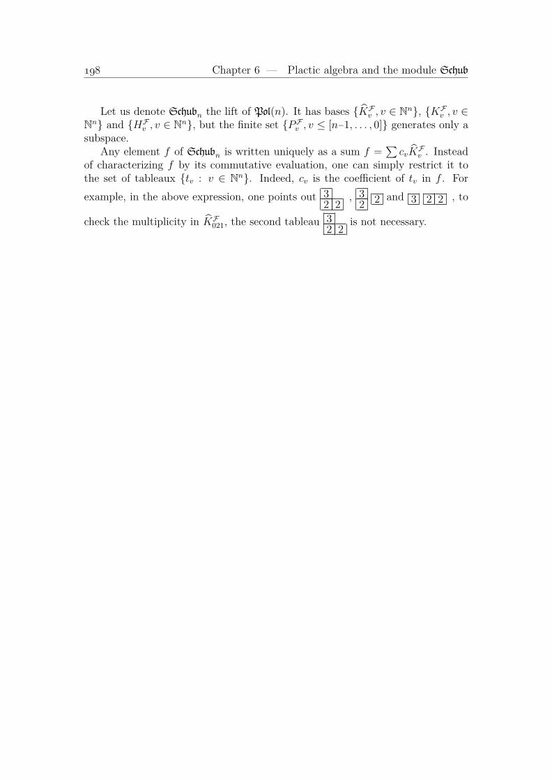
Chapter 6 — Plactic algebra and the module Schub
Let us denote Schubn the lift of Pol(n). It has bases KFv , v ∈ Nn, KFv , v ∈Nn and HFv , v ∈ Nn, but the finite set PFv , v ≤ [n−1, . . . , 0] generates only asubspace.
Any element f of Schubn is written uniquely as a sum f =∑cvK
Fv . Instead
of characterizing f by its commutative evaluation, one can simply restrict it tothe set of tableaux tv : v ∈ Nn. Indeed, cv is the coefficient of tv in f . Forexample, in the above expression, one points out 3
2 2, 3
2 2 and 3 2 2 , to
check the multiplicity in KF021, the second tableau 32 2
is not necessary.

§ 6.11 — Allowable products in Schub
6.11 Allowable products in Schub
We have just stated that any product of the type · · · sFλ (k+1)sFµ (k)sFν (k−1) · · ·belongs to Schub. The weakly decreasing condition on alphabets is necessary. Forexample, the product
sF1 (3)sF1 (2) = KF02 +KF011
belongs to Schub, but
sF1 (2)sF1 (3) = KF02 +KF11 + 1 3 + 2 3
does not belong to it.Let us show that right multliplication by a column k . . . 1 is permitted.Given k, and any f = · · · sFλ (k+1)sFµ (k)sFν (k−1) · · · sFη (1), its product on the
right by k · · · 1 is equal to
· · · sFλ (k+1)sFµ (k) (k · · · 1) sFν (k−1) · · · sFη (1) ,
because all letters not greater than k commute with the column k · · · 1.By iteration this proves that the product on the right by any KFλ , λ partition,
preserves Schub. Thus, the product in Pol by a dominant monomial xλ, that wehave used many times, lifts to the right multliplication by KFλ .
We have seen that column-tableaux belong to Schub, being equal to some KFvwith v ∈ 1, 0∗. Given n, r, the column (n+r) · · · (n+1) may be expressed15 as alinear combination of PFu,0n . Consequently, for any v ∈ Nn, the product
(n+r) · · · (n+1) KFv
belongs to Schub.For example
43KF02 =
(Λ2(4)− Λ2(3)− Λ1(4)Λ1(2) + Λ1(3)Λ1(2)
)(sF2 (2)− sF2 (1)
)= 4
3
(1 2 + 2 2
)=
431 2
+432 2
belongs to Schub (it is in fact equal to KF0211).One can use the fact that products sFλ (n)KFv , v ∈ Nn, belong to Schubn, to
generalize the Littlewood-Richardson rule.15 Explicitely,
(n+r) · · · (n+1) =∑
u≤[r,1...r−1]
(−1)r−1+`(u)(PFu1,0,u2−1,...,ur−r+1,0n − PFu1,u2−1,...,ur−r+1,0n)
sum over all permutations u below (for the Ehresmann-Bruhat order) [r, 1, . . . , r−1].

Chapter 6 — Plactic algebra and the module Schub
In the case where v = µ is dominant, one has
sFλ (n) tµ =∑
tKFcl(t tµ) ,
sum over all tableaux t of shape λ such that t tµ is congruent to some tableautu. Using the operators πσ, one obtains the product of a Schur function by a keypolynomial in terms of tableaux which are in the orbit of Yamanouchi tableauxunder the symmetric group.
Lemma 6.11.1. Let λ be a partition in Nn, v ∈ Nn, then one has
sFλ (n)KFv =∑
tKFcl(t t′) , (6.11.1)
sum over all tableaux t of shape λ, t′ ∈ KFv , such that t t′ is congruent to sometableau tu.
For example, restricting the products KF012Kv, with v↓= [2, 1, 0], to the termswhich give a key which is a permutation of [1, 2, 3], one has
KF012KF210 →
31 2
21 1
∈ KF321 ,32 2
21 1
∈ KF231 ,31 3
21 1
∈ KF312
,
KF012KF201 →
31 2
31 1
∈ KF312 ,32 3
31 1
∈ KF213
,
KF012KF120 →
21 3
21 2
∈ KF231 ,32 3
21 2
∈ KF132
,
KF012KF021 →
32 3
31 2
∈ KF132 ,32 3
31 2
∈ KF123
,
KF012KF102 →
32 3
21 3
∈ KF123 ,31 3
21 3
∈ KF213
,
while KF012KF012 = KF024 → 0. The sum of all these terms is
KF012KF012 →
∑u:u↑=123
2KFu = 2KF123
in accordance with s221 = 2s321 + . . . . The multiplicity 2 can already be read from
the first product KF012KF210, because KF012K
F210π321 = KF012K
F012. It is therefore the

§ 6.11 — Allowable products in Schub
number of tableaux t of shape [2, 1] such that t t21 be congruent to t321. We areback to the Littlewood-Richardson rule ! Notice that in the product KF012K
F210 one
has now ignored the contributions 322 211 and 313 211 because KF231π321 = 0 =
KF312π321.Linear relations in Schub can be checked by examining their commutative im-
age in Pol, and conversely, any identity in Pol has a non-commutative counterpartin Schub. We already used this property for symmetric polynomials.
For example, we have seen that K02301 has a determinantal expression
S00123(x5,x5,x5,x3,x3) = S123(x5,x3,x3) ,
because [0, 2, 3, 0, 1] is a vexillary code. Expanding
S123(x5,x3,x3) =
∣∣∣∣∣∣K00001 K003 K005
1 K002 K004
0 K001 K003
∣∣∣∣∣∣in any manner, transforming each Kv into KFv after reordering each product intoa decreasing flag, one obtains
KF02301 ≡ KF00001KF002K
F003 −KF00001K
F004K
F001 −KF003K
F003 +KF005K
F001 .
Because K00k = K0k−x3K0,0,k−1, K00k = Kk− (x2+x3)K0,0,k−1 +x2x3K0,0,k−2,
one can transform the preceding determinant into
∣∣∣∣∣∣x1 + x4 + x5 K3 K5
1 K02 K04
0 K001 K003
∣∣∣∣∣∣.Writing x1+x4+x5 = K00001 − K001 + K1, expanding the determinant, and
reordering the products, one obtains a second expression
KF02301 ≡ KF00001KF003K
F02 −KF00001K
F001K
F04 −KF001K
F003K
F02 + (KF001)
2KF04
+KF003KF02K
F1 −KF001K
F04K
F1 −KF003K
F3 +KF001K
F5 .
Apart from the vexillary case, we have met other determinantal expressions.The case treated in Th. ?? has for counterpart in Schub the following lemma(which is a special case of the description of key polynomials).
Lemma 6.11.2. Let v ∈ Nn be dominant, u ∈ Nn be anti-dominant, v//u =[0u1 , v1, 0
u2−u1 , v2, . . . , 0un−un−1 , vn]. Then KFv//u is equal to the sum of all tableaux
of shape v satisfying the flag condition [u1 + 1, . . . , un + n].
For example, for v = [2, 1], u = [1, 3], then v//u is [01, 2, 02, 1], the flag isu + [1, 2] = [2, 5] and KF02001 is equal to the sum of all tableaux c
a bsuch that
b ≤ 2, c ≤ 5.

Chapter 6 — Plactic algebra and the module Schub
6.12 Generating function of Schubert polynomi-als in Schub
According to Cauchy formula (2.10.2), the product Ω =∏
i,j: i+j<n(yj+xi) expandsa sum
∑σ∈Sn
Xσω(y,0)Xσ(x,0). Thus, one can define the Schubert polynomialsin x as the coefficients in the expansion of Ω in the basis of Schubert polynomialsin y. This looks like a circular definition without interest, except that one caneasily lift Ω to an element of Schub, and obtain now the free Schubert polynomialsfrom the commutative ones.
Given n and an alphabet A = a1, . . . , an, one defines
XFω (A,x) =(
(an−1−x1) . . . (a1−x1))(
(an−2−x2) . . . (a1−x2)). . .(
(a1−xn−1)).
Given σ ∈ Sn, the free Schubert polynomial XFσ (A,y) is defined to be thecoefficient of (−1)`(ωσ)Xωσ(x,y) in the expansion of XFω (A,x) in terms of Schubertpolynomials in x,y 16
Since the kernel XFω (A,x) belongs to Schub, the element XFσ (A,y) coincideswith the element defined by expressingXσ(x,y) in any of the basesKv(x), Pv(x), Hv(x),and replacing these polynomials by their lift in Schub.
For example, taking the alphabet A = 1 , 2 , . . . , , persevering in readingcolumnwise, then the coefficient of X213(x,y) in the expansion of
XF321(A,x) =2 −x1
1 −x1 1 −x2,
is equal to
·1 1
+ 2· 1− 2
1 ·− (y1+y2) ·· 1
+ y1y2·· · ≡
(1 − y1
)(1 − y2
).
In the case where σ is dominant, of code λ, the filling of each box of thediagram of λ with the factor i − yj, where (i, j) are the coordinates of the box,still belongs to Schub, and therefore is equal to XFσ (A,y). For example,
XF3412(A,y) =2 −y1 2 −y2
1 −y1 1 −y2
≡ 2 21 1
− (y1+y2)
(21 1
+ 21 2
)+ y1y2
(1 1 + 1 2 + 2 2
)+ (y2
1+y1y2+y22) 2
1− (y2
1y2+y1y22)(
1 + 2)
+ y21y
22 .
16A function of A, x may be expanded in terms of functions of A,x,y, one can use simultane-ously several Schubert bases Xσ(x, z) of Pol(x) with different z.

§ 6.12 — Generating function of Schubert polynomials in Schub
Free Schubert polynomials XFσ (A,y) may be recursively obtained by using thedivided differences in y17. For example
−XF3412(A,y)∂y2 = XF2413(A,y) =
(21 1
+ 21 2
)− y1
(1 1 + 1 2 + 2 2
)− (y1+y2+y3) 2
1+ (y2
1+y1y2 + y1y3)(
1 + 2)− y2
1(y2+y3)
≡(
2 − y1
)(1 − y1
)(2 + 1 − y2 − y3
).
17but defining divided differences in A which would satisfy the braid relations is not feasible.One can however lift formally the action of divided differences on the basis Pv, as is used in[127, 48].

Chapter 6 — Plactic algebra and the module Schub

Chapter 7Schubert and Grothendieck by keys
7.1 Double keys
In the commutative case, we did not define key polynomials in two sets of variables,contrary to Schubert or Grothendieck polynomials, because there was no “good”candidate. In the free world, it is very easy. Indeed, the operators si or πi onwords can be obtained from the operator fi, which changes, whenever possible, aspecific occurence of a letter i in a word w, or a tableau, into i+1. We can act onbiletters (i.e. letters with a superscript). Ignoring the superscripts, we point outsome biletter
(ji
)as in the case of single letters, and we transform it into
(j+1i+1
).
This action does not lift a commutative action.Noticing that the above transformation preserves the difference between su-
perscript and subscript, we can describe directly the transformations on biwordsfrom the case of words: if a letter i is transformed into a letter k, then in the caseof biletters,
(ji
)is transformed into
(j+k−ik
).
Starting with an appropriate word in biletters replacing the word · · · 2λ21λ1 ,and extending the action of πi or πi to biwords, we obtain sums of biwords.
For a partition λ, define
Kλ = Kλ =
(1n
). . .
(λnn
)(1
n−1
). . . . . .
(λn−1
n−1
)... ...(11
). . . . . . . . .
(λ1
1
)By definition, the elements Kv and Kv, when v runs over the set of permuta-
tions of λ, are all the images of Kλ and Kλ under (reduced) products of πi’s (resp.πi’s).
205

Chapter 7 — Schubert and Grothendieck by keys
It seems that not much has been gained by passing to biletters. Writing
KF102 = 2
1 1+ 2
1 2+ 3
1 1+ 2
1 3+ 3
1 3instead of
K102 =
(12
)(
11
) (21
) +
(12
)(
11
) (32
) +
(23
)(
11
) (21
) +
(12
)(
11
) (43
) +
(23
)(
11
) (43
)is, indeed, immediate. But these new functions possess more properties than inthe case of single letters. For example, under the projection(
j
i
)7→ (xi − yj) ,
one obtains polynomials in two sets of variables that we shall still denote Kv.For example, KF021 = 3
2 2+ 3
1 2+ 2
1 2+ 3
1 1+ 2
1 1is transformed into
five tableaux of biletters which compose K021 and become
x3−y2
x2−y2 x2−y3
+
x3−y2
x1−y1 x2−y3
+
x2−y1
x1−y1 x2−y3
+
x3−y2
x1−y1 x1−y2
+
x2−y1
x1−y1 x1−y2
.
We already met polynomials in two sets of variables x,y. The next theoremshows that double key polynomials and Schubert polynomials coincide in the vex-illary case.
Theorem 7.1.1. Let v be a vexillary weight. Then Kv = Yv(x,y) .
Proof. The two polynomials Kv and Yv satisfy a transition formula involving thesame vexillary weights v′, u :
Yv(x,y) = (xn − yj)Yv′(x,y) + Yu(x,y) & Kv = xnKv′ +Ku .
One can suppress terminal zeroes, and therefore suppose that vn = k > 0. In thatcase v′ = [v1, . . . , vn−1, k − 1]. On the other hand, the expansion Kv =
∑w≤v Kw
can be cut into two parts, according to whether wn = k or not. Let T be the set oftableaux occuring in KFv such that the top row of length k ends with n (and thereis no n below in the tableau). From the properties of keys and vice-tableaux givenin the appendix, one sees that the sum of these tableaux is equal to KFw . Erasingthe pointed occurrence of n in these tableaux, one obtains KFv′ , and therefore onehas that the x, y-evaluation of
∑t∈T t is equal to (xn− yj)Kv′ , with j = n+ k− `,
(k, ` being the coordinates of the pointed box containing n. Assuming now byinduction that Ku = Yu(x,y), Kv′ = Yv′(x,y), one obtains that Kv = Yv(x,y).QED

§ 7.1 — Double keys
The function K021 displayed above as a sum of five tableaux is equal to Y021,but the function K102, also displayed above as a sum of five tableaux, is not equalto a Schubert polynomial, because the weight [1, 0, 2] is not vexillary. In fact, onehas
K102 = Y102(x,y) + (y4−y3)Y2(x,y) + (y2−y3)Y11(x,y)
+ (y3−y2)Y101(x,y) + (y2−y3)(y4−y3)Y1(x,y) .
The functions Yv(x,y) can be characterized by their vanishing properties. Forexample, Y021(x,y) vanishes on all specializations corresponding to the permuta-tions in S4 of length ≤ 3 different from [y1, y4, y3, y2]. However, the individualtableaux in the expression of KF021 do not necessarily vanish, only their sum does.The following matrix give the non-zero specializations for the tableaux of shape[2, 1] given above, and written here as words in 1, 2, 3, putting A = (y1− y2)(y1−y3)(y2 − y3), B = (y2 − y1)(y2 − y4)(y3 − y1), D = (y2 − y3)(y2 − y4)(y3 − y1),E = (y2 − y1)(y4 − y1)(y4 − y3), F = (y2 − y1)(y2 − y4)(y4 − y3).
212 322 312 311 211
[y2, y1, y3, y4] 0 −A A 0 0[y2, y1, y4, y3] 0 −B B 0 0[y3, y1, y4, y2] 0 −B B −D D 0[y2, y4, y1, y3] E F −E − F 0 0[y3, y2, y1, y4] A 0 −A A −A
Let us indicate another manner of using key polynomials to distinguish someinteresting elements of Pol(y) ⊗ Pol(x). In fact, we shall rather use the spaceFree[y] = Pol(y)⊗ Free, obtaining the previous case by projection.
For i = 1, 2, . . . , letΘi = 1⊗ πi + πyi ⊗ si
acting on Free[y]. These operators do not satisfy the braid relations, since theoperators πi acting on Free do not either.
For any ∈ Nn, letFv =
∑t
Ku(y) t ∈ Free[y] ,
sum over all tableaux t with right key = v, u denoting the left key of t.The following statement shows that the elements Fv can be generated recur-
sively, in a manner analogous to the generation of the KFv .
Theorem 7.1.2. Let v ∈ Nn, and i be such that vi > vi+1. Then
FvΘi = Fvsi . (7.1.1)

Chapter 7 — Schubert and Grothendieck by keys
Proof. To simplify notations, denote i = 2, i+1 = 3, v = [•v2v3•]. Given a tableaut, let W (t) = w be the set of columns which occurs as left factors of t in theconstruction of the left key. If there exists w ∈ W (t) such that 2 ∈ w, 3 6∈ w, thenthe left key u of t is such that u2 > u3. If on the other hand 2 6∈ w, 3 ∈ w, thenu2 < u3. Otherwise u2 = u3.
The set of tableaux with right key v decomposes into 2-strings or singletons.Let us write, instead of a tableau, the product of columns which discriminatebetween 2 and 3 when it is the case, the first column being put in a box, erasingall the other letters as well as the pairs 32 not interfering with the first column.The transformation operates only on the written letters.
The set of tableaux is composed of pieces of the type
• A string
2 22 · · · 22→ 2 22 · · · 23→ · · · → 2 33 · · · 33︸ ︷︷ ︸key= [•βα•]
→ 3 33 · · · 33︸ ︷︷ ︸key= [•αβ•]
,
with β > α. The corresponding subsum of Fv is
Ky•βα• 2 (2k + 2k−13 + · · ·+ 3k) +Ky
•αβ• 3 3k .
Its image under Θ2 is
(Ky•αβ• −K
y•βα•)(2
k + · · ·+ 3k)3 +Ky•βα•(2
k + · · ·+ 3k)3
+Ky•αβ•(−(2k + · · ·+ 3k)3) = 0 .
• A singleton Ky•βα• 2 2k. Its image is
Ky•αβ• 3 3k +Ky
•βα• 2(2k−13 + · · ·+ 3k
).
• A singleton Ky•αβ• 3 2 2k. Its image is
Ky•αβ• 3 2
(2k−1 + · · ·+ 3k−1
)3 .
• A singleton K•αα•, which is sent to 0.
In all the above cases, one has obtained words such that their left key is theindex of their coefficient Ky
u. Moreover, the commutative diagram
Free[y]Θi−−−→ Free[y]
Kyu=1
y yKyu=1
Freebπi−−−→ Free

§ 7.1 — Double keys
where the projection sends all key polynomials in y to 1, shows that all tableauxhaving right key vsi have been obtained. QED
For example,
F042 = Ky042
3 32 2 2 2
+Ky402
(3 31 2 2 2
+ 3 31 1 2 2
+ 3 31 1 1 2
)+Ky
2402 31 2 2 2
+Ky420
(2 31 1 2 2
+ 2 31 1 1 2
).
Indeed, the coefficient of Ky402, for example, is the sum of the three tableaux which
have 3 32 2 2 2
as right key and 2 31 1 1 1
as left keys.
The projection on Pol(x) of F042 is equal to
Ky042 x
0420 + Ky402
(x1320 + x2220 + x3120
)+ Ky
240 x1410 + Ky
420
(x2310 + x3210
),
while the projection Kyv → 1 gives the seven tableaux composing KF042.
Notice that the operators Θi induce the operators
Θi = 1⊗ πxi + πyi ⊗ sxi
on Pol(y)⊗Pol(x). These new operators satisfy the braid relations. Indeed, thereis no difference between computing f(x)g(x)πxi = f(x)
(g(x)πxi
)+ g(x)πxi f(x)si
and f(y)g(x)Θi, as long as f(x) remains left of g(x) when using Leibnitz’ formulafor the image of a product under πxi = ∂xi xi+1.
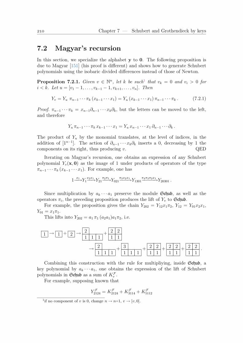
Chapter 7 — Schubert and Grothendieck by keys
7.2 Magyar’s recursionIn this section, we specialize the alphabet y to 0. The following proposition isdue to Magyar [151] (his proof is different) and shows how to generate Schubertpolynomials using the isobaric divided differences instead of those of Newton.
Proposition 7.2.1. Given v ∈ Nn, let k be such1 that vk = 0 and vi > 0 fori < k. Let u = [v1 − 1, . . . , vk−1 − 1, vk+1, . . . , vn]. Then
Yv = Yu πn−1 · · · πk (xk−1 · · ·x1) = Yu (xk−1 · · ·x1) πn−1 · · · πk . (7.2.1)
Proof. πn−1 · · · πk = xn−1∂n−1 · · ·xk∂k, but the letters can be moved to the left,and therefore
Yu πn−1 · · · πk xk−1 · · ·x1 = Yu xn−1 · · ·x1 ∂n−1 · · · ∂k .
The product of Yu by the monomial translates, at the level of indices, in theaddition of [1n−1]. The action of ∂n−1 · · ·xk∂k inserts a 0, decreasing by 1 thecomponents on its right, thus producing v. QED
Iterating on Magyar’s recursion, one obtains an expression of any Schubertpolynomial Yv(x,0) as the image of 1 under products of operators of the typeπn−1 · · · πk (xk−1 · · ·x1). For example, one has
1x1−−→Y1
x2x1−−→Y21π2π1−−→Y021
π3x2x1−−−→Y1301π4π3π2x1−−−−−→Y20301 .
Since multiplication by ak · · · a1 preserve the module Schub, as well as theoperators πi, the preceding proposition produces the lift of Yv to Schub.
For example, the proposition gives the chain Y202 = Y12x1π2, Y12 = Y01x2x1,Y01 = x1π1.
This lifts into Y202 = a1 π1 (a2a1)a1π2, i.e.
1 → 1 + 2 → 2
1 1 1+ 2 2
1 1
→ 2
1 1 1+ 3
1 1 1+ 2 2
1 1+ 2 2
1 1+ 2 2
1 1.
Combining this construction with the rule for multipliying, inside Schub, akey polynomial by ak · · · a1, one obtains the expression of the lift of Schubertpolynomials in Schub as a sum of KFv .
For example, supposing known that
Y F2124 = KF2124 +KF3114 +KF5112
1if no component of v is 0, change n→ n+1, v → [v, 0].

§ 7.2 — Magyar’s recursion
then
Y F2124a2a1 =(KF3224+KF3314+KF5222+KF3512
)+(KF4214+KF5213+KF4511
)+(KF6212+KF6311
)and
Y F32024 = Y F2124π4π3 a2a1 = Y F2124a2a1 π4π3
=(KF32024+KF33014+KF52022+KF35012
)+(KF42014+KF52013+KF45011
)+(KF62012+KF63011
).
To describe in a non-recursive manner the key-decomposition of a Schubertpolynomial, we shall need the nilplactic monoid2.
2 In fact, this application was the original motivation, though not stated, to introduce thenilplactic monoid in [122]. Edelman and Greene’s motivation [34] for the same monoid was toclassify reduced decompositions.

Chapter 7 — Schubert and Grothendieck by keys
7.3 Schubert by nilplactic keysGiven a tableau t which is a reduced decomposition of a permutation ζ, let k be theinteger such that the first column of t is of the type [k, . . . , 1] or [. . . , r, k, . . . , 1],with r > k+1. Let ϕ(t) be the tableau obtained from t (in the nilplactic monoid)by erasing the factor [k, . . . , 1] in the first column of t read by columns. Thenthe code of ζ−1 is of the type [v′ + 1k, 0, v′′], with v ∈ Nk, and ϕ(t) is a reduceddecomposition of σ, the code of σ−1 being [0, v′, v′′]. One can equivalently use thetransposed tableaux and erase in their bottom row a maximal factor of the typei . . . k, i being the minimal letter.
For example, the following tableaux
5
4
2 3 51 2 3 6
→5
42 3 5 6
→ 5
4 5 6→ 5
4 5 6→ 5
are reduced decompositions of the permutations [[3, 6, 2, 1, 5, 7, 4], [1, 3, 6, 2, 5, 7, 4],[1, 2, 3, 6, 5, 7, 4], [1, 2, 3, 6, 5, 7, 4], [1, 2, 3, 4, 6, 5]], whose inverses have respective codes[3, 2, 0, 3, 1], [0, 2, 0, 3, 1], [0, 0, 0, 3, 1], [0, 0, 0, 3, 1], [0, 0, 0, 0, 1].
The following lemma relates the Pieri rule for key polynomials and the recursiveconstruction of tableaux which are reduced decompositions.
Lemma 7.3.1. Let ζ be a permutation of code [v′ + 1k, 0, v′′], and σ be of code[0, v′, v′′]. Let t be a tableau which is a reduced decomposition of σ−1, [0, u] be itskey (as a weight). Let F be the set of tableaux T which are reduced decompositionsof ζ−1 and such that ϕ(T ) = t. Then
Ku x1 . . . xk =∑
T,v=Key(T )
Kv . (7.3.1)
The following theorem, due to [128], shows that the transition between Schu-bert and key polynomials is given by the enumeration of tableaux which are re-duced decompositions.
Theorem 7.3.2. Let σ be a permutation, T (σ) be the set of tableaux which arereduced decompositions of σ−1, K(σ) be the set of their left nilplactic keys (asweights). Then
Xσ(x,0) =∑
u∈K(σ)
Ku . (7.3.2)
Proof. The preceding lemma shows that Magyar’s recursive definition Yv′v′′ →Y[v′+1k,0,v′′] corresponds to the recursion on reduced decompositions which aretableaux. QED
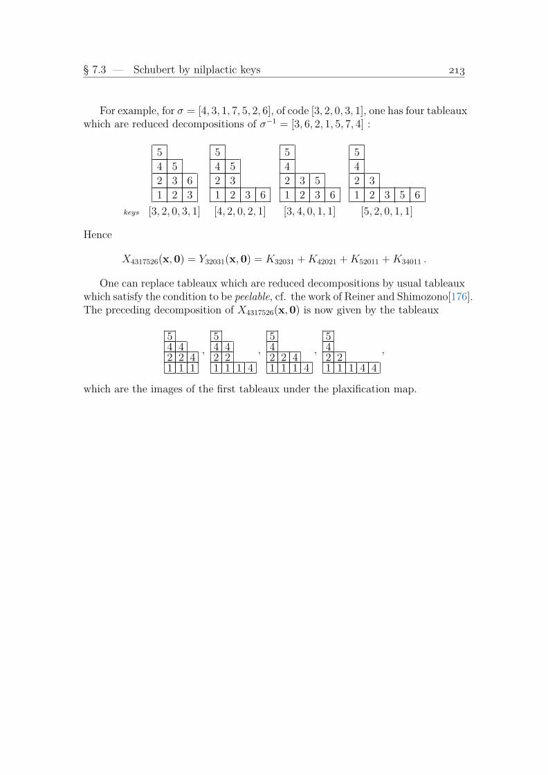
§ 7.3 — Schubert by nilplactic keys
For example, for σ = [4, 3, 1, 7, 5, 2, 6], of code [3, 2, 0, 3, 1], one has four tableauxwhich are reduced decompositions of σ−1 = [3, 6, 2, 1, 5, 7, 4] :
5
4 5
2 3 6
1 2 3
5
4 5
2 3
1 2 3 6
5
4
2 3 5
1 2 3 6
5
4
2 3
1 2 3 5 6
keys [3, 2, 0, 3, 1] [4, 2, 0, 2, 1] [3, 4, 0, 1, 1] [5, 2, 0, 1, 1]
Hence
X4317526(x,0) = Y32031(x,0) = K32031 +K42021 +K52011 +K34011 .
One can replace tableaux which are reduced decompositions by usual tableauxwhich satisfy the condition to be peelable, cf. the work of Reiner and Shimozono[176].The preceding decomposition of X4317526(x,0) is now given by the tableaux
54 42 2 41 1 1
,54 42 21 1 1 4
,542 2 41 1 1 4
,542 21 1 1 4 4
,
which are the images of the first tableaux under the plaxification map.

Chapter 7 — Schubert and Grothendieck by keys
7.4 Schubert by words majorised by reduced de-compositions
Billey, Jockusch, Stanley show in [9] that one can obtain Schubert polynomialsfrom reduced decompositions without using keys.
Given a reduced decomposition sα = sα1 . . . sαr , let R(sα) be the set of weaklydecreasing words w ∈ Nr below α, i.e. such that w1 ≤ α1, . . . , wr ≤ αr, satisfyingthe constraints that αi > αi+1 implies wi > wi+1. Then Billey, Jockusch, Stanleyprove3
Theorem 7.4.1. Let σ be a permutation, sα be the set of reduced decompositionsof σ−1. Then the commutative image in Pol of the sum of all words belonging tothe union of the sets R(sα) is equal to the Schubert polynomial Xσ(x,0).
For example, when σ = [3, 1, 6, 2, 4, 5], then σ−1 = [2, 4, 1, 5, 6, 3] has ninereduced decompositions. Six of them
s1s3s4s5s2, s1s3s2s4s5, s1s3s4s2s5, s3s4s1s5s2, s3s1s4s5s2, s3s1s4s2s5
give empty sets of words. The other three are such that
R(s3s4s5s1s2) = [2, 2, 2, 1, 1], [3, 2, 2, 1, 1], [3, 3, 2, 1, 1], [3, 3, 3, 1, 1]R(s3s4s1s2s5) = [2, 2, 1, 1, 1], [3, 2, 1, 1, 1], [3, 3, 1, 1, 1]
R(s3s1s2s4s5) = [2, 1, 1, 1, 1], [3, 1, 1, 1, 1] ,
and the Schubert polynomial X316245 is indeed equal to x3,2,0 + x2,3,0 + x2,0,3 +x3,0,2 + x2,1,2 + x2,2,1 + x3,1,1 + x4,0,1 + x4,1,0.
Billey-Jockusch-Stanley statement is in fact more precise, the Q-symbol of thereduced decomposition can be used to furnish a sum in the plactic algebra whichis equal to XFσ .
Reiner and Shimozono [174] show that the preceding decomposition can be re-fined, grouping reduced decompositions into nilplactic classes, each of them givingthe key polynomial appearing in the decomposition of the Schubert polynomial.In the preceding case, there are two classes, the class of [3, 4, 5, 1, 2] ∼= [3, 4, 1, 2, 5]which gives
KF203 = 3 31 1 1
+ 2 31 1 1
+ 3 31 1 3
+ 2 31 1 3
+ 2 21 1 3
+ 2 21 1 2
+ 2 21 1 1
and the class of [3, 1, 2, 4, 5] which gives KF401 = 31 1 1 1
+ 21 1 1 1
.
3We reverse words compared to their convention, hence we use reduced decompositions ofthe inverse permutation.

§ 7.5 — Product of a Grothendieck polynomial by a dominant monomial
7.5 Product of a Grothendieck polynomial by adominant monomial
We have described in (4.2.1) products of the type Gσ(x,y)x1 . . . xk by punchingdiagrams. Let us have recourse to softer methods by using the jeu de taquin todescribe more generally the product by a dominant monomial.
The following theorem has been obtained with Fulton [46], and describe prod-ucts in terms of keys. Given a tableau t, denote by yt the monomial image of t byi→ yi.
Theorem 7.5.1. Let σ be a permutation in Sn.
• Let k be an integer, k ≤ n. Then, modulo Sym(xn = yn), one has
G(σ)(x,y)xk . . . x1 ≡∑
u∈U(σ,k)
yuG ’oooooo (E(σ)u)(x,y) . (7.5.1)
Let v ∈ N be the vector of components vn+1−σi = 1 for i = 1, . . . , k, andvn+1−σi = 0 for i = k+1, . . . , n. Then
∑u∈U(σ,k) yu is equal to the key poly-
nomial Kv(yω) in the reversed alphabet yω = [yn, . . . , y1].
• Let λ ∈ Nn be a partition, and v be such that nv1 . . . 1vn be the reordering ofσλ1
1 . . . σλnn . Then
G(σ)(x,y)xλ ≡∑t
ytG ’oooooo (E(σ)t)(x,y) , (7.5.2)
sum over all tableaux of shape λ such that the product E(σ)t be frank. More-over, the sum
∑t yt is equal to the key polynomial Kv(y
ω).
Proof. The first assertion concerns the same case as in (4.2.1). However, insteadof translating punched diagrams in terms of keys, let us rather use the divideddifferences in y−1
1 , y−12 , . . . to prove it by induction.
The starting point is for σ = ω, the assertion resulting in that case fromG(ω)xi ≡ yn+1−iG(ω). Suppose the theorem to be true for the pair σ, k, and let ibe such that `(siσ) ≤ `(σ). Then, according to (2.2.3), one has the recursion
Gsiσ(x,y)xk . . . x1 = Gσ(x,y)xk . . . x1 πy∨
i .
The elements in U(σ, k) are of three types :
• u contains i, i+1 or none of these letters. Then yuG ’oooooo (E(σ)u)πy∨
i = G ’oooooo (E(σ)u)πy∨
i πy∨
i yu.
• pairs of elements u′iu′′ and u′(i+1)u′′. The corresponding subsum is of thetype yu′u′′
(yiGsiζ + yi+1Gζ
), with `(siζ) ≤ `(ζ). Thanks to Leinitz’formula,
this subsum is equal to yu′u′′Gζyiπy∨
i , and therefore invariant under πy∨
i .

Chapter 7 — Schubert and Grothendieck by keys
• elements u = u′(i+1)u′′, such that i 6∈ u′′ and u′iu′′ 6∈ U(σ, k). In that case,ζ = ’oooooo (E(σ)u) is such that `(siζ) ≤ `(ζ), and
Gζ yuπy∨
i = Gζπy∨
i ysiu +Gζ yu = Gsiζ ysiu +Gζyu .
In total, U(siσ, k)\U(σ, k) is the image under the exchange of i, i+1 of the elementsof the third type, and for those elements, one has siζ = ’oooooo (E(siσ)(siu)) andζ = ’oooooo (E(siσ)u). Hence the summation (7.5.1) is still valid for siσ.
Moreover, when w ∈ 0, 1n, the element KFw is the sum of all columns ma-jorized by a fixed column, and its image under the involution u → ω uω is thesum of all columns which majorize a given column. The commutative evaluationof this last element is therefore a key polynomial on a reversed alphabet and onechecks that the index corresponding to σ, k is the one stated.
The second part of the theorem results from the associativity of keys: ’oooooo (tt′) =’oooooo
(E(
’oooooo (t))t′). QED
For example of (7.5.2), let σ = [4, 1, 3, 5, 2] and λ = [2, 1, 1]. Then 4211315020
reorders into 5042312011, so that v = [0, 2, 1, 0, 1], and one has to enumerate thetableaux in KF02101, which are
321 1
,321 2
,421 1
,421 2
,431 1
,431 2
,432 2
,521 1
,521 2
,531 1
,531 2
,532 2
One then has to take the images of these tableaux under t → ω tω, and thisfurnishes the following value of G(41352)(x,y)x21100, writing the tableaux t insteadof the monomials yt :
G(41352)x21100 =
5
4
1 5
G(51432) +5
4
2 4
G(42531) +5
4
3 4
G(43512) +5
3
2 5
G(52341)
+5
4
1 4
G(41532) +5
4
3 5
G(53412) +4
3
2 4
G(42351) +4
3
1 5
G(51342)
+4
3
2 5
G(52341) +5
4
2 5
G(52431) +5
3
1 5
G(51342) +4
3
1 4
G(41352) .
Notice that the product
K41352x211 = K62452 +K72442 +K62632 +K72532
+K64612 +K74512 +K63451 +K73441 +K63631 +K73531

§ 7.5 — Product of a Grothendieck polynomial by a dominant monomial
has only 10 terms, and thus does not allow to describe the productG(41352)(x,y)x21100.Indeed, according to (4.4.1), one has to take parts differing by at least 2 = λ1 torelate the two products. The weight 2× [4, 1, 3, 5, 2] = [8, 2, 6, 10, 4] is appropriate,the product
K8,2,6,10,4x211 = K10,3,7,10,4 +K11,3,7,9,4 +K12,3,7,8,4 +K10,3,11,6,4 +K12,3,9,6,4
+K10,7,11,2,4+K12,7,9,2,4+K10,5,7,10,2+K11,5,7,9,2+K12,5,7,8,2+K10,5,11,6,2+K12,5,9,6,2
has 12 terms from which one reads the 12 permutations occurring in the productG(41352)(x,y)x21100.

Chapter 7 — Schubert and Grothendieck by keys
7.6 ASM and monotone trianglesWe have already met a correspondence between Grothendieck polynomials andkey polynomials when describing the multiplication by x1 · · ·xk. In fact, thiscorrespondence was a direct consequence of the commutation relations betweenthe πi’s and the xi’s.
We describe now a more subtle correspondence, by putting an appropriateweight on staircase tableaux. The tableaux which have a non-zero weight are thetableaux of staircase shape which do not contain a subtableau of the type b
a c,
with c ≥ b.Equivalently, they are the tableaux of staircase shape with weakly decreasing
diagonals, which appear in the literature as monotone triangles. These tableauxare in (easy) bijection with alternating sign matrices (ASM), but tableaux will fitbetter in this text.
Let us define a weight on tableaux, as a product of elementary weights ontableaux of shape [1, 2]. The weight of a subtableau of shape [1, 2] on columnsj−1, j and consecutive rows is, for three integers a < b < c,
ca b
cb b
cb c
ba c
ϕG weight yjx−1b yjx
−1b − 1 1 0
.
By definition, the weight ϕG(T ) of a staircase tableau T is the product of theseelementary weights, on all subtriangles. The image of ϕG(T ) under the changeof variables xi → (1−xi)
−1, yj → (1−yj)−1 is denoted ϕ
eG(T ). Explicitely, theelementary weights are now
ca b
cb b
cb c
ba c
ϕeG weight (xb−1)(yj−1)−1 (xb−yj)(yj−1)−1 1 0
.
For example, pointing out the rightmost box of the elementary tableaux con-
tributing to the weight, the tableau t =42 31 1 2
has weight
4
2 3
1 1 2
→ ϕG(t) =
•• y1x
−13
• y1x−11 −1 y2x
−12
→ ϕeG(t) =
•• x3−1
y1−1
• x1−y1y1−1
x2−1y2−1
.
The following property is proved4 in [103], by checking its compatibility withtransitions. It states that any Grothendieck polynomial is obtained by enumerat-ing all the monotone triangles having a fixed right key, or, equivalently, because
4Keys can be defined directly on ASM. For the correspondence with the keys (of tableaux)that we use here, see Aval [2].

§ 7.6 — ASM and monotone triangles
the non-monotone tableaux have weight 0, enumerating all the tableaux in someKFσ .
Theorem 7.6.1. Let σ ∈ Sn. Then
(−1)`(σ)G(σ)(x,y) =∑
T∈ bKFσ ϕG(T ) , (7.6.1)
(−1)`(σ)G(σ)(x,y) =∑
T∈ bKFσ ϕeG(T ) . (7.6.2)
For example, for σ = [4, 2, 1, 5, 3], there are fifteen tableaux in KFσ . Only 4 ofthem are monotone triangles, and their respective ϕG weights are
54 53 4 52 2 2 41 1 1 1 4
y3x4
( y1x2−1)( y2
x2−1)( y1
x1−1)( y2
x1−1)( y3
x1−1)
54 53 3 52 2 2 41 1 1 1 4
y3x4
( y1x3−1)( y1
x2−1)( y2
x2−1)( y1
x1−1)( y2
x1−1)( y3
x1−1)
54 53 4 52 2 4 41 1 1 1 4
( y1x2−1)( y3
x4−1)( y1
x1−1)( y2
x1−1)( y3
x1−1)
54 53 3 52 2 3 41 1 1 1 4
y3x4
( y1x3−1)( y1
x2−1)( y1
x1−1)( y2
x1−1)( y3
x1−1)
Therefore, the Grothendieck polynomial G(42153) is equal to
G(42153)(x,y) = G3101(x,y) = (1−y1
x2
)(1−y1
x1
)(1−y2
x1
)(1−y3
x1
)(1−y1y2y3
x2x3x4
) ,
while the ϕ eG-weight of the same four tableaux furnishes
G3101(x,y) =(x2 − y1) (x1 − y3) (x1 − y2) (x1 − y1)
(1− y1)3 (1− y3)2 (1− y2)2 (−y2y3y1 + y2y3 + y1y2
− y2 + y3y1 − y3 − y1 − x4x3 + x4 + x4x2x3 − x4x2 + x3 − x3x2 + x2) .
Theorem 5.1.9 gives for this polynomial the expression
G3101(xy) =Y3101(x,y)
(1−y2 − 1) (1−y3)2 (1−y1)2 −Y3111(x,y)
(1−y2) (1−y1)3 (1−y3)2
− Y3201(x,y)
(1−y1)2 (1−y3)2 (1−y2)2 +Y3211(x,y)
(1−y1)3 (1−y3)2 (1−y2)2 .

Chapter 7 — Schubert and Grothendieck by keys
The specialisation z = 0 of (2.9.6) gives the value of the alternating sum ofGrothendieck polynomials, which is also the sum of the weights of all monotonetriangles : ∑
T∈KFn...1
ϕG(T ) =∑σ∈Sn
(−1)`(σ)G(σ)(x,y) = yρx−ρ . (7.6.3)
The specialisation x = 1 of this last formula is due to Bousquet-Mélou & Habsieger[13].

Chapter 8Generating Functions
8.1 Binary trianglesOne can interpret the Cauchy formula for Schubert and Grothendieck polynomialsin many different ways, the Cauchy kernel itself may be thought as the generatingfunction of the Schubert and Grothendieck basis. To generalize this kernel intoan element of a non-commmutative algebra, one uses planar displays.
Expanding a planar object with n boxes containing a sum a + b of elementsbelonging to two families means enumerating the 2n pairs of complementary ob-jects obtained by choosing either a or b in each box. For example, the expansion
of+
+ ++
is equal to
(
,·· ··
)+( ·
,· ··
)(
,·· ··
)+(·
,·
··
)+ · · ·+
( ·· ·,
·
)( ·· ·,
·
)+( ·· ··,
),
writing a sum instead of a set of pairs. Each pair can afterwards be read in aprecise manner so as to furnish a pair of words.
We shall essentially use planar objects of triangular shape. Decomposing a
triangle ++ +
can be thought as enumerating binary triangles (i.e. each
box is filled with either 0 or 1) of a fixed shape. In other words, the set
11 1
, 01 1
, 10 1
, 11 0
, 00 1
, 01 0
, 10 0
, 00 0
codes the same information as the set of pairs(
,
),
(
,
), . . . ,
(
,
)221

Chapter 8 — Generating Functions
used previously.In the following of this chapter, we shall enumerate binary triangles and put
various weights on them.

§ 8.2 — Generating function in the nilplactic algebra
8.2 Generating function in the nilplactic algebraLet us first use the nilplactic algebra with generators v1, v2, . . . , vn−1 satisfying
v2i = 0 , vivi+1vi = vi+1vivi+1 (8.2.1)
vjvivk = vjvkvi , vivkvj = vkvivj (i < j < k) (8.2.2)
Given a commutative alphabet xn, define the nilplactic kernel ΘNlP(xn) to be
ΘNlP(xn) :=
(1 + x1vn−1)(1 + x1vn−2) (1 + x2vn−1)
... ...(1 + x1v1) (1 + x2v2) · · · (1 + xn−1vn−1)
,
reading the kernel by columns (downwards) from left to right.One still has a crystal structure on the terms in the expansion of ΘNlP(xn), as
we had in the plactic case (cf. ??).
EXEMPLE
Given a tableau T in v1, v2, . . . , which is a reduced decomposition, denote byB(T ) ∈ Nn its bottom key (as a weight). Then an analysis of the nilplactic stringssimilar to the one performed in ?? gives the following expansion.
Theorem 8.2.1. Given n, the nilplactic kernel expands in the nilplactic algebraas
ΘNlP(xn) ∼=∑T
KB(T ) T ,
sum over all tableaux which are reduced decompositions of permutations of Sn.
For example, for n = 4, there are 25 tableaux (all permutations, except[2, 1, 4, 3], have only one tableau as a reduced decomposition), and ΘNlP(x4) isequal to
K0 +K1 1 +K01 2 +K001 3 +K11 1 2 +K101 1 3 +K0232
+K221
+K231
+K011 2 3 +K1231 2
+K3
321
+K20121 3
+K2121 2
+K02132 3
+K111 1 2 3 +K21121 2 3
+K222 31 2
+K301
321 3
+K31
321 2
+K12131 2 3
+K2212 31 2 3
+K311
321 2 3
+K32
32 31 2
+K321
32 31 2 3
.
All key polynomials Ku of index u ≤ ρ occur in the expansion of ΘNlP(xn),but with eventual multiplicities (in the example above, K2 occurs twice).

Chapter 8 — Generating Functions
8.3 Generating function in the NilCoxeter alge-bra
By projecting the nilplactic algebra to the NilCoxeter algebra, one obtains a gen-erating function where blocks correspond to all the tableaux which are reducedof the same permutation. In fact, this projection gives back the expansion ofSchubert polynomials Xσ(x,0) in terms of keys seen in (7.3.2)1.
To recover Schubert polynomials in two alphabets, let us take three alphabetsx,y, z and define
Θ∂n(x,y) =
1+(x1−yn−1)∂zn−1
1+(x1−yn−2)∂zn−2 1+(x2−yn−2)∂zn−1... ...
1+(x1−y1)∂z1 1+(x2−y1)∂z2 . . . 1+(xn−1−y1)∂zn−1
.
The expansion of such kernel is equal to a sum∑
σ∈Sncσ(x,y)∂zσ that one can
determine by making it act on the monomial zn−1,...,1,0, but we shall rather takethe function Xω(zω,y). Indeed, we have already made this computation in (1.7.2),up to minor changes including a reversal of alphabet. One has obtained, say forn = 4, the identity (reading the display by columns)
z4−y1 z4−y2 z4−y3
z3−y1 z3−y2
z2−y1
1+(x1−y3)∂z3
1+(x1−y2)∂z2 1+(x2−y2)∂z3
1+(x1−y1)∂z1 1+(x1−y2)∂z3 1+(x1−y3)∂z3
=
z4−x3 z4−x2 z4−x1
z3−x2 z3−x1
z2−x1
,
using only that
(zi+1 − y)(1 + (x− y)∂zi )) = (zi+1 − y)− (x− y) = zi+1 − x .
More generally, for any n, one has
Xω(zω,y) Θ∂n(x,y) = Xω(zω,x) . (8.3.1)
Using the Cauchy formula
Xω(zω,x) =∑σ∈Sn
Xσ−1(y,x)Xσω(zω,y) ,
1left and bottom keys are exchanged, because one takes the reduced decompositions of σ inone case, and of σ−1 in the other.

§ 8.4 — Generating function in the NilCoxeter algebra
and comparing with
Xω(zω,y)cσ(x,y)∂zσ =∑
(−1)`(σ)cσ(x,y)Xω(ωσω)(zω,y) ,
one finds thatcσ(x,y) = (−1)`(σ)Xσ−1(y,x) = Xσ(x,y) .
In final, one has obtained that Θ∂n(x,y) is a generating function of Schubert
polynomials.
Theorem 8.3.1. Let n be a positive integer. Then
Θ∂n(x,y) =
∑σ∈Sn
Xσ(x,y) ∂zσ . (8.3.2)
For example, for σ = [3, 1, 5, 2, 4], there are 5 configurations which contributeto X31524(x,y). Grouping reduced decompositions according to their nilplacticclass, one has
X31524(x,y) =
x1−y4
• •x1−y2 x2−y2 •x1−y1 • • •
+
x1−y4
• •x1−y2 • •x1−y1 • x3−y1 •
421 3
+
•• x2−y3
x1−y2 x2−y2 •x1−y1 • • •
+
•• x2−y3
x1−y2 • •x1−y1 • x3−y1 •
+
•• •
x1−y2 • x3−y2
x1−y1 • x3−y1 •
2 41 3
.
This theorem is given by Fomin and Kirillov in [39, 38], and is also a corollaryof the Hopf decomposition of Schubert polynomials given in [122].
The proof of Fomin and Kirillov is very simple, it consists in noticing thatΘ∂n∂
zi = Θ∂
n∂i. This property instantly allows to characterize the behaviour ofcoefficients with respect to the divided differences in x, and to recognize these co-efficients to be Schubert polynomials. We have already several times encounteredcases where the action of divided differences is exchanged with another operation(which is here, multiplication in the algebra generated by the ∂zi ’s).
The Cauchy formula (2.10.2) translates into the following multiplicative prop-erty of generating functions
Θ∂(x,y) = Θ∂(u,y) Θ∂(x,u) , (8.3.3)
that Fomin and Kirillov prove directly by using the Yang-Baxter equation.

Chapter 8 — Generating Functions
8.4 Generating function in the 0-Hecke algebraThe preceding considerations can easily be adapted to the Grothendieck world.This time, one has to use the 0-Hecke algebra, with generators πz1, . . . , πzn−1, in-stead of the 00-Hecke algebra (NilCoxeter algebra).
Let
Θbπn(x,y) =
1+(1−yn−1
x1)πzn−1
1+(1−yn−2
x1)πzn−2 1+(1−yn−2
x2)πzn−1
... ...1+(1− y1
x1)πz1 1+(1− y1
x2)πz2 . . . 1+(1− y1
xn−1)πzn−1
.
Using that (1− zi+1
y
)(1 + (1− y
xπzi ))
= 1− zi+1
x,
starting with ΘG(z,y) =∏
1≤i<j≤n(1− zjy−1i ), one obtains
ΘG(z,y)Θbπn = ΘG(z,x) . (8.4.1)
Comparing with the Cauchy formula (2.9.4), one obtains the following generatingfunction of Grothendieck polynomials.
Theorem 8.4.1. Let n be a positive integer. Then
Θbπn(x,y) =
∑σ∈Sn
G(σ)(x,y) πzσ . (8.4.2)
For example, for n = 3, one has
1 + (1−y2x−11 )πz2
1 + (1−y1x−11 )πz1 1 + (1−y1x
−12 )πz2
= 1 + (1−y1x−11 )πz1 + (1−y1y2(x1x2)−1)πz2 + (1−y1x
−11 )(1−y1x
−12 )πz1π
z2
+ (1−y2x−11 )(1−y1x
−11 )πz2π
z1 + (1−y2x
−11 )(1−y1x
−11 )(1−y1x
−12 )πz2π
z1π
z2
= 1 +G(213)πz1 +G(132)π
z2 +G(231)π
z231 +G(312)π
z312 +G(321)π
z321 .
This generating function has been obtained by Fomin and Kirillov in [38], butis also a corollary of the Hopf decomposition of Grothendieck polynomials givenin [122].
The generating function Θbπn(x,y) of G-polynomials is obtained by taking a
kernel with factors of the type (xi − yj)(1 − yj)−1 instead of 1 − yjx
−1i . For
example,(1 +
x1−y2
1−y2
πz2
)(1 +
x1−y1
1−y2
πz1
)(1 +
x2−y1
1−y1
πz2
)=∑σ∈S3
G(σ)(x,y) πzσ

§ 8.5 — Hopf decomposition of Schubert and Grothendieck polynomials
8.5 Hopf decomposition of Schubert and Groth-endieck polynomials
Any polynomial in x1, . . . , xn can be filtered according to the powers of x1. Inother words, one can use that Pol(xn) ' Pol(x1) ⊗Pol(x2, . . . , xn) and compareexpansions in the natural bases of the two spaces.
In the case of symmetric functions, the isomorphism
Sym(xn) ' Sym(x1)⊗Sym(x2, . . . , xn)
reveals the existence of a Hopf structure on Sym(xn). I kept the same terminol-ogy with M.P. Schützenberger for what concerns polynomials in the Schubert orGrothendieck bases. In the case of Macdonald polynomials, one filters accordingto xn instead.
From the generating functions (8.3.2) and (8.4.2) one deduces the followingHopf decompositions given in [122].
Theorem 8.5.1. Let σ be a permutation in Sn, v be its code, x+ = x2, . . . , xn.Then
Yv(xn,0) =∑w∂ ,u
x|v|−|u|1 Yu(x
+,0) , (8.5.1)
sum over all words w∂ in the expansion of (1+∂n−1) · · · (1+∂1), all u ≤ [n−2, . . . , 0]such that ∂σ = w∂∂ζ, with ζ of code [0, u].
Similarly
Gv(xn,0) =∑wbπ ,u
(−1)|u|+`(wbπ−|v|x|u|+`(wbπ)1 Gu(x
+,0) (8.5.2)
G1/xv (xn,1) =
∑wbπ ,u
(−1)|u|+`(wbπ−|v|)(1−x1)|u|+`(wbπ)G1/xu (x+,1) (8.5.3)
sum over all words wbπ in the expansion of (1+πn−1) · · · (1+π1), all u ≤ [n−2, . . . , 0]such that πσ = ±wππζ, with ζ of code [0, u].
Statements (8.5.1) and (8.5.2) are strictly equivalent to (8.3.2) and (8.4.2)(adding the second alphabet y is no problem), though, we agree, much less elegant.
The two expansions (8.5.1) and (8.5.2) involve the same set u, but in thesecond case, each u may correspond to several words wbπ. For example, figuringthe words in the expansion, one has
Y021(x,0) = Y21(x+,0)+(x1∂2)Y20(x+,0)+(x1∂3)Y11(x+,0)+(x21∂3∂2)Y01(x+,0) ,
G021(x,0) = (1−x1π3−x1π2+x21π3π2)G21(x+,0) + (x1π2−x
21π3π2)G20(x+,0)
+ (x1π3−x21π3π2)G11(x+,0) + (x2
1π3π2)G01(x+,0) ,

Chapter 8 — Generating Functions
the final expansion being
G021(x,0) = (1−x1)2G21(x+,0) + x1(1−x1)G20(x+,0)
+ x1(1−x1)G11(x+,0) + x21G01(x+,0) .
For a given pair v, u, one checks that, keeping only the terms contributingto the Hopf decomposition, the product (1+x1πn−1) · · · (1+x1π1) simplifies into aproduct of factors of the type 1, x1πj or 1+x1πj. Therefore, the total coefficientof Gu(x
+,0) is equal to some power of x1 multiplied by a power of (1−x1). Thus,Example 2.6 of [122] reads
G14101(x,0) = a14G1101(x+,0) + a1
3b1G2101(x+,0) + a12b1G41(x+,0)
+ a12b1G3101(x+,0) + a1b1
2G4101(x+,0) ,
putting ai = xi, bi = 1−xi.Iterating the Hopf decomposition, one obtains an expression of Gv(x,0) as a
positive polynomial in a1, b1, a2, b2, . . . . Interchanging a and b gives the expressionof G1/x
v (x,1) .For example,
G202(x,0) = a3a2b2b1a12 + a3b2a1
3 + a22b1a1
2 + a2a13 + b2b1a1
2a32
G1/x202 (x,1) = b3b2a2a1b1
2 + b3a2b13 + b2
2a1b12 + b2b1
3 + a2a1b12b3
2 .
Notice that the specialization bi = 1 in the expression of Gv(x,0) gives the Schu-bert polynomial Yv(x,0). We have not investigated the properties of these poly-nomials.

§ 8.6 — Generating function of G-polynomials
8.6 Generating function of G-polynomialsWe shall use simultaneoulsy several weights on 0−1 triangles T of shape [1, . . . , n−1]: A triangle T gives rise to a monomial φx(T ), a product φy(T ) of factors −yi, aproduct φπ(T ) of πi’s and a product φ∂(T ) if ∂i’s, as follows :
φx(T ) =∏
x1−Tiji
φy(T ) =∏
(−yi)1−Tij & φy−1(T ) =
∏(1−yi)
1−Tij
φπ(T ) =∏
πTijn−i+j−1
φ∂(T ) =∏
∂1−Tijn−i ,
reading the successive columns from left to right for φπ(T ), and reading by suc-cessive rows, each row from right to left, for φ∂(T ) (we use matrix coordinates).
Reading order
12 43 5 6
filling
π3
π2 π3
π1 π2 π3
for φπ ,
13 26 5 4∂3
∂3 ∂2
∂3 ∂2 ∂1
for φ∂ .
For example, one has
for T =0
1 0
0 1 1
,•π2 •• π2 π3
&∂3
• ∂2
∂3 • •
Φπ(T ) = π2π2π3 Φ∂(T ) = ∂3∂2∂3
,
x3
• x2
x1 • •⇒ Φx(T ) = x3x2x1 & Φy(T ) = (1−y3)(1−y2)(1−y1) .
Let ζ(T ) be the permutation such that φπ(T ) = πζ , and σ(T ) be the permu-tation such that φ∂(T ) = ∂σ (if φ∂(T ) is not 0).
Theorem 8.6.1. Given n and ζ, σ ∈ Sn, let T (σ) be the set of 0-1 triangles suchthat σ(T ) = σ. Then
Xσ(x,y) =∑
T∈T (σ)
φy(T ) G(ζω)(x,y) (8.6.1)
Xσ−1(x,0) =∑
T∈T (σ)
φx(T ) . (8.6.2)
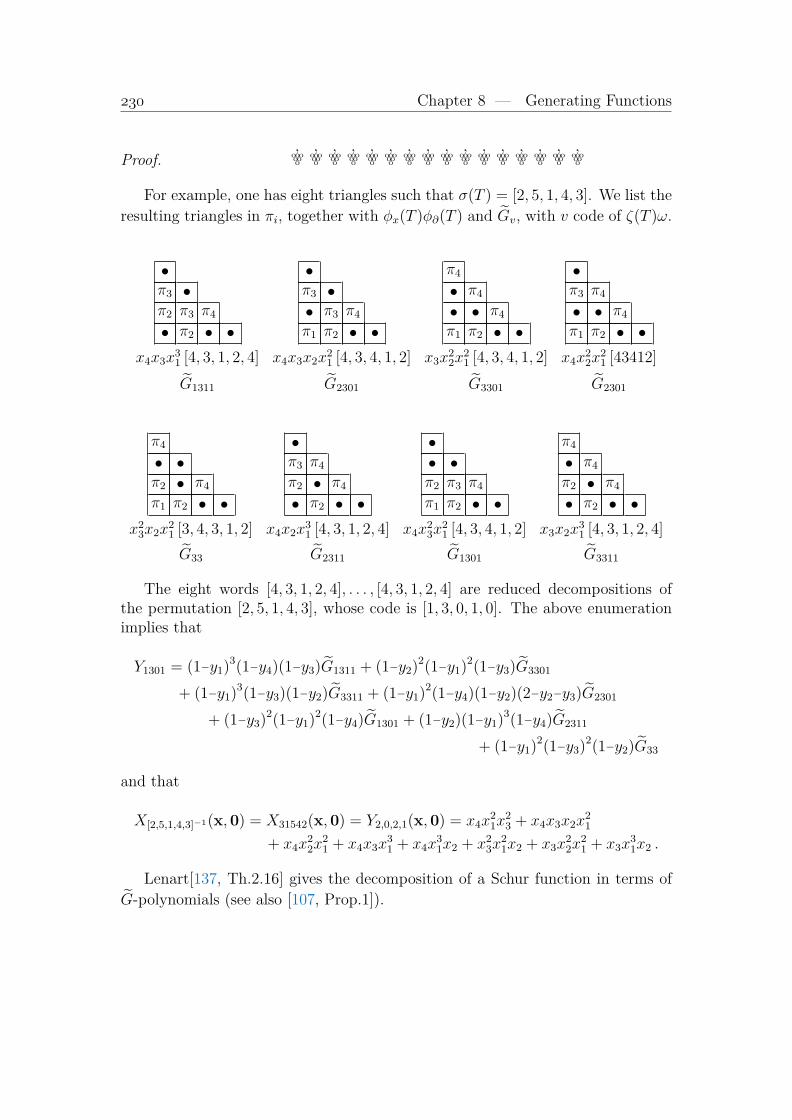
Chapter 8 — Generating Functions
Proof. ’oooooo’oooooo
’oooooo’oooooo
’oooooo’oooooo
’oooooo’oooooo
’oooooo’oooooo
’oooooo’oooooo
’oooooo’oooooo
’oooooo’oooooo
For example, one has eight triangles such that σ(T ) = [2, 5, 1, 4, 3]. We list theresulting triangles in πi, together with φx(T )φ∂(T ) and Gv, with v code of ζ(T )ω.
•π3 •π2 π3 π4
• π2 • •
•π3 •• π3 π4
π1 π2 • •
π4
• π4
• • π4
π1 π2 • •
•π3 π4
• • π4
π1 π2 • •x4x3x
31 [4, 3, 1, 2, 4] x4x3x2x
21 [4, 3, 4, 1, 2] x3x
22x
21 [4, 3, 4, 1, 2] x4x
22x
21 [43412]
G1311 G2301 G3301 G2301
π4
• •π2 • π4
π1 π2 • •
•π3 π4
π2 • π4
• π2 • •
•• •π2 π3 π4
π1 π2 • •
π4
• π4
π2 • π4
• π2 • •x2
3x2x21 [3, 4, 3, 1, 2] x4x2x
31 [4, 3, 1, 2, 4] x4x
23x
21 [4, 3, 4, 1, 2] x3x2x
31 [4, 3, 1, 2, 4]
G33 G2311 G1301 G3311
The eight words [4, 3, 1, 2, 4], . . . , [4, 3, 1, 2, 4] are reduced decompositions ofthe permutation [2, 5, 1, 4, 3], whose code is [1, 3, 0, 1, 0]. The above enumerationimplies that
Y1301 = (1−y1)3(1−y4)(1−y3)G1311 + (1−y2)2(1−y1)2(1−y3)G3301
+ (1−y1)3(1−y3)(1−y2)G3311 + (1−y1)2(1−y4)(1−y2)(2−y2−y3)G2301
+ (1−y3)2(1−y1)2(1−y4)G1301 + (1−y2)(1−y1)3(1−y4)G2311
+ (1−y1)2(1−y3)2(1−y2)G33
and that
X[2,5,1,4,3]−1(x,0) = X31542(x,0) = Y2,0,2,1(x,0) = x4x21x
23 + x4x3x2x
21
+ x4x22x
21 + x4x3x
31 + x4x
31x2 + x2
3x21x2 + x3x
22x
21 + x3x
31x2 .
Lenart[137, Th.2.16] gives the decomposition of a Schur function in terms ofG-polynomials (see also [107, Prop.1]).

Chapter 9Key polynomials for type B,C,D
9.1 KB, KC, KD
For each type ♥ = B,C,D, we are going to define two families of key polynomials,indexed by elements of Zn, using the divided differences π♥i or π♥i , and modifyingthe indices using s♥i .
In more details, in type ♥ = B,C, we start with all dominant monomialsxv : v1 ≥ · · · ≥ vn ≥ 0 and put
xv = K♥v = K♥v .
The other polynomials are defined recursively by
K♥v πi = K♥v si & K♥v πi = K♥v si , when vi > vi+1 , i < n , (9.1.1)
K♥v π♥n = K♥
v s♥n& K♥v π
♥n = K♥
v s♥n, when vn > 0 , for ♥ = B,C . (9.1.2)
In type D, we would not obtain enough elements to span the space of poly-nomials. To the set of dominant monomials xv used in types A,B,C, we haveto add all xu, with u = [v1, . . . , vn−1,−vn]. In short, let us call D-dominant thevectors [v1, . . . , vn−1,±vn], v1 ≥ · · · ≥ vn ≥ 0.
We start with
xv = KDv = KD
v when v is D-dominant
and define recursively the other polynomials by
KDv πi = KD
v si& KD
v πi = KDv si
, when vi > vi+1 , i < n , (9.1.3)
KDv π
Dn = KD
v sDn& KD
v πDn = KD
v sDn, vn−1 + vn > 0 . (9.1.4)
The definition is consistent since the operators satisfy the braid relations, andsince the hypotheses used in the recursive steps insure that length increase.
231

Chapter 9 — Key polynomials for type B,C,D
Notice that, when v ∈ Nn, then all K♥v (resp. K♥v ), ♥ = A,B,C,D coincidewith each other, since the exceptional generators sBn or sDn are not used.
On vectors in Zn, put the following lexicographic order : u >L v if there existsi : u1 = v1, . . . , ui−1 = vi−1 and ui < vi. From the explicit action of the divideddifferences, one sees that each K♥v , K♥v has dominant term xv. In fact, one hasused the operators π♥i (resp. π♥i ) to generate the polynomials K♥v (resp. hK♥v ),and the action of s♥i on the indices of the key polynomials. Therefore, one has thefollowing theorem.
Theorem 9.1.1. The sets K♥v : v ∈ Zn, K♥v : v ∈ Zn constitute six basesof Pol(x±n ), which are triangular in the basis of monomials with respect to thelexicographic order.
For example,
KB−1,−2,1 = x−1,−2,1 + x−1,−1,0 + x−1,−1,1 + x−1,0,−1 + x−1,0,0 + x−1,0,1 + x0,−2,0
+ x0,−2,1 + x0,−1,−1 + 2x0,−1,0 + 2x0,−1,1 + x0,0,−1 + 2x0,0,0 + x0,0,1 ,
KC−1,−2,1 = x−1,−2,1 +x−1,−1,0 +x−1,0,−1 +x−1,0,1 +x0,−2,0 +x0,−1,−1 +x0,−1,1 +x0,0,0 ,
KD−1,−2,1 = x−1,−2,1 + x−1,−1,0 + x−1,0,−1 + x0,−2,0 + x0,−1,−1 + x0,−1,1 + x0,0,0 .
To my knowledge, the relations between the bases for different types have notbeen investigated. Continuing with the preceding example, one has
KB−1,−2,1 = KC
−1,−2,1 + KC−1,−1,1 + KC
0,−2,1 + KC0,−1,1
= KD−1,−2,1 + KD
−1,−1,1 + KD−1,0,1 + KD
0,−2,1 + KD0,−1,1
KC−1,−2,1 = KB
−1,−2,1 − KB−1,−1,1 + KB
−1,0,1 − KB0,−2,1 + KB
0,−1,1
= KD−1,−2,1 + KD
−1,0,1
KD−1,−2,1 = KB
−1,−2,1 − KB−1,−1,1 − KB
0,−2,1 + KB0,−1,1
= KC−1,−2,1 − KC
−1,0,1 .
On the other hand, for a given type ♥, the relations between K♥ and K♥ aregiven by the Bruhat order1, thanks to Lemma 1.10.4.
Lemma 9.1.2. For any type ♥, given any weight v, one has the following relation
K♥v =∑u≤v
K♥u (9.1.5)
1One defines the ♥-Bruhat order on elements of Zn which are in the orbit of a dominantweight, by generating the elements of the orbit by successive application of simple transpositions.For example, for n = 3, type B or C, one has the chain x321 < x312 < x312 < x321 < · · · . Thelength is also defined as the minimum length of a sequence of simple transpositions which reorderthe weight into a dominant weight. Notice that to order the elements of the group, wich aredenoted by the same vectors, one uses the same “Hasse diagram”, but starts with [1, 2, 3] insteadof [3, 2, 1].

§ 9.1 — KB, KC , KD
For example,
KB0,−2,0 = KB
0,−2,0 + KB0,0,−2 + KB
0,0,2 + KB0,2,0 + KB
2,0,0 ,
butKB
0,−2,0 = KB0,−2,0 −KB
0,0,−2 .
The full Bruhat interval does not occur in the second formula, because the Moëbiusfunction takes values in 0, 1, −1 in the case of the orbit of [2, 0, 0], contrary to thecase of the orbit of [3, 2, 1], which is the case of the group itself (Lemma 1.10.4).

Chapter 9 — Key polynomials for type B,C,D
9.2 Scalar products for type B,C,DLet ∆♥ be the denominator of Weyl character formula. Weyl defined a scalarproduct on characters by taking a constant term involving the square of ∆♥. Thisis not appropriate in the case of key polynomials, because they are not invariantunder the associated group, contrary to characters. As in the case of the non-symmetric Cauchy kernel, the solution is to take only half of the factors of thesymmetric kernel, here, to take only ∆♥.
Definition 9.2.1. Let ρB = [n− 12, . . . , 2− 1
2, 1− 1
2], ρC = [n, . . . , 2, 1], ρD = ρA =
[n−1, . . . , 1, 0]. For ♥ = B,C,D let
Ω♥ = xρ♥
∆♥ .
Let moreover ε = (−1)n when ♥ = B,C, and ε = 1 when ♥ = D. Then for anypair of Laurent polynomials f, g in x1, . . . , xn, define
(f, g)♥ = CT(ε fg xρ
♥∆♥). (9.2.1)
For example, taking n = 2, one has
(f, g)B = CT(fgx
3/21 x
1/22 (x
1/21 − x−1/2
1 )(x1/22 − x−1/2
2 )(x1 − x2)(1− 1
x1x2
))
= CT(fg (1− x1)(1− x2)(1− x1/x2)(1− x1x2)
),
(f, g)C = CT
(fg x2
1x2 (x1 −1
x1
)(x2 −1
x2
)(x1 − x2)(1− 1
x1x2
)
),
= CT(fg (1− x2
1)(1− x22)(1− x1/x2)(1− x1x2)
),
(f, g)D = CT(fg x1 (x1 − x2)(1− 1
x1x2
))
= CT(fg (1− x1/x2)(1− x1x2)
).
In the language of root systems, the different kernels are products over all thepositive roots.
To define the scalar product ( , )♥, one could as well give the finite list of allmonomials xv such that (xv , 1)♥ 6= 0.
For example, for type C2, we need only the list (xv, 1)C = 1 for v = [0, 0], [−1,−3], [−3, 1], [−4,−2],and (xv, 1)C = −1 for v = [0,−2], [−1, 1], [−3,−3], [−4, 0].
In fact, the scalar product ( , )♥ is related to the maximal symmetrizer π♥w0, as
shows the next property.
Lemma 9.2.2. Let ♥ = B,C,D. Then (xv, 1)♥ takes values in 0, 1, −1. Thekernel Ω♥n expands as
Ω♥n =∑v∈Zn
(xv, 1)♥x−v .
Moreover, xvπ♥w0= ±1 if and only if xvπ♥w0
= (xv, 1)♥.

§ 9.2 — Scalar products for type B,C,D
Proof. That x−v occurs with multiplicity c in the expansion of xρ♥∆♥ is is anotherway of stating that (xv, 1)♥ = c. This proves the first statement.
The ♥-Vandermonde expands as a sum∑
u±xu, over all signed permutationsof ρ♥. Therefore, x−v occurs in the expansion of Ω♥ if and only if v + ρ♥ is asigned permutation of ρ♥. On the other hand, for any v, xvπ♥w0
is equal to 0, orthere exists a dominant weight λ such that xvπ♥w0
= ±xλπ♥w0. This last function
is equal to ±1 if and only if λ = [0, . . . , 0], which exactly means that v + ρ♥ is asigned permutation of ρ♥. QED
The crucial property of the scalar products ( , )♥ is their compatibility withthe operators generating the key polynomials.
Proposition 9.2.3. Write πn = π♥n , πn = π♥n , for ♥ = B,C,D. Then theoperators πi and πi (1 ≤ i ≤ n) are self-adjoint with respect to ( , )♥, i.e. forevery pair of Laurent polynomials f, g, one has(
fπi , g)♥
=(f , gπi
)♥,(fπi , g
)♥=(f , gπi
)♥.
Proof. For i = 1, . . . , n−1, the proof is similar to the case of type A, except that westart with fg instead of f(x1, . . . , xn)g(x−1
n , . . . , x−11 ). In the case i = n, ♥ = B,C,
one first computes the constant term with respect to xn and writes
(f , g)♥ = CT(CTxn
(fg
xn1 + βxn
(xn − xn−1)♠))
,
where ♠ is a function invariant under sn = s♥n and β = 1 for ♥ = B and β = 0 for♥ = C. Therefore, to evaluate (fπn , g)♥ − (f , gπn)♥ = (fπn , g)♥ − (f , gπn)♥
one can first compute
CTxn
((fπng − gπnf)
xn1 + βxn
(xn − x−1n )♠
)= CTxn
((gsnf − f sng)♠
)which is null, because the function under parentheses is alternating under sn.
Similarly, for ♥ = D, neglecting a function invariant under sn = s♥n , to deter-mine (fπn , g)D − (f , gπn)D = (fπn , g)D − (f , gπn)D, one can first compute
CTxn−1,xn
((fπng − gπnf)(1− xn−1xn)
)= CTxn−1,xn
(f sng − gsnf
)which is also null, because the function f sng− gsnf is alternating under sn. QED

Chapter 9 — Key polynomials for type B,C,D
9.3 AdjointnessLemma 2.5.1 evidently extends to the case of π♥n , ♥ = B,C,D. For example, for♥ = C, the two equations
(K1 5 2 , K1 5 2) = 0 & (K1 5 2 , K1 5 2) = 1
transfer into(K1 5 2 , K1 5 2) = 1 & (K1 5 2 , K1 5 2) = 0 .
To see that, one needs only write
K1 5 2 = f1 + f2x−13 , K1 5 2 = g1 + g2x
−13 ,
with f1, f2, g1, g2 invariant under sC3 . Then, the statement becomes straightforwardafter expliciting K1 5 2 = f1, K1 5 2 = −g2x
−13 . Once more, computations take place
in a two-dimensional space only.Since the key polynomials K♥u stem from the dominant monomials, we need
only explicit the scalar products of all the K♥v with all dominant monomials, toknow all the (K♥v , K
♥u )♥.
We refer to [44] to check the following lemma.
Lemma 9.3.1. Given n, let ♥ = B,C,D. Let v be ♥-dominant (i.e. v isa partition λ, or, in type D, to the set of partitions λ one adds the weights[λ1, . . . , λn−1,−λn]). Then for all u ∈ Zn, one has
(K♥u , K♥v ) = 0 except (K♥−v, K
♥v ) = 1 . (9.3.1)
Thanks to Lemma 2.5.1 and Lemma 11.1.2, one determines all scalar productsbetween the two bases of key polynomials, for each type, and one concludes :
Theorem 9.3.2. Let u, v ∈ Zn, and ♥ = B,C,D. Then
(K♥u , K♥v ) = 0 except (K♥−v, K
♥v ) = 1 . (9.3.2)
Contrary to type A, we do not know how to write a kernel involving all theelements of the two adjoint bases. Nevertheless, there are non-symmetric kernelsgeneralizing Littlewood’s kernels for types B,C,D. We refer to [44] for the proofof the next theorem.
Theorem 9.3.3. Let
ΩB :=
∏1≤i<j≤n(1− xixj)
∏ni=1(1 + xi)∏n
i,j=1(1− xiyj)∏n
i=1
∏nj=i(1− xi/yj)
,
ΩC :=
∏1≤i<j≤n(1− xixj)∏n
i,j=1(1− xiyj)∏n
i=1
∏nj=i(1− xi/yj)
,
ΩD :=
∏1≤i≤j≤n−1(1− xixj)∏n−1
i=1
∏nj=1(1− xiyj)
∏n−1i=1
∏nj=i(1− xi/yj)
.
§ 9.3 — Adjointness
Then these kernels decompose as follows
ΩB =∑v∈Nn
Kv(x)KB−v(y) , (9.3.3)
ΩC =∑v∈Nn
Kv(x)KC−v(y) , (9.3.4)
ΩD =∑
v∈Nn: vn=0
Kv(x)KD−v(y) , (9.3.5)
where xn is specialized to 0 in the last equation.
For example, for n = 3, the term of degree 2 (in x) of the C-kernel
(1− x1x2)(1− x1x3)(1− x2x3)
(1− x1
y1)(1− x1
y2)(1− x1
y3)(1− x2
y2)(1− x2
y3)(1− x3
y3)∏3
i,j=1(1− xiyj)
is equal to
K0,0,2(x)KC0,0,−2(y) + K2,0,0(x)KC
−2,0,0(y) + K0,2,0(x)KC0,−2,0(y)
+ K1,0,1(x)KC−1,0,−1(y) + K0,1,1(x)KC
0,−1,−1(y) + K1,1,0(x)KC−1,−1,0(y) .
Remember that we have also stated in Th. 2.15.2, for what concerns type A,that
ΩA =1∏
i+j≤n+1(1− xiyj)=∑v∈Nn
Kv(x)Kvω(y) .

Chapter 9 — Key polynomials for type B,C,D
9.4 Symplectic and orthogonal Schur functionsFor v ∈ Nn antidominant, the functions K♥v are symmetrical in x1, . . . , xn. Asin the usual theory of symmetric functions, it is profitable to define functionsindependently of the number of variables. One cannot use in the present caseprojective limits with xn → 0, because the polynomials K♥v are in general Laurentpolynomials. Thus, one must find polynomials which by specialization of somevariables to x−1
1 , . . . , x−1n gibe back the K♥v .
Following Littlewood, one defines, for λ ∈ Part, the orthognal Schur func-tion Oλ(z) and the symplectic Schur function Spλ(z) by the following generatingfunctions, using a second alphabet y:∏
i≤j(1− yiyj)∏i
∏j(1− yizj)
=∑λ∈Part
sλ(y)Oλ(z) (9.4.1)∏i<j(1− yiyj)∏i
∏j(1− yizj)
=∑λ∈Part
sλ(y)Spλ(z) . (9.4.2)
Using that∏
i
∏j(1−yizj)−1 is a reproducing kernel, one can rewriteOλ(z) and
Spλ(z) with the help of the operators adjoint to multiplication by∏
i≤j(1−yiyj) or∏i<j(1−yiyj) respectively. Explicitly, using the Frobenius notation for partitions,
the above formulas become
Oλ(z) =∑
µ=(α+1r|α)
(−1)|µ|/2 sλ/µ(z) (9.4.3)
Spλ(z) =∑
µ=(α|α+1r)
(−1)|µ|/2 sλ/µ(z) . (9.4.4)
In particular one has, for r ≥ 2,
O1r = s1r , Or = sr − sr−2 , Sp1r = s1r − s1r−2 , Spr = sr . (9.4.5)
In fact, one can avoid decomposing partitions according to their diagonal hooksof their diagrams, and write, for λ ∈ Nn, using (1.6.4) and (1.6.2),
Oλ(z) =∑
ε=[ε1,...,εn]∈0,1n(−1)|ε|sλ/[2ε1,4ε2,...,2nεn](z) (9.4.6)
Spλ(z) =∑
ε=[ε1,...,εn]∈0,1nsλ/[0ε1,2ε2,...,(2n−2)εn](z) . (9.4.7)
For example, writing the non-zero terms only, one has
O332 = s332/000 − s332/200 − s332/040 + s332/240
=∣∣∣ s3 s4 s5s2 s3 s4s0 s1 s2
∣∣∣− ∣∣∣ s1 s4 s5s0 s3 s40 s1 s2
∣∣∣− ∣∣∣ s3 s0 s5s2 0 s4s0 0 s2
∣∣∣+∣∣∣ s1 s0 s5s0 0 s4
0 0 s2
∣∣∣= s332/000 − s332/200 − s332/310 − s332/330
= s332 − s33 − s321 + s31 + s22 − s2 ,

§ 9.4 — Symplectic and orthogonal Schur functions
Sp332 = s332/000 + s332/020 + s332/004 + s332/024
=∣∣∣ s3 s4 s5s2 s3 s4s0 s1 s2
∣∣∣+∣∣∣ s3 s2 s5s2 s1 s4s0 0 s2
∣∣∣+∣∣∣ s3 s4 s1s2 s3 s0s0 s1 0
∣∣∣+∣∣∣ s3 s2 s1s2 s1 s0s0 0 0
∣∣∣= s332/000 − s332/110 + s332/211 − s332/222
= s332 − s222 − s321 + s211 + s22 − s11 .
The sums (9.4.6) and (9.4.7) are the expansions of single determinants of ccom-plete functions, due to Weyl ([193, th.7.9.A], [193, th.7.8.E]):
Oλ = det(sλi+j−i − sλi−j−i
)i,j=1...n
(9.4.8)
Spλ =1
2det(sλi+1−i + sλi−j−i+2
)i,j=1...n
(9.4.9)
(the first column is divisible by 2, and simplifies with the outside factor).For example,
Oλ1λ2λ3 =
∣∣∣∣∣∣sλ1 − sλ1−2 sλ1+1 − sλ1+1−4 sλ1+2 − sλ1+2−6
sλ2−1 − sλ2−1−2 sλ2 − sλ2−4 sλ2+1 − sλ2+1−6
sλ3−2 − sλ3−2 sλ3−1 − sλ3−1−4 sλ3 − sλ3−6
∣∣∣∣∣∣Spλ1λ2λ3 =
∣∣∣∣∣∣sλ1 sλ1+1 + sλ1+1−2 sλ1+2 + sλ1+2−4
sλ2−1 sλ2 + sλ2−2 sλ2+1 + sλ2+1−4
sλ3−2 sλ3−1 + sλ3−1−2 sλ3 + sλ3−4
∣∣∣∣∣∣ .Notice that (9.4.3) and (9.4.4) are exchanged by transposing partitions. In
other words, the expansion of Oλ in terms of Schur functions is obtained bytransposing partitions in the expansion of Spλ∼ .
One extends the definition of orthogonal and symplectic Schur functions toindices in Nn by requiring the same reordering rules as for Schur functions:
O...,vi,vi+1,... = −O...,vi+1−1,vi+1,... & Sp...,vi,vi+1,... = −Sp...,vi+1−1,vi+1,... .
All linear operators on the space of symmetric functions with basis the Schur func-tions extend to the spaces with bases orthogonal or symplectic Schur functions,by just a formal substitution λ→Oλ or sλ → Spλ. In particular, the notations Oλ/µand Spλ/µ make sense, even in the absence of a determinantal expression:
sλ/µ =∑ν
cλµ,νsν ⇒ Oλ/µ =∑ν
cλµ,νOν & Spλ/µ =∑ν
cλµ,νSpν .
Formula (9.4.3) can be written with the operator Dσ1(−S2 adjoint to multipli-cation by σ1(−S2) =
∑Si(−S2) :
Oλ = Dσ1(−S2) sλ . (9.4.10)
Similarly, (9.4.4) uses the operator adjoint to multiplication by σ1(−Λ2):
Spλ = Dσ1(−Λ2) sλ . (9.4.11)

Chapter 9 — Key polynomials for type B,C,D
The inverse operators are respectively Dσ1(S2) and Dσ1(Λ2). Therefore, usingLitllewood’s formulas (1.6.7) and (1.6.8), one has
sλ = Dσ1(S2)Oλ =∑
µ even rows
Oλ/µ (9.4.12)
sλ = Dσ1(Λ2) Spλ =∑
µ even columns
Spλ/µ (9.4.13)
For example,
s433 = O433 +O433/2 +O433/4 +O433/22 +O433/42 +O433/222 +O433/422
= O433 +O431 +O332 +O33 +O321 +O411 +O31 +O211 +O11 .
s433 = Sp433 + Sp433/11 + Sp433/22 + Sp433/33
= Sp433 + Sp332 + Sp422 + Sp321 + Sp411 + Sp31 + Sp4 .
The Jacobi-Trudi like determinant∣∣∣Spλi+j−i∣∣∣ is not equal to Spλ when `(λ) > 1,
but to sλ, since Spr = sr. However, the determinantal expression of a Schur func-tion in terms of hooks extends to the symplectic and orthogonal Schur functions,as shown by Abramsky, Jahn and King.Lemma 9.4.1. Let (α|β) be the Frobenius decomposition of a partition λ, withα, β ∈ Nr. Then
Oλ = det(O(αi|βj))i,j=1...r & Spλ = det(Sp(αi|βj))i,j=1...r .
The proof is straightforward, multiplying the Weyl determinants by the matrix[(−1)j−is1j−i
]. The functions O(αi|βj), and Sp(αi|βj) being explicit sums of hook
Schur functions, one has just to recognize in them the entries of the matricesobtained by multiplication, up to reordering. For example, for λ = [7, 4, 2] =([6, 2] | [2, 1]
), one has
O742 =
∣∣∣∣∣∣s7 − s5 s8 − s4 s9 − s3
s3 − s1 s4 − 1 s5
1 s1 s2
∣∣∣∣∣∣∣∣∣∣∣∣1 −s1 s11
0 1 −s1
0 0 1
∣∣∣∣∣∣=
∣∣∣∣∣∣O7 −O71 O711
O3 −O31 O311
O0 0 0
∣∣∣∣∣∣ =
∣∣∣∣−O(6|1) O(6|2)
−O(2|1) O(2|2)
∣∣∣∣ .
Sp742 =
∣∣∣∣∣∣s7 s8 + s6 s9 + s5
s3 s4 + s2 s5 + s1
1 s1 s2
∣∣∣∣∣∣∣∣∣∣∣∣1 −s1 s11
0 1 −s1
0 0 1
∣∣∣∣∣∣=
∣∣∣∣∣∣Sp7 −Sp71 Sp711
Sp3 −Sp31 Sp311
Sp0 0 0
∣∣∣∣∣∣ =
∣∣∣∣−Sp(6|1) Sp(6|2)
−Sp(2|1) Sp(2|2)
∣∣∣∣ .

§ 9.4 — Symplectic and orthogonal Schur functions
In λ-ring notation, Littlewood’s definitions (9.4.1), (9.4.2) read
σ1(xy − S2(x)) =∑
sλ(x)Oλ(y) (9.4.14)
σ1(xy − Λ2(x)) =∑
sλ(x)Spλ(y) . (9.4.15)
Changing y→ yr, taking a finite alphabet xn, these equations become2
σ1(−xnyr−S2(xn)) =
n∏i=1
r∏j=1
(1−xiyj)∏i≤j≤n
(1−xixj)
=∑
(−1)|λ|sλ(xn)Spλ∼(yr) (9.4.16)
σ1(−xy−Λ2(x)) =n∏i=1
r∏j=1
(1−xiyj)∏i<j≤n
(1−xixj)
=∑
(−1)|λ|sλ(x)Oλ∼(y) . (9.4.17)
Changing x → x∨, multiplying by the appropriate power of x1 . . . xn, oneobtains
n∏i=1
r∏j=1
(xi−yj)∏i≤j≤n
(1−x−1i x−1
j )
= (x1 . . . xn)−n−1∑
λ⊆(r+n+1)n
(−1)|λ|s(r+n+1)n/λ(xn)Spλ∼(yr) (9.4.18)
n∏i=1
r∏j=1
(xi−yj)∏i<j≤n
(1−x−1i x−1
j )
= (x1 . . . xn)−n+1∑
λ⊆(r+n−1)n
(−1)|λ|s(r+n)n/λ(xn)Oλ∼(yr) . (9.4.19)
2 Cauchy formula for the expansion of σ1(−xnyr) involves only the partitions λ ⊆ rn. In thepresent case, since orthogonal and symplectic Schur functions Oµ(yr), Spµ(yr) do not necessarilyvanish for `(µ) > r, one has extra terms. For example, for n = 2, r = 1, putting sλ = sλ(x1, x2),Oλ = Oλ(y1), one has
(1−x1y1)(1−x2y1)(1−x1x2) = 1− s1O1 + s2O11 + s11O2 − s21O21 + s22O22
= 1− s1y1 + s20 + s11(y21−1)− s21(−y1) + s22(−y2
1) .

Chapter 9 — Key polynomials for type B,C,D
One can eliminate the terms Spµ(yr), Oµ(yr) such that `(µ) > r. Indeed, forλ ⊆ (r+α)n, one has r ≥ r − λ1 ≥ −α and
(x1 . . . xn)−αs(r+α)n(xn) = xr−λn,...,r−λ1πn...1 .
Symmetrizing under πN...1, withN ≥ n+α, annihilates all xr−λn,...,r−λ1 with r−λ1 <0. In final, rewriting
∏ni=1
∏rj=1(xi−yj) = Yrn(x,y), one obtains :
Lemma 9.4.2.
Yrn(x,y)∏i≤j≤n
(1−x−1i x−1
j ) πN...1 =∑λ⊆rn
(−1)|λ|srn/λ(xn)Spλ∼(yr) (9.4.20)
Yrn(x,y)∏i<j≤n
(1−x−1i x−1
j ) πN...1 =∑λ⊆rn
(−1)|λ|srn/λ(xn)Oλ∼(yr) , (9.4.21)
with N ≥ 2n+1, in the first case, N ≥ 2n−1 in the second.

§ 9.5 — Maximal key polynomials
9.5 Maximal key polynomialsThe image of each operator π♥w0
is the space of polynomials invariant under theaction of the group of type♥. In particular, the images of dominant monomials aregiven by the Weyl character formula (1.12.1). In our present notations, they arethe functions, corresponding to all partitions λ ∈ Nn, Kλω(x) in type A, K♥−λ(x)in the other types, adding also the functions K−λ1,...,−λn−1,λn in type D.
We shall recognize in these functions the symplectic and orthogonal Schurfunctions introduced in the preceding section by symmetrizing the kernels Ω♥
using the operator πω (acting only on x).Indeed, all Kv(x) are sent to 0, except in the case v = λ dominant. The RHS
of (9.3.3, 9.3.4, 9.3.5) become ∑λ
Kλω(x)K♥−λ(y) .
On the other hand, all left-hand sides are symmetric functions multiplied∏ni=1
∏nj=i(1 − xi/yj)
−1 in type B,C, and∏n−1
i=1
∏nj=i(1 − xi/yj)
−1 in type D.Writing
n∏i=1
n∏j=i
1
1− xi/yj=
∏i=1..n
∏j<i 1− xi/yj∏
i=1...n
∏j=1..n 1− xi/yj
,
one has a denominator which is symmetrical, and a numerator which is a sum ofmonomials xv, with v ≤ [0, 1, . . . , n−1]. These monomials are annihilated by πω,except x0...0, and therefore the image of the numerator is 1. The same property istrue for type D, and in final one obtains the following identities (still with xn = 0in the last equation) :
ΩB =
∏1≤i<j≤n(1− xixj)
∏ni=1(1 + xi)∏n
i,j=1(1− xiyj)(1− xi/yj)=
∑λ
sλ(x)KB−λ(y), (9.5.1)
ΩC =
∏1≤i<j≤n(1− xixj)∏n
i,j=1(1− xiyj)(1− xi/yj)=
∑λ
sλ(x)KC−λ(y), (9.5.2)
ΩD =
∏1≤i≤j≤n(1− xixj)∏n
i,j=1(1− xiyj)(1− xi/yj)=
∑λ:λn=0
sλ(x)KD−λ(y) . (9.5.3)
Comparing with Littlewood’s generating functions (9.4.1) and (9.4.2), puttingy+ = y1, . . . , yn, y
−1n , . . . , y−1
1 , one obtains
KB−λ(y) = Oλ(y++1) & KC
−λ(y) = Spλ(y+) & KD
−λ(y) = Oλ(y+) , (9.5.4)
with λn = 0 in type D.In particular, when λn = 0, one passes from type D to type B by “adding 1
to the alphabet”. As in the theory of Schur functions, this means enumeratingall partitions differing by an horizontal strip from a given one. Instead of using(9.5.4), let us have recourse to Weyl’s determinants to check the following property.
Chapter 9 — Key polynomials for type B,C,D
Lemma 9.5.1. Let λ ∈ Nn be a partition such that λn = 0. Then
KB−λ(x) =
∑µ:λ/µhorizontal
KD−µ(x) (9.5.5)
KD−λ(x) =
∑µ:λ/µ vertical
(−1)|λ/µ|KB−µ(x) (9.5.6)
Proof. We use Weyl’s determinants (1.12.4, 1.12.6). Let us show the proof on anexample, taking λ = [5, 2, 0]. Weyl determinant for type B is then∣∣∣x7+1/2 − x−7−1/2 , x3+1/2 − x−3−1/2 , x1/2 − x−1/2
∣∣∣x=x1,x2,x3
.
Dividing each row by (x1/2 − x−1/2), one obtains∣∣∣x7 + x6 + · · ·+ x−7 , x3 + · · ·+ x−3 , 1∣∣∣ .
Subtracting each column to the preceding one transforms the determinant into∣∣∣ (x7+x−7) + · · · (x4+x−4) , (x3+x−3) + (x2+x−2) + (x1+x−1) , 1∣∣∣ .
The factor∏
x(√x −√x) being equal to ∆B/∆D, one reads from the preceding
determinant thatKB−5,−2,0(x) =
∑µ
KD−µ(x) ,
sum over all partitions µ such that 5 ≥ µ1 ≥ 2 ≥ µ2 ≥ 0 ≥ µ3 ≥ 0, which is justanother way of describing horizontal strips. The second formula results formallyfrom the first one. QED
In detail, one has
KB−5,−2,0 = KD
−5,−2,0 +KD−5,−1,0 +KD
−4,−2,0 +KD−5,0,0 +KD
−3,−2,0 +KD−4,−1,0
+KD−3,−1,0 +KD
−2,−2,0 +KD−4,0,0 +KD
−3,0,0 +KD−2,−1,0 +KD
−2,0,0 ,
KD−5,−2,0 = KB
−5,−2,0 −KB−5,−1,0 −KB
−4,−2,0 +KB−4,−1,0 .
It is easy to extend (9.5.5) and (9.5.6) to the case of partitions with last part6= 0. Indeed, (1.10.6) shows that
xλ(1 + sCn ) πDw0= xλ(1 + sCn )xn−1,...,0 1
2(1 + sC1 ) . . . (1 + sCn ) ∂•ω
xλ+[n−1,...,0](1 + sC1 ) . . . (1 + sCn ) ∂•ω
=
∣∣∣∣∣∣∣xλ1+n−1
1 + x−λ1−n+11 · · · xλn1 + x−λn1
... ...xλ1+n−1n + x−λ1−n+1
n · · · xλnn + x−λnn
∣∣∣∣∣∣∣1
∆(x•).

§ 9.5 — Maximal key polynomials
Hence, Weyl’s determinant describes the sum KD−λ + KD
−λsCn, and the preceding
computation remains valid, at the cost of replacing KD−λ by
KD−λ = KD
−λ +KD−λ sCn if λn 6= 0 , KD
−λ = KD−λ otherwise .
In final, one has
KB−λ(x) =
∑µ:λ/µhorizontal
KD−µ(x) (9.5.7)
KD−λ(x) =
∑µ:λ/µ vertical
(−1)|λ/µ|KB−µ(x) (9.5.8)
For example,
KB−2,−2,−1 =
(KD−2,−2,−1 +KD
−2,−1,1
)+KD
−2,−2,0 +(KD−2,−1,−1 +KD
−2,−1,1
)+KD
−2,−1,0 .
Notice that the determinantal expression of KD−λ shows that formula (9.5.4)
extends to all partitions, without the restriction λn = 0:
KD−λ(x) = Oλ(x+) . (9.5.9)
Thus,
KD−4,−2(x) = KD
−4,−2(x) +KD−4,2(x)
= O42(x+) = s42(x+)− s42/2(x+) + s42/31(x+) .
Type D is also related to type C as shows the next lemma.Lemma 9.5.2. Let λ ∈ Nn be a partition such that λn 6= 0. Then
KD−λ(x)−KD
−λ sCn (x) = KC−λ+1n
∏i=1...n
(x−1i − xi
). (9.5.10)
Proof. The left-hand side is the image of (−1)nxλ1...λn−1(xλnn − x−λnn ) =(−1)nxλ(1− sCn ) under πDw0
. According to (1.10.6),
(1− sCn )πDw0= xn−1,...,0(1− sC1 ) . . . (1− sCn )∂•ω ,
and therefore
(−1)nxλ(1− sCn )πDw0= (−1)nxλ−1n+[n−1,...,0]πC1 (x1−
1
x1
) . . . πCn (xn−1
xn)∂•ω
= xλ−1n+[n−1,...,0]πC1 . . . πCn (
1
x1
−x1) . . . (1
xn−xn)∂•ω
= xλ−1n+[n−1,...,0]πC1 . . . πCn ∂•ω(
1
x1
−x1) . . . (1
xn−xn)
= xλ−1n πCw0
∏(x−1
i − xi) . QED
The two characters KD−λ(x) and KD
−λ sCn(x) come by pair. The following lemma
shows that they are in fact exchanged by any sCi .

Chapter 9 — Key polynomials for type B,C,D
Lemma 9.5.3. Let λ be a partition in Nn. Then for any i = 1, . . . , n, one has
KD−λ(x) sCi = KD
−λ sCn (x) . (9.5.11)
Proof.Given a constant ε, (1+εsC1 ) . . . (1+εsCn ) commutes with ∂•ω =(∑
σ∈Sn(−1)`(σ)σ
)/∆(x•),
because it is symmetrical in x1, . . . , xn, and because ∆(x•) is invariant under anysCi . Hence, using the expression (1.10.6) of πDw0
, one has
2sCnπDw0sCi =
((1 + sC1 ) . . . (1 + sCn )− (1− sC1 ) . . . (1− sCn )
)∂•ω s
Ci
= ∂•ω
((1 + sC1 ) . . . (1 + sCn )− (1− sC1 ) . . . (1− sCn )
)sCi
=(
(1 + sC1 ) . . . (1 + sCn ) + (1− sC1 ) . . . (1− sCn ))∂•ω
and therefore sCnπDw0sCi = πDw0
. QEDFor example, KD
−2,−1(x) =(x2 + 1
x1
)(1 + x2
x1
)(x2
1 + 1x22
)and
KD−2,1(x) =
(1x2
+ 1x1
)(1 + 1
x1x2
)(x2
1 + x22).
A direct corollary of the expression given in Proposition (1.10.3) of πCw0by type
A-divided differences is the following description of symplectic Schur functions interms of type A-key polynomials. Indeed, the operator πζ appearing in (1.10.3)acts only by reordering the index of xλ = Kλ.Proposition 9.5.4. Let λ ∈ Nn be a partition, v = [0, λn, 0, λn−1, . . . , 0, λ1]. Then
Spλ(x) = KC−λ(x) = Kv
∣∣∣x→x1,x
−11 ,x2,x
−12 ,...
. (9.5.12)
What is remarkable in this formula is that the RHS uses the alphabet x1, x−11 ,
x2, x−12 , . . . (which corresponds to considering the hyperoctaedral group as a
wreath product), while the LHS is generated using the order x1, x2, . . . , xn, x−1n , . . . , x−1
1 .The general key polynomials KC
v , for v 6= λ cannot be related to the type A keypolynomials in the alphabet x1, x
−11 , . . ..
Since key polynomials have a combinatorial interpretation in terms of tableaux,symplectic Schur functions inherits from the above proposition such a combinato-rial description, evaluating i in xi and ı in x−1
i .Corollary 9.5.5. Let λ ∈ Nn be a partition. Then KC
−λ(x) is the sum of allcontretableaux of shape λ on the alphabet 1, 1, 2, 2, . . . , n, n, such that the lettersi, ı can occur only in rows n, n−1, . . . , n+1−i.
For example, for λ = [5, 3, 2], the admissible tableaux are those contretableauxin 1, 1, . . . of shape [5, 3, 2] which remain tableaux when concatanating on theright the column [3, 2, 1]. Here is one of them :
1 1 1 3 3
1 1 2
1 1
3
2
1
, evaluation x−11 x2x
23 .

§ 9.5 — Maximal key polynomials
For λ = [1, 1, 0], there are 14 tableaux of shape [1, 1] on the alphabet 1, 1, 2, 2, 3, 3,
without 3 in the bottom row : 31
+ 3
1+ 3
2+ 3
2+ 3
2+ 3
1+ 3
1+ 3
2+
22
+ 21
+ 2
1+ 2
1+ 2
1+ 1
1and the sum of these tableaux evaluates into
KC−1,−1,0 = Sp11(x3) = x1 x2 +
x2
x3
+ x2 x3 +x2
x1
+1
x1 x3
+x1
x3
+ 2 + x1 x3
+x3
x1
+x1
x2
+1
x2 x3
+x3
x2
+1
x1 x2
.
Chapter 9 — Key polynomials for type B,C,D
9.6 Symmetrizing furtherOne can easily increase the number of variables in a Schur function by usingsymmetrizing operators. Indeed, for λ ∈ Nr, r ≤ n, ω = [n, . . . , 1], one hassλ(xr)πω = sλ(xn), since π[r...1]πω = πω.
Because of the orientation of the Dynkin graph that we have chosen in typesB,C,D, the symmetrization of symplectic and orthogonal Schur functions is notas straightforward.
For example, for n = 3, one has
KC−4,−2 π
Cw0
= KC−4,−2,0 +KC
−4,0,0 +KC−3,−1,0 +KC
−2,−2,0 +KC−2,0,0 ,
KB−4,−2 π
Bw0
= KB−4,−2,0 +KB
−4,−1,0 +KB−4,0,0 +KB
−3,−2,0
+ 2KB−3,−1,0 +KB
−3,0,0 +KB−2,−2,0 +KB
−2,−1,0 +KB−2,0,0 .
To describe these symmetrizations, we need the following values, which are adirect consequence of (1.10.1), (1.10.3), (1.10.6).Lemma 9.6.1. Given n, and i : −n+1 ≤ i ≤ n−1, i 6= 0, then for the groups oftype ♥ = Bn, Cn, Dn one has the vanishing of all xin π♥w0
, except
x−1n πBw0
= −1 = x−2n πCw0
.
Passing from xn−1 to xn and keeping the same set yn−1, corresponds, for whatconcerns Littlewood’s generating functions3, to division by
Ξ =n−1∏i=1
(1− yixn)(1− yix−1n ) = σ1
(−(xn+x−1
n )yn−1
).
Therefore∑λ
sλ(yn−1)K♥−λ π♥w0
=(
Ξ π♥w0
)(∑λ
sλ(yn−1)K♥−λ,0
), (9.6.1)
sum over all partitions in Nn−1 (with λn−1 = 0 in type ♥ = D).To evaluate the factor Ξ π♥w0
, we need, according to the preceding lemma, toextract the terms x0
n, x−1n and x−2
n of
Ξ =∑i,j
(−1)jsi,i(xn+x−1n )sj(xn+x−1
n ) s2i1j(yn−1) .
Thus, the constant term of Ξ is equal to∑
i,j: i+2j≤n−1 s2i12j(yn−1), the coeffi-cient of x−2
n is equal to∑
i,j: i+2j≤n−3 s2i12j+2(yn−1), while the coefficient of x−1n is∑
0⊆λ⊆2n−1 sλ(yn−1).Using the scalar product on symmetric functions of yn−1, one transforms as in
(9.4.10), (9.4.11), multiplication by its adjoint operation. In final, the precedingcomputations give the looked for images of K♥−λ under π♥w0
:3We have exchanged the role of x and y compared to (9.5.1), (9.5.2), (9.5.3).

§ 9.6 — Symmetrizing further
Proposition 9.6.2. Let n be an integer ≥ 3, λ ∈ Nn be a partition (with last partλn−1 = 0 in type D). Then
Oλ(xBn−1) πBw0=
∑µ⊆2n−1
Oλ/µ(xBn ) (9.6.2)
Spλ(xCn−1) πCw0
=∑
kSpλ/2k(x
Cn ) (9.6.3)
Oλ(xDn−1) πDw0=
∑µ⊆2n−2, |µ| even
Oλ/µ(xDn ) , (9.6.4)
writing xBn = x1, x−11 , . . . , xn, x
−1n , 1 and xCn = xDn = x1, x
−11 , . . . , xn, x
−1n .
The examples on which we started the section may be rewritten
O42(xB2 )πBw0= O42(xB3 ) +O42/1(xB3 ) +O42/2(xB3 ) +O42/11(xB3 )
+O42/21(xB3 ) +O42/22(xB3 ) ,
Sp42(xC2 )πCw0= Sp42(xC3 ) + Sp42/2(xC3 ) + Sp42/22(xC3 ) ,
and we complete them, for n = 4, by
KD−4,−1,0π
Dw0
= O42(xD3 )πDw0= KD
−4,−2,0,0 +KD−4,0,0,0 + 2KD
−3,−1,0,0
+KD−2,−2,0,0 +KD
−2,0,0,0
= O42(xD4 ) +O42/2(xD4 ) +O42/11(xD4 ) +O42/22(xD4 ) .

Chapter 9 — Key polynomials for type B,C,D
9.7 Finite symplectic Cauchy identityIn the case of symmetric functions, the two Cauchy identities relative to the ex-pansion of the resultant R(xn,ym) or of
∏i,j(1−xiyj)
−1 are equivalent. This wasno more the case in the non-symmetric case. For example, in type A the finiteform involves Schubert polynomials (2.10.1), while the other involves Demazurecharacters (2.15.2).
Hasegawa [62] has given a symplectic generalization of the expansion of theresultant.
Theorem 9.7.1 (Hasegawa). Let n,m be two positive integers. Thenn∏i=1
m∏j=1
(xi + x−1i − yj − y−1
j ) =∑λ⊆nm
(−1)|λ|Spmn/λ∼(xn)Spλ(ym) . (9.7.1)
Proof. Since xki πCi = xki + xk−2i + · · · + x−ki , the image of the Vandermonde in
xn ∪ ym by πxC1 . . . πxCn πyC1 . . . πyCm is equal to the Weyl determinant of type D:∣∣∣∣∣∣∣1 xi+x
−1i x2
i+x−2i . . . xn+m−1
i+x−n−m+1
i... ... ... ...1 yj+y−1
j y2j+y−2
j . . . yn+m−1j
+y−n−m+1j
∣∣∣∣∣∣∣i=1...n, j=1...m
= ∆ (x•n ∪ y•m) .
However,
∆(xn)sλ(xn)πxC1 . . . πxCn = xλ+ρπxC1 . . . πxCn ∂xω = Spλ(xn)∆(x•n)∆(xn)−1 ,
and therefore the image of
∆(xn∪ym) = ∆(xn)∆(ym)R(xn,ym) = ∆(xn)∆(ym)∑λ⊆nm
(−1)|λ|smn/λ∼(xn)sλ(ym)
under the product of πCi gives the required identity
∆ (x•n ∪ y•m) ∆(x•n)−1∆(y•m)−1 =∑λ⊆nm
(−1)|λ|Spmn/λ∼(xn)Spλ(ym) .
Hamel and King [61] give a bijective proof of this identity. There is no knownanalog for the orthogonal Schur functions.

§ 9.8 — Rectangles and sums of Schur functions
9.8 Rectangles and sums of Schur functionsAs in the case of Schur functions, the characters indexed by rectangles (i.e. par-titions with all parts equal) play a special role. Instead of type D, we introducetwo formal types D+, D− such that
πD+
i = 1 + sCi & πD−
i = 1− sCi , i = 1, . . . , n ,
and extend the expression of πBw0and πCw0
to all types B,C,D±, taking ρ =[n−1, . . . , 0]:
π♥w0= xρπ♥1 . . . π
♥n ∂•ω = xρ∂•ωπ
♥1 . . . π
♥n , (9.8.1)
Lemma 9.8.1. For any r ≥ 0, any type ♥ = B,C,D±, one has
K♥(−r)n = xr...r∏
1≤i<j≤n
1
1− x−1i x−1
j
π♥1 . . . π♥n . (9.8.2)
Proof. The function is equal to
xrn+ρ∂•ω π
♥1 . . . π
♥n = xr
n+ρ∂ω∏i<j
1
1− x−1i x−1
j
π♥1 . . . π♥n ,
and xrn+ρ∂ω = xrn allows to conclude. QED
The following proposition shows that the functions K♥(−r)n can be obtained asdeterminants of functions for n = 2.Proposition 9.8.2. Let n = 2m be an even integer, r ≥ m−1. Then for ♥ =B,C,D±, one has∣∣∣∣K♥−r,−r(xi, xj)∣∣∣∣ i=1...m
j=m+1...n
1
∆(x•1, . . . , x•m)∆(x•m+1, . . . , x
•n)
= K♥(−r+m−1)n(xn) . (9.8.3)Proof. The determinant can be written with an alternating sum over Sm, orwith the summation (m!)−1
∑σ∈Sm,m
(−1)`(σ)σ over the Young subgroup Sm,m.Therefore, putting ω′ = [m, . . . , 1, n . . . ,m+1], using (9.8.2) for n = 2, one rewritesthe left-hand side as
K♥−r,−r(x1, xm+1) . . . K♥−r,−r(xm, xn) ∂•ω′(m!)−1
= xr...r1
1− x−11 x−1
m+1
. . .1
1− x−1m x−1
n
π♥1 . . . π♥n ∂•ω′(m!)−1 .
The divided difference ∂•ω′ commutes with the product π♥1 . . . π♥n because each x•idoes. Thus, the expression becomes
xr...r1
1− x−11 x−1
m+1
. . .1
1− x−1m x−1
n
∂ω′1
m!∏i<j≤m
1
1− x−1i x−1
j
∏m<i<j≤n
1
1− x−1i x−1
j
π♥1 . . . π♥n ∂•ω′ .
Chapter 9 — Key polynomials for type B,C,D
Cauchy formula for the determinant det(1/(1 − x−1
i x−1j ))allows to compute the
action of the divided difference, taking inverse variables 1/xi causing an extrafactor (x1 . . . xn)1−m compared to the usual case. In final the expression becomesequal to
(x1 . . . xn)r+1−m∏
1≤i<j≤n
1
1− x−1i x−1
j
π♥1 . . . π♥n
which is equal, thanks to (9.8.2), to K♥(−r+m−1)n(xn). QED
The determinants with entries KD−r,−r(xi, xj) or KD
−r,r(xi, xj) can also be de-scribed. In fact, the matrices
[xrix
rjK
D−r,−r(xi, xj)
]i=1...m, j=m+1...n
and[xrix
rjK
D−r,r(xi, xj)
]i=1...m, j=m+1...n
factorize into
[1 · · · x2r
i
]i=1...m
1...x2rj
j=m+1...n
&[1 · · · x2r
i
]i=1...m
x2rj...1
j=m+1...n
respectively. From this one obtains
det(KD−r,−r(xi, xj)
)i=1...m, j=m+1...n
=∆(x1, . . . , xm)∆(xm+1, . . . , xn)
xr...r×∑
λ⊆(2r−m+1)m
sλ(x1, . . . , xm)sλ(xm+1, . . . , xn) (9.8.4)
det(KD−r,r(xi, xj)
)i=1...m, j=m+1...n
= (−1)(m2 ) ∆(x1, . . . , xm)∆(xm+1, . . . , xn)
xr...rs(2r−m+1)m(x1, . . . , xn) . (9.8.5)
The determinants (9.8.3) occur in the computation of Pfaffians. According to[110, Th. 4.1], given n = 2m, given indeterminates a1, . . . , an, gij, i, j = 1..n,with gij = gji, then the Pfaffian Pfaff
((ai−aj)gij
)is obtained, up to a scalar,
as the image under the alternating sum of permutations, acting on ai and gijsimultaneously, of
(a1−am+1) . . . (am−an) det(gij)i=1...m, j=m+1...n
.
Taking gij = K♥(xi, xj), one has a summation where the symmetric functionK♥(−r+m−1)n(xn) occurs as a common factor. The initial case is for r = m−1 thedeterminant being equal to ∆(x•1, . . . , x
•m)∆(x•m+1, . . . , x
•n). Up to a minor change,
this case corresponds to the Pffafian Pfaff(ai−aj
1−xixj
)considered by Sundquist[189].
Indeed, for gij = (1 − xixj)−1, the determinant det
(gij)i=1...m, j=m+1...n
is equal,thanks to Cauchy again, to
∆(x•1, . . . , x•m)∆(x•m+1, . . . , x
•n)∏
1≤i<j≤n 1− xixjxm−1,...,m−1 .

§ 9.8 — Rectangles and sums of Schur functions
Proposition 9.8.3. Let n = 2m be an even integer, r ≥ m−1. Let Pn =
Pfaff(ai−aj
1−xixj
)∏i<j(1− xixj)∆(xn)−1. Then for ♥ = B,C,D±, one has
Pfaff((ai−aj)K
♥−r,−r(xi, xj)
)= K♥(−r+m−1)n(xn) Pn . (9.8.6)
Specializing ai → xi, i = 1 . . . n, and using that Pn becomes equal4 to ∆(xn)∏
i<j(1−xixj)
−1, one obtains
Corollary 9.8.4. Given n = 2m, r ≥ m−1, one has, for type ♥ = B,C,D±
Pfaff((xi−xj)K
♥−r,−r(xi, xj)
)= K♥(−r+m−1)n(xn) ∆(xn)x1−m,...,1−m . (9.8.7)
For example, for n = 4, r = 2, ♥ = C, one has
KC−2,−2(xi, xj) = s22(xi + xj + x−1
i + x−1j )− s11(xi + xj + x−1
i + x−1j ) := f(i, j) ,
andPfaff((xi − xj)f(i, j))1≤i<j≤4 = KC
−1,−1,−1,−1(x4)∆(x4)/x1111 ,
with KC−1,−1,−1,−1(x4) = 2 +
∑v x
v, sum over all exponents: vi ∈ 0, 1, −1,∑|vi| = 2 or 4.The elementary functions K♥−r,−r can be written in terms of Schur functions of
x1, x2. From Weyl’s determinants, one finds that
xrrKB−r,−r =
∑λ⊆[2r,2r]
sλ , (9.8.8)
xrrKC−r,−r =
∑λ⊆[2r,2r], λ even
sλ , (9.8.9)
xrrKD+
−r,−r =∑i=0...r
srr + s(2r) . (9.8.10)
xrrKD−
−r,−r =∑i=0...r
srr − s(2r) . (9.8.11)
One remarks that the first sum is the sum of all minors of order 2 of the matrix[sj−i(x2)
]i≤2,j≤2r+2
. This indicates that symplectic and orthogonal characters canbe used to describe some sums of Schur functions, as first shown by Macdonald[146, p. 83]. The idea to use Pfaffians is due to Stembridge [185].
Indeed, given a matrix M of order 2m×N , with N > 2m, then, according to[92, ?] the sum of all minors of order 2m of M is equal to the Pfaffian Pfaff(zij),denoting zij the sum of all minors of order 2 taken on rows i, j.
4The value of Pfaff((xi−xj)(1−xixj)−1) has been obtained by many authors, among which[92, 185] .

Chapter 9 — Key polynomials for type B,C,D
Since xrr(x1 − x2)KB−r,−r(x1, x2) is a sum of minors, (9.8.7) gives the first
statement5, due to Macdonald [146, p. 83] in the next theorem. More elaboratesummations on minors lift the restriction that n be even as in (9.8.7). They alsogive the second statement, due to Stembridge [185], and the last two which aredue to Okada [156] (going back to type D instead of using D±).
Proposition 9.8.5. Let n, r be positive integers. Then
KB(−r)n = x−r,...,−r
∑λ⊆(2r)n
sλ(xn) (9.8.12)
KC(−r)n = x−r,...,−r
∑λ⊆(2r)n, even
sλ(xn) (9.8.13)
KD(−r)n = x−r,...,−r
∑λ⊆(2r)n, even cols
sλ(xn) (9.8.14)
KD(−r)(n−1),r = x−r,...,−r
∑λ⊆(2r)(n−1), even cols
s2r,λ(xn) (9.8.15)
Remark To evaluate the Pfaffians above, we have only used appropriate factor-izations of π♥w0
. But to pass from these evaluations to sums of Schur functions,we had recourse to theorems on sums of minors. One can bypass this step byfollowing the action on sums of Schur functions of the π♥i operators.
For example, KB−2,−2,−2 is equal to
x222πBw0= x222(πB3 π2π
B3 π2)(π1π2π
B3 π2π1) = KB
2,−2,−2(π1π2πB3 π2π1) .
By induction on n, one knows that KB2,−2,−2 = x2
1/x022∑
λ⊆44 sλ(x2, x3), and thus
KB2,−2,−2π1π2 = K−2,−2,2 = x−2,−2,−2
∑λ⊆44
s4,λ(x1, x2, x3) .
It remains to show that the image of this sum under πB3 π2π1, which is Kb−2,−2,−2,
is equal to x−2,−2,−2∑
µ⊆444 sµ(x1, x2, x3). This is done using (1.11.5), but nottotally straightforward since cancellations occur.
5Macdonald takes r to be a half-integer, and thus (2r)n can be any rectangle of width n. Wehave avoided using square roots of variables to handle only polynomials, but the computationof the Pfaffian is still valid in this more general case. We have also restricted n to be even, butit is well known how to adapt the theory of Paffians to matrices of odd order.
Chapter 10Macdonald polynomials
There is an abundant literature about Macdonald polynomials, we shall restrictourselves to properties of the type encountered for Schubert, Grothendieck, keypolynomials: recursive generation, multiplication by a single variable, transitionformula, Hopf decomposition, etc. In that respect, there is a strong similaritybetween Schubert polynomials and Macdonald polynomials.
To make connections with literature easier, we specialize the parameters t1 → t,t2 → −1, though keeping t1, t2 would reveal more symmetry.
10.1 Interpolation Macdonald polynomials
We have at our disposal three bases of Pol(xn), Yv, v ∈ Nn, Gv, v ∈ Nn,Kv, v ∈ Nn, we want to add a fourth one, Mv, v ∈ Nn, which relates easilywith the usual symmetric or nonsymmetric Macdonald polynomials.
This basis, the interpolation Macdonald polynomials, has been defined by Sahiand Knop. It can be defined, up to normalization, by the vanishing in certain inter-polation points, exactly as Schubert polynomials. These points have coordinatesof the type qitj, for Schubert we are using points with coordinates a permutationof independent parameters y1, y2, . . ..
The underlying group is the affine symmetric group, instead of only the sym-metric group. In consequence, though using vectors of n components, it will beconvenient to consider these vectors as the n first components of an infinite vector,as we do in [102].
For what concerns the indexing of Macdonald polynomials, v ∈ Nn is extendedto v ∈ N∞ such that vi+rn = vi + r, r ∈ Z.
Similarly, we shall use an infinite set of indeterminates xi : i ∈ Z, such thatxi+rn = qrxi. Now, apart from the simple transpositions si, 0 < i < n (whichtranspose xi+rn and xi+1+rn, resp. vi+rn and vi+1+rn, for all r at the same time),we also have a translation τ : xi → xi+1, vi → vi+1, and its inverse τ = τ−1, that
255

Chapter 10 — Macdonald polynomials
one can also write
[x1, . . . , xn−1, xn]τ−→ [x2, . . . , xn, qx1] ,
[v1, . . . , vn−1, vn]τ−→ [v2, . . . , vn, v1 + 1] .
Let moreover s0 := τs1τ = τ sn−1τ . This is the extra generator such thats0, s1, . . . , sn−1 generates the affine symmetric group.
The interpolation points have also an interpretation as spectral vectors (relativeto the Cherednik elements). We shall keep this last terminology, though not usingthe Cherednik elements. Given a dominant λ ∈ Nn, the spectral vector 〈λ〉 is[tn−1qλ1 , . . . , t0qλn ]. For a general v ∈ Nn, such that λ = v ↓, and σ ∈ Sn, ofminimal length, such that v = λσ, one defines 〈v〉 = 〈λ〉σ. When needed, 〈v〉 canbe thought as infinite, by putting 〈v〉n+i = q 〈v〉i.
For example, for v = [2, 0, 6, 2], one has v = [6, 2, 2, 0] s1s3s2, 〈6, 2, 2, 0〉 =[q6t3, q2t2, q2t, 1], 〈2, 0, 6, 2〉 = 〈6, 2, 2, 0〉 s1s3s2 = [q2t2, 1, q6t3, q2t]. Moreover, vmust be looked at as the prefix of [2, 0, 6, 2, 3, 1, 7, 3, 4, 2, 8, 4, . . .].
We need to generalize the inversions of a permutation. We define recursivelye(v) by
e(vτ) = e(v) & e (vsi) = e(v) (tγ − 1)(γ − 1)−1
when vi < vi+1, with γ = 〈v〉i+1〈v〉−1i , starting with e([0 . . . 0]) = 1.
Contrary to the case of Schubert polynomials, the lexicographic order is nomore convenient. We have to combine orders on partitions and on permutations.Recall that the natural order on partitions is defined as follows. For λ, µ ∈ Part,then λ ≥Part µ iff for any i : 1 ≤ i ≤ n, λ1 + · · ·+ λi ≥ µ1 + · · ·+ µi.
Given v ∈ Nn, denote λ(v, i) the decreasing reordering of v1, . . . , vi. Then, fortwo permutations u, v of the same element of Nn, u >S v iff for any i, λ(u, i) ≥λ(v, i) componentwise.
We can now set : u > v iff
|u| > |v| or(|u| = |v| & λ(u, n) >Part λ(v, n)
)or(λ(u, n) = λ(v, n) & u >S v
).
For example [4, 0, 0] > [0, 0, 4] > [2, 2, 0] > [2, 0, 2] > [1, 2, 1] > [3, 0, 0] is a chainwith respect to this order.
The leading term of a polynomial is the restriction of the polynomial to itsmaximal elements with respect to this order, used by Knop.
Definition 10.1.1. Given v ∈ Nn, then the interpolation Macdonald polynomialMv is the only polynomial of degree |v| such that
Mv(〈u〉) = 0 , u 6= v, |u| ≤ |v| (10.1.1)The leading term is xvq−
Pi (vi2 ) . (10.1.2)

§ 10.2 — Recursive generation of Macdonald polynomials
10.2 Recursive generation of Macdonald poly-nomials
As for Schubert polynomials, the existence and unicity is proved by extractingfrom the vanishing conditions a recursion Mv → Mvsi , together with a recursionMv →Mvτ .
In the first case, one essentially needs to change the conditionsMv(〈vsi〉) = 0 &Mv(〈v〉) 6= 0 into Mvsi(〈vsi〉) 6= 0 &Mvsi(〈v〉) = 0
and this is done by using the operator Ti+c, where c is a specific constant furnishedby the following lemma.
Lemma 10.2.1. Let α, β, β 6= α, tα, F (xi, xi+1) be such that F (α, β) 6= 0, F (β, α) =
0. Then G(xi, xi+1) := F (xi, xi+1)(Ti + t−1
β/α−1
)is such that G(α, β) = 0, G(β, α) 6=
0.
Proof. Write F = f + xi+1g, with f, g ∈ Sym(xi, xi+1). Then G = (t+ c)f + (xi +cxi+1)g. The hypothesis is that
f(α, β) + βg(α, β) 6= 0 , f(α, β) + αg(α, β) = 0
The vanishing of G(α, β) requires that c = (t − 1)(β/α − 1)−1, in which caseG(β, α) = (βα−1 − t)(βα−1 − 1)−1F (α, β) 6= 0. QED
Of course, if F (α, β) = 0 = F (β, α), then G(xi, xi+1)(Ti + c), for any constantc, is such that G(α, β) = 0 = G(β, α).
From this remark and Lemma 10.2.1, one deduces that if F satisfies (10.1.1)then G = F (Ti + (t − 1)(γ − 1)−1), with β = 〈v〉i+1, α = 〈v〉i, γ = β/α, alsosatisfies (10.1.1).
Vanishing conditions propagate under translation: f(〈u〉) = 0 implies g(〈uτ〉) =0, with g = f τ . But the vectors uτ are exactly those w such that wn 6= 0. There-fore, if f(〈u〉) = 0 for all u : |u| ≤ |v|, u 6= v, then g(〈w〉) = 0 for all w : |w| ≤ |vτ |,w 6= w, wn 6= 0. Since 〈w〉n = 1 when wn = 0, the polynomial Mv τ(xn − 1) sat-isfies the vanishing conditions (10.1.1) for the index vτ , and the coefficient of xvτis equal to the coefficient of xv in Mv, divided by q.
Finally, one has the following recursive definition of Macdonald polynomials,due to Knop [77] (who reverses the alphabet xn, compared to the present defini-tion):
Theorem 10.2.2. The Macdonald polynomials satisfy the recursions
Mvsi = Mv
(Ti +
t− 1
〈v〉i+1〈v〉−1i − 1
), if vi < vi+1 , (10.2.1)
andMvτ = Mv τ (xn − 1) , (10.2.2)
starting with M0...0 = 1.

Chapter 10 — Macdonald polynomials
One could have chosen to normalize Macdonald polynomials by specifying thevalue ‖v‖ := Mv(〈v〉). The theorem implies that, when vi < vi+1, ‖vsi‖/‖v‖ =(γ − t)/(γ − 1), with γ = 〈v〉i+1〈v〉−1
i . Moreover, ‖vτ‖/‖v‖ = q〈v〉1 − 1, and thissuffices to determine ‖v‖ starting from 1.
Notice that (10.2.1) means that the linear span Vλ of the Mv, with v such thatv↓= λ, is a space of representation of the Hecke algebra with a Yang-Baxter basisMv (generated from Mv↑, taking the spectral vector 〈v↑〉).
When λ has equal parts, then the space Vλ is not of dimension n!, but the con-struction is still valid! Indeed, if vi = vi+1, then 〈v〉i+1 = t〈v〉i, Mv is symmetricalin xi, xi+1 and Mv
(Ti + (t−1)/(t−1)
)= Mv(t+ 1).
The matrices representing T1, . . . , Tn−1 in the Macdonald are easy to write,thanks to (10.2.1). More generally, the matrix representing any element ~ of theHecke algebra is easy to describe. According to the vanishing conditions, its entriesare
Mv~(〈u〉)‖u‖−1 .
We can keep the matrices and specialize the Macdonald polynomials, or replacethem by simpler polynomials. They are many ways to compute in the space Vλ.
Indeed, suppose that there exist v ∈ Nn, µ dominant, a constant C, and afunction f(x1, . . . , xn) such that
f(〈u〉)
= CMv
(〈u〉)∀u : u↓= µ .
Then f can be extended to a family fw : w↓= v↓, such that
fwsi =
(Ti +
t− 1
〈w〉i+1〈w〉−1i − 1
), if wi < wi+1 ,
andfw(〈u〉)
= CMw
(〈u〉).
Notice that one can generate the Macdonald polynomials in Vλ starting from anyof them, say Mv, using operators Ti + t−1
γ−1, or
(Ti + t−1
γ−1−1
)(γ−1)2
(tγ−1)(γ−t) . We can usethe same operators, starting from f , to generate the fw, f being renamed fv onthis occasion.
For example, take f such that f(〈µ〉)
= 1 and that f(〈u〉)
= 0 for all u suchthat u↓= µ, u 6= µ. Then fw
(〈u〉)
= 0 if u 6= w, and fw(〈u〉)
= ‖w‖ ‖µ‖−1.We shall describe in the next section simple polynomials which allow to eval-
uate Mv
(〈u〉)when |u| = [v|+ 1.
It is shown in [102] that one can generalize Macdonald polynomials by usingother affine operations than (10.2.2). In particular, taking two parameters a, b,one defines polynomials Mv(x, a, b) by using both (10.2.1) and
Mvτ (x, a, b) = Mv(x, a, b) τxn − a1− bxn
. (10.2.3)

§ 10.3 — A baby kernel
These polynomials are related to the BCn-symmetric polynomials of Rains [170]in the symmetric case. The constants appearing in connection with the polyno-mials Mv(x, a, b) give a better understanding of the constants related to the usualpolynomials Mv = Mv(x, 1, 0).
10.3 A baby kernelMuch of the theory of Schubert polynomials can be recovered from the study of thekernel
∏i+j≤n(yi − xj). We cannot expect a finite kernel for Macdonald polyno-
mials, nevertheless a “baby kernel” similar to the kernel for Schubert polynomialswill already provide properties of Macdonald polynomials.
Define this kernel as
(x,y) =∏
1≤i<j≤n
(xj − yi)(xi − tyj) .
Then the action of the Hecke algebra on this element is easily described :
Proposition 10.3.1. Let v ∈ Nn. Then, with γ = yi+1/yi, one has
(x,y)
(Ti +
t− 1
γ − 1
)=tγ − 1
γ − 1 (x,ysi) . (10.3.1)
As a consequence, one has the symmetry
(x,y)dxi = (x,y)dy
i , (10.3.2)
Proof. Modulo a factor symmetrical in xi, xi+1,
(x,y) = (xi − tyi+1)(xi+1 − yi)=(xixi+1 + tyiyi+1 − yixi − yixi+1
)+(yi − yi+1)xi+1 .
At this stage, we need only know that 1Ti = t, xi+1Ti = xi to conclude for thefirst equation.
Recall that dxi = Ti + 1 = (txi − xi+1)∂i, dy
i = (tyi − yi+1)∂yi . Writing
Ti + 1 = Ti +t− 1
yi+1y−1i − 1
+yi+1 − tyiyi+1 − yi
,
one sees that the second statement is a rewriting of the first one, since
(x,y)yi = (x,y)(tyi − yi+1)∂yi
= (x,y)tyi − yi+1
yi − yi+1
+(x,ysi)tyi+1 − yiyi+1 − yi
.
QED

Chapter 10 — Macdonald polynomials
As a consequence, the space generated by the action ofHn on (x,y) coincideswith the span of (x,yσ) : σ ∈ Sn (with rational functions in y1, . . . , yn ascoefficients). Putting ∩(yσ) =
∏ji∈σ(tyj − yi)(yj − yi)−1 , then Eq.10.3.1 tells us
that ∩(yσ) (x,yσ) : σ ∈ Sn is a Yang-Baxter basis with spectral vector y.Let now w ∈ Nn be regular anti-dominant, i.e. 0 ≤ w1 < · · · < wn. Specializing
y = 〈w〉, one sees from (10.3.1) that Mv : v ↑= w and∩(〈v〉) (x, 〈v〉) are two Yang-Baxter bases with the same spectral vector.
To study Mv, we need one more function F (x, v), which belongs to Sym(x)and depends only upon λ : v↓. Let F(λ) := tn−iqλi−j, i = 1 . . . n, j = 1 . . . λi −λi+1 − 1, putting λn+1 = 0 for the careful reader. Define
F (x, v) =R(x,F(v+))
R(x, tnq + · · ·+ tnqk),
with k = max(v), and R(A,B) =∏
a∈A∏
b∈B(a−b) as before.We moreover notice that, if v has equal components, then the specialization
(x, v) of (x,y) in y = 〈v〉 has a factor which is symmetrical in x, namelyR(x, 〈v〉 ∩ 〈v0〉), i.e. the product of all R(x, tiqj) such that both tiqj and ti−1qj
are components of 〈v〉.For example, if v = [6, 1, 3, 6, 0, 6, 0, 3], then, as sets, 〈6, 1, 3, 6, 0, 6, 0, 3〉 =
t7q6, t2q1, t4q3, t6q6, t1q0, t5q6, t0q0, t3q3, 〈v0〉 = 〈6, 1, 3, 6, 0, 6, 0, 3, 0〉 = t8q6, t3q1,t5q3, t7q6, t2q0, t6q6, t1q0, t4q3, t0q0 and the intersection is t7q6, t6q6, t4q3, t1q0.
Define (x, v) to be the quotient of (x, v) by the symmetrical factor.Following [134] let, for u ∈ Nn, and µ = u↓,
Eu(t, 1) = (t−1)−1
n∏i=1
µi−1∏j=0
(t− qjti−n)
and denote F (u, v), (u, v) the respective specializations in x = 〈u〉 of F (x, v),(x, v). We can replace ∩(〈v〉) by e(v), since e(〈vsi〉) = e(〈v〉)(tγ − 1)(γ − 1)−1
when vi < vi+1, with γ = 〈v〉i+1〈v〉−1i .
Proposition 10.3.2. For u, v such that |u| = |v|+ 1, then
Mv
(〈u〉)
= (−qtn−1)|v|F (u, v)Eu(t, 1) e (v) (u, v) . (10.3.3)
Proof. The proposition is compatible with v → vsi, thanks to (10.3.1). We haveto check the behaviour of each function with respect to (u, v)→ (uτ, vτ), but thispresents no difficulty. The only specializations which are missing forMvτ , knowingthose of Mv, are Mvτ (〈u〉), u : un = 0, such u having no predecessor under τ . Butin that case Mvτ (〈u〉) = 0 since 〈u〉n = 1. On the other hand, if vτ has a zeropart, then (u, v) = 0; if not then t0q0 ∈ F(vτ) and F (u, v) = 0. Therefore, theproposition is true for vτ and all the permutations of uτ . This suffices to makeit valid for any w permutation of vτ , and any permutation of uτ , and therefore

§ 10.4 — Multiplication by an indeterminate
the first part of the proposition is proved by induction on |v|. The case |u| = |v|is treated in a similar manner, the slight difference pertaining to the extra factort− 1 occuring indeed for v = [0, . . . , 0]. QED
For |u| − |v| > 1, the specialization Mv
(〈u〉)does not, in general, factor into
products of the type (tiqj − 1)±1. Therefore the function F (u, v)(u, v) cannotqualify to approximate Mv
(〈u〉). We conjecture however that
Mv
(〈u〉)6= 0 iff F (u, v) (u, v) 6= 0 . (10.3.4)
Knop has shown that u+ 6⊇ v+ implies the nullity of Mv
(〈u〉). It is a pure
combinatorial problem that we leave to the reader, to check that u+ 6⊇ v+ impliesthe nullity of the explicit function F (u, v)(u, v).
The product that we have written in (10.3.3) is not optimal, since F (u, v) hasterms in denominator which can cancel with other terms. We have given a morecompact expression elsewhere, that we shall not use in this text.
The only reduced evaluation that we shall need is given in the next proposition(the proof, checking the compatibility with respect to (u, v) → (uτ, vτ) beingomitted).
Proposition 10.3.3. Given u ∈ Nn, let k = max(u), i be the leftmost position ofk in u. Let v = [. . . , ui−1, k− 1, ui+1, . . .], and β be such that 〈v〉i = qk−1tβ. Then
Mv
(〈u〉)‖u‖−1 = t−β(tn−1−βq − 1)−1 (10.3.5)
10.4 Multiplication by an indeterminateGiven any polynomial f(x) of degree 1, then f(x)Mv(x) vanishes on all u : |u| ≤|v|, u 6= v, and therefore(
f(x)− f(〈v〉))Mv(x) =
∑u: |u|=|v|+1
cuvMu .
The structure constants cuv are determined by specializing the equation in everyu, allowing to rewrite it as
(f(x)− f(〈v〉)
)Mv(x) =
∑u: |u|=|v|+1
(f(〈u〉)− f(〈v〉)
)Mv(〈u〉)‖u‖
Mu(x) .
Taking f(x) = x1 + · · · + xn is sufficient to see all non-zero specializationsMv(〈u〉) occur, since f(〈u〉) 6= f(〈v〉) when |u| 6= |v|.
Denote U, V the sum of components of 〈u〉, 〈v〉. Using (10.3.3), one gets :
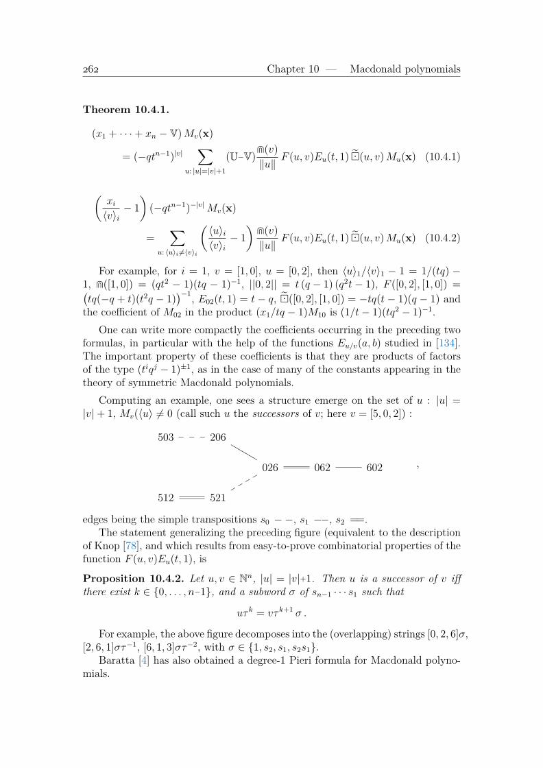
Chapter 10 — Macdonald polynomials
Theorem 10.4.1.
(x1 + · · ·+ xn − V)Mv(x)
= (−qtn−1)|v|∑
u: |u|=|v|+1
(U−V)e(v)
‖u‖F (u, v)Eu(t, 1) (u, v)Mu(x) (10.4.1)
(xi〈v〉i− 1
)(−qtn−1)−|v|Mv(x)
=∑
u: 〈u〉i 6=〈v〉i
(〈u〉i〈v〉i− 1
)e(v)
‖u‖F (u, v)Eu(t, 1) (u, v)Mu(x) (10.4.2)
For example, for i = 1, v = [1, 0], u = [0, 2], then 〈u〉1/〈v〉1 − 1 = 1/(tq) −1, e([1, 0]) = (qt2 − 1)(tq − 1)−1, ||0, 2|| = t (q − 1) (q2t− 1), F ([0, 2], [1, 0]) =(tq(−q + t)(t2q − 1)
)−1, E02(t, 1) = t− q, ([0, 2], [1, 0]) = −tq(t− 1)(q − 1) andthe coefficient of M02 in the product (x1/tq − 1)M10 is (1/t− 1)(tq2 − 1)−1.
One can write more compactly the coefficients occurring in the preceding twoformulas, in particular with the help of the functions Eu/v(a, b) studied in [134].The important property of these coefficients is that they are products of factorsof the type (tiqj − 1)±1, as in the case of many of the constants appearing in thetheory of symmetric Macdonald polynomials.
Computing an example, one sees a structure emerge on the set of u : |u| =|v|+ 1, Mv(〈u〉 6= 0 (call such u the successors of v; here v = [5, 0, 2]) :
503 ___ 206
LLLLLLL
026
r r r r062 602 ,
512 521
edges being the simple transpositions s0 −−, s1 −−, s2 ==.The statement generalizing the preceding figure (equivalent to the description
of Knop [78], and which results from easy-to-prove combinatorial properties of thefunction F (u, v)Eu(t, 1), is
Proposition 10.4.2. Let u, v ∈ Nn, |u| = |v|+1. Then u is a successor of v iffthere exist k ∈ 0, . . . , n−1, and a subword σ of sn−1 · · · s1 such that
uτ k = vτ k+1 σ .
For example, the above figure decomposes into the (overlapping) strings [0, 2, 6]σ,[2, 6, 1]στ−1, [6, 1, 3]στ−2, with σ ∈ 1, s2, s1, s2s1.
Baratta [4] has also obtained a degree-1 Pieri formula for Macdonald polyno-mials.

§ 10.5 — Transitions
10.5 TransitionsAs for Schubert polynomials, choosing an appropriate i for the product xiMv(x)provides a recursion on the Macdonald basis, that we shall still call a transition.
Proposition 10.5.1. Given u ∈ Nn, let k = max(u), i be the leftmost position ofk in u. Let v = [. . . , ui−1, k− 1, ui+1, . . .], and β be such that 〈v〉i = qk−1tβ. Then
Mu(x) = (xiq−k+1 − tβ)Mv(x) + tβ
∑w
Mv(〈w〉)‖w‖
(1− 〈w〉i〈v〉i
)Mw(x) , (10.5.1)
summed over the successors w of v such that 〈w〉i 6= 〈v〉i, and w 6= u. Moreover,for such w, one has w < u.
Proof. We have evaluated Mv(〈w〉) in Prop. 10.3.3. There remains only to checkthe statement about the order, that we skip. QED
Notice that the exponent β is equal to
n− 1−#(j : j > i, uj = k)−#(j : j < i, uj = k−1) . (10.5.2)
In other words, representing u by a diagram of boxes of coordinates (1, 0), . . . ,(1, u1−1), . . . , (n, 0), . . . , (n, un−1), then β is equal to the number of points (k, j), j >i and (k−1, j), j < i which are not occupied by a box.
One can iterate the transition formula. This gives a canonical decomposi-tion of any Macdonald polynomial into sums of products of “shifted monomials”∏
(xiq−a − tb), the specialization t = 0 of these monomials being of degree |v|.
For example, writing ij for a factor tiqj − 1, starting with u = [2, 0, 2], one hasv = [1, 0, 2], 〈v〉 = [tq, 1, t2q2] and the following sequence of transitions :
M202 =(x1q
−1 − t)M102 +
10
22M022 ,
M022 =(x2q
−1 − t)M012 + tq
10 · 10
11 · 21M121 +
10 · 31
21 · 21M112 ,
M121 =(x2q
−1 − t)M111 +
10
21M112 ,
M112 =(x3q
−1 − 1)M111 ,
leading to polynomials of degree 3 that one assumes to be known by induction onthe degree.
To reduce the size of the output, let us represent each factor xj/qi−1 − tβ bya black square in the Cartesian plane (row i, column j) ( β is determined by i, j,according to (10.5.2)). Then the final outcome of the transitions for M202 is
· · ·· ·
10 · 10
11 · 22+· · ·· ·
10 · 10
11 · 22+· · · · ·
10
11+· · · · ·
10
11+· · ·· ·
10
22+· · · · ·
with leading term· · · · ·
= (x1q−1 − t)(x1 − t)(x3q
−1 − t)(x3 − 1).

Chapter 10 — Macdonald polynomials
Haglund, Haiman, Loehr [59] give a combinatorial formula for the componentof degree |u| of Mu, which involves, in general, another enumeration than theone by transition. Still another decomposition is furnished, in the symmetric andnon-homogeneous case, by Okounkov [159, 160, 161].
10.6 Symmetric Macdonald polynomialsIn the space Vλ, which has basis Mv : v↓= λ, one can build another basis Mv,still starting with Mλ↑ = Mλ↑, but using the spectral vector [0, 1, . . . , tn−1] thistime.
In the case n = 2, we have already used di = Ti + 1 = (txi − xi+1)∂i, wichsends polynomials onto polynomials symmetrical in xi, xi+1. This shows thatMλ is symmetrical in every pair of consecutive variables, hence symmetrical inx. However, in the space Vλ, there is only one symmetrical polynomial (up to ascalar): being invariant under each di/(1+t) determines the expansion in the basisMv, once knowing one coefficient. This polynomial is the symmetrical Macdonaldpolynomial of index λ, its component of degree |λ| being the original Macdonaldpolynomial [?].
Thus Mλ = Mλ↑dω is symmetrical, and moreover every Mvdω is symmetricaland proportional to the symmetric Macdonald polynomial belonging to the spaceVλ. As a consequence, one can study the symmetric polynomial by just using dω.There are other methods, in particular some operators on symmetric functionswhich are described in the book of Macdonald.
As a side remark, let us determine the image of (x,y) under dω. From(10.3.2), one obtains that this polynomial Gn(x,y) is also symmetrical in y.Writing the recursion Gn → Gn+1, one realizes that Gn(x,y) is equal to theGaudin-Izergin-Korepin function :
R(x,y)R(x, ty)
∆(x)∆(y)det
(1
xi − yj)(xi − tyj)
).
The relevance of this last function to the theory of Macdonald polynomials hasbeen pointed out by Warnaar [192], as well as physicists [70, 109].

§ 10.7 — Macdonald polynomials versus Key polynomials
10.7 Macdonald polynomials versus Key poly-nomials
The generation of Macdonald polynomials involves operators of the type
Ti +t− 1
γ − 1= πi(t− 1)− si +
t− 1
γ − 1,
with some γ’s, which are rational functions in q, t, given by a spectral vector.The limits t = 0 or t = ∞ clearly must have special properties. To study
them, it is better to take the Hecke relation (Ti − t1)(Ti − t2) = 0 instead of(Ti − t)(Ti + 1) = 0, and transform spectral vectors by t → −t1/t2, withoutchanging the affine induction.
Let us still denote, in this section, by Mv the homogeneous Macdonald poly-nomials with parameters t1, t2, q. The operators to use in the recursion are now
Ti +t1 + t2γ − 1
= πi(t1 + t2)− t2si +t1 + t2γ − 1
.
The first specialisation that we shall consider is t1 = 0, t2 = −1. Let usdenote Mv the specialisation t1 = 0, t2 = −1 of the normalized polynomialMv/coeff(Mv, x
v).In that case, the constant γ = 〈v〉i+1〈v〉−1
i used in the recursion Mv → Mvsi ,when vi < vi+1, is of the type qvi+1−vi(−t1/t2)α, with α > 1, and tends towards 0.The operator Ti + (t1 + t2)(γ − 1)−1 tends towards −πi + si + 1, which sends 1 to1 and xi + 1 to xi + xi+1. Thus this last operator is a divided difference πxi+1,xi
for the reversed alphabet. Therefore,
Mvsi = Mv πxi+1,xi . (10.7.1)
Suppose that we know thatMv = Nv +q ?, with Nv = Kvω(xω), and ? ∈ C[q](xn).Then (10.7.1) shows that, modulo q, Mvsi is still a key polynomial for the reversedalphabet xωn.
Let v be antidominant. The affine operation does not imply t1, t2. The prede-cessor of Mv under the affine operation is Mu, with u = [vn− 1, v1, . . . , vn−1]. Onehas
Mu = Nu + q∑
cuwxw = xu +
∑xu′+ q
∑cuwx
w ,
sum over monomials xu′ such that u′1 < u1 (because, by induction, Nu is a keypolynomial) and monomials xw such that w1 ≤ u1, with coefficients which arepolynomials in q.
Therefore
Mv = qu1
(q−u1xv +
∑q−u
′1xu
′τ + q∑
cuwq−w1xwτ
),
and the term of degree 0 in q is the single monomial xv.In conclusion, one has the following specialization property due to B. Ion [66].

Chapter 10 — Macdonald polynomials
Theorem 10.7.1. Let v ∈ N. Then the normalized Macdonald polynomialMv/(coeff(Mv, xv)
specializes, for t1 = 0, t2 = −1, q = 0 into the key polynomial
Kvω(xωn)
for the reversed alphabet xωn = xn, . . . , x1.
One could hope that the specialization t1 = 1, t2 = 0 be treated exactly inthe same manner. Let us still denote Mv the specialization t1 = 1, t2 = 0 of thenormalized Macdonald polynomials. One computes
M012 = x012
iiiiiiiiiiiiiii
UUUUUUUUUUUUUUU
UUUUUUUUUUUUUUU
M102 = x102 + x111 + 1qx012 M021 = x021 + x111 + 1
qx012
M120 = x120 + 1qx111 + 1
qx021
TTTTTTTTTTTTTM201 = x120 + 1
qx111 + 1
qx102
jjjjjjjjjjjjj
jjjjjjjjjjjjj
M210 = x210 + 1q?
There is no way that one can obtain M021 from M012 using an operator involvingonly x2, x3 !
However, one can read the hexagon upwards. The space Mv : v ↑ can begenerated starting fromM210, the arrowsMv →Mvsi being invertible when t1, t2, qremain generic. Indeed, for any i, any γ 6= 0, 1, one has(
Ti+t1+t2γ−1
)(Ti+
t1+t2γ−1−1
)=
(t1+
t1+t2γ−1
)(t1+
t1+t2γ−1−1
)= −
(t1γ+t2)(t1+t2γ)
(γ − 1)2.
Taking into account that we use the normalized polynomialsMv/coeff(Mv, xv),
we have the recursion1
coeffMv
(t1γ + t2)(t1 + t2γ)
t2(γ − 1)2
(Ti +
t1 + t2γ − 1
)= cMvsi ,
when vi > vi+1, with γ = 〈v〉i+1〈v〉−1i = q−α
(−t2t1
)β, α, β > 0, and some constant
c 6= 0. The extra factor −1/t2 is due to the fact that xi+1Ti = −t2xi. The limitt1 = 1, t2 = 0 of (t1γ+t2)(t1+t2γ)
t2(γ−1)2is 1 when β > 1 and 1 − q−α when β = 1, while
Ti + (t1 + t2)(γ − 1)−1 specializes into πi − 1 = πi. Therefore, up to a possiblefactor 1− q−α, one has
Mvsi = (1− q−α) Mv πi .
Hence, if Mv = Kv+q−1(?), then Mvsi = Kvsi+q
−1(??), with ? and ?? polynomialsin q−1.

§ 10.7 — Macdonald polynomials versus Key polynomials
It remains to determine Mv for v dominant. If vn > 0, then Mv = MuΦ, withu = vτ−1 = [vn− 1, v1, . . . , vn−1]. However, Mu = xu +
∑cuwx
w, with w1 ≥ u1. Byinduction on the degree |u|, one can suppose that Mu = Ku modulo q−1. SinceKu = xu +
∑xw with w1 > u1, one has MuΦ = q−u1xv + q−u1−1(?) and therefore
Mv = xv + q−1(?) as needed.In the case where vn = 0, one has recourse to another ingredient. For any
u ∈ Nn−1, one has Mu0 = Mu + xnq−1(?). Assuming that for u = [v1, . . . , vn−1]
dominant, one has Mu = xu + q−1(?), this implies that Mu0 = xu + q−1(??).In final, one has the following specialization theorem due to B.Ion [66].
Theorem 10.7.2. Let v ∈ N. Then the limit t1 = 1, t2 = 0, q = ∞ of thenormalized Macdonald polynomialMv/coeff(Mv, x
v) is equal to the key polynomialKv.
In both limits (t1 = 1, t2 = 0) and (t1 = 0, t2 = −1), we have eliminated q bysending it to ∞ or 0. Sanderson [180] shows that the limit t = 0 of the usual nor-malized homogeneous nonsymmetric Macdonald polynomial is equal to an affineDemazure character (for us, on the reversed alphabet xω). It would be interestingto further develop the combinatorics of these affine Demazure characters. In fact,they are all the polynomials generated from the polynomial 1 using Φ and thedivided differences πxi+1,xi , no other ingredient is needed. Since πi acts on keypolynomials by sorting indices, one needs only to describe the polynomials Mv
(equal to q||v|| times the specialization t = 0 of the usual homogeneous Macdonaldpolynomial) for v antidominant. The polynomials for v dominant are symmetri-cal, since they are obtained using a maximal product of πxi+1,xi , and in fact areequal to the Hall-Littlewood polynomials1.
For example, using key polynomials in the reversed alphabet x3, x2, x1, onehas
M013 = K310 + qK220 + qK211 + q2K112
from which one obtains, by sorting indices,
M310 = K013 + qK022 + qK112 + q2K112 .
This last polynomial is explained by enumerating all tableaux of evaluation 1123 =122131 ([2, 1, 1] is the conjugate of [3, 1]) together with their charge :
q03
2
1 1
+ q1 2 3
1 1+ q1 2
1 1 3+ q2 3
1 1 2.
1 There are several species of Hall-Littlewood polynomials. The relevant one is here Q′µ =∑t qc(t)sλ(t), sum over all tableaux of evaluation µ, λ(t) being the shape of the tableau, but one
has to conjugate partitions.

Chapter 10 — Macdonald polynomials
Reading the conjugate shapes, one obtains
q0s31 + q1s22 + (q1 + q2)s211 ,
which coincides with M310. A refinement of charge is needed to explain M013.Notice that one can define nonsymmetric Hall-Littlewood polynomials Pv, v ∈
Nn [30], by starting with all dominant monomials and using the spectral vector[tn−1, . . . , 1] (with the Hecke relations (Ti − t)(Ti + 1) = 0).
For example one has P310 = x310 = K310, P130 = K13 − tK22, P103 = t2
t+1K22 −
tK112 +K103 − tt+1K13 + t2K211 − tK202, P013 = K013 − tK022 − tK112.
The last polynomial is, indeed, the Hall-Littlewood polynomial indexed bythe partition [3, 1], and is the specialization q = 0 of the symmetric Macdonaldpolynomial, but, except in the dominant or antidominant case, the polynomialsPv are not specializations of Macdonald polynomials, and are not related to theaffine Demazure characters.

Chapter 11Hall-Littlewood polynomials
Hall-Littlewood polynomials are specializations of Macdonald polynomials. How-ever we shall study them independently in this chapter. This study is part of ajoint work with Jennifer Morse.
11.1 From a quadratic form on the Hecke alge-bra to a quadratic form on polynomials
We have defined in (1.8.5) the quadratic form ( , )H on the Hecke algebraHn. Sincewe can use linear bases of Hn, as we have used ∂σ, πσ, πσ, to generate basesof Pol(xn), a natural problem is to find a quadratic form on Pol(xn) compatiblewith ( , )H. We propose a t1t2 deformation of the form ( , ) defined in 2.4.1.
LetΘ :=
∏1≤i<j≤n
1− xix−1j
1+t2xit−11 x−1
j
.
Let us use it to define a bilinear form ( , )t1t2 on Pol by
(f , g)t1t2 = CT(f g♣Θ
)= CT
(f g♣
∏1≤i<j≤n
(1−xixj
)∞∑k=0
(−t2t1
xixj
)k)(11.1.1)
where ♣ is the automorphism, already met, defined by xi → 1/xn+1−i for 1 ≤ i ≤n, and where CT (f Θ) means
CT (f Θ) := CTxn(CTxn−1 (. . . (CTx1 (f Θ)) . . .)
).
Lemma 11.1.1. For i ≤ n−1, the operator Ti is adjoint to Tn−i with respect to( , )t1t2.
Proof. Same proof as in the case of πi and ( , ) seen in 2.4.1. As usual, one isreduced to the case of two consecutive variables. QED
269
Chapter 11 — Hall-Littlewood polynomials
As in the case of the form ( , ), one has to determine the scalar product oftwo monomials. Since (xu, xv)t1t2 = (xu−vω, 1)t1t2 , the answer is provided by thefollowing lemma 1 for which we refer to [30, Lemma 4.2].
Introduce a partial order on elements of Zn by using right sums (this ordersgeneralizes the dominance order on partitions in Nn):
v ≥ u ⇔ vn ≥ un & vn−1+vn ≥ un−1+un & vn−2+vn−1+vn ≥ un−2+un−1+un & . . .
Lemma 11.1.2. For any u ∈ Zn, then (xu, 1)t1t2 6= 0 if and only if |u| = 0 andu ≥ [0, . . . 0].
Proposition 11.1.3. Let λ, µ ∈ Nn be dominant, σ, ζ be two permutations in Sn.If λ 6= µ, then (xλTσ , x
µTζ)t1t2 = 0.If λ = µ, and if σ, ζ are of minimum length in their coset modulo the stabilizer
of λ, then(xλTσ , x
λTζ)t1t2 6= 0 ⇔ σω = ω(λ)ζ , (11.1.2)where ω(λ) is the element of maximal length of the stabilizer of λ. In that case(xλTσ , x
λTζ)t1t2 = 1.
Proof. In the case µ, λ different, suppose that λ1 = µ1, . . . , λr = µr, λr+1 < µr+1.Since Ti is adjoint to Tn−i, the nullity of (xλTσ , x
λTζ)t1t2 results from the nullityof (xλHn , x
µ)t1t2 . Each monomial xu appearing in the expansion of some xλTσis such that u ≤ λω. However, (xu, xµ)t1t2 6= 0 requires that u ≥ µω, henceλω ≥ µω, which is a contradiction.
In the case λ = µ, the same reasoning shows that (xu, xλ)t1t2 6= 0 only in thecase u = λω. The space xλHn has basis Uv : v↓= λ, and xλω occurs only in theexpansion of Uλ↑. Since (xλω, xλ)t1t2 = 1, one concludes. QED
When λ is strict, its stabilizer is reduced to the identity, and in that case, forany two permutations,
(xλTσ , xλTζ)t1t2 6= 0 ⇔ σω = ζ . (11.1.3)
On the other hand, (Tσ, Tζ)H is different from 0 if and only if σ = ωζ. Thus in
that case we have a perfect correspondence between the quadratic form on Hn
and the quadratic form on xλHn. When λ is not strict, the dimension of the spacexλHn is less than n!. This explains why we have to use the stabilizer of λ.
11.2 Nonsymmetric Hall-Littlewood polynomi-als
We have shown in [30] how to use the two adjoint Yang-Baxter bases ∇ωσ, dσto generate noncommutative Hall-Littlewood polynomials Uv and Uv, v ∈ Nn. Letus recall the construction. Given v ∈ Zn, denote 〈v〉 its standardization.
1t1 = 1, t2 = −t for [30]. By homogeneity, one recovers the case of a general pair t1, t2.

§ 11.3 — Adjoint basis with respect to ( , )
When λ is dominant, then
Uλ = Uλ = xλ .
For v and i such that vi > vi+1, then
Uvsi = UvTi(〈v〉i − 〈v〉i+1
)& Uvsi = UvTi
(〈−v〉i − 〈−v〉i+1
)(11.2.1)
For example, for v = [2, 2, 0], one has 〈v〉 = [2, 3, 1], 〈−v〉 = [1, 2, 3]; forv = [2, 0, 2], one has 〈v〉 = [2, 1, 3], 〈−v〉 = [1, 3, 2] and for v = [0, 2, 2], one has〈v〉 = [1, 2, 3], 〈−v〉 = [3, 1, 2]. Accordingly
x220 = U220T2(2)−−→ U202
T1(1)−−→U022 ,
x220 = U220T2(−1)−−−→ U202
T1(−2)−−−→U022 .
The fact that ∇ωσ and dσ are adjoint bases with respect to ( , )H has itscounterpart at the level of polynomials.
Theorem 11.2.1. The two sets of polynomials Uv : v ∈ Nn and Uv : v ∈Nn are two adjoint bases of Pol with respect to the scalar product ( , )t1t2. Moreprecisely, they satisfy
(Uv , Uuω)t1t2 = δv,u .
Proof. If u ↓ or v ↓ are strict, then the statement results from (11.1.3). One hasjust to check that (xλTω, x
λ)t1t2 = (xλω, xλ)t1t2 = 1. In the non strict case, onehas to replace (11.1.3) by (11.1.2). QED
Notice that, we had met the pairing σ ↔ ωσ for bases of the Hecke algebra,while we have now the pairing v ↔ vω.
11.3 Adjoint basis with respect to ( , )
Using the quadratic form ( , ) instead of ( , )t1t2 , one obtains a basis, denoted Vv,v ∈ Nn, adjoint to Uv. The transition matrix Vv → Ku is the transpose of thetransition matrix Kv → Uu, and should be investigated.
For example, the rows of the following matrix describe the expansions of Vv,

Chapter 11 — Hall-Littlewood polynomials
v ∈ Nn, |v| = 3.
300 1 0 0 0 0 0 tt+1
0 0 0
210 0 1 0 0 0 0 0 0 0 0
201 0 0 1 0 0 0 0 tt+1
0 0
120 0 0 0 1 0 tt+1
t 0 0 0
111 0 0 0 0 1 t 0 t t (t+ 1) t3
102 0 0 0 0 0 1 0 0 0 0
030 0 0 0 0 0 0 1 0 0 0
021 0 0 0 0 0 0 0 1 0 0
012 0 0 0 0 0 0 0 0 1 t
003 0 0 0 0 0 0 0 0 0 1
Row 111 reads
V111 = K111 + tK201 + tK120 + t (t+ 1) K210 + t3K300 .
A bigger example
V421 = K421 + tK511 + tK430 + t(t+1)K520 + t2(t+1)K610 + t4K700 + t2K601
shows that the charge of tableaux of commutative evaluation 14223 explains theterms Kµ, µ dominant, the term t2K601 being apart.
11.4 Symmetric Hall-Littlewood polynomials fortypes A,B,C,D
For the remainder of this chapter, take t1 = 1, t2 = −t, and write ( , )t for thecorresponding specialization of ( , )t1t2 .
The polynomials Uλ↑ are symmetrical, being in the image of dω. More precisely,taking into account the stabilizer of λ, the recursive definition of Uλσ implies
Uλ↑ = b−1λ xλ
∏i<j≤n
(1− txjx−1i )πω , (11.4.1)
where bλ =∏
i
((1−t) · · · (1−tαi)
)= 1dω(λ), writing λ = 0α01α12α2 · · · in exponen-
tial form, ω(λ) being the permutation of maximal length in the stabilizer of λ (wehave taken λ ∈ Nn, with eventual terminal 0’s, contrary to the usual conventions).This equation is precisely the definition by Littlewood [144] of the Hall-Littlewoodfunction Pλ:
Uλ↑ = Pλ .
Identifying the pairs xjx−1i with the negative roots of the root system of type
A, one naturally extends the definition of Hall-Littlewood polynomials to all types.

§ 11.5 — Atoms
Let R♥ be the set of positive roots of the root system of type ♥ = A,B,C,D.Then for any ♥-dominant weight λ, one defines the Hall-Littlewood polynomialP♥λ by
P♥λ = b−1λ
∏α∈R♥
(1− te−α) π♥w0, (11.4.2)
where bλ is such that the coefficient of xλ be 1 in P♥λ .For example, for n = 3, one has
PBλ = b−1
λ xλ(
1−tx2
x1
)(1−
t
x1x2
)(1−tx3
x1
)(1−
t
x1x3
)(
1−tx3
x2
)(1−
t
x2x3
)(1−
t
x1
)(1−
t
x2
)(1−
t
x3
)πBw0
PCλ = b−1
λ xλ(
1−tx2
x1
)(1−
t
x1x2
)(1−tx3
x1
)(1−
t
x1x3
)(1−tx3
x2
)(
1−t
x2x3
)(1−
t
x12
)(1−
t
x22
)(1−
t
x32
)πCw0
PDλ = b−1
λ xλ(
1−tx2
x1
)(1−
t
x1x2
)(1−tx3
x1
)(1−
t
x1x3
)(
1−tx3
x2
)(1−
t
x2x3
)πDw0
.
Notice that∏
α∈R♥(1−te−α) π♥w0specializes, for t = 1, to the operator
∑w∈W w.
This leads to define, for λ dominant, a ♥-monomial function m♥λ to be the nor-malized image of xλ under
∑w∈W w.
11.5 AtomsInstead of using the full set of positive roots, let us delete the simple roots anduse the operator
f♥ =∏
α∈R\S
(1− te−α) π♥w0. (11.5.1)
For n = 3, these operators are
fB =
(1−tx3
x1
)(1−
t
x1x2
)(1−
t
x1x3
)(1−
t
x2x3
)(1−
t
x1
)(1−
t
x2
)πBw0
fC =
(1−tx3
x1
)(1−
t
x1x2
)(1−
t
x1x3
)(1−
t
x2x3
)(1−
t
x12
)(1−
t
x22
)πCw0

Chapter 11 — Hall-Littlewood polynomials
fD =
(1−tx3
x1
)(1−
t
x1x2
)(1−
t
x1x3
)πDw0
.
With these restricted sets of roots, one defines atoms A♥λ , λ dominant, to be
A♥λ = xλ f♥ . (11.5.2)
We shall show that the functions A♥λ and P♥λ are related by the Moebiusfunction of the dominance order on dominant weights, but we have first to say afew words about this order.
In type A, lower intervals for the dominant order can be defined by using theexpansion of Schur functions in terms of monomials. Indeed, for two partitions,ν ≤ λ if and only if xν occurs in the expansion of sλ.
One adopts the same definition in type B,C,D. Given two dominant weights,then ν ≤♥ λ if and only if xν occurs in the expansion of xλπ♥w0
.For example, for n = 3, and the weight λ = [3, 1, 1], the different sets ν ≤ λ
are:type A : [2, 2, 1], [3, 1, 1]
type B : [0, 0, 0], [1, 0, 0], [1, 1, 0], [1, 1, 1], [2, 0, 0], [2, 1, 0], [2, 1, 1],
[2, 2, 0], [2, 2, 1], [3, 0, 0], [3, 1, 0], [3, 1, 1]
type C : [1, 0, 0], [1, 1, 1], [2, 1, 0], [2, 2, 1], [3, 0, 0], [3, 1, 1]
type D : [1, 0, 0], [1, 1,−1], [1, 1, 1], [2, 1, 0], [2, 2, 1], [3, 0, 0], [3, 1, 1]
We have to adapt the definition of |λ| and n(λ) to take into account that intype D, for n odd, the last component of a dominant weight may be negative.Thus let ||λ|| :=
∑|λi|, n(λ) = 0λ1 + · · ·+ (n−2)λn−1 + (n−1)|λn|.
Then the expression of A♥λ in terms of P♥ν by a mere summation over the lowerinterval of λ, and conversely, the expression of P♥λ in terms of A♥ν is given by asummation involving the Moebius function of the interval.
Theorem 11.5.1. Let ♥ be A,B,C or D, and λ be a dominant weight for thistype. Then
A♥λ =∑ν≤♥λ
tk(||λ||−||ν||)+n(ν)−n(λ) P♥ν , (11.5.3)
P♥λ =∑ν≤♥λ
µ♥(λ, µ) tk(||λ||−||ν||)+n(ν)−n(λ) A♥ν , (11.5.4)
were µ♥( , ) is the Moebius function of the dominance order, with k = 0 in typeA, n in type B, n− 1/2 in type C, n−1 in type D.
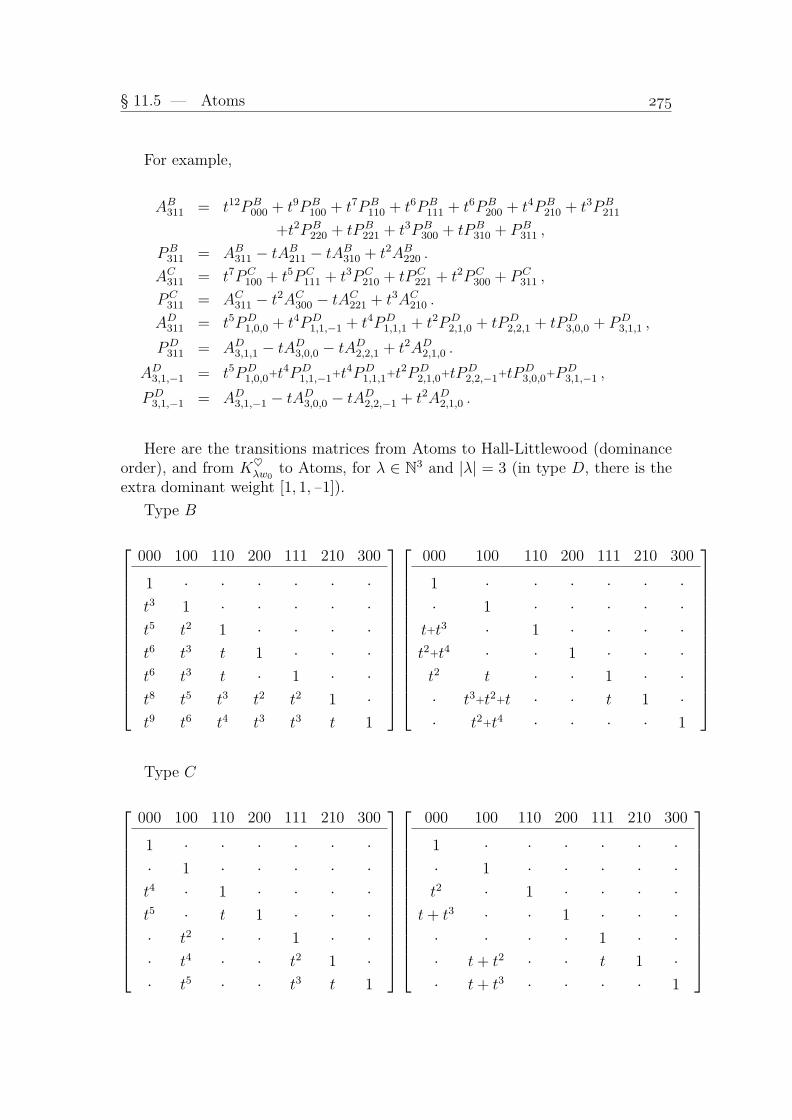
§ 11.5 — Atoms
For example,
AB311 = t12PB000 + t9PB
100 + t7PB110 + t6PB
111 + t6PB200 + t4PB
210 + t3PB211
+t2PB220 + tPB
221 + t3PB300 + tPB
310 + PB311 ,
PB311 = AB311 − tAB211 − tAB310 + t2AB220 .
AC311 = t7PC100 + t5PC
111 + t3PC210 + tPC
221 + t2PC300 + PC
311 ,
PC311 = AC311 − t2AC300 − tAC221 + t3AC210 .
AD311 = t5PD1,0,0 + t4PD
1,1,−1 + t4PD1,1,1 + t2PD
2,1,0 + tPD2,2,1 + tPD
3,0,0 + PD3,1,1 ,
PD311 = AD3,1,1 − tAD3,0,0 − tAD2,2,1 + t2AD2,1,0 .
AD3,1,−1 = t5PD1,0,0+t4PD
1,1,−1+t4PD1,1,1+t2PD
2,1,0+tPD2,2,−1+tPD
3,0,0+PD3,1,−1 ,
PD3,1,−1 = AD3,1,−1 − tAD3,0,0 − tAD2,2,−1 + t2AD2,1,0 .
Here are the transitions matrices from Atoms to Hall-Littlewood (dominanceorder), and from K♥λw0
to Atoms, for λ ∈ N3 and |λ| = 3 (in type D, there is theextra dominant weight [1, 1, −1]).
Type B
000 100 110 200 111 210 300
1 · · · · · ·t3 1 · · · · ·t5 t2 1 · · · ·t6 t3 t 1 · · ·t6 t3 t · 1 · ·t8 t5 t3 t2 t2 1 ·t9 t6 t4 t3 t3 t 1
000 100 110 200 111 210 300
1 · · · · · ·· 1 · · · · ·
t+t3 · 1 · · · ·t2+t4 · · 1 · · ·t2 t · · 1 · ·· t3+t2+t · · t 1 ·· t2+t4 · · · · 1
Type C
000 100 110 200 111 210 300
1 · · · · · ·· 1 · · · · ·t4 · 1 · · · ·t5 · t 1 · · ·· t2 · · 1 · ·· t4 · · t2 1 ·· t5 · · t3 t 1
000 100 110 200 111 210 300
1 · · · · · ·· 1 · · · · ·t2 · 1 · · · ·
t+ t3 · · 1 · · ·· · · · 1 · ·· t+ t2 · · t 1 ·· t+ t3 · · · · 1

Chapter 11 — Hall-Littlewood polynomials
Type D
000 100 110 200 111 111 210 300
1 · · · · · · ·· 1 · · · · · ·t3 · 1 · · · · ·t4 · t 1 · · · ·· t · · 1 · · ·· t · · · 1 · ·· t3 · · t2 t2 1 ·· t4 · · t3 t3 t 1
000 100 110 200 111 111 210 300
1 · · · · · · ·· 1 · · · · · ·
t+t2 · 1 · · · · ·t2 · · 1 · · · ·· · · · · 1 · ·· · · · 1 · · ·· t · · t t 1 ·· t2 · · · · · 1
The following property of the specialization in t = 1 of the functions A♥λ has
been obtained by Postnikov [168].
Corollary 11.5.2.A♥λ
∣∣∣t=1
=∑ν≤♥λ
m♥ν
For example, AD2,1,−1
∣∣t=1
= x0,0,0+x2,0,0+x0,2,0+x1,1,0+x1,0,−1+x1,−1,0+x−2,0,0+x0,0,−2 + x0,−2,0 + x−2,−1,−1 + x0,0,2 + x0,−1,−1 + x0,1,1 + x1,0,1 + x−1,0,−1 + x−1,−1,0 +x−1,−1,−2 + x−1,2,1 + x−1,1,2 + x−2,1,1 + x0,1,−1 + x0,−1,1 + x2,1,−1 + x1,2,−1 + x2,−1,1 +x1,−1,2 + x1,−2,1 + x−1,−2,−1 + x1,1,−2 + x−1,1,0 + x−1,0,1 has indeed no multiplicity.
11.6 Q′-Hall-Littlewood functionsBy definition the Q′-Hall-Littlewood functions are the symmetric functions suchthat
(Pλ, Q′µ) = δλ,µ .
We have defined a basis Vv which is adjoint to Uv. Since Pλ = Uλ↑, one has
(Pλ, Vµ) = δλ,µ = (Pλ, Vµπω) .
HenceQ′µ = Vµ πω . (11.6.1)
From the expansion of Vµ in the basis Kv, one obtains the expansion of Q′µ inthe basis of Schur functions, since Kvπω = 0 if v is not dominant, and Kλπω = sλif λ is a partition.
This expansion is positive, and coefficients have been interpreted in terms ofcharge of tableaux. Denote by Tabµ the set of tableaux of evaluation µ. Then onehas [119]:

§ 11.6 — Q′-Hall-Littlewood functions
Proposition 11.6.1. Let µ be a partition. For a tableau T , denotes λ(T ) itsshape, and c(T ) its charge. Then
Q′µ =∑
T∈Tabµtc(T )sλ(T ) . (11.6.2)
The set Tabµ has a structure of rank poset given by the cyclage [118, 116]. Ifν ≤ µ with respect to the dominance order, then Tabν is canonically isomorphicto a subposet of Tabµ. The complement in Tabµ of all the subposets isomorphicto Tabν : ν < µ is a poset called atom2 and denoted A(µ) [98].
Using the Möbius function (−1)〈µ,ν〉 of the lattice of partition to define functionsQ′′µ, one has [98]
Proposition 11.6.2. Let µ be a partition. Then
Q′′µ :=∑ν≤µ
(−1)〈µ,ν〉tn(ν)−n(µ) Q′ν =∑
T∈A(µ)
tc(T )sλ(T ) . (11.6.3)
For example, for µ = [3, 2, 1, 1], the atom is
A([3, 2, 1, 1]) =
432 21 1 1
32 21 1 1 4
32 2 41 1 1
2 2 41 1 1 3
and this gives
Q′′3211 = Q′3211 − tQ′322 − tQ′322 + 0Q′331 + t3Q′421 = s3211 + ts421 + ts331 + t2s43 .
In summary, one has
Proposition 11.6.3. With respect to ( , ), Q′λ is the basis adjoint to Pλ andQ′′λ is the basis adjoint to Aλ.
Both scalar products (sλ, Q′µ) and (sλ, Q
′′µ) are equal to sums
∑tc(T ) over sub-
sets of tableaux of shape λ, tableaux of weight µ in the first case, tableaux in A(µ)in the second case.
2In [98], one rather takes the image of A(µ) into the set of standard tableaux, i.e. tableauxwith weight [1, . . . , 1].

Chapter 11 — Hall-Littlewood polynomials
The following matrices record the scalar products (sλ, Q′′µ). Rows must be read
as the expansion of Schur functions in the basis Aλ, columns give the expansionof the functions Q′′µ in the Schur basis.
3 1 · ·21 · 1 t
111 · · 1
4 1 · · · ·31 · 1 · t t3
22 · · 1 · t2
211 · · · 1 t2 + t
1111 · · · · 1
5 1 · · · · · ·41 · 1 · t · t3 t6
32 · · 1 · t t2 t5 + t4
311 · · · 1 · t2 + t t5 + t4 + t3
221 · · · · 1 t t3 + t2 + t4
2111 · · · · · 1 t3 + t2 + t
11111 · · · · · · 1
6 51 42 411 33 321 3111 222 2211 21111 111111
1 · · · · · · · · · ·
· 1 · t · · t3 · · t6 t1·
· · 1 · · t t2 t2 · t5+t4 t9+t8+t7
· · · 1 · · t2+t · · t5+t4+t3 t9+t8+t7+t6
· · · · 1 · · · t2 t4 t8+t6
· · · · · 1 t t t t4+2 t3+t2 t8+2 t7+2 t6+2 t5+t4
· · · · · · 1 · · t3+t2+t t7+t6+2 t5+t4+t3
· · · · · · · 1 · t2 t6+t5+t3
· · · · · · · · 1 t2+t 2 t4+t5+t6+t3+t2
· · · · · · · · · 1 t4+t3+t2+t
· · · · · · · · · · 1

Chapter 12Kazhdan-Lusztig bases
We have already used the Hecke algebra Hn to generate bases of polynomials(Macdonald polynomials, Hall-Littlewood polynomials). Kazhdan and Lusztighave defined a linear basis Cw : w ∈ Sn with which we shall build still anotherlinear basis of Pol(xn) in this chapter.
12.1 Basis of the Hecke algebraWe take the Hecke algebra of type A with algebraic generators satisfying the Heckerelations (Ti− t1)(Ti− t2) = 0. It has a linear basis Tw : w ∈ Sn. Many familiesof interesting elements in the group algebra of Sn are globally invariant under theinversion of permutations. However Tw−1 6= (Tw)−1, when w is not the identity,the Hecke algebra has more subtle symmetry properties than the group algebra.
Kazhdan and Lusztig [72] defined a basis which is invariant under the involu-tion
ι : Tw → (Tw−1)−1 , t1 → −t2, t2 → −t1 ,
and has many interesting properties. In particular this basis gives informationabout singularities of Schubert varieties and of specializations of Schubert poly-nomials.
Requiring invariance under ι is not enough to characterize the basis. Forexample, 1, T1−t1 and 1, T1−t2 are two bases of H2 which could be candidateto replace the basis 1, s1 of C[S2].
One has to complete the condition of being invariant under ι by a conditionof “positivity“.
Definition 12.1.1. An element∑cwTw is t-positive if and only if the coefficients
cw belong to the linear span of the monomials tα1 tβ2 with α > β.
The following theorem is due to Kazhdan and Lusztig [72].
279

Chapter 12 — Kazhdan-Lusztig bases
Theorem 12.1.2. There exist a unique linear basis Cw of Hn, called Kazhdan-Lusztig basis, such that
Cw = Tw +∑v<w
P vw(t1, t2)Tv
is invariant under the involution ι, with t-positive coefficients P vw(t1, t2) (the sum-
mation is over the Ehresmann-Bruhat order).
The specializations P vw(−1, t2) are called Kazhdan-Lusztig polynomials.
Thus, with the positivity condition, we have discriminated between T1−t1 andT1−t2, and must have
Ci := Csi = Ti−t1 = Ti(−1) .
In length 2, one has, for i 6= j,
Csisj = CiCj = TiTj − t1Ti − t1Tj + t21 .
However,
C1C2C1 = T321 − t1T231 − t1T312 + (t21 − t1t2)T213 + t21T132 − (t31 − t21t2)T123
exhibits a violation t1t2T213. In fact, the absence of symmetry in T1, T2 is also agood reason to exclude C1C2C1 . This can be repaired by taking
C1
(C2 −
t1t2t1 − t2
)C1 =
∑w∈S3
(−t1)3−`(w)Tw ,
which satisfies all the requirements to be a Kazhdan-Lusztig element.However,
C1C2C1 = T321 − t1T231 − t1T312 + (t21 − t1t2)T213 + t21T132 − (t31 − t21t2)T123
exhibits a violation t1t2T213. In fact, the absence of symmetry in T1, T2 is also agood reason to exclude it. This can be repaired by taking
C1
(C2 −
t1t2t1 − t2
)C1 =
∑w∈S3
(−t1)3−`(w)Tw ,
which satisfies all the requirements to be a Kazhdan-Lusztig element.More generally, once known their existence, the strategy to build recursively
the Kazhdan-Lusztig elements is clear. Knowing Cw, given i such that `(wsi) >`(w), one computes f = CwCi. Enumerating permutations v < w by decreasinglength, one replaces, for each term of the type tj1t
j2Tv, f by f − tj1t
j2Cv, and iterate
till arriving to the identity permutation. The final value of f is equal to Cwsi . Insummary, there exists integers µ(v, w) such that
Cwsi = CwCi +∑
µ(v, w)(−t1t2)(`(w)−`(v)+1)/2Cv , (12.1.1)

§ 12.2 — Duality
sum over a certain subset1 of permutations smaller than w.For example, the above expression of C1C2C1 can be rewritten C321 = C231C1+
t1t2C1.Though the preceding algorithm is very simple to implement, it is unsatisfac-
tory because it does not shed much light over the Kazhdan-Lusztig elements andpolynomials.
Notice that all v appearing in (12.1.1) must be such that `(v) > `(vsi). Indeed,the image of this equation by right multiplication by Ci is
CwsiCi = (t2−t1)CwCi −∑
µ(v, w)(−t1t2)(`(w)−`(v)+1)/2CvCi ,
and the unicity of the basis implies that for each v appearing in the summationone has CvCi = (t2−t1)Cv.
For example, for w = [3, 4, 5, 1, 2], one has
C34512C2 = C35412 − t1t2C34152 − t1t2C34215 + t21t22C1,4,3,2,5 ,
and all permutations v appearing in the right hand side are such that v2 > v3.
12.2 DualityWe have introduced in (1.8.5) a quadratic form such that Tωσ is the basis adjointto Tσ : σ ∈ Sn. Thus, the coefficients P v
w(t1, t2) may be expressed as
P vw(t1, t2) =
(Cw , Tωv
)H.
Taking any total order compatible with the Bruhat order, one has the propertythat the transition matrix between Cw and Tw is unitriangular. It is naturalto invert it, here it is for n = 3 (read by rows):
123 132 213 312 231 321
123 1 0 0 0 0 0
132 t1 1 0 0 0 0
213 t1 0 1 0 0 0
312 t12 t1 t1 1 0 0
231 t12 t1 t1 0 1 0
321 t13 t1
2 t12 t1 t1 1
.
For this small example, the inverse matrix is obtained by just changing t1 into −t1.We refer to [65, Prop. 7.13] for the next proposition which describes the inverseof the matrix of Kazhdan-Lusztig polynomials for general n.
1 Kazhdan and Lusztig characterize this subset in terms of a graph which, even in type A,presents much mystery.

Chapter 12 — Kazhdan-Lusztig bases
Proposition 12.2.1. For any pair of permutations: ν, ζ such that ν ≤ ζ, one has
∑z: ν≤z≤ζ
(Cz , Tων
)H((Cωz , Tζ
)H)t1→−t1,t2→−t2= δν,ζ . (12.2.1)
Equation 12.2.1 can be rewritten, using the KL involution on the second scalarproduct, as ∑
z: ν≤z≤ζ
(Cz , Tων
)H ((Cωz , Tζ
)H)t1↔t2= δν,ζ . (12.2.2)
Define, for any ζ ∈ Sn, Cζ to be the image of Cζ under the exchange of t1 andt2. Then, since Tων is the basis adjoint to Tν, Eq. 12.2.2 translates into thefollowing duality property.
Proposition 12.2.2. The basis Cζ : w ∈ Sn is adjoint to the basis Cν, i.e.one has (
Cων , Cζ
)H= δν,ζ . (12.2.3)
Notice that (12.2.3) is a statement about products CνCζ−1 , while (12.2.2)involves sums of products of KL-polynomials. For example, one has C45123 =
C3C2C1C4C3C2, C34512 = C2C1C3C2C4C3, and(C45123 , C34512
)H= 0, because the
coefficient of T54321 in the expansion of (C3C2C1C4C3C2)(C3C4C2C3C1C2
)is null.
Relation 12.1.1 can be used to describe the regular representation of the Heckealgebra, as well as its irreducible representations [72]. The matrixMω representingTω, i.e. describing the multiplication by Tω in the KL-basis, has special propertieswhich should be investigated. Its entries are[
Mω]ζ,ν
=(CζTω , Cων
)H.
The last column of this matrix is the list of the coefficients of Cω in the productsCζTω. One has(
CζTω , C1...n
)H= (Cζ , Tω)H =
((Cζ , Tω
)H)t1↔−t2,
using the KL-involution for the last equality. The last expression shows that thecoefficient of Cω in the product CζTω is equal to the image under the exchanget1 ↔ −t2 of the coefficient of T1...n in Cζ . In other words, the last column of Mω
furnishes the Kazhdan-Lusztig polynomials in the identity. For example,
C3412T4321 = (t42 − t1t32)C4321 + . . .
C3412 = (t41 − t31t2)T1234 + . . .
The inverse of the matrix Mω are described by the following proposition.
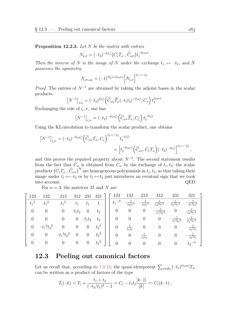
§ 12.3 — Peeling out canonical factors
Proposition 12.2.3. Let N be the matrix with entries
Nζ,ν = (−t2)−`(ζ)(CζTω , Cων
)t−`(ων)1 .
Then the inverse of N is the image of N under the exchange t1 ↔ −t2, and Npossesses the symmetry
Nων,ωζ = (−1)`(ζ)+`(ων)[Nζ,ν
]t1↔−t2.
Proof. The entries of N−1 are obtained by taking the adjoint bases in the scalarproducts: [
N−1]ν,ζ
= (−t2)`(ζ)(Cωζ Tω(−t1t2)−`(ω), Cν
)t`(ων)1 .
Exchanging the role of ζ, ν, one has[N−1
]ζ,ν
= (−t2)−`(ωζ)(CωνTω, Cζ
)t−`(ζ)1 .
Using the KL-involution to transform the scalar product, one obtains[N−1
]ζ,ν
= (−t2)−`(ωζ)(CωνTω, Cζ
)t1↔−t2t−`(ζ)1
=[t−`(ων)1
(Cων , CζTω
)(−t2)−`(ζ)
]t1↔−t2,
and this proves the required property about N−1. The second statement resultsfrom the fact that Cw is obtained from Cw by the exchange of t1, t2; the scalarproducts
(CζTω , Cων
)H are homogeneous polynomials in t1, t2, so that taking theirimage under t1↔−t2 or by t1↔ t2 just introduces an eventual sign that we tookinto account. QED
For n = 3, the matrices M and N are
123 132 213 312 231 321
t13 t1
2 t12 t1 t1 1
0 0 0 t1t2 0 t2
0 0 0 0 t1t2 t2
0 −t12t2
2 0 0 0 t22
0 0 −t12t2
2 0 0 t22
0 0 0 0 0 t23
123 132 213 312 231 321
t1−3 − 1
t2t13 − 1t2t13
1t22t13
1t22t13 − 1
t13t23
0 0 0 − 1t12t22 0 1
t23t12
0 0 0 0 − 1t12t22
1t23t12
0 1t1t2
0 0 0 − 1t23t1
0 0 1t1t2
0 0 − 1t23t1
0 0 0 0 0 t2−3
12.3 Peeling out canonical factorsLet us recall that, according to 1.9.12, the quasi-idempotent
∑w∈Sn
(−t1)`(ωw)Twcan be written as a product of factors of the type
Ti(−k) = Ti +t1 + t2
(−t2/t1)k − 1= Ci − t1t2
[k−1]
[k]=: Ci(k−1) ,

Chapter 12 — Kazhdan-Lusztig bases
with [k] = tk−11 − tk−2
1 t2 + · · · + (−t2)k−1 and [−k] = tk−12 − t1tk−1
2 + · · · + (−t1)k−1
for k > 0. The last expression is invariant under the KL involution, and therefore,for the permutation of maximal length of the symmetric group, one recognizes anelement already met several times,
Cω =∑w∈Sn
(−t1)`(ωw)Tw = ∇ω . (12.3.1)
In other words, all Kazhdan-Lusztig polynomials Pwω (−1, t2) are equal to 1. By
exchange of t1, t2, one has
Cω =∑w∈Sn
(−t2)`(ωw)Tw = dω . (12.3.2)
More generally, given a Young subgroup Sa×b×···, let ωa×b×··· be the permuta-tion of maximal length of this group. Then, by direct product, one has
Cωa×b×··· =∑
w∈Sa×b×···
(−t1)`(ωa×b×···w)Tw .
Under certain conditions on w, one can factor out from Cw some Cωa×b×··· .Let us just give a case that we shall need in the sequel. Given m, r : 1 ≤m < r ≤ n, denote by m,r,n = Cω1m,r−m,1n−r
, and by m,r,n the idempotentm,r,n[2]−1 · · · [r−m+1]−1.
Lemma 12.3.1. Let w ∈ Sn, m, r : 1 ≤ m < r ≤ n be such that wm > wm+1 >· · · > wr. Then there exists h ∈ Hn such that
Cw = hm,r,n . (12.3.3)
Proof. The preceding lemma has shown that Cw is invariant under right multipli-cation by the idempotent Ci/(t2−t1) for each i = m, . . . , r−1. Therefore, it mustbe invariant under the idempotent m,r,n.
Thus one can write
Cw =
(∑u
Quw(t1, t2)Tu
)m,r,n ,
sum over permutations u which are of minimum length in their cosetuS1m,r−m,1n−r . The coefficients Qu
w(t1, t2) must be polynomials in t1, t2, and notrational functions, and invariant under ι, otherwise the RHS would not be aKazhdan-Lusztig element. QED
The left factor h is not necessarily a Kazhdan-Lusztig element. For example,one has the factorizations
C321 =(T2T1 − t1T1 + t21
)C2 =
((T2 − t1)(T1 −
t21t1 − t2
)
)C2 ,
but the first left factor is not invariant under ι, being different from C312, and thesecond left factor does not have polynomial coefficients.

§ 12.4 — Non-singular permutations
Corollary 12.3.2. Let w ∈ Sn be such that there exists m < n : wn = n, andwm > wm+1 > · · · > wn. Let v = [w1, . . . , wm−1, wm+1, . . . , wn]. Then
Cw = Cv(Tn−1 . . . Tm − t1Tn−1 . . . Tm+1 + · · ·+ (−t1)n−m
)= CvTn−1(m−n) · · ·Tm(−1) . (12.3.4)
Proof. From the hypothesis on w, there exists h ∈ Hn such that Cv = hm,n−1,Cw = hm,n. The result follows fromm,n = m,n−1Tn−1(m−n) · · ·Tm(−1). QED
If the preceding corollary can be applied to w, or w−1, or ωwω, or ωw−1ω, saythat the permutation is peelable. allows to peel right or left factors from Cw. Inthe contrary case, and if w is not the identity, say that w is irreducible.
For example, let w = [4, 1, 7, 6, 2, 3, 5]. Then 1 is the first valley, one extractsT1(−1) from the right, and obtains w′ = [1, 4, 7, 6, 2, 3, 5]. Taking the inverse w” =[1, 5, 6, 2, 7, 4, 3], one sees that 7 is the last peak, and this allows the factorizationof T5(−1)T6(−2). One is left with [1, 4, 6, 5, 2, 3, 7]. Erasing the fixed points 1 and7, one sees that the ensuing permutation [4, 5, 1, 3, 2] cannot be reduced any more.The corollary has given
C4176235 = T5(−1)T6(−2)C1465237 T1(−1) = (T5T6−t1T6 + t21)C1465237(T1−t1) .
In fact, C4176235 factorizes totally, but this requires more work to be proved !
C4176235 = T5(−1)T6(2)(T3(−1)T2(−1)T5(−1)T4(−2)T3(−2)T5(−1)T4(−1)
)T1(−1) .
Let us call totally reducible a permutation such that there exists a chain ofreductions leading to the identity permutation.
12.4 Non-singular permutationsLet us call non-singular2 a permutation w such that
Cw =∑v≤w
(−t1)`(w)−`(v)Tv ,
i.e. such that all P vw(−1, t2), v ≤ w, are equal to 1.
Lakshmibai and Sandhya [90] have proved that a Schubert variety w is non-singular if and only if the indexing permutation avoids the patterns 3412 and 4231.Notice that in that case wω avoids 2143 and 1324, the first condition being thatwω be vexillary.
The following proposition [100] shows that the two notions, being non-singular,or being totally reducible, coincide.
2They are the permutations such that the corresponding Schubert varieties are non-singular.The relations between Kazhdan-Lusztig polynomials and Schubert varieties are explained in [73].

Chapter 12 — Kazhdan-Lusztig bases
Proposition 12.4.1. A permutation w is such that all P vw(−1, t2) are equal to 1
when v ≤ w iff it is totally reducible.
Proof. With the hypotheses of the last corollary, the set P uw(−1, t2), u ∈ Sn
coincides with the set P uv (−1, t2), u ∈ Sn. Therefore, if v is non-singular, then
w is so. The same reasoning is valid when the reduction applies to w−1, or ωwω,or ωw−1ω, instead of w.
Conversely, let w be irreducible and such that n is not a fixed point. If wavoids the pattern 3412, then one checks that w contains a subword of the type[. . . n . . . b . . . c . . . a], with a = wn, a < b < c. If w avoids the pattern 4231,then one checks that w contains a subword of the type [. . . c . . . n . . . a . . . b], withb = wn, a < b < c. QED
Thus, non-singularity can be controlled by looking for patterns 3412 and 4231,or testing recursively a condition on n and 1 inside w.
In the non-singular case, the preceding proposition gives a factorization [100]of Cw, and by specialization, of the Poincaré polynomial of the interval [1, w].
For example, w = [4, 1, 6, 5, 3, 2] is non-singular, Cw factorizes as
C416532 =
((T2(−1)T3(−2)
(T2(−1)T1(−1)
))T4(−2)T3(−1)
)T5(−3)T4(−2)T3(−1) .
Sending Ti → t2 transforms Ti(−k) into −[k+1]/[k]. Therefore the image of Cw =∑v≤w(−t1)`(w)−`(v)Tv, using the preceding factorisation, is equal to
−((
[2][3]
[2]
([2]2)) [3]
[2][2]
)[4]
[3]
[3]
[2][2] = −[2]2[3]2[4] .
Notice that we thus recover the fact that Cω factorizes into simple factors1.9.10:
C54321 = C1(0)C2(1)C1(0)C3(2)C2(1)C1(0)C4(3)C3(2)C2(1)C1(0) .
The factorization of the Poincaré polynomial in the non-singular case is dueto Carrell and Peterson [18]. The specialisation Ti = t2 of Cw has a geometricalinterpretation in terms of some sophisticated cohomology theories [73]. Noticethat, from a combinatorial point of view, using Kazhdan-Lusztig elements insteadof intervals with respect to the Ehresman-Bruhat order regularizes the special-ization. For example, the Poincaré polynomial for w = [3, 4, 1, 2] is equal to(t2 − t1)(t2
3 − 3t22t1 + 2t2t1
2 − t13), while C3412 specializes to (t2 − t1)4.

§ 12.5 — Kazhdan-Lusztig polynomial bases
12.5 Kazhdan-Lusztig polynomial basesWe have used the pair ∇ωσ, dσ of adjoint bases of Hn to generate a pairUv, Uvω of adjoint bases of Pol(xn). We shall see that the same constructionworks when starting from the pair of Kazhdan-Lusztig elements Cωσ, Cσ.Take t1 = 1, t2 = −t in this section.
As in the case of nonsymmetric Hall-Littlewood polynomials, some care isneeded when indices have equal components. Standardization provides the linkbetween elements of Nn and permutations. We have already used v → 〈v〉 thestandardization3 , reading from left to right, by increasing values. We need asecond one, the standardization by decreasing values, reading from right to left,that we denote 〈〈v〉〉. For example,
v = 2 0 3 2 0 2 3 0
2 15 4 3
8 7 6
〈〈v〉〉 = 5 8 2 4 7 3 1 6
Then, for any v ∈ Nn, with λ = v↓, one defines
Cxv =
xλ
bλC〈〈v〉〉 , (12.5.1)
and
Cxv =xλ
bλC〈−v〉 , (12.5.2)
where the constant bλ has been defined in (??).For example, for v = [2, 2, 0], [2, 0, 2], [0, 2, 2], one has 〈〈v〉〉 = [2, 1, 3], [2, 3, 1],
[3, 2, 1], and 〈−v〉 = [1, 2, 3], [1, 3, 2], [3, 1, 2]. Therefore
Cx220 =
x220
1+tC213 = x220 , Cx
202 =x220
1+tC231 , Cx
022 =x220
1+tC321 ,
Cx220 = x220 , Cx202 = x220 C132 , Cx022 = x220 C312 .
Using the explicit values of the Kazhdan-Lusztig elements, one finds
Cx220 =
x220
1+tT1(1) = x220 = U220 , C
x202 =
x220
1+tT1(1)T2(1) = U202 +
t
1+tU220 ,
Cx022 =
x220
1+tT1(1)T2(2)T1(1) = U022 ,
3We also standardize −v, that is, we standardize v from left to right by decreasing values.

Chapter 12 — Kazhdan-Lusztig bases
Cx220 = x220 = U220 , Cx202 = x220T2(−1) = U202 ,
Cx022 = x220T2(−1)(T1−1) = U022 −t
1+tU202 .
In the case where v = λ ↑ is antidominant, then Cxv = xλb−1
λ Cω = xλb−1λ dω,
and therefore is equal to the Hall-Littlewood polynomial Pλ(x1, . . . , xn). When λis strict (i.e. all parts are different), then
Cxv = xλ Cω = xλ∇ω = xλ ∂ω∏i<j
(xj−txi) = sλ−ρ(xn)∏i<j
(xj−txi) .
The same proof as for the bases Uv, Uvω (Theorem ??) gives the followingduality between Cxv , Cx
vω:
Theorem 12.5.1. The two sets of polynomials Cxv : v ∈ Nn and Cxv : v ∈ Nn
are two adjoint bases of Pol with respect to the scalar product ( , )t. More precisely,they satisfy
(Cxv , Cxuω)t = δv,u .
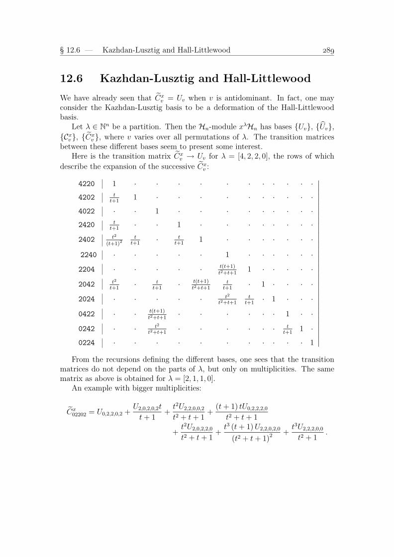
§ 12.6 — Kazhdan-Lusztig and Hall-Littlewood
12.6 Kazhdan-Lusztig and Hall-LittlewoodWe have already seen that Cx
v = Uv when v is antidominant. In fact, one mayconsider the Kazhdan-Lusztig basis to be a deformation of the Hall-Littlewoodbasis.
Let λ ∈ Nn be a partition. Then the Hn-module xλHn has bases Uv, Uv,Cxv , Cx
v , where v varies over all permutations of λ. The transition matricesbetween these different bases seem to present some interest.
Here is the transition matrix Cxv → Uv for λ = [4, 2, 2, 0], the rows of which
describe the expansion of the successive Cxv :
4220 1 · · · · · · · · · · ·
4202 tt+1
1 · · · · · · · · · ·
4022 · · 1 · · · · · · · · ·
2420 tt+1
· · 1 · · · · · · · ·
2402 t2
(t+1)2tt+1
· tt+1
1 · · · · · · ·
2240 · · · · · 1 · · · · · ·
2204 · · · · · t(t+1)t2+t+1
1 · · · · ·
2042 t2
t+1· t
t+1· t(t+1)
t2+t+1tt+1
· 1 · · · ·
2024 · · · · · t2
t2+t+1tt+1
· 1 · · ·
0422 · · t(t+1)t2+t+1
· · · · · · 1 · ·
0242 · · t2
t2+t+1· · · · · · t
t+11 ·
0224 · · · · · · · · · · · 1
∣∣∣∣∣∣∣∣∣∣∣∣∣∣∣∣∣∣∣∣∣∣∣∣∣∣∣∣∣∣∣∣∣∣∣From the recursions defining the different bases, one sees that the transition
matrices do not depend on the parts of λ, but only on multiplicities. The samematrix as above is obtained for λ = [2, 1, 1, 0].
An example with bigger multiplicities:
Cx02202 = U0,2,2,0,2 +
U2,0,2,0,2t
t+ 1+t2U2,2,0,0,2
t2 + t+ 1+
(t+ 1) tU0,2,2,2,0
t2 + t+ 1
+t2U2,0,2,2,0
t2 + t+ 1+t3 (t+ 1)U2,2,0,2,0
(t2 + t+ 1)2 +t3U2,2,2,0,0
t2 + 1.

Chapter 12 — Kazhdan-Lusztig bases
12.7 Using key polynomialsWe have seen that„ then Cw, for a nonsingular permutation w, is a sum over aninterval for the Ehresmann-Bruhat order. On the other hand, a key polynomialKv is also a sum of polynomials Ku over an interval for the same order. It is thusnatural to try to relate Kazhdan-Lusztig elements to key polynomials.
Let, for this section only, ρ = [1, . . . , n], and let Vρ be the linear span ofmonomials of exponents w ∈ Sn. Notice that xρTw ∩ Vρ = (−t2)`(w)xw Hence onehas
xρCw ∩ Vρ =∑v
(−t1)`(w)−`(v)P vw(t1, t2)(−t2)`(v)xv .
Define a linear morphism ϕ from Vρ to Pol(xn) by
ϕ(xv) = (−t2)`(v)xvω if v is a permutation , ϕ(xv) = 0 otherwise , (12.7.1)
with ϕ(t1) = −1, ϕ(t2) = t2. The preceding equation reads now
ϕ(xρCw) =∑v≤w
P vw(−1, t2)xvω . (12.7.2)
In particular, when w is non-singular, the image of the Kazhdan-Lusztig elementreduces to a single key polynomial:
ϕ(xρCw) =∑v≥wω
xv = Kwω ∩ Vρ (12.7.3)
For n = 4 there are only two singular permutations, which satisfy
C3412 = C2C3C1C2 , ϕ(x1234C3412) ≡ K2143 + t2K4231
C4231 = C3C2C1(1)C2C3 , ϕ(x1234C4231) ≡ K1324 + t2K3412 .
For n = 5, there are 32 singular permutations. Taking into account sym-metries, eliminating those permutations coming from [3, 4, 1, 2] or [4, 2, 3, 1], oneis left with only 8 permutations to study. We give a factorisation of Cw, writ-ing C+
i , C++i instead of Ci(1), Ci(2). Only C45312 does not factorize into simple
elements Ci(k). It can however be written
C45312 = C2C+3 C2
(C+
4 C+1 −
t31t32
(t2 − t1)2(t22 − t1t2 + t21)
)C2C
+3 C2 .
C45123 C3C2C1C4C3C2 K32154+t2K52341+t2K53142+t2K35241−t2K53241
C53412 C4C3C+2 C3C4C
+1 C2C3 K21435+t2K41523+t2K42315+t2K24513−t2K42513
C52341 C4C3C2C+1 C2C3C4 K14325+t2K45123+t2K34512+t22K45312
C45132 C3C4C+2 C
+3 C4C1C2 K23154 + t2K25341
C35142 C2C1C4C+3 C4C2 K24153 + t2K45231
C52431 C1C2C+3 C
++4 C2C
+3 C2C1 K13425 + t2K34512
C54231 C4C+3 C4C
+2 C3C
++1 C+
2 C3C4 K13245 + t2K34125
C45312 see above K21354 + t22K52341

§ 12.7 — Using key polynomials
From the table, by summation of the coefficients in the last column, one obtainsthe Kazhdan-Lusztig polynomials P 12345
w (−1, t2) :
P 1234545123 = P 12345
53412 = 1 + 2t2, P1234552341 = 1 + 2t2 + t22 ,
P 1234545132 = P 12345
35142 = P 1234552431 = P 12345
54231 = 1 + t2, P1234545312 = 1 + t22 .
The permutation [4, 5, 3, 1, 2] belongs to the family [n−1, n, n−2, . . . , 3, 1, 2]which give rise to the Kazhdan-Lusztig polynomials equal to 1 + tn−1
2 . These per-mutations are used by Polo [166] to build arbitrary Kazhdan-Lusztig polynomials.

Chapter 12 — Kazhdan-Lusztig bases
12.8 Parabolic Kazhdan-Lusztig polynomialsTaking the action of Kazhdan-Lusztig elements on a weight space Vλ, when λ hasrepeated parts, produce polynomials with coefficients which, in general, are linearcombinations of Kazhdan-Lusztig polynomials (see Deodhar [29]).
Let λ ∈ Nnbe a partition, v = λ ↑. Since (xixi+1)kCi = 0, then xvCσ = 0 ifthere exists i : vi = vi+1 and `(siσ) < `(σ). To avoid this nullity, given v, one hasto take any σ such that for any i : vi = vi+1, then σ contains the subword i, i+1.
One hasx12C1 = x12(T21 − t1T12) = −t2x21 − t1x12 .
To identify the action of C1 on x12 to the expression of C1 in the Tσ basis, one hasto normalize monomials by length4:
−t2x21 − t1x12 → −t2((−t2)−1x21
)− t1
((−t2)−0x12
).
More generally, given a partition λ, and an element in xvHn with v = λ ↑, onedefines ψλ to be the morphism∑
u:u↑=v
cuxu +
∑w:w↑6=v
cwxw →
∑cu
∣∣∣t1=1
(−t2)−`(u)xu .
One checks that for any σ ∈ Sn one has
ψλ (xvTσ) = xvσ , (12.8.1)
so that the action of the Hecke algebra on xv projects on the usual action of thesymmetric group.
Given a partition λ ∈ Nn, v = λ↑ and σ ∈ Sn such that xvCσ 6= 0, let w = vσ.Then
ψλ (xvCσ) = xw +∑u
(−1)`(w)−`(u)P uλ,σ(t2)xu
and the polynomials P uλ,σ(t2)xu are called parabolic Kazhdan-Lusztig polynomi-
als. The next proposition relates these polynomials to the usual Kazhdan-Lusztigpolynomials.
Given a composition α = [α1, . . . , αk], let β = 0α11α2 . . . (k−1)αk . The projec-tion of Sn onto Sα\Sn can be identified with the morphism
Sn 3 σpβ−−→βσ1 . . . βσn
from the symmetric group to words which are permuted of β.
4the length of an exponent u is defined to be the number of pairs such that ui > uj ,i < j, byextension of the case of a permutation.

§ 12.8 — Parabolic Kazhdan-Lusztig polynomials
Proposition 12.8.1. Given a partition λ ∈ Nn, v = λ ↑ and σ ∈ Sn such thatxvCσ 6= 0, let w = vσ. Then
P uλ,σ(t2) =
∑ν∈Sn: pv(ν)=u
(−1)`(σ)−`(ν)P νσ (−1, t2) . (12.8.2)
Proof. The statement is a direct consequence of (12.8.1). QEDFor example, let σ = [3, 4, 1, 2], v = [0, 0, 1, 1]. The correspondence between
xvC3412 = x1100 − x1010 + t2x0101 − t2x0011 and the expansion of C3412 in the Tw
basis is shown in the following enumeration (writing ν instead of Tν):
2143−1243 −2143
(1−t2)1234
−t2x0011+
−24132314 1423
(t2−1)1234
t2x0101
+
1432
−1342
0x0110+
3214
−3124
0x1010+
−3142
−x1010+
3412
x1100

Chapter 12 — Kazhdan-Lusztig bases
12.9 Graßmannian caseThe Kazhdan-Lusztig polynomials corresponding to Schubert subvarieties of Graß-mannians have been described in terms of increasing labelling of trees [120, 100].The relevant permutations are the coGraßmannian permutations, i.e. w ∈ Sn
issuch that there exists r : w1 > · · · > wr; wr+1 > · · · > wn.Let G(r, n) be the module Cr...1n...r+1Hn. It has a linear basis Cw, where the
w are coGraßmannian with a rise in r. Recall that, as an operator on polynomials,
Cr...1n...r+1 = ∂r...1n...r+1∆t2t1(x1, . . . , xr)∆t2t1(xr+1, . . . , xn)
where ∆t2t1(x1, . . . , xr) =∏
1≤i<j≤r(t2xi + t1xj).In particular, putting ρr,n−r = [r−1, . . . , 1, 0, n−r, . . . , 1, 0], one has
xρr,n−rCr...1n...r+1 = ∆t2t1(x1, . . . , xr)∆t2t1(xr+1, . . . , xn) .
The space ∆t2t1(x1, . . . , xr)∆t2t1(xr+1, . . . , x2r)H2r is in fact a representation
of the Temperley-Lieb algebra5, and together with its Kazhdan-Lusztig basis, hasbeen the object of numerous articles in the physics literature [43, 56, 70]. It hasalso a basis of Macdonald polynomials degenerated in q = −(t2/t1)3. The relationsbetween the Kazhdan-Lusztig basis and the Macdonald basis are described in [57].
Instead of computing in the space Cr...1n...r+1Hn, let us show that one obtainsmore simply the same Kazhdan-Lusztig polnomials using the dual basis Cv : v↓=1r0n−r. The elementary elements that one has to use are Ci = Ci(0) = Ti − t2,and their shifted versions:
C+i = Ci(1) = Ti +
t1 + t2(−t1/t2)2 − 1
= Ci −t1t2[2]
C++i = Ci(2) = Ti +
t1 + t2(−t1/t2)3 − 1
= Ci −t1t2[2]
[3]. . . . . .
Ci(k) = Ti +t1 + t2
(−t1/t2)k+1 − 1= Ci −
t1t2[k]
[k+1]
The description of the dual basis is made easier by interpreting the indices v asdescribing the border of the diagram of a partition. The correspondence betweenGraßmannian permutations w (with descent in r), v : v ↓= 1r0n−r and partitionsλ is
w ↔ v = [0w1−1, 1, 0w2−w1−1, 1, . . . , 0n−wr ]↔ λ = [wr−r, . . . , w1 − 1] .
Given a partition λ ∈ Nr, label recursively the boxes of the diagram of λ (usingmatrix conventions) as follows. Corners have label ` = 0. Erase them. The newcorners have labels ` = 1. &c. Iterate till exhausting all boxes.
00
0,
1 01 00
,2 1 0
1 00
,3 2 1 01 00
.
5 quotient of Hn by the relations Ti(1)Ti±1(2)Ti(1) = 0.
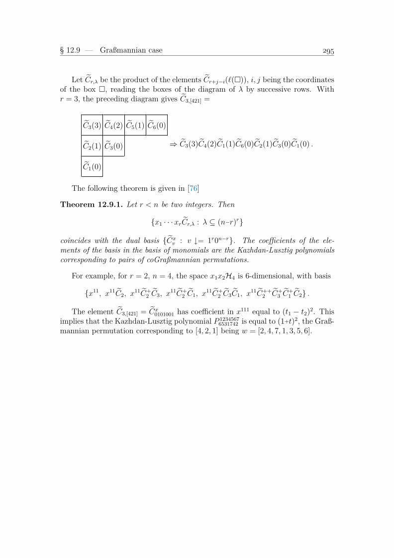
§ 12.9 — Graßmannian case
Let Cr,λ be the product of the elements Cr+j−i(`()), i, j being the coordinatesof the box , reading the boxes of the diagram of λ by successive rows. Withr = 3, the preceding diagram gives C3,[421] =
C3(3) C4(2) C5(1) C6(0)
C2(1) C3(0)
C1(0)
⇒ C3(3)C4(2)C1(1)C6(0)C2(1)C3(0)C1(0) .
The following theorem is given in [76]
Theorem 12.9.1. Let r < n be two integers. Then
x1 · · ·xrCr,λ : λ ⊆ (n−r)r
coincides with the dual basis Cxv : v ↓= 1r0n−r. The coefficients of the ele-
ments of the basis in the basis of monomials are the Kazhdan-Lusztig polynomialscorresponding to pairs of coGraßmannian permutations.
For example, for r = 2, n = 4, the space x1x2H4 is 6-dimensional, with basis
x11, x11C2, x11C+
2 C3, x11C+
2 C1, x11C+
2 C3C1, x11C++
2 C+3 C
+1 C2 .
The element C3,[421] = Cx0101001 has coefficient in x111 equal to (t1 − t2)2. This
implies that the Kazhdan-Lusztig polynomial P 12345676531742 is equal to (1+t)2, the Graß-
mannian permutation corresponding to [4, 2, 1] being w = [2, 4, 7, 1, 3, 5, 6].

Chapter 12 — Kazhdan-Lusztig bases
12.10 Dual basis and key polynomialsIn a preceding section, we have used that x1...nTw ∩ V1...n = (−t2)`(w)xw to relatethe Kazhdan-Lusztig basis to key polynomials.
On the other hand, the space x1 · · ·xrHn has linear basis the monomials withexponent v : v ↓= 1r0n−r, and thus has linear basis Kv as well as Kv = xv.In that case we can directly use the key polynomials without having to pass to aquotient space.
Under the specialization t1 to 1 and t2 to 0, the action of C1 becomes: x10C1 =t1(x1+x2) is sent to x1+x2, x01C1 = −t2(x1+x2) is sent to 0, and xiiC1 = (t1−t2)xii
is sent to xii. In other words, C1 acts like π1. Thus the dual Kazhdan-Lusztigbasis in the weight space V1r0n−r may be considered as a deformation of the basisof key polynomials.
For example, for r = 2, n = 5, the Kazhdan-Lusztig basis is indexed bypartitions contained in [3, 3] and has the following expansion in terms of the keypolynomials K11, K101, K1001, K10001, K011, K0101, K0011, K01001, K00101, K00011 :
[ ] 1 · · · · · · · · ·[1] · t1 · · · · · · · ·[2] · · t1
2 · · · · · · ·[3] · · · t1
3 · · · · · ·[1, 1] · · · · t1
2 · · · · ·[2, 1] −t12t2 · · · · t1
3 · · · ·[2, 2] · · · · · · t1
4 · · ·[3, 1] −t13t2 · · · · · · t1
4 · ·[3, 2] · · · · −t2 t14 · · · t1
5 ·[3, 3] · · · · · · · · · t1
6
Row [3,2], for example, has to be read C2,[32] = t51K00101 − t2t41K011.The Kazhdan-Lusztig polynomials P v
w(−1, t2) themselves are equal to the imageunder t1 → 1, t2 → −t2 of the coefficients in the basis Kv. For example, theexpansion
C3,[321] = t61K010101 − t2t51K0111 − t2t51K110001 +−t22t41K1101
furnishes the Kazhdan-Lusztig polynomials 1, 1 + t2, 1 + 2t2 + t22, the expansionof C3,[321] = Cx
010101 in the basis of monomials xv = Kv beingt1
4 (t1−t2)2 x111000 + t14 (t1−t2)2 x110100 + t1
5 (t1−t2)x011100 + t15 (t1−t2)x101100 +
t15 (t1−t2)x110010+t1
6x101010+t16x011010+t1
5 (t1−t2)x110001+t16x101001+t1
6x011001+t1
6x100110 + t16x010110 + t1
6x010101 + t16x100101.
The rule to read Kazhdan-Lusztig polynomials from a partition is given in[120, 100].

Chapter 13Complements
297

Chapter 13 — Complements
13.1 The symmetric group
13.1.1 PermutohedronGiven v ∈ Nn, one generates a directed graph I(v) by iterating sorting operationsu → usi if ui if vi > vi+1. This graph is in fact a rank lattice, with extremalelements v and v↑. The rank `(u) is the number of inversions (as for permutations,an inversion is a subword ji with j > i).
The set I(v) can be generated recursively by using a restricted shuffles definedas follows. For v ∈ Nn, k ∈ N, let i be such that vi · · · vn be the maximal leftfactor of v such that vj > k, j = i, . . . , n. Then
vsk = [v1, . . . , vi−1, k, vi, . . . , vn], [v1, . . . , vi, k, vi+1, . . . , vn], . . . , [v1, . . . , vn, k] .
It is clear thatI(v) = v1s v2s · · · s vn .
When v = [n, . . . , 1], the poset I(v) is called the (right) permutohedron, andthe underlying order on the symmetric group is called, unfortunately [11], the(right) weak order.
Another approach to intervals for the weak order is to replace sets of elementsof Sn by sums in the group algebra Z[Sn] or in the algebra Z[∂1, . . . , ∂n−1].
Let n =∑
σ∈Sn∂σ. We have already used that
∑σ∈Sn
σ =
∑σ∈Sn−1
σ
(1 + sn−1 + sn−1sn−2 + · · ·+ sn−1 · · · s1) (13.1.1)
= (1 + sn−1 + sn−2sn−1 + · · ·+ s1 · · · sn−1)∑
σ∈Sn−1
σ (13.1.2)
Correspondingly, one has
n = n−1 (1 + ∂n−1 + ∂n−1∂n−2 + · · ·+ ∂n−1 · · · ∂1) (13.1.3)= (1 + ∂n−1 + ∂n−2sn−1 + · · ·+ ∂1 · · · ∂n−1)n−1 . (13.1.4)
Factorizing further 13.1.1 requires using the Yang-Baxter relations ??. This isin fact easier in Z[∂1, . . . , ∂n−1]. Indeed
1 + ∂n−1 + ∂n−1∂n−2 + · · ·+ ∂n−1 · · · ∂1
= (1 + ∂n−1)(1 + ∂n−1∂n−2) · · · (1 + ∂n−1∂n−2 · · · ∂1)
because all products (∂n−1 · · · ∂i)(∂n−1 · · · ∂j) vanish. Therefore, one has
n = n−1 (1 + ∂n−1)(1 + ∂n−1∂n−2) · · · (1 + ∂n−1∂n−2 · · · ∂1) (13.1.5)= (1 + ∂1 · · · ∂n−1) · · · (1 + ∂n−2∂n−1)(1 + ∂n−1)n−1 . (13.1.6)

§ 13.1 — The symmetric group
The inverse of 1+∂n−1 · · · ∂i being 1−∂n−1 · · · ∂i, the element n has an inverse Ωn
which is equal to
Ωn = (1− ∂n−1∂n−2 · · · ∂1) · · · (1− ∂n−1) Ωn−1 (13.1.7)= Ωn−1 (1− ∂n−1) · · · (1− ∂1 · · · ∂n−1) . (13.1.8)
One can in fact check by induction on n that
Ωn =n∑k=1
(−1)n−k∑
v∈Nk+, |v|=n
∂ωv , (13.1.9)
sum over the maximal elements of all the Young subgroups of Sn. This expressionencodes the Möbius function of the permutohedron [11, Cor. 3.2.8].
Thus,
Ω3 = ∂123 − ∂213 − ∂132 + ∂321
= 1− ∂1 − ∂2 + ∂2∂1∂2 = (1− ∂1)(1− ∂2)(1− ∂1∂2) .
The Grothendieck polynomials are a deformation of Schubert polynomial: oneobtains Gv(x,y) from Yv(x,y) by adding terms of degree > |v|. Intervals in thepermutohedron furnish another deformation, but this time adding terms of lowerdegree. Define Lσ(x,y) = Xσ(x,y)n, σ ∈ Sn.
Divided difference in y commute with divided differences in x, and therefore,when `(siσ) < `(σ),
Lsiσ(x,y) = −Xσ(x,y)∂yi n = −Lσ(x,y)∂y
i .
In other words, the basis Lσ(x,y) is generated from Lω(x,y) by using thedivided differences in y. Taking intervals of the left permutohedron, one wouldobtain a basis Xσ
∑ζ(−1)`(ζ)∂y
ζ : σ ∈ Sn generated from its top element byusing divided differences in x.
Since nΩn = 1, the relations (2.6.6)
(Xσ(x,y) , Xζ(x
ω,y))∂
= (−1)`(ζ)δσ,ζω
are equivalent to (Xσ(x,y)n , Xζ(x
ω,y)Ωn
)∂= (−1)`(ζ)δσ,ζω , (13.1.10)
and therefore, the basis adjoint to Lσ(x,y), with respect to ( , )∂, is (−1)`(ζ)Xζ(xω,y)Ωn.

Chapter 13 — Complements
13.1.2 Rothe diagramA permutation σ can be represented by a matrix M(σ), which describes its actionon the vector space with basis 1, 2, . . . , n. Explicitly, M(σ) has entries 1 in po-sitions [i, σi], and 0 elsewhere (taking the usual coordinates of matrices, not theCartesian plane).
Rothe[177] found in 1800 a graphical display of the inversions of σ, startingfrom M(σ) (though, of course, matrices had still to wait 50 years to appear),which leads to many combinatorial properties of permutations.
For each pair of 1’s in M(σ) in relative position0 ··· 1...1
write a box at theintersection of the top row and left column containing these entries, thus obtaining ··· 1...1
.The planar set of such boxes is called the Rothe diagram of σ. The list of the
number of boxes in the successive rows is the code of the permutation, One canalso read the canonical reduced decomposition of σ (defined in section 1.1) fromthe Rothe diagram: number boxes in each row by consecutive numbers, startingfrom the number i in row i. Reading rows from right to left, from top to bottomgives the canonical reduced decomposition.
For example, the code of σ = [4, 2, 6, 5, 8, 1, 3, 7] is [3, 1, 3, 2, 3, 0, 0, 0], thecanonical reduced decomposition of σ is (s3s2s1)(s2)(s5s4s3)(s5s4)(s7s6s5), andthe numbered Rothe diagram is (the 1’s in the matrix representing the permuta-tion are replaced by •)
4 3 1 2 3 • · · · ·2 1 2 • · · · · · ·6 3 3 · 4 · 5 • · ·5 2 4 · 5 · • · · ·8 3 5 · 6 · · · 7 •1 0 • · · · · · · ·3 0 · · • · · · · ·7 0 · · · · · · • ·σ code
To build the Rothe diagram, instead of considering pairs of 1’s in the matrixrepresenting a permutation, one can use the fact that there is no box right of a 1in its row, and no box below a 1 in the same column. The Rothe diagram occupiesthe places which are not eliminated and which do not contain a 1.
1 ··· ...forbidden region
1 1 1 1 11 1 1

§ 13.1 — The symmetric group
The simplest non trivial Rothe diagram is [ 11 0 ]. Instead of putting a box,
one can use a parameter x, and consider [ x 11 0 ], or more generally, for i: 1 ≤ i < n,
replace the matrix representing si by
Ti(x) :=
1. . .
1x 11 0
1. . .
1
Let r be an integer and I = [i1, . . . , ir] ∈ 1, . . . , n−1r, such that sI :=
si1 · · · sir be a reduced decomposition of a permutation σ. Define TI(x1, . . . , xr)to be the product
TI(x) = TI(x1, . . . , xr) = Tir(xr) · · ·Ti1(x1) .
The matrix TI(x) depends on the choice of the reduced decomposition of σ.When specializing all xi’s to 0, one recovers the matrix representing σ. Thecombinatorial properties of the matrix TI(x) are studied in [74]. In particular,removing in the matrix all monomials of degree different from 1, one obtains abalanced labelling of the Rothe diagram [37], the concept of being balanced firstappearing in the work of Edelman and Greene [34] about reduced decompositions.
For example, for σ = [3, 4, 2, 5, 1], the canonical reduced decomposition [2, 1, 3, 2, 3, 4]and the reduced decomposition [1, 2, 1, 3, 2, 4] give the following matrices:
x2 x1 1 0 0
x4 x3 0 1 0
x5 1 0 0 0
x6 0 0 0 1
1 0 0 0 0
,
x1x3 + x2 x3 1 0 0
x1x5 + x4 x5 0 1 0
x1 1 0 0 0
x6 0 0 0 1
1 0 0 0 0
.
13.1.3 Ehresmann-Bruhat orderThe most elementary order is the inclusion order of sets. We shall argue in thissection that ordering finite sets can be formulated in terms of inclusion of sets.For example, Schubert cells in a Graßmannian are indexed by partitions. Theorder associated to a cellular decomposition of the Graßmannian corresponds toteh inclusion of diagrams of the corresponding partitions. Ehresmann [35] gavemore generally a cellular decomposition of the flag variety. Cells are indexed by

Chapter 13 — Complements
permutations (Ehresmann was instead taking the left factors of a permutation,viewed as a word, and considered them as a flag of subsets of 1, . . . , n):
σ ∈ Sn → σ1 ⊂ σ1, σ2 ⊂ · · · ⊂ σ1 . . . , σn = 1, . . . , n .
Writing a set of k integers as a decreasing vector, and subtracting [k, . . . , 1], one ob-tains from a permutation a sequence λ1(σ), λ2(σ), . . . , λn(σ) of partitions. Ehres-mann defined an order on cells by requiring that
σ ≤ ζ ⇔ λ1(σ) ⊆ λ1(ζ), λ2(σ) ⊆ λ2(ζ), . . . , λn(σ) ⊆ λn(ζ) . (13.1.11)
This definition amounts to the componentwise order of the corresponding Ehres-mann tableaux, using partitions instead of sets of integers. Equivalently, a per-mutation gives a sequence of Graßmannian permutations
p1(σ), p2(σ), . . . , pn−1(σ) ,
where pk(σ) is the permutation of minimal length in the coset σSk|n−k.Notice that comparing a permutation σ to a Graßmannian permutation g with
descent in k requires only the comparison of pk(g) and σ. Associating to σ theset G(σ) = g, g ≤ σ of Graßmannian permutations smaller than it, one canrephrase the Ehresmann order :
σ ≤ ζ ⇔ G(σ) ⊆ G(ζ) .
One can think of using the same type of construction for any finite orderedset. Given a poset X, find an “optimal“ subset B of X such that X → 2B bea morphism of posets (2B is the set of subsets of B, ordered by inclusion, themorphism being x → B(x) = b ∈ B, b ≤ x). Given two subsets C,C ′ havingthis property, then the intersection C ∩C ′ also satisfies it. Therefore, there existsan optimal subset, that is called the basis of the order, such that X → 2B be aposet morphism.
In the case of the symmetric group, the basis is the set of biGraßmannianpermutations (i.e. permutations whose code is of the type [0abc0d], bc 6= 0), whichis a subset of the set of Graßmannian permutations. Hence, the basis of Sn
is of cardinality(n+1
3
)and provides an efficient way of coding intervals in the
Ehresmann order. Geck and Kim [51] describe the basis of every finite Coxetergroup.
As a consequence, the symmetric group Sn is embedded into a lattice (obtainedby taking unions of B(σ)), which is called its enveloping lattice , or Mac Neillecompletion. The enveloping lattice, which happens to be distributive, is also easilyobtained by replacing permutations by their Ehresmann tableaux, and taking thesupremum or infimum of tableaux componentwise: given two tableaux t = t[i, j],u = u[i, j] of the same shape, then t∧u is the tableau max(t[i, j], u[i, j]. The
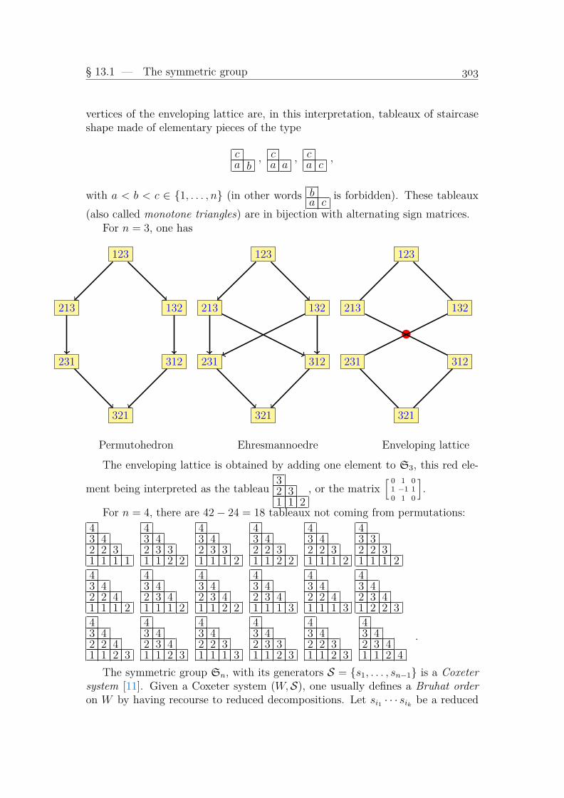
§ 13.1 — The symmetric group
vertices of the enveloping lattice are, in this interpretation, tableaux of staircaseshape made of elementary pieces of the type
ca b
, ca a
, ca c
,
with a < b < c ∈ 1, . . . , n (in other words ba c
is forbidden). These tableaux(also called monotone triangles) are in bijection with alternating sign matrices.
For n = 3, one has
123
213 132
231 312
321
123
213 132
231 312
321
123
213 132
•231 312
321
Permutohedron Ehresmannoedre Enveloping lattice
The enveloping lattice is obtained by adding one element to S3, this red ele-
ment being interpreted as the tableau32 31 1 2
, or the matrix[ 0 1 0
1 −1 10 1 0
].
For n = 4, there are 42− 24 = 18 tableaux not coming from permutations:43 42 2 31 1 1 1
43 42 3 31 1 2 2
43 42 3 31 1 1 2
43 42 2 31 1 2 2
43 42 2 31 1 1 2
43 32 2 31 1 1 2
43 42 2 41 1 1 2
43 42 3 41 1 1 2
43 42 3 41 1 2 2
43 42 3 41 1 1 3
43 42 2 41 1 1 3
43 42 3 41 2 2 3
43 42 2 41 1 2 3
43 42 3 41 1 2 3
43 42 2 31 1 1 3
43 42 3 31 1 2 3
43 42 2 31 1 2 3
43 42 3 41 1 2 4
.
The symmetric group Sn, with its generators S = s1, . . . , sn−1 is a Coxetersystem [11]. Given a Coxeter system (W,S), one usually defines a Bruhat orderon W by having recourse to reduced decompositions. Let si1 · · · sik be a reduced

Chapter 13 — Complements
decomposition of w ∈ W . Then v ≤ w with respect to the Bruhat order if andonly if there exists a reduced decomposition of v which is a subword of si1 · · · sik .
It is easy to check that two permutations σ, ζ are consecutive with respect tothe Bruhat order if and only if σζ−1 is a transposition. Therefore the Bruhatorder for the symmetric group coincides with the Ehresmann order. We shall usethe terminology Ehresmann-Bruhat order for it, and refering to [11] for moreproperties.
We have seen in Lemma 1.10.4 that 0-Hecke algebras give an easy way of gen-erating lower intervals for the Ehresmann-Bruhat order on classical Weyl groups.Stembridge [187] gives more generally a short derivation of the Möbius functionfor the Bruhat orderings of Coxeter groups and their parabolic quotients by usingthe 0-Hecke algebra.

§ 13.2 — t-Schubert polynomials
13.2 t-Schubert polynomialsThe spectral vectors for Macdonald polynomials specialize, in q = 1, into a per-mutation of [t0, t1, . . . , tn−1]. Let us show that one can similarly generalize thespectral vectors for Schubert polynomials by multiplying the components by apermutation of [t0, t1, . . . , tn−1].
Let v ∈ Nn be the code of a permutation σ. Let β ∈ Nn be such thatβi = #(σj < σi, i 6= j), that is, β and [σ1, . . . , σn] are two copies of the samepermutation in S(0, 1, . . . , n−1) and S(σ1, . . . , σn) respectively. Let more-over
〈vt〉 = [tβ1yσ1 , . . . , tβnyσn ] .
One defines the t-Schubert polynomial Y tv (x) by the condtions
Y tv
(〈ut〉
)= 0 for all u : |u| ≤ |v|, u 6= v ,
Y tv (x)
∣∣∣t=1
= Yv(x,y)(13.2.1)
These polynomials specialize, in t = 1, into the usual Schubert polynomi-als Yv(x,y), share many of their properties and constitute still another basis ofPol(xn).
Proposition 13.2.1. The family Y tv (x), v ∈ Nn is stable under ∂1, . . . , ∂n−1.
Let v = u+ kn, with k ∈ N. Then Y tv (x) = Ykn(x,y)
(Y tu(x)
∣∣yi→yi+k
).
Proof. Let v and i be such that vi > vi+1, and let u = [. . . , vi−1, vi+1, vi−1,vi+1, . . . ]. Then 〈ut〉 = 〈vt〉si, and the proof that Y t
ux) is equal to Y tvx)∂i is the
same than in the case t = 1.As for the factorization property of Y t
u+kn(x), the polynomial Y tv (x) does have
to satisfy more vanishing properties than Y tu(x), but the factor Ykn(x,y) takes
care of all the points w ∈ Nn having at least one component not greater than k.Thus, one is left with the vanishing in all points w ⊆ kn, |w| ≤ |v|, w 6= v, andthis is insured by the image of t-Schubert polynomial Y t
u(x) under the uniformtranslation of indices yi → yi+k. QED
As a consequence, t-Schubert polynomials are determined by the dominantones. However, contrary to the case of the usual Schubert polynomials, whenv is dominant, Y t
v (x) is not a product of linear factors in general. t-Schubertpolynomials indexed by antidominant weights are symmetrical in x1, . . . , xn, sincethey belong to the images of ∂1, . . . , ∂n−1.
Monk’s formula extends smoothly.
Lemma 13.2.2. Let w ∈ Nn, i be such that wi > 0, v be the image of w underwi → wi−1. Then there exists rational functions cu in t, y1, y2, . . . such that onehas
(xi − 〈vt〉i)(〈wt〉i − 〈vt〉i)
Y tw(〈wt〉)Y tv 〈wt〉
= Y tw(x) +
∑u: |u|=|w|, u 6=w
cuYtu(x) . (13.2.2)

Chapter 13 — Complements
Proof. Both sides of the equation are polynomials of degree |w| which vanish in allpoints 〈ut〉 : |u| < |w|. One can therefore determine the required coefficients cuby specializing the LHS in 〈ut〉 : |u| = |w|, u 6= w, to insure the equality of bothsides of the equation in maximal degree. QED
In the case of Schubert polynomials, the specialization Yv(〈v〉,y) is equalto the inversion polynomial e(v) =
∏(ji)∈Inv(σ)(yj − yi), with σ of code v. Let
[α1, . . . , αn] = [σ1, . . . , σn]↑, and
yv = [y1, . . . , yα1 , tyα1+1, . . . , tyα2 , . . . , tn−1yαn−1+1, . . . , t
n−1yαn ,
tnyαn+1, . . . , tny∞] .
Then we conjecture that
Y tv 〈wt〉 =
∏(ji)∈Inv(σ)
(yvj − yvi ) . (13.2.3)
Instead of expanding the basis Y tv (x) in the basis Yu(x,y), one rather
choose the bases Yu(x,yv) or Yu(x,yu) to obtain more compact expressions.For example
Y t012(x) = Y012(x,y012) +
(t− 1) (t2y4 + ty3 − ty2 − y1) y2
(t2y4 − y1) (ty3 − y1)Y111(x,y012) ,
with y012 = [y1, ty2, ty3, t2y4, t
2y5, t3y6, . . . ], while the expansion of Y t
012(x) in theSchubert basis involves
Y012(x,y), Y111(x,y), Y002(x,y), Y011(x,y), Y001(x,y), Y000(x,y) .
Contrary to the case of Schubert polynomials, one cannot concatanate 0 tothe right of v, since in general Y t
v 0(x) 6= Y tv (x). In fact, concatanating sufficiently
many 0’s gives back the Schubert polynomials, as shows the next lemma.
Lemma 13.2.3. Let v ∈ Nn, k ≥ |v|. Then
Y tv 0k(x) = Yv(x,y
v) .
Proof. One has to test vanishing in all u ∈ Nn+k, |u| ≤ |v|, u 6= [v, 0k]. Thepermutation σ of code u belongs to Sn+k and the spectral vector 〈ut〉 is the imageof 〈u〉 under yi → ti−1yi. Thus, the set of vanishing conditions is the set definingYv 0k(x,y
v). QED
For example, Y t2 (x) = (x1−y1)(x1−y2), Y t
20(x) = Y t2 (x)+ (t−1)y2
ty3−y1 (x1−y1)(x2−ty3),Y t
200(x) = (x1−y1)(x1−ty2).One can reduce the number of equations in the determination of Y t
v , v domi-nant, and avoid testing all u : |u| ≤ |v|, u 6= v, as show the next factorization.

§ 13.2 — t-Schubert polynomials
Lemma 13.2.4. Let v be dominant, v = [v1, . . . , vr, 0, . . . , 0] with vr > 0. Thenthere exist a polynomial Pv(x) of degree |v| − r such that
Y tv (x) = (x1−y1) . . . (xr−yr)Pv(x) ,
which is determined by the conditionsPv(〈ut〉
)= 0 for all u : u ≥ [1r0n−r], |u| ≤ |v|, u 6= v ,
Pv(x)∣∣∣t=1
= Yv(x,y)/Y1r(x,y) .(13.2.4)
Proof. One notices that (x1−y1) . . . (xr−yr) vanishes in all points 〈yt〉 such that0 ∈ u1, . . . , ur, because if ui = 0 is the first occurrence of 0 in u, then 〈ut〉i = y1.Therefore, it remains to satisfy the vanishing conditions for all points u >≥[1r, 0n−r], points that one can write w+[1r, 0n−r], with |w| ≤ |v|−r, w 6= v−[1r, 0n−r].QED
For example, Y t210 = (x1−y1)(x2−y2)P210(x), with
P210(x) = x100 +y2(t−1)
t2y4−y1
x001 − y2(t3y4−y1)
t2y4−y1
x000 ,
determined by the conditions
P210(〈110t〉) = 0 = P210(〈111t〉) = P210(〈120t〉) ,
P210(x)∣∣∣t=1
= Y210(x,y)/Y110(x,y) = x1 − y2 .
Notice that Y t100(x) is determined by similar conditions
Y t100(〈000t〉) = 0 = Y t
100(〈001t〉) = Y t100(〈010t〉) , Y t
100(x)∣∣∣t=1
= Y100(x,y)
but there is no change of variables which allows to pass from one system of equa-tions to the other.
It is interesting to specialize the variables yi to 1, but the specialized equations(13.2.4) are not sufficient to determine the specialization of Y t
v (x). For example,all the polynomials Y t
v (x)∣∣yi=1
, v ∈ N2, v 6= [0, 0], [1, 0] vanish in the points [1, t]
and [t, 1].One computes
Y t002(x)
∣∣yi=1
= (x1+x2+x3 − 1−t−t2)2
Y t012(x)
∣∣yi=1
= (x1+x2+x3 − 1−t−t2)S2(x1+x2+x3 − 1−t)
Y t022(x)
∣∣yi=1
= (S2(x1+x2+x3 − 1−t))2 .
This leads to the conjecture that the specialization yi = 1 of the symmetric poly-nomial Y t
v (x), v anti-dominant, coincides with the specialization q = 1 of theMacdonald polynomial Mv↓ seen in (??).

Chapter 13 — Complements
The non-symmetric case is more subtle. Let us write that a sum of Y tv is
equivalent to a sum of Macdonald polynomials if they become equal after special-ization yi → 1, q → 1 and reversal of the alphabet xi → xn+1−i in the Macdonaldpolynomials. Then one has Y t
320 ∼ M023, Y t302 ∼ M203, Y t
230 ∼ M032, Y t023 ∼ M320,
butY t
203 ∼M104 & Y t032 ∼M230 +
t2 − tt2 − 1
M203 .
§ 13.3 — Polynomials under C-action
13.3 Polynomials under C-actionWe have seen that Pol(xn) is a free Sym(xn)-module. More generally, the ring ofLaurent polynomials in xn is a free module over the invariants of the Weyl groupsof type Bn, Cn, Dn respectively. For a basis of monomials, in the more generalcase of a symmetrizable KacMoody group, in relation with the K-theory of theassociated flag variety, see the article of Griffeth and Ram [58, Th.2.9].
Let us give in this section an explicit description of Pol(xn) as a free moduleunder the action of the Weyl group W of type Cn.
As usual, we have to start with the smallest possible case, which is here, indisagreement with Bourbaki, n = 1.
We thus have polynomials in x1, x−11 , and the operator sC1 : x1 → x−1
1 . Tounderstand the underlying structure, we may rather use two indeterminates x, ysatisfying the relation xy = 1. Any polynomial f(x, y) can be written
f(x, y) = f1 + xf2, f1, f2 ∈ Sym(x, y) .
Indeed, f2 = f∂x,y and f1 = −yf∂x,y.In our case, this means that f(x1) = f1 + x1f2, with f1, f2 invariant under sC1 .
But a polynomial invariant under sC1 is a polynomial in the variable x•1 := x1+x−11 ,
and one may rephrase the preceding construction as
Lemma 13.3.1. Pol(x±1 ) is a free-module over Pol(x•1) = Sym(x•1) with basis1, x1.
As a corollary, one deduces
Lemma 13.3.2. Pol(xn) := Pol(x±1 , . . . , x±n ) is a free module over the ring of
usual polynomials Pol(x•n) := Pol(x•1, . . . , x•n), with basis xv : v ∈ 0, 1n.
In other words, the ring of Laurent polynomials, say in coefficients in C, maybe identified with the tensor product of the two-dimensional spaces 〈1, xi〉, i =1, . . . , n, with the ring of polynomials in x•1, . . . , x•n.
Choosing furthermore a basis of Pol(x•n) as a free Sym(x•n)-module and usingthe preceding lemma, furnishes a basis of Pol(x) as a module over itsW -invariants.For example, one can take the Schubert polynomials1 Xσ(x•,0), σ ∈ Sn, which,by definition, are all the different images of Xn...1(x•,0) := (x•1)n−1 · · · (x•n)0 underproducts of divided differences
∂•i := (1− si)1
x•i − x•i+1
= ∂i1
1− x−1i x−1
i+1
.
In summary, one has the following structure.1 It is more convenient to index the polynomials by permutations in Sn rather than by their
code.

Chapter 13 — Complements
Proposition 13.3.3. The ring of Laurent polynomials Pol(xn) is a free moduleover Sym(x•n), with basis
xvXn...1(x•,0) : v ∈ 0, 1n, σ ∈ Sn .
Since one has taken Schubert polynomials in x•n, it is natural to use thequadratic form
(f, g)C := fg ∂C1 · · · ∂Cn ∂•ω = fg x−ρC
πCw0. (13.3.1)
Since xi∂Ci = 1, 1∂Ci = 0, and Xσ(x•,0)∂•ω = 0, except Xω(x•,0)∂•ω = 1, it isimmediate to evaluate the scalar product of all the elements of the basis with 1 :
Lemma 13.3.4.(xvXσ(x•,0) , 1
)C= 0 except
(x1...1Xω(x•,0), 1
)C= 1 . (13.3.2)
Having a basis and a quadratic form, we have now to look for the adjoint basis,or equivalently, to look for a reproducing kernel.
Back to the case n = 1, this is achieved by taking an extra indeterminate y1.Then one instantly checks that 1, x1 − y1 and 1, y1 − x−1
1 are adjoint baseswith respect to (f, g)C = fg ∂C1 .
Thus it is appropriate to introduce indeterminates y1, . . . , yn, to use the poly-nomials (x1 − y1)v1 · · · (xn − yn)vn , v ∈ 0, 1n, instead of the monomials xv,and to use the Schubert polynomials Xσ(x•,y•) in the two alphabets x•, y• =(y1 +y−1
1 ), . . . , (yn+y−1n ). These polynomials are, by definition, all the different
images of
Xω(x•,y•) :=∏
i,j: i+j≤n
(x•i − y•j ) =∏
i,j: i+j≤n
(xi + x−1i − yj − y−1
j )
under products of divided differences ∂•i (which act only on x•).Let us choose an indexing compatible with the tensor product structure of
Pol(xn). Any element w of W is identified with a bar permutation (or signedpermutation). In other words, we write w ∈ W as
w = [(−1)ε1σ1, . . . , (−1)εnσn], with ε ∈ 0, 1n, σ ∈ Sn .
Let, for any w ∈ W , σ = [|w1|, . . . , |wn|], v ∈ 0, 1n such that vi = 1 whenever−i ∈ w. Define
XCw (x,y) = (x1 − y1)v1 · · · (xn − yn)vn Xσ(x•,y•) , (13.3.3)
XCw (x,y) = (−1)`(σ)
(y1−
1
x1
)v1· · ·(yn−
1
xn
)vnXσ((x•)ω,y•) . (13.3.4)
Notice that in the last Schubert polynomials, we have reversed the alphabetx• and used (x•)ω = [x•n, . . . , x
•1].
Knowing that, in the case of the usual ring of polynomials, (−1)`(σ)Xσ(xω,y)is the basis adjoint to the basis Xσ(x,y), with respect to the scalar product(f, g)∂ = fg∂ω, combining with the analysis for n = 1, one obtains

§ 13.3 — Polynomials under C-action
Theorem 13.3.5. The ring of Laurent polynomials Pol(xn) is a free module overSym(x•n), with pairs of adjoint bases XC
w (x,y) : w ∈ W and XCw (x,y) : w ∈
W. More precisely, let write −wω for [−wn, . . . ,−w1]. Then, for any w ∈ W ,one has (
XCw (x,y) , XC
−wω(x,y))C
= 1
and the other scalar products are 0.
For example, for n = 2, the two adjoint bases areXC
[(−1)ε11, (−1)ε22] = (x1 − y1)ε1 (x2 − y2)ε2 ,
XC[(−1)ε22, (−1)ε11] = (x1 − y1)ε1 (x2 − y2)ε2
(x•1 − y•1
), ε1, ε2 ∈ 0, 1
,
XC
[(−1)ε11, (−1)ε22] = (y1 −1
x1
)ε1 (y2 −1
x2
)ε2 ,
XC[(−1)ε22, (−1)ε11] = (y1 −
1
x1
)ε1 (y2 −1
x2
)ε2(y•1 − x•2
), ε1, ε2 ∈ 0, 1
.
The second alphabet y may be thought as a set of arbitrary parameters. Onemay “specialize” it to 0, i.e. specialize all yi to 0 in the linear factors occurring inthe expression of XC
w (x,y) and XCw (x,y), as well as specializing all y•i to 0 inside
the Schubert polynomials.Notice that Weyl’s character formula for type C uses the operator πCw0
whichis equal to xn1 · · ·x1
n ∂C1 · · · ∂Cn ∂•ω. Weyl’s formula xλ πCw0
= Spλ(xn) may be written(xλ , xn1 · · ·x1
n) = Spλ(xn).Key polynomials for type C may be written as linear combinations ofXC
w (xn,0)with coefficients expressed in terms of symplectic Schur functions. For example,for n = 2, writing Xw instead of XC
w (x2,0), and Spλ instead of Spλ(x2), one has
KC−3,1 = Sp2
(X−2,1 −X2,−1 −X−1,−2
)− Sp11X1,2 + Sp1Sp2X−1,2 .
As in the case of type A, it is not difficult to reformulate the preceding con-struction of pairs of adjoint bases in terms of a kernel.
Theorem 13.3.6. Let
Θn(x,y) :=n∏i=1
(xi −
1
yi
)∏i<j
(xi +
1
xi− yj −
1
yj
).
Then Θn(x,y) is a reproducing kernel, modulo the identification Sym(x•) = Sym(y•),i.e. one has
∀f ∈ Pol(x) ,(f(x1, . . . , xn) , Θn(x,y)
)∣∣∣x=y
= f(y1, . . . , yn) . (13.3.5)

Chapter 13 — Complements
Proof. Writing the scalar product as a summation over W , thanks to (1.10.4), theLHS becomes (∑
±fwΘn(xw,y)) 1
∆C
∣∣∣x=y
.
However, all Θn(xw,y) vanish under the specialization x = y, i.e. x1 = y1, . . . , xn =yn, but when w is the identity, in which case Θn(y,y) = ∆C(y). QED
The quadractic form takes values in Sym(x•) and is Sym(x•)-bilinear, thisforces the identification of Sym(x•) with Sym(y•).
The kernel diagonalizes into any pair of adjoint bases. For example, given anyz = z1, z2, writing Xw for XC
w (x, z) and writing Xw for XCw (y, z), one may check
directly for n = 2 that
Θ2(x,y) =
(x1 −
1
y1
)(x2 −
1
y2
)(x1 +
1
x1
− y2 −1
y2
)= X1,2X−2,−1 +X−1,2X−2,1 +X1,−2X2,−1 +X−1,−2X2,1 +X2,1X−1,−2
+X2,−1X1,−2 +X−2,1X−1,2 +X−2,−1X1,2 .
§ 13.4 — Polynomials under D-action
13.4 Polynomials under D-actionThere are more functions which are invariant under D-action than C-action. Forexample, for n = 2, x1 + x−1
2 is invariant under s1, sD2 , hence is a D-invariant, but
it is not invariant under sC2 .To describe Pol(xn) as a module over the ring SymD(n) ofD-invariant, one can
start from the C-basis XCw (xn,0). However, we shall see that polynomial coef-
ficients are not sufficient. Thus, one defines SymD(n) to be the ring of symmetricrational functions in x±1 , . . . , x±n which are invariant under sDn .
Adapting the type C-case, one takes the quadratic form
(f, g)D = fg x−ρD
πDw0= fgθDn ∂
•ω , (13.4.1)
using the notation of (1.10.6).The Weyl group of type D may be considered as the subgroup of signed per-
mutations with an even number of signs. This embedding WDn → WC
n does notpreserve the pairing:
(XC−2,−1(xn,0), XC
12(xn,0))C = 1 , (XC−2,−1(xn,0), XC
−1,−2(xn,0))C = 0, . . .
but
(XC−2,−1(xn,0), XC
12(xn,0))D = x1x2+x−11 x−1
2 , , (XC−2,−1(xn,0), XC
−1,−2(xn,0))D = 2 , . . .
To show nevertheless that XCw (xn,0) : w ∈ WD
n is a SymD(n)-basis, one usesanother quadratic form
((f, g))D = (f, g)D ∩(KD−1,...,−1 −KD
−1,...,−1,1
),
the notation meaning that, after expressing (f, g)D in the KD basis, that is,(f, g)D = aKD
−1,...,−1 + bKD−1,...,−1,1 + · · · , one puts ((f, g))D = a− b.
The next lemma, which is immediate to verify, shows that the two specialkey-polynomials KD
−1,...,−1, KD−1,...,−1,1 occur in the images of monomials under θDn .
Lemma 13.4.1. Let v ∈ −1, 0, 1n, m(k) be the number of components of v equalto k. Let u = [|v1|, . . . , |vn|], ε = (−1)n+m(−1)+1. Then
xvθDn =
KD
(−1)n−1,ε−KD
(−1)n−2,02+KD(−1)n−4,04− · · · if m(0) = 0
2m(0)−1(x•)u if m(0) > 0 .(13.4.2)
Proposition 13.4.2. For w,w′ ∈ WCn , one has((
XCw (xn,0) , (−1)nXC
w′(xn,0)))D
= δw′,−wω . (13.4.3)
Consequently, the set XCw (xn,0) : w ∈ WD
n is a SymD(n)-basis.

Chapter 13 — Complements
Proof. The product of the two polynomials XCw , Xw′ is equal to the product of
two Schubert polynomials in x• times a monomial xv, with v ∈ −1, 0, 1n. If vhas at least a component equal to 0, then its image under θDn is a monomial inx•. This monomial, multiplied by the two Schubert polynomials belongs to thespan of monomials (in x•) of exponent ≤ [n, . . . , n]. It image under ∂•ω belongsto the span of Schubert polynomials Y0n−i,1i(x
•,0). If i 6= n, then Y0n−i,1i(x•,0)
has no component in the KD-basis of index [(−1)n−1,±1]. Moreover Y1n(x•,0) =x•1 · · ·x•n = KD
(−1)n + K(−1)n−1,1 + · · · . Therefore, to avoid nullity, v must haveno component equal to 0. But in that case xvθDn is D-invariant and commuteswith ∂•ω. One is reduced to the case of two Schubert polynomials (2.6.6), and thisallows to conclude. QED
To expressXCw (xn,0), when w ∈ WC
n \WDn , in the above basis is not immediate.
For example, for n = 2, writing w instead of XCw (xn,0), Kv instead of KD
v , puttingγ = (x1x2 − x−1
1 x−12 )2, one has the following expansions
[12] [12] [21] [21]
γ[12] K21 −2K10 −K11−K00 K11+K00
γ[12] −2K10 K21 K11+K00 −K11−K00
γ[21] −K22−K20−K11+K00 K22+K20+K11−K00 K21 −2K10
γ[21] K22+K20+K11−K00 −K22−K20−K11+K00 −2K10 K21

§ 13.5 — Hecke algebras of types B,C,D
13.5 Hecke algebras of types B,C,DIn type A, we have obtained the Hecke algebra by replacing the simple trans-positions si by Ti = (t1 + t2)πi − t2si. Having at our disposal π♥n and s♥i for♥ = B,C,D, we have therefore candidates for T♥n . One can in fact take indepen-dent parameters for types B and C. We prefer to rename the parameters for typeA, and define for i ≥ 1,
Ti = (q1+q2)πi − q2si & TBi = (t1+t2)πBi − t2sBi & TCi = (t1+t2)πCi − t2sCi ,
and, for i ≥ 2,TDi = (q1+q2)πDi − q2s
Di .
These operators satisfy the braid relations, together with
(TBi − t1)(TBi − t2) = 0, (TCi − t1)(TCi − t2) = 0, (TDi − q1)(TDi − q2) = 0 .
The collection T1, . . . , Tn−1, T♥n generates the Hecke algebra of type ♥ = B,C,D.
One can order differently the Dynkin graph. In type C, instead of usingthe divided difference relative to the pair xn, x−1
n , one takes the pair x−11 , x1, and,
correspondingly, πC0 = πx−11 ,x1
, and sC0 = sC1 . In type B, one takes πB0 = πx−1/21 ,x
1/21
,and sB0 = sB1 . In type D, one puts sD0 = sD2 ,
f(x1, x2, . . . ) πD0 =
(x−1
1 x−12 f − f sD0
)(x−1
1 x−12 − 1)−1 .
Thus
TB0 = (t1+t2)πB0 − t2sB0 & TC0 = (t1+t2)πC0 − t2sC0 & TD0 = (q1+q2)πD0 − q2sD0 .
The operators TB0 , TC0 are characterized by the fact that they commute withthe functions of x•1 = x1 + x−1
1 , and by the images of 1, x1, which are
1TB0 = t1 = 1TC0 , x−11 TB0 = −t1−t2−t2x
−11 , x−1
1 TC0 = t2x−11 .
The operator TD0 is characterized by the fact that it commutes with functionswhich are invariant under sD0 , and by the images of 1, x1, x2, x2x
−11 , which are
1TD0 = q1, x1TD0 = −q2x
−12 , x2T
D0 = −q2x
−11 , x2x
−11 TD0 = q1x2x
−11 .
The set T♥0 , T1, . . . , Tn−1 generates another realization of the Hecke algebraof type ♥, as an algebra of operators on polynomials. This is this realization thatwe shall retain in this section.
One can, of course, combine both realizations, or use simultaneously the op-erators for the different types. From the explicit images of 1, x1, x2, x2x
−11 , one
discovers that TD0 coincides with the specialization t1 = 1, t2 = −1 of TC0 T1TC0 .
Thus, the Hecke algebra of type D may be obtained as a subalgebra of the Heckealgebra of type C for t1 = 1, t2 = −1.

Chapter 13 — Complements
As for type A, inserting parameters in the braid relations is a powerful wayof obtaining interesting elements of the Hecke algebra. We refer to the workof Cherednik [21, 22, 23] for a Yang-Baxter philosophy and its application tomathematical physics. For our part, we shall restrict to the construction of Yang-Baxter graphs for the Hecke algebras of the Weyl groups, wich allow to insertparameters inside reduced decompositions in a coherent way.
A Yang-Baxter graph is a graph with vertices labelled by pairs Yw, v, w in theWeyl group W♥,n, v a vector of length n, satisfying the following conditions.
The starting point is the pair consisting of 1 = Y12...n and of an arbitraryspectral vector. The other elements are recursively defined by the same rule thanin type A, which is, for i > 0,
(Yw, v
)→(Yw(Ti +
q1 + q2
vi+1v−1i − 1
), vsi
)when `(wsi) > `(w) , (13.5.1)
the rule for type D being
(Yw, v
)→(Yw(TD0 +
q1 + q2
v1v2 − 1
), vsD0
)when `(wsD0 ) > `(w) , (13.5.2)
and finally, the rule for type ♥ = B,C being
(Yw, v
)→(Yw(T♥0 +
t1 + t2v2
1(−t1t2)−1 − 1
), vs♥0
)when `(ws♥0 ) > `(w) , (13.5.3)
with vsB0 = vsC0 = [−t1t2v−11 , v2, . . .] and vsD0 = [v−1
2 , v−11 , v3, . . .].
The fact that the elements Yw are well defined translates algebraically in theYang-Baxter equations for types B,C,D. The relation sD0 s2s
D0 = s2s
D0 s2 corresponds
to an embedding of S3 into WD,3, thus comes from type A. Thus, there is onlyone new relation, which is for type C (or B). On the following graphical display,this relations translates into the fact that the two paths from top to bottom giveequal elements in the Hecke algebra (each path being evaluated as the product ofthe labeling of its edges).
Write pairs w, Ti(γ) instead of YCw , Ti+ t1+t2γ−1
, for the vertices of the Yang-Baxtergraph.
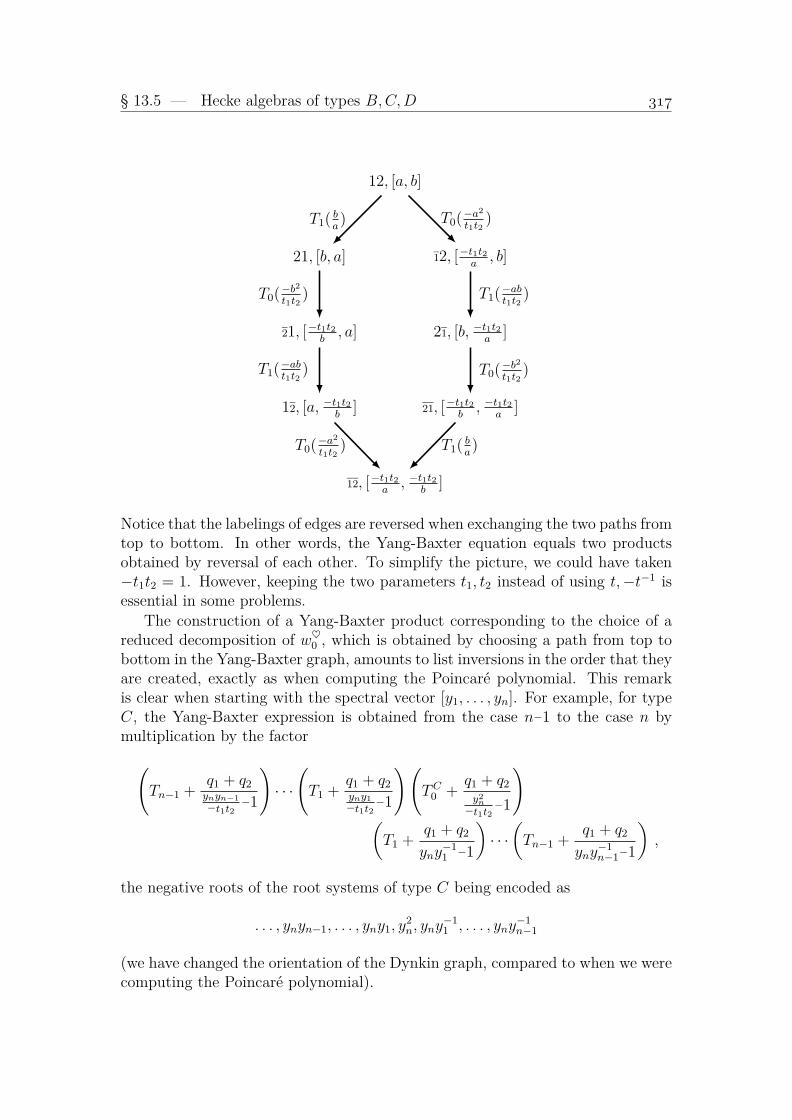
§ 13.5 — Hecke algebras of types B,C,D
12, [a, b]
21, [b, a] 12, [−t1t2a, b]
21, [−t1t2b, a] 21, [b, −t1t2
a]
12, [a, −t1t2b
] 21, [−t1t2b, −t1t2
a]
12, [−t1t2a, −t1t2
b]
T1( ba) T0(−a
2
t1t2)
T0(−b2
t1t2)
T1(−abt1t2
)
T0(−a2
t1t2)
T1(−abt1t2
)
T0(−b2
t1t2)
T1( ba)
Notice that the labelings of edges are reversed when exchanging the two paths fromtop to bottom. In other words, the Yang-Baxter equation equals two productsobtained by reversal of each other. To simplify the picture, we could have taken−t1t2 = 1. However, keeping the two parameters t1, t2 instead of using t,−t−1 isessential in some problems.
The construction of a Yang-Baxter product corresponding to the choice of areduced decomposition of w♥0 , which is obtained by choosing a path from top tobottom in the Yang-Baxter graph, amounts to list inversions in the order that theyare created, exactly as when computing the Poincaré polynomial. This remarkis clear when starting with the spectral vector [y1, . . . , yn]. For example, for typeC, the Yang-Baxter expression is obtained from the case n−1 to the case n bymultiplication by the factor(
Tn−1 +q1 + q2ynyn−1
−t1t2−1
)· · ·
(T1 +
q1 + q2yny1−t1t2
−1
)(TC0 +
q1 + q2
y2n−t1t2
−1
)(T1 +
q1 + q2
yny−11 −1
)· · ·(Tn−1 +
q1 + q2
yny−1n−1−1
),
the negative roots of the root systems of type C being encoded as
. . . , ynyn−1, . . . , yny1, y2n, yny
−11 , . . . , yny
−1n−1
(we have changed the orientation of the Dynkin graph, compared to when we werecomputing the Poincaré polynomial).

Chapter 13 — Complements
The alternating sum 1|W |
∑w(−1)`(w)w on a Weyl group is a fundamental idem-
potent. We have seen (1.9.10 ) how fruitful it is in type A to factorize the corre-sponding element of the Hecke algebra. Let us do the same for types B,C,D.
In type ♥ = B,C, instead of the usual length, one defines `0(w) (resp. `1(w))to be the degree in s♥0 (resp. in s1, s2, . . .) of any reduced decomposition of w. Let
∇♥,n =∑
w∈W(−t1)n−`0(w)(−q1)n(n−1)−`1(w) Tw , ♥ = B,C , (13.5.4)
∇D,n =∑
w∈W(−q1)n(n−1)−`(w) Tw (13.5.5)
The description of the canonical reduced decompositions of the elements of theWeyl groups of type ♥ = B,C,D entails the following factorizations of the sums∇♥,n:
∇♥,n = ∇♥,n−1(Tn−1 · · ·T♥0 · · ·Tn−1 − q1Tn−1 · · ·T♥0 · · ·Tn−2 + · · ·
+ (−q1)n−1Tn−1 · · ·T♥0 − t1(−q1)n−1Tn−1 · · ·T1 + · · ·
− t1(−q1)2n−3Tn−1 − t1(−q1)2n−2), ♥ = B,D . (13.5.6)
∇D,n = ∇D,n−1(Tn−1 · · ·T2T
D0 T1 · · ·Tn−1 + · · ·+ (−q1)n−2Tn−1 · · ·T2T
D0 T1
+ (−q1)n−1Tn−1 · · ·T2TD0 + (−q1)n−1Tn−1 · · ·T2T1
+ (−q1)nTn−1 · · ·T2 + · · ·+ (−q1)2n−2)
(13.5.7)
However, ∇♥,n is a Yang-Baxter element, as shows the following proposition.
Proposition 13.5.1. For types B,C,D, ∇♥,n is the bottom element of the Yang-Baxter graph corresponding to the spectral vectors [t2, (−q2q
−11 )t2, . . . , (−q2q
−11 )n−1t2]
for types B,C, and [1, −q2q−11 , . . . , (−q2q
−11 )n−1] for type D.
In particular, one has the following factorizations, for types ♥ = B,C,
∇♥,n = ∇♥,n−1
Tn−1 +q1 + q2
−t2t1
(−q2q1
)2n−3−1
· · ·T1 +
q1 + q2
−t2t1
(−q2q1
)n−1−1
TC0 +
q1 + q2
−t2t1
(−q2q1
)2n−2
− 1
T1 +
q1 + q2(−q2q1
)n−1
− 1
· · ·(Tn−1 +q1 + q2−q2q1− 1
), (13.5.8)

§ 13.5 — Hecke algebras of types B,C,D
and for type D,
∇D,n = ∇D,n−1
Tn−1 +q1 + q2(−q2q1
)2n−3−1
· · ·T2 +
q1 + q2(−q2q1
)n−1
TD0 +
q1 + q2(−q2q1
)n−1−1
T1 +
q1 + q2(−q2q1
)n−1−1
T2 +
q1 + q2(−q2q1
)n−2
− 1
· · ·(Tn−1 +q1 + q2−q2q1− 1
). (13.5.9)
Proof. Using the Yang-Baxter relations, one can factor on the left of the righthand-side of the two above expressions each of the simple factors (T1−q1), . . .,(Tn−1−q1), and TD0 −q1) or (T
B/C0 −t1). Moreover, the term of maximal length is
T♥w0. Therefore these factorized expressions are equal to the quasi-idempotents
∇♥,n. QEDFor types B,C, there are other factorizations which do not correspond to the
choice of a spectral vector, but present the advantage of having the parameterst1, t2 appear in only the factors containing T0.
Recall the notation (1.9.1) Ti(−k) = Ti − qk1/[k] for type A, with [k] = qk−11 −
q2qk−21 + · · · +(−q2)k−1. Let
βk = t1 +[k−1]
[k](t1q2+t2q1) , T♥0 (−k) = T♥0 −βk for k ≥ 1 , ♥ = B,C . (13.5.10)
Then one proves as above the following factorization of ∇B/C .
Proposition 13.5.2. For type ♥ = B,C, one has
∇♥,n = ∇♥,n−1 Tn−1(−n+1) · · ·T1(−1)T♥0 (−n)T1(−n+1) · · ·Tn−1(−1) . (13.5.11)
For example,
∇C,2 = (TC0 −t1)(T1−q1)
(TC0 − t1−
t1q2 + t2q1
q1 − q2
)(T1−q1)
= TC0 T1TC0 T1 − q1T
C0 T1T
C0 − t1T1T
C0 T1 + t1q1T
C0 T1 + t1q1T1T
C0
− t21q1T1 − t1q21T
C0 + t21q
21 .
All ∇♥,n, ♥ = A,B,C,D, are quasi-idempotents. As in the case of Weyl’scharacter formula, they send xρ♥ to a generalization of the Vandermonde.
Let
V A,n =∏
1≤i<j≤n
(q2xi + q1xj) & V D,n =∏
1≤i<j≤n
(q2xi + q1xj)
(q1 +
q2
xixj
),

Chapter 13 — Complements
V B,n = V D,n
n∏i=1
(t2√xi
+ t1√xi
)& V C,n = V D,n
n∏i=1
(t2xi
+ t1xi
).
The following theorem shows that V ♥,n is a right factor of ∇♥,n.
Theorem 13.5.3. With the notations of Propositions 1.10.1, 1.10.2, one has, for♥ = B,C,D,
∇♥,n = x−ρ♥π♥w0
V ♥,n (13.5.12)
=
(∑w
(−1)`(w)w
)V ♥,n
(∆♥,n
)−1 (13.5.13)
Moreover, for ♥ = B,C, one has
(−1)(n+1
2 )∇♥,n = ∂♥1 · · · ∂♥n ∂•ω V ♥,n = ∂•ω ∂♥1 · · · ∂♥n V ♥,n (13.5.14)
Proof. For each type, the different assertions are equivalent, thanks to the differentfactorizations of the maximal divided difference. Let us test (13.5.8), for type C,on the basis Pv,σ = xvXσ(x•n,0) : v ∈ 0, 1n, σ ∈ Sn of Pol(xn) as a freemodule over the invariant under C, defined in (13.3.3).
If v1 = 0, then Pv,σ is sent to 0 by ∂C1 , as well as by TC0 − t1, which is aleft factor of ∇C,n. Since σ∇C,n = (−1)`(σ)∇C,n for any permutation σ, non-vanishing implies that v = [1, . . . , 1]. Since ∂ω is a left factor of ∇A,n, henceof of ∇C,n, as well as of ∂•ω, non-vanishing requires that σ = ω. The imageof x1...1Xω(x•n,0) under the right-hand side of (13.5.8) is V C,n. The image under∇C,n is a polynomial f which belongs to the linear span of monomials of exponentsu such that [|u1|, . . . , |un|] ↓≤ [n, . . . , 1]. Since moreover ∇C,nTi = ∇C,nq2 fori = 1, . . . , n−1, and ∇C,nTC0 = ∇C,nt2, then f must be equal to V C,n, up to anon-zero constant. One finds this constant by computing, in the image of x1,2,...,n,the coefficient of 1/x1,...,n, which is (−tn2 )q
n(n−1)2 under TCw0
(hence under ∇C,n),and (−1)(
n2)tn2q
n(n−1)2 under the right-hand side. This settles the case of type C,
the case of type B being similar. The case D requires checking only the imagesof Pv,σ for v having an even number of components equal to 1. QED
For example,
−∇2,C = ∂C1 ∂C2 ∂•21 (q2x1 + q1x2)
(q1 +
q2
x1x2
)(t2x1
+ t1x1
)(t2x2
+ t1x2
).
Exchanging t1, t2, q1, q2, one obtains another family of quasi-idempotents
d♥,n =∑
w∈W(−t2)n−`0(w)(−q2)n(n−1)−`1(w) Tw , ♥ = B,C , (13.5.15)
dD,n =∑
w∈W(−q2)n(n−1)−`(w) Tw . (13.5.16)
This exchange of parameters give for d♥,n relations corresponding to (13.5.6),(13.5.7), (13.5.8), (13.5.9), taking factors Ti(k) = Ti − qk2(qk−1
2 + · · · +(−q1)k−1)−1
instead of Ti(−k).

§ 13.5 — Hecke algebras of types B,C,D
However, change of parameters is not sufficient for what concerns the expres-sion of d♥,n in terms of divided differences. One must also change the order ofoperations, as we have seen in type A. Let V ♥,n be the image of V ♥,n under thesymmetry q1 ↔ q2, t1 ↔ t2. Then one has
Theorem 13.5.4. Given n, let εA = 1, εB = εC = (−1)(n+1
2 ), εD = (−1)(n2). Then
d♥,n = ε♥V ♥,nx−ρ♥π♥w0
= V ♥,n∇♥,n(V ♥,n
)−1. (13.5.17)
For example,
dC,2 = − (q1x1+q2x2)
(q2+
q1
x1x2
)(t1x1
+t2x1
)(t1x2
+t2x2
)1
x21x2
πC0 π1πC0 π1 .
We have used the simultaneous transposition of t1, t2, and q1, q2. In type C(or B), one has two other ways to produce a quasi idempotent from ∇C , usinga single transposition. Let
(∇C,n
)(t2,t1) (resp.(∇C,n
)(q2,q1)) be the image of ∇C,n
under the transposition (t2, t1) (resp. (q2, q1)). Write V C,n(q1, q2, t1, t2) = V C,n,V C,n(q1, q2, ∅) = V D,n, V C,n(∅, t1, t2) =
∏ni=1
(t2xi
+t1xi
). We have just seen that
dC,n = ε♥V C,n(q2, q1, t2, t1)x−ρ♥πCw0
. The following proposition shows that the twoother quasi idempotents similarly factorize in terms of divided differences.
Proposition 13.5.5. Defining εC = (−1)(n+1
2 ) as in (13.5.17), using the factor-ization (1.10.3) of πCw0
, one has(∇C,n
)(q2,q1)= εCV C,n(q2, q1, ∅) ∂C1 · · · ∂Cn ∂•ω V C,n(∅, t1, t2) (13.5.18)(
∇C,n)(t2,t1)
= εCV C,n(∅, t2, t1) ∂C1 · · · ∂Cn ∂•ω V C,n(q1, q2, ∅) . (13.5.19)
For example,(∇C,2
)(t2,t1)= (TC0 −t2)(T1T
C0 +t2q1)(T1 − q1)
= (TC0 − t2)(T1 − q1)
(TC0 −
q1(t1+t2)
q1−q2
)(T1 − q1)
= −(t1x1
+ t2x1
)(t1x2
+ t2x2
)∂C1 ∂
C2 ∂•21 (q2x1 + q1x2)
(q1 +
q2
x1x2
).
Thus
−x1
(∇C,2
)(t2,t1)=
(x1
(t1x1
+ t2x1
)∂C1
)((t1x2
+ t2x2
)∂C2
)∂•21V
C,2(q1, q2, ∅)
= (t2(x1 + x−11 ))(t2 − t1)∂•21V
C,2(q1, q2, ∅) = t2(t2 − t1)V C,2(q1, q2, ∅) ,
value which would be more complicated to obtain using the definition(∇C,2
)(t2,t1)=∑
w∈W (−t2)n−`0(w)(−q1)n(n−1)−`1(w) Tw.

Chapter 13 — Complements
The Hecke algebraHDn contains two copies ofHA
n , one generated by T1, T2, . . . ,Tn−1, the other by TD0 , T2, . . . , Tn−1. However, these two copies act differentlyon polynomials. In fact, the identity sC0 T
D0 s
C0 = T1 exchanges the two actions.
Thus,
∇A,3 = T1(−1)T2(−2)T1(−1) = ∂321 (q2x1+q1x2) (q2x1+q1x3) (q2x2+q1x3)
entails
TD0 (−1)T2(−2)TD0 (−1) = sC0 ∂321sC0
(q2
x1
+q1x2
)(q2
x1
+q1x3
)(q2x2+q1x3) .
Since the work of Young, one knows that 1-dimensional idempotents are theelementary bricks with which to build representations of the symmetric group,and, by extension, of the Hecke algebras of the classical groups.
Due to the factorization (13.5.12), one can also use polynomials of the typeV ♥,n (c.f. [111] in type A). We have seen in the preceding chapters the im-portance of Yang-Baxter graphs to generate families of polynomials or bases ofrepresentations. Essentially, to describe a representation of the group algebra, orof the Hecke algebra of the fundamental groups, one needs a starting element. Anappropriate graph will take care of generating a basis from this element.
For example, in the case of the group algebra of the symmetric group, onecan start from a product of Vandermonde determinants on blocks of consecutivevariables to generate a “Specht module”. Standard Young tableaux index theelements of the Specht or Young basis, the starting element being indexed by thetableau having its columns filled with consecutive integers. Thus, one has to findsimilar “first elements” to generate representations of the different Hecke algebrasassociated to the classical groups.
Young orthogonal bases are nowadays characterized as eigenvectors of Jucys-Murphy elements [69, 154, 163]. In that respect, the fundamental property ofthe polynomial ∆t1,t2
λ encoutered in (1.9.14) is that it is an eigenvector of theJucys-Murphy elements ξA1 = 1, ξA2 = T1T1/(−q1q2), ξA3 = T2T1T1T2/(q1q2)2, . . .
Jucys-Murphy elements are recursively defined [172] by
ξA1 = 1, ξB1 = TB0 , ξC1 = TC0 , ξ
D2 = TD0 T1, ξ
♥i = Ti−1ξ
♥i−1Ti−1(−q1q2)−1 .
Irreducible representations of the Hecke algebra of type C are indexed bypairs of partitions, and, correspondingly, bases are indexed by bitableaux (pairsof standard tableaux). Representations may be realized as subspaces of the Heckealgebra, the elements corresponding to bitableaux being eigenvectors of the Jucys-Murphy elements with special eigenvalues [172]. According to what we have said,to obtain irreducible polynomial representations of the Hecke algebra HC
n , we needonly to exhibit, for each pair of partitions (λ, µ) : |λ|+|µ| = n, a polynomial whichis an eigenvector of the Jucys-Murphy elements, with the same eigenvalues as thebitableau of shape (λ, µ) filled with consecutive numbers in columns.

§ 13.5 — Hecke algebras of types B,C,D
We do not have a solution in general, but only in the case where [λ, µ] is apartition. We give without proof these polynomials, to prompt a reader to describethe general case.
Given three positive integers a, b, k, with a < b, let
φ(a, b, k) =∏
a≤i<j≤b
(q2xi + q1xj)
(qk1 −
(−q2)k
xixj
)(13.5.20)
φC(a, b, k) = φ(a, b, k)b∏i=a
(t2x−1i + t1xi
)(13.5.21)
Thus φC(1, n, 1) = V C,n.To a pair of partitions λ = [λ1, . . . , λr], µ = [µ1, . . . , µ`], one associates a
content-vector of length λ|+|µ|
c(λ, µ) =[[0, −1, . . . , −λ1+1], [1, 0, . . . , −λ2+2], . . . , [r−1, . . . , −λr+r],
[0, −1, . . . , −µ1+1], [1, 0, . . . , −µ2+2], . . . , [`−1, . . . , −λ`+`]]
(this vector is made of blocks that we have figured, one should erase the inside “[”and “]”).Claim. Let λ = [λ1, . . . , λr], µ = [µ1, . . . , µ`] be two partitions, with λ|| = mλ|+|µ| = n, such that λr ≥ µ1. Let c = c(λ, µ) be the content-vector, and
v = [λ1, λ1+λ2, . . . , λ1+ · · · +λr, λ1+ · · · +λr+µ1, . . . , λ1+ · · · +µ`] .
Then the polynomial
φC(1, v1, 1)φC(v1+1, v2, 2) · · ·φC(vr−1+1, vr, r)φ(vr+1, vr+1, r+1) · · ·φ(vr+`−1, vr+`, r+`)
is an eigenvector for the Jucys-Murphy elements ξC1 , . . . , ξCn with eigenvalues
t2, t2(−q1/q2)c2 , . . . , t2(−q1/q2)cm , t1, t1(−q1/q2)cm+2 , . . . , t1(−q1/q2)cn .
For example, for λ = [3, 2], µ = [2], the content-vector is c = [0, −1, −2, 1, 0, 0, −1]and the polynomial
(q2x1 + q1x2)
(q1 +
q2
x1x2
)(q2x1 + q1x3)
(q1 +
q2
x1x3
)(q2x2 + q1x3)(
q1 +q2
x2x3
)(t2x1
+ t1x1
)(t2x2
+ t1x2
)(t2x3
+ t1x3
)(q2x4 + q1x5)(
q12 − q2
2
x4x5
)(t2x4
+ t1x4
)(t2x5
+ t1x5
)(q2x6 + q1x7)
(q1
3 +q2
3
x6x7
).
is an eigenvector of the Jucys-Murphy elements, with eigenvalues
t2, −t2q2/q1, t2q22/q
21, −t2q1/q2, t2, t1, −t1q2/q1 .

Chapter 13 — Complements
13.6 Noncommutative symmetric functionsWe have already used noncommutative methods in the theory of symmetric func-tions, by embedding the ring Sym into Plac. Since Sym(x∞,) is a ring of polynomi-als in S1, S2, . . . , one can use another approach to noncommutativity by decidingthat S1, S2, . . . do not commute any more, and look for the bases analogous tothe bases of Sym other than products of complete functions.
Instead of using quasi-determinants as in [52], let us adopt a more down-to-earth point of view, and use a combinatorics of compositions2.
Given a composition v of n, let D(v) = [v1, v1+v2, . . . , v1+v2+ . . . +vr−1] =[d1, . . . , dr−1] be the list of descents of v, and 〈v〉 ∈ Nn−1 be the exponent ofthe monomial xd1 . . . xdr−1 .
Let Pol1 be the vector space with basis x〈v〉 indexed by all compositions,and Pol1n the subspace corresponding to compositions of n. Define the product
Pol1n ×Pol1m 3 f × g→ f(x1, . . . , xn−1) (1 + xn) g(x1+n, . . . xn+m−1) ∈ Pol1m+n .
Let Sym be the free associative algebra generated by S[1], S[2], . . .. Given anycomposition v = [v1, . . . , vr], denote S[v] the product S[v1] · · ·S[vr], and let Symn
be the linear span of S[v] : |v| = n.Other bases of Symn have been defined in [52] through generating functions.
Let σ(t) =∑
k≥0 tkS[k]. Then one defines L[k],Ψ[k],Φ[k] by∑
k≥0
tkL[k] = σ(−t)−1 (13.6.1)
∑k≥1
tk−1Φ[k] =d
dtlog(σ(t)
)(13.6.2)
∑k≥1
tk−1Ψ[k] = σ(t)−1 d
dtσ(t) . (13.6.3)
By product, one obtains three linear bases of Sym:
L[v] = L[v1]L[v2] . . . , Φ[v] = Φ[v1]Φ[v2] . . . , Ψ[v] = Ψ[v1]Ψ[v2] . . . .
Another important basis, the basis of ribbon functions R[v], is recursively definedby R[k] = S[k],
R[v, a]R[b, w] = R[v, a, b, w] +R[v, a+b, w] , a, b ∈ N+ .
One can identify Sym and Pol1 by sending S[k] to 1, and requiring the com-patibility with the product. In more details, let θ : Sym → Pol1 be defined byθ(S[k]) = 1 for all k ∈ N, and, for any two compositions v, w,
θ(S[v]S[w]) = θ(S[v]) (1 + x|v|) θ(S[w]) .
2In [52], one mostly uses quasi-determinants of almost triangular matrices (i.e. null underthe subdiagonal), in which case the theory is simpler than the general theory.

§ 13.6 — Noncommutative symmetric functions
Thus, given v = [v1, . . . , vr], let D(v) = [d1, . . . , dr−1] be the descents of v. Then
θ(S[v1, . . . , vr]
)= (1 + xd1)(1 + xd2) . . . (1 + xdr−1) (13.6.4)
θ(R[v1, . . . , vr]
)= xd1xd2 . . . xdr−1 = x〈v〉 . (13.6.5)
It is easy to check that
θ(L[k]) = x1 . . . xk−1 (13.6.6)θ(Ψ[k]) = 1− x1 + x1x2 − · · ·+ (−1)k−1x1 . . . xk−1 . (13.6.7)
A little more effort is required to show that
θ(Φ[k]) = 1−(k−1
1
)−1
e1 +
(k−1
2
)−1
e2 − · · ·+ (−1)k−1ek−1 , (13.6.8)
where e1, . . . , ek−1 are the elementary symmetric functions in x1, . . . xk−1.The above values induce θ(L[v]), θ(Ψ[v]), θ(Φ[v]). For example, for n = 3, the
polynomial images of the different bases are given by the following table :
basis 3 21 12 111
θ(R) 1 x2 x1 x1x2
θ(S) 1 1+x2 1+x1 (1+x1) (1+x2)
θ(L) x1x2 x1 (1+x2) (1+x1)x2 (1+x1) (1+x2)
θ(Ψ) 1−x1+x1x2 (1+x2) (1−x1) (1−x2) (1+x1) (1+x1) (1+x2)
θ(Φ) 1−1/2x2−1/2x1+x1x2 (1+x2) (1−x1) (1−x2) (1+x1) (1+x1) (1+x2)
Notice that the expression of any element f of Sym in the basis R[v] can beobtained by expanding θ(f) in terms of monomials, and that the expression inthe basis S[v] as the same coefficients as the expansion of the image of θ(f) underthe translation xi → xi−1. For example θ(Ps[4]) = x000− x100 + x110− x111. Thispolynomial becomes under the translation 4x000 − 2x010 − 3x100 + 2x110 + x101 +x011 − x111 − x001, and therefore
Ψ[4] = 4S[4]− S[31]− 2S[22] + S[211]− 3S[13] + S[121] + 2S[112]− S[1111] .
Some other linear bases of Sym have been introduced, for example, the multi-plicative basis K[v] of [52, p. 279] which is such that
θ(K[k]) = (1 + qx1)(1 + q2x2) . . . (1 + qk−1xk−1) .
Florent Hivert [63] defined a deformation of the ribbon functions, the noncom-mutative Hall-Littlewood functions H[v], which are such that, using descents asabove, one has
θ(H[v]) = (xd1 + q)(xd2 + q2) . . . (xdr−1 + qr−1) .

Chapter 13 — Complements
The space Symn is dual to the space Qsymn of noncommutative quasi-symmetricfunctions, the basis M [v] dual of S[v] being the basis of quasi-monomial func-tions. The basis E[v] is dual to the basis L[v]. Another basis, the quasi-ribbonfunctions F [v], has been defined by Gessel [53].
The space Qsymn can also be identified with Pol1n. Under this identificationthat we still denote θ, one has, in terms of the descentsD(v) = v1, v1+v2, v1+v2+v3 . . .of v,
θ(F [v]) =∏
i∈D(v)xi = x〈v〉 (13.6.9)
θ(E[v]) =∏
i 6∈D(v)(xi−1) (13.6.10)
θ(M [v]) = x〈v〉∏
i 6∈D(v)(1−xi) . (13.6.11)
basis 3 21 12 111
θ(F ) 1 x2 x1 x1x2
θ(E) (x1−1) (x2−1) (x1−1) (x2−1) 1
θ(M) (1−x1) (1−x2) (1−x1)x2 x1 (1−x2) x1x2
The pairing between Symn and Qsymn induces a quadratic form on Pol1n. Infact, the space Pol1n being the tensor product of 2-dimensional spaces with bases1, xi, there is not much choice to define a pairing compatible with this structure.Given f, g ∈ Pol1n, one puts
(f, g) = CT(f(x1, . . . , xn−1)g(x−1
1 , . . . , x−1n−1)
).
Because (1, 1−xi) = 1 = (1+xi, xi), and (1+xi, 1−xi) = 0 = (1, xi), one has indeedthat
(θ(S[v]), θ(M [u])
)= δu,v as required by the definition of the pairing. The
monomials θ(R[v]) and θ(F [v]) being both equal to x〈v〉 , the basis F [v] is dual tothe basis R[v].
As usual, it is convenient to use a Cauchy kernel, having two alphabets x1, . . . , xn−1
and y1, . . . , yn−1, and two morphisms θ = θx and θy. Let
Ωn = (1 + x1y1) . . . (1 + xn−1yn−1) .
Then the duality between the bases R[v], F [v] (resp. S[v],M [v]) reads now as
Ωn =∑v
θx(R[v]
)θy(F [v]
)=∑v
θx(S[v]) θy
(M [v]
), (13.6.12)
sum over all compositions of n.

§ 13.6 — Noncommutative symmetric functions
One can determine(θ(Φ[v]), θ(M [u])
)without writing Φ[v] in the S-basis, by
applying recursively the property
CTxi
(θ(Φ[k+1]) (1− x−1
i ))
=k+1
k
(1−
(k−1
1
)−1
e1 +
(k−1
2
)−1
e2 − · · ·+ (−1)k−1ek−1
). (13.6.13)
where e1, . . . , ek−1 are the elementary symmetric functions in x1, . . . , xk \ xi.Computations in Pol1n are usually simpler than in Symn and Qsymn, and
allow to recover all the transition matrices given in [52]. Let us illustrate theadvantage of the polynomial point of view by determining the basis adjoint toΦ[v], denoted Φ?[v] (compare to [52, Prop. 4.29]).
Lemma 13.6.1. For k = 1, 2, 3, . . . , let k(x1, . . . , xk) be equal to θ(Φ[1k+1]).Then for any composition v of n, with descents D(v), one has
θ(Φ?[v]) =1∏ri=1 v
2i
∏j 6∈D(v)
(1− xj) r−1(xd1 , . . . , xdr−1) . (13.6.14)
Proof. Let f [v] be a multiplicative basis of Symn, and gv ∈ Pol1n be suchthat gv = g′
∏i 6∈D(v)(1−xi). Then
(θ(f [u]), gv
)= 0 if D(u) 6⊆ D(v). Thus,(
θ(Φ[u]), gv)
= 0 if D(u) 6⊆ D(v). Let us now impose that(θ(Φ[u]), gv
)= 0
for the other compositions u different from v. One can use (13.6.13) to eliminatethe factors (1−xj) in g. Renaming x1, . . . , xr−1 the remaining variables, one isleft with the equations
(θ(Φ[u′]), g′
)= 0 for all compositions u′ of r, u′ 6= 1r.
Therefore g′(x1, . . . , xr−1) is equal, up to a scalar, to θ(Φ?[1r]). QEDFor example, 21(x1) = 1+x1, 62(x1, x2) = 1 + 2x1+2x2 + x1x2,
4!3(x1, x2, x3) = 1 + 3x1+5x2+3x3 + 3x1x2+5x1x3+3x2x3 + x1x2x3. Hence, forv = [2, 4, 3], one has D(v) = [2, 6] and
θ(Φ?[243]) =1
24(1−x1)(1−x3)(1−x4)(1−x5)(1−x7)(1−x8)
(1
6+
1
3x2+
1
3x6+
1
6x2x6
).
We hope that the reader will be willing to show that the polynomials r!r−1
are the descent polynomials filtering permutations according to their descents:
r!r−1(x1, . . . , xr−1) =∑
σ∈Sr
∏i∈Desc(σ)
xi .
One method is to use Cauchy formula
Ωn =∑
vθ(Φ[v])θ(Φ?[v]) ,
supposing by induction that all Φ?[v] are known, except Φ?[1n].

Chapter 13 — Complements
The ring Sym is a Hopf algebra. As such, it possesses an antipode A whichmay be characterized, for v = [v1, . . . , v`] and vω = [v`, . . . , v1], by
A(S[v]
)= (−1)|v|L[vω] .
Therefore, A induces on Pol1n the transformation
xu → (−1)nx1n−1−uω = (−1)nx1−un−1,...,1−u1 .
For example, one has
S[2, 4, 3]A−−→ −L[3, 4, 2]
θ ↓ ↓ θ(1+x2)(1+x7)
A−−→ −(x1 . . . x10)(1+ 1x9
)(1+ 1x4
)
Using θ, one sees instantly that
A(Ψ[v]
)= (−1)`(v)Ψ[vω] & A
(Φ[v]
)= (−1)`(v)Φ[vω] .
Ribbon functions are exchanged, up to sign, by the antipode :
A(R[v]
)= (−1)|v|R[v∼] ,
denoting by v∼ the conjugate composition (obtained by reading the number ofboxes of the diagram of v by columns, from the right).
A(R[243]
)= −R[1121121] ⇐
1 2 1 1 2 1 1
Requiring the compatibility with θ, one has no choice for extending the an-tipode to QSym :
A(F [v]
)= (−1)|v|F [v∼] .
The formula for θ(Φ?[v]) shows that
A(Φ?[v]
)= (−1)`(v)Φ?[vω] .
This extends the property of the commutative power sums that
pλ(−X) = (−1)`(λ)pλ(X) .
§ 13.6 — Noncommutative symmetric functions
There are other ways to use tableaux in relation with Symn and QSymn.Indeed, the sum of all the tableaux in 1, . . . , N which standardize to a giventableau t has a commutative image which is clearly quasi-symmetric. More pre-cisely, if t has (maximal) subwords in consecutive letters [1, . . . , d1], [d1+1, . . . , d2],. . . , [dr+1, . . . , n], let v(t) be the composition of n with descents d1, . . . , dr. Then
ev
(∑st(T )=t
T
)= F [v(t)] .
For example, the tableaux which standardize to 34125 are all the tableauxb1b2a1a2b3 with a1 ≤ a2 < b1 ≤ b2 ≤ b3, and their sum evaluates to F [2, 3] =∑
u,v: |u|=2, |v|=3 xuv.
Let v ∈ Nr+, n = |v|, N ≥ r. Following Haglund, Luoto, Mason, Willigenburg
[60], define the quasisymmetric Schur function QKv to be the sum
QKv =∑
w:w\0=vKw . (13.6.15)
If two tableaux T1, T2 have the same standardization, with T1 ∈ KFα and T2 ∈ KFβ ,then α\0 = β\0, as is seen from the construction of the right key. Therefore, onehas that [60, Th.6.2]
QKv =∑
tF [v(t)] , (13.6.16)
sum over all standard tableaux belonging to some KFw with w\0 = v. The imageof this identity under θ is
θ(QKv
)=∑
t
∏i: [i+1,i]∈t
xi , (13.6.17)
over the same set of standard tableaux3.Since the Schur function sλ(xn) of index λ ∈ Nn, with n = |λ|, is equal to the
sum∑
v: v↓=λ Kv, the preceding formula gives
θ(sλ) =∑
t
∏i: [i+1,i]∈t
xi , (13.6.18)
sum over all standard tableaux of shape λ, as stated in [113].It is clear that the transition matrix between QKv and F [v] is uni-triangular
(for the lexicographic order from the right), the terms on the diagonal correspond-ing to the tableaux congruent to the words st(. . . 2v21v1).
Instead of giving the transition matrix, one can as well write the generatingfunction
∑θ(QKv)QKv.
For n = 3, 4, 5, these generating functions areQK3 + x2QK2,1 + x1QK1,2 + x1x2QK1,1,1
3the integers i such t contains the subword [i+1, i] are called the recoils of the tableau.

Chapter 13 — Complements
QK4 + x3QK3,1 + (x1x3+x2)QK2,2 + (x1+x2)QK1,3 + x3x2QK2,1,1 + x1x3QK1,2,1 +
x1x2QK1,1,2 + x3x1x2QK1,1,1,1
QK5 + x4QK4,1 + (x3+x1x4 + x2x4)QK3,2 + (x1x3+x2)QK2,3 + (x1+x2+x3)QK1,4 +
x3x4QK3,1,1+(x2x4+x1x3x4)QK2,2,1+x3x2QK2,1,2+(x1x4+x2x4)QK1,3,1+(x1x3+x1x2x4)QK1,2,2+
(x1x2+x1x3+x3x2)QK1,1,3 + x2x3x4QK2,1,1,1 + x1x3x4QK1,2,1,1 + x1x2x4QK1,1,2,1 +
x3x1x2QK1,1,1,2 + x1x2x3x4QK1,1,1,1,1 .
For example, the coefficient of QK32 is x3 + x1x4 + x2x4, due to the threetableaux
4 51 2 3
≡ 1 4 52 3
∈ KF00302,2 51 3 4
≡ 2 3 51 4
∈ KF00032,
3 51 2 4
≡ 1 3 52 4
∈ KF00032 .
Permutations occur in many different ways in the theory of Sym and Qsym.In fact, Solomon [183] has shown that the subspace of C[Sn] generated by Solv :=∑σ : Desc(σ) = D(v) is a sub-algebra4 of C[Sn]. The space Symn is isomor-
phic, as a vector space, to Solomon’s sub-algebra of C[Sn], and thus inherits aproduct which is called the internal product.
Under this correspondence, R[v] is sent onto Solv, that is, on the sum ofpermutations which can be displayed as a ribbon tableau of shape v. For example,for v[2, 1, 2], one has
Sol212 =4 5
31 5
+3 4
21 5
+4 5
21 5
+3 5
21 5
+2 5
31 5
+2 4
31 5
+2 5
41 5
+3 5
41 5
+1 5
42 5
+1 4
32 5
+1 5
32 5
.
Plactic considerations can also be used. Twist the previous morphism betweenSymn and C[Sn] by inversion of permutations, that is use the morphism
Symn 3 R[v]→∑
σ:Desc(σ)=D(v)σ−1 .
Then S[v] is sent over all permutations having subwords [i+1, i] for all i ∈ D(v),and the image of Ωn is
Ωn =∑
σ∈Sn
(∏[i+1,i]∈σ
yi
)σ .
Therefore, Ωn is a sum of plactic classes of all standard tableaux of n boxes.
Ω3 = Cl(
1 2 3)
+ y1Cl(
21 3
)+ y2Cl
(31 2
)+ y2y1Cl
(321
).
4His construction is valid for any Coxeter group.

§ 13.6 — Noncommutative symmetric functions
Projecting the plactic class of a tableau to the Schur function of index the shapeof this tableau, one finally obtains a symmetric function∑
T
(∏[i+1,i]∈T
yi
)ssh(T ) ,
sum over all standard tableaux.Let us mention that one can define non-commutative Macdonald polynomials
indexed by compositions [6, 135].Quasisymmetric functions may be used to study problems in the classical the-
ory of symmetric functions. For example, the plethysm (i.e. the composition) ofsymmetric functions is a fundamental issue (it is the third axiom in the definitionof a λ-anneau).
In [115], the plethysm of power sums and products of complete functions isstudied using ribbon tableaux, this allowing to introduce an extra parameter qpointing the connection of plethysm with representations of Uq(sln). Let us restrictto the q = 1 case and consider the plethysm of a power sum pk with a Schurfunction sλ. In plain words,
pk(sλ(xn)
)= sλ(x
k1, . . . , x
kn) .
The observation that for a quasimonomial function, one has
pk(M [v1, . . . , vr]) = M [kv1, . . . , kvr]
shows that the image under θ of the plethysm with pk is the morphism
Pol1n 3 f(x1, . . . , xn−1)→
∏i=1...kn−1i 6=0 mod k
(1− xi)
f(xk, x2k, . . . , xkn−k) .
As a consequence, one has the following description of the plethysm of a powersum with a Schur function.
Proposition 13.6.2. Let λ be a partition of n. Then
θ(pk(sλ)
)=
∏j=1...kn−1j 6=0 mod k
(1− xj)
∑t
∏i: [i+1,i]∈t
xki , (13.6.19)
sum over all standard tableaux of shape λ.
For example, one reads from the two tableaux 21 3
, 31 2
that θ(s21) = x1+x2
and thatθ(p2(s21) = (1− x1)(1− x3)(1− x5)(x2 + x4) .

Chapter 13 — Complements
This last polynomial determines the explicit expansion
p2(s21) = −s411 + s222 − s2211 + s42 − s33 + s3111 .
The plethysm of p2 and any Schur function is described by Carré and Leclercin terms of domino tableaux in [17].
The space Pol1n has dimension 2n−1, number bigger than the number of parti-tions of n. One can use a projection of Pol1n onto a space of monomials in bijectionwith partitions. Indeed, for each partition λ, the tableau st
(. . . 2λ21λ1
)has tallest
shape among the tableaux having recoils λ1, λ1+λ2, λ1+λ2+λ3 . . . :64 51 2 3
is taller
than641 2 3 5
and 4 61 2 3 5
. Therefore the morphism
sλ → x〈λ〉 = xλ1xλ1+λ2xλ1+λ2+λ3 . . .
is unitriangular, and any symmetric function f in Symn is determined by therestriction θ(f) of θ(f) to the linear span 〈x〈λ〉, λ ∈ Partn〉.
For example, for n = 6 one has the following correspondence between mono-mials and Schur functions.
6 51 42 411 33 321 3111 222 2211 21111 111111
00000 1 · · · · · · · · · ·00001 · 1 −1 · · 1 · −1 −1 · ·00010 · · 1 · −1 −1 · 2 1 · ·00011 · · · 1 · −1 · 1 1 · ·00100 · · · · 1 · · −1 · · ·00101 · · · · · 1 · −2 −1 · ·00111 · · · · · · 1 · −1 · ·01010 · · · · · · · 1 · · ·01011 · · · · · · · · 1 · ·01111 · · · · · · · · · 1 ·11111 · · · · · · · · · · 1
The row of index 00100↔ x00100 = x3 must be interpreted as x3 = θ(s33 − s222).Going back to our example, instead of using θ
(p2(s21)
), one takes θ
(p2(s21)
)=
x00010 − x00011 + x00111 = x4 − x4x5 + x3x4x5, to determine p2(s21).

Bibliography
[1] A. Arabia. Cohomologie T -équivariante de G/B pour un groupe G de Kac-Moody, Inv. Math.85 (1986) 39–52. 94
[2] J-C. Aval. Keys and Alternating Sign Matrices, Séminaire Lotharingien deCombinatoire, SLC B59f (2007). 218
[3] J. Bandlow, J. Morse. Combinatorial expansions in K-theoretic bases,arXiv:1106.1594. 178
[4] W. Baratta. Pieri-type formulas for nonsymmetric Macdonald polynomials Int.Math. Res. Not., 15 (2009) 2829–2854. 262
[5] R. Baxter. Exactly sovable models in statistical mechanics, Academic Press(1982) 26
[6] N. Bergeron and M. Zabrocki. q and q, t-analogs of non-commutative symmet-ric functions, Discrete Math. 298 (2005), no. 1-3, 79–103. 331
[7] N. Berline, M. Vergne. Zéros d’un champ de vecteurs et classes caractéristiqueséquivariantes, Duke Math. 50 (1983) 539–549. 94
[8] I.N. Bernstein, I.M. Gelfand and S.I. Gelfand. Schubert cells and the cohomol-ogy of the spaces G/P , Russian Math. Surveys 28 (1973), 1-26.
[9] S. Billey, W. Jockush, R.P. Stanley. Some combinatorial properties of Schubertpolynomials J. Alg. Comb. 2 (1993) 115–207. 214
[10] Billey, M. Haiman Schubert polynomials for the classical groups J. of theAmer. Math. Soc. 8 (1995 ) 443–482. 4
[11] A. Björner, F. Brenti. Combinatorics of Coxeter groups 298, 299, 303, 304
[12] N. Bourbaki. Algèbre, Paris.
[13] M. Bousquet-Mélou, L. Habsieger, Sur les matrices à signes alternants, Dis-crete Math. 139 (1995) 55–72. 220
333

Chapter 13 — BIBLIOGRAPHY
[14] A.S.Buch, A Littlewood-Richardson rule for the K-theory of Grassmannians,Acta. Ma th. 189 (2002) 37–78. 178
[15] A. Buch, A. Kresch, H. Tamvakis, Yong. Alexander Grothendieck polynomialsand quiver formulas Amer. J. Math. 127 (2005) 551–567.
[16] W. Cai, N. Jing. Applications of Laplace-Beltrami operator for Jack functions,arXiv:1101.5544 (2011) 49
[17] C. Carré and B. Leclerc. Splitting the square of a Schur function into itssymmetric and antisymmetric parts, J. Alg. Comb 4 (1995), 201–231. 332
[18] J. Carrell. The Bruhat graph of a Coxeter group, a conjecture of Deodhar, andrational smoothness of Schubert varieties, Proc. Symp. Pure M. 56 (1994)53–61. 286
[19] W.Y.C Chen, B. Li, J.D. Louck. The flagged double Schur function, J. Alg.Comb. 15 (2002) 7-26.
[20] W.Y.C Chen, J.D. Louck. Interpolation for symmetric functions, Adv. inMath. 117 (1996) 147–156. 100
[21] I. Cherednik. Factorizing particles on a half-line and root systems, englishtranslation in: Theor. Math. Phys. 61 (1984) 977–983. 316
[22] I. Cherednik. On special bases of irreducible finite-dimensional representa-tions of the degenerate affine Hecke algebra, Funct. Analysis Appl. 20 (1986),87–89. 316
[23] I. Cherednik. Notes on affine Hecke algebras, Max-Planck Intitut preprintMPI/90-04 (1990). 316
[24] S.S. Chern. Classes of Hermitian manifolds, Annals of Math. 47 (1946) 85-121.
[25] S.S. Chern. On the multiplication in the characteristic ring of a sphere,Annals of Math. 49 (1948) 362-372.
[26] M. Demazure, Invariants symétriques entiers des groupes de Weyl et torsion,Invent. Math 21 (1973), 287-301.
[27] M. Demazure. Une formule des caractères, Bull. Sc. Math., 98 (1974) 163–172. 61
[28] M. Demazure. A Moebius-like formula in the Schubert calculus, Invent. Math.35(1976) 317–319.

§ 13.6 — BIBLIOGRAPHY
[29] V. Deodhar. One some geometric aspects of Bruhat orderings. II. Theparabolic analogue of Kazhdan-Lusztig polynomials, J. Algebra 111 (1987) 483-506. 292
[30] F. Descouens, A. Lascoux. Non-Symmetric Hall-Littlewood PolynomialsSéminaire Lotharingien de Combinatoire, SLC 54A B54Ar (2006). 268, 270
[31] G. Duchamp, F. Hivert and J.-Y. Thibon. Noncommutative symmetric func-tions VI, (2001)
[32] G. Duchamp, A. Klyachko, D. Krob and J.-Y. Thibon, Noncommutative sym-metric functions III: Deformations of Cauchy and convolution algebras, Dis-crete Math. and Theor. Comp. Sci. 1 (1997), 159–216.
[33] G. Duchamp, D. Krob, A. Lascoux, B. Leclerc, T. Scharf, J.Y. Thibon. Euler-Poincaré characteristics and polynomial representations of Iwahori-Hecke al-gebras Pub. RIMS (Kyoto), 31 (1995) 179–201. 38
[34] P. Edelman, C. Greene. Balanced tableaux, Advances in Maths 63 (1987)42–99. 193, 195, 211, 301
[35] C. Ehresmann, Sur la topologie de certains espaces homogènes, Annals ofMath.(2) 35 (1934) 396–443. 192, 301
[36] S. Fomin and C. Greene. Noncommutative Schur functions and their appli-cations, Discrete Math. 193 (1998), 179–200.
[37] S. Fomin, C. Greene, V. Reiner, M.Shimozono. Balanced labellings and Schu-bert polynomials, Europ. J. Combin. 18 (1997) 373–389. 301
[38] S. Fomin and A.N. Kirillov, Grothendieck polynomials and the Yang-Baxterequation, Proceedings of FPSAC’94, DIMACS, Rutgers University, 183–189.225, 226
[39] S. Fomin and A. Kirillov. The Yang-Baxter equation, symmetric functionsand Schubert polynomials, Discrete Math., 153 (1996) 123–143. 29, 123, 225
[40] S. Fomin and A. Kirillov. Quadratic algebras, Dunkl elements and Schubertcalculus, Advances in Geometry, Progress in Math. 172 Birkauser (1998) 147–182. 4, 121
[41] S. Fomin, A.N. Kirillov. Combinatorial Bn-analogs of Schubert polynomials,Trans. A.M.S. 348 (1996) 3591–3620. 4
[42] S. Fomin and R. Stanley. Schubert polynomials and the nilCoxeter algebra,Advances in Math. 103 (1994) 196–207.
Chapter 13 — BIBLIOGRAPHY
[43] P. Di Francesco, P. Zinn-Justin. Quantum Knizhnik Zamolodchikov equation,totally symmetric self- complementary plane partitions and alternating signmatrices, Theor. Math. Phys. 154 (2008) 331-348. 294
[44] Amy Mei Fu, A. Lascoux. Non symmetric Cauchy kernels for the classicalGroups Journal of Combinatorial Theory, Series A 116 (2009) 903–917. 74,75, 89, 236
[45] W. Fulton, Flags, Schubert polynomials, degeneracy loci, and determinantalformulas, Duke Math. J. 65 (1991), 381-420.
[46] W. Fulton and A. Lascoux, A Pieri formula in the Grothendieck ring of aflag bundle Duke Math. J. 76 (1994) , 711–729. 215
[47] W. Fulton. Determinantal formulas for orthogonal and symplectic degeneracyloci, J. Diff. Geom. 43 (1996) 276–290. 4
[48] W. Fulton. Universal Schubert polynomials, Duke Math. 96 (1999) 575–594.203
[49] W. Fulton, P. Pragacz. Schubert varieties and degeneracy loci, Springer Lec-ture Notes 1689 (1998). 4
[50] A. Garsia. The saga of reduced factorizations of elements of the symmetricgroup, Publications du LACIM, 29, Université du Quebec à Montréal (2002).125
[51] R. Geck, S. Kim, Bases for the Bruhat-Chevalley order on all finite Coxetergroups, J. of Algebra 197 (1997) 278–310. 302
[52] I.M. Gelfand, D. Krob, A. Lascoux, B. Leclerc, V.S. Retakh et J.Y. Thibon.Noncommutative symmetric functions, Advances in Math, 112 (1995)218–348.324, 325, 327
[53] I. GesselMultipartite P -partitions and inner products of skew Schur functions,Contemp. Math. 34 (1984), 289–301. 326
[54] I. Gessel, X. Viennot. Binomial determinants, paths and hook length formulae,Advances in M. 58 (1985) 300–321. 187
[55] Z. Giambelli. Alcune proprieta delle funzioni simmetriche carateristiche, AttiTorino 38 (1902-1903) 823-844. 128
[56] J. de Gier, P. Pyatov. Factorised solutions of Temperley-Lieb qKZ equationson a segment, arXiv:0710.5362 (2007). 294
[57] J. de Gier, A. Lascoux, M. Sorrell. Deformed Kazhdan-Lusztig elements andMacdonald polynomials, J. Combin. Theory Ser. A 119 (2012), no. 1, 183–211.294

§ 13.6 — BIBLIOGRAPHY
[58] S. Griffeth, A. Ram. Affine Hecke algebras and the Schubert calculus, Euro-pean J. of Combinatorics 25 (2004) 1263-1283. 309
[59] J. Haglund, M. Haiman, N. Loehr. A combinatorial formula for non-symmetric Macdonald polynomials, math.CO/0601693 (2006). 264
[60] J. Haglund, K. Luoto, S. Mason, S. van Willigenburg. Quasisymmetric Schurfunctions, J. Comb. Th. A (2011) 463-–490. 329
[61] A. Hamel, R.C. King. Bijective proof of a symplectic dual pair identity, SiamJ. Discrete Math. 25 (2011) 539-560. 250
[62] K. Hasegawa. Spin module versions of Weyl’s reciprocity theorem for classicalKac-Moody Lie algebras, Publ. Res. Inst. Math. Sci., 25 (1989) 741–828. 250
[63] F. Hivert, Hecke algebras, difference operators, and quasi-symmetric func-tions, Adv. Math. 155 (2000), 181–238. 325
[64] Qing-Hu Hou, Yan-Ping Mu. Recurrent sequences and Schur functions, Adv.in Appl. M. 31 (2003) 150–162.
[65] J.E. Humphreys. Reflection groups and Coxeter groups, Cambridge Studiesin advanced mathematics 29 (1990). 281
[66] B. Ion. Nonsymmetric Macdonald polynomials and Demazure characters DukeMath. J. 116 (2003), 299–318. 265, 267
[67] S. Iso. Anyon Basis of c=1 Conformal Field Theory, arXiv:hep-th/9411051Nucl.Phys.B443 (1995),581–595. 49
[68] N. Iwahori, H. Matsumoto, On some Bruhat decomposition and the structureof the Hecke rings of p-adic Chevally groups, Inst. Hautes Études Sci. Publ.Math. 25 (1965) 5–48. 57
[69] A.A. Jucys. On the Young operators on the symmetric groups, Lietuvosfizikos rinkinys VI:2 (1966) 163-180; Factorization of Young projection oper-ators for the symmetric group, ibidem, X1:1 (1971) 5–10. 322
[70] M. Kasatani, V. Pasquier. On polynomials interpolating between the sta-tionary state of a O(n) model and a Q.H.E. ground state, cond-mat/0608160(2006). 264, 294
[71] M. Kashiwara. On crystal bases, Canadian M. Soc. Conf. Proc., 16(1995)155–197.
[72] D. Kazhdan and G. Lusztig. Representations of Coxeter groups and Heckealgebras, Inv. Math. (1970) 165–184. 279, 282

Chapter 13 — BIBLIOGRAPHY
[73] D. Kazhdan, G. Lusztig. Schubert varieties and Poincaré duality Proc. Symp.Pure M. 34, A.M.S. (1980) 185–203. 285, 286
[74] C. Kassel, A. Lascoux, C. Reutenauer, Factorizations in Schubert cells, Adv.in Maths 150 (2000) 1–35. 301
[75] R.C. King. S-functions and characters of Lie algebras and superalgebras, In-variant Theory and Tableaux, IMA volumes in Math. and its Applications,19, Springer (1988) 226–261.
[76] A. Kirillov, A. Lascoux. Factorization of Kazhdan-Lusztig elements forGrassmannians, "Combinatorial Methods in Representation Theory", Ad-vanced Studies in Pure Mathematics 28 (2000) 143–154. 295
[77] F. Knop. Integrality of two variable Kostka functions. J. Reine Ang. Math.,482 (1997) 177–189. 257
[78] F. Knop. Symmetric and non-symmetric quantum Capelli polynomials. Com-ment. Math. Helvet., 72 (1997) 84–100. 262
[79] D. Knuth. Permutations, matrices, and generalized Young tableaux,Pacific J.M. 34 (1970) 709–727. 185
[80] F. Knop and S. Sahi. Difference equations and symmetric polynomials definedby their zeros. Int. Math. Res. Not., 10 (1996) 473–486.
[81] A. Kohnert, S. Veigneau. Using Schubert basis to compute with multivariatepolynomials, Adv. Appl. Math. 19 (1997) 45–60. 109
[82] K. Koike, I. Terada. Young diagrammatic methods for the representation the-ory of the classical groups of type Bn, Cn, Dn, J. Algebra 107 (1987) 466–511.
[83] B. Kostant, S. Kumar. The nil Hecke ring and cohomology of G/P for aKac-Moody group, Adv. in Math. 62 (1986) 187–237. 82, 94, 100, 102
[84] B. Kostant, S. Kumar. T -equivariant K-theory of generalized flag varieties,J. Differential Geom. (1990) 549–603. 82, 94
[85] C. Krattenthaler. Identities for classical group characters of nearly rectangu-lar shape, J. Algebra 209 (1998) 1–64.
[86] D. Krob, B. Leclerc and J.-Y. Thibon, Noncommutative symmetric functionsII: Transformations of alphabets, Internat. J. Alg. Comp. 7 (1997), 181–264.
[87] D. Krob and J.-Y. Thibon, Noncommutative symmetric functions IV: Quan-tum linear groups and Hecke algebras at q = 0, J. Algebraic Combinatorics 6(1997), 339–376.

§ 13.6 — BIBLIOGRAPHY
[88] D. Krob and J.-Y. Thibon, Noncommutative symmetric functions V: A de-generate version of Uq(glN), Internat. J. Alg. Comp. 9 (1999), 405–430.
[89] S. Kumar. The nil Hecke ring and singularity of Schubert varieties, Invent.math. 123 (1996) 471–506.94
[90] V. Lakshmibai, B. Sandhya. Criterion for smoothness of Schubert varieties,Proc.Indian Acad. Sc. M. 100 (1990) 45–52. 285
[91] V. Lakshmibai, C.S. Seshadri. Geometry of G/P V, J. Algebra, 100(1986)462–557.
[92] D. Laksov, A. Lascoux, A. Thorup. On Giambelli’s theorem on completecorrelations, Acta.Math. 162 (1989) 163–199. 253
[93] T. Lam, P. Pylyavskyy. Combinatorial Hopf algebras and K-homology ofGrassmanians, Int. Math. Res. Not. 24 (2007) 178, 179
[94] A. Lascoux. Puissances extérieures, déterminants et cycles de Schubert, Bull.Soc. Math. Fr. 102(1974) 161–179. 65, 133
[95] A. Lascoux. Foncteurs de Schur et Grassmanniennes, Thèse, Université Paris7 (1977).
[96] A. Lascoux. Syzygies des variétés déterminantales, Adv in Maths 30 (1978)203–237.
[97] A. Lascoux. Classes de Chern des variétés de drapeaux, Comptes Rendus295(1982) 393–398. 77
[98] A. Lascoux. Cyclic permutations on words, tableaux and harmonic polynomi-als, Proc of Hyderabad Conference on Algebraic Groups, Manoj Prakashan,Madras (1991) 323–347. 277
[99] A. Lascoux. Anneau de Grothendieck de la variété de drapeaux, in “TheGrothendieck Festchrift”, vol III, Birkhäuser(1990) 1–34. 45, 144, 148
[100] A. Lascoux. Ordonner le groupe symétrique: pourquoi utiliser l’algèbre deIwahori-Hecke ?, Congrès International Berlin 1998, Documenta Mathematica,extra volume ICM 1998, III (1998) 355–364. 285, 286, 294, 296
[101] A. Lascoux, Square-ice enumeration, Séminaire Lotharingien de Combina-toire, The Andrews festschrift, Springer (2001) 42 B42 (1999) 335-348. 47
[102] A. Lascoux. Yang-Baxter graphs, Jack and Macdonald polynomials, Tianjin1999, Ann. Comb. 5 (2001) 397–424 255, 258

Chapter 13 — BIBLIOGRAPHY
[103] A. Lascoux. Chern and Yang through Ice, preprint (2002). 218
[104] A. Lascoux. Transition on Grothendieck polynomials, Proc. Nagoya Work-shop on Physics and Combinatorics (2000), ed. A Kirillov, N. Liskova, WorldScientific (2001) 164–179. 147, 171
[105] A. Lascoux. Littlewood’s formulas for characters of orthogonal and symplec-tic groups, in Algebraic Combinatorics and Quantum Groups, ed. by NaihuanJing, World Scientific (2003) 125–133. 23
[106] A. Lascoux. Double Crystal graphs, Studies in Memory of Issai Schur,Progress In Math. 210, Birkhäuser (2003) 95–114.
[107] A. Lascoux. Schubert et Grothendieck: Un bilan bidécennal, SéminaireLotharingien de Combinatoire SLC50 (2003). 230
[108] A. Lascoux. Symmetric Functions and Combinatorial Operators on Polyno-mials, CBMS/AMS Lecture Notes 99 (2003). 39, 50, 66, 101, 103, 128
[109] A. Lascoux. Gaudin functions, and Euler-Poincaré characteristics,arXiv:0709.1635 (2007). 47, 264
[110] A. Lascoux. Pfaffians and Representations of the Symmetric Group. ActaMathematica Sinica 25 (2009) 1929–1950. 252
[111] A. Lascoux. Polynomial representations of the Hecke algebra of the symmet-ric group, International J. of Algebra and Computations (2013). 322
[112] A. Lascoux. How many alphabets can a Schur function accomodate ? Jour-nal of Combinatorics 3 (2013).
[113] A. Lascoux, B. Leclerc and J.Y. Thibon. Crystal graphs and q-analogue ofweight multiplicities for the root system An, Letters in Math. Phys., 35 (1995)359–374. 329
[114] A. Lascoux, B. Leclerc and J.Y. Thibon. Flag Varieties and the Yang-BaxterEquation , Letters in Math. Phys., 40 (1997) 75–90. 34
[115] A. Lascoux, B. Leclerc and J.Y. Thibon. Ribbon tableaux, Hall-Littlewoodfunctions, quantum affine algebras and unipotent varieties, J. of Math. Physics38 (1997) 1041–1068. 331
[116] A. Lascoux, B. Leclerc and J.Y. Thibon. The plactic monoid, Combinatoricson words vol 2, Lothaire ed., Cambridge Univ. Press (2002). 277
[117] A. Lascoux, H. Naruse. Finite sum Cauchy identity for dual Grothendieckpolynomials, preprint (2012). 179

§ 13.6 — BIBLIOGRAPHY
[118] A. Lascoux & M.P. Schützenberger. Le monoïde plaxique, in Non-commutative structures in algebra and geometric combinatorics, Napoli 1978,Quaderni de “La Ricerca Scientifica”, 109, C.N.R., Roma (1981) 129–156. 184,185, 277
[119] A. Lascoux & M.P. Schützenberger. Sur une conjecture de H.O. Foulkes,Comptes Rendus 286 (1978) 323–324. 276
[120] A. Lascoux & M.P. Schützenberger. Polynômes de Kazhdan-Lusztig pour lesgrassmanniennes, in Tableaux de Young et Foncteurs de Schur, Torun 1980,Astérique 87-88 (1981) 294, 296
[121] A. Lascoux & M.P. Schützenberger. Polynômes de Schubert, Comptes Ren-dus 294 (1982) 447–450.
[122] A. Lascoux & M.P. Schützenberger. Structure de Hopf de l’anneau de co-homologie et de l’anneau de Grothendieck d’une variété de drapeaux, ComptesRendus 295 629–633. 193, 195, 211, 225, 226, 227, 228
[123] A. Lascoux & M.P. Schützenberger. Symmetry and Flag manifolds, Invari-ant Theory, Springer L.N., 996 (1983) 118–144. 62
[124] A. Lascoux & M.P. Schützenberger. Schubert polynomials and theLittlewood-Richardson rule, Letters in Math.Phys, 10 (1985) 111–124. 154
[125] A. Lascoux & M.P. Schützenberger. Symmetrization operators on polynomialrings, Funk. Anal. 21 (1987) 77–78. 18
[126] A. Lascoux & M.P. Schützenberger. Keys and standard bases, InvariantTheory and Tableaux, IMA volumes in Math. and its Applications, 19, Springer(1988) 125–144. 184, 189, 192
[127] A. Lascoux &M.P. Schützenberger. Fonctorialité des polynômes de Schubertin Invariant Theory, Contemporary Maths, 88 (1989) 585–598. 203
[128] A. Lascoux & M.P. Schützenberger. Tableaux and non commutative Schu-bert Polynomials, Funk.Anal 23(1989) 63–64. 212
[129] A. Lascoux & M.P. Schützenberger. Algèbre des différences divisées, Dis-crete Maths, 99 (1992) 165–179.
[130] A. Lascoux & M.P. Schützenberger. Treillis et bases des groupes de Coxeter,Electronic Journal of Combinatorics 3 R27 (1996).
[131] A. Lascoux and P. Pragacz. Ribbon Schur functions, Europ. J. Combina-torics, 9, (1988), 561-574. 128, 129

Chapter 13 — BIBLIOGRAPHY
[132] Lascoux, P. Pragacz. Operator calculus for Q-polynomials and Schubert poly-nomials, Adv. in Math. 140 (1998) 1–43. 4
[133] A. Lascoux, P. Pragacz. Orthogonal divided differences and Schubert polyno-mials, P-functions, and vertex operators Michigan Math. J. 48 (2000), 417–441.4
[134] A. Lascoux, E.M. Rains, S.O. Warnaar. Nonsymmetric interpolation Mac-donald polynomials and gln basic hypergeometric series, Transfo Groups 14(2009) 613–647. 260, 262
[135] A. Lascoux, J-C. Novelli, J-Y. Thibon, Noncommutative symmetric func-tions with matrix parameters, arXiv:1110.3209 (2011). 331
[136] C. Lenart. Noncommutative Schubert calculus and Grothendieck polynomi-als, Adv. in Math.143 (1999) 159–183.
[137] C. Lenart. Combinatorial aspects of the K-theory of Grassmannians, Ann.Combin. 4 (2000) 67–82. 175, 179, 230
[138] C. Lenart. A K-theory version of Monk’s formula, J. Pure Appl. Algebra179 (2003), no. 1-2, 137–158 167
[139] C. Lenart, S. Robinson, F. Sottile. Grothendieck polynomials via permuta-tion patterns and chains in the Bruhat order, Am. J. Maths (2005)
[140] C. Lenart, F. Sottile. A Pieri-type formula for the K-theory of a flag mani-fold. Trans. Amer. Math. Soc. 359 (2007) 2317–2342. 167
[141] C. Lenart, A. Postnikov. Affine Weyl Groups in K-theory and representationtheory. Int. Math. Res. Not. (2007) 1–65 144
[142] P. Littelmann. A plactic algebra for semisimple Lie algebras, Adv. in Math.124 (1996) 312–331.
[143] D. E. Littlewood, The Theory of Group Characters and Matrix Representa-tions of Groups, Oxford University Press (1950). 22
[144] D.E. Littlewood. On certain symmetric functions, Proc. London. M.S. 43(1961) 485–498. 272
[145] G. Lusztig. Equivariant K-theory and representations of Hecke Algebras,Proc. Amer. Math. Soc. 94 (1985), 337-342.
[146] I. G. Macdonald. Symmetric functions and Hall polynomials. Oxford Uni-versity Press, Oxford, 2nd edition (1995). 22, 128, 129, 253, 254
[147] I. G. Macdonald. The Poincaré series of a Coxeter group, Math. Annal 199(1972) 161–174. 54

§ 13.6 — BIBLIOGRAPHY
[148] I. G. Macdonald. Notes on Schubert polynomials LACIM, Publi. UniversitéMontréal, (1991).
[149] I. G. Macdonald. Schur functions: theme and variations, SéminaireLotharingien de Combinatoire, SLC 28 1992 5–39. 128
[150] I. G. Macdonald. Affine Hecke algebras and orthogonal polynomials, Sémi-naire Bourbaki, 47ème année, 797 (1995).
[151] P. Magyar. Schubert polynomials and Bott-Samelson varieties, CommentariiMath. Helvet. 73 (1998), 603–636. 210
[152] Molev
[153] Monk, D. the Geometry of flag manifolds, Proc.London M.S 3 bf9 (1959)253–286.
[154] G.E. Murphy. On the representation theory of the symmetric groups andassociated Hecke algebras, J. Algebra 152 (1992) 492–513. 322
[155] I. Newton. Philosophiae Naturalis Principiae Mathematica, Liber III, Lon-don (1687) 481-83. 61
[156] S.Okada. Applications of minor summation formulas to rectangular-shapedrepresentations of classical groups ????? 254
[157] S. Okada. Enumeration of symmetry classes of alternating sign matrices andcharacters of classical groups, J. Alg. Comb. 23 (2006) 43-69.
[158] A. Okounkov. Quantum immanants and higher Capelli identities, Transfor-mation Groups 1 (1996) 99–126. 103
[159] A. Okounkov. A characterization of interpolation Macdonald polynomialsAdv. in Applied Math. 20 (1998) 395–428. 264
[160] A. Okounkov. Shifted Macdonald polynomials: q-integral representation andcombinatorial formula, Compositio Math. 112 (1998) 147–182. 264
[161] A. Okounkov. Combinatorial formula for Macdonald polynomials, BetheAnsatz and generic Macdonald polynomials, math.QA/0008094. 264
[162] A. Okounkov and G. Olshanski. Shifted Schur functions, St. PetersburgMath. J. 9 (1998), 239-300. 100
[163] A. Okounkov, A. Vershik. A new approach to representation theory ofsymmetric groups, Selecta Math., 2 (1996) 581–605. 32, 322
[164] G. Olshanski, A. Regev, A. Vershik. Frobenius-Schur functions (1999) 128

Chapter 13 — BIBLIOGRAPHY
[165] E.M. Opdam. Harmonic analysis for certain representations of graded Heckealgebras. Acta Math., 175 (1995) 75–121.
[166] P. Polo. Construction of arbitrary Kazhdan-Lusztig polynomials in symmet-ric groups. Represent. Theory 3 (1999), 90–104. 291
[167] V. Pons. Interval structure of the Pieri formula for Grothendieck polynomials144
[168] A. Postnikov. Permutohedra, Associahedra and Beyond, preprint (2004). 276
[169] R. Proctor. Interconnections between symplectic and orthogonal characters,Contemp. Math. 88 (1989) 145–162.
[170] E. M. Rains, BCn-symmetric polynomials, Transform. Groups 10 (2005),63–132. 259
[171] E. M. Rains, BCn-symmetric Abelian functions, Duke Math. J. 135 (2006),99–180.
[172] A. Ram. Seminormal representations of Weyl groups and Iwahori-Heckealgebras, Proceedings of the London Math. Soc. (3) 75 (1997), 99-133. 322
[173] V. Reiner. The distribution of descents and length in a Coxeter group Elec-tron. J. Combin. 2 (1995), Research Paper 25. 57
[174] V. Reiner, M. Shimozono. Key polynomials and a flagged Littlewood-Richardson rule,J. Comb. Th. A 70 (1995) 107–143. 214
[175] V. Reiner, M. Shimozono. Plactification, J. of Algebraic Combinatorics 4(1995) 331–351. 194
[176] V. Reiner, M. Shimozono. Percentage-avoiding, northwest shapes and pee-lable tableaux, J. Combin. Theory A 82 (1998) 1–73. 213
[177] H.A.Rothe, Ueber permutationen, in Beziehung auf die Stellen ihrer Ele-mente, Sammlung combinatorisch -analytischer Abhandlungen, Leipzig, (citedby Muir, History of determinants, vol1) (1800). 300
[178] S. Sahi. Interpolation, integrality and a generalization of Macdonald’s poly-nomials. Int. Math. Res. Not., 10 (1996) 457–471.
[179] S. Sahi. The binomial formula for nonsymmetric Macdonald polynomials.q-alg/9703024.
[180] Y. B. Sanderson. On the connection between Macdonald polynomials andDemazure characters, J. Algebraic Combin. 11 (2000), 269–275. 267

§ 13.6 — BIBLIOGRAPHY
[181] C. Schensted. Longest increasing and decreasing subsequences, Canad. J.Math., 13 (1961) 179–191.
[182] M. Shimozono and M. Zabrocki. Stable grothendieck polynomials and Ω-calculus, preprint 2003. 178
[183] L. Solomon. A Mackey formula in the group ring of a Coxeter group, J.Algebra 21 (1976) 255–268. 330
[184] R. Stanley. On the number of reduced decompositions of elements of Coxetergroups, Journal Europ. de Comb. 5 (1984) 359–372. 195
[185] J. R. Stembridge. Non-intersecting paths, Pfaffians and plane partitions,Adv. Math. 83 (1990), 96–131. 253, 254
[186] J. R. Stembridge, D. J. Waugh. A Weyl group generating function that oughtto be better known, Indag.M. 9 (1998)451–457) 57
[187] J. Stembridge A Short Derivation of the Möbius Function for the BruhatOrder, J. Algebraic Combinatorics 25 (2007), 141–148. 45, 304
[188] S. Sundram. Tableaux in the representation theory of the classical Lie groups,Invariant Theory and Tableaux, IMA volumes in Math. and its Applications,19, Springer (1988) 191–225.
[189] T. Sundquist. Two variable Pfaffian identities and symmetric functions, J.Algebraic Combin. 5 (1996), 135–148. 252
[190] D.N. Verma. Möbius inversion for the Bruhat ordering on a Weyl group,Annales E.N.S. 4 (1971) 393–398. 192
[191] M. Wachs. Flagged Schur functions, Schubert polynomials, J.of Comb. theoryA 40 (1985) 276–289.
[192] S. O. Warnaar. Bisymmetric functions, Macdonald polynomials and sl3 basichypergeometric series, math.CO/0511333 (2005). 264
[193] H. Weyl. The classical groups, their invariants and their representations,Princeton University Press, Princeton, (1946). 239
[194] C.N. Yang. Some exact results for the many-body problem in one dimensionwith repulsive delta-function interaction, Phys. Rev. Lett. 19 (1967), 1312–1315. 26
[195] A. Young. The Collected Papers of Alfred Young, University of TorontoPress (1977). 26
[196] A. Zelevinsky. Small resolutions of singularities of Schubert varieties Funct.Anal. Pry. 17 (1983) 142–144.

Chapter 13 — BIBLIOGRAPHY