189 ' # '6& *#1 & 7 - InTechcdn.intechopen.com/pdfs-wm/22506.pdf · 20 SNPpattern: A Genetic Tool to Derive Haplotype Blocks and Measure Genomic Diversity in Populations Using SNP

3,350+OPEN ACCESS BOOKS

108,000+INTERNATIONAL

AUTHORS AND EDITORS115+ MILLION

DOWNLOADS

BOOKSDELIVERED TO

151 COUNTRIES

AUTHORS AMONG

TOP 1%MOST CITED SCIENTIST

12.2%AUTHORS AND EDITORS

FROM TOP 500 UNIVERSITIES

Selection of our books indexed in theBook Citation Index in Web of Science™

Core Collection (BKCI)

Chapter from the book Bioinformatics - Trends and MethodologiesDownloaded from: http://www.intechopen.com/books/bioinformatics-trends-and-methodologies

PUBLISHED BY

World's largest Science,Technology & Medicine

Open Access book publisher

Interested in publishing with IntechOpen?Contact us at [email protected]

http://www.intechopen.com/books/bioinformatics-trends-and-methodologies

mailto:[email protected]

20

SNPpattern: A Genetic Tool to Derive Haplotype Blocks and Measure Genomic

Diversity in Populations Using SNP Genotypes

Stephen J Goodswen1,2 and Haja N Kadarmideen3 1University of Technology Sydney, Broadway, Sydney, NSW

2CSIRO Livestock Industries, ATSIP, University Drive, James Cook University Campus, Townsville, QLD

3Department of Basic Animal and Veterinary Sciences, Faculty of Life Sciences, University of Copenhagen, Frederiksberg C

1,2Australia 3Denmark

1. Introduction

The aftermath of the Human Genome Project has generated new revolutionary techniques and equipment such as high throughput measurement tools for collecting biological information. One notable tool is a microarray that can be used to genotype hundreds of thousands of single nucleotide polymorphisms (SNPs) in one run. This highthroughput SNP genotypes along with phenotypic measurements can be used in fine quantitative trait loci (QTL) mapping or genome-wide association studies (GWAS). The result of fine QTL mapping or GWAS is a set of statistically significant QTL regions or genetic markers such as SNPs. See Box 1 for SNP, QTL and GWAS explanation. The significant QTLs or SNPs from QTL mapping or GWAS are used subsequently in QTL or SNP – based selection of elite animals or plants for breeding in agriculture or used to predict disease risks in humans and animals (e.g. Burton et al. 2007, Mackay et al. 2009). GWAS relies on a natural phenomenon of linkage disequilibrium (LD) between genetic (SNP) markers and causal variants or quantitative trait nucleotide (QTN). For GWAS to be applied successfully there is a need to understand the extent and distribution of linkage disequilibrium (LD) across the entire genome in a population. In particular, we need to know how LD varies from one region (or population) to another. This need to know how LD (and haplotype diversity) varies from one region or population to another provided the motivation to develop SNPpattern, a generic bioinformatic tool for finding SNP allele patterns in populations.

1.1 The principles of linkage disequilibrium (LD) and haplotypes

We are currently in a bioinformatics era. The emergence of bioinformatics is the result of two converging forces. One relates to the exponential increase in computer processing power, digital storage capacity, and digital communication. The other force is the exponential increase in biological data (Larranaga et al., 2006). Prior to the 1990s biologists

www.intechopen.com

Bioinformatics – Trends and Methodologies 426

could be stereotyped as being isolated in their experimental laboratories doing their poorly funded projects and recording their findings in a paper format. The Human Genome Project completely changed all of this (Collins et al., 2003). Notwithstanding the staggering $3 billion cost for the project, the scientific findings and the new revolutionary techniques and equipment have spurred on many other projects to generate an avalanche of advances in gene technologies, genomics, and molecular biology. Some of the notable developments are the high throughput measurement tools for collecting biological information; tools such as microarrays, high speed DNA sequencers, and mass spectrometers. The main outcome from all this new technology is enormous amounts of disseminated biological data in different digital formats. One of the main challenges in bioinformatics is to transform the exponentially growing biological data into useful information. What constitutes useful information is of course debatable; nevertheless, information is the critical starting component to solving biological problems. Living cells are extremely complicated systems, even so, the new high throughput measurement tools have revolutionised the way we can collect biological data about these systems and begin to unravel the complexity. In the light of these advances in genomics, the bioinformatics aspiration is to provide the relevant tools to make sense of multiple sources of omics datasets or at the very least, enable the researcher to make valuable inferences, connections and predictions from the information. Kadarmideen & Reverter (2007) provided a good review of some integrative analytical framework combining multiple -omics data types specifically for livestock populations but they discuss generic issues for most species where genome sequences are being made available. For instance, Kadarmideen et al., (2006), Kadarmideen and Janss (2007) and Kadarmideen (2008), apply an integrative systems genetics approaches to map genetic variants and unravel underlying genetic networks of diabetes, stress, and reproduction, respectively in recombinant inbred strains of mouse genotyped for over 2 million SNP genetic markers and microarray expression profiled for over 20000 transcripts in various tissues. Without the relevant bioinformatics tools, it would not have been possible to integrate such large datasets and apply sophisticated statistical genetic algorithms and models. Systematic studies of common genetic variants have shown that some combinations of polymorphisms at different loci occur more or less frequently in a population such that the alleles of these polymorphisms are associated more often than if they were unlinked. That is, there is a statistically significant difference between observed and expected allelic frequencies (expected, in this instance, refers to allelic frequencies as result of independent segregation). This non-random and non-Mendelian association between alleles at two or more loci is referred to as linkage disequilibrium (LD) and is a departure from the Hardy-Weinberg equilibrium. SNPs (Box 1) are the most common polymorphism and are extremely dense throughout the genome which allows for an effective study of common haplotypes. For the remaining of this section, SNPs will be used when referring to variants/polymorphism in the context of LD. Prior to the year 2004 there was little published research on LD in humans, yet from 2004 onwards an exponential release of publications commenced1 (for instance, see patterns of human LD in Ardlie et al. 2002). It is argued that this increase in interest is mainly because of the increased applications of LD as a tool. For example, LD is the essential tool of genetic

1 Based on ISI Web of KnowledgeSM searches

www.intechopen.com

SNPpattern: A Genetic Tool to Derive Haplotype Blocks and Measure Genomic Diversity in Populations Using SNP Genotypes 427

association studies. In genome-wide association studies (Hirschhorn et al. 2002, Pearson and Manolio 2008, Kruglyak 2008), the premise is to test for associations between the variation in a complex trait and causal mutations, however, for the most part we instead test for association between the trait and a SNP in high LD with the causal mutation. Knowledge of LD patterns has been shown to increase the power and decrease the amount of genotyping required for association studies. For example, we can use information about LD and allele frequencies across the genome to make informed decisions as to which SNPs (known as tag SNPs) should be selected for the genotyping array. That is, the number of SNPs required in GWAS can be reduced without a reduction in power if LD is extensive (Carlson et al., 2001). Linkage disequilibrium is also used in the studies of a species genetic history and origins, the detection of natural selection, and the biology of recombination from inferring the distribution of crossover events from patterns of LD Pritchard (2001). In particular for animal production, working out LD is important within breeds to determine the SNP

BOX 1 SNP: A single-nucleotide polymorphism is a DNA sequence variation occurring when a single nucleotide — A, T, C, or G — in the genome (or other shared sequence) differs between members of a biological species or paired chromosomes in an individual. For example, two sequenced DNA fragments from different individuals, AAGCCTA to AAGCTTA, contain a difference in a single nucleotide. In this case we say that there are two alleles: C and T. Almost all common SNPs have only two alleles. (Source: http://en.wikipedia.org/wiki/Main_Pag) QTL mapping: Quantitative trait locus (QTL) mapping means identifying genes that affects a complex phenotype like disease or explains significant proportion of genetic variation of a quantitative trait observed in mapping population. It uncovers the genetic basis of quantitative variation in a trait. GWAS: A genome-wide association study (GWAS) is an approach that involves rapidly scanning genetic (SNP) markers across genome in hundreds of individuals to find and quantify genetic variations in a particular disease or trait associated with each SNP screened. It uses highly dense SNP marker genotype data (nearing 1 million in some animal species) to detect association with phenotypes. These study require larger sample sizes than QTL mapping and requires validations in other independent populations. GWAS techniques result in a panel of predictive markers that can predict a future phenotype of an individual. How good will be a prediction by a set of markers depends on whether or not they are linked to and/or in linkage disequilibrium with causal loci.

www.intechopen.com


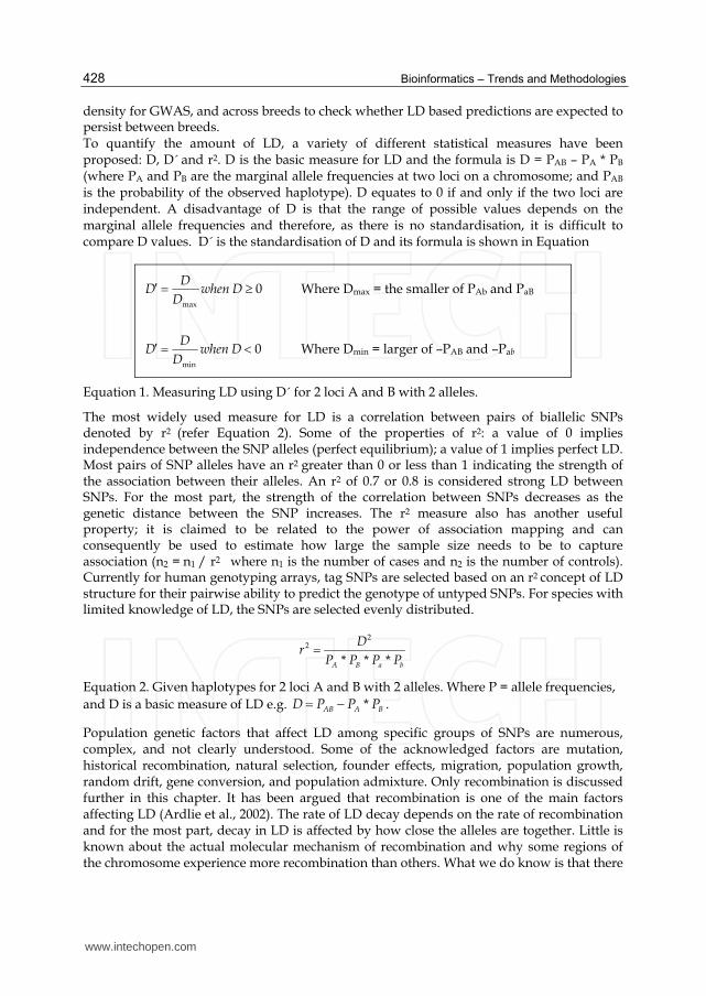
density for GWAS, and across breeds to check whether LD based predictions are expected to persist between breeds. To quantify the amount of LD, a variety of different statistical measures have been proposed: D, D´ and r2. D is the basic measure for LD and the formula is D = PAB – PA * PB (where PA and PB are the marginal allele frequencies at two loci on a chromosome; and PAB is the probability of the observed haplotype). D equates to 0 if and only if the two loci are independent. A disadvantage of D is that the range of possible values depends on the marginal allele frequencies and therefore, as there is no standardisation, it is difficult to compare D values. D´ is the standardisation of D and its formula is shown in Equation

max

0D

D when DD

Where Dmax = the smaller of PAb and PaB

min

0D

D when DD

Where Dmin = larger of –PAB and –Pab

Equation 1. Measuring LD using D´ for 2 loci A and B with 2 alleles.

The most widely used measure for LD is a correlation between pairs of biallelic SNPs denoted by r2 (refer Equation 2). Some of the properties of r2: a value of 0 implies independence between the SNP alleles (perfect equilibrium); a value of 1 implies perfect LD. Most pairs of SNP alleles have an r2 greater than 0 or less than 1 indicating the strength of the association between their alleles. An r2 of 0.7 or 0.8 is considered strong LD between SNPs. For the most part, the strength of the correlation between SNPs decreases as the genetic distance between the SNP increases. The r2 measure also has another useful property; it is claimed to be related to the power of association mapping and can consequently be used to estimate how large the sample size needs to be to capture association (n2 = n1 / r2 where n1 is the number of cases and n2 is the number of controls). Currently for human genotyping arrays, tag SNPs are selected based on an r2 concept of LD structure for their pairwise ability to predict the genotype of untyped SNPs. For species with limited knowledge of LD, the SNPs are selected evenly distributed.

22

* * *A B a b

Dr

P P P P

Equation 2. Given haplotypes for 2 loci A and B with 2 alleles. Where P = allele frequencies,

and D is a basic measure of LD e.g. *AB A BD P P P .

Population genetic factors that affect LD among specific groups of SNPs are numerous, complex, and not clearly understood. Some of the acknowledged factors are mutation, historical recombination, natural selection, founder effects, migration, population growth, random drift, gene conversion, and population admixture. Only recombination is discussed further in this chapter. It has been argued that recombination is one of the main factors affecting LD (Ardlie et al., 2002). The rate of LD decay depends on the rate of recombination and for the most part, decay in LD is affected by how close the alleles are together. Little is known about the actual molecular mechanism of recombination and why some regions of the chromosome experience more recombination than others. What we do know is that there

www.intechopen.com


is variation in recombination rates, and regions of recombination appear and disappear over evolutionary time. By studying the patterns of LD we can at least infer the distribution of recombination events. In the literature LD is intertwined with the term haplotype. There are many definitions of the term haplotype in the literature, herein haplotype is used as being half of a genotype, that is, a set of ordered SNP alleles on a single chromosome that are transmitted as one unit from a parent to an offspring (Ardlie et al., 2002). Theoretically a haplotype, one unit, could comprise any number of SNPs from only 2 SNPs to every single SNP on the chromosome. In reality, however, recombination events result in haplotype blocks comprised of varying numbers of SNPs. Early studies of pairwise LD (i.e. using 2-locus haplotypes) observed complex patterns of LD implying a random nature. It is now becoming clear that despite many generations of segregation from a common ancestral chromosome, certain combinations of neighbouring SNP alleles (haplotype units) have remained unchanged. In other words, there are stretches of DNA that are almost never divided during meiosis (Gibbs et al., 2003). Although we do not fully understand the biological processes that give rise to recombination in some regions of the chromosome and not in others, there still appears to be some non-random underpinning mechanism. More recently the International Hapmap Project (Gibbs et al., 2003) has shown that the underlying structure of LD in a genome could be divided into discrete haplotype blocks. Using evidence from their LD measures, a haplotype block represents a region with a few haplotypes (2-4 per block) in a population separated by a region with many haplotypes in the population. Their proposed haplotype block model of LD, from a recombination perspective, is a region of high LD separated by recombination hotspots. There are two popular methods for block definition: 1) using pair-wise disequilibrium to define regions of high LD separated by recombination hotspots, and 2) defining regions with high or low haplotype diversity.

1.2 Phasing SNP genotypes for deriving paternal and maternal haplotypes

We currently have the technology to observe genotypes but not haplotypes. That is, we do not observe individual alleles on the chromosome. This immediately presents a problem for haplotype analysis since the phase is not known when SNPs are heterozygous. For example, given the genotype of 2 SNPs with homozygous alleles at 2 different loci, “11” and “22” respectively; the haplotype on both the paternal and maternal chromosome is conclusively “12”. However, given the genotype of 2 SNPs with heterozygous alleles, “12” and “12”; we do not know which allele is inherited from which parent. The possible haplotypes are shown in Figure 1. We cannot say for certain which alleles on a haplotype go together when using genotype data with heterozygous SNP alleles. Consequently we need to determine or infer the phase from other methods. There are 3 possible methods available to the researcher: 1) use pedigree information; 2) use molecular methods to single out individual chromosomes to do genotyping (currently only possible on small regions; and 3) statistical methods to infer the haplotype given genotype data. From literature, there are several algorithms and programs for inferring haplotypes. Two of the most popular programs are called PHASE, which uses algorithms based on Bayesian coalescent models Stephens et al. (2001) and fastPHASE, which uses an EM algorithm and cluster model Scheet et al. (2006). The default PHASE and fastPHASE output format has been adopted as the format required for the input data to SNPpattern.

www.intechopen.com


Fig. 1. Possible haplotype when 2 SNPs have heterozygous alleles.

PHASE is a statistical method inspired from coalescent theory. The coalescent theory in essence is the tracing of alleles, shared in a sample of individuals from a population, back to the most recent common ancestor Fu et al. (1999). This theory can predict the expected patterns of haplotypes in natural populations. The PHASE method is Bayesian and uses the a priori expectation of haplotypes to inform haplotype reconstruction (see Equation 3). The phase reconstruction procedure is to evaluate the conditional distribution of the unknown haplotypes corresponding to the genotypes for the individuals from a population sample. PHASE uses Gibbs sampling (Kim, 2001) to obtain an approximate sample from the posterior distribution of unknown haplotype pairs given genotype data (e.g. Pr (H | G) is the posterior probability that the reconstruction of the haplotype pairs is correct, given the genotypes and knowledge of previous haplotype reconstruction states). In the most simplistic terms, the algorithm begins by estimating the haplotypes for a randomly chosen individual on the assumption all other haplotypes are reconstructed correctly. The algorithm reiterates the process enough times to result in an approximate haplotype reconstruction from the posterior probability. Stephens[38] claims that PHASE, “is sufficiently accurate that reconstructing haplotypes experimentally, or by genotyping additional family members, may be an inefficient use of resources”.

Pr( | ) Pr( )Pr |

Pr( )

G H HH G

G

Equation 3. Bayes theorem.

where, Pr(H|G) is the conditional probability that the reconstruction of the haplotype pairs is correct given the genotypes. Pr(H) is the prior (unconditional) probability the reconstruction of the haplotype pairs is correct irrespective of genotype data. P(G) is the total probability of observed genotypes across all possible haplotypes (acts as a normalising constant).

Where P = chromosome inherited from father; M = chromosome inherited from mother; Genotype for SNPs = 12)

www.intechopen.com


Pr(G|H) is the conditional probability of obtaining the genotypes given the haplotypes. The fastPHASE software package is a statistical model that captures patterns of LD. The variation in the patterns can be applied to estimate missing genotypes and to infer haplotype phase in samples of unrelated individuals from natural populations from unphased genotype data. The fastPHASE statistical model uses an “approximate coalescent with recombination” prior manifested from the fact that over short genomic regions haplotypes in a population have been observed to cluster into groups of similar haplotypes because of recombination (Stephens et al., 2005). The model also considers each cluster of observed haplotypes to represent a common haplotype and each haplotype is assumed to have evolved from a single cluster. The membership of each cluster is allowed to change along the chromosome in accordance with a hidden Markov model (Scheet et al., 2006). An expectation-maximization (EM) algorithm (Dempster et al., 1997) is used to estimate the model parameters. The paper presents the development of SNPpattern as a simple bioinformatic tool to rapidly screen the genome for haplotype structure, perform some basic descriptive genome statistics and link interesting haplotypes to functional information. We have tested our software SNP pattern on Ovine 60k SNPchip data (Goodswen et al., 2010). One impetus for the development of SNPpattern was to understand the degree of diversity in LD architecture between different livestock breeds (McKay et al. 2007). It was thought that with our increased understanding we could potentially predict effect of genome selection across breeds, which is based on SNPs being in LD with causal variants for the trait of interest. In addition, we expect SNPpattern be used in the comparison of LD structure in detecting and localizing genomic regions where selective sweeps2 have occurred (Smith et al., 1974).

2. Development of SNPpattern

A commonly used software package for computing LD statistics and haplotype patterns for populations from genotype data is Haploview (Barrett et al., 2005). One of the interesting features of Haploview, is its ability to generate haplotype blocks. Haploview has a number of methods to partition the genome into blocks: 1) block definitions are based on D' confidence bounds e.g. SNP pairs are defined to be either “strong LD” (.i.e. no evidence of historical recombination) or “strong recombination”. The algorithm is taken from Gabriel et al. (2002); 2) the block definition is based on a four gamete test of Hudson & Kaplan (1985) proposed by Wang et al (2002). In brief, for each SNP pair, the population frequencies of the 4 possible two-SNP haplotypes are computed (e.g. SNP 1 = A/a and SNP 2 = B/b. The 4 haplotypes are AB, Ab, aB, and ab). If all 4 haplotypes are observed with a frequency >= 0.01 (a user definable threshold), a recombination is assumed to have occurred. If only 3 haplotypes are observed no recombination is assumed. A block is formed when there has been no recombination for successive SNP pairs. HaploBlock is a software package, which has as one of its capabilities the inference of haplotype block models from phased or unphased data. It primarily uses a Markov chain and can account for recombination hotspots, bottlenecks, genetic drift and mutations (Greenspan & Geiger, 2004). HapBlock (a different program to the similarly named

2 A selective sweep can be caused when there is a strong directional selection for a favourable new allele

that increases its frequency. Alleles in close proximity to the new allele are “swept” to fixation.

www.intechopen.com


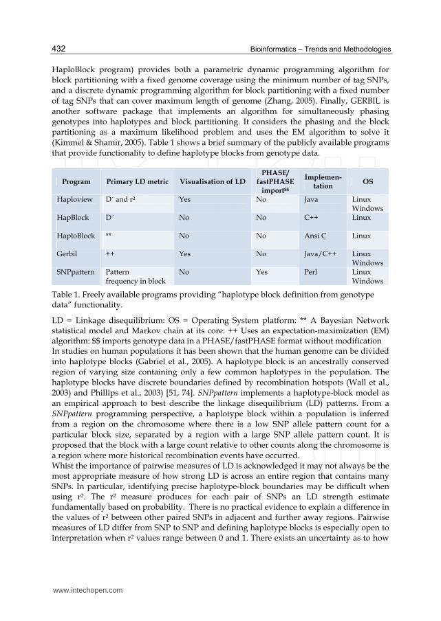
HaploBlock program) provides both a parametric dynamic programming algorithm for block partitioning with a fixed genome coverage using the minimum number of tag SNPs, and a discrete dynamic programming algorithm for block partitioning with a fixed number of tag SNPs that can cover maximum length of genome (Zhang, 2005). Finally, GERBIL is another software package that implements an algorithm for simultaneously phasing genotypes into haplotypes and block partitioning. It considers the phasing and the block partitioning as a maximum likelihood problem and uses the EM algorithm to solve it (Kimmel & Shamir, 2005). Table 1 shows a brief summary of the publicly available programs that provide functionality to define haplotype blocks from genotype data.

Program Primary LD metric Visualisation of LD PHASE/

fastPHASE import$$

Implemen- tation

OS

Haploview D´ and r2 Yes No Java Linux Windows

HapBlock

D´ No No C++ Linux

HaploBlock

** No No Ansi C Linux

Gerbil ++ Yes No Java/C++ Linux Windows

SNPpattern Pattern frequency in block

No Yes Perl Linux Windows

Table 1. Freely available programs providing “haplotype block definition from genotype data” functionality.

LD = Linkage disequilibrium: OS = Operating System platform: ** A Bayesian Network statistical model and Markov chain at its core: ++ Uses an expectation-maximization (EM) algorithm: $$ imports genotype data in a PHASE/fastPHASE format without modification In studies on human populations it has been shown that the human genome can be divided into haplotype blocks (Gabriel et al., 2005). A haplotype block is an ancestrally conserved region of varying size containing only a few common haplotypes in the population. The haplotype blocks have discrete boundaries defined by recombination hotspots (Wall et al., 2003) and Phillips et al., 2003) [51, 74]. SNPpattern implements a haplotype-block model as an empirical approach to best describe the linkage disequilibrium (LD) patterns. From a SNPpattern programming perspective, a haplotype block within a population is inferred from a region on the chromosome where there is a low SNP allele pattern count for a particular block size, separated by a region with a large SNP allele pattern count. It is proposed that the block with a large count relative to other counts along the chromosome is a region where more historical recombination events have occurred. Whist the importance of pairwise measures of LD is acknowledged it may not always be the most appropriate measure of how strong LD is across an entire region that contains many SNPs. In particular, identifying precise haplotype-block boundaries may be difficult when using r2. The r2 measure produces for each pair of SNPs an LD strength estimate fundamentally based on probability. There is no practical evidence to explain a difference in the values of r2 between other paired SNPs in adjacent and further away regions. Pairwise measures of LD differ from SNP to SNP and defining haplotype blocks is especially open to interpretation when r2 values range between 0 and 1. There exists an uncertainty as to how

www.intechopen.com


one LD estimate in one region relates to an LD estimate in another region because SNP pairs are not necessarily independent (i.e. one region may functionally affect another region) and consequently this diminishes the certainty of which SNPs belong to which haplotype block. For example, there are cases where 2 SNPs exhibit strong pairwise LD but show different r2 to a SNP in between, and a low strength pairwise LD is not necessarily indicative of high ancestral recombination. In other words, SNPs in close proximity are not always in pairwise LD and by contrast, SNPs far apart can be in pairwise LD (Phillips et al., 2003). We can also expect the haplotype block boundaries to be different depending on the sample size and SNP density used. Another limitation of r2, particularly for marker-assisted selection in livestock, is that the r2 can be the same between a SNP marker and a potential causal variant in different populations, and yet the phase may be different (Roos et al., 2008). Deriving clear information about the joint inheritance of alleles in a chromosome segment is also expected not to be easy from r2 measures. It is argued instead that we can infer the joint inheritance of alleles from inferring which haplotype blocks were inherited, if we know which haplotype blocks exist in a particular population i.e. we can make inference about identity by descent (IBD) of alleles in particular regions. In light of some of these shortcomings discussed, a multiple SNP allele block approach in preference to r2 was implemented through SNPpattern. The required input data for SNPpattern is phased genotype data from either a single group or multiple groups of individuals (e.g. from different animal breeds or subpopulations). The premise for the multiple SNP allele block approach is to count the frequency of SNP allele blocks, of different sizes, found in the genomes of the group members. For example, a block of 5 SNPs spanning a few thousand base pairs could potentially comprise 32 different SNP allele patterns if the SNPs were totally independent and the population was of infinite size (the number of possible SNP allele patterns is 2n where n is the number of SNPs in the block). The general process of the program is that it counts the frequency of the various SNP allele patterns found in the same chromosomal location (the same SNP allele block region) across each individual in the group sample; then repeats the process for the next SNP allele block region along the genome, and so on. From the counts we can infer the haplotype blocks after taking into account the population structure and allelic frequencies (a user of SNPpattern also needs to be aware that there are numerous other population genetic factors that affect LD and determine haplotypes). The inferred haplotype block represents a region with a few distinct SNP allele patterns (indicating small amount of haplotype variation) in a population separated by a region with many SNP allele patterns (indicating an excessive amount of haplotype variation) in the population. In a typical short chromosome segment, we can expect only a few distinct SNP allele patterns. Hence the larger the SNP allele block size the less likely the distinct SNP allele patterns appear by chance because of the increased probability of recombination over larger distances. It is argued that the comparison of SNP allele pattern counts can be used as a measure of genetic distance and this comparison forms the basis for a haplotype diversity analysis within and between groups. In addition to implementing the core components for the multiple SNP allele block approach, SNPpattern also implements similarity scoring between individuals. We can expect that the more the SNP allele patterns between two individuals are similar the more likely they will have a similar haplotype structure. Taking this one step further, if two individuals share the same extended SNP allele patterns over the same genomic region, the chance that they carry the same causal variant allele relationship by descent is much higher.

www.intechopen.com


Linkage disequilibrium mapping to identify the chromosomal region (the haplotype block) containing a QTL has proven to be a powerful tool Barrett et al., (2005) and Hayes et al., (2006). However, once the haplotype block has been identified, LD provides no further information to help localize the actual variants within the block (Rioux, 2001). It has been proposed that advantageous mutations through directional selection are more likely to occur in a region of low recombination (Wall et al., 2003). Conversely, there is evidence that there are alleles in recombination hotspots that are more likely to initiate the double-strand break associated with recombination (Jeffreys & Neumann, 2002). One of the outputs from SNPpattern is a list of chromosomal start and end locations of SNP allele blocks identified to have low and/or high haplotype diversity. In the program testing section of this chapter, how this output list could be used to link these identified regions to genomic annotation is demonstrated. We used the FunctSNP R package that we have developed earlier (Goodswen et al., 2010) .To recover the biology role of genomic regions with low haplotype diversity, a systems genetics or system biology approaches would be needed, as demonstrated in Kadarmideen et al., (2006) and Kadarmideen (2008).

3. Implementation of SNPpattern

SNPpattern was written in the Perl programming language. The following sections describe the methods and rationale that have shaped the development. We have tested SNP pattern on Ovine 60k SNPchip data and these results are based on our earlier work (Goodswen et al., 2010).

3.1 Input data

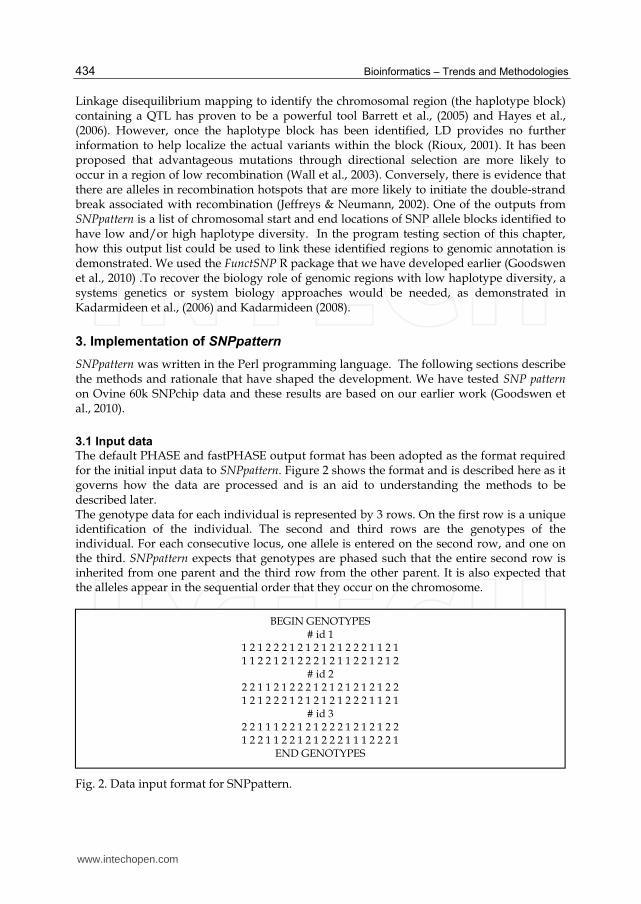
The default PHASE and fastPHASE output format has been adopted as the format required for the initial input data to SNPpattern. Figure 2 shows the format and is described here as it governs how the data are processed and is an aid to understanding the methods to be described later. The genotype data for each individual is represented by 3 rows. On the first row is a unique identification of the individual. The second and third rows are the genotypes of the individual. For each consecutive locus, one allele is entered on the second row, and one on the third. SNPpattern expects that genotypes are phased such that the entire second row is inherited from one parent and the third row from the other parent. It is also expected that the alleles appear in the sequential order that they occur on the chromosome.

Fig. 2. Data input format for SNPpattern.

BEGIN GENOTYPES # id 1

1 2 1 2 2 2 1 2 1 2 1 2 1 2 2 2 1 1 2 1 1 1 2 2 1 2 1 2 2 2 1 2 1 1 2 2 1 2 1 2

# id 2 2 2 1 1 2 1 2 2 2 1 2 1 2 1 2 1 2 1 2 2 1 2 1 2 2 2 1 2 1 2 1 2 1 2 2 2 1 1 2 1

# id 3 2 2 1 1 1 2 2 1 2 1 2 2 2 1 2 1 2 1 2 2 1 2 2 1 1 2 2 1 2 1 2 2 2 1 1 1 2 2 2 1

END GENOTYPES

www.intechopen.com


3.2 Grouping data In its simplest form, SNPpattern will accept an input, such as the one shown in Figure 2, and treat all individuals as members of the same group. The output will consequently be results for haplotype diversity within a group. The results will also be for the entire genome without any reference to the chromosomal location of the haplotypes. In spite of this, it is expected (although not mandatory) that an additional file be provided as input, which contains phenotypic information about the individual. Table 2 shows as an example the first 9 lines of a fictitious phenotype file and in this instance one specific to livestock species. Grouping data is obviously an essential part of the evaluation of haplotype diversity between groups. It is also a hugely critical part to account for the count biases that may be introduced due to population structure. For example, if in a particular sire breed group the number of progeny from each sire is disproportionate then the SNP allele pattern count will be biased in favour of the progeny with the largest number of siblings. Grouping an equal number of progeny from each sire should prevent the bias. SNPpattern includes the functionality to group the genotype data of individuals according to user-defined criteria specific to information held in columns in a phenotypic file. Theoretically the program can create a group based on any combination of columns when using the “AND” Boolean logic. For example, group all individuals according to sire breed AND year of birth. Separate output files for each group criteria are generated containing the genotype data of the group members. The output format is the same as that shown in Figure 2. The program also allows the user to use comparison operators (=, >=, <=, >, <) on any combination of column criteria. For example, if we want to group all the female progeny in area 03 born after the year 1972 having a particular parent ID, the equivalent pseudo code is sex = F AND Area = 03 AND Year of Birth > 1975 AND parent ID = 433. The grouping of the data is of course at the discretion of the researcher to create genetically meaningful groups. Summary information about the groups can also be generated. SNPpattern provides the flexibility of the grouping through a configuration file in an INI file format. Another optional file that can be provided as input is a SNP mapping file. Such a file allows the contents of a group file to be divided further into separate chromosome files. This division of the genotypes for the entire genome into their respective chromosome locations allows for the comparison of haplotype diversity of a particular chromosome in one group with the same chromosome number in another group. The fact that selective sweeps act differently in different chromosomes is one example as to why a study of haplotype diversity may be needed on a chromosome basis (Montpetit & Chagnon, 2006). It is mandatory that the SNP mapping file contains the SNP location and the chromosome number on which it resides. SNPpattern expects the SNPs in the file to be in the order that they are located on the chromosome. It is also an expectation that the SNP mapping file is most likely obtained from another source and will contain redundant information to SNPpattern. Therefore another configuration file, specific to dividing the genome into chromosomes, allows extraction of only the required SNP location and the chromosome number without the need for the researcher to modify the SNP mapping file. It may be arguable as to why a separate file is created for each group and/or each chromosome sub-group. From a programming perspective separate files are created for 3 reasons: 1) the output file format used is the same as PHASE and fastPHASE. It is envisaged that the SNPpattern group files could be imported into other programs that use this same format; 2) the separate files are a permanent record of the grouping that can be reused, as opposed to temporary grouping only at runtime; and 3) the data files can be extremely large and slower to parse the content if all groups are recorded separately but in the one file.

www.intechopen.com


Human ID Parent ID Region Sex Parent ethnicity Year of birth Body Weight (kg)

1 330 01 F American 1978 74.6 2 330 01 M American 1971 99.0 3 405 02 F African 1970 77.4 4 405 02 M African 1975 63.6 5 433 03 M Asian 1972 79.0 6 433 03 M Asian 1971 67.0 7 433 04 F Asian 1979 73.0 8 405 05 F European 1974 97.4 9 405 05 M European 1976 94.0

Table 2. Example contents of a phenotypic file.

3.3 Multiple SNP allele block approach

This section describes the multiple SNP allele block approach implemented through SNPpattern. We have tested SNP pattern on Ovine 60k SNPchip data and tables 3-6 are based on our already published work (Goodswen et al., 2010). With reference to Figure 2 the 2 rows of biallelic SNPs contained within the phased genotype file are extracted (in this instance, a single 1 or 2 constitutes a SNP allele). One row represents the SNP alleles inherited from one parent, and the second row represents the SNP alleles inherited from the other parent. So in effect, we have a representation of paternal and maternal chromosomes composed of a long serial SNP allele pattern of 1s and 2s. Without prior knowledge, the user will not know which row represents which parental chromosome. However, when the SNP allele pattern analysis progresses the identity of the row representation may become apparent as will be demonstrated in the program testing section. The underlying unit of the multiple SNP allele block approach is of course the SNP allele block. The serial SNP allele pattern from one row (e.g. representing the chromosome inherited from the paternal side) is divided into block sizes of any specified number of SNP alleles at the discretion of the researcher e.g. 3, 5, 10 or 100 (or larger) SNP alleles per block. Then if required, the SNP allele pattern from the other row is divided into blocks of the same specified size. Figure 3 shows the first 40 numbers of a SNP allele pattern of 1s and 2s that represents either a paternal or maternal chromosome for one individual. In this example, the entire SNP allele pattern is divided into blocks of 3 e.g. the first 3 blocks are “112”, “212”, and “211”. For a n SNP allele block there are 2n possible SNP allele pattern combinations of 1 and 2. Therefore, a 3 SNP allele block has 23 possible patterns (111, 112, 121, 122, 211, 212, 221, and 222). For each SNP allele block along the row that represents either the paternal or maternal chromosome, we count how many individuals in the group have the same SNP allele pattern. For example, at block location 1 (Figure 3) we count, for each of the 8 possible SNP allele combinations, how many individuals have the SNP allele pattern “111”, then “112” etc. Table 3 shows an example of the SNP allele pattern count at the first 3-SNP allele block along a paternal chromosome. We could expect an equal chance of observing any one of the 8 possible SNP allele combinations (assuming the SNP allele frequencies were equal) if there was no underlying association between the 3 SNPs in the block. In reality however, we have a SNP allele pattern count profile which is a result of many generations of random and non-random SNP inheritance from a common ancestor. A challenge is to determine which of the 8 possible SNP allele combinations exist because the 3 SNPs were inherited by descent from a common ancestor and which SNP allele combinations exist by chance alone. For long SNP

www.intechopen.com


Fig. 3. Consecutive 3-SNP allele blocks along 1 row representing either a paternal or maternal chromosome.

allele patterns (e.g. 10 or more SNP alleles per block)3 that can be inferred to be a haplotype block, identity is more likely by descent. For short SNP allele patterns (e.g. 3 SNP alleles per block) inferred to be a haplotype block, it is more likely identical by chance. Nevertheless, we can statistically test whether the observed count distribution has arisen from independently segregating SNPs. On the other hand, it is debatable whether the test will achieve the desired results. If SNPs are very close then we would expect SNPs not to segregate independently, and the observed counts arise more from genetic drift (i.e. some SNP allele patterns are more frequent due to limited population size and the large effect of the contribution of only some ancestors to the current population). Despite the latter concern, in an attempt to meet this challenge, expected and observed counts are still tested for statistical significance. To determine the expected SNP allele pattern count, SNPpattern computes the SNP allele frequencies (Table 3). For example, the expected proportion for SNP allele pattern “111” based on the allelic frequencies of each of the 3 SNPs and assuming independence is 0.072 ( Pr(SNP 1 allele 1) * Pr(SNP 2 allele 1) * Pr(SNP 3 allele 1)). The expected count for SNP allele pattern “111” is therefore 72 (proportion expected * number of individuals). Based on the allele frequencies, the null hypothesis is that we expect the observed and expected count to be the same, and as a consequence the SNPs to be independent (i.e. SNPs are segregating independently). A Fisher's Exact Test4 for count data is applied as a statistical significance test for each SNP allele pattern. Table 5 shows an example of how the data for SNP allele pattern “111” from Table 4 is used in a 2 * 2 contingency table to compute the exact probability of observing a table with this result (Equation 4). The p-values are obtained directly using the hypergeometric distribution. The p-values (examples shown in Table 3) are used as the conditional criteria to determine which SNP allele patterns were most likely to have occurred by chance. In this example, the low p-value for pattern “111” indicates that the hypothesis is unlikely to be true and therefore the SNPs within the pattern are not independent. The success as to whether the challenge was met of distinguishing SNPs in a haplotype block from SNPs in a random pattern is reviewed in the discussion section. From a SNPpattern implementation perspective, some difficulty was encountered in programming Fisher's Exact Test. A Perl module (Text::NSP::Measures::2D::Fisher2) downloaded from CPAN5 is currently being investigated for its suitability. As an interim

3 Dependent on the chromosomal distance between SNPs 4 Used in preference to Chi-Square test since expected counts may be less than 5 5 The Comprehensive Perl Archive Network

1122122111111112112112112221212122111222 … continued

1 2 3 4 5 SNP allele blocks

www.intechopen.com


SNP allele pattern

Observed SNP allele pattern

count

Expected SNP allele pattern

count

Proportion Observed

Proportion expected

p-value$$

111 14 72 0.014 0.072 6.07e-11 112 32 27 0.032 0.027 0.598 121 699 652 0.697 0.650 0.097 122 241 242 0.240 0.241 1.000 211 0 1 0 0.001 - 212 0 0 0 0.000 - 221 17 7 0.017 0.007 0.062 222 0 2 0 0.002 -

Total 1003++ 1003++ 1.000 1.000

++ Number of individuals in group $$ p-values are obtained directly using the hypergeometric distribution following a Fisher's Exact Test

Table 3. Example of SNP allele pattern counts at the first 3-SNP allele block along a paternal chromosome based on Goodswen et al., (2010)

measure, the statistical programming language R (http://www.r-project.org/) was used. SNPpattern can output a file containing a list of the observed SNP allele pattern counts per block in the first column and the expected SNP allele pattern counts per block (computed from the individual SNP allele frequencies) in the second column. The output file can be read directly into R and used as input to the function fisher.test () to conduct the Fisher's Exact Test for count data.

SNP 1 SNP 2 SNP 3 Count Count Count

Allele Row 2++ Row 3 Freq.$$ Row 2 Row 3 Freq. Row 2 Row 3 Freq.

1 986 993 0.99 46 161 0.10 730 733 0.73 2 17 10 0.01 957 842 0.90 273 270 0.27

Total 1003 1003 1.00 1003 1003 1.00 1003 1003 1.00

++ Row 2 and Row 3 are the rows that represent the genotype data for each individual (refer Figure 4-1). For genotype at SNP #1, 986 out of a total of 1003 individuals have a ‘1’ on row 2, and 17 out of 1003 have a ‘2’ a row 2 $$ Freq. = Allelic Frequency. For example, the population frequency of ‘1’ at the SNP 1 location is (986 + 993) /2006 = 0.99. Likewise the population frequency of ‘2’ at the SNP 1 location is (17 + 10)/ 2006 = 0.01

Table 4. Example of allele frequencies for 3 sequential SNPs.

Observed Expected Row totals

Pattern found 14a 72b 86a+b

Pattern not found 989c 931d 1920c+d

Column totals 1003a+c 1003b+d 2006n

Table 5. A 2 * 2 contingency table for SNP allele pattern "111".

( ) !( )!( )!( )!Pr( , , , )

! ! ! ! !

a b c d a c b da b c d

n a b c d

Equation 4. Fisher’s formula for exact probability of observing the data in a contingency table.

www.intechopen.com


Table 4 shows the SNP allele pattern count for the first 6 consecutive blocks for a 10-SNP allele block size for a paternal chromosome. From the counts we can infer haplotype blocks. As per the SNPpattern premise for a haplotype block previously described in the introduction, it is a region with a low SNP allele pattern count separated by a region with a large SNP allele pattern count. In other words, it is expected that if a block has a large SNP allele pattern count relative to the counts within other blocks along the chromosome, it is likely to be a recombination hotspot. For each paternal or maternal chromosome, SNPpattern computes descriptive statistics such as the average number and standard deviation of patterns found per block. A user definable count threshold can be applied to filter large SNP allele patterns counts to infer the haplotype blocks. By default SNPpattern flags SNP allele patterns with counts greater than 1 standard deviation above average. Of course, the relevant count threshold to use and the interpretation of inferred haplotype blocks requires thorough knowledge of group population structure. It is therefore critically important that judicious grouping of genotypes takes place prior to the SNP allele pattern counts (refer previous section – Grouping data). Another point to note is that the chromosomal distance between SNPs is not equal and therefore the physical size of the each block of SNPs is not equal. Although SNPpattern computes and reports the physical block sizes, it does not adjust the SNP allele pattern counts to compensate for unequal sizes.

SNP ALLELE BLOCKS

1 2 3 4 5 6

Pattern count 70 69 115 76 57 20

H/L flag ++ L L H L L L

Physical block size 619948 520686 437805 394152 398511 538789

++ H indicates block with SNP allele pattern count greater than user defined threshold; L indicates block with SNP allele pattern count less than threshold

Table 6. SNP allele pattern counts per 10-SNP allele block along paternal chromosome.

In summary, for this section on the multiple SNP allele block approach, using SNP allele pattern frequency counts as a measure, we can make comparisons between individuals, groups of individuals, and groups. These comparisons then allow us to make informed decisions about the general haplotype diversity. It is also expected that processing the same genotype data several times using different block sizes, we can fine-tune the distribution of the haplotype blocks. Finding similarity between individuals. The method presented in this section was inspired from publications [80-83] on genetic distance and similarity matrices. Two genetically identical individuals (i.e. identical DNA sequences throughout the genome) will have identical haplotype structures. It therefore could be argued that the more genetically similar two individuals are to each other, the more likely they will have the same haplotype structure. In other words, the closer two individuals are related the more the DNA sequences are expected to be in common. The genotyped SNPs are of course not as accurate a unit of comparison as genome wide nucleotide sequences. However, it is not unreasonable to assume that comparing the SNP allele patterns between two individuals will provide a guideline as to the similarity of haplotype structure. So, although this method does not show the actual haplotype structure, the overall similarity in SNP allele patterns between individuals or groups of individuals will give an indication of similarity in haplotype structure. As a simple example we take 3

www.intechopen.com


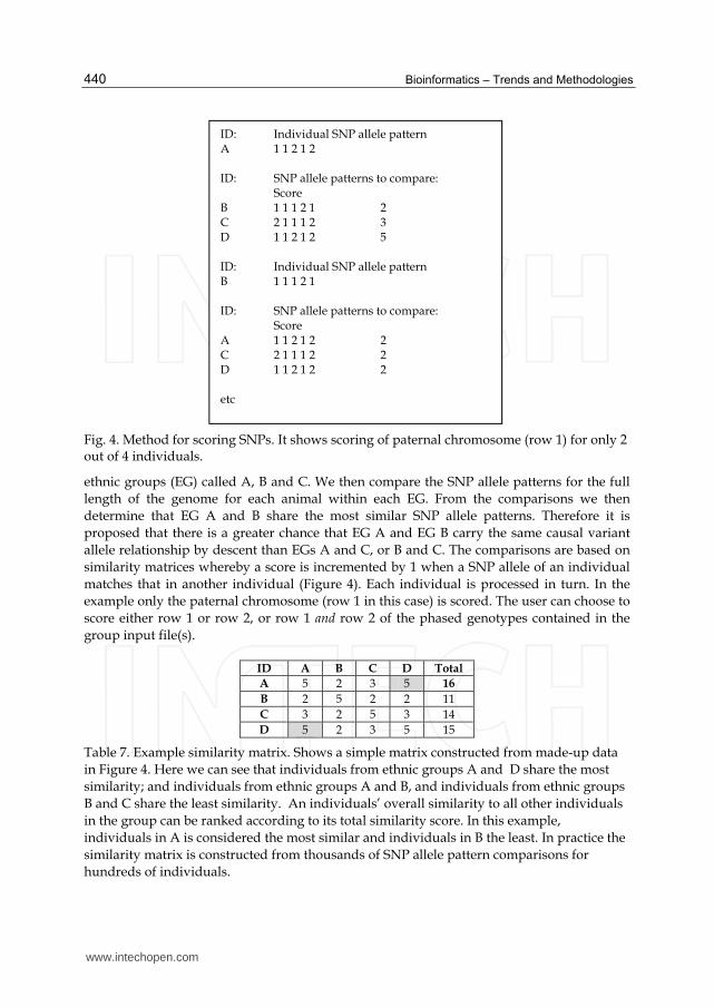
Fig. 4. Method for scoring SNPs. It shows scoring of paternal chromosome (row 1) for only 2 out of 4 individuals.

ethnic groups (EG) called A, B and C. We then compare the SNP allele patterns for the full length of the genome for each animal within each EG. From the comparisons we then determine that EG A and B share the most similar SNP allele patterns. Therefore it is proposed that there is a greater chance that EG A and EG B carry the same causal variant allele relationship by descent than EGs A and C, or B and C. The comparisons are based on similarity matrices whereby a score is incremented by 1 when a SNP allele of an individual matches that in another individual (Figure 4). Each individual is processed in turn. In the example only the paternal chromosome (row 1 in this case) is scored. The user can choose to score either row 1 or row 2, or row 1 and row 2 of the phased genotypes contained in the group input file(s).

ID A B C D Total

A 5 2 3 5 16

B 2 5 2 2 11

C 3 2 5 3 14

D 5 2 3 5 15

Table 7. Example similarity matrix. Shows a simple matrix constructed from made-up data in Figure 4. Here we can see that individuals from ethnic groups A and D share the most similarity; and individuals from ethnic groups A and B, and individuals from ethnic groups B and C share the least similarity. An individuals’ overall similarity to all other individuals in the group can be ranked according to its total similarity score. In this example, individuals in A is considered the most similar and individuals in B the least. In practice the similarity matrix is constructed from thousands of SNP allele pattern comparisons for hundreds of individuals.

ID: Individual SNP allele pattern A 1 1 2 1 2 ID: SNP allele patterns to compare: Score B 1 1 1 2 1 2 C 2 1 1 1 2 3 D 1 1 2 1 2 5 ID: Individual SNP allele pattern B 1 1 1 2 1 ID: SNP allele patterns to compare: Score A 1 1 2 1 2 2 C 2 1 1 1 2 2 D 1 1 2 1 2 2 etc

www.intechopen.com


3.4 Linking SNP allele block regions to genomic annotation

One of the output files from a SNPpattern Perl script is a file that contains all SNP allele

blocks where the number of distinct SNP allele patterns is low or high. The script allows

for a user-definable upper or lower pattern frequency threshold. For example, if a user

enters a threshold of “<3” then only SNP allele blocks with a distinct SNP allele pattern

frequency of less than 3 will be output. Likewise, if the user enters “>99” only SNP allele

blocks with a distinct SNP allele pattern frequency of greater than 99 will be output.

Figure 4-4 shows an example of the output file. The output consists of a list with 4

columns: Chromosome number of the chromosome containing the SNP allele block (the

genomic region of interest); start and end genomic location of SNP allele block; the

number of distinct SNP allele patterns found within the SNP allele block for a group of

individuals (only lists the genomic regions where the number of patterns is below or

above a user-defined threshold), and the average number of patterns per block. The

intended use of the output file is to act as a starting point for a researcher to find

biological meaning in regions identified to have low or high haplotype diversity.

Biological meaning may help in the understanding of why in some regions and not others

there is a conservation of the same alleles from generation to generation. In other words,

why is there only 1 or 2 distinct SNP allele patterns existing in the same genomic region

for all individuals in a group? Conversely, some regions have a large number of different

SNP allele patterns implying a hotspot region for recombination. Finding the underlying

biology within the hotspot region may provide clues to the mechanism of recombination.

The expectation is that the output list can be used for further downstream analysis such as

searching for annotation of the chromosome region within which the SNP allele block is

located.

Fig. 5. Example output file showing genomic regions with low SNP allele pattern counts.

As an example, we could find the genes within the genomic region. In the FunctSNP R

package (5) there is a function called “getGenesByRange” which returns the Gene ID for all

genes located between a user-specified start and end location.

3.5 Implementation summary

In summary, three sets of Perl scripts comprise SNPpattern: 1) grouping data scripts – to

create separate data files for further downstream comparison analysis; 2) SNP allele block

scripts – to find, count, and compare the SNP allele block patterns between any group of

individuals; and 3) similarity scripts - to score the similarity between individuals based on

an individual’s entire SNP allele pattern. Table 8 encapsulates the primary function and

rationale of each script.

# Input file used: sire_31_match_10.txt # Pattern Size: 10 # Haplotype row: paternal # Chromosome No: Start of pattern: End of pattern: No. of Patterns: Average No. per block 4 3000848 3170609 2 6.58 13 67400889 67687804 2 4.09

www.intechopen.com


Perl Script Name (.pl)

Primary function Rationale

Scripts for grouping and summarising genotype data

Group Genotype data is separated into files according to a grouping criterion. For example, the genotype of animals can be grouped according to their sire breed, or flock ID, or birth years.

Main purpose of dividing the data into groups is to account for population structure, facilitate the SNP-block pattern counting within a group and the comparison of the SNP-block pattern count between groups.

divide Divide the bi-allelic SNPs in any group input file (e.g. flock, breed, and sire groups) into separate chromosome files.

Used as the main input for the SNP allele pattern analysis scripts and in particular for the multiple SNP allele block approach

Scripts for finding, counting, and comparing SNP allele block patterns

derive_pattern Derive all SNP allele patterns of a specified block size (e.g. 3, 100, 1000, 2000 etc.) that exist in the maternal and/or paternal chromosomes for any group file (e.g. either flock, breed, or sire)

Compiles all the unique SNP allele patterns found in a group into 1 file. Used as input to subsequent scripts to find and count the frequency of these unique patterns.

match Find and count the number of matching SNP allele patterns found within a specified block size along a paternal and/or maternal chromosome for every individual in a specified group.

An essential requirement for the multiple SNP allele block approach

order_match Similar to “match.pl” except the output is in a different format. Also creates a group consensus file containing a concatenation of the most common SNP allele pattern found at each block. In effect it creates a paternal or maternal chromosome comprising the most common SNP allele patterns in a group.

Enables a researcher to view and compare, one block at a time, the SNP allele patterns found within each block. The group consensus chromosome can be compared to the chromosomes of individuals within the group and the difference can be used as measure of dissimilarity between individuals.

score Output the most frequent SNP allele block pattern found at each block location along the chromosome and provide additional information such as the percentage of animals with the pattern, and chromosomal start and end location of the block.

The most frequent SNP allele block pattern is deemed to be the most likely to be a haplotype. The statistics provided may enable the researcher to decide if the SNP allele pattern is a true haplotype or one occurring by chance.

Scripts used to find similarity between animals based on SNP allele patterns

Sim For each animal in turn, list all other animals in the same group in order of SNP allele pattern similarity. The entire chromosome is compared and individuals are scored as to how many SNP markers are the same.

Similarity matrices for individuals within flocks, breeds, or sires can be computed

Rank Similar to “sim.pl” except rank the animals’ similarity to all other animals in the group based on the summation of the scores from the similarity matrices.

Scores can be used as a measure of genetic similarity between individuals or groups. It is expected that similar individuals will have similar LD patterns.

www.intechopen.com


Perl Script Name (.pl)

Primary function Rationale

Miscellaneous scripts

SNP_map Count the number of SNPs per chromosome and determine the distance between each genotyped SNP.

Knowledge of the distribution and distance between the genotyped SNPs is important for interpreting haplotype block boundaries.

pattern Generate a file listing all the possible combinations of 1s and 2s given a pattern size

Created as a general pattern generator tool.

Table 8. The suite of Perl scripts collectively called SNPpattern.

4. Discussion

The SNPpattern program is a first version and is still in its development phase and the program testing was a first attempt to analyse the haplotype structure within and across populations. Nonetheless, SNPpattern in its current form will easily generate, with little user required effort, output files that provide a researcher with information about LD and IBD which can be used in population diversity and association studies. SNPpattern still has some shortcomings that need to be addressed in future releases. Accounting for the population structure of a group is currently at the discretion of the user by grouping genotypes appropriately. During the grouping of genotypes SNPpattern allows specified animal IDs to be excluded from the group e.g. if in a particular breed group the number of progeny from each sire is disproportionate, animal IDs can be excluded to balance the proportions. It is anticipated that knowing which animals to exclude may be difficult and the exclusions may inadvertently introduce biases. Therefore a weighted SNP allele pattern count in accordance to animal proportions may be a possible solution. Pritchard et al. propose a model-based clustering method for using genotype data to infer population structure Pritchard et al., (2000). With this method it might be possible to assign individuals to appropriate groups automatically. Another important omission that needs to be addressed is to take into account, when interpreting haplotype block locations, the varying physical distance between the SNPs within the blocks. Some SNPs are closer together in some regions and further apart in others. Also, a sliding block window would improve accuracy and needs to be implemented. For example, if we have a 3-SNP allele block the program currently uses a window of SNPs from 1 to 3, 4 to 6, 7 to 9 etc. A sliding window would encompass SNPs from 1 to 3, 2 to 4, 3 to 5 etc. During the development of SNPpattern several statistical methods (in addition to Fisher’s Exact Test for Count Data) were used in an attempt to determine which SNP allele pattern has occurred because there is a correlation between the SNP alleles (possible members of a haplotype block) and which SNP allele pattern occurred by chance. Despite taking allele frequencies into account, no statistical test was found to reliably prove that SNPs were inherited by descent. For example, let us suppose we have 3 SNP alleles in relative close proximity to each other on a particular chromosome in a distant ancestor. Many generations of progeny later, we have exactly the same 3 SNP alleles (the same haplotype block) in some of the progeny. The challenge is to prove that these 3 SNP alleles where inherited from the distant ancestor. The expectation is that these 3 SNP alleles have remained together on the haplotype block because they reside in a genomic region which is involved in important

www.intechopen.com


biological processes. That is, positive selection has ensured the survivable of the haplotype block. Consequently it is expected that in a population of descendents from the distant ancestor, the frequency of the haplotype block housing the 3 SNP alleles will be high within the population. The increased frequency of the 3 SNP alleles might be explained by the process of selective sweeps (Montpetit & Chagnon, 2006, Chevin & Hospital, 2008). A strong selective sweep can result in only 1 or 2 haplotypes existing in the same region of the genome for a population (Chevin & Hospital, 2008). Therefore, although further evidence is required, it is argued that in some instances SNP allele patterns, which are overrepresented in the population, indicate non-random SNP inheritance and could be considered a part of a haplotype block. For example, there are cases where in a particular genomic region there is only 1 out of 8 possible SNP allele patterns present in the population (i.e. 100% of individuals have the same pattern). Many of the results from the Fisher’s Exact Test dispute this argument. For example, in regions on the genome where nearly all individuals have the same SNP allele pattern block and SNP allele frequencies on the block are high, Fisher’s p-values indicate that the SNPs are independent. Like all programs, the worth and accuracy of the output data from SNPpattern is totally dependent on the data input. For example in the program testing on sheep breeds (Goodswen et al. 2009), the frequency of SNP allele block patterns were counted and the similarity between animals scored based on only 5,494 SNPs, which were genotyped for chromosome #1. In other words, the interpretation of the LD patterns for chromosome #1 was based on the state of 5,494 nucleotides. Chromosome #1 in fact is comprised of over 299,636,549 nucleotides and, as in the case for sheep; there is an unknown number of SNPs. It is expected that as the number of SNPs increase and the distance between the SNPs decrease the more the SNPpattern outputs will be informative. Also it is important to know what selection criterion was used for selecting the SNPs to be genotyped before interpreting the results obtained from SNPpattern. For example, were the SNPs selected for even distribution across the genome and/or were the SNPs selected as tags owing to prior knowledge of the LD structure. If the purpose of using SNPpattern is to define haplotype blocks then it is expected that the results may be distorted if the genotyped SNPs are tag SNPs. This chapter solely focused on SNP haplotypes in the context of LD or selective sweeps due to directional selection (natural or artificial) acting on the genetic variants affecting complex traits measured / observed on the individuals. However, the consequences of this would have been at the underlying biological level, namely the SNP haplotype diversity affecting gene expression levels or protein abundance in cells and tissues of relevance to the complex trait. This emphasises that future genetic studies on global gene expression patterns (Kadarmideen et al., 2006 and Kadarmideen 2008) should be targeted at effects of LD / expression-related SNP haplotype patterns. In fact, such studies could contribute to prediction of transcription factor binding sites, using combined SNP and gene expression datasets (Vonrohr et al., 2007). Further, identification of unique co-expression gene networks and functional gene modules distinguishing different phenotypic extremes or case/controls (e.g. Kadarmideen et al., 2011) could be speculated as being result of formation of distinct SNP haplotypes after selective sweeps. It is expected that in the very near future SNPs will, for the most part, be superseded by entire DNA sequences due to the advent of low cost next generation sequencing (Hayden, 2009). With little modification, SNPpattern will handle DNA sequences in much the same way as it currently does for SNP allele sequences (although the computer performance/capability is an unknown entity). It is envisaged that varying block sizes of

www.intechopen.com


DNA sequences will be compared and counted between individuals to determine the structure and distribution of LD. Also, comparing entire DNA sequences between individuals is perfect for determining genetic similarity. Although the motivation for developing SNPpattern was to find patterns of LD, it is suggested that common SNP allele patterns could be used in association studies (Botstein & Risch, 2007). Common SNP allele patterns is only an interim suggestion, as it is expected that using common DNA sequences in association studies will prove to generate the most reliable results in the future.

5. Conclusions

We described the development of SNPpattern, which is the collective name for a suite of Perl scripts essentially designed to group, count, and compare SNP allele patterns of various block sizes. Differences in SNP allele block frequency are used as a measure of haplotype diversity within and between groups. A SNP allele pattern represents SNPs inherited from one parent and is a product from phased genotype data. The SNP allele pattern from a programming point of view is simply a line of either 2 characters (0 or 1, 1 or 2, A or B) representing 2 different states. The main factor that drove the development of SNPpattern was the premise that studying SNP allele patterns can reveal useful information to help understand the genetics of individuals within groups and across groups. The use of SNPpattern has been illustrated on sheep breeds (Goodswen et al., 2009) but it is indeed generic software meant for all species. SNPpattern allows researchers, given any phased genotype data in a PHASE or fastPHASE format, to analyse SNP allele patterns within any user-defined SNP allele block size. These SNP allele patterns can be compared between user-defined groups. The primary objective of the tool is to provide a researcher with useful information on SNP allele block patterns and as a major example of its usage, the information can be used to quantify haplotype diversity within and between groups. While there are similar bioinformatics tools that have a primary focus on haplotype inference and/or analysis tools (such as Haploview, HapBlock, HaploBlock, and GERBIL) we have found no tool that provides a smooth interface between a PHASE or fastPHASE output and haplotype diversity/analysis. Two main approaches for studying the SNP allele patterns have been implemented within SNPpattern: a multiple SNP allele block and a pattern similarity scoring approach. For both approaches, SNPpattern generates various descriptive statistics of the SNP allele patterns in plaintext output files. It is not the author’s intention to stipulate how a researcher should interpret or use the information. Nevertheless, in this chapter suggestions were made as to how SNPpattern might be used by a researcher. In particular, SNPpattern was proposed as a generic tool for finding the patterns of LD using a multiple SNP allele block model. We have demonstrated in another published paper how SNPpattern can be used to examine the patterns and extent of LD within and between 4 Australian sheep breeds (Goodswen et al., 2009). The results show that SNPpattern could be used to effectively evaluate overall haplotype diversity within and between groups of individuals. In closing, SNPpattern is a simple pre-screening tool to rapidly screen genome for haplotype structure and provide insights on highly conserved biologically important haplotypes. SNPpattern is implemented in Perl and supported on Linux and MS Windows. We have tested SNP pattern on Ovine 60k SNPchip data (Goodswen et al., 2010). All scripts are freely available from: http://web4ftp.it.csiro.au/ftp4goo17a/SNPpattern/SNPpattern.zip.

www.intechopen.com


SNPpattern will be made available to the public via http://systemsgenetics.dk/pages/ resources.php in the future.

6. Acknowledgements

We would like to sincerely thank Julius van der Werf and Cedric Gondro for the inspiration behind this paper and help with providing sheep SNP data for program testing.

7. References

Ardlie, KG., Kruglyak, L., & Seielstad, M. (2002). Patterns of linkage disequilibrium in the human genome. Nature Reviews Genetics, 3(4): 299-309.

Barrett, JC., Fry, B., Maller, J., & Daly, M.J. (2005). Haploview: analysis and visualization of LD and haplotype maps. Bioinformatics, 21(2):263-265.

Botstein, D. & Risch, N. (2003). Discovering genotypes underlying human phenotypes: past successes for mendelian disease, future approaches for complex disease. Nat Genet, 33:228-237.

Burton, PR., Clayton, D.G., Cardon, L.R., Craddock, N., Deloukas, P., Duncanson, A., Kwiatkowski, D.P., McCarthy, M.I., Ouwehand, W.H., Samani, N.J. et al. (2007). Genome-wide association study of 14,000 cases of seven common diseases and 3,000 shared controls. Nature, 447(7145):661-678.

Carlson, C.S., Eberle, M.A., Rieder, M.J., Yi, Q., Kruglyak, L. & Nickerson, D.A. (2004). Selecting a maximally informative set of single-nucleotide polymorphisms for association analyses using linkage disequilibrium. Am J Hum Genet, 74(1):106-120.

Chevin, L.M. & Hospital, F. (2008): Selective Sweep at a Quantitative Trait Locus in the Presence of Background Genetic Variation. Genetics, 180(3):1645-1660.

Collins, F.S., Patrinos, A., Jordan, E., Chakravarti, A., Gesteland, R., Walters, L., Fearon, E., Hartwelt, L., Langley, C.H., Mathies, R.A. et al. (1998): New goals for the US Human Genome Project: 1998-2003. Science, 282(5389):682-689.

Dempster, AP., Laird, NM. & Rubin, DB. (1977). Maximum likelihood from incomplete data via EM algorithm. Journal of the Royal Statistical Society Series B-Methodological, 39(1):1-38.

Fu, YX. & Li, W.H. (1999). Coalescing into the 21st century: An overview and prospects of coalescent theory. Theor Popul Biol, 56(1):1-10.

Gabriel, SB., Schaffner, SF., Nguyen, H., Moore, JM., Roy, J., Blumenstiel, B., Higgins, J., DeFelice, M., Lochner, A., Faggart, M. et al. (2002). The structure of haplotype blocks in the human genome. Science, 296(5576):2225-2229.

Gibbs, RA., Belmont, JW., Hardenbol, P., Willis, TD., Yu, FL., Yang, HM., Chang, LY., Huang, W., Liu, B., Shen, Y. et al. (2003). The International HapMap Project. Nature, 426(6968):789-796.

Goodswen, SJ., Gondro, C., Watson-Haigh, NS. & Kadarmideen, HN. (2010). FunctSNP: an R package to link SNPs to functional knowledge and dbAutoMaker: a suite of Perl scripts to build SNP databases. BMC Bioinformatics, 11.

Goodswen, SJ. Gondro, C. Kadarmideen, HN., & van der Werf, JHJ. (2010). Evaluating haplotype diversity within and between Australian sheep breeds. Proceedings of the 9th World Congress on Genetics Applied to Livestock Production (WCGALP), Leipzig, Germany.

www.intechopen.com


Greenspan, G. & Geiger, D. (2004). High density linkage disequilibrium mapping using models of haplotype block variation. Bioinformatics, 20(suppl 1):i137-i144.

Hayden, EC. (2009). Genome sequencing: the third generation. Nature, 457(7231):768-769. Hayes, BJ., Gjuvsland, A. & Omholt, S. (2006). Power of QTL mapping experiments in

commercial Atlantic salmon populations, exploiting linkage and linkage disequilibrium and effect of limited recombination in males. Heredity, 97(1):19-26.

Hirschhorn, JN., Lohmueller, K., Byrne, E. & Hirschhorn, K. (2002). A comprehensive review of genetic association studies. Genet Med, 4(2):45-61.

Hudson, RR. & Kaplan, NL. (1985). Statistical properties of the number of recombination events in the history of a sample of DNA-sequences. Genetics, 111(1):147-164.

Jeffreys, AJ.& Neumann, R. (2002). Reciprocal crossover asymmetry and meiotic drive in a human recombination hot spot. Nat Genet, 31(3):267-271.

Kadarmideen, HN., Von Rohr, P. & Janss, LLG. (2006). From Genetical-Genomics to Systems Genetics: Potential applications in quantitative genomics and Animal Breeding. Mammalian Genome 17: 548-564.

Kadarmideen, HN. & Janss, LLG. (2007). Population and Systems genetics of cortisol in pigs divergently selected for stress. Physiological Genomics 29: 57-65

Kadarmideen, HN. & Reverter, A. (2007). Combined genetic, genomic and transcriptomic methods in the analysis of animal traits. CAB Reviews: Perspectives in Agriculture, Veterinary Science, Nutrition and Natural Resources, 2(042):16.

Kadarmideen, HN. (2008). Genetical systems biology in Livestock – Application to GnRH and Reproduction. IET Systems Biology 2: 423-441

Kadarmideen, HN., Watson-Haigh, NS. & Andronicos, NM. (2011). Systems biology of ovine intestinal parasite resistance: disease gene modules and biomarkers. Molecular BioSystems 7, 235–246

Kim, SH. (2001). An evaluation of a Markov chain monte carlo method for the Rasch model. Applied Psychological Measurement, 25(2):163-176.

Kimmel, G. & Shamir, R. (2005). GERBIL: Genotype resolution and block identification using likelihood. Proc Natl Acad Sci USA, 102(1):158-162.

Kruglyak, L. (2008). The road to genome-wide association studies. Nat Rev Genet, 9(4):314-318.

Larranaga, P., Calvo, B., Santana, R., Bielza, C., Galdiano, J., Inza, I., Lozano, J.A., Armananzas, R., Santafe, G., Perez, A. et al: Machine learning in bioinformatics. Briefings in Bioinformatics 2006, 7(1):86-112.

Li, M., Chen, X., Li, X., Ma, B. & Vi. P. (2003). The similarity metric. In: Proceedings of the fourteenth annual ACM-SIAM symposium on Discrete algorithms. Baltimore, Maryland: Society for Industrial and Applied Mathematics;: 863-872.

Libiger, O., Nievergelt, CM. & Schork, NJ (2009). Comparison of Genetic Distance Measures Using Human SNP Genotype Data. Hum Biol, 81(4):389-406.

Mackay, TFC., Stone, EA. & Ayroles, JF. (2009). The genetics of quantitative traits: challenges and prospects. Nature Reviews Genetics, 10(8):565-577.

McKay, SD., Schnabel, RD., Murdoch, BM., Matukumalli, LK., Aerts, J., Coppieters, W., Crews, D., Dias, E., Gill, CA., Gao, C. et al. (2007). Whole genome linkage disequilibrium maps in cattle. BMC Genet, 8.

Montpetit, A. & Chagnon, F. (2006). The Haplotype Map of the human genome: a revolution in the genetics of complex diseases. M S-Medecine Sciences, 22:1061-1067.

www.intechopen.com


Nei, M. & Roychoudhury, AK. (1974). Sampling variances of heterozygosity and genetic distance. Genetics, 76(2):379-390.

Pearson, TA. &Manolio, TA. (2008). How to interpret a genome-wide association study. JAMA, 299(11):1335-1344.

Phillips, MS., Lawrence, R., Sachidanandam, R., Morris, AP., Balding, DJ., Donaldson, MA., Studebaker, JF., Ankener, WM., Alfisi, SV., Kuo, FS. et al. (2003). Chromosome-wide distribution of haplotype blocks and the role of recombination hot spots. Nat Genet, 33(3):382-387.

Pritchard, JK. & Przeworski, M. (2001). Linkage disequilibrium in humans: Models and data. Am J Hum Genet, 69(1):1-14.

Pritchard, JK., Stephens, M. & Donnelly, P. (2000). Inference of population structure using multilocus genotype data. Genetics, 155(2):945-959.

Rioux, JD., Daly, MJ., Silverberg, MS., Lindblad, K., Steinhart, H., Cohen, Z., Delmonte, T., Kocher, K., Miller, K., Guschwan, S. et al. (2001). Genetic variation in the 5q31 cytokine gene cluster confers susceptibility to Crohn disease. Nat Genet, 29(2):223-228.

Roos, APW., Hayes, BJ., Spelman, RJ. & Goddard, ME. (2008). Linkage disequilibrium and persistence of phase in Holstein-Friesian, Jersey and Angus cattle. Genetics, 179(3):1503-1512.

Scheet, P. & Stephens, M. (2006). A fast and flexible statistical model for large-scale population genotype data: Applications to inferring missing genotypes and haplotypic phase. Am J Hum Genet, 78(4):629-644.

Smith, JM. & Haigh, J. (1974). Hitch-hiking effect of a favorable gene. Genet Res 1, 23(1):23-35.

Stephens, M. & Scheet, P. (2005). Accounting for decay of linkage disequilibrium in haplotype inference and missing-data imputation. Am J Hum Genet, 76(3):449-462.

Stephens, M., Smith, NJ. & Donnelly, P. (2001). A new statistical method for haplotype reconstruction from population data. Am J Hum Genet, 68(4):978-989.

Von Rohr, P., Friberg, M. & Kadarmideen, HN. (2007). Prediction of Transcription Factor Binding Sites using Results from Genetical Genomics Investigations. J.Bioinform. Comp. Biol., 5: 773-793.

Wall, JD. & Pritchard, JK (2003). Haplotype blocks and linkage disequilibrium in the human genome. Nature Reviews Genetics, 4(8):587-597.

Wang, N., Akey, JM., Zhang, K., Chakraborty, R. & Jin L (2002). Distribution of recombination crossovers and the origin of haplotype blocks: The interplay of population history, recombination, and mutation. Am J Hum Genet, 71(5):1227-1234.

Witherspoon, DJ., Wooding, S., Rogers, AR., Marchani, EE., Watkins, WS., Batzer, MA. & Jorde, LB. (2007). Genetic Similarities Within and Between Human Populations. Genetics, 176(1):351-359.

Zhang, K., Qin, ZH., Chen, T., Liu, JS., Waterman, MS. & Sun, FZ. (2005). HapBlock: haplotype block partitioning and tag SNP selection software using a set of dynamic programming algorithms. Bioinformatics, 21(1):131-134.

www.intechopen.com

Bioinformatics - Trends and MethodologiesEdited by Dr. Mahmood A. Mahdavi

ISBN 978-953-307-282-1Hard cover, 722 pagesPublisher InTechPublished online 02, November, 2011Published in print edition November, 2011

InTech EuropeUniversity Campus STeP Ri Slavka Krautzeka 83/A 51000 Rijeka, Croatia Phone: +385 (51) 770 447 Fax: +385 (51) 686 166www.intechopen.com

InTech ChinaUnit 405, Office Block, Hotel Equatorial Shanghai No.65, Yan An Road (West), Shanghai, 200040, China

Phone: +86-21-62489820 Fax: +86-21-62489821

Bioinformatics - Trends and Methodologies is a collection of different views on most recent topics and basicconcepts in bioinformatics. This book suits young researchers who seek basic fundamentals of bioinformaticskills such as data mining, data integration, sequence analysis and gene expression analysis as well asscientists who are interested in current research in computational biology and bioinformatics including nextgeneration sequencing, transcriptional analysis and drug design. Because of the rapid development of newtechnologies in molecular biology, new bioinformatic techniques emerge accordingly to keep the pace of insilico development of life science. This book focuses partly on such new techniques and their applications inbiomedical science. These techniques maybe useful in identification of some diseases and cellular disordersand narrow down the number of experiments required for medical diagnostic.

How to referenceIn order to correctly reference this scholarly work, feel free to copy and paste the following:

Stephen J. Goodswen and Haja N. Kadarmideen (2011). SNPpattern: A Genetic Tool to Derive HaplotypeBlocks and Measure Genomic Diversity in Populations Using SNP Genotypes, Bioinformatics - Trends andMethodologies, Dr. Mahmood A. Mahdavi (Ed.), ISBN: 978-953-307-282-1, InTech, Available from:http://www.intechopen.com/books/bioinformatics-trends-and-methodologies/snppattern-a-genetic-tool-to-derive-haplotype-blocks-and-measure-genomic-diversity-in-populations-us

Documents

189 ' # '6& *#1 & 7 - InTechcdn.intechopen.com/pdfs-wm/22506.pdf · 20 SNPpattern: A Genetic Tool to Derive Haplotype Blocks and Measure Genomic Diversity in Populations Using SNP