Haplotype block dynamics in hybrid populations - bioRxiv.org · Haplotype block dynamics in hybrid populations ... doi: 10.1534/genetics.XXX.XXXXXX Manuscript compiled: Thursday 9th

GENETICS | INVESTIGATION

Haplotype block dynamics in hybrid populationsThijs Janzen∗,1, Arne W. Nolte∗, † and Arne Traulsen∗

∗Max-Planck-Institute for Evolutionary Biology, August-Thienemann-Straße 2, 24306, Plön, Germany, †Carl von Ossietzky University, Carl-von-Ossietzky-Str.9–11, 26111, Oldenburg, Germany

ABSTRACT When species originate through hybridization, the genomes of the ancestral species are blended together.Over time genomic blocks that originate from either one of the ancestral species accumulate in the hybrid genomethrough genetic recombination. Modeling the accumulation of ancestry blocks can elucidate processes and patterns ofgenomic admixture. However, previous models have ignored ancestry block dynamics for chromosomes that consist of adiscrete, finite number of chromosomal elements. Here we present an analytical treatment of the dynamics of the meannumber of blocks over time, for continuous and discrete chromosomes, in finite and infinite populations. We describethe mean number of haplotype blocks as a universal function dependent on population size, the number of genomicelements per chromosome, the number of recombination events, and the initial relative frequency of the ancestral species.

KEYWORDS hybridization, haplotype blocks, recombination, junctions

1 SSpeciation through hybridization has long been recognized as2

a potential driver in the formation of new species in plants3

(Grant 1981). More recently, it has also received attention as a4

process that may lead to speciation in animals (Abbott et al. 2013).5

It has been pointed out that genetic admixture between differ-6

entiated lineages should only be considered hybrid speciation7

when the joint contribution of both parental species is instrumen-8

tal in the rise of the new species, for example by creating direct9

barriers to reproduction with the parental species or by facilitat-10

ing ecological isolation of the emerging hybrid lineage (Mallet11

2007; Nolte and Tautz 2010; Abbott et al. 2013). Hybrid speciation12

involves that parental genetic variance that reduces the fitness of13

the emerging lineage is purged or selected for if it helps to adapt14

to a new niche (Buerkle et al. 2000; Barton 2001). Although these15

studies predicted a lag phase during which a hybrid lineage has16

to go through an evolutionary optimization, empirical studies17

suggest that hybrid speciation can occur rapidly, possibly within18

hundreds of generations (Nolte et al. 2005; Buerkle and Rieseberg19

2008; Abbott et al. 2013). Hence, systems and methods to gain20

better insight in the timeframes required for hybrid speciation21

are needed. Conventional molecular clock estimates are usually22

too coarse to be applied to cases of rapid speciation, but lineages23

of hybrid origin hold the potential to estimate rather short time-24

doi: 10.1534/genetics.XXX.XXXXXXManuscript compiled: Thursday 9th June, 2016%1Thijs Janzen, Department of Evolutionary Theory, Max-Planck-Institute forEvolutionary Biology, August-Thienemann-Straße 2, 24306, Plön, Germany, E-mail:[email protected]

frames from the ancestry structure of admixed genomes (Buerkle25

and Rieseberg 2008; Liang and Nielsen 2014). Newly formed26

hybrids contain contiguous genomic blocks that originate from27

either one of the ancestral species and decay from generation to28

generation through genetic recombination. Understanding how29

ancestral genomic blocks decay over time can inform us about30

how genomes of hybrid lineages evolved.31

Fisher already recognized that the mix of genetic material32

after a hybridization event is organized within contiguous hap-33

lotype blocks. The dynamics of the delineation between these34

blocks, ’junctions’, can be traced through time, and he formu-35

lated the expected number of junctions given the number of36

generations passed since the onset of hybridization (Fisher 1949,37

1954). Fisher developed the theory of junctions for full sibmating,38

and the theory of junctions was quickly extended towards self-39

fertilization (Bennett 1953), alternate parent-offspring mating40

(Fisher 1959; Gale 1964), random mating (Stam 1980) and recom-41

binant inbred lines (Martin and Hospital 2011). In order to derive42

expected numbers of junctions and variation in the number of43

junctions, Fisher had to assume that the size of the genetic blocks44

delineated by these junctions was exponentially distributed. Us-45

ing simulations, Chapman and Thompson (2003) showed that46

this assumption was inaccurate, and that large blocks tended47

to be overrepresented compared to an exponential block size48

distribution. Furthermore, Chapman and Thompson extended49

the theory of junctions towards populations growing in size at a50

constant rate, and towards subdividing populations (Chapman51

and Thompson 2002, 2003).52

Genetics, Vol. XXX, XXXX–XXXX June 2016 1

.CC-BY 4.0 International licenseIt is made available under a was not peer-reviewed) is the author/funder, who has granted bioRxiv a license to display the preprint in perpetuity.

The copyright holder for this preprint (which. http://dx.doi.org/10.1101/058107doi: bioRxiv preprint first posted online Jun. 9, 2016;

http://dx.doi.org/10.1101/058107

http://creativecommons.org/licenses/by/4.0/

Within the theory of junctions, the chromosome is assumed53

to be continuous, and to be infinitely divisible. Given that a54

chromosome consists of an array of base pairs, such an assump-55

tion provides an accurate approximation only if the number of56

base pairs is extremely large. However, ancestry data is usually57

not acquired on the level of base pairs, but rather using a lim-58

ited number of markers (microsatellites, single nucleotide poly-59

morphisms (SNPs), single feature polymorphisms (SFPs)) per60

chromosome. Unfortunately, the number of markers required61

to detect all haplotype blocks needs to be high; in order to de-62

tect 90% of all apparent haplotype blocks at least 10 times more63

markers than blocks are required (MacLeod et al. 2005). One64

way to circumvent such high marker numbers is by comparing65

simulated haplotype block densities with observed haplotype66

block densities and apply a post-hoc correction to the molecular67

data (Buerkle and Rieseberg 2008). Both using extremely high68

marker densities and performing post-hoc corrections are ad hoc69

solutions, and both these approaches lack a solid theoretical un-70

derpinning connecting current standing theory for the number71

of blocks in continuous chromosomes, with theory describing72

the number of blocks in chromosomes described by discrete73

numbers of markers.74

Furthermore, the theory of junctions has focused severely75

on the idealized situation in which the genome of all F1 hybrid76

individuals contains equal proportions of the genetic material77

of the parental species. In nature, the overall ancestry contri-78

bution of parental species to the founding hybrid swarm may79

differ (Edmands et al. 2005; Nolte and Tautz 2010; Stemshorn80

et al. 2011). Deviations from an even ratio can cause the genetic81

material in the F1 hybrids to sway in favor of one of the ancestral82

species. Strong deviations from equality can increase the impact83

of drift, as fixation of genetic material in a population becomes84

more likely, especially for small population sizes. The impact85

of deviations from an even ancestry contribution of both ances-86

tral species and the interaction with population size remains87

understudied so far.88

Here we present a universal haplotype block theory describ-89

ing the mean number of haplotype blocks in the population. Our90

universal haplotype block theory includes both continuous and91

discrete chromosomes, it takes into account the ancestry distri-92

bution of the parental species in the founding hybrid swarm,93

and it includes drift due to finite population size. We compare94

our theory with previously obtained results by MacLeod et al.95

(2005) and Buerkle and Rieseberg (2008), and confirm validity of96

our theory using individual based models.97

Our paper is structured as follows: first we derive the mean98

number of haplotype blocks in a continuous chromosome, for99

infinite and finite population size. Then, we proceed to derive100

dynamics of the mean number of haplotype blocks for discrete101

chromosomes consisting of a finite number of recombination102

sites. We then infer universal haplotype block dynamics, by103

combining properties of our previous derivations for the mean104

number of blocks in discrete and continuous chromosomes. Us-105

ing individual based simulations, we then demonstrate the va-106

lidity of our derivations, and extend our derivations towards107

discrete chromosomes in finite populations, and towards multi-108

ple recombination events per meiosis.109

1. Analytical model110

A. The expected number of haplotype blocks in a continuous111

chromosome112

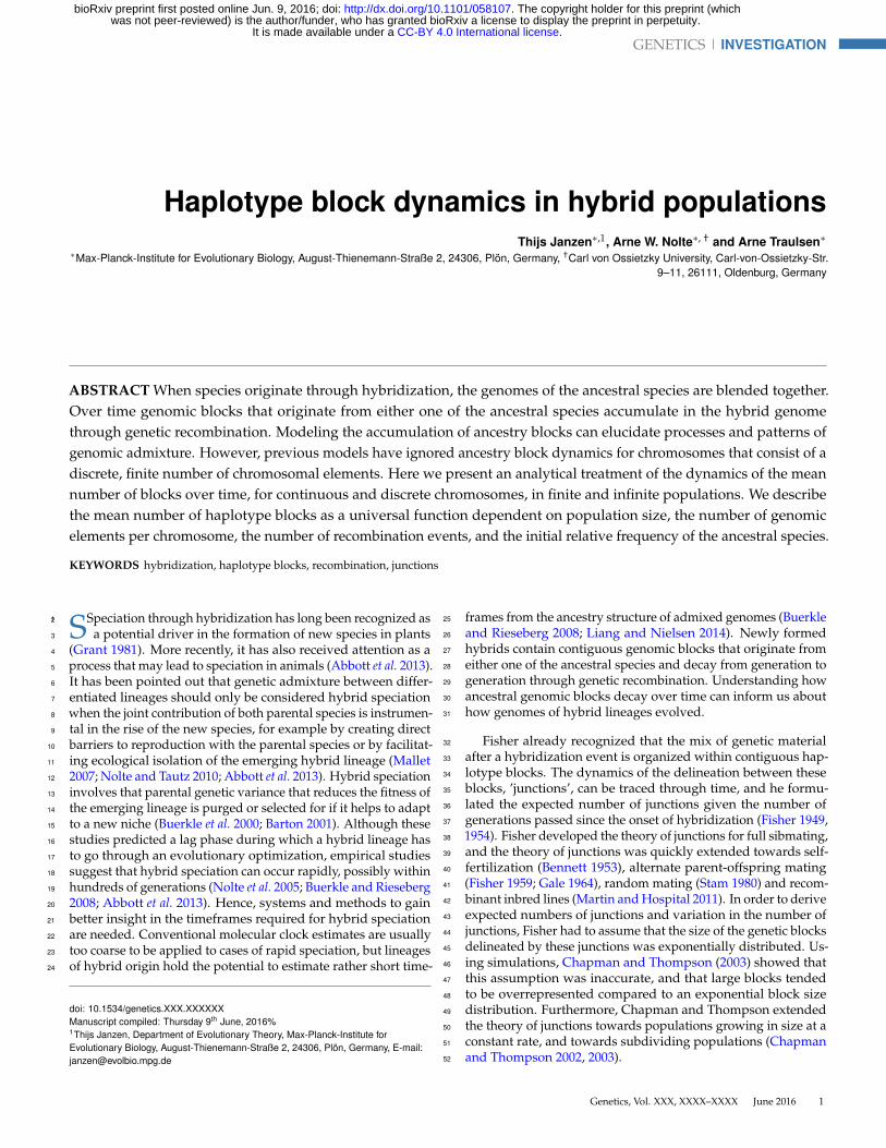
First, we derive the expected number of blocks depending on113

the time since the onset of hybridization. We assume infinite114

population size, random mating, and an continuous chromo-115

some, e.g. there are an infinite number of recombination sites116

along the chromosome. We assume that only a single crossover117

event occurs per chromosome per meiosis, which corresponds118

to the assumption that chromosomes are 1 Morgan long. The re-119

combination rate is assumed to be uniformly distributed across120

the chromosome. Both chromosomes are interchangeable, and121

we do not keep track of the identity of chromosomes. Each122

individual is diploid and chromosomes are inherited indepen-123

dently, which allows us to track haplotype blocks within only124

one chromosome pair, rather than all pairs simultaneously.125

We start by formulating a recurrence equation based on the126

expected change, or the change in mean number of blocks per127

generation. Given a recombination site picked randomly across128

the length of the chromosome, the genomic material on either129

chromosome can either be identical or different. If the genomic130

material is identical, no change in the number of blocks occurs.131

If the genomic material is different, a new block is formed (see132

Figure 1). The probability of observing the same type of genomic133

material on both chromosomes is proportional to the frequency134

of genomic material of that type in the population, which in turn135

is dependent on the frequency of the corresponding ancestral136

species in the ancestral population. We denote the frequency137

of type P genomic material from ancestral species 1 as p, and138

the frequency of genomic material of the other type Q (from the139

other ancestral species) as q, where p = 1− q. The probability of140

having the same type of genomic material on both chromosomes141

at the recombination site is then p2 + q2, in which case no change142

in the number of blocks is observed. With probability 2pq the143

type of genomic material on both chromosomes differs and an144

increase in number of blocks is observed. We obtain145

nt+1 = nt + 2pq. (1)

Here nt is the average number of blocks at time t. The solution146

of Equation (1) is given by147

nt = n0 + 2pqt. (2)

The number of blocks increases linear in time. The probability of148

having a different type of genomic material, 2pq, is the heterozy-149

gosity H, and we can write Equation (2) in terms of heterozy-150

gosity, nt = n0 + Ht. Taking into account that the number of151

junctions J at time t is Jt = nt − 1 and assuming a non-constant152

heterozygosity H, we recover the previously obtained result153

(Chapman and Thompson 2002; MacLeod et al. 2005; Buerkle154

and Rieseberg 2008)155

Jt =t−1

∑i=0

Hi, (3)

where Jt is the number of junctions J at time t. Because the156

population size is infinite, in our case the average heterozygosity157

does not change from H0, and Jt = H0t.158

If the population size is not infinite, but finite with size Nj159

at time j, and we allow for selfing, the average heterozygosity160

changes over time (Crow and Kimura 1970) as161

Hi = H0

i−1

∏j=0

(1− 1

2Nj

). (4)

2 Thijs Janzen et al.



http://dx.doi.org/10.1101/058107


Assuming constant population size, Nj = N for all j, the ex-162

pected number of junctions is given by163

Jt =t−1

∑i=0

Hi =t−1

∑i=0

H0

(1− 1

2N

)i−1. (5)

The expected number of blocks, given an initial proportion p of164

species 1 is given by:165

nt = 1 + 2pqt−1

∑j=0

(1− 1

2N

)j−1. (6)

In the limit of N → ∞ we recover Equation (2). For t→ ∞, we166

have (MacLeod et al. 2005)167

n∞ = 1 + 4pqN. (7)

Thus, for finite N, the number of blocks converges to a finite168

number determined only by the population size and the initial169

frequencies of genomic material, which in turn depends on the170

frequency of the ancestral species during the first admixture171

event.172

2pqp2 q2

Figure 1 Change in number of haplotype blocks dependingon the genomic match between blocks. Top row depicts thetwo parental chromosomes, bottom row depicts the two chro-mosomes produced after recombination has taken place at thegrey dotted line during meiosis. Genome types are indicatedusing either black color (type P), or white color (type Q).Withprobability p2 + q2 no change in the number of blocks is ob-served. With probability 2pq we observe an increase in thenumber of blocks, where p = 1− q is the fraction of genomicmaterial of type 1.

B. A finite number of recombination spots: a discrete chro-173

mosome174

In the previous section we have assumed that recombination175

never occurs twice at the same spot. In reality, a chromosome176

can not be indefinitely divided into smaller parts. We therefore177

proceed to study the change in number of blocks in a chromo-178

some consisting of L different chromosomal segments, where179

each segment represents a minimal genomic element that can not180

be broken down further, for instance a single nucleotide, a gene,181

a specific codon, or a genomic area delineated by two genetic182

markers. Considering a chromosome of L genomic segments,183

there are L− 1 possible crossover spots (junctions). Given that184

there are n blocks on the chromosome, there are n− 1 points on185

the chromosome where one block ends, and a new block begins186

(Fisher called these external junctions), excluding the tips of the187

chromosome. The probability that a recombination event takes188

place at exactly such a point, given that there are nt blocks at189

time t is:190

α =nt − 1L− 1

(8)

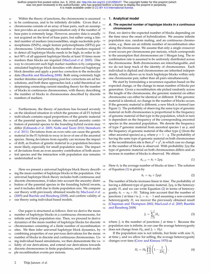
Conditioning on the type of the first chromosome, and only191

looking at the first of the two produced chromosomes (all other192

produced chromosomes are identical or the exact mirror image193

of this chromosome) we can distinguish four possible events,194

taking into account the location of the recombination spot on195

both chromosomes (Figure 2):196

A) recombination takes place on an existing junction on both197

chromosomes (probability α2)198

B) recombination takes place on an existing junction on one199

chromosome, and within a block on the other chromosome200

(probability α(1− α))201

C) recombination takes place on within a block on one chromo-202

some, and on an existing junction on the other chromosome203

(probability (1− α)α)204

D) recombination takes place within a block on both chromo-205

somes (probability (1− α)2)206

0.5α(1-α)0.5α(1-α) (p*2+q*2)(1-α)2 2p*q*(1-α)2

BA0.5α(1-α) 0.5α(1-α)

C D

0.5α2 0.5α2

Figure 2 Change in number of haplotype blocks dependingon the genomic match between blocks. Full chromosomesare shown here, but the same rationale applies to subsets ofa chromosome. Top rows within each panel indicate the twoparental chromosomes, bottom row indicates one of two possi-ble resulting chromosomes after meiosis, where recombinationtakes place at the dotted grey line. Genomic material of type1 is indicated in black, genomic material of type 2 is indicatedin white. With probability α2 recombination takes place on anexisting junction on both chromosomes A, with probabilityα(1 − α) recombination takes place on an existing junctionon one chromosome, and within a block on the other chromo-some B, with probability (1− α)α recombination takes placeon within a block on one chromosome, and on an existing junc-tion on the other chromosome C, with probability (1− α)2 re-combination takes place within a block on both chromosomesD.

A) When a crossover event takes place on an existing junction207

on both chromosomes, there is either no change in the number208

Haplotype block dynamics 3



http://dx.doi.org/10.1101/058107


of blocks (when the two junctions are identical), or a decrease in209

the number of blocks (when the two junctions are of opposing210

type). The probability of either event happening is 12 , yielding211

an average change in the number of blocks when crossover takes212

place on an exisiting junction on both chromosomes of − 12 .213

B) When a crossover event takes place on an existing junction214

on one chromosome, and within a block on the other chromo-215

some, there are two possibilities: either the block on the other216

chromosome is of the same type as the genomic material before217

the existing junction, or it is of the other type. If it is of the218

same type, the existing junction disappears, and the number of219

blocks decreases by one. If it is of the other type, the existing220

junction remains and the number of blocks does not change. The221

probability of either event happening is 12 , and hence we expect222

the total number of blocks on average to change by − 12 .223

C) When a crossover event takes place within a block on224

the first chromosome, and on an existing junction on the other225

chromosome (the inverse of the previous situation), the outcome226

is exactly the opposite. If the genetic material after the junction227

on the second chromosome is of the same type as the block on228

the first chromosome, no new junction is formed and the number229

of blocks stays the same. If the genetic material after the junction230

on the second chromosome is of a different type than that of the231

block on the first chromosome, a new junction is formed and232

the number of blocks increases by one. The probability of either233

event happening is 12 , and hence we expect the total number of234

blocks on average to change by 12 .235

D) When recombination takes place within a block on bothchromosomes, matters proceed as described for the continuouschromosome: with probability p2 + q2 we observe no changein the number of blocks, and with probability 2pq we observean increase. But, since we are dealing with a finite numberof junction positions along the chromosome, the frequency ofjunction spots of a genomic type is no longer directly related top. If there would be no blocks, i.e. if the genomic material wouldbe distributed in an uncorrelated way, we know that p(L− 1)junction spots are of type P, that is, they are within a block oftype P. Similarly, q(L− 1) junction spots are within a block oftype Q. As new blocks are formed, the number of junction spotsthat are still within a block decreases. With the formation of anew block, on average both a junction within a block of type Pand a junction within a block of type Q are lost, such that onaverage, after the formation of a new junction, the number ofjunctions of type P decreases by 1

2 (n − 1). Thus the numberof junctions within a block of type P is p(L − 1) − 1

2 (n − 1).Similarly, the number of junctions within a block of type Q isq(L− 1)− 1

2 (n− 1). The probability then of selecting an internaljunction of type P is the number of internal junctions of typeP divided by the total number of junctions. Let us denote theprobability of selecting an internal junction of type P by p∗,which is then given by

p∗t =p(L− 1)− 1

2 (nt − 1)

p(L− 1)− 12 (nt − 1) + q(L− 1)− 1

2 (nt − 1)

=p(L− 1)− 1

2 (nt − 1)L− nt

. (9)

And the probability q∗t is236

q∗t = 1− p∗t =q(L− 1)− 1

2 (nt − 1)L− nt

. (10)

With probability 2p∗t q∗t we observe an increase in number of237

blocks. Combining the scenarios (A)-(D) we can formulate the238

total expected change in number of blocks239

nt+1 = nt + 2p∗t q∗t (1− α)2 +12

α(1− α)− 12(α(1− α))− 1

2α2

= nt + 2p∗t q∗t (1− α)2 − 12

α2. (11)

In terms of p, q, and L, Equation (11) can be written as240

nt+1 = 2pq +1

L− 1+

L− 2L− 1

nt (12)

The solution of the recursion Equation (12) is given by

nt = n0

(L− 2L− 1

)t+ (1 + 2pq(L− 1))

(1−

(L− 2L− 1

)t)

. (13)

The exponential decay terms ensures that we have convergence241

at t→ ∞, where we obtain242

n∞ = 1 + 2pq(L− 1). (14)

A Taylor expansion at t = 0 shows that initially, the number of243

blocks increases linearly244

n ≈ n0 + (n0 − n∞) ln(

L− 2L− 1

)t. (15)

C. Multiple recombination events245

So far, we have assumed that during meiosis only a single246

crossover event occurs. Although this might often apply, multi-247

ple crossover events occur frequently. First, we consider the case248

of two crossover events. Assuming that the position of the two249

crossovers is independent, that there is no interference between250

the two crossovers, and that the two crossovers do not take place251

at the same position, we can extend our recurrence equations as252

follows.253

For an infinite population, with a discrete chromosome, the254

first position is still chosen as in Equation (11). To obtain the255

probability for the second position of selecting a junction that256

lies within two dissimilar blocks, we have to correct p∗t and q∗t257

(whereas previously there were L− 1 spots, there are now L− 2),258

and we obtain259

nt+1 = nt+

(2p∗1(t)q

∗1(t)(1− α1)

2 − 12

α21

)+(

2p∗2(t)q∗2(t)(1− α2)

2 − 12

α22

). (16)

Where:

p∗1(t) =p(L− 1)− 1

2 (nt − 1)L− nt

(17)

q∗1(t) =q(L− 1)− 1

2 (nt − 1)L− nt

(18)

p∗2(t) =p(L− 2)− 1

2 (nt − 1)L− nt − 1

(19)

q∗2(t) =q(L− 2)− 1

2 (nt − 1)L− nt − 1

(20)

α1 =(nt − 1)

L− 1(21)

α2 =(nt − 1)

L− 2. (22)




http://dx.doi.org/10.1101/058107


Equation (16) has the solution:

nt =n0

(L2 − 5L + 5

(L− 2)(L− 1)

)t

+(1 + 4pq

(L− 2)(L− 1)2L− 3

)(1−

(L2 − 5L + 5

(L− 2)(L− 1)

)t)(23)

Again we have convergence at t→ ∞, where we obtain:260

n∞ = 1 + 4pq(L− 1)(L− 2)

2L− 3≈ 1 + 2pq(L− 1), (24)

where the approximation holds for large L. The difference in themaximum number of blocks between one and two recombina-tion events is

n∞2 − n∞1 = 1 + 4pq(L− 1)(L− 2)

2L− 3− (1 + 2pq(L− 1))

= −2pqL− 1

2L− 3≈ −pq, (25)

where the approximation again holds for large L. An increase261

in the number of recombination events thus decreases the maxi-262

mum number of blocks.263

Extending Equation (16) towards M recombination events is264

similar,265

nt+1 = nt +M

∑i=1

(2p∗i q∗i (1− αi)

2 − 12

α2i

)(26)

with

pi =p(L− i)− 1

2 (nt − 1)

p(L− i)− 12 (nt − 1) + q(L− i)− 1

2 (nt − 1)(27)

qi =q(L− i)− 1

2 (nt − 1)

p(L− i)− 12 (nt − 1) + q(L− i)− 1

2 (nt − 1)(28)

αi =(nt − 1)

L− i. (29)

For not too small L, and not too large M, taking into accountEquation (25), we can approximate n∞ by:

n∞ = 1 + 2pq(L− 1)− 2pq(M− 1)L− 1

2L− 3(30)

≈ 1 + 2pq(L− 1)− pq(M− 1) (31)

Using numerical iteration of Equation (26) for M = [2, 3, 4, 5] and266

L = [2M + 1, 2M + 2, . . . , 200], and comparing the maximum267

number of blocks with the approximation of Equation (31) shows268

that Equation (31) is a good approximation (error < 0.1%) for269

L ≥ 10M− 3.270

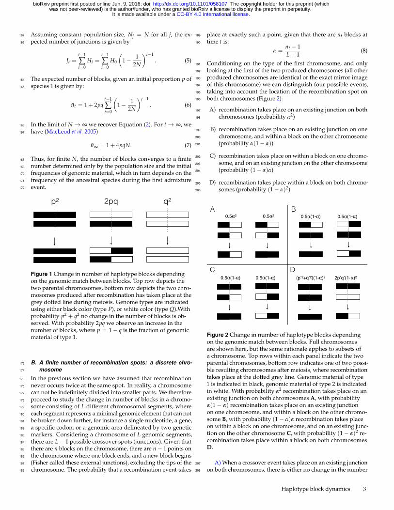
2. Universal haplotype dynamics271

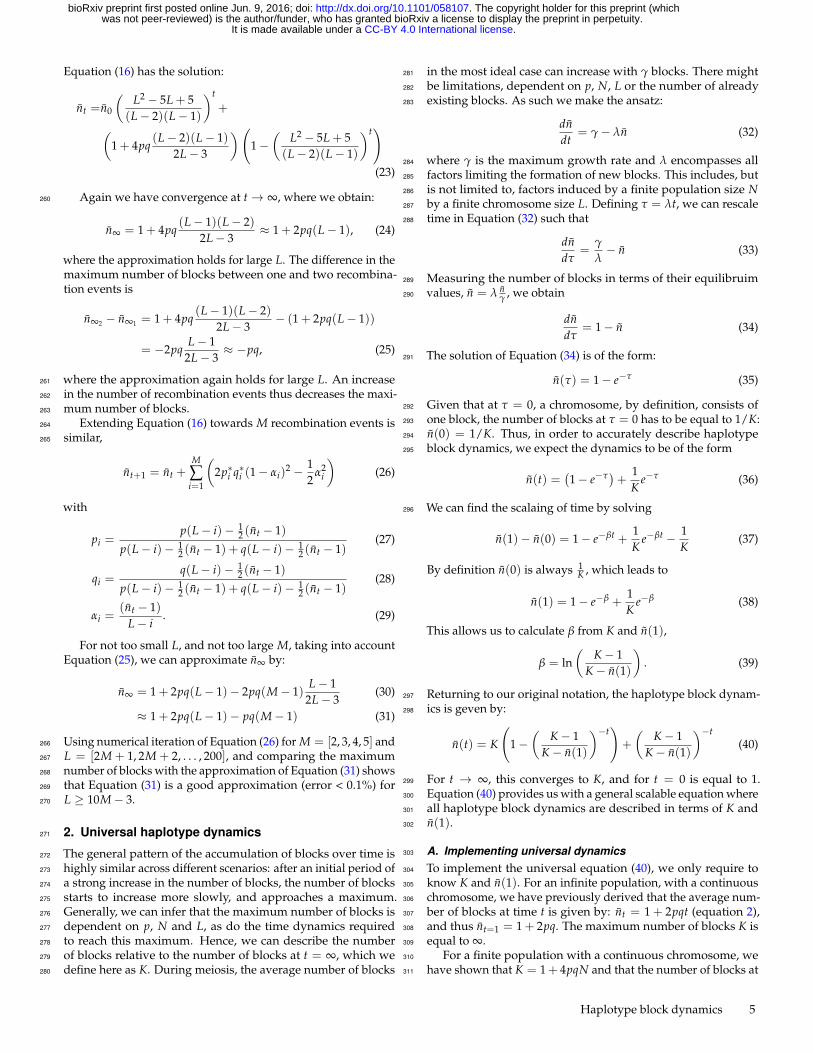
The general pattern of the accumulation of blocks over time is272

highly similar across different scenarios: after an initial period of273

a strong increase in the number of blocks, the number of blocks274

starts to increase more slowly, and approaches a maximum.275

Generally, we can infer that the maximum number of blocks is276

dependent on p, N and L, as do the time dynamics required277

to reach this maximum. Hence, we can describe the number278

of blocks relative to the number of blocks at t = ∞, which we279

define here as K. During meiosis, the average number of blocks280

in the most ideal case can increase with γ blocks. There might281

be limitations, dependent on p, N, L or the number of already282

existing blocks. As such we make the ansatz:283

dndt

= γ− λn (32)

where γ is the maximum growth rate and λ encompasses all284

factors limiting the formation of new blocks. This includes, but285

is not limited to, factors induced by a finite population size N286

by a finite chromosome size L. Defining τ = λt, we can rescale287

time in Equation (32) such that288

dndτ

=γ

λ− n (33)

Measuring the number of blocks in terms of their equilibruim289

values, n = λ nγ , we obtain290

dndτ

= 1− n (34)

The solution of Equation (34) is of the form:291

n(τ) = 1− e−τ (35)

Given that at τ = 0, a chromosome, by definition, consists of292

one block, the number of blocks at τ = 0 has to be equal to 1/K:293

n(0) = 1/K. Thus, in order to accurately describe haplotype294

block dynamics, we expect the dynamics to be of the form295

n(t) =(1− e−τ

)+

1K

e−τ (36)

We can find the scalaing of time by solving296

n(1)− n(0) = 1− e−βt +1K

e−βt − 1K

(37)

By definition n(0) is always 1K , which leads to

n(1) = 1− e−β +1K

e−β (38)

This allows us to calculate β from K and n(1),

β = ln(

K− 1K− n(1)

). (39)

Returning to our original notation, the haplotype block dynam-297

ics is geven by:298

n(t) = K

(1−

(K− 1

K− n(1)

)−t)+

(K− 1

K− n(1)

)−t(40)

For t → ∞, this converges to K, and for t = 0 is equal to 1.299

Equation (40) provides us with a general scalable equation where300

all haplotype block dynamics are described in terms of K and301

n(1).302

A. Implementing universal dynamics303

To implement the universal equation (40), we only require to304

know K and n(1). For an infinite population, with a continuous305

chromosome, we have previously derived that the average num-306

ber of blocks at time t is given by: nt = 1 + 2pqt (equation 2),307

and thus nt=1 = 1 + 2pq. The maximum number of blocks K is308

equal to ∞.309

For a finite population with a continuous chromosome, we310

have shown that K = 1+ 4pqN and that the number of blocks at311




http://dx.doi.org/10.1101/058107


0 200 400 600 800 1000 1200

Time

Num

ber

of B

lock

s

0

10

20

30

40

50

60

70

●

●

●●

●●●●●●●●●●●●●●●●●●●●●●●●●●●●●●●●●●●●●●●●●●●●●● N = 50 L = 50

●

●

●

●

●●

●●●●●●●●●●●●●●●●●●●●●●●●●●●●●●●●●●●●●●●●●●●● N = 50 L = 100

●

●

●

●

●

●●

●●●●●●●●●●●●●●●●●●●●●●●●●●●●●●●●●●●●●●●●●●●

N = 50 L = 200

●

●

●

●●

●●●●●●●●●●●●●●●●●●●●●●●●●●●●●●●●●●●●●●●●●●●●● N = 100 L = 50

●

●

●

●

●

●●

●●●●●●●●●●●●●●●●●●●●●●●●●●●●●●●●●●●●●●●●●●● N = 100 L = 100

●

●

●

●

●

●

●

●●

●●

●●●●●●●●●●●●●●●●●●●●●●●●●●●●●●●●●●●●●●● N = 100 L = 200

●

●

●

●●

●●●●●●●●●●●●●●●●●●●●●●●●●●●●●●●●●●●●●●●●●●●●● N = 200 L = 50

●

●

●

●

●

●

●●

●●●●●●●●●●●●●●●●●●●●●●●●●●●●●●●●●●●●●●●●●● N = 200 L = 100

●

●

●

●

●

●

●

●

●

●

●●

●●

●●●●●●●●●●●●●●●●●●●●●●●●●●●●●●●●●●●● N = 200 L = 200

A

0 200 400 600 800 1000

Time

Num

ber

of b

lock

s / m

axim

um n

umbe

r of

blo

cks

0.0

0.1

0.2

0.3

0.4

0.5

0.6

0.7

0.8

0.9

1.0

●

●

●

●

●

●● ● ● ● ● ● ● ● ● ● ● ● ● ● ● ● ● ● ● ● ● ● ● ● ● ● ● ● ● ● ● ● ● ● ● ● ● ● ● ● ● ● ● ●

●

●

●

●

●

●

●●

● ● ● ● ● ● ● ● ● ● ● ● ● ● ● ● ● ● ● ● ● ● ● ● ● ● ● ● ● ● ● ● ● ● ● ● ● ● ● ● ● ●

●

●

●

●

●

●

●

●●

●● ● ● ● ● ● ● ● ● ● ● ● ● ● ● ● ● ● ● ● ● ● ● ● ● ● ● ● ● ● ● ● ● ● ● ● ● ● ● ●

●

●

●

●

●

●●

● ● ● ● ● ● ● ● ● ● ● ● ● ● ● ● ● ● ● ● ● ● ● ● ● ● ● ● ● ● ● ● ● ● ● ● ● ● ● ● ● ● ●

●

●

●

●

●

●

●

●●

●● ● ● ● ● ● ● ● ● ● ● ● ● ● ● ● ● ● ● ● ● ● ● ● ● ● ● ● ● ● ● ● ● ● ● ● ● ● ● ●

●

●

●

●

●

●

●

●

●

●●

●●

●● ● ● ● ● ● ● ● ● ● ● ● ● ● ● ● ● ● ● ● ● ● ● ● ● ● ● ● ● ● ● ● ● ● ● ●

●

●

●

●

●

●

●●

● ● ● ● ● ● ● ● ● ● ● ● ● ● ● ● ● ● ● ● ● ● ● ● ● ● ● ● ● ● ● ● ● ● ● ● ● ● ● ● ● ●

●

●

●

●

●

●

●

●

●●

●●

● ● ● ● ● ● ● ● ● ● ● ● ● ● ● ● ● ● ● ● ● ● ● ● ● ● ● ● ● ● ● ● ● ● ● ● ● ●

●

●

●

●

●

●

●

●

●

●

●●

●●

●●

● ● ● ● ● ● ● ● ● ● ● ● ● ● ● ● ● ● ● ● ● ● ● ● ● ● ● ● ● ● ● ● ● ●B

0 2 4 6 8 10

Rescaled time

num

ber

of b

lock

s / m

axim

um n

umbe

r of

blo

cks

0.0

0.1

0.2

0.3

0.4

0.5

0.6

0.7

0.8

0.9

1.0

●

●

●

●

●

●

●

●

●

●●

●●

● ● ● ● ● ● ● ● ● ● ● ● ● ● ● ● ● ● ● ● ● ● ● ● ● ● ● ● ● ● ● ● ● ● ● ● ●

●

●

●

●

●

●

●

●

●

●●

●●

● ● ● ● ● ● ● ● ● ● ● ● ● ● ● ● ● ● ● ● ● ● ● ● ● ● ● ● ● ● ● ● ● ● ● ● ●

●

●

●

●

●

●

●

●

●

●●

●●

● ● ● ● ● ● ● ● ● ● ● ● ● ● ● ● ● ● ● ● ● ● ● ● ● ● ● ● ● ● ● ● ● ● ● ● ●

●

●

●

●

●

●

●

●

●

●●

●●

● ● ● ● ● ● ● ● ● ● ● ● ● ● ● ● ● ● ● ● ● ● ● ● ● ● ● ● ● ● ● ● ● ● ● ● ●

●

●

●

●

●

●

●

●

●

●●

●●

● ● ● ● ● ● ● ● ● ● ● ● ● ● ● ● ● ● ● ● ● ● ● ● ● ● ● ● ● ● ● ● ● ● ● ● ●

●

●

●

●

●

●

●

●

●

●●

●●

●● ● ● ● ● ● ● ● ● ● ● ● ● ● ● ● ● ● ● ● ● ● ● ● ● ● ● ● ● ● ● ● ● ● ● ●

●

●

●

●

●

●

●

●

●

●●

●●

● ● ● ● ● ● ● ● ● ● ● ● ● ● ● ● ● ● ● ● ● ● ● ● ● ● ● ● ● ● ● ● ● ● ● ● ●

●

●

●

●

●

●

●

●

●

●●

●●

● ● ● ● ● ● ● ● ● ● ● ● ● ● ● ● ● ● ● ● ● ● ● ● ● ● ● ● ● ● ● ● ● ● ● ● ●

●

●

●

●

●

●

●

●

●

●

●●

●●

●●

●●●●●●●●●●●●●●●●●●●●●●●●●●●●●●●●●●C

Figure 3 Graphical example of the construction of universalhaplotype block dynamics using results from individual basedsimulations. A: mean number of haplotype blocks for p = 0.5,N = [50, 100, 200] and L = [50, 100, 200], number of replicates= 10,000. B: The mean number of blocks for the same parame-ter combinations, after rescaling the number of blocks relativeto the maximum number of blocks K. C: The rescaled numberof blocks vs rescaled time, by rescaling time according to β inEquation (39). After rescaling both the number of blocks ac-cording to K, and time according to β, all curves for differentvalues of N and L reduce to a single, universal, curve, whichfollows Equation (40).

time t is given by nt = 1 + 2pq ∑t−1j=0(1−

12N )t−1 (Equation (6)),312

and hence nt=1 = 1 + 2pq.313

For an infinite population with a discrete chromosome,we have shown that K = 2pq(L − 1) + 1 and that the

number of blocks at time t is given by nt = n0

(L−2L−1

)t+

(2pq(L− 1) + 1)(

1−(

L−2L−1

)t)

(Equation (13)), and hence:

nt=1 =L− 2L− 1

+ (1 + 2pq(L− 1))(

1− L− 2L− 1

)=

L− 2L− 1

+ 1 + 2pq(L− 1)− (1 + 2pq(L− 1))L− 2L− 1

=L− 2L− 1

+ 1 + 2pq(L− 1)− 2pq(L− 2)− L− 2L− 1

= 1 + 2pq(L− 1)− 2pq(L− 2)

= 1 + 2pq. (41)

We find that regardless whether the chromosome is continuous314

or discrete, and regardless of whether the population is finite315

on infinite, n(1) = 1 + 2pq, which makes intuitive sense: in the316

first generation, none of the factors that limit recombination as a317

result of finite population size, or finite chromosome size come318

into play. When the population is finite, the formation of new319

blocks is limited by recombination taking place at a recombi-320

nation spot where in a previous generation recombination has321

already taken place. In the first generation, all chromosomes322

are non-recombined, and finite population effects have no effect323

yet. When the chromosome is discrete, the formation of new324

blocks is limited by recombination taking place on a site that325

has previously recombined. In the first generation, no previous326

recombination events have happened yet, and recombination is327

thus not limited (yet).328

3. Individual based simulations329

To verify our analytical framework, and extend the framework330

towards discrete chromosomes in finite populations, we test331

our findings using an individual based model. We model the332

hybrid population as a Wright-Fisher process, extended with333

recombination:334

• Non-overlapping generations335

• Constant population size N336

• Random mating337

• Diploid338

• Uniform recombination rate across the genome339

• M recombination events per meiosis340

Each individual has 2 chromosomes of length L, which are a341

sequence of 0 and 1’s, where 1 represents an allele from an an-342

cestral parent of type P and a 0 represents and allele from an343

ancestral parent of type Q. The model works as follows. In the344

first time step, N individuals are generated, where each individ-345

ual can have either two parents of type P (with probability p2),346

two parents of type Q (with probability (1− p)2) or one parent347

of type P and one parent of type Q (with probability 2p(1− p)).348

In every consecutive time step, N new individuals are pro-349

duced, where each individual is the product of a reproduction350

event between two individuals (including selfing) from the pre-351

vious generation. Parental individuals are drawn with replace-352

ment, such that one individual could reproduce multiple times,353

but will on average reproduce one time. We assume that in a354

mating event both parents produce a large number of haploid355




http://dx.doi.org/10.1101/058107


gametes from which two gametes (one from each parent) are356

chosen to form the new offspring. During production of the357

gametes, M recombination sites are chosen. The location of the358

recombination sites follows a uniform distribution between 0359

and L.360

A. Continuous Chromosome361

We model each chromosome as a continuous line, and only keep362

track of junctions delineating the end of a block. For each junc-363

tion, we record the position along the chromosome (a number364

between 0 and 1) and whether the transition is 0→ 1 or 1→ 0.365

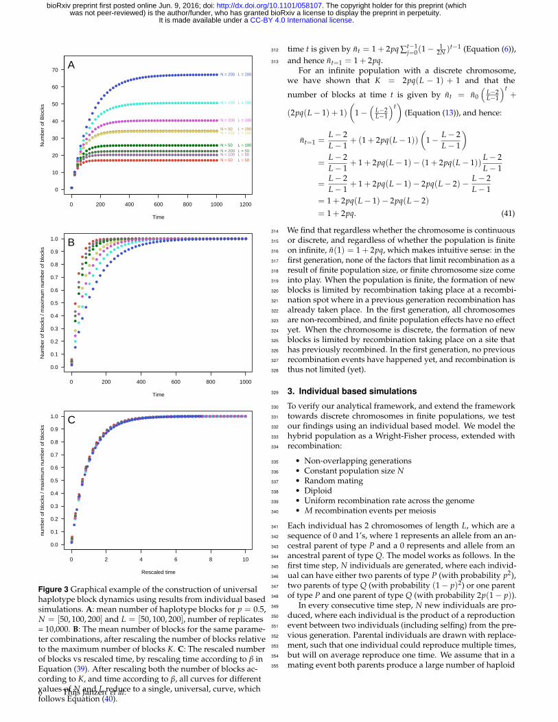
Over time, the number of blocks reaches a maximum value, but366

only if the population is finite (Figure 4). In the first few gen-367

erations the accumulation of blocks follows that of an infinite368

population (dotted line in Figure 4), but rapidly simulation re-369

sults start deviating from the infinite population dynamics. The370

maximum number of blocks is roughly obtained within 10N371

generations. Furthermore, when the amount of genetic mate-372

rial from either of the ancestral species is strongly skewed (e.g.373

p = 0.9), the maximum number of blocks is lower, and is reached374

within a shorter timespan.375

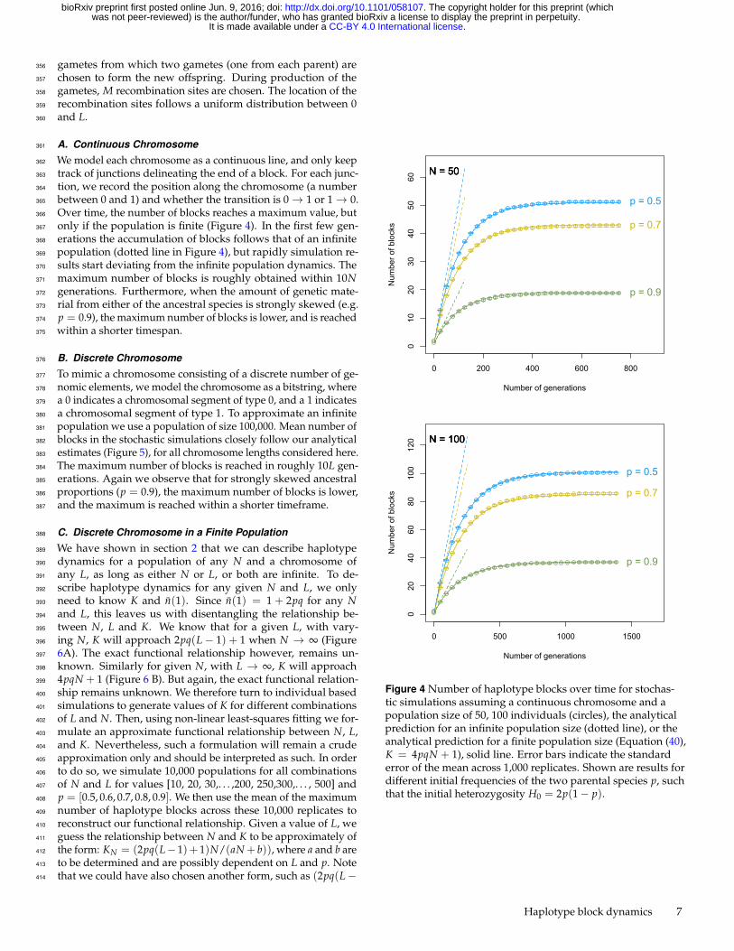
B. Discrete Chromosome376

To mimic a chromosome consisting of a discrete number of ge-377

nomic elements, we model the chromosome as a bitstring, where378

a 0 indicates a chromosomal segment of type 0, and a 1 indicates379

a chromosomal segment of type 1. To approximate an infinite380

population we use a population of size 100,000. Mean number of381

blocks in the stochastic simulations closely follow our analytical382

estimates (Figure 5), for all chromosome lengths considered here.383

The maximum number of blocks is reached in roughly 10L gen-384

erations. Again we observe that for strongly skewed ancestral385

proportions (p = 0.9), the maximum number of blocks is lower,386

and the maximum is reached within a shorter timeframe.387

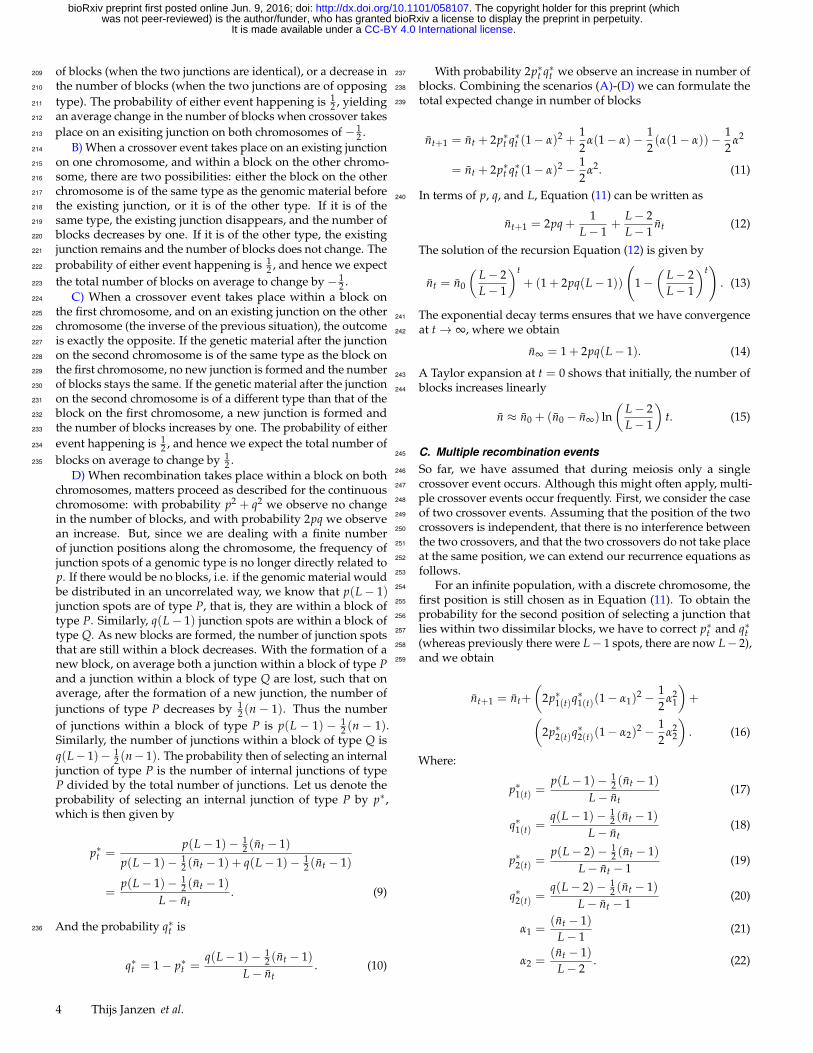
C. Discrete Chromosome in a Finite Population388

We have shown in section 2 that we can describe haplotype389

dynamics for a population of any N and a chromosome of390

any L, as long as either N or L, or both are infinite. To de-391

scribe haplotype dynamics for any given N and L, we only392

need to know K and n(1). Since n(1) = 1 + 2pq for any N393

and L, this leaves us with disentangling the relationship be-394

tween N, L and K. We know that for a given L, with vary-395

ing N, K will approach 2pq(L− 1) + 1 when N → ∞ (Figure396

6A). The exact functional relationship however, remains un-397

known. Similarly for given N, with L → ∞, K will approach398

4pqN + 1 (Figure 6 B). But again, the exact functional relation-399

ship remains unknown. We therefore turn to individual based400

simulations to generate values of K for different combinations401

of L and N. Then, using non-linear least-squares fitting we for-402

mulate an approximate functional relationship between N, L,403

and K. Nevertheless, such a formulation will remain a crude404

approximation only and should be interpreted as such. In order405

to do so, we simulate 10,000 populations for all combinations406

of N and L for values [10, 20, 30,. . . ,200, 250,300,. . . , 500] and407

p = [0.5, 0.6, 0.7, 0.8, 0.9]. We then use the mean of the maximum408

number of haplotype blocks across these 10,000 replicates to409

reconstruct our functional relationship. Given a value of L, we410

guess the relationship between N and K to be approximately of411

the form: KN = (2pq(L− 1)+ 1)N/(aN + b)), where a and b are412

to be determined and are possibly dependent on L and p. Note413

that we could have also chosen another form, such as (2pq(L−414

0 200 400 600 800

010

2030

4050

60

Number of generationsN

umbe

r of b

lock

s

p = 0.5

N = 50

p = 0.7

N = 50

p = 0.9

N = 50

0 500 1000 1500

020

4060

80100

120

Number of generations

Num

ber o

f blo

cks

p = 0.5

N = 100

p = 0.7

N = 100

p = 0.9

N = 100

Figure 4 Number of haplotype blocks over time for stochas-tic simulations assuming a continuous chromosome and apopulation size of 50, 100 individuals (circles), the analyticalprediction for an infinite population size (dotted line), or theanalytical prediction for a finite population size (Equation (40),K = 4pqN + 1), solid line. Error bars indicate the standarderror of the mean across 1,000 replicates. Shown are results fordifferent initial frequencies of the two parental species p, suchthat the initial heterozygosity H0 = 2p(1− p).




http://dx.doi.org/10.1101/058107


0 100 200 300 400 500 600

05

1015

2025

30

Number of Generations

Num

ber o

f Blo

cks

p = 0.5

L = 50

p = 0.7

L = 50

p = 0.9

L = 50

0 200 400 600 800 1000

010

2030

4050

60

Number of Generations

Num

ber o

f Blo

cks

p = 0.5

L = 100

p = 0.7

L = 100

p = 0.9

L = 100

Figure 5 Number of haplotype blocks over time for eitherstochastic simulations assuming a continuous chromosomeand a population size of 100,000 (circles), or the analyticalprediction according to Equation (40), K = 2pq(L − 1) + 1(solid line). Error bars indicate the standard error of the meanacross 100 replicates. Shown are results for different initialfrequencies of the two parental species p, such that the initialheterozygosity H0 = 2p(1− p).

1) + 1)(1− 1/(aN)b) or (2pq(L − 1) + 1)(1− exp(−aN + b)),415

however, we found KN = (2pq(L− 1) + 1)N/(aN + b)), to be416

easiest to fit to the data. Using non-linear least squares esti-417

mation we find that for L = 100 and p = 0.5, a = 1.014 and418

b = 47.83 (Figure 6 A). We can repeat this process for differ-419

ent values of L (but keeping p = 0.5) and find that a is always420

close to 1 and that b is always close to 2pq(L− 1) + 1. Hence,421

it makes more sense to find our approximation in the form:422

KN = c(2pq(L − 1) + 1)N/(aN + (2pq(L − 1) + 1))) (fitting423

more than 2 parameters at the same time tends to lead to in-424

accurate results). We find, by fitting to varying values of N425

and p, that a and c both tend to 4pq. With that, we obtain the426

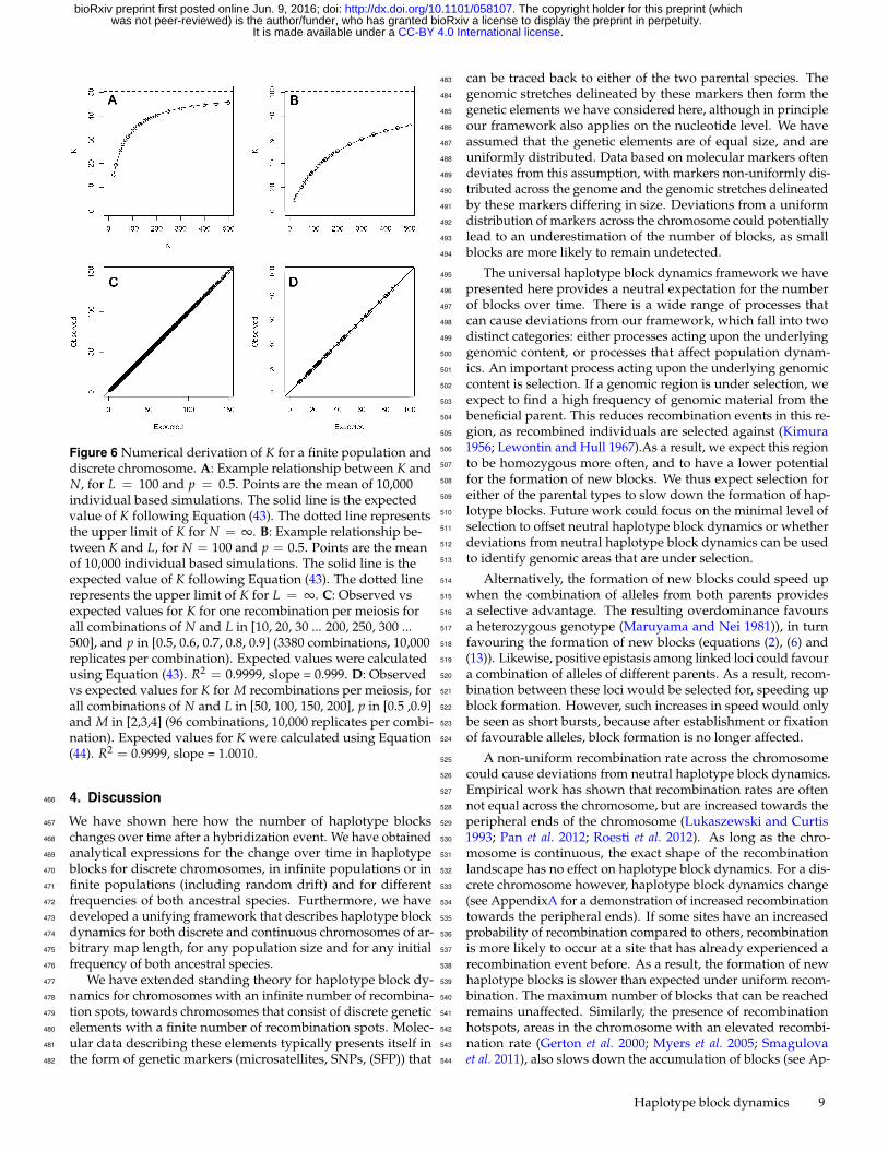
approximation for K:427

K =4pqN (1 + 2pq(L− 1))

4pqN + 1 + 2pq(L− 1)). (42)

We recover both limits of K for N → ∞ and L→ ∞, and formu-428

late our general approximation as:429

K =(1 + 4pqN)(1 + 2pq(L− 1))

2 + 4pqN + 2pq(L− 1)(43)

Comparing values of K expected following Equation (43) with430

the observed mean estimates from the simulations confirms that431

our approximation provides estimates that are close to the mean432

estimates (Figure 6 C, Observed vs Expected, intercept = -0.0727,433

slope = 0.9987, R2 = 0.9999).Furthermore, equation (43) reduces434

to Equation (7) when L � N, and reduces to Equation (14)435

when N � L. As such, Equation (43), albeit an approximation436

for K, encompasses all combinations of N and L. To extend437

Equation (43) towards M recombinations per meiosis, e.g. to438

chromosomes of any maplength in Morgan, we can suffice with439

a more sparse grid. Here we only need to show (numerically)440

that we can correct K for M recombinations, and substitute the441

corresponding equations into Equation (43). It has been shown442

previously that K, for L → ∞ is given by: K = 4pqMN + 1443

(Buerkle and Rieseberg 2008) and K for N → ∞ is given by:444

K = 2pq(L− 1) + 1− pq(M− 1) (Equation (31)). Substituting445

these expressions for K into Equation (43) we obtain446

K =(1 + 4pqMN)(1 + 2pq(L− 1)− (M− 1)pq)

2 + 4pqMN + 2pq(L− 1)− (M− 1)pq. (44)

We simulate values of K for combinations of N and L in [50,447

100, 150, 200], p in [0.5, 0.9] and M in [2,3,4]. We find that448

results from individual based simulations are very close to our449

predicted equation (Figure 6, intercept = -0.1352, slope = 1.0010,450

R2 = 0.9999). Equation (44), just like Equation (43), reduces to451

K = 4pqMN + 1 for L� N, and reduces to K = 2pqM(L− 1) +452

1− pq(M− 1) for N � L.453

As a further test of the accuracy of Equation (44), we repeat454

simulating values of K, but for more typical maplengths found455

in molecular data M = [0.5, 0.75, 1, 1.25, 1.5, 1.75, 2] (using456

the same sparse grid for N, L and p). We interpret fractional457

numbers of recombinations as a mean rate, such that an average458

of 1.25 recombinations implies that in 25% of all meiosis events459

there are 2 recombinations, and in 75% of all meiosis events460

there is 1 recombination. Again we find that obtained mean461

estimates for K are close to those predicted using Equation (44)462

(intercept = -0.2618, slope = 1.0027, R2 = 0.9999, not shown in463

Figure 6).464

465




http://dx.doi.org/10.1101/058107


A B

C D

Figure 6 Numerical derivation of K for a finite population anddiscrete chromosome. A: Example relationship between K andN, for L = 100 and p = 0.5. Points are the mean of 10,000individual based simulations. The solid line is the expectedvalue of K following Equation (43). The dotted line representsthe upper limit of K for N = ∞. B: Example relationship be-tween K and L, for N = 100 and p = 0.5. Points are the meanof 10,000 individual based simulations. The solid line is theexpected value of K following Equation (43). The dotted linerepresents the upper limit of K for L = ∞. C: Observed vsexpected values for K for one recombination per meiosis forall combinations of N and L in [10, 20, 30 ... 200, 250, 300 ...500], and p in [0.5, 0.6, 0.7, 0.8, 0.9] (3380 combinations, 10,000replicates per combination). Expected values were calculatedusing Equation (43). R2 = 0.9999, slope = 0.999. D: Observedvs expected values for K for M recombinations per meiosis, forall combinations of N and L in [50, 100, 150, 200], p in [0.5 ,0.9]and M in [2,3,4] (96 combinations, 10,000 replicates per combi-nation). Expected values for K were calculated using Equation(44). R2 = 0.9999, slope = 1.0010.

4. Discussion466

We have shown here how the number of haplotype blocks467

changes over time after a hybridization event. We have obtained468

analytical expressions for the change over time in haplotype469

blocks for discrete chromosomes, in infinite populations or in470

finite populations (including random drift) and for different471

frequencies of both ancestral species. Furthermore, we have472

developed a unifying framework that describes haplotype block473

dynamics for both discrete and continuous chromosomes of ar-474

bitrary map length, for any population size and for any initial475

frequency of both ancestral species.476

We have extended standing theory for haplotype block dy-477

namics for chromosomes with an infinite number of recombina-478

tion spots, towards chromosomes that consist of discrete genetic479

elements with a finite number of recombination spots. Molec-480

ular data describing these elements typically presents itself in481

the form of genetic markers (microsatellites, SNPs, (SFP)) that482

can be traced back to either of the two parental species. The483

genomic stretches delineated by these markers then form the484

genetic elements we have considered here, although in principle485

our framework also applies on the nucleotide level. We have486

assumed that the genetic elements are of equal size, and are487

uniformly distributed. Data based on molecular markers often488

deviates from this assumption, with markers non-uniformly dis-489

tributed across the genome and the genomic stretches delineated490

by these markers differing in size. Deviations from a uniform491

distribution of markers across the chromosome could potentially492

lead to an underestimation of the number of blocks, as small493

blocks are more likely to remain undetected.494

The universal haplotype block dynamics framework we have495

presented here provides a neutral expectation for the number496

of blocks over time. There is a wide range of processes that497

can cause deviations from our framework, which fall into two498

distinct categories: either processes acting upon the underlying499

genomic content, or processes that affect population dynam-500

ics. An important process acting upon the underlying genomic501

content is selection. If a genomic region is under selection, we502

expect to find a high frequency of genomic material from the503

beneficial parent. This reduces recombination events in this re-504

gion, as recombined individuals are selected against (Kimura505

1956; Lewontin and Hull 1967).As a result, we expect this region506

to be homozygous more often, and to have a lower potential507

for the formation of new blocks. We thus expect selection for508

either of the parental types to slow down the formation of hap-509

lotype blocks. Future work could focus on the minimal level of510

selection to offset neutral haplotype block dynamics or whether511

deviations from neutral haplotype block dynamics can be used512

to identify genomic areas that are under selection.513

Alternatively, the formation of new blocks could speed up514

when the combination of alleles from both parents provides515

a selective advantage. The resulting overdominance favours516

a heterozygous genotype (Maruyama and Nei 1981)), in turn517

favouring the formation of new blocks (equations (2), (6) and518

(13)). Likewise, positive epistasis among linked loci could favour519

a combination of alleles of different parents. As a result, recom-520

bination between these loci would be selected for, speeding up521

block formation. However, such increases in speed would only522

be seen as short bursts, because after establishment or fixation523

of favourable alleles, block formation is no longer affected.524

A non-uniform recombination rate across the chromosome525

could cause deviations from neutral haplotype block dynamics.526

Empirical work has shown that recombination rates are often527

not equal across the chromosome, but are increased towards the528

peripheral ends of the chromosome (Lukaszewski and Curtis529

1993; Pan et al. 2012; Roesti et al. 2012). As long as the chro-530

mosome is continuous, the exact shape of the recombination531

landscape has no effect on haplotype block dynamics. For a dis-532

crete chromosome however, haplotype block dynamics change533

(see AppendixA for a demonstration of increased recombination534

towards the peripheral ends). If some sites have an increased535

probability of recombination compared to others, recombination536

is more likely to occur at a site that has already experienced a537

recombination event before. As a result, the formation of new538

haplotype blocks is slower than expected under uniform recom-539

bination. The maximum number of blocks that can be reached540

remains unaffected. Similarly, the presence of recombination541

hotspots, areas in the chromosome with an elevated recombi-542

nation rate (Gerton et al. 2000; Myers et al. 2005; Smagulova543

et al. 2011), also slows down the accumulation of blocks (see Ap-544




http://dx.doi.org/10.1101/058107


pendix B for a demonstration of the effect of hotspots). Similar545

to increased recombination rates towards the peripheral ends,546

hotspots skew the recombination rate distribution to such an547

extend that recombination is much more likely to take place at a548

site that has been previously recombined, in which case no new549

block is formed.550

Apart from processes that act upon the genomic content, pop-551

ulation level processes are also expected to affect haplotype block552

dynamics. Firstly, deviations from having a constant-population553

size over time are expected to cause deviations from our hap-554

lotype block dynamics framework. A natural extension of our555

work would for instance be to include either exponentially or556

logistically growing populations in order to mimic real life dy-557

namics more closely. In exponentially growing populations,558

the average heterozygosity does not change (Crow and Kimura559

1970), which results in dynamics that resemble an infinite pop-560

ulation. Similarly, for logistically growing populations, during561

the initial growth phase, haplotype block dynamics are expected562

to closely resemble block dynamics in an infinite population. We563

do have to take into account that even though the population564

is growing exponentially, drift effects could interfere and cause565

deviations from infinite population dynamics (Hallatschek et al.566

2007). How drift and the rate of growth interact and influence567

haplotype block dynamics remains the subject of future study.568

Furthermore, in a growing population, the effect of selection569

is enhanced (Otto and Whitlock 1997), suggesting important570

interactions between selection, drift and population dynamics.571

Secondly, population subdivision, founder effects, a bottle-572

neck or a permanent decrease in population size could speed573

up fixation of haplotype blocks in the population through drift.574

Because haplotype blocks become fixed, the average heterozy-575

gosity decreases faster than expected, and the accumulation576

of new blocks is slowed down. Furthermore, the maximum577

number of blocks decreases as well (following Equation 43). De-578

pending on the speed and timing of the decrease, individuals579

in the final population potentially display a larger number of580

blocks than expected from the current population size, retaining581

blocks fixed in the population before the population decreased582

in size.583

Thirdly, secondary introgression, where admixture with the584

parental population after founding the hybrid population takes585

place, will affect haplotype block dynamics. Secondary intro-586

gression introduces new parental chromosomes that have not587

yet recombined and leads to an apparent reduction of the num-588

ber of blocks (Pool and Nielsen 2009). The apparent reduction589

of the mean number of blocks effectively ’turns back time’. A590

secondary introgression event introduces haplotype blocks that591

are disproportionally large, compared to the standing haplo-592

type block size distribution. As such, the haplotype block size593

distribution can potentially complement the mean number of594

blocks for inferring processes influencing genomic admixture595

after hybridization (Pool and Nielsen 2009).596

Apart from the before mentioned processes, we expect that597

there are more processes that can affect the accumulation of598

blocks, including, but not limited to, sib-mating, interference599

between recombination events, mutation, segregation distortion600

and heterochiasmy. Except for overdominance or positive epista-601

sis, all processes mentioned above slow down the accumulation602

of haplotype blocks. This suggests that the universal frame-603

work for haplotype block dynamics that we have presented here604

provides an upper limit to haplotype block dynamics.605

Similar to punctuated admixture events that we have consid-606

ered here, repeated or continuous gene flow between popula-607

tions can result in haplotype block structures, where the genomic608

material of the blocks can be traced back to distinct populations609

(Payseur and Rieseberg 2016), but where secondary migrants610

introduce disproportionally large haplotype blocks into the pop-611

ulation (Harris and Nielsen 2013; Liang and Nielsen 2014). How-612

ever, in between migration or phases of increased admixture,613

the introduced genomic material breaks down into blocks, fol-614

lowing similar dynamics as in our framework. Gravel has ex-615

plored the impact of past migration events on the block size616

distribution, and was able to use the block size distribution to617

infer past migration events of human populations from genome618

data (Gravel 2012). Further studies have extended his approach,619

and increased the accuracy of inference, and extended his ap-620

proach towards inferring effective population size and popu-621

lation substructuring (Palamara et al. 2012; Harris and Nielsen622

2013; Hellenthal et al. 2014; Sedghifar et al. 2016). These studies623

rely on simulations in combination with likelihood methods624

to infer migration events from empirical data. Our framework625

complements that approach, contributes to a more complete un-626

derstanding of the processes driving haplotype block dynamics.627

We have shown here how the genomic material of two628

parental species mixes over time after a hybridization event.629

With the current advances in genomic methods, it is now pos-630

sible, and affordable, to screen species for recurring haplotype631

blocks of other, closely related, species. Our framework can632

then be used inversely, by inferring the time of the hybridization633

event. Given that there are many processes that can potentially634

slow down the accumulation of haplotype blocks, inferring the635

time of hybridization using our universal haplotype block dy-636

namics framework provides the lower time limit, e.g. the mini-637

mum age of the hybrid. Caution should be taken however, as638

our work shows that haplotype block dynamics tend to stabilize639

relatively quickly (on an evolutionary timescale), where typi-640

cally the number of blocks reaches a maximum limit in the order641

of 10N or 10L generations. As a result, haplotype block patterns642

are especially useful for recent hybridization events.643

5. Data availability644

Computer code used for the individual based simulations645

has been made available on GitHub and can be found on:646

https://github.com/thijsjanzen/Haplotype-Block-Dynamics647

Literature Cited648

Abbott, R., D. Albach, S. Ansell, J. W. Arntzen, S. J. E. Baird,649

N. Bierne, J. Boughman, A. Brelsford, C. A. Buerkle, R. Buggs,650

R. K. Butlin, U. Dieckmann, F. Eroukhmanoff, A. Grill, S. H.651

Cahan, J. S. Hermansen, G. Hewitt, A. G. Hudson, C. Jig-652

gins, J. Jones, B. Keller, T. Marczewski, J. Mallet, P. Martinez-653

Rodriguez, M. Möst, S. Mullen, R. Nichols, A. W. Nolte,654

C. Parisod, K. Pfennig, A. M. Rice, M. G. Ritchie, B. Seifert,655

C. M. Smadja, R. Stelkens, J. M. Szymura, R. Väinölä, J. B. W.656

Wolf, and D. Zinner, 2013 Hybridization and speciation. Jour-657

nal of Evolutionary Biology 26: 229–246.658

Arbeithuber, B., A. J. Betancourt, T. Ebner, and I. Tiemann-Boege,659

2015 Crossovers are associated with mutation and biased gene660

conversion at recombination hotspots. Proceedings of the Na-661

tional Academy of Sciences 112: 2109–2114.662

Barton, N., 2001 The role of hybridization in evolution. Molecu-663

lar Ecology 10: 551–568.664

Bennett, J., 1953 Junctions in inbreeding. Genetica 26: 392–406.665




http://dx.doi.org/10.1101/058107


Buerkle, C. A., R. J. Morris, M. A. Asmussen, and L. H. Rieseberg,666

2000 The likelihood of homoploid hybrid speciation. Heredity667

84: 441–451.668

Buerkle, C. A. and L. H. Rieseberg, 2008 The rate of genome669

stabilization in homoploid hybrid species. Evolution 62: 266–670

275.671

Chapman, N. and E. Thompson, 2003 A model for the length of672

tracts of identity by descent in finite random mating popula-673

tions. Theoretical Population Biology 64: 141–150.674

Chapman, N. H. and E. A. Thompson, 2002 The effect of popula-675

tion history on the lengths of ancestral chromosome segments.676

Genetics 162: 449–458.677

Crow, J. F. and M. Kimura, 1970 An Introduction to Population678

Genetics Theory. Harper and Row, New York.679

Edmands, S., H. Feaman, J. Harrison, and C. Timmerman, 2005680

Genetic consequences of many generations of hybridization681

between divergent copepod populations. Journal of Heredity682

96: 114–123.683

Fisher, R. A., 1949 The Theory of Inbreeding. Oliver and Boyd.684

Fisher, R. A., 1954 A fuller theory of "junctions" in inbreeding.685

Heredity 8: 187–197.686

Fisher, R. A., 1959 An algebraically exact examination of junction687

formation and transmission in parent-offspring inbreeding.688

Heredity 13: 179–186.689

Gale, J., 1964 Some applications of the theory of junctions. Bio-690

metrics pp. 85–117.691

Gerton, J. L., J. DeRisi, R. Shroff, M. Lichten, P. O. Brown, and692

T. D. Petes, 2000 Global mapping of meiotic recombination693

hotspots and coldspots in the yeast saccharomyces cerevisiae.694

Proceedings of the National Academy of Sciences 97: 11383–695

11390.696

Grant, V., 1981 Plant speciation. Columbia University Press.697

Gravel, S., 2012 Population genetics models of local ancestry.698

Genetics 191: 607–619.699

Hallatschek, O., P. Hersen, S. Ramanathan, and D. R. Nelson,700

2007 Genetic drift at expanding frontiers promotes gene segre-701

gation. Proceedings of the National Academy of Sciences 104:702

19926–19930.703

Harris, K. and R. Nielsen, 2013 Inferring demographic history704

from a spectrum of shared haplotype lengths. PLoS Genetics705

9: e1003521.706

Hellenthal, G., G. B. Busby, G. Band, J. F. Wilson, C. Capelli,707

D. Falush, and S. Myers, 2014 A genetic atlas of human admix-708

ture history. Science 343: 747–751.709

Kimura, M., 1956 A model of a genetic system which leads to710

closer linkage by natural selection. Evolution pp. 278–287.711

Lewontin, R. and P. Hull, 1967 The interaction of selection and712

linkage iii synergistic effect of blocks of genes. Der Züchter 37:713

93–98.714

Liang, M. and R. Nielsen, 2014 The lengths of admixture tracts.715

Genetics 197: 953–967.716

Lukaszewski, A. and C. Curtis, 1993 Physical distribution of717

recombination in b-genome chromosomes of tetraploid wheat.718

Theoretical and Applied Genetics 86: 121–127.719

Mackiewicz, D., P. M. C. de Oliveira, S. M. de Oliveira, and720

S. Cebrat, 2013 Distribution of recombination hotspots in the721

human genome–a comparison of computer simulations with722

real data. PloS ONE 8: e65272.723

MacLeod, A., C. Haley, J. Woolliams, and P. Stam, 2005 Marker724

densities and the mapping of ancestral junctions. Genetical725

research 85: 69–79.726

Mallet, J., 2007 Hybrid speciation. Nature 446: 279–283.727

Martin, O. C. and F. Hospital, 2011 Distribution of parental728

genome blocks in recombinant inbred lines. Genetics 189: 645–729

654.730

Maruyama, T. and M. Nei, 1981 Genetic variability maintained731

by mutation and overdominant selection in finite populations.732

Genetics 98: 441–459.733

McVean, G. A., S. R. Myers, S. Hunt, P. Deloukas, D. R. Bentley,734

and P. Donnelly, 2004 The fine-scale structure of recombination735

rate variation in the human genome. Science 304: 581–584.736

Myers, S., L. Bottolo, C. Freeman, G. McVean, and P. Donnelly,737

2005 A fine-scale map of recombination rates and hotspots738

across the human genome. Science 310: 321–324.739

Nolte, A. W., J. Freyhof, K. C. Stemshorn, and D. Tautz, 2005740

An invasive lineage of sculpins, cottus sp. (pisces, teleostei) in741

the rhine with new habitat adaptations has originated from742

hybridization between old phylogeographic groups. Proceed-743

ings of the Royal Society B 272: 2379–2387.744

Nolte, A. W. and D. Tautz, 2010 Understanding the onset of745

hybrid speciation. Trends in Genetics 26: 54–58.746

Otto, S. P. and M. C. Whitlock, 1997 The probability of fixation747

in populations of changing size. Genetics 146: 723–733.748

Palamara, P. F., T. Lencz, A. Darvasi, and I. Pe’er, 2012 Length749

distributions of identity by descent reveal fine-scale demo-750

graphic history. The American Journal of Human Genetics 91:751

809–822.752

Pan, Q., F. Ali, X. Yang, J. Li, and J. Yan, 2012 Exploring the753

genetic characteristics of two recombinant inbred line pop-754

ulations via high-density snp markers in maize. PLoS ONE755

7.756

Payseur, B. A. and L. H. Rieseberg, 2016 A genomic perspective757

on hybridization and speciation. Molecular Ecology .758

Pool, J. E. and R. Nielsen, 2009 Inference of historical changes759

in migration rate from the lengths of migrant tracts. Genetics760

181: 711–719.761

Roesti, M., A. P. Hendry, W. Salzburger, and D. Berner, 2012762

Genome divergence during evolutionary diversification as763

revealed in replicate lake–stream stickleback population pairs.764

Molecular Ecology 21: 2852–2862.765

Sedghifar, A., Y. Brandvain, and P. Ralph, 2016 Beyond clines:766

lineages and haplotype blocks in hybrid zones. Molecular767

Ecology pp. n/a–n/a.768

Singhal, S., E. M. Leffler, K. Sannareddy, I. Turner, O. Venn,769

D. M. Hooper, A. I. Strand, Q. Li, B. Raney, C. N. Balakrishnan,770

S. C. Griffith, G. McVean, and M. Przeworski, 2015 Stable771

recombination hotspots in birds. Science 350: 928–932.772

Smagulova, F., I. V. Gregoretti, K. Brick, P. Khil, R. D. Camerini-773

Otero, and G. V. Petukhova, 2011 Genome-wide analysis774

reveals novel molecular features of mouse recombination775

hotspots. Nature 472: 375–378.776

Stam, P., 1980 The distribution of the fraction of the genome777

identical by descent in finite random mating populations. Ge-778

netical Research 35: 131–155.779

Stemshorn, K. C., F. A. Reed, A. W. Nolte, and D. Tautz, 2011780

Rapid formation of distinct hybrid lineages after secondary781

contact of two fish species (cottus sp.). Molecular Ecology 20:782

1475–1491.783

A. Appendix784

A. Non-uniform recombination rate785

In the main text, we have assumed the recombination rate to786

be uniformly distributed along the chromosome. Such an as-787




http://dx.doi.org/10.1101/058107


sumption especially applies to chromosomes mapped in Morgan,788

but does not apply to chromosomes where we track haplotype789

blocks in physical distance (basepairs). Typically, the recombina-790

tion rate across the chromosome changes considerably, where it791

is not uncommon to recover an increase in the recombination rate792

towards the peripheral ends of the chromosomes (Lukaszewski793

and Curtis 1993; Roesti et al. 2012). To study the effect of such794

changes in recombination rate, we have simulated haplotype795

block dynamics assuming a 10 fold increase in the probability of796

a crossover event close to the peripheral ends compared to close797

to the center of the chromosome. A 10 fold increase in recombi-798

nation rate is in line with empirical studies (Lukaszewski and799

Curtis 1993; Roesti et al. 2012), but should mainly be interpreted800

as an illustration of the effect of elevated recombination rates to-801

wards the peripheral ends, rather than an attempt to accurately802

mimic empirical patterns. Because crossover events are more803

likely towards the peripheral ends, the probability of a crossover804

event taking place at a site that has experienced crossover be-805

fore increases. As a result we notice that the accumulation of806

blocks is slower than under the uniform recombination rate pre-807

dictions (Figure 7). The maximum number of blocks remains808

unaffected, and different initial ratios between the two ancestral809

species p does not change the general pattern of a slowdown of810

accumulation of haplotype blocks.811

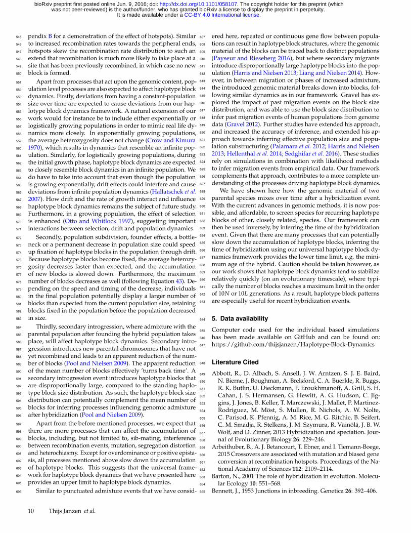
B. Hotspots812

Non-uniform recombination rates might also manifest them-813

selves as a result of recombination hotspots. Recombination814

hotspots delineate areas in the genome that recombine more of-815

ten than other areas, and are well documented in many different816

species (Gerton et al. 2000; Myers et al. 2005; Mackiewicz et al.817

2013; Singhal et al. 2015; Arbeithuber et al. 2015; Smagulova et al.818

2011). The density of recombination hotspots is generally large819

with hotspots occuring every 200kb. Depending on the size of820

the chromosome, this results in a total number of hotspots per821

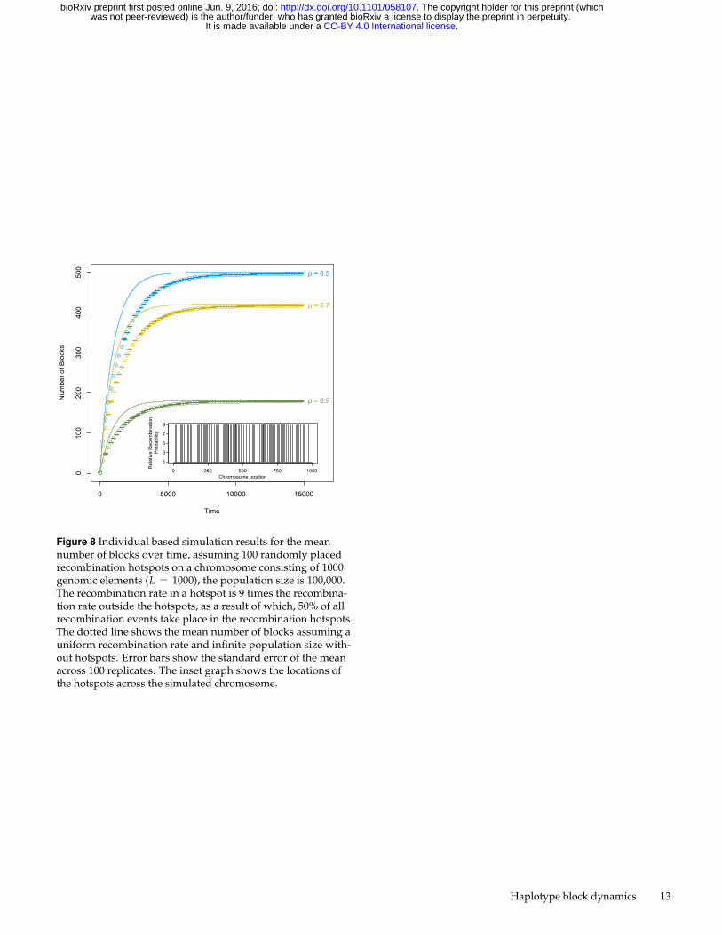
chromosome between 300 and 1200. To demonstrate the effect of822

hotspots on haplotype block dynamics, we model a chromosome823

consisting of 1000 genomic elements (L = 1000). We assume824

100 recombination hotspots scattered randomly across the chro-825

mosome, where the recombination rate is 9 times the normal826

recombination rate, such that 50% of all recombination events827

take place in recombination hotspots (McVean et al. 2004). The828

locations of the recombination hotspots were determined apriori829

and kept constant across replicates and parameter settings. We830

find that recombination hotspots slow down the formation of831

haplotype blocks (Figure 8), as recombination is more likely to832

take place at a site that has previously recombined, compared833

to a uniform recombination rate. The maximum number of834

haplotype blocks remains unaffected.835

0 500 1000 1500 2000

05

1015

2025

Time

Num

ber o

f Blo

cks

p = 0.5

p = 0.7

p = 0.9

0 10 20 30 40 50

0246810

Rel

ativ

e R

ecom

bina

tion

Pro

babi

lity

Chromosome position

Figure 7 Individual based simulation results for the meannumber of blocks over time, assuming an exponential recombi-nation rate distribution with a 10 times higher recombinationrate towards the peripheral ends of the chromosome. The re-combination rate of site i along a chromosome of length L, as-suming the centromere is located at position L/2 is then given

by: P(R, i) = exp(

log(10) |2i−L|L

). The population size N is

100,000 individuals and the number of chromosome elementsL is 50. The solid line shows the mean number of blocks as-suming a uniform recombination rate and infinite populationsize. Error bars show the standard error of the mean across100 replicates. The inset graph shows the recombination rateacross the chromosome relative to the recombination rate atthe centromere, with the dotted line indicating the position ofthe centromere (at L/2).




http://dx.doi.org/10.1101/058107


0 5000 10000 15000

0100

200

300

400

500

Time

Num

ber o

f Blo

cks

p = 0.5

p = 0.7

p = 0.9

0 250 500 750 1000

1

3

5

7

9

Rel

ativ

e R

ecom

bina

tion

Pro

babi

lity

Chromosome position

Figure 8 Individual based simulation results for the meannumber of blocks over time, assuming 100 randomly placedrecombination hotspots on a chromosome consisting of 1000genomic elements (L = 1000), the population size is 100,000.The recombination rate in a hotspot is 9 times the recombina-tion rate outside the hotspots, as a result of which, 50% of allrecombination events take place in the recombination hotspots.The dotted line shows the mean number of blocks assuming auniform recombination rate and infinite population size with-out hotspots. Error bars show the standard error of the meanacross 100 replicates. The inset graph shows the locations ofthe hotspots across the simulated chromosome.




http://dx.doi.org/10.1101/058107


Documents

Haplotype block dynamics in hybrid populations - bioRxiv.org · Haplotype block dynamics in hybrid populations ... doi: 10.1534/genetics.XXX.XXXXXX Manuscript compiled: Thursday 9th