19. BIG-BANG COSMOLOGY - Particle Data Grouppdg.lbl.gov/2005/reviews/bigbangrpp.pdf · 19.Big-Bangcosmology 1 19. BIG-BANG COSMOLOGY Written July 2001 by K.A. Olive (University of

19. Big-Bang cosmology 1

19. BIG-BANG COSMOLOGYWritten July 2001 by K.A. Olive (University of Minnesota) and J.A. Peacock (Universityof Edinburgh). Revised September 2005.

19.1. Introduction to Standard Big-Bang Model

The observed expansion of the Universe [1,2,3] is a natural (almost inevitable) result ofany homogeneous and isotropic cosmological model based on general relativity. However,by itself, the Hubble expansion does not provide sufficient evidence for what we generallyrefer to as the Big-Bang model of cosmology. While general relativity is in principlecapable of describing the cosmology of any given distribution of matter, it is extremelyfortunate that our Universe appears to be homogeneous and isotropic on large scales.Together, homogeneity and isotropy allow us to extend the Copernican Principle to theCosmological Principle, stating that all spatial positions in the Universe are essentiallyequivalent.

The formulation of the Big-Bang model began in the 1940s with the work of GeorgeGamow and his collaborators, Alpher and Herman. In order to account for the possibilitythat the abundances of the elements had a cosmological origin, they proposed thatthe early Universe which was once very hot and dense (enough so as to allow for thenucleosynthetic processing of hydrogen), and has expanded and cooled to its presentstate [4,5]. In 1948, Alpher and Herman predicted that a direct consequence of thismodel is the presence of a relic background radiation with a temperature of order a fewK [6,7]. Of course this radiation was observed 16 years later as the microwave backgroundradiation [8]. Indeed, it was the observation of the 3 K background radiation that singledout the Big-Bang model as the prime candidate to describe our Universe. Subsequentwork on Big-Bang nucleosynthesis further confirmed the necessity of our hot and densepast. (See the review on BBN—Sec. 20 of this Review for a detailed discussion of BBN.)These relativistic cosmological models face severe problems with their initial conditions,to which the best modern solution is inflationary cosmology, discussed in Sec. 19.3.5. Ifcorrect, these ideas would strictly render the term ‘Big Bang’ redundant, since it wasfirst coined by Hoyle to represent a criticism of the lack of understanding of the initialconditions.

19.1.1. The Robertson-Walker Universe:The observed homogeneity and isotropy enable us to describe the overall geometry

and evolution of the Universe in terms of two cosmological parameters accounting forthe spatial curvature and the overall expansion (or contraction) of the Universe. Thesetwo quantities appear in the most general expression for a space-time metric which has a(3D) maximally symmetric subspace of a 4D space-time, known as the Robertson-Walkermetric:

ds2 = dt2 −R2(t)[

dr2

1 − kr2+ r2 (dθ2 + sin2 θ dφ2)

]. (19.1)

Note that we adopt c = 1 throughout. By rescaling the radial coordinate, we can choosethe curvature constant k to take only the discrete values +1, −1, or 0 correspondingto closed, open, or spatially flat geometries. In this case, it is often more convenient tore-express the metric as

CITATION: S. Eidelman et al., Physics Letters B592, 1 (2004)

available on the PDG WWW pages (URL: http://pdg.lbl.gov/) December 20, 2005 11:23

2 19. Big-Bang cosmology

ds2 = dt2 −R2(t)[dχ2 + S2

k(χ) (dθ2 + sin2 θ dφ2)], (19.2)

where the function Sk(χ) is (sinχ, χ, sinhχ) for k = (+1, 0,−1). The coordinate r (inEq. (19.1)) and the ‘angle’ χ (in Eq. (19.2)) are both dimensionless; the dimensions arecarried by R(t), which is the cosmological scale factor which determines proper distancesin terms of the comoving coordinates. A common alternative is to define a dimensionlessscale factor, a(t) = R(t)/R0, where R0 ≡ R(t0) is R at the present epoch. It is alsosometimes convenient to define a dimensionless or conformal time coordinate, η, bydη = dt/R(t). Along constant spatial sections, the proper time is defined by the timecoordinate, t. Similarly, for dt = dθ = dφ = 0, the proper distance is given by R(t)χ. Forstandard texts on cosmological models see e.g., Refs. [9–14].

19.1.2. The redshift:The cosmological redshift is a direct consequence of the Hubble expansion, determined

by R(t). A local observer detecting light from a distant emitter sees a redshift infrequency. We can define the redshift as

z ≡ ν1 − ν2ν2

' v12c

, (19.3)

where ν1 is the frequency of the emitted light, ν2 is the observed frequency and v12is the relative velocity between the emitter and the observer. While the definition,z = (ν1 − ν2)/ν2 is valid on all distance scales, relating the redshift to the relative velocityin this simple way is only true on small scales (i.e., less than cosmological scales) suchthat the expansion velocity is non-relativistic. For light signals, we can use the metricgiven by Eq. (19.1) and ds2 = 0 to write

v12c

= R δr =R

Rδt =

δR

R=R2 −R1

R1, (19.4)

where δr(δt) is the radial coordinate (temporal) separation between the emitter andobserver. Thus, we obtain the simple relation between the redshift and the scale factor

1 + z =ν1ν2

=R2

R1. (19.5)

This result does not depend on the non-relativistic approximation.

December 20, 2005 11:23


19.1.3. The Friedmann-Lemaıtre equations of motion:The cosmological equations of motion are derived from Einstein’s equations

Rµν − 12gµνR = 8πGNTµν + Λgµν . (19.6)

Gliner [15] and Zeldovich [16] seem to have pioneered the modern view, in which the Λterm is taken to the rhs and interpreted as particle-physics processes yielding an effectiveenergy–momentum tensor Tµν for the vacuum of Λgµν/8πGN. It is common to assumethat the matter content of the Universe is a perfect fluid, for which

Tµν = −pgµν + (p+ ρ)uµuν , (19.7)

where gµν is the space-time metric described by Eq. (19.1), p is the isotropic pressure, ρis the energy density and u = (1, 0, 0, 0) is the velocity vector for the isotropic fluid inco-moving coordinates. With the perfect fluid source, Einstein’s equations lead to theFriedmann-Lemaıtre equations

H2 ≡(R

R

)2

=8π GN ρ

3− k

R2+

Λ3, (19.8)

andR

R=

Λ3− 4πGN

3(ρ+ 3p) , (19.9)

where H(t) is the Hubble parameter and Λ is the cosmological constant. The first of theseis sometimes called the Friedmann equation. Energy conservation via Tµν

;µ = 0, leads to athird useful equation [which can also be derived from Eq. (19.8) and Eq. (19.9)]

ρ = −3H (ρ+ p) . (19.10)

Eq. (19.10) can also be simply derived as a consequence of the first law of thermodynamics.Eq. (19.8) has a simple classical mechanical analog if we neglect (for the moment)

the cosmological term Λ. By interpreting −k/R2 as a “total energy”, then we see thatthe evolution of the Universe is governed by a competition between the potential energy,8πGNρ/3 and the kinetic term (R/R)2. For Λ = 0, it is clear that the Universe mustbe expanding or contracting (except at the turning point prior to collapse in a closedUniverse). The ultimate fate of the Universe is determined by the curvature constantk. For k = +1, the Universe will recollapse in a finite time, whereas for k = 0,−1, theUniverse will expand indefinitely. These simple conclusions can be altered when Λ 6= 0 ormore generally with some component with (ρ+ 3p) < 0.

December 20, 2005 11:23


19.1.4. Definition of cosmological parameters:In addition to the Hubble parameter, it is useful to define several other measurable

cosmological parameters. The Friedmann equation can be used to define a critical densitysuch that k = 0 when Λ = 0,

ρc ≡3H2

8πGN= 1.88 × 10−26 h2 kg m−3

= 1.05 × 10−5 h2 GeV cm−3 ,

(19.11)

where the scaled Hubble parameter, h, is defined by

H ≡ 100h km s−1 Mpc−1

⇒ H−1 = 9.78h−1 Gyr

= 2998h−1 Mpc .

(19.12)

The cosmological density parameter Ωtot is defined as the energy density relative to thecritical density,

Ωtot = ρ/ρc . (19.13)

Note that one can now rewrite the Friedmann equation as

k/R2 = H2(Ωtot − 1) , (19.14)

From Eq. (19.14), one can see that when Ωtot > 1, k = +1 and the Universe is closed,when Ωtot < 1, k = −1 and the Universe is open, and when Ωtot = 1, k = 0, and theUniverse is spatially flat.

It is often necessary to distinguish different contributions to the density. It is thereforeconvenient to define present-day density parameters for pressureless matter (Ωm) andrelativistic particles (Ωr), plus the quantity ΩΛ = Λ/3H2. In more general models, wemay wish to drop the assumption that the vacuum energy density is constant, and wetherefore denote the present-day density parameter of the vacuum by Ωv. The Friedmannequation then becomes

k/R20 = H2

0 (Ωm + Ωr + Ωv − 1) , (19.15)

where the subscript 0 indicates present-day values. Thus, it is the sum of the densitiesin matter, relativistic particles and vacuum that determines the overall sign of thecurvature. Note that the quantity −k/R2

0H20 is sometimes referred to as Ωk. This usage

is unfortunate: it encourages one to think of curvature as a contribution to the energydensity of the Universe, which is not correct.

December 20, 2005 11:23


19.1.5. Standard Model solutions:Much of the history of the Universe in the standard Big-Bang model can be easily

described by assuming that either matter or radiation dominates the total energy density.During inflation or perhaps even today if we are living in an accelerating Universe,domination by a cosmological constant or some other form of dark energy should beconsidered. In the following, we shall delineate the solutions to the Friedmann equationwhen a single component dominates the energy density. Each component is distinguishedby an equation of state parameter w = p/ρ.

19.1.5.1. Solutions for a general equation of state:Let us first assume a general equation of state parameter for a single component, w

which is constant. In this case, Eq. (19.10) can be written as ρ = −3(1 + w)ρR/R and iseasily integrated to yield

ρ ∝ R−3(1+w) . (19.16)

Note that at early times when R is small, the less singular curvature term k/R2 inthe Friedmann equation can be neglected so long as w > −1/3. Curvature dominationoccurs at rather late times (if a cosmological constant term does not dominate sooner).For w 6= −1, one can insert this result into the Friedmann equation Eq. (19.8) and ifone neglects the curvature and cosmological constant terms, it is easy to integrate theequation to obtain,

R(t) ∝ t2/[3(1+w)] . (19.17)

19.1.5.2. A Radiation-dominated Universe:In the early hot and dense Universe, it is appropriate to assume an equation of state

corresponding to a gas of radiation (or relativistic particles) for which w = 1/3. In thiscase, Eq. (19.16) becomes ρ ∝ R−4. The “extra” factor of 1/R is due to the cosmologicalredshift; not only is the number density of particles in the radiation background decreasingas R−3 since volume scales as R3, but in addition, each particle’s energy is decreasing asE ∝ ν ∝ R−1. Similarly, one can substitute w = 1/3 into Eq. (19.17) to obtain

R(t) ∝ t1/2 ; H = 1/2t . (19.18)

19.1.5.3. A Matter-dominated Universe:At relatively late times, non-relativistic matter eventually dominates the energy

density over radiation (see Sec. 19.3.8). A pressureless gas (w = 0) leads to the expecteddependence ρ ∝ R−3 from Eq. (19.16) and, if k = 0, we get

R(t) ∝ t2/3 ; H = 2/3t . (19.19)

December 20, 2005 11:23


19.1.5.4. A Universe dominated by vacuum energy:If there is a dominant source of vacuum energy, V0, it would act as a cosmological

constant with Λ = 8πGNV0 and equation of state w = −1. In this case, the solution tothe Friedmann equation is particularly simple and leads to an exponential expansion ofthe Universe

R(t) ∝ e√

Λ/3t . (19.20)

A key parameter is the equation of state of the vacuum, w ≡ p/ρ: this need not bethe w = −1 of Λ, and may not even be constant [17,18,19]. It is now common to use wto stand for this vacuum equation of state, rather than of any other constituent of theUniverse, and we use the symbol in this sense hereafter. We generally assume w to beindependent of time, and where results relating to the vacuum are quoted without anexplicit w dependence, we have adopted w = −1.

The presence of vacuum energy can dramatically alter the fate of the Universe.For example, if Λ < 0, the Universe will eventually recollapse independent of the signof k. For large values of Λ (larger than the Einstein static value needed to halt anycosmological expansion or contraction), even a closed Universe will expand forever. Oneway to quantify this is the deceleration parameter, q0, defined as

q0 = − RR

R2

∣∣∣∣∣0

=12Ωm + Ωr +

(1 + 3w)2

Ωv . (19.21)

This equation shows us that w < −1/3 for the vacuum may lead to an acceleratingexpansion. Astonishingly, it appears that such an effect has been observed in theSupernova Hubble diagram [20–23] (see Fig. 19.1 below); current data indicate thatvacuum energy is indeed the largest contributor to the cosmological density budget, withΩv = 0.72 ± 0.05 and Ωm = 0.28 ± 0.05 if k = 0 is assumed [23].

The nature of this dominant term is presently uncertain, but much effort is beinginvested in dynamical models (e.g., rolling scalar fields), under the catch-all heading of“quintessence.”

19.2. Introduction to Observational Cosmology

19.2.1. Fluxes, luminosities, and distances:The key quantities for observational cosmology can be deduced quite directly from the

metric.(1) The proper transverse size of an object seen by us to subtend an angle dψ is its

comoving size dψ Sk(χ) times the scale factor at the time of emission:

d` = dψ R0Sk(χ)/(1 + z) . (19.22)

(2) The apparent flux density of an object is deduced by allowing its photons to flowthrough a sphere of current radius R0Sk(χ); but photon energies and arrival rates areredshifted, and the bandwidth dν is reduced. The observed photons at frequency ν0 were

December 20, 2005 11:23


emitted at frequency ν0(1 + z), so the flux density is the luminosity at this frequency,divided by the total area, divided by 1 + z:

Sν(ν0) =Lν([1 + z]ν0)

4πR20S

2k(χ)(1 + z)

. (19.23)

These relations lead to the following common definitions:

angular-diameter distance: DA = (1 + z)−1R0Sk(χ)luminosity distance: DL = (1 + z) R0Sk(χ)

(19.24)

These distance-redshift relations are expressed in terms of observables by using theequation of a null radial geodesic (R(t)dχ = dt) plus the Friedmann equation:

R0dχ =1

H(z)dz =

1H0

[(1 − Ωm − Ωv − Ωr)(1 + z)2

+ Ωv(1 + z)3+3w + Ωm(1 + z)3 + Ωr(1 + z)4]−1/2

dz .

(19.25)

The main scale for the distance here is the Hubble length, 1/H0.The flux density is the product of the specific intensity Iν and the solid angle dΩ

subtended by the source: Sν = Iν dΩ. Combining the angular size and flux-densityrelations thus gives the relativistic version of surface-brightness conservation:

Iν(ν0) =Bν([1 + z]ν0)

(1 + z)3, (19.26)

where Bν is surface brightness (luminosity emitted into unit solid angle per unit areaof source). We can integrate over ν0 to obtain the corresponding total or bolometricformula:

Itot =Btot

(1 + z)4. (19.27)

This cosmology-independent form expresses Liouville’s Theorem: photon phase-spacedensity is conserved along rays.

19.2.2. Distance data and geometrical tests of cosmology:In order to confront these theoretical predictions with data, we have to bridge the

divide between two extremes. Nearby objects may have their distances measured quiteeasily, but their radial velocities are dominated by deviations from the ideal Hubbleflow, which typically have a magnitude of several hundred km s−1. On the other hand,objects at redshifts z >∼ 0.01 will have observed recessional velocities that differ fromtheir ideal values by <∼ 10%, but absolute distances are much harder to supply in thiscase. The traditional solution to this problem is the construction of the distance ladder:an interlocking set of methods for obtaining relative distances between various classes ofobject, which begins with absolute distances at the 10 to 100 pc level and terminates with

December 20, 2005 11:23


galaxies at significant redshifts. This is reviewed in the review on Global cosmologicalparameters—Sec. 21 of this Review.

By far the most exciting development in this area has been the use of typeIa Supernovae (SNe), which now allow measurement of relative distances with 5%precision. In combination with Cepheid data from the HST key project on the distancescale, SNe results are the dominant contributor to the best modern value for H0:72 km s−1Mpc−1 ± 10% [24]. Better still, the analysis of high-z SNe has allowed the firstmeaningful test of cosmological geometry to be carried out: as shown in Fig. 19.1 andFig. 19.2, a combination of supernova data and measurements of microwave-backgroundanisotropies strongly favors a k = 0 model dominated by vacuum energy. (See the reviewon Global cosmological parameters—Sec. 21 of this Review for a more comprehensivereview of Hubble parameter determinations.)

19.2.3. Age of the Universe:The most striking conclusion of relativistic cosmology is that the Universe has not

existed forever. The dynamical result for the age of the Universe may be written as

H0t0 =∫ ∞

0

dz

(1 + z)H(z)

=∫ ∞

0

dz

(1 + z) [(1 + z)2(1 + Ωmz) − z(2 + z)Ωv ]1/2, (19.28)

where we have neglected Ωr and chosen w = −1. Over the range of interest (0.1 <∼ Ωm<∼ 1,

|Ωv| <∼ 1), this exact answer may be approximated to a few % accuracy by

H0t0 ' 23 (0.7Ωm + 0.3 − 0.3Ωv)−0.3 . (19.29)

For the special case that Ωm + Ωv = 1, the integral in Eq. (19.28) can be expressedanalytically as

H0t0 =2

3√

Ωvln

1 +√

Ωv√1 − Ωv

(Ωm < 1) . (19.30)

The most accurate means of obtaining ages for astronomical objects is based on thenatural clocks provided by radioactive decay. The use of these clocks is complicated bya lack of knowledge of the initial conditions of the decay. In the Solar System, chemicalfractionation of different elements helps pin down a precise age for the pre-Solar nebulaof 4.6 Gyr, but for stars it is necessary to attempt an a priori calculation of the relativeabundances of nuclei that result from supernova explosions. In this way, a lower limit forthe age of stars in the local part of the Milky Way of about 11 Gyr is obtained [25].

The other major means of obtaining cosmological age estimates is based on the theoryof stellar evolution. In principle, the main-sequence turnoff point in the color-magnitudediagram of a globular cluster should yield a reliable age. However, these have beencontroversial owing to theoretical uncertainties in the evolution model, as well as

December 20, 2005 11:23


Figure 19.1: The type Ia supernova Hubble diagram [20–22]. The first panel showsthat for z 1 the large-scale Hubble flow is indeed linear and uniform; the secondpanel shows an expanded scale, with the linear trend divided out, and with theredshift range extended to show how the Hubble law becomes nonlinear. (Ωr = 0 isassumed.) Comparison with the prediction of Friedmann-Lemaitre models appearsto favor a vacuum-dominated Universe.

observational uncertainties in the distance, dust extinction and metallicity of clusters.The present consensus favors ages for the oldest clusters of about 12 Gyr [26,27].

December 20, 2005 11:23


These methods are all consistent with the age deduced from studies of structureformation, using the microwave background and large-scale structure: t0 = 13.7± 0.2 Gyr[28], where the extra accuracy comes at the price of assuming the Cold Dark Mattermodel to be true.

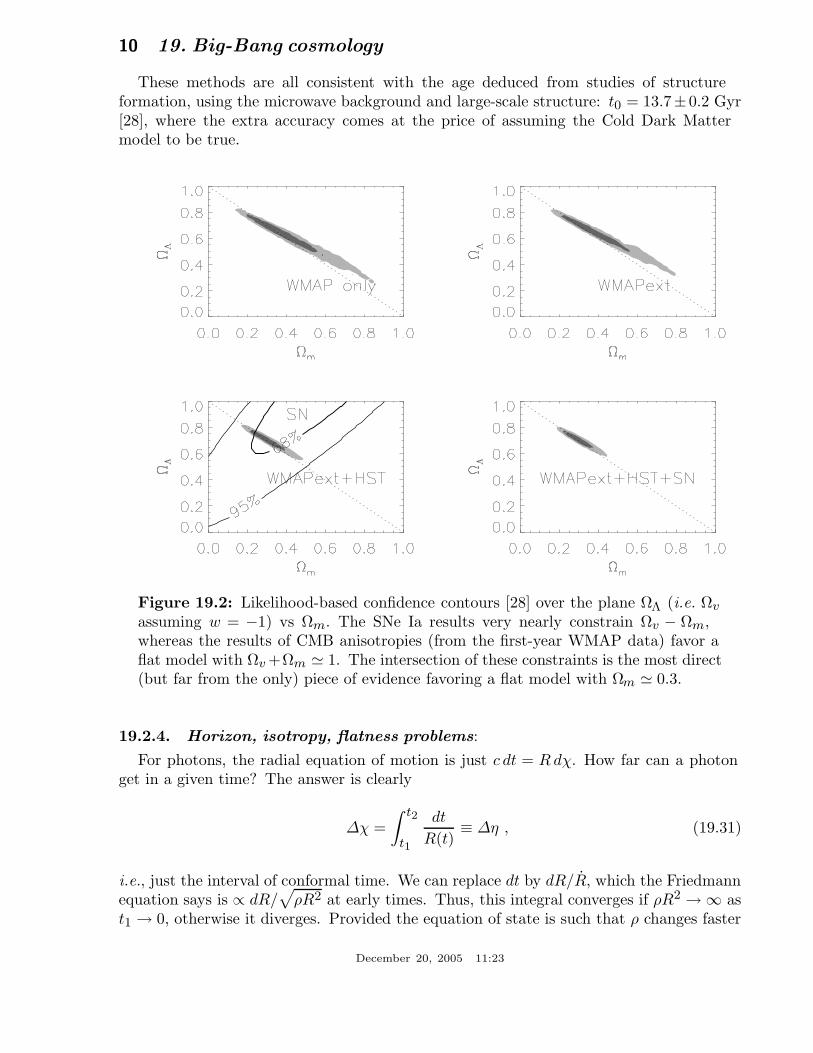
Figure 19.2: Likelihood-based confidence contours [28] over the plane ΩΛ (i.e. Ωv

assuming w = −1) vs Ωm. The SNe Ia results very nearly constrain Ωv − Ωm,whereas the results of CMB anisotropies (from the first-year WMAP data) favor aflat model with Ωv +Ωm ' 1. The intersection of these constraints is the most direct(but far from the only) piece of evidence favoring a flat model with Ωm ' 0.3.

19.2.4. Horizon, isotropy, flatness problems:For photons, the radial equation of motion is just c dt = Rdχ. How far can a photon

get in a given time? The answer is clearly

∆χ =∫ t2

t1

dt

R(t)≡ ∆η , (19.31)

i.e., just the interval of conformal time. We can replace dt by dR/R, which the Friedmannequation says is ∝ dR/

√ρR2 at early times. Thus, this integral converges if ρR2 → ∞ as

t1 → 0, otherwise it diverges. Provided the equation of state is such that ρ changes faster

December 20, 2005 11:23


than R−2, light signals can only propagate a finite distance between the Big Bang andthe present; there is then said to be a particle horizon. Such a horizon therefore existsin conventional Big-Bang models, which are dominated by radiation (ρ ∝ R−4) at earlytimes.

At late times, the integral for the horizon is largely determined by the matter-dominatedphase, for which

DH = R0 χH≡ R0

∫ t(z)

0

dt

R(t)' 6000√

Ωzh−1 Mpc (z 1) . (19.32)

The horizon at the time of formation of the microwave background (‘last scattering’:z ' 1100) was thus of order 100 Mpc in size, subtending an angle of about 1. Why thenare the large number of causally disconnected regions we see on the microwave sky allat the same temperature? The Universe is very nearly isotropic and homogeneous, eventhough the initial conditions appear not to permit such a state to be constructed.

A related problem is that the Ω = 1 Universe is unstable:

Ω(a) − 1 =Ω − 1

1 − Ω + Ωva2 + Ωma−1 + Ωra−2, (19.33)

where Ω with no subscript is the total density parameter, and a(t) = R(t)/R0. Thisrequires Ω(t) to be unity to arbitrary precision as the initial time tends to zero; a universeof non-zero curvature today requires very finely tuned initial conditions.

19.3. The Hot Thermal Universe

19.3.1. Thermodynamics of the early Universe:As alluded to above, we expect that much of the early Universe can be described by

a radiation-dominated equation of state. In addition, through much of the radiation-dominated period, thermal equilibrium is established by the rapid rate of particleinteractions relative to the expansion rate of the Universe (see Sec. 19.3.3 below). Inequilibrium, it is straightforward to compute the thermodynamic quantities, ρ, p, andthe entropy density, s. In general, the energy density for a given particle type i can bewritten as

ρi =∫Ei dnqi , (19.34)

with the density of states given by

dnqi =gi

2π2

(exp[(Eqi − µi)/Ti] ± 1

)−1q2i dqi , (19.35)

where gi counts the number of degrees of freedom for particle type i, E2qi

= m2i + q2i ,

µi is the chemical potential, and the ± corresponds to either Fermi or Bose statistics.Similarly, we can define the pressure of a perfect gas as

pi =13

∫q2iEi

dnqi . (19.36)

December 20, 2005 11:23


The number density of species i is simply

ni =∫dnqi , (19.37)

and the entropy density is

si =ρi + pi − µini

Ti, (19.38)

In the Standard Model, a chemical potential is often associated with baryon number,and since the net baryon density relative to the photon density is known to be verysmall (of order 10−10), we can neglect any such chemical potential when computing totalthermodynamic quantities.

For photons, we can compute all of the thermodynamic quantities rather easily. Takinggi = 2 for the 2 photon polarization states, we have

ργ =π2

15T 4 ; pγ =

13ργ ; sγ =

4ργ

3T; nγ =

2ζ(3)π2

T 3 , (19.39)

with 2ζ(3)/π2 ' 0.2436. Note that Eq. (19.10) can be converted into an equation forentropy conservation. Recognizing that p = sT , Eq. (19.10) becomes

d(sR3)/dt = 0 . (19.40)

For radiation, this corresponds to the relationship between expansion and cooling,T ∝ R−1 in an adiabatically expanding Universe. Note also that both s and nγ scale asT 3.

19.3.2. Radiation content of the Early Universe:

At the very high temperatures associated with the early Universe, massive particlesare pair produced, and are part of the thermal bath. If for a given particle species iwe have T mi, then we can neglect the mass in Eq. (19.34) to Eq. (19.38), and thethermodynamic quantities are easily computed as in Eq. (19.39). In general, we canapproximate the energy density (at high temperatures) by including only those particleswith mi T . In this case, we have

ρ =

(∑B

gB +78

∑F

gF

)π2

30T 4 ≡ π2

30N(T )T 4 , (19.41)

where gB(F ) is the number of degrees of freedom of each boson (fermion) and the sumruns over all boson and fermion states with m T . The factor of 7/8 is due to thedifference between the Fermi and Bose integrals. Eq. (19.41) defines the effective numberof degrees of freedom, N(T ), by taking into account new particle degrees of freedom asthe temperature is raised. This quantity is plotted in Fig. 19.3 [29].

December 20, 2005 11:23


Temperature New Particles 4N(T )T < me γ’s + ν’s 29me < T < mµ e± 43mµ < T < mπ µ± 57mπ < T < T

†c π’s 69

Tc < T < mstrange π’s + u, u, d, d + gluons 205ms < T < mcharm s, s 247mc < T < mτ c, c 289mτ < T < mbottom τ± 303mb < T < mW,Z b, b 345mW,Z < T < mHiggs W±, Z 381mH < T < mtop H0 385mt < T t, t 427

†Tc corresponds to the confinement-deconfinement transition between quarks and hadrons.

The value of N(T ) at any given temperature depends on the particle physics model.In the standard SU(3)× SU(2)×U(1) model, we can specify N(T ) up to temperatures ofO(100) GeV. The change in N (ignoring mass effects) can be seen in the following table.

At higher temperatures, N(T ) will be model dependent. For example, in the minimalSU(5) model, one needs to add 24 states to N(T ) for the X and Y gauge bosons, another24 from the adjoint Higgs, and another 6 (in addition to the 4 already counted in W±, Z,and H) from the 5 of Higgs. Hence for T > mX in minimal SU(5), N(T ) = 160.75. In asupersymmetric model this would at least double, with some changes possibly necessaryin the table if the lightest supersymmetric particle has a mass below mt.

In the radiation-dominated epoch, Eq. (19.10) can be integrated (neglecting theT -dependence of N) giving us a relationship between the age of the Universe and itstemperature

t =(

9032π3GNN(T )

)1/2

T−2 , (19.42)

Put into a more convenient form

t T 2MeV = 2.4[N(T )]−1/2 , (19.43)

where t is measured in seconds and TMeV in units of MeV.

19.3.3. Neutrinos and equilibrium:

Due to the expansion of the Universe, certain rates may be too slow to either establishor maintain equilibrium. Quantitatively, for each particle i, as a minimal condition forequilibrium, we will require that some rate Γi involving that type be larger than theexpansion rate of the Universe or

Γi > H . (19.44)

December 20, 2005 11:23


0

20

40

60

80

100

1.6 1.8 2.0 2.2 2.4 2.6 2.8 3.0 3.2 3.4 3.6 3.8 4.0

N(T)

Log(T/MeV)Figure 19.3: The effective numbers of relativistic degrees of freedom as a functionof temperature. The sharp drop corresponds to the quark-hadron transition. Thesolid curve assume a QCD scale of 150 MeV, while the dashed curve assumes 450MeV.

Recalling that the age of the Universe is determined by H−1, this condition is equivalentto requiring that on average, at least one interaction has occurred over the lifetime of theUniverse.

A good example for a process which goes in and out of equilibrium is the weakinteractions of neutrinos. On dimensional grounds, one can estimate the thermallyaveraged scattering cross section

〈σv〉 ∼ O(10−2)T 2/m4W (19.45)

for T <∼ mW. Recalling that the number density of leptons is n ∝ T 3, we can comparethe weak interaction rate, Γ ∼ n〈σv〉, with the expansion rate,

H =(

8πGNρ

3

)1/2

=(

8π3

90N(T )

)1/2

T 2/MP

∼ 1.66N(T )1/2T 2/MP.

(19.46)

The Planck mass MP = G−1/2N = 1.22 × 1019 GeV.

Neutrinos will be in equilibrium when Γwk > H or

T > (500m4W/MP)1/3 ∼ 1 MeV . (19.47)

December 20, 2005 11:23


The temperature at which these rates are equal is commonly referred to as the neutrinodecoupling or freeze-out temperature and is defined by Γ(Td) = H(Td).

At very high temperatures, the Universe is too young for equilibrium to have beenestablished. For T mW, we should write 〈σv〉 ∼ O(10−2)/T 2, so that Γ ∼ 10−2T .Thus at temperatures T >∼ 10−2MP/

√N , equilibrium will not have been established.

For T < Td, neutrinos drop out of equilibrium. The Universe becomes transparent toneutrinos and their momenta simply redshift with the cosmic expansion. The effectiveneutrino temperature will simply fall with T ∼ 1/R.

Soon after decoupling, e± pairs in the thermal background begin to annihilate (whenT <∼ me). Because the neutrinos are decoupled, the energy released due to annihilationheats up the photon background relative to the neutrinos. The change in the photontemperature can be easily computed from entropy conservation. The neutrino entropymust be conserved separately from the entropy of interacting particles. A straightforwardcomputation yields

Tν = (4/11)1/3 Tγ ' 1.9 K . (19.48)

Today, the total entropy density is therefore given by

s =43π2

30

(2 +

214

(Tν/Tγ)3)T 3

γ =43π2

30

(2 +

2111

)T 3

γ = 7.04nγ . (19.49)

Similarly, the total relativistic energy density today is given by

ρr =π2

30

[2 +

214

(Tν/Tγ)4]T 4

γ ' 1.68ργ . (19.50)

In practice, a small correction is needed to this, since neutrinos are not totallydecoupled at e± annihilation: the effective number of massless neutrino species is 3.04,rather than 3 [30].

This expression ignores neutrino rest masses, but current oscillation data requireat least one neutrino eigenstate to have a mass exceeding 0.05 eV. In this minimalcase, Ωνh

2 = 5 × 10−4, so the neutrino contribution to the matter budget would benegligibly small (which is our normal assumption). However, a nearly degenerate patternof mass eigenstates could allow larger densities, since oscillation experiments only measuredifferences in m2 values. Note that a 0.05-eV neutrino has kTν = mν at z ' 297, so theabove expression for the total present relativistic density is really only an extrapolation.However, neutrinos are almost certainly relativistic at all epochs where the radiationcontent of the universe is dynamically significant.

December 20, 2005 11:23


19.3.4. Field Theory and Phase transitions:It is very likely that the Universe has undergone one or more phase transitions during

the course of its evolution [31–34]. Our current vacuum state is described by SU(3)c×U(1)em which in the Standard Model is a remnant of an unbroken SU(3)c× SU(2)L×U(1)Y gauge symmetry. Symmetry breaking occurs when a non-singlet gauge field (theHiggs field in the Standard Model) picks up a non-vanishing vacuum expectation value,determined by a scalar potential. For example, a simple (non-gauged) potential describingsymmetry breaking is V (φ) = 1

4λφ4 − 1

2µ2φ2 + V (0). The resulting expectation value is

simply 〈φ〉 = µ/√λ.

In the early Universe, finite temperature radiative corrections typically add termsto the potential of the form φ2T 2. Thus, at very high temperatures, the symmetry isrestored and 〈φ〉 = 0. As the Universe cools, depending on the details of the potential,symmetry breaking will occur via a first order phase transition in which the field tunnelsthrough a potential barrier, or via a second order transition in which the field evolvessmoothly from one state to another (as would be the case for the above examplepotential).

The evolution of scalar fields can have a profound impact on the early Universe. Theequation of motion for a scalar field φ can be derived from the energy-momentum tensor

Tµν = ∂µφ∂νφ− 12gµν∂ρφ∂

ρφ− gµνV (φ) . (19.51)

By associating ρ = T00 and p = R−2(t)Tii we have

ρ =12φ2 +

12R−2(t)(∇φ)2 + V (φ)

p =12φ2 − 1

6R−2(t)(∇φ)2 − V (φ)

(19.52)

and from Eq. (19.10) we can write the equation of motion (by considering a homogeneousregion, we can ignore the gradient terms)

φ+ 3Hφ = −∂V/∂φ . (19.53)

19.3.5. Inflation:In Sec. 19.2.4, we discussed some of the problems associated with the standard

Big-Bang model. However, during a phase transition, our assumptions of an adiabaticallyexpanding universe are generally not valid. If, for example, a phase transition occurredin the early Universe such that the field evolved slowly from the symmetric state to theglobal minimum, the Universe may have been dominated by the vacuum energy densityassociated with the potential near φ ≈ 0. During this period of slow evolution, the energydensity due to radiation will fall below the vacuum energy density, ρ V (0). When thishappens, the expansion rate will be dominated by the constant V(0) and we obtain theexponentially expanding solution given in Eq. (19.20). When the field evolves towards

December 20, 2005 11:23


the global minimum it will begin to oscillate about the minimum, energy will be releasedduring its decay and a hot thermal universe will be restored. If released fast enough, itwill produce radiation at a temperature NTR

4 <∼ V (0). In this reheating process entropyhas been created and the final value of RT is greater than the initial value of RT . Thus,we see that, during a phase transition, the relation RT ∼ constant need not hold true.This is the basis of the inflationary Universe scenario [35–37].

If during the phase transition the value of RT changed by a factor of O(1029), thecosmological problems discussed above would be solved. The observed isotropy would begenerated by the immense expansion; one small causal region could get blown up andhence our entire visible Universe would have been in thermal contact some time in thepast. In addition, the density parameter Ω would have been driven to 1 (with exponentialprecision). Density perturbations will be stretched by the expansion, λ ∼ R(t). Thus itwill appear that λ H−1 or that the perturbations have left the horizon, where in factthe size of the causally connected region is now no longer simply H−1. However, not onlydoes inflation offer an explanation for large scale perturbations, it also offers a source forthe perturbations themselves through quantum fluctuations.

Early models of inflation were based on a first order phase transition of a Grand Unifiedtheory [38]. Although these models led to sufficient exponential expansion, completion ofthe transition through bubble percolation did not occur. Later models of inflation [39,40],also based on Grand Unified symmetry breaking, through second order transitions werealso doomed. While they successfully inflated and reheated, and in fact produced densityperturbations due to quantum fluctuations during the evolution of the scalar field, theypredicted density perturbations many orders of magnitude too large. Most models todayare based on an unknown symmetry breaking involving a new scalar field, the inflaton, φ.

19.3.6. Baryogenesis:The Universe appears to be populated exclusively with matter rather than antimatter.

Indeed antimatter is only detected in accelerators or in cosmic rays. However, thepresence of antimatter in the latter is understood to be the result of collisions of primaryparticles in the interstellar medium. There is in fact strong evidence against primaryforms of antimatter in the Universe. Furthermore, the density of baryons compared tothe density of photons is extremely small, η ∼ 10−10.

The production of a net baryon asymmetry requires baryon number violatinginteractions, C and CP violation and a departure from thermal equilibrium [41]. Thefirst two of these ingredients are expected to be contained in grand unified theories aswell as in the non-perturbative sector of the standard model, the third can be realized inan expanding universe where as we have seen interactions come in and out of equilibrium.

There are several interesting and viable mechanisms for the production of the baryonasymmetry. While, we can not review any of them here in any detail, we mentionsome of the important scenarios. In all cases, all three ingredients listed above areincorporated. One of the first mechanisms was based on the out of equilibrium decayof a massive particle such as a superheavy GUT gauge of Higgs boson [42,43]. A novelmechanism involving the decay of flat directions in supersymmetric models is knownas the Affleck-Dine scenario [44]. Recently, much attention has been focused on the

December 20, 2005 11:23


possibility of generating the baryon asymmetry at the electro-weak scale using thenon-perturbative interactions of sphalerons [45]. Because these interactions conservethe sum of baryon and lepton number, B + L, it is possible to first generate a leptonasymmetry (e.g., by the out-of-equilibrium decay of a superheavy right-handed neutrino),which is converted to a baryon asymmetry at the electro-weak scale [46]. This mechanismis known as lepto-baryogenesis.

19.3.7. Nucleosynthesis:An essential element of the standard cosmological model is Big-Bang nucleosynthesis

(BBN), the theory which predicts the abundances of the light element isotopes D, 3He,4He, and 7Li. Nucleosynthesis takes place at a temperature scale of order 1 MeV. Thenuclear processes lead primarily to 4He, with a primordial mass fraction of about 24%.Lesser amounts of the other light elements are produced: about 10−5 of D and 3He andabout 10−10 of 7Li by number relative to H. The abundances of the light elements dependalmost solely on one key parameter, the baryon-to-photon ratio, η. The nucleosynthesispredictions can be compared with observational determinations of the abundances ofthe light elements. Consistency between theory and observations leads to a conservativerange of

3.4 × 10−10 < η < 6.9 × 10−10 . (19.54)

η is related to the fraction of Ω contained in baryons, Ωb

Ωb = 3.66 × 107η h−2 , (19.55)

or 1010η = 274Ωbh2. The WMAP result [28] for Ωbh

2 of 0.0224 ± 0.0009 translatesinto a value of η = 6.15 ± 0.25. This result can be used to ‘predict’ the light elementabundance which can in turn be compared with observation [47]. The resulting D/Habundance is in excellent agreement with that found in quasar absorption systems. Itis in reasonable agreement with the helium abundance observed in extra-galactic HIIregions (once systematic uncertainties are accounted for) but is in poor agreement withthe Li abundance observed in the atmospheres of halo dwarf stars. (See the review onBBN—Sec. 20 of this Review for a detailed discussion of BBN or references [48,49].)

19.3.8. The transition to a matter-dominated Universe:In the Standard Model, the temperature (or redshift) at which the Universe undergoes

a transition from a radiation dominated to a matter dominated Universe is determined bythe amount of dark matter. Assuming three nearly massless neutrinos, the energy densityin radiation at temperatures T 1 MeV, is given by

ρr =π2

30

[2 +

214

(411

)4/3]T 4 . (19.56)

In the absence of non-baryonic dark matter, the matter density can be written as

ρm = mNη nγ , (19.57)

December 20, 2005 11:23


where mN is the nucleon mass. Recalling that nγ ∝ T 3 [cf. Eq. (19.39)], we can solve forthe temperature or redshift at the matter-radiation equality when ρr = ρm,

Teq = 0.22mN η or (1 + zeq) = 0.22 ηmN

T0, (19.58)

where T0 is the present temperature of the microwave background. For η = 5 × 10−10,this corresponds to a temperature Teq ' 0.1 eV or (1 + zeq) ' 425. A transition this lateis very problematic for structure formation (see Sec. 19.4.5).

The redshift of matter domination can be pushed back significantly if non-baryonicdark matter is present. If instead of Eq. (19.57), we write

ρm = Ωmρc

(T

T0

)3

, (19.59)

we find thatTeq = 0.9

Ωmρc

T 30

or (1 + zeq) = 2.4 × 104Ωmh2 . (19.60)

19.4. The Universe at late times

19.4.1. The CMB:One form of the infamous Olbers’ paradox says that, in Euclidean space, surface

brightness is independent of distance. Every line of sight will terminate on matter thatis hot enough to be ionized and so scatter photons: T >∼ 103 K; the sky should thereforeshine as brightly as the surface of the Sun. The reason the night sky is dark is entirelydue to the expansion, which cools the radiation temperature to 2.73 K. This gives aPlanck function peaking at around 1 mm to produce the microwave background (CMB).

The CMB spectrum is a very accurate match to a Planck function [50]. (See the reviewon CBR–Sec. 23 of this Review.) The COBE estimate of the temperature is [51]

T = 2.725 ± 0.002 K . (19.61)

The lack of any distortion of the Planck spectrum is a strong physical constraint. It isvery difficult to account for in any expanding universe other than one that passes througha hot stage. Alternative schemes for generating the radiation, such as thermalizationof starlight by dust grains, inevitably generate a superposition of temperatures. Whatis required in addition to thermal equilibrium is that T ∝ 1/R, so that radiation fromdifferent parts of space appears identical.

Although it is common to speak of the CMB as originating at “recombination,” amore accurate terminology is the era of “last scattering,” In practice, this takes placeat z ' 1100, almost independently of the main cosmological parameters, at which timethe fractional ionization is very small. This occurred when the age of the Universe wasa few hundred thousand years. (See the review on CBR–Sec. 23 of this Review for a fulldiscussion of the CMB.)

December 20, 2005 11:23


19.4.2. Matter in the Universe:One of the main tasks of cosmology is to measure the density of the Universe, and how

this is divided between dark matter and baryons. The baryons consist partly of stars,with 0.002 <∼ Ω∗ <∼ 0.003 [52] but mainly inhabit the IGM. One powerful way in whichthis can be studied is via the absorption of light from distant luminous objects such asquasars. Even very small amounts of neutral hydrogen can absorb rest-frame UV photons(the Gunn-Peterson effect), and should suppress the continuum by a factor exp(−τ),where

τ '[

nHI(z)(1 + z)

√1 + Ωmz

]/ 10−4.62 hm−3, (19.62)

and this expression applies while the Universe is matter dominated (z >∼ 1 in theΩm = 0.3 Ωv = 0.7 model). It is possible that this general absorption has now been seenat z = 6.2 [53]. In any case, the dominant effect on the spectrum is a ‘forest’ of narrowabsorption lines, which produce a mean τ = 1 in the Lyα forest at about z = 3, and so wehave ΩHI ' 10−5.5h−1. This is such a small number that clearly the IGM is very highlyionized at these redshifts.

The Lyα forest is of great importance in pinning down the abundance of deuterium.Because electrons in deuterium differ in reduced mass by about 1 part in 4000 comparedto Hydrogen, each absorption system in the Lyα forest is accompanied by an offsetdeuterium line. By careful selection of systems with an optimal HI column density, ameasurement of the D/H ratio can be made. This has now been done in 5 quasars,with relatively consistent results [49]. Combining these determinations with the theoryof primordial nucleosynthesis yields a baryon density of Ωbh

2 = 0.021 ± 0.004 (95%confidence). (See also the review on BBN—Sec. 20 of this Review.)

Ionized IGM can also be detected in emission when it is densely clumped, viabremsstrahlung radiation. This generates the spectacular X-ray emission from richclusters of galaxies. Studies of this phenomenon allow us to achieve an accounting of thetotal baryonic material in clusters. Within the central ' 1 Mpc, the masses in stars,X-ray emitting gas and total dark matter can be determined with reasonable accuracy(perhaps 20% rms), and this allows a minimum baryon fraction to be determined [54,55]:

Mbaryons

Mtotal

>∼ 0.009 + (0.066 ± 0.003) h−3/2 . (19.63)

Because clusters are the largest collapsed structures, it is reasonable to take this asapplying to the Universe as a whole. This equation implies a minimum baryon fractionof perhaps 12% (for reasonable h), which is too high for Ωm = 1 if we take Ωbh

2 ' 0.02from nucleosynthesis. This is therefore one of the more robust arguments in favor ofΩm ' 0.3. (See the review on Global cosmological parameters—Sec. 21 of this Review.)This argument is also consistent with the inference on Ωm that can be made fromFig. 19.2.

This method is much more robust than the older classical technique for weighingthe Universe: ‘L ×M/L’. The overall light density of the Universe is reasonably welldetermined from redshift surveys of galaxies, so that a good determination of mass M

December 20, 2005 11:23


and luminosity L for a single object suffices to determine Ωm if the mass-to-light ratio isuniversal.

Galaxy redshift surveys allow us to deduce the galaxy luminosity function, φ, whichis the comoving number density of galaxies; this may be described by the Schechterfunction, which is a power law with an exponential cutoff:

φ = φ∗(L

L∗

)−α

e−L/L∗ dLL∗ (19.64)

The total luminosity density produced by integrating over the distribution is

ρL = φ∗L∗Γ(2 − α) , (19.65)

and this tells us the average mass-to-light ratio needed to close the Universe. Answersvary (principally owing to uncertainties in φ∗). In blue light, the total luminosity densityis ρL = 2±0.2×108 hLMpc−3 [56,57]. The critical density is 2.78×1011 Ωh2MMpc−3,so the critical M/L for closure is

(M/L)crit, B = 1390h± 10% . (19.66)

Dynamical determinations of mass on the largest accessible scales consistently yield blueM/L values of at least 300h, but normally fall short of the closure value [58]. Thiswas a long-standing argument against the Ωm = 1 model, but it was never conclusivebecause the stellar populations in objects such as rich clusters (where the masses can bedetermined) differ systematically from those in other regions.

19.4.3. Gravitational lensing:A robust method for determining masses in cosmology is to use gravitational light

deflection. Most systems can be treated as a geometrically thin gravitational lens, wherethe light bending is assumed to take place only at a single distance. Simple geometrythen determines a mapping between the coordinates in the intrinsic source plane and theobserved image plane:

α(DLθI) =DS

DLS(θI − θS) , (19.67)

where the angles θI, θS and α are in general two-dimensional vectors on the sky. Thedistances DLS etc. are given by an extension of the usual distance-redshift formula:

DLS =R0Sk(χS − χL)

1 + zS. (19.68)

This is the angular-diameter distance for objects on the source plane as perceived by anobserver on the lens.

Solutions of this equation divide into weak lensing, where the mapping between sourceplane and image plane is one-to-one, and strong lensing, in which multiple imaging is

December 20, 2005 11:23


possible. For circularly-symmetric lenses, an on-axis source is multiply imaged into a‘caustic’ ring, whose radius is the Einstein radius:

θE =(

4GMDLS

DLDS

)1/2

=(

M

1011.09M

)1/2 (DLDS/DLS

Gpc

)−1/2

arcsec

(19.69)

The observation of ‘arcs’ (segments of near-perfect Einstein rings) in rich clusters ofgalaxies has thus given very accurate masses for the central parts of clusters—generally ingood agreement with other indicators, such as analysis of X-ray emission from the clusterIGM [59].

19.4.4. Density Fluctuations:The overall properties of the Universe are very close to being homogeneous; and yet

telescopes reveal a wealth of detail on scales varying from single galaxies to large-scalestructures of size exceeding 100 Mpc. The existence of these structures must be tellingus something important about the initial conditions of the Big Bang, and about thephysical processes that have operated subsequently. This motivates the study of thedensity perturbation field, defined as

δ(x) ≡ ρ(x) − 〈ρ〉〈ρ〉 . (19.70)

A critical feature of the δ field is that it inhabits a universe that is isotropic andhomogeneous in its large-scale properties. This suggests that the statistical properties ofδ should also be statistically homogeneous—i.e., it is a stationary random process.

It is often convenient to describe δ as a Fourier superposition:

δ(x) =∑

δke−ik·x . (19.71)

We avoid difficulties with an infinite universe by applying periodic boundary conditionsin a cube of some large volume V . The cross-terms vanish when we compute the variancein the field, which is just a sum over modes of the power spectrum

〈δ2〉 =∑

|δk|2 ≡∑

P (k) . (19.72)

Note that the statistical nature of the fluctuations must be isotropic, so we write P (k)rather than P (k). The 〈. . .〉 average here is a volume average. Cosmological density fieldsare an example of an ergodic process, in which the average over a large volume tends tothe same answer as the average over a statistical ensemble.

The statistical properties of discrete objects sampled from the density field are oftendescribed in terms of N -point correlation functions, which represent the excess probabilityover random for finding one particle in each of N boxes in a given configuration.

December 20, 2005 11:23


For the 2-point case, the correlation function is readily shown to be identical to theautocorrelation function of the δ field: ξ(r) = 〈δ(x)δ(x+ r)〉.

The power spectrum and correlation function are Fourier conjugates, and thus areequivalent descriptions of the density field (similarly, k-space equivalents exist forthe higher-order correlations). It is convenient to take the limit V → ∞ and usek-space integrals, defining a dimensionless power spectrum as ∆2(k) = d〈δ2〉/d lnk =V k3P (k)/2π2:

ξ(r) =∫∆2(k)

sin krkr

d ln k; ∆2(k) =2πk3∫ ∞

0ξ(r)

sin krkr

r2 dr . (19.73)

For many years, an adequate approximation to observational data on galaxies wasξ = (r/r0)−γ , with γ ' 1.8 and r0 ' 5 h−1 Mpc. Modern surveys are now able to probeinto the large-scale linear regime where traces of the curved primordial spectrum can bedetected [60,61].

19.4.5. Formation of cosmological structure:

The simplest model for the generation of cosmological structure is gravitationalinstability acting on some small initial fluctuations (for the origin of which a theorysuch as inflation is required). If the perturbations are adiabatic (i.e., fractionally perturbnumber densities of photons and matter equally), the linear growth law for matterperturbations is simple:

δ ∝a(t)2 (radiation domination; Ωr = 1)a(t) (matter domination; Ωm = 1)

(19.74)

For low density universes, the present-day amplitude is suppressed by a factor g(Ω),where

g(Ω) ' 52Ωm

[Ω4/7

m − Ωv + (1 + Ωm/2)(1 +170

Ωv)]−1

, (19.75)

is an accurate fit for models with matter plus cosmological constant. The alternativeperturbation mode is isocurvature: only the equation of state changes, and the totaldensity is initially unperturbed. These modes perturb the total entropy density, andthus induce additional large-scale CMB anisotropies [62]. Although the character ofperturbations in the simplest inflationary theories are purely adiabatic, correlatedadiabatic and isocurvature modes are predicted in many models; the simplest example isthe curvaton, which is a scalar field that decays to yield a perturbed radiation density. Ifthe matter content already exists at this time, the overall perturbation field will have asignificant isocurvature component. Such a prediction is inconsistent with current CMBdata [63], and most analyses of CMB and LSS data assume the adiabatic case to holdexactly.

Linear evolution preserves the shape of the power spectrum. However, a variety ofprocesses mean that growth actually depends on the matter content:

December 20, 2005 11:23


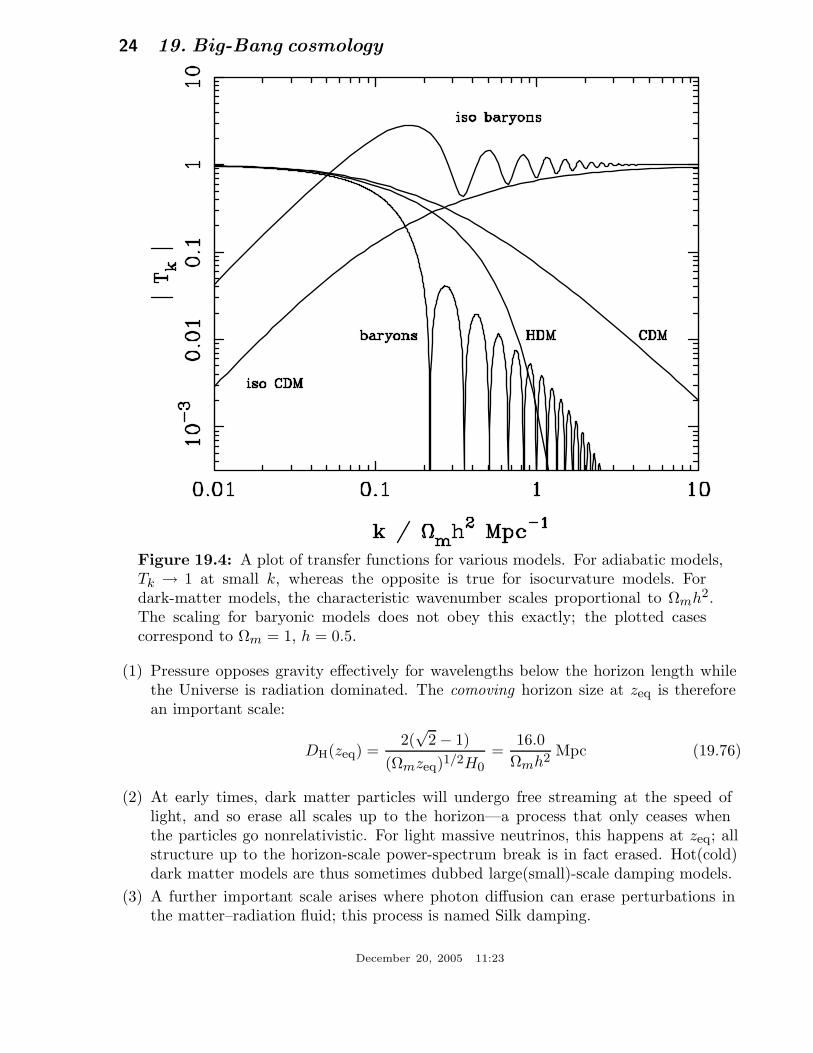
Figure 19.4: A plot of transfer functions for various models. For adiabatic models,Tk → 1 at small k, whereas the opposite is true for isocurvature models. Fordark-matter models, the characteristic wavenumber scales proportional to Ωmh

2.The scaling for baryonic models does not obey this exactly; the plotted casescorrespond to Ωm = 1, h = 0.5.

(1) Pressure opposes gravity effectively for wavelengths below the horizon length whilethe Universe is radiation dominated. The comoving horizon size at zeq is thereforean important scale:

DH(zeq) =2(√

2 − 1)(Ωmzeq)1/2H0

=16.0

Ωmh2Mpc (19.76)

(2) At early times, dark matter particles will undergo free streaming at the speed oflight, and so erase all scales up to the horizon—a process that only ceases whenthe particles go nonrelativistic. For light massive neutrinos, this happens at zeq; allstructure up to the horizon-scale power-spectrum break is in fact erased. Hot(cold)dark matter models are thus sometimes dubbed large(small)-scale damping models.

(3) A further important scale arises where photon diffusion can erase perturbations inthe matter–radiation fluid; this process is named Silk damping.

December 20, 2005 11:23


The overall effect is encapsulated in the transfer function, which gives the ratio ofthe late-time amplitude of a mode to its initial value (see Fig. 19.4). The overall powerspectrum is thus the primordial power-law, times the square of the transfer function:

P (k) ∝ kn T 2k . (19.77)

The most generic power-law index is n = 1: the ‘Zeldovich’ or ‘scale-invariant’ spectrum.Inflationary models tend to predict a small ‘tilt’: |n−1| <∼ 0.03 [13,14]. On the assumptionthat the dark matter is cold, the power spectrum then depends on 5 parameters: n, h,Ωb, Ωcdm (≡ Ωm − Ωb) and an overall amplitude. The latter is often specified as σ8,the linear-theory fractional rms in density when a spherical filter of radius 8h−1 Mpc isapplied in linear theory. This scale can be probed directly via weak gravitational lensing,and also via its effect on the abundance of rich galaxy clusters. The favored value isapproximately [64,65]

σ8 = (0.7 ± 15%) (Ωm/0.3)−0.5 . (19.78)

A direct measure of mass inhomogeneity is valuable, since the galaxies inevitably arebiased with respect to the mass. This means that the fractional fluctuations in galaxynumber, δn/n may differ from the mass fluctuations, δρ/ρ. It is commonly assumed thatthe two fields obey some proportionality on large scales where the fluctuations are small,δn/n = bδρ/ρ, but even this is not guaranteed [66].

The main shape of the transfer function is a break around the horizon scale atzeq, which depends just on Ωmh when wavenumbers are measured in observable units( hMpc−1). In principle, accurate data over a wide range of k could determine both Ωhand n, but in practice there is a strong degeneracy between these. For reasonable baryoncontent, weak oscillations in the transfer function may be visible, giving an alternativemeans of fixing the baryon content. Current data [60,61] favor Ωmh ' 0.20 and a baryonfraction of about 0.15 for n = 1 (see Fig. 19.5). In order to constrain n itself, it isnecessary to examine data on anisotropies in the CMB.

19.4.6. CMB anisotropies:The CMB has a clear dipole anisotropy, of magnitude 1.23 × 10−3. This is interpreted

as being due to the Earth’s motion, which is equivalent to a peculiar velocity for theMilky Way of

vMW ' 600 km s−1 towards (`, b) ' (270, 30) . (19.79)

All higher-order multipole moments of the CMB are however much smaller (of order10−5), and interpreted as signatures of density fluctuations at last scattering (' 1100).To analyze these, the sky is expanded in spherical harmonics as explained in the reviewon CBR–Sec. 23 of this Review. The dimensionless power per ln k or ‘bandpower’ for theCMB is defined as

T 2(`) =`(`+ 1)

2πC` . (19.80)

This function encodes information from the three distinct mechanisms that cause CMBanisotropies:

December 20, 2005 11:23


Figure 19.5: The galaxy power spectrum from the 2dFGRS, shown in dimensionlessform, ∆2(k) ∝ k3P (k). The solid points with error bars show the power estimate.The window function correlates the results at different k values, and also distorts thelarge-scale shape of the power spectrum An approximate correction for the lattereffect has been applied. The solid and dashed lines show various CDM models,all assuming n = 1. For the case with non-negligible baryon content, a big-bangnucleosynthesis value of Ωbh

2 = 0.02 is assumed, together with h = 0.7. A good fitis clearly obtained for Ωmh ' 0.2.

(1) Gravitational (Sachs–Wolfe) perturbations. Photons from high-density regions atlast scattering have to climb out of potential wells, and are thus redshifted.

(2) Intrinsic (adiabatic) perturbations. In high-density regions, the coupling of matterand radiation can compress the radiation also, giving a higher temperature.

(3) Velocity (Doppler) perturbations. The plasma has a non-zero velocity at recombi-nation, which leads to Doppler shifts in frequency and hence shifts in brightnesstemperature.

Because the potential fluctuations obey Poisson’s equation, ∇2Φ = 4πGρδ, and thevelocity field satisfies the continuity equation ∇ · u = −δ, the resulting different powers

December 20, 2005 11:23


of k ensure that the Sachs-Wolfe effect dominates on large scales and adiabatic effects onsmall scales.

The relation between angle and comoving distance on the last-scattering sphererequires the comoving angular-diameter distance to the last-scattering sphere; because ofits high redshift, this is effectively identical to the horizon size at the present epoch, DH:

DH =2

ΩmH0(Ωv = 0)

DH ' 2Ω0.4

m H0(flat : Ωm + Ωv = 1)

(19.81)

These relations show how the CMB is strongly sensitive to curvature: the horizon lengthat last scattering is ∝ 1/

√Ωm, so that this subtends an angle that is virtually independent

of Ωm for a flat model. Observations of a peak in the CMB power spectrum at relativelylarge scales (` ' 225) are thus strongly inconsistent with zero-Λ models with low density:current CMB data require Ωm + Ωv ' 1 ± 0.05. (See e.g., Fig. 19.2).

In addition to curvature, the CMB encodes information about several other keycosmological parameters. Within the compass of simple adiabatic CDM models, there are9 of these:

ωc, ωb, Ωt, h, τ, ns, nt, r, Q . (19.82)

The symbol ω denotes the physical density, Ωh2: the transfer function depends onlyon the densities of CDM (ωc) and baryons (ωb). Transcribing the power spectrum atlast scattering into an angular power spectrum brings in the total density parameter(Ωt ≡ Ωm + Ωv = Ωc + Ωb + Ωv) and h: there is an exact geometrical degeneracy [67]between these that keeps the angular-diameter distance to last scattering invariant, sothat models with substantial spatial curvature and large vacuum energy cannot be ruledout without prior knowledge of the Hubble parameter. Alternatively, the CMB alonecannot measure the Hubble parameter.

The other main parameter degeneracy involves the tensor contribution to the CMBanisotropies. These are important at large scales (up to the horizon scales); for smallerscales, only scalar fluctuations (density perturbations) are important. Each of thesecomponents is characterized by a spectral index, n, and a ratio between the power spectraof tensors and scalars (r). Finally, the overall amplitude of the spectrum must be specified(Q), together with the optical depth to Compton scattering owing to recent reionization(τ). The tensor degeneracy operates as follows: the main effect of adding a large tensorcontribution is to reduce the contrast between low ` and the peak at ` ' 225 (becausethe tensor spectrum has no acoustic component). The required height of the peak canbe recovered by increasing ns to increase the small-scale power in the scalar component;this in turn over-predicts the power at ` ∼ 1000, but this effect can be counteracted byraising the baryon density [68]. In order to break this degeneracy, additional data arerequired. For example, an excellent fit to the CMB data is obtained with a scalar-onlymodel with zero curvature and ωb = 0.023, ωc = 0.134, h = 0.73, ns = 0.97 [28], but thisis indistinguishable from a model where tensors dominate at ` <∼ 100, but we raise ωb to

December 20, 2005 11:23


0.03 and ns to 1.2. This baryon density is too high for nucleosynthesis, which disfavorsthe high-tensor solution [69].

The reason the tensor component is introduced, and why it is so important, is that itis the only non-generic prediction of inflation. Slow-roll models of inflation involve twodimensionless parameters:

ε ≡ M2P

16π(V ′/V )2

η ≡ M2P

8π(V ′′/V )

, (19.83)

where V is the inflaton potential, and dashes denote derivatives with respect to theinflation field. In terms of these, the tensor-to-scalar ratio is r ' 12ε, and the spectralindices are ns = 1−6ε+2η and nt = −2ε. The natural expectation of inflation is that thequasi-exponential phase ends once the slow-roll parameters become significantly non-zero,so that both ns 6= 1 and a significant tensor component are expected. These predictioncan be avoided in some models, but it is undeniable that observation of such featureswould be a great triumph for inflation. Much future effort in cosmology will thereforebe directed towards the question of whether the Universe contains anything other thanscale-invariant scalar fluctuations.

References:

1. V.M. Slipher, Pop. Astr. 23, 21 (1915).

2. K. Lundmark, MNRAS 84, 747 (1924).

3. E. Hubble and M.L. Humason, Ap. J. 74, 43 (1931).

4. G. Gamow, Phys. Rev. 70, 572 (1946).

5. R.A. Alpher, H. Bethe, and G. Gamow, Phys. Rev. 73, 803 (1948).

6. R.A. Alpher and R.C. Herman, Phys. Rev. 74, 1737 (1948).

7. R.A. Alpher and R.C. Herman, Phys. Rev. 75, 1089 (1949).

8. A.A. Penzias and R.W. Wilson, Ap. J. 142, 419 (1965).

9. S. Weinberg, Gravitation and Cosmology, John Wiley and Sons (1972).

10. P.J.E. Peebles, Principles of Physical Cosmology Princeton University Press (1993).

11. G. Borner, The Early Universe: Facts and Fiction, Springer-Verlag (1988).

12. E.W. Kolb and M.S. Turner, The Early Universe, Addison-Wesley (1990).

13. J.A. Peacock, Cosmological Physics, Cambridge University Press (1999).

14. A.R. Liddle and D. Lyth, Cosmological Inflation and Large-Scale Structure,Cambridge University Press (2000).

15. E.B. Gliner, Sov. Phys. JETP 22, 378 (1966).

16. Y.B. Zeldovich, (1967), Sov. Phys. Uspekhi, 11, 381 (1968).

17. P.M. Garnavich et al., Ap. J. 507, 74 (1998).

18. S. Perlmutter et al., Phys. Rev. Lett. 83, 670 (1999).

December 20, 2005 11:23


19. I. Maor et al., Phys. Rev. D65, 123003 (2002).20. A.G. Riess et al., A. J. 116, 1009 (1998).21. S. Perlmutter et al., Ap. J. 517, 565 (1999).22. A.G. Riess, PASP, 112, 1284 (2000).23. J.L. Tonry et al., Ap. J. 594, 1 (2003).24. W.L. Freedman et al., ApJ 553, 47 (2001).25. J.A. Johnson and M. Bolte, ApJ 554, 888 (2001).26. R. Jimenez and P. Padoan, ApJ 498, 704 (1998).27. E. Carretta et al., ApJ 533, 215 (2000).28. D.N. Spergel et al., Ap. J. Supp. 148, 175 (2003).29. M. Srednicki, R. Watkins and K. A. Olive, Nucl. Phys. B 310, 693 (1988).30. G. Mangano et al., Phys. Lett. B534, 8 (2002).31. A. Linde, Phys. Rev. D14, 3345 (1976).32. A. Linde, Rep. Prog. Phys. 42, 389 (1979).33. C.E. Vayonakis, Surveys High Energ. Phys. 5, 87 (1986).34. S.A. Bonometto and A. Masiero, Riv. Nuovo Cim. 9N5, 1 (1986).35. A. Linde, A.D. Linde, Particle Physics And Inflationary Cosmology, Harwood (1990).36. K.A. Olive, Phys. Rep. 190, 3345 (1990).37. D. Lyth and A. Riotto, Phys. Rep. 314, 1 (1999).38. A.H. Guth, Phys. Rev. D23, 347 (1981).39. A.D. Linde, Phys. Lett. 108B, 389 (1982).40. A. Albrecht and P.J. Steinhardt, Phys. Rev. Lett. 48, 1220 (1982).41. A.D. Sakharov, Sov. Phys. JETP Lett. 5, 24 (1967).42. S. Weinberg, Phys. Rev. Lett. 42, 850 (1979).43. D. Toussaint et al., Phys. Rev. D19, 1036 (1979).44. I. Affleck and M. Dine, Nucl. Phys. B249, 361 (1985).45. V. Kuzmin, V. Rubakov, and M. Shaposhnikov, Phys. Lett. B155, 36 (1985).46. M. Fukugita and T. Yanagida, Phys. Lett. B174, 45 (1986).47. R.H. Cyburt, B.D. Fields, and K.A. Olive, Phys. Lett. B567, 227 (2003).48. K.A. Olive, G. Steigman, and T.P. Walker, Phys. Rept. 333, 389 (2000).49. D. Kirkman et al., Ap. J. Supp. 149, 1 (2003).50. D.J. Fixsen et al., ApJ 473, 576 (1996).51. J.C. Mather et al., ApJ 512, 511 (1999).52. S.M. Cole et al., MNRAS 326, 255 (2001).53. R.H. Becker et al., Astr. J. 122, 2850 (2001).54. S.D.M. White et al., Nature 366, 429 (1993).

December 20, 2005 11:23


55. S.W. Allen, R.W. Schmidt, A.C. Fabian, MNRAS, 334, L11 (2002).56. S. Folkes et al., MNRAS 308, 459 (1999).57. M.L. Blanton et al., Astr. J. 121, 2358 (2001).58. H. Hoekstra et al., ApJ, 548, L5 (2001).59. S.W. Allen, MNRAS 296, 392 (1998).60. W.J. Percival et al., MNRAS 327, 1297 (2001).61. D.J. Eisenstein et al., astro-ph/0501171.62. G. Efstathiou and J.R. Bond, MNRAS 218, 103 (1986).63. C. Gordon and A. Lewis, Phys. Rev. D67, 123513 (2003).64. M.L. Brown et al., MNRAS, 341, 1 (2003).65. P.T.P. Viana, R.C. Nichol, A.R. Liddle, ApJ, 569, L75 (2002).66. A. Dekel and O. Lahav, ApJ 520, 24 (1999).67. G. Efstathiou and J.R. Bond, MNRAS, 304, 75 (1999).68. G.P. Efstathiou et al., MNRAS 330, L29 (2002).69. G.P. Efstathiou, MNRAS 332, 193 (2002).

December 20, 2005 11:23

Documents

19. BIG-BANG COSMOLOGY - Particle Data Grouppdg.lbl.gov/2005/reviews/bigbangrpp.pdf · 19.Big-Bangcosmology 1 19. BIG-BANG COSMOLOGY Written July 2001 by K.A. Olive (University of