19

19.1 INTRODUCTION

The discussion of power in Chapter 14 included only the average powerdelivered to an ac network. We will now examine the total power equa-tion in a slightly different form and will introduce two additional typesof power: apparent and reactive.

For any system such as in Fig. 19.1, the power delivered to a load atany instant is defined by the product of the applied voltage and theresulting current; that is,

p �vi

In this case, since v and i are sinusoidal quantities, let us establish ageneral case where

v � Vm sin(qt � v)

and i � Im sin qt

The chosen v and i include all possibilities because, if the load is purelyresistive, v � 0°. If the load is purely inductive or capacitive, v � 90°or v � �90°, respectively. For a network that is primarily inductive, vis positive (v leads i), and for a network that is primarily capacitive, v isnegative (i leads v).

Pq

s

Loadp v

+

–

i

FIG. 19.1

Defining the power delivered to a load.

Power (ac)

850 POWER (ac)

Substituting the above equations for v and i into the power equationwill result in

p � Vm Im sin qt sin(qt � v)

If we now apply a number of trigonometric identities, the followingform for the power equation will result:

(19.1)

where V and I are the rms values. The conversion from peak values Vm

and Im to rms values resulted from the operations performed using thetrigonometric identities.

It would appear initially that nothing has been gained by putting theequation in this form. However, the usefulness of the form of Eq. (19.1)will be demonstrated in the following sections. The derivation of Eq.(19.1) from the initial form will appear as an assignment at the end ofthe chapter.

If Equation (19.1) is expanded to the form

there are two obvious points that can be made. First, the average powerstill appears as an isolated term that is time independent. Second, bothterms that follow vary at a frequency twice that of the applied voltageor current, with peak values having a very similar format.

In an effort to ensure completeness and order in presentation, eachbasic element (R, L, and C) will be treated separately.

19.2 RESISTIVE CIRCUIT

For a purely resistive circuit (such as that in Fig. 19.2), v and i are inphase, and v � 0°, as appearing in Fig. 19.3. Substituting v � 0° intoEq. (19.1), we obtain

pR � VI cos(0°)(1 � cos 2qt) � VI sin(0°) sin 2qt

� VI(1 � cos 2qt) � 0

or (19.2)

where VI is the average or dc term and �VI cos 2qt is a negative cosinewave with twice the frequency of either input quantity (v or i) and apeak value of VI.

Plotting the waveform for pR (Fig. 19.3), we see that

T1 � period of input quantities

T2 � period of power curve pR

Note that in Fig. 19.3 the power curve passes through two cyclesabout its average value of VI for each cycle of either v or i (T1 � 2T2

or f2 � 2f1). Consider also that since the peak and average values of thepower curve are the same, the curve is always above the horizontal axis.This indicates that

the total power delivered to a resistor will be dissipated in the form ofheat.

pR � VI � VI cos 2qt

p � VI cos v � VI cos v cos 2�t � VI sin v sin 2�t

PeakAverage 2x Peak 2x

p � VI cos v(1 � cos 2qt) � VI sin v(sin 2qt)

Pqs

R

+ v –i

pR

FIG. 19.2

Determining the power delivered to a purely resistive load.

APPARENT POWER 851

The power returned to the source is represented by the portion of thecurve below the axis, which is zero in this case. The power dissipated bythe resistor at any instant of time t1 can be found by simply substitutingthe time t1 into Eq. (19.2) to find p1, as indicated in Fig. 19.3. The aver-age (real) power from Eq. (19.2), or Fig. 19.3, is VI; or, as a summary,

(watts, W) (19.3)

as derived in Chapter 14.The energy dissipated by the resistor (WR) over one full cycle of the

applied voltage (Fig. 19.3) can be found using the following equation:

W � Pt

where P is the average value and t is the period of the applied voltage;that is,

(joules, J) (19.4)

or, since T1 � 1/f1,

(joules, J) (19.5)

19.3 APPARENT POWER

From our analysis of dc networks (and resistive elements above), itwould seem apparent that the power delivered to the load of Fig. 19.4is simply determined by the product of the applied voltage and current,with no concern for the components of the load; that is, P � VI. How-ever, we found in Chapter 14 that the power factor (cos v) of the loadwill have a pronounced effect on the power dissipated, less pronouncedfor more reactive loads. Although the product of the voltage and currentis not always the power delivered, it is a power rating of significant use-

WR � �Vf1

I�

WR � VIT1

P � VI � �Vm

2

Im� � I2R � �

V

R

2

�

Pqs

Energy

dissipated

Energy

dissipated(Average)

VI

VI

t

Powerdelivered toelement by

source

Powerreturned tosource by

element

T1

v

it10

p1

pR

T2

FIG. 19.3

Power versus time for a purely resistive load.

I

V

+

–

Z

FIG. 19.4

Defining the apparent power to a load.

852 POWER (ac)

fulness in the description and analysis of sinusoidal ac networks and inthe maximum rating of a number of electrical components and systems.It is called the apparent power and is represented symbolically by S.*

Since it is simply the product of voltage and current, its units are volt-amperes, for which the abbreviation is VA. Its magnitude is determinedby

(volt-amperes, VA) (19.6)

or, since V � IZ and I �

then (VA) (19.7)

and (VA) (19.8)

The average power to the load of Fig. 19.4 is

P � VI cos v

However, S � VI

Therefore, (W) (19.9)

and the power factor of a system Fp is

(unitless) (19.10)

The power factor of a circuit, therefore, is the ratio of the average powerto the apparent power. For a purely resistive circuit, we have

P � VI � S

and Fp � cos v � �PS

� � 1

In general, power equipment is rated in volt-amperes (VA) or in kilo-volt-amperes (kVA) and not in watts. By knowing the volt-ampere rat-ing and the rated voltage of a device, we can readily determine the max-imum current rating. For example, a device rated at 10 kVA at 200 Vhas a maximum current rating of I � 10,000 VA/200 V � 50 A whenoperated under rated conditions. The volt-ampere rating of a piece ofequipment is equal to the wattage rating only when the Fp is 1. It istherefore a maximum power dissipation rating. This condition existsonly when the total impedance of a system Z �v is such that v � 0°.

The exact current demand of a device, when used under normaloperating conditions, could be determined if the wattage rating andpower factor were given instead of the volt-ampere rating. However, thepower factor is sometimes not available, or it may vary with the load.

Fp � cos v � �PS

�

P � S cos v

S � �VZ

2

�

S � I2Z

V�Z

S � VI

Pqs

*Prior to 1968, the symbol for apparent power was the more descriptive Pa.

INDUCTIVE CIRCUIT AND REACTIVE POWER 853

The reason for rating some electrical equipment in kilovolt-amperesrather than in kilowatts can be described using the configuration of Fig.19.5. The load has an apparent power rating of 10 kVA and a currentrating of 50 A at the applied voltage, 200 V. As indicated, the currentdemand of 70 A is above the rated value and could damage the load ele-ment, yet the reading on the wattmeter is relatively low since the loadis highly reactive. In other words, the wattmeter reading is an indicationof the watts dissipated and may not reflect the magnitude of the currentdrawn. Theoretically, if the load were purely reactive, the wattmeterreading would be zero even if the load was being damaged by a highcurrent level.

Pqs

[10 kVA = (200 V)(50 A)]

XL

R

(XL >> R )

Load

I = 70 A > 50 A

P = VI cos θθ

0 10

I

V

±

S = VI

±

200 V

+

–

Wattmeter(kW)

19.4 INDUCTIVE CIRCUIT ANDREACTIVE POWER

For a purely inductive circuit (such as that in Fig. 19.6), v leads i by90°, as shown in Fig. 19.7. Therefore, in Eq. (19.1), v � 90°. Substitut-ing v � 90° into Eq. (19.1) yields

pL � VI cos(90°)(1 � cos 2qt) � VI sin(90°)(sin 2qt)

� 0 � VI sin 2qt

FIG. 19.5

Demonstrating the reason for rating a load in kVA rather than kW.

+ v –i

pL

FIG. 19.6

Defining the power level for a purely inductive load.

Energyabsorbed VI

�t

Powerdelivered toelement by

source

Powerreturned tosource by

elementT1

pL

T2

Energyabsorbed

Energyreturned

Energyreturned–VI

iv

θ = 90°�

θ

FIG. 19.7

The power curve for a purely inductive load.

854 POWER (ac)

or (19.11)

where VI sin 2qt is a sine wave with twice the frequency of either inputquantity (v or i) and a peak value of VI. Note the absence of an averageor constant term in the equation.

Plotting the waveform for pL (Fig. 19.7), we obtain

T1 � period of either input quantity

T2 � period of pL curve

Note that over one full cycle of pL (T2), the area above the horizontalaxis in Fig. 19.7 is exactly equal to that below the axis. This indicatesthat over a full cycle of pL, the power delivered by the source to theinductor is exactly equal to that returned to the source by the inductor.

The net flow of power to the pure (ideal) inductor is zero over a fullcycle, and no energy is lost in the transaction.

The power absorbed or returned by the inductor at any instant of timet1 can be found simply by substituting t1 into Eq. (19.11). The peakvalue of the curve VI is defined as the reactive power associated witha pure inductor.

In general, the reactive power associated with any circuit is definedto be VI sin v, a factor appearing in the second term of Eq. (19.1). Notethat it is the peak value of that term of the total power equation that pro-duces no net transfer of energy. The symbol for reactive power is Q, andits unit of measure is the volt-ampere reactive (VAR).* The Q is derivedfrom the quadrature (90°) relationship between the various powers, tobe discussed in detail in a later section. Therefore,

(volt-ampere reactive, VAR) (19.12)

where v is the phase angle between V and I.For the inductor,

(VAR) (19.13)

or, since V � IXL or I � V/XL,

(VAR) (19.14)

or (VAR) (19.15)

The apparent power associated with an inductor is S � VI, and theaverage power is P � 0, as noted in Fig. 19.7. The power factor istherefore

Fp � cos v � �PS

� � �V0I� � 0

QL � �XV

L

2

�

QL � I2XL

QL � VI

Q � VI sin v

pL � VI sin 2qt

Pqs

*Prior to 1968, the symbol for reactive power was the more descriptive Pq.

INDUCTIVE CIRCUIT AND REACTIVE POWER 855

If the average power is zero, and the energy supplied is returnedwithin one cycle, why is reactive power of any significance? The reasonis not obvious but can be explained using the curve of Fig. 19.7. Atevery instant of time along the power curve that the curve is above theaxis (positive), energy must be supplied to the inductor, even though itwill be returned during the negative portion of the cycle. This powerrequirement during the positive portion of the cycle requires that thegenerating plant provide this energy during that interval. Therefore, theeffect of reactive elements such as the inductor can be to raise thepower requirement of the generating plant, even though the reactivepower is not dissipated but simply “borrowed.” The increased powerdemand during these intervals is a cost factor that must be passed on tothe industrial consumer. In fact, most larger users of electrical energypay for the apparent power demand rather than the watts dissipatedsince the volt-amperes used are sensitive to the reactive power require-ment (see Section 19.6). In other words, the closer the power factor ofan industrial outfit is to 1, the more efficient is the plant’s operationsince it is limiting its use of “borrowed” power.

The energy stored by the inductor during the positive portion of thecycle (Fig. 19.7) is equal to that returned during the negative portionand can be determined using the following equation:

W � Pt

where P is the average value for the interval and t is the associatedinterval of time.

Recall from Chapter 14 that the average value of the positive portionof a sinusoid equals 2(peak value/p) and t � T2 /2. Therefore,

WL � � � � � �

and (J) (19.16)

or, since T2 � 1/f2, where f2 is the frequency of the pL curve, we have

(J) (19.17)

Since the frequency f2 of the power curve is twice that of the inputquantity, if we substitute the frequency f1 of the input voltage or current,Equation (19.17) becomes

WL � �p(

V2If1)� �

However, V � IXL � Iq1L

so that WL � �(Iq

q

1

1

L)I�

and (J) (19.18)

providing an equation for the energy stored or released by the inductorin one half-cycle of the applied voltage in terms of the inductance andrms value of the current squared.

WL � LI2

VI�q1

WL � �p

VfI

2�

WL � �VI

p

T2�

T2�2

2VI�p

Pqs

856 POWER (ac)

19.5 CAPACITIVE CIRCUIT

For a purely capacitive circuit (such as that in Fig. 19.8), i leads v by90°, as shown in Fig. 19.9. Therefore, in Eq. (19.1), v � �90°. Substi-tuting v � �90° into Eq. (19.1), we obtain

pC � VI cos(�90°)(1 � cos 2qt) � VI sin(�90°)(sin 2qt)

� 0 � VI sin 2qt

or (19.19)

where �VI sin 2qt is a negative sine wave with twice the frequency ofeither input (v or i) and a peak value of VI. Again, note the absence ofan average or constant term.

pC � �VI sin 2qt

Pqs

+ v –i

pC C

FIG. 19.8

Defining the power level for a purely capacitive load.

EnergyabsorbedVI

�t

Powerdelivered toelement by

source

Powerreturned tosource by

element

T1

pC

T2

Energyabsorbed

Energyreturned

Energyreturned–VI

i v

θ = –90°

�

θ

Plotting the waveform for pC (Fig. 19.9) gives us

T1 � period of either input quantity

T2 � period of pC curve

Note that the same situation exists here for the pC curve as existed for thepL curve. The power delivered by the source to the capacitor is exactlyequal to that returned to the source by the capacitor over one full cycle.

The net flow of power to the pure (ideal) capacitor is zero over a fullcycle,

and no energy is lost in the transaction. The power absorbed or returnedby the capacitor at any instant of time t1 can be found by substituting t1into Eq. (19.19).

The reactive power associated with the capacitor is equal to the peakvalue of the pC curve, as follows:

(VAR) (19.20)

But, since V � IXC and I � V/XC, the reactive power to the capacitorcan also be written

(VAR) (19.21)QC � I2XC

QC � VI

FIG. 19.9

The power curve for a purely capacitive load.

THE POWER TRIANGLE 857

and QC � �X

V

C

2

� (VAR) (19.22)

The apparent power associated with the capacitor is

(VA) (19.23)

and the average power is P � 0, as noted from Eq. (19.19) or Fig. 19.9.The power factor is, therefore,

Fp � cos v � �PS

� � �V0I� � 0

The energy stored by the capacitor during the positive portion of thecycle (Fig. 19.9) is equal to that returned during the negative portionand can be determined using the equation W � Pt.

Proceeding in a manner similar to that used for the inductor, we canshow that

(J) (19.24)

or, since T2 � 1/f2, where f2 is the frequency of the pC curve,

(J) (19.25)

In terms of the frequency f1 of the input quantities v and i,

WC � � �

and (J) (19.26)

providing an equation for the energy stored or released by the capacitorin one half-cycle of the applied voltage in terms of the capacitance andrms value of the voltage squared.

19.6 THE POWER TRIANGLE

The three quantities average power, apparent power, and reactivepower can be related in the vector domain by

(19.27)

with

P � P �0° QL � QL �90° QC � QC ��90°

For an inductive load, the phasor power S, as it is often called, isdefined by

S � P � j QL

S � P � Q

WC � CV2

V(Vq1C )��

q1

VI�q1

VI�p(2f1)

WC � �p

VfI

2�

WC � �VI

p

T2�

S � VI

Pqs

858 POWER (ac)

as shown in Fig. 19.10.The 90° shift in QL from P is the source of another term for reactive

power: quadrature power.For a capacitive load, the phasor power S is defined by

S � P � j QC

as shown in Fig. 19.11.If a network has both capacitive and inductive elements, the reactive

component of the power triangle will be determined by the differencebetween the reactive power delivered to each. If QL > QC, the resultantpower triangle will be similar to Fig. 19.10. If QC > QL, the resultantpower triangle will be similar to Fig. 19.11.

That the total reactive power is the difference between the reactivepowers of the inductive and capacitive elements can be demonstrated byconsidering Eqs. (19.11) and (19.19). Using these equations, the reac-tive power delivered to each reactive element has been plotted for aseries L-C circuit on the same set of axes in Fig. 19.12. The reactiveelements were chosen such that XL > XC. Note that the power curve foreach is exactly 180° out of phase. The curve for the resultant reactivepower is therefore determined by the algebraic resultant of the two ateach instant of time. Since the reactive power is defined as the peakvalue, the reactive component of the power triangle is as indicated inthe figure: I2(XL � XC).

Pqs

S

v

P

QL

FIG. 19.10

Power diagram for inductive loads.

S

P

QC

v

FIG. 19.11

Power diagram for capacitive loads.

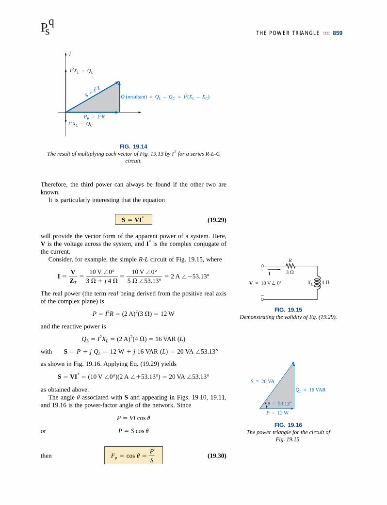
An additional verification can be derived by first considering theimpedance diagram of a series R-L-C circuit (Fig. 19.13). If we multi-ply each radius vector by the current squared (I2), we obtain the resultsshown in Fig. 19.14, which is the power triangle for a predominantlyinductive circuit.

Since the reactive power and average power are always angled 90° toeach other, the three powers are related by the Pythagorean theorem;that is,

(19.28)S2 � P2 � Q2

qtVC I

pC = –VC I sin 2qt QT

VL I

PL = VL I sin 2qt

QT = QL – QC = VL I – VC I = I(VL – VC) = I(IXL – IXC)

= I 2XL – I 2XC = I 2 (XL – XC)

FIG. 19.12

Demonstrating why the net reactive power is the difference between thatdelivered to inductive and capacitive elements.

+

XL

XC

XL – XC

Z

R

j

FIG. 19.13

Impedance diagram for a series R-L-C circuit.

4 �XL

+

–

I

V = 10 V 0°

R

3 �

FIG. 19.15

Demonstrating the validity of Eq. (19.29).

THE POWER TRIANGLE 859

Therefore, the third power can always be found if the other two areknown.

It is particularly interesting that the equation

(19.29)

will provide the vector form of the apparent power of a system. Here,V is the voltage across the system, and I* is the complex conjugate ofthe current.

Consider, for example, the simple R-L circuit of Fig. 19.15, where

I � � � � 2 A ��53.13°

The real power (the term real being derived from the positive real axisof the complex plane) is

P � I2R � (2 A)2(3 �) � 12 W

and the reactive power is

QL � I2XL � (2 A)2(4 �) � 16 VAR (L)

with S � P � j QL � 12 W � j 16 VAR (L) � 20 VA �53.13°

as shown in Fig. 19.16. Applying Eq. (19.29) yields

S � VI* � (10 V �0°)(2 A ��53.13°) � 20 VA �53.13°

as obtained above.The angle v associated with S and appearing in Figs. 19.10, 19.11,

and 19.16 is the power-factor angle of the network. Since

P � VI cos v

or P � S cos v

then (19.30)Fp � cos v � �P

S�

10 V �0°��5 � �53.13°

10 V �0°��3 � � j 4 �

V�ZT

S � VI*

Pqs

FIG. 19.14

The result of multiplying each vector of Fig. 19.13 by I2 for a series R-L-Ccircuit.

Q (resultant) = QL – QC = I2(XL – XC)

j

I2XC = QC

I2XL = QL

S = I2 Z

PR = I2R

S = 20 VA

P = 12 W

QL = 16 VAR

v = 53.13°

FIG. 19.16

The power triangle for the circuit of Fig. 19.15.

860 POWER (ac)

19.7 THE TOTAL P, Q, AND S

The total number of watts, volt-amperes reactive, and volt-amperes, andthe power factor of any system can be found using the following pro-cedure:

1. Find the real power and reactive power for each branch of thecircuit.

2. The total real power of the system (PT) is then the sum of theaverage power delivered to each branch.

3. The total reactive power (QT) is the difference between the reactivepower of the inductive loads and that of the capacitive loads.

4. The total apparent power is ST � �P�2T��� Q�2

T�.5. The total power factor is PT/ST.

There are two important points in the above tabulation. First, thetotal apparent power must be determined from the total average andreactive powers and cannot be determined from the apparent powers ofeach branch. Second, and more important, it is not necessary to con-sider the series-parallel arrangement of branches. In other words, thetotal real, reactive, or apparent power is independent of whether theloads are in series, parallel, or series-parallel. The following exampleswill demonstrate the relative ease with which all of the quantities ofinterest can be found.

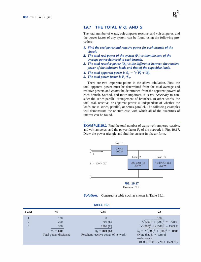
EXAMPLE 19.1 Find the total number of watts, volt-amperes reactive,and volt-amperes, and the power factor Fp of the network in Fig. 19.17.Draw the power triangle and find the current in phasor form.

Pqs

Solution: Construct a table such as shown in Table 19.1.

1500 VAR (C)300 W

700 VAR (L)200 W

0 VAR100 W

E = 100 V ∠ 0°

I

–

+

Load 2 Load 3

Load 1

FIG. 19.17

Example 19.1.

TABLE 19.1

Load W VAR VA

1 100 0 1002 200 700 (L) �(2�0�0�)2� �� (�7�0�0�)2� � 728.0

3 300 1500 (C) �(3�0�0�)2� �� (�1�5�0�0�)2� � 1529.71

PT � 600 QT � 800 (C) ST � �(6�0�0�)2� �� (�8�0�0�)2� � 1000Total power dissipated Resultant reactive power of network (Note that ST � sum of

each branch:1000 � 100 � 728 � 1529.71)

THE TOTAL P, Q, AND S 861

Thus,

Fp � � � 0.6 leading (C)

The power triangle is shown in Fig. 19.18.Since ST � VI � 1000 VA, I � 1000 VA/100 V � 10 A; and since v

of cos v � Fp is the angle between the input voltage and current:

I � 10 A ��53.13°

The plus sign is associated with the phase angle since the circuit is pre-dominantly capacitive.

EXAMPLE 19.2

a. Find the total number of watts, volt-amperes reactive, and volt-amperes, and the power factor Fp for the network of Fig. 19.19.

600 W�1000 VA

PT�ST

Pqs

ST = 1000 VA

PT = 600 W

QT = 800 VAR (C)

53.13° = cos –1 0.6

FIG. 19.18

Power triangle for Example 19.1.

b. Sketch the power triangle.c. Find the energy dissipated by the resistor over one full cycle of the

input voltage if the frequency of the input quantities is 60 Hz.d. Find the energy stored in, or returned by, the capacitor or inductor

over one half-cycle of the power curve for each if the frequency ofthe input quantities is 60 Hz.

Solutions:

a. I � � �100 V �0°

��10 � ��53.13°

100 V �0°���6 � � j 7 � � j 15 �

E�ZT

R

6 �

E = 100 V ∠ 0°

–

+

XL

I 7 �

XC 15 �

FIG. 19.19

Example 19.2.

� 10 A �53.13°VR � (10 A �53.13°)(6 � �0°) � 60 V �53.13°VL � (10 A �53.13°)(7 � �90°) � 70 V �143.13°VC � (10 A �53.13°)(15 � ��90°) � 150 V ��36.87°

PT � EI cos v � (100 V)(10 A) cos 53.13° � 600 W� I2R � (10 A)2(6 �) � 600 W

� � � 600 W

ST � EI � (100 V)(10 A) � 1000 VA� I2ZT � (10 A)2(10 �) � 1000 VA

� � � 1000 VA

QT � EI sin v � (100 V)(10 A) sin 53.13° � 800 VAR� QC � QL

� I2(XC � XL) � (10 A)2(15 � � 7 �) � 800 VAR

(100 V)2

�10 �

E2

�ZT

(60 V)2

�6

V2R

�R

862 POWER (ac)

QT � � � �

� 1500 VAR � 700 VAR � 800 VAR

Fp � � � 0.6 leading (C)

b. The power triangle is as shown in Fig. 19.20.

c. WR � � � 10 J

d. WL � � � � 1.86 J

WC � � � � 3.98 J

EXAMPLE 19.3 For the system of Fig. 19.21,

1500 J�

377

(150 V)(10 A)��

377 rad/s

VC I�q1

700 J�377

(70 V)(10 A)��(2p)(60 Hz)

VLI�q1

(60 V)(10 A)��

60 Hz

VRI�f1

600 W�1000 VA

PT�ST

(70 V)2

�7 �

(150 V)2

�15 �

V2L

�XL

V2C

�XC

Pqs

ST = 1000 VA

PT = 600 W

QT = 800 VAR (C)

53.13°

FIG. 19.20

Power triangle for Example 19.2.

R 9 �E = 208 V ∠ 0°

–

+

XC 12 �

6.4 kW 5 Hp

Heatingelements

1260-Wbulbs

Motor h = 82%

Fp = 0.72lagging

Capacitive load

a. Find the average power, apparent power, reactive power, and Fp foreach branch.

b. Find the total number of watts, volt-amperes reactive, and volt-amperes, and the power factor of the system. Sketch the power tri-angle.

c. Find the source current I.

Solutions:

a. Bulbs:Total dissipation of applied power

P1 � 12(60 W) � 720 W

Q1 � 0 VAR

S1 � P1 � 720 VA

Fp1� 1

Heating elements:Total dissipation of applied power

P2 � 6.4 kW

Q2 � 0 VAR

S2 � P2 � 6.4 kVA

Fp2� 1

FIG. 19.21

Example 19.3.

THE TOTAL P, Q, AND S 863

Motor:

h � Pi � � � 4548.78 W � P3

Fp � 0.72 lagging

P3 � S3 cos v S3 � � � 6317.75 VA

Also, v � cos�1 0.72 � 43.95°, so that

Q3 � S3 sin v � (6317.75 VA)(sin 43.95°)

� (6317.75 VA)(0.694) � 4384.71 VAR (L)

Capacitive load:

I � � � � 13.87 A �53.13°

P4 � I2R � (13.87 A)2• 9 � � 1731.39 W

Q4 � I2XC � (13.87 A)2• 12 � � 2308.52 VAR (C)

S4 � �P�24��� Q�2

4� � �(1�7�3�1�.3�9� W�)2� �� (�2�3�0�8�.5�2� V�A�R�)2�� 2885.65 VA

Fp � � � 0.6 leading

b. PT � P1 � P2 � P3 � P4

� 720 W � 6400 W � 4548.78 W � 1731.39 W

� 13,400.17 W

QT � Q1 Q2 Q3 Q4

� 0 � 0 � 4384.71 VAR (L) � 2308.52 VAR (C)

� 2076.19 VAR (L)

ST � �P�2T��� Q�2

T� � �(1�3�,4�0�0�.1�7� W�)2� �� (�2�0�7�6�.1�9� V�A�R�)2�� 13,560.06 VA

Fp � � � 0.988 lagging

v � cos�1 0.988 � 8.89°

Note Fig. 19.22.

13.4 kW��13,560.06 VA

PT�ST

1731.39 W��2885.65 VA

P4�S4

208 V �0°��15 � ��53.13°

208 V �0°��9 � � j 12 �

E�Z

4548.78 W��

0.72

P3�cos v

5(746 W)��

0.82

Po�h

Po�Pi

Pqs

ST = 13,560.06 VA

PT = 13.4 kW

QT = 2076.19 VAR (L)8.89°

FIG. 19.22

Power triangle for Example 19.3.

c. ST � EI I � � � 65.19 A

Lagging power factor: E leads I by 8.89°, and

I � 65.19 A ��8.89°

13,559.89 VA��

208 V

ST�E

ZT 1.6 �XL

R

1.2 �

864 POWER (ac)

EXAMPLE 19.4 An electrical device is rated 5 kVA, 100 V at a 0.6power-factor lag. What is the impedance of the device in rectangularcoordinates?

Solution:

S � EI � 5000 VA

Therefore, I � � 50 A

For Fp � 0.6, we have

v � cos�1 0.6 � 53.13°

Since the power factor is lagging, the circuit is predominantly induc-tive, and I lags E. Or, for E � 100 V �0°,

I � 50 A ��53.13°

However,

ZT � � � 2 � �53.13° � 1.2 � � j 1.6 �

which is the impedance of the circuit of Fig. 19.23.

19.8 POWER-FACTOR CORRECTION

The design of any power transmission system is very sensitive to themagnitude of the current in the lines as determined by the applied loads.Increased currents result in increased power losses (by a squared factorsince P � I2R) in the transmission lines due to the resistance of thelines. Heavier currents also require larger conductors, increasing theamount of copper needed for the system, and, quite obviously, theyrequire increased generating capacities by the utility company.

Every effort must therefore be made to keep current levels at a min-imum. Since the line voltage of a transmission system is fixed, theapparent power is directly related to the current level. In turn, thesmaller the net apparent power, the smaller the current drawn from thesupply. Minimum current is therefore drawn from a supply when S � Pand QT � 0. Note the effect of decreasing levels of QT on the length(and magnitude) of S in Fig. 19.24 for the same real power. Note alsothat the power-factor angle approaches zero degrees and Fp approaches1, revealing that the network is appearing more and more resistive at theinput terminals.

The process of introducing reactive elements to bring the power fac-tor closer to unity is called power-factor correction. Since most loadsare inductive, the process normally involves introducing elements withcapacitive terminal characteristics having the sole purpose of improvingthe power factor.

In Fig. 19.25(a), for instance, an inductive load is drawing a currentIL that has a real and an imaginary component. In Fig. 19.25(b), acapacitive load was added in parallel with the original load to raise thepower factor of the total system to the unity power-factor level. Notethat by placing all the elements in parallel, the load still receives thesame terminal voltage and draws the same current IL. In other words,the load is unaware of and unconcerned about whether it is hooked upas shown in Fig. 19.25(a) or Fig. 19.25(b).

100 V �0°��50 A ��53.13°

E�I

5000 VA�

100 V

Pqs

FIG. 19.23

Example 19.4.

v

QT

S

QT < QTS<S

v<θ

FIG. 19.24

Demonstrating the impact of power-factor correction on the power triangle of a network.

POWER-FACTOR CORRECTION 865

Solving for the source current in Fig. 19.25(b):

Is � IC � IL

� j IC(Imag) � IL(Re) � j IL(Imag)� IL(Re) � j [IL(Imag) � IC(Imag)]

If XC is chosen such that IC(Imag) � IL(Imag), then

Is � IL(Re) � j (0) � IL(Re) �0°

The result is a source current whose magnitude is simply equal to thereal part of the load current, which can be considerably less than themagnitude of the load current of Fig. 19.25(a). In addition, since thephase angle associated with both the applied voltage and the source cur-rent is the same, the system appears “resistive” at the input terminals,and all of the power supplied is absorbed, creating maximum efficiencyfor a generating utility.

EXAMPLE 19.5 A 5-hp motor with a 0.6 lagging power factor and anefficiency of 92% is connected to a 208-V, 60-Hz supply.a. Establish the power triangle for the load.b. Determine the power-factor capacitor that must be placed in parallel

with the load to raise the power factor to unity.c. Determine the change in supply current from the uncompensated to

the compensated system.d. Find the network equivalent of the above, and verify the conclusions.

Solutions:

a. Since 1 hp � 746 W,

Po � 5 hp � 5(746 W) � 3730 W

and Pi (drawn from the line) � � � 4054.35 W

Also, FP � cos v � 0.6

and v � cos�1 0.6 � 53.13°

Applying tan v �

we obtain QL � Pi tan v � (4054.35 W) tan 53.13°� 5405.8 VAR (L)

and

S � �P�2i �� Q�2

L� � �(4�0�5�4�.3�5� W�)2� �� (�5�4�0�5�.8� V�A�R�)2�� 6757.25 VA

QL�Pi

3730 W�

0.92

Po�h

Pqs

FIG. 19.25

Demonstrating the impact of a capacitive element on the power factor of anetwork.

Inductive load

E = E ∠ 0°

+

–

IL

(a)

XL > R

Fp < 1

L

R

Is

Fp = 1

ZT = ZT ∠ 0°

Xc

IL

E

+

–

(b)

IcInductive load

XL > R

Fp < 1

R

L

866 POWER (ac)

The power triangle appears in Fig. 19.26.

b. A net unity power-factor level is established by introducing acapacitive reactive power level of 5405.8 VAR to balance QL. Since

QC �

then XC � � � 8 �

and C � � � 331.6 mF

c. At 0.6Fp,

S � VI � 6757.25 VA

and I � � � 32.49 A

At unity Fp,

S � VI � 4054.35 VA

and I � � � 19.49 A

producing a 40% reduction in supply current.d. For the motor, the angle by which the applied voltage leads the cur-

rent is

v � cos�1 0.6 � 53.13°

and P � EIm cos v � 4054.35 W, from above, so that

Im � � � 32.49 A (as above)

resulting in

Im � 32.49 A ��53.13°

Therefore,

Zm � � � 6.4 � �53.13°

� 3.84 � � j 5.12 �

as shown in Fig. 19.27(a).

208 V �0°��32.49 A ��53.13°

E�Im

4054.35 W��(208 V)(0.6)

P�E cos v

4054.35 VA��

208 V

S�V

6757.25 VA��

208 V

S�V

1��(2p)(60 Hz)(8 �)

1�2pf XC

(208 V)2

��5405.8 VAR (C)

V2

�QC

V2

�XC

Pqs

S = 6757.25 VA

P = 4054.35 W

QL = 5404.45 VAR (L)

v = 53.13°

FIG. 19.26

Initial power triangle for the load of Example 19.5.

FIG. 19.27

Demonstrating the impact of power-factor corrections on the source current.

Is = Im = 32.49 A

E = 208 V ∠ 0°

+

–

(a)

R 10.64 � XL 8 �

Is = 19.49 A

E = 208 V ∠ 0°

+

–

(b)

XC 8 �

Im = 32.49 A

IC = 26 A

Motor Motor

Zm

XL 5.12 �

R 3.84 �

POWER-FACTOR CORRECTION 867

The equivalent parallel load is determined from

Y � �

� 0.156 S ��53.13° � 0.094 S � j 0.125 S

� �

as shown in Fig. 19.27(b).It is now clear that the effect of the 8-� inductive reactance can

be compensated for by a parallel capacitive reactance of 8 � using apower-factor correction capacitor of 332 mF.

Since

YT � � � �

Is � EYT � E� � � (208 V)� � � 19.54 A as above

In addition, the magnitude of the capacitive current can be deter-mined as follows:

IC � � � 26 A

EXAMPLE 19.6

a. A small industrial plant has a 10-kW heating load and a 20-kVAinductive load due to a bank of induction motors. The heating ele-ments are considered purely resistive (Fp � 1), and the inductionmotors have a lagging power factor of 0.7. If the supply is 1000 V at60 Hz, determine the capacitive element required to raise the powerfactor to 0.95.

b. Compare the levels of current drawn from the supply.

Solutions:

a. For the induction motors,

S � VI � 20 kVA

P � S cos v � (20 � 103 VA)(0.7) � 14 � 103 W

v � cos�1 0.7 � 45.6°

and

QL � VI sin v � (20 � 103 VA)(0.714) � 14.28 � 103 VAR (L)

The power triangle for the total system appears in Fig. 19.28.Note the addition of real powers and the resulting ST:

ST � �(2�4� k�W�)2� �� (�1�4�.2�8� k�V�A�R�)2� � 27.93 kVA

with IT � � � 27.93 A

The desired power factor of 0.95 results in an angle between Sand P of

v � cos�1 0.95 � 18.19°

27.93 kVA��

1000 VST�E

208 V�

8 �

E�XC

1�10.64 �

1�R

1�R

1��j XL

1�R

1��j XC

1�j 8 �

1�10.64 �

1��6.4 � �53.13°

1�Z

Pqs

QL = 14.28 kVAR (L)ST

30.75° 45.6°S

= 20 k

VA

P = 10 kW P = 14 kW

Heating Induction motors

FIG. 19.28

Initial power triangle for the load of Example 19.6.

868 POWER (ac)

changing the power triangle to that of Fig. 19.29:

with tan v � �Q

PT

′L� Q ′L � PT tan v � (24 � 103 W)(tan 18.19°)

� (24 � 103 W)(0.329) � 7.9 kVAR (L)

The inductive reactive power must therefore be reduced by

QL � Q′L � 14.28 kVAR (L) � 7.9 kVAR (L) � 6.38 kVAR (L)

Therefore, QC � 6.38 kVAR, and using

QC �

we obtain

XC � � � 156.74 �

and C � � � 16.93 mF

b. ST � �(2�4� k�W�)2� �� [�7�.9� k�V�A�R� (�L�)]�2�� 25.27 kVA

IT � � � 25.27 A

The new IT is

IT � 25.27 A �27.93 A (original)

19.9 WATTMETERS ANDPOWER-FACTOR METERS

The electrodynamometer wattmeter was introduced in Section 4.4 alongwith its movement and terminal connections. The same meter can beused to measure the power in a dc or an ac network using the same con-nection strategy; in fact, it can be used to measure the wattage of anynetwork with a periodic or a nonperiodic input.

The digital display wattmeter of Fig. 19.30 employs a sophisticatedelectronic package to sense the voltage and current levels and, throughthe use of an analog-to-digital conversion unit, display the proper digitson the display. It is capable of providing a digital readout for distortednonsinusoidal waveforms, and it can provide the phase power, totalpower, apparent power, reactive power, and power factor.

When using a wattmeter, the operator must take care not to exceedthe current, voltage, or wattage rating. The product of the voltage andcurrent ratings may or may not equal the wattage rating. In the high-power-factor wattmeter, the product of the voltage and current ratings isusually equal to the wattage rating, or at least 80% of it. For a low-power-factor wattmeter, the product of the current and voltage ratings ismuch greater than the wattage rating. For obvious reasons, the low-power-factor meter is used only in circuits with low power factors (totalimpedance highly reactive). Typical ratings for high-power-factor(HPF) and low-power-factor (LPF) meters are shown in Table 19.2.Meters of both high and low power factors have an accuracy of 0.5% to1% of full scale.

25.27 kVA��

1000 VST�E

1���(2p)(60 Hz)(156.74 �)

1�2pf XC

(103 V)2

��6.38 � 103 VAR

E2

�QC

E2

�XC

Pqs

FIG. 19.30

Digital wattmeter. (Courtesy of Yokogawa Corporation of America)

v = 18.19°PT = 24 kW

Q�L = 7.9 kVAR (L)

FIG. 19.29

Power triangle for the load of Example 19.6 after raising the power factor to 0.95.

EFFECTIVE RESISTANCE 869

As the name implies, power-factor meters are designed to read thepower factor of a load under operating conditions. Most are designed tobe used on single- or three-phase systems. Both the voltage and the cur-rent are typically measured using nonintrusive methods; that is, con-nections are made directly to the terminals for the voltage measure-ments, whereas clamp-on current transformers are used to sense thecurrent level, as shown for the power-factor meter of Fig. 19.31.

Once the power factor is known, most power-factor meters comewith a set of tables that will help define the power-factor capacitor thatshould be used to improve the power factor. Power-factor capacitors aretypically rated in kVAR, with typical ratings extending from 1 to 25 kVAR at 240 V and 1 to 50 kVAR at 480 V or 600 V.

19.10 EFFECTIVE RESISTANCE

The resistance of a conductor as determined by the equation R � r(l/A)is often called the dc, ohmic, or geometric resistance. It is a constantquantity determined only by the material used and its physical dimen-sions. In ac circuits, the actual resistance of a conductor (called theeffective resistance) differs from the dc resistance because of the vary-ing currents and voltages that introduce effects not present in dc circuits.

These effects include radiation losses, skin effect, eddy currents, andhysteresis losses. The first two effects apply to any network, while thelatter two are concerned with the additional losses introduced by thepresence of ferromagnetic materials in a changing magnetic field.

Experimental Procedure

The effective resistance of an ac circuit cannot be measured by the ratioV/I since this ratio is now the impedance of a circuit that may have bothresistance and reactance. The effective resistance can be found, how-ever, by using the power equation P � I2R, where

(19.31)

A wattmeter and an ammeter are therefore necessary for measuring theeffective resistance of an ac circuit.

Radiation Losses

Let us now examine the various losses in greater detail. The radiationloss is the loss of energy in the form of electromagnetic waves during thetransfer of energy from one element to another. This loss in energy

R eff � �I

P2�

Pqs

TABLE 19.2

Current Voltage WattageMeter Ratings Ratings Ratings

HPF 2.5 A 150 V 1500/750/3755.0 A 300 V

LPF 2.5 A 150 V 300/150/755.0 A 300 V

FIG. 19.31

Clamp-on power-factor meter. (Courtesy ofthe AEMC Corporation.)

Eddy currents

Coil

Ferromagnetic core

+

–

I

E

870 POWER (ac)

requires that the input power be larger to establish the same current I,causing R to increase as determined by Eq. (19.31). At a frequency of60 Hz, the effects of radiation losses can be completely ignored. How-ever, at radio frequencies, this is an important effect and may in factbecome the main effect in an electromagnetic device such as an antenna.

Skin Effect

The explanation of skin effect requires the use of some basic conceptspreviously described. Remember from Chapter 11 that a magnetic fieldexists around every current-carrying conductor (Fig. 19.32). Since theamount of charge flowing in ac circuits changes with time, the magneticfield surrounding the moving charge (current) also changes. Recall alsothat a wire placed in a changing magnetic field will have an inducedvoltage across its terminals as determined by Faraday’s law, e � N �(df/dt). The higher the frequency of the changing flux as determined byan alternating current, the greater the induced voltage will be.

For a conductor carrying alternating current, the changing magneticfield surrounding the wire links the wire itself, thus developing withinthe wire an induced voltage that opposes the original flow of charge orcurrent. These effects are more pronounced at the center of the conduc-tor than at the surface because the center is linked by the changing fluxinside the wire as well as that outside the wire. As the frequency of theapplied signal increases, the flux linking the wire will change at agreater rate. An increase in frequency will therefore increase thecounter-induced voltage at the center of the wire to the point where thecurrent will, for all practical purposes, flow on the surface of the con-ductor. At 60 Hz, the skin effect is almost noticeable. However, at radiofrequencies the skin effect is so pronounced that conductors are fre-quently made hollow because the center part is relatively ineffective.The skin effect, therefore, reduces the effective area through which thecurrent can flow, and it causes the resistance of the conductor, given bythe equation R↑ � r(l/A↓), to increase.

Hysteresis and Eddy Current Losses

As mentioned earlier, hysteresis and eddy current losses will appearwhen a ferromagnetic material is placed in the region of a changingmagnetic field. To describe eddy current losses in greater detail, we willconsider the effects of an alternating current passing through a coilwrapped around a ferromagnetic core. As the alternating current passesthrough the coil, it will develop a changing magnetic flux � linkingboth the coil and the core that will develop an induced voltage withinthe core as determined by Faraday’s law. This induced voltage and thegeometric resistance of the core RC � r(l/A) cause currents to be devel-oped within the core, icore � (eind /RC), called eddy currents. The cur-rents flow in circular paths, as shown in Fig. 19.33, changing directionwith the applied ac potential.

The eddy current losses are determined by

Peddy � i2eddyRcore

The magnitude of these losses is determined primarily by the type ofcore used. If the core is nonferromagnetic—and has a high resistivitylike wood or air—the eddy current losses can be neglected. In terms ofthe frequency of the applied signal and the magnetic field strength pro-

Pqs

I

Φ

FIG. 19.32

Demonstrating the skin effect on the effective resistance of a conductor.

FIG. 19.33

Defining the eddy current losses of a ferromagnetic core.

EFFECTIVE RESISTANCE 871

duced, the eddy current loss is proportional to the square of the fre-quency times the square of the magnetic field strength:

Peddy � f 2B2

Eddy current losses can be reduced if the core is constructed of thin,laminated sheets of ferromagnetic material insulated from one anotherand aligned parallel to the magnetic flux. Such construction reduces themagnitude of the eddy currents by placing more resistance in their path.

Hysteresis losses were described in Section 11.8. You will recallthat in terms of the frequency of the applied signal and the magneticfield strength produced, the hysteresis loss is proportional to the fre-quency to the 1st power times the magnetic field strength to the nthpower:

Phys � f 1Bn

where n can vary from 1.4 to 2.6, depending on the material under con-sideration.

Hysteresis losses can be effectively reduced by the injection of smallamounts of silicon into the magnetic core, constituting some 2% or 3%of the total composition of the core. This must be done carefully, how-ever, because too much silicon makes the core brittle and difficult tomachine into the shape desired.

EXAMPLE 19.7

a. An air-core coil is connected to a 120-V, 60-Hz source as shown inFig. 19.34. The current is found to be 5 A, and a wattmeter readingof 75 W is observed. Find the effective resistance and the inductanceof the coil.

Pqs

Wattmeter

I

E

+

–

120 V ∠ 0°

f = 60 Hz

CC

PCCoil

FIG. 19.34

The basic components required to determine the effective resistance andinductance of the coil.

b. A brass core is then inserted in the coil. The ammeter reads 4 A, andthe wattmeter 80 W. Calculate the effective resistance of the core. Towhat do you attribute the increase in value over that of part (a)?

c. If a solid iron core is inserted in the coil, the current is found to be2 A, and the wattmeter reads 52 W. Calculate the resistance and theinductance of the coil. Compare these values to those of part (a), andaccount for the changes.

872 POWER (ac)

Solutions:

a. R � � � 3 �

ZT � � � 24 �

XL � �Z�2T��� R�2� � �(2�4� ��)2� �� (�3� ��)2� � 23.81 �

and XL � 2pfL

or L � � � 63.16 mH

b. R � � � � 5 �

The brass core has less reluctance than the air core. Therefore, agreater magnetic flux density B will be created in it. Since Peddy �f 2B2, and Phys � f1Bn, as the flux density increases, the core lossesand the effective resistance increase.

c. R � � � � 13 �

ZT � � � 60 �

XL � �Z�2T��� R�2� � �(6�0� ��)2� �� (�1�3� ��)2� � 58.57 �

L � � � 155.36 mH

The iron core has less reluctance than the air or brass cores. There-fore, a greater magnetic flux density B will be developed in the core.Again, since Peddy � f 2B2, and Phys � f1Bn, the increased flux densitywill cause the core losses and the effective resistance to increase.

Since the inductance L is related to the change in flux by theequation L � N (df/di), the inductance will be greater for the ironcore because the changing flux linking the core will increase.

19.11 APPLICATIONS

Portable Power Generators

Even though it may appear that 120 V ac are just an extension cordaway, there are times—such as in a remote cabin, on a job site, or whilecamping—that we are reminded that not every corner of the globe isconnected to an electric power source. As you travel further away fromlarge urban communities, gasoline generators such as shown in Fig.19.35 appear in increasing numbers in hardware stores, lumber yards,and other retail establishments to meet the needs of the local commu-nity. Since ac generators are driven by a gasoline motor, they must beproperly ventilated and cannot be run indoors. Usually, because of thenoise and fumes that result, they are placed as far away as possible andare connected by a long, heavy-duty, weather-resistant extension cord.Any connection points must be properly protected and placed to ensurethat the connections will not sit in a puddle of water or be sensitive toheavy rain or snow. Although there is some effort involved in setting upgenerators and constantly ensuring that they have enough gas, mostusers will tell you that they are worth their weight in gold.

58.57 ��377 rad/s

XL�2pf

120 V�

2 A

E�I

52 ��

4

52 W�(2 A)2

P�I2

80 ��

16

80 W�(4 A)2

P�I2

23.81 ��377 rad/s

XL�2pf

120 V�

5 A

E�I

75 W�(5 A)2

P�I2

Pqs

FIG. 19.35

Single-phase portable generator. (Courtesy ofColeman Powermate, Inc.)

Continuous output power 1750–3000 W 2000–5000 W 2250–7500 W

Horsepower of gas motor 4–11 hp 5–14 hp 5–16 hp

Continuous At 120 V: 15–25 A At 120 V: 17–42 A At 120 V: 19–63 Aoutput current At 220 V(3f): 8–14 A At 220 V(3f): 9–23 A At 220 V(3f): 10–34 A

Output voltage 120 V or 120 V or 120 V or 3f: 120 V/220 V 3f: 120 V/220 V 3f: 120 V/220 V

Receptacles 2 2–4 2–4

Fuel tank 1⁄2 to 2 gallons 1⁄2 to 3 gallons 1 to 5 gallonsgasoline gasoline gasoline

APPLICATIONS 873

The vast majority of generators are built to provide between 1750 Wand 5000 W of power, although larger units can provide up to 20,000 W.At first encounter, you might assume that you can run the world on5000 W. However, keep in mind that the unit purchased should be ratedat least 20% above your expected load because of surge currents thatresult when appliances, motors, tools, etc., are turned on. Rememberthat even a light bulb develops a large turn-on current due to the cold,low-resistance state of the filament. If you work too closely to the ratedcapacity, experiences such as a severe drop in lighting can result whenan electric saw is turned on—almost to the point where it appears thatthe lights will go out altogether. Generators are like any other piece ofequipment: If you apply a load that is too heavy, they will shut down.Most have protective fuses or circuit breakers to ensure that the excur-sions above rated conditions are monitored and not exceeded beyondreason. The 20% protective barrier drops the output power from a5000-W unit to 4000 W, and already we begin to wonder about the loadwe can apply. Although 4000 W would be sufficient to run a number of60-W bulbs, a TV, an oil burner, and so on, troubles develop whenevera unit is hooked up for direct heating (such as heaters, hair dryers, andclothes dryers). Even microwaves at 1200 W command quite a powerdrain. Pile on a small electric heater at 1500 W with six 60-W bulbs(360 W), a 250-W TV, and a 250-W oil burner, and then turn on anelectric hair dryer at 1500 W—suddenly you are very close to yourmaximum of 4000 W. It doesn’t take long to push the limits when itcomes to energy-consuming appliances.

Table 19.3 provides a list of specifications for the broad range ofportable gasoline generators. Since the heaviest part of a generator isthe gasoline motor, anything over 5 hp gets pretty heavy, especiallywhen you add the weight of the gasoline. Most good units providingover 2400 W will have receptacles for 120 V and 220 V at various cur-rent levels, with an outlet for 12 V dc. They are also built so that theytolerate outdoor conditions of a reasonable nature and can run continu-ously for long periods of time. At 120 V, a 5000-W unit can provide amaximum current of about 42 A.

Pqs

TABLE 19.3

Specifications for portable gasoline-driven ac generators.

Business Sense

Because of the costs involved, every large industrial plant must contin-uously review its electric utility bill to ensure its accuracy and to con-sider ways that will keep it in check. As described in this chapter, the

874 POWER (ac)

power factor associated with the plant as a whole can have a measur-able effect on the drain current and therefore the kVA drain on thepower line. Power companies are aware of this problem and actuallyadd a surcharge if the power factor fades below about 0.9. In otherwords, to ensure that the load appears as resistive in nature as possible,the power company is asking every user to try to ensure that his powerfactor is between 0.9 and 1 so that the kW demand is very close to thekVA demand. Power companies do give some leeway, but they don’twant it to get out of hand.

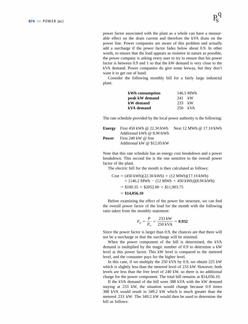
Consider the following monthly bill for a fairly large industrialplant:

kWh consumption 146.5 MWhpeak kW demand 241.5 kWkW demand 233.5 kWkVA demand 250.5 kVA

The rate schedule provided by the local power authority is the following:

Energy First 450 kWh @ 22.3¢/kWh Next 12 MWh @ 17.1¢/kWhAdditional kWh @ 8.9¢/kWh

Power First 240 kW @ freeAdditional kW @ $12.05/kW

Note that this rate schedule has an energy cost breakdown and a powerbreakdown. This second fee is the one sensitive to the overall powerfactor of the plant.

The electric bill for the month is then calculated as follows:

Cost � (450 kWh)(22.3¢/kWh) � (12 MWh)(17.1¢/kWh)� [146.2 MWh � (12 MWh � 450 kWh)](8.9¢/kWh)

� $100.35 � $2052.00 � $11,903.75

� $14,056.10

Before examining the effect of the power fee structure, we can findthe overall power factor of the load for the month with the followingratio taken from the monthly statement:

Fp � �P

P

a� � �

2

2

5

3

0

3

k

k

V

W

A� � 0.932

Since the power factor is larger than 0.9, the chances are that there willnot be a surcharge or that the surcharge will be minimal.

When the power component of the bill is determined, the kVAdemand is multiplied by the magic number of 0.9 to determine a kWlevel at this power factor. This kW level is compared to the meteredlevel, and the consumer pays for the higher level.

In this case, if we multiply the 250 kVA by 0.9, we obtain 225 kWwhich is slightly less than the metered level of 233 kW. However, bothlevels are less than the free level of 240 kW, so there is no additionalcharge for the power component. The total bill remains at $14,056.10.

If the kVA demand of the bill were 388 kVA with the kW demandstaying at 233 kW, the situation would change because 0.9 times388 kVA would result in 349.2 kW which is much greater than themetered 233 kW. The 349.2 kW would then be used to determine thebill as follows:

Pqs

COMPUTER ANALYSIS 875

349.2 kW � 240 kW � 109.2 kW

(109.2 kW)($12.05/kW) � $1315.86

which is significant.The total bill can then be determined as follows:

Cost � $14,056.10 � $1,315.86

� $15,371.96

Thus, the power factor of the load dropped to 233 kW/388 kVA � 0.6which would put an unnecessary additional load on the power plant. Itis certainly time to consider the power-factor-correction option asdescribed in this text. It is not uncommon to see large capacitors sittingat the point where power enters a large industrial plant to perform aneeded level of power-factor correction.

All in all, therefore, it is important to fully understand the impact ofa poor power factor on a power plant—whether you someday work forthe supplier or for the consumer.

19.12 COMPUTER ANALYSIS

PSpice

Power Curve: Resistor The computer analysis will begin with averification of the curves of Fig. 19.3 which show the in-phase relation-ship between the voltage and current of a resistor. The figure shows thatthe power curve is totally above the horizontal axis and that the curvehas a frequency twice the applied frequency and a peak value equal totwice the average value. First the simple schematic of Fig. 19.36 must

Pqs

FIG. 19.36

Using PSpice to review the power curve for a resistive element in an ac circuit.

876 POWER (ac) Pqs

be set up. Then, using the Time Domain(Transient) option to get aplot versus time and setting the Run to time to 1 ms and the Maximumstep size to 1 ms/1000 � 1 ms, we select OK and then the Run PSpiceicon to perform the simulation. Then Trace-Add Trace-V1(R) willresult in the curve appearing in Fig. 19.37. Next, Trace-Add Trace-I(R) will result in the curve for the current as appearing in Fig. 19.37.Finally the power curve will be plotted using Trace-Add Trace-V1(R)*I(R) from the basic power equation, and the larger curve of Fig.19.37 will result. The original plot had a y-axis that extended from �50to �50. Since all of the data points are from �20 to �50, the y-axiswas changed to this new range through Plot-Axis Settings-Y Axis-User Defined-(�20 to �50)-OK to obtain the plot of Fig. 19.37.

FIG. 19.37

The resulting plots for the power, voltage, and current for the resistor of Fig. 19.36.

You can distinguish between the curves by simply looking at thesymbol next to each quantity at the bottom left of the plot. In this case,however, to make it even clearer, a different color was selected for eachtrace by clicking on each trace with a right click, selecting Properties,and choosing the color and width of each curve. However, you can alsoadd text to the screen by selecting the ABC icon to obtain the TextLabel dialog box, entering the label such as P(R), and clicking OK.The label can then be placed anywhere on the screen. By selecting theToggle cursor key and then clicking on I(R) at the bottom of thescreen, we can use the cursor to find the maximum value of the current.At A1 � 250 ms or 1⁄4 of the total period of the input voltage, the cur-rent is a peak at 3.54 A. The peak value of the power curve can then befound by right-clicking on V1(R)*I(R), clicking on the graph, and thenfinding the peak value (also available by simply clicking on the Cursor

COMPUTER ANALYSIS 877

Peak icon to the right of the Toggle cursor key). It occurs at the samepoint as the maximum current at a level of 50 W. In particular, note thatthe power curve shows two cycles, while both vR and iR show only onecycle. Clearly, the power curve has twice the frequency of the appliedsignal. Also note that the power curve is totally above the zero line,indicating that power is being absorbed by the resistor through theentire displayed cycle. Further, the peak value of the power curve istwice the average value of the curve; that is, the peak value of 50 W istwice the average value of 25 W.

The results of the above simulation can be verified by performing thelonghand calculation using the rms value of the applied voltage. That is,

P � �VR

R2

� � �(1

40

�V)2

� � 25 W

Power Curves: Series R-L-C Circuit The network of Fig. 19.38,with its combination of elements, will now be used to demonstrate that,no matter what the physical makeup of the network, the average valueof the power curve established by the product of the applied voltage andresulting source current is equal to that dissipated by the network. At afrequency of 1 kHz, the reactance of the 1.273-mH inductor will be 8,and the reactance of the capacitor will be 4 �, resulting in a laggingnetwork. An analysis of the network will result in

ZT � 4 � � j4 � � 5.657 � �45°

with I � �ZE

T� � � 1.768 A ��45°

and P � I2R � (1.768 A)2 4 � � 12.5 W

10 V �0°��5.657 � �45°

Pqs

FIG. 19.38

Using PSpice to examine the power distribution in a series R-L-C circuit.

Pqs

The three curves of Fig. 19.39 were obtained using the SimulationOutput Variables V(E:�), I(R), and V(E:�)*I(R). The Run to timeunder the Simulation Profile listing was 20 ms, although 1 ms was cho-sen as the Maximum step size to ensure a good plot. In particular, notethat the horizontal axis does not start until t � 18 ms to ensure that weare in a steady-state mode and not in a transient stage (where the peakvalues of the waveforms could change with time). The horizontal axiswas set to extend from 18 ms to 20 ms by simply selecting Plot-AxisSettings-X Axis-User Defined-18ms to 20ms-OK. First note that thecurrent lags the applied voltage as expected for the lagging network.The phase angle between the two is 45° as determined above. Second,be aware that the elements were chosen so that the same scale could beused for the current and voltage. The vertical axis does not have a unitof measurement, so the proper units must be mentally added for eachplot. Using Plot-Label-Line, a line can be drawn across the screen atthe average power level of 12.5 W. A pencil will appear that can beclicked in place at the left edge at the 12.5-W level. The pencil can thenbe dragged across the page to draw the desired line. Once you are at theright edge, remove the pressure on the mouse, and the line is drawn.The different colors for the traces were obtained simply by right-clicking on a trace and responding to the choices under Properties.Note that the 12.5-W level is indeed the average value of the powercurve. It is interesting to note that the power curve dips below the axisfor only a short period of time. In other words, during the two visiblecycles, power is being absorbed by the circuit most of the time. The

878 POWER (ac)

FIG. 19.39

Plots of the applied voltage e, current iR � is, and power delivered ps � e isfor the circuit of Fig. 19.38.

PROBLEMS 879Pqs

small region below the axis is the return of energy to the network by thereactive elements. In general, therefore, the source must supply powerto the circuit most of the time, even though a good percentage of thepower may simply be delivering energy to the reactive elements andmay not being dissipated.

20 W

+

–E

Is

40 W

60 W

240 V

I1 I2

FIG. 19.40

Problem 1.

3 �+

–E = 50 V ∠ 0°

f = 60 Hz

5 � 9 �

RXC XL

FIG. 19.41

Problem 2.

PROBLEMS

SECTIONS 19.1 THROUGH 19.7

1. For the battery of bulbs (purely resistive) appearing inFig. 19.40:a. Determine the total power dissipation.b. Calculate the total reactive and apparent power.c. Find the source current Is.d. Calculate the resistance of each bulb for the specified

operating conditions.e. Determine the currents I1 and I2.

2. For the network of Fig. 19.41:a. Find the average power delivered to each element.b. Find the reactive power for each element.c. Find the apparent power for each element.d. Find the total number of watts, volt-amperes reactive,

and volt-amperes, and the power factor Fp of the cir-cuit.

e. Sketch the power triangle.f. Find the energy dissipated by the resistor over one full

cycle of the input voltage.g. Find the energy stored or returned by the capacitor

and the inductor over one half-cycle of the powercurve for each.

FIG. 19.42

Problem 3.

Load 1

+

–E = 100 V ∠9 0°

Load 2

600 VAR (C)100 W

200 VAR (L)0 W

Load 3

0 VAR300 W

Is

3. For the system of Fig. 19.42:a. Find the total number of watts, volt-amperes reactive,

and volt-amperes, and the power factor Fp.b. Draw the power triangle.c. Find the current Is.

FIG. 19.43

Problem 4.

Load 1

+

–E = 200 V ∠ 0° Load 2

600 VAR (C)500 W

1200 VAR (L)600 W Load 3

600 VAR (L)100 W

Is

4. For the system of Fig. 19.43:a. Find PT, QT, and ST.b. Determine the power factor Fp.c. Draw the power triangle.d. Find Is.

FIG. 19.44

Problem 5.

+

–E = 50 V ∠ 60°

Load 4

200 VAR (C)100 W

IsLoad 3

200 VAR (C)0 W

Load 1

100 VAR (L)200 W

Load 2

100 VAR (L)200 W

5. For the system of Fig. 19.44:a. Find PT, QT, and ST.b. Find the power factor Fp.c. Draw the power triangle.d. Find Is.

880 POWER (ac) Pqs

PROBLEMS 881Pqs

6. For the circuit of Fig. 19.45:a. Find the average, reactive, and apparent power for the

20-� resistor.b. Repeat part (a) for the 10-� inductive reactance.c. Find the total number of watts, volt-amperes reactive,

and volt-amperes, and the power factor Fp.d. Find the current Is.

FIG. 19.46

Problem 7.

R 2 �

+

–E = 20 V ∠ 0° XL

Is

4 �XC 5 �

f = 50 Hz

7. For the network of Fig. 19.46:a. Find the average power delivered to each element.b. Find the reactive power for each element.c. Find the apparent power for each element.d. Find PT, QT, ST, and Fp for the system.e. Sketch the power triangle.f. Find Is.

FIG. 19.47

Problem 8.

R 3 �+

–E = 50 V ∠6 0°

L

Is

4 �

C 10 �

f = 60 Hz

8. Repeat Problem 7 for the circuit of Fig. 19.47.

*9. For the network of Fig. 19.48:a. Find the average power delivered to each element.b. Find the reactive power for each element.c. Find the apparent power for each element.d. Find the total number of watts, volt-amperes reactive,

and volt-amperes, and the power factor Fp of the cir-cuit.

e. Sketch the power triangle.f. Find the energy dissipated by the resistor over one full

cycle of the input voltage.g. Find the energy stored or returned by the capacitor

and the inductor over one half-cycle of the powercurve for each.

FIG. 19.48

Problem 9.

R 30 �

+

–E = 50 V ∠ 0°

L

Is 0.1 H

C 100 mF

FIG. 19.45

Problem 6.

R 20 �

+

–E = 60 V ∠ 30° XL

Is

600 VAR (L)400 W

10 �

882 POWER (ac) Pqs

10. An electrical system is rated 10 kVA, 200 V at a 0.5 lead-ing power factor.a. Determine the impedance of the system in rectangular

coordinates.b. Find the average power delivered to the system.

11. An electrical system is rated 5 kVA, 120 V, at a 0.8 lag-ging power factor.a. Determine the impedance of the system in rectangular

coordinates.b. Find the average power delivered to the system.

*12. For the system of Fig. 19.49:a. Find the total number of watts, volt-amperes reactive,

and volt-amperes, and Fp.b. Find the current Is.c. Draw the power triangle.d. Find the type of elements and their impedance in

ohms within each electrical box. (Assume that all ele-ments of a load are in series.)

e. Verify that the result of part (b) is correct by findingthe current Is using only the input voltage E and theresults of part (d). Compare the value of Is with thatobtained for part (b).

FIG. 19.49

Problem 12.

Load 1

+

–E = 30 V ∠ 0°

Load 2

600 VAR (C)0 W

Is

200 VAR (L)300 W

*13. Repeat Problem 12 for the system of Fig. 19.50.

FIG. 19.50

Problem 13.

Load 2

+

–E = 100 V ∠ 0°

Load 3

0 VAR300 W

Is

500 VAR (L)600 W

Load 1

500 VAR (C)0 W

PROBLEMS 883Pqs

15. For the circuit of Fig. 19.52:a. Find the total number of watts, volt-amperes reactive,

and volt-amperes, and Fp.b. Find the voltage E.c. Find the type of elements and their impedance in each

box. (Assume that the elements within each box are inseries.)

Load 2

+

–E = 100 V ∠ 0°

Load 3

30 W40 VAR (L)

Is

100 VAR (L)Fp = 0

Load 1

200 WFp = 1

FIG. 19.51

Problem 14.

FIG. 19.52

Problem 15.

+

–I = 5 A ∠ 0°

Load 2

1000 W0.4Fp (leading)

Load 1

100 W0.8Fp (leading)E

SECTION 19.8 Power-Factor Correction

*16. The lighting and motor loads of a small factory establisha 10-kVA power demand at a 0.7 lagging power factor ona 208-V, 60-Hz supply.a. Establish the power triangle for the load.b. Determine the power-factor capacitor that must be

placed in parallel with the load to raise the power fac-tor to unity.

c. Determine the change in supply current from theuncompensated to the compensated system.

d. Repeat parts (b) and (c) if the power factor is in-creased to 0.9.

17. The load on a 120-V, 60-Hz supply is 5 kW (resistive),8 kVAR (inductive), and 2 kVAR (capacitive).a. Find the total kilovolt-amperes.b. Determine the Fp of the combined loads.

*14. For the circuit of Fig. 19.51:a. Find the total number of watts, volt-amperes reactive,

and volt-amperes, and Fp.b. Find the current Is.c. Find the type of elements and their impedance in each

box. (Assume that the elements within each box are inseries.)

884 POWER (ac) Pqs

c. Find the current drawn from the supply.d. Calculate the capacitance necessary to establish a

unity power factor.e. Find the current drawn from the supply at unity power

factor, and compare it to the uncompensated level.

18. The loading of a factory on a 1000-V, 60-Hz systemincludes:

20-kW heating (unity power factor)10-kW (Pi) induction motors (0.7 lagging power factor)5-kW lighting (0.85 lagging power factor)

a. Establish the power triangle for the total loading onthe supply.

b. Determine the power-factor capacitor required to raisethe power factor to unity.

c. Determine the change in supply current from theuncompensated to the compensated system.

SECTION 19.9 Wattmeters and Power-Factor Meters

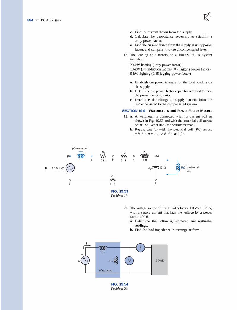
19. a. A wattmeter is connected with its current coil asshown in Fig. 19.53 and with the potential coil acrosspoints f-g. What does the wattmeter read?

b. Repeat part (a) with the potential coil (PC) acrossa-b, b-c, a-c, a-d, c-d, d-e, and f-e.

R2

3 �+

–E = 50 V ∠ 0° XC 12 �

f

gR1

2 �

CC(Current coil)

a b c

XL

3 �d

e

R3

1 �

PC (Potentialcoil)

FIG. 19.53

Problem 19.

20. The voltage source of Fig. 19.54 delivers 660 VA at 120 V,with a supply current that lags the voltage by a powerfactor of 0.6.a. Determine the voltmeter, ammeter, and wattmeter

readings.b. Find the load impedance in rectangular form.

FIG. 19.54

Problem 20.

I

I

E

+

–Wattmeter

CC

PC V LOAD

GLOSSARY 885Pqs

SECTION 19.10 Effective Resistance

21. a. An air-core coil is connected to a 200-V, 60-Hz source.The current is found to be 4 A, and a wattmeterreading of 80 W is observed. Find the effectiveresistance and the inductance of the coil.

b. A brass core is inserted in the coil. The ammeter reads3 A, and the wattmeter reads 90 W. Calculate the effec-tive resistance of the core. Explain the increase overthe value of part (a).

c. If a solid iron core is inserted in the coil, the currentis found to be 2 A, and the wattmeter reads 60 W. Cal-culate the resistance and inductance of the coil. Com-pare these values to the values of part (a), and accountfor the changes.

22. a. The inductance of an air-core coil is 0.08 H, and theeffective resistance is 4 � when a 60-V, 50-Hz sourceis connected across the coil. Find the current passingthrough the coil and the reading of a wattmeter acrossthe coil.

b. If a brass core is inserted in the coil, the effectiveresistance increases to 7 �, and the wattmeter reads 30 W. Find the current passing through the coil andthe inductance of the coil.

c. If a solid iron core is inserted in the coil, the effectiveresistance of the coil increases to 10 �, and the cur-rent decreases to 1.7 A. Find the wattmeter reading andthe inductance of the coil.

SECTION 19.12 Computer Analysis

PSpice or Electronics Workbench

23. Using PSpice or EWB, obtain a plot of reactive powerfor a pure capacitor of 636.62 mF at a frequency of 1 kHzfor one cycle of the input voltage using an applied volt-age E � 10 V �0°. On the same graph, plot both theapplied voltage and the resulting current. Apply appropri-ate labels to the resulting curves to generate results simi-lar to those in Fig. 19.37.

24. Repeat the analysis of Fig. 19.38 for a parallel R-L-C net-work of the same values and frequency.

25. Plot both the applied voltage and the source current onthe same set of axes for the network of Fig. 19.27(b), andshow that they are both in phase due to the resulting unitypower factor.

Programming Language (C��, QBASIC, Pascal, etc.)

26. Write a program that provides a general solution for thenetwork of Fig. 19.19. That is, given the resistance orreactance of each element and the source voltage at zerodegrees, calculate the real, reactive, and apparent powerof the system.

27. Write a program that will demonstrate the effect ofincreasing reactive power on the power factor of a sys-tem. Tabulate the real power, reactive power, and powerfactor of the system for a fixed real power and a reactivepower that starts at 10% of the real power and continuesthrough to five times the real power in increments of 10%of the real power.

GLOSSARY

Apparent power The power delivered to a load without con-sideration of the effects of a power-factor angle of the load.It is determined solely by the product of the terminal volt-age and current of the load.

Average (real) power The delivered power dissipated in theform of heat by a network or system.

Eddy currents Small, circular currents in a paramagneticcore causing an increase in the power losses and the effec-tive resistance of the material.

Effective resistance The resistance value that includes theeffects of radiation losses, skin effect, eddy currents, andhysteresis losses.

Hysteresis losses Losses in a magnetic material introducedby changes in the direction of the magnetic flux within thematerial.

Power-factor correction The addition of reactive compo-nents (typically capacitive) to establish a system power fac-tor closer to unity.

Radiation losses The loss of energy in the form of electro-magnetic waves during the transfer of energy from one ele-ment to another.

Reactive power The power associated with reactive ele-ments that provides a measure of the energy associated withsetting up the magnetic and electric fields of inductive andcapacitive elements, respectively.

Skin effect At high frequencies, a counter-induced voltagebuilds up at the center of a conductor, resulting in an increasedflow near the surface (skin) of the conductor and a sharpreduction near the center.As a result, the effective area of con-duction decreases and the resistance increases as defined bythe basic equation for the geometric resistance of a conductor.