Embed Size (px)
DESCRIPTION
NUS geotechnical engineering - CE5101
Citation preview
CE5101 Consolidation and SeepageLecture 6
Prof Harry TanOCT 2011
1
CE 5101 Lecture 6 – 1D ConsolidationConsolidation
Oct 2011
Prof Harry Tan
1
Outline
• Terzaghi Theory
U f l El ti S l ti• Useful Elastic Solutions
• Oedometer Tests
• FEM Theory
• FEM compared with Terzaghi
• Consolidation of Realistic Soils
2
• Example of Consolidation in Reclaimed Land
• Secondary Compression and Creep
CE5101 Consolidation and SeepageLecture 6
Prof Harry TanOCT 2011
2
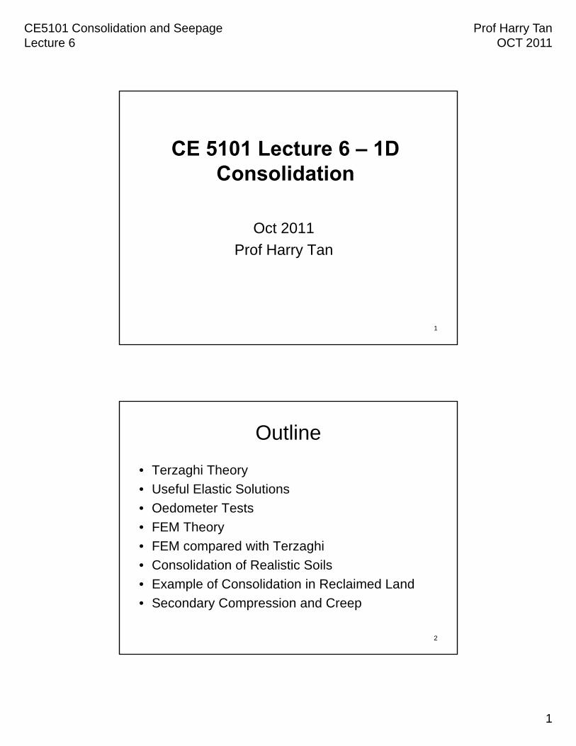
Terzaghi 1D Vertical Flow
• Formulation of Theory
• Useful Approximations
• Elastic Solutions
3
1D CONSOLIDATION
Assumptions made:
soil is fully saturated
pore water is incompressible
Darcy's law is valid
isotropic (constant) permeability
linear elastic soil behaviour
4
load applied instantaneously
one-dimensional problem (length of applied load > ∞)
CE5101 Consolidation and SeepageLecture 6
Prof Harry TanOCT 2011
3
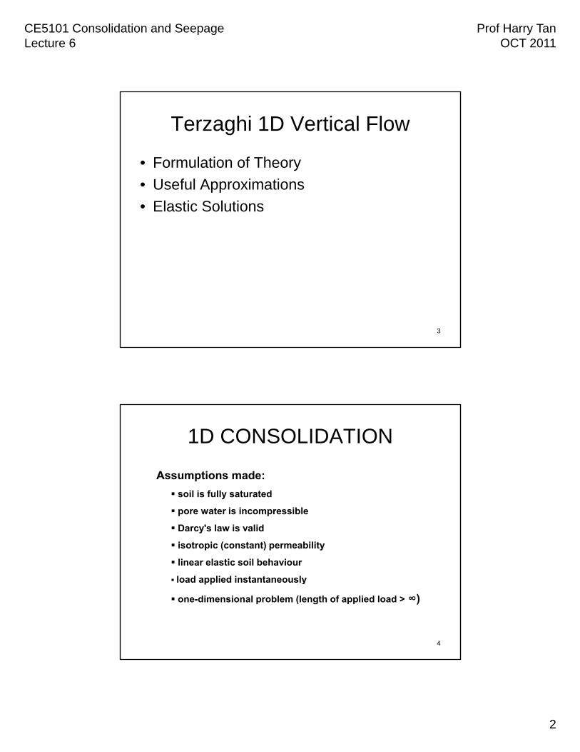
1D CONSOLIDATION
soft clay layerfully saturated
p = p
initialground surface
apply surcharge load rapidly
p = p + p t = 0
z
pw = pw, o
´ = ´
rigid impermeable layer
D
rigid impermeable layer
pw = pw, o + pw, t=o
pw, t=o =
´ = ´
t = 0
settlement st
consolidation takes place
settlement s
consolidation process completed
5rigid impermeable layer
pw = pw, o + pw, t
pw, t = t´
´ = ´ + t´
0 < t < ∞
rigid impermeable layer
pw = pw, o
´ = ´ +
t = ∞
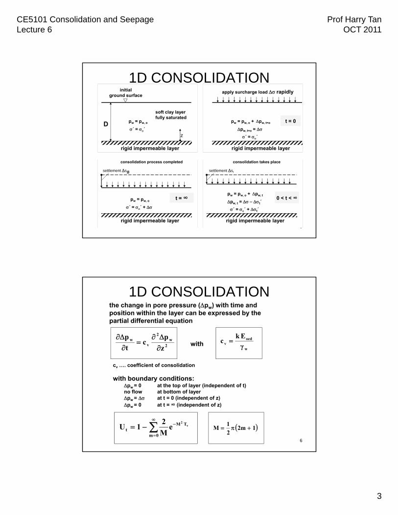
1D CONSOLIDATION
2 Ek
the change in pore pressure (pw) with time and position within the layer can be expressed by the partial differential equation
2w
2
vw
z
pc
t
p
w
oedv γ
Ekc with
cv …. coefficient of consolidation
with boundary conditions:pw = 0 at the top of layer (independent of t)no flow at bottom of layer
6
0m
TMt
v2
eM
21U
ypw = at t = 0 (independent of z)pw = 0 at t = ∞ (independent of z)
1m22
1M
CE5101 Consolidation and SeepageLecture 6
Prof Harry TanOCT 2011
4
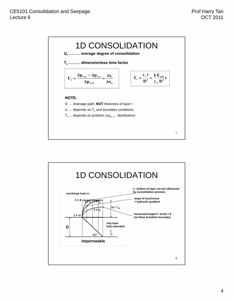
1D CONSOLIDATIONUt ……… average degree of consolidation
Tv ……… dimensionless time factor
tDγ
Ek
D
tcT
2w
oed2
vv
s
s
p
ppU t
0,w
t,wo,wt
NOTE:
D .... drainage path, NOT thickness of layer !
7
g p , y
U .... depends on Tv and boundary conditions
Tv ... depends on problem (pw, o - distribution)
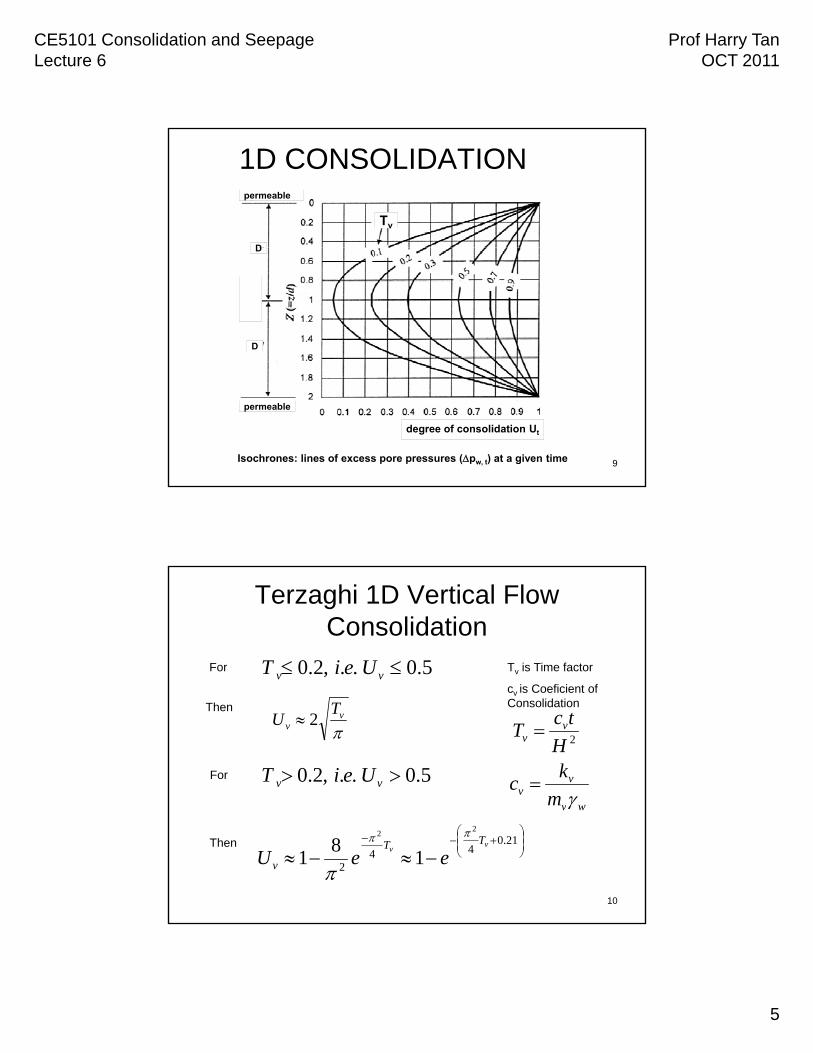
1D CONSOLIDATIONt1: bottom of layer not yet influenced by consolidation processsurcharge load
clay layerfully saturated
/ w
t = 0 t = t1 t = t2
t = t = t3
horizontal tangent > dv/dz = 0 (no flow) at bottom boundary
slope of Isochrones > hydraulic gradient
D
8
z
impermeable
45°
CE5101 Consolidation and SeepageLecture 6
Prof Harry TanOCT 2011
5
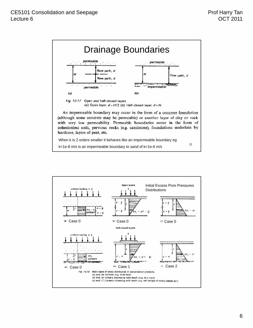
1D CONSOLIDATIONpermeable
D
Tv
D
D
9
degree of consolidation Ut
permeable
Isochrones: lines of excess pore pressures (pw, t) at a given time
Terzaghi 1D Vertical Flow Consolidation
5.0..,2.0 vv UeiTFor Tv is Time factor
i C fi i t f
v
v
TU 2
Then
For 5.0..,2.0 vv UeiT
cv is Coeficient of Consolidation
vv
vv
m
kc
H
tcT
2
10
21.0
442
22
18
1v
vTT
v eeU
Then
wvm
CE5101 Consolidation and SeepageLecture 6
Prof Harry TanOCT 2011
6
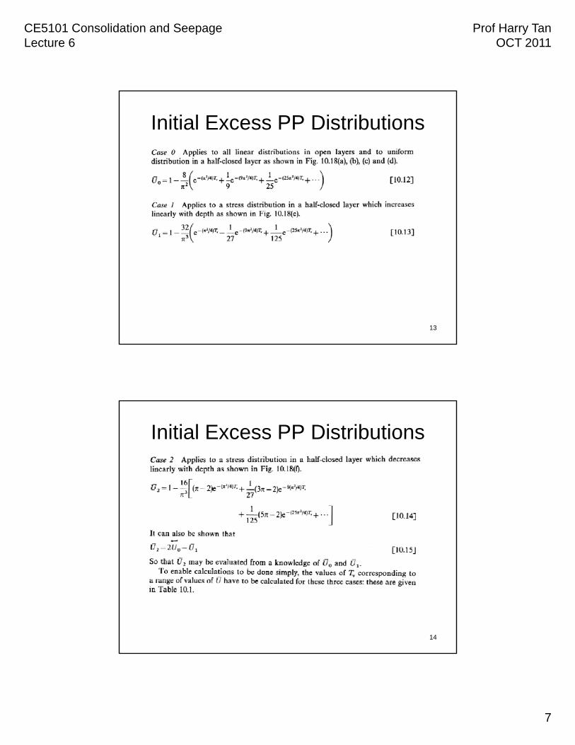
Drainage Boundaries
11
When k is 2 orders smaller it behaves like an impermeable boundary eg
k=1e-8 m/s is an impermeable boundary to sand of k=1e-6 m/s
Initial Excess Pore Pressures Distributions
Case 0 Case 0Case 0
12
Case 0 Case 1 Case 2
CE5101 Consolidation and SeepageLecture 6
Prof Harry TanOCT 2011
7
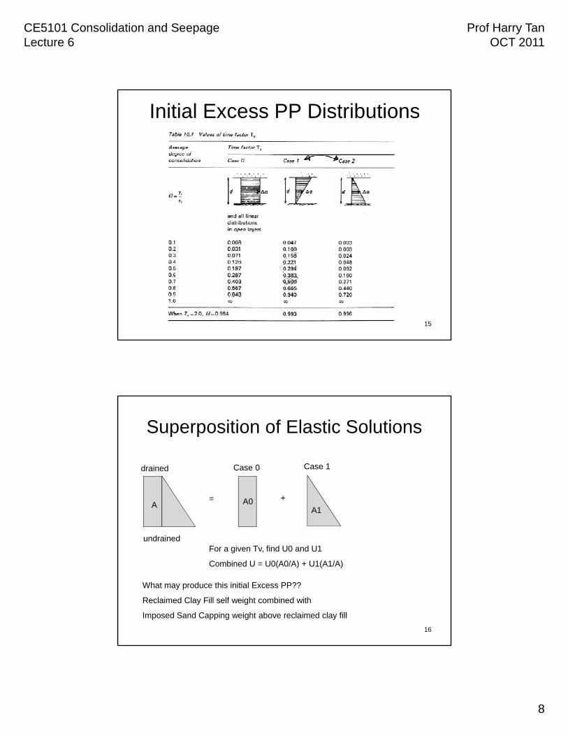
Initial Excess PP Distributions
13
Initial Excess PP Distributions
14
CE5101 Consolidation and SeepageLecture 6
Prof Harry TanOCT 2011
8
Initial Excess PP Distributions
15
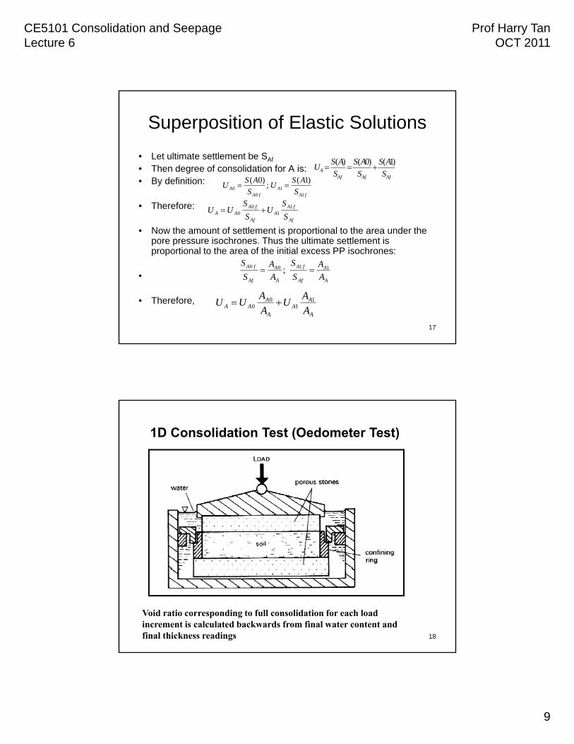
Superposition of Elastic Solutions
drained Case 0 Case 1
undrained
= +A A0
A1
For a given Tv, find U0 and U1
Combined U = U0(A0/A) + U1(A1/A)
16
Combined U = U0(A0/A) + U1(A1/A)
What may produce this initial Excess PP??
Reclaimed Clay Fill self weight combined with
Imposed Sand Capping weight above reclaimed clay fill
CE5101 Consolidation and SeepageLecture 6
Prof Harry TanOCT 2011
9
Superposition of Elastic Solutions
• Let ultimate settlement be SAf
• Then degree of consolidation for A is: A S
AS
S
AS
S
ASU
)1()0()(
• By definition:
• Therefore:
• Now the amount of settlement is proportional to the area under the pore pressure isochrones. Thus the ultimate settlement is proportional to the area of the initial excess PP isochrones:
AfAfAf SSS
fAA
fAA S
ASU
S
ASU
11
00
)1(;
)0(
Af
fAA
Af
fAAA S
SU
S
SUU 1
10
0
17
•
• Therefore,
A
A
Af
fA
A
A
Af
fA
A
A
S
S
A
A
S
S1100 ;
A
AA
A
AAA A
AU
A
AUU 1
10
0
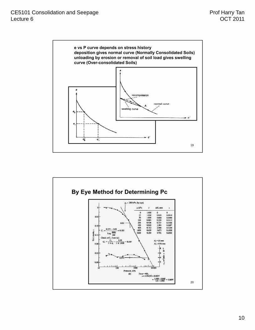
1D Consolidation Test (Oedometer Test)
18
Void ratio corresponding to full consolidation for each load increment is calculated backwards from final water content and final thickness readings
CE5101 Consolidation and SeepageLecture 6
Prof Harry TanOCT 2011
10
e vs P curve depends on stress historydeposition gives normal curve (Normally Consolidated Soils)unloading by erosion or removal of soil load gives swelling curve (Over-consolidated Soils)
19
By Eye Method for Determining Pc
20
CE5101 Consolidation and SeepageLecture 6
Prof Harry TanOCT 2011
11
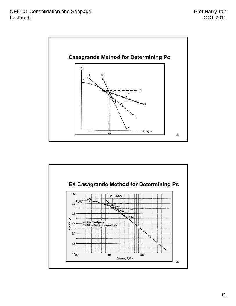
Casagrande Method for Determining Pc
21
EX Casagrande Method for Determining Pc
22
CE5101 Consolidation and SeepageLecture 6
Prof Harry TanOCT 2011
12
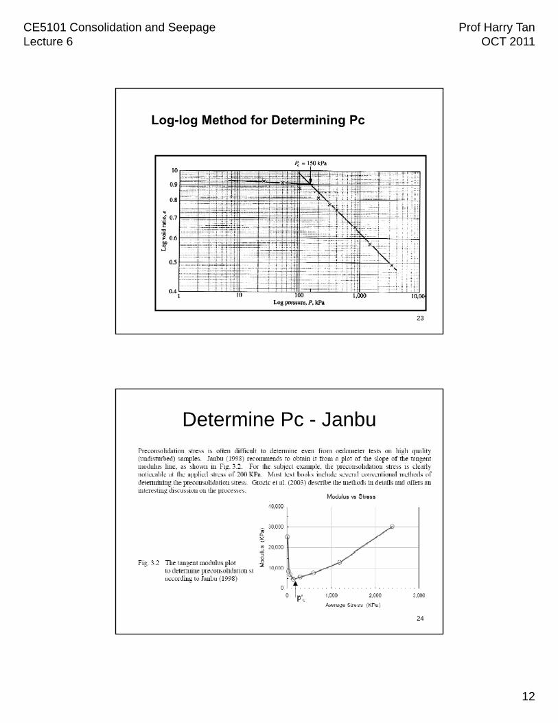
Log-log Method for Determining Pc
23
Determine Pc - Janbu
PcPc
24
CE5101 Consolidation and SeepageLecture 6
Prof Harry TanOCT 2011
13
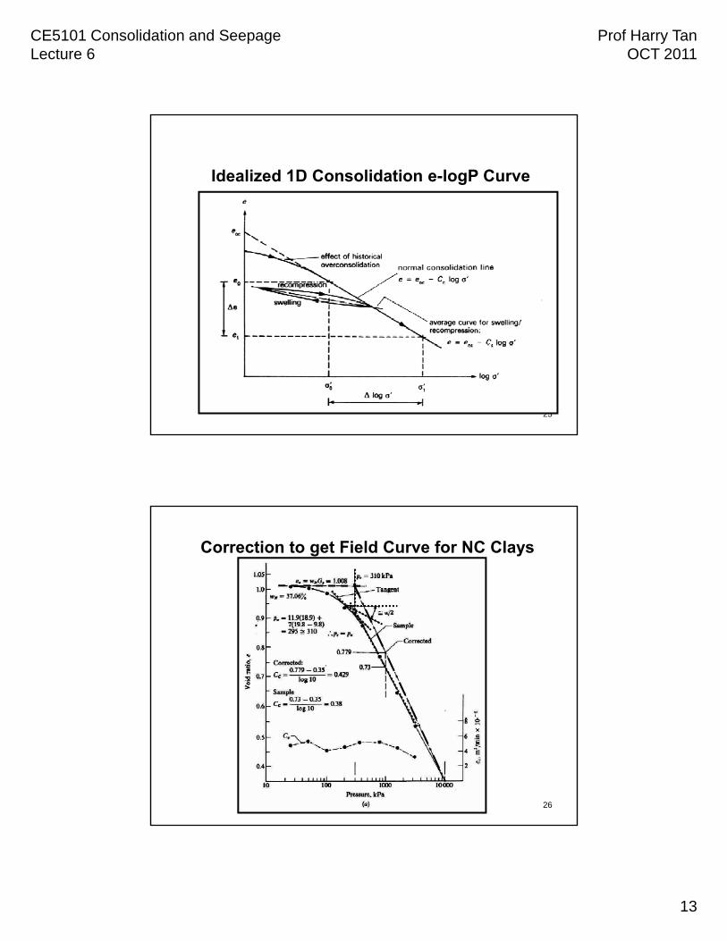
Idealized 1D Consolidation e-logP Curve
25
Correction to get Field Curve for NC Clays
26
CE5101 Consolidation and SeepageLecture 6
Prof Harry TanOCT 2011
14
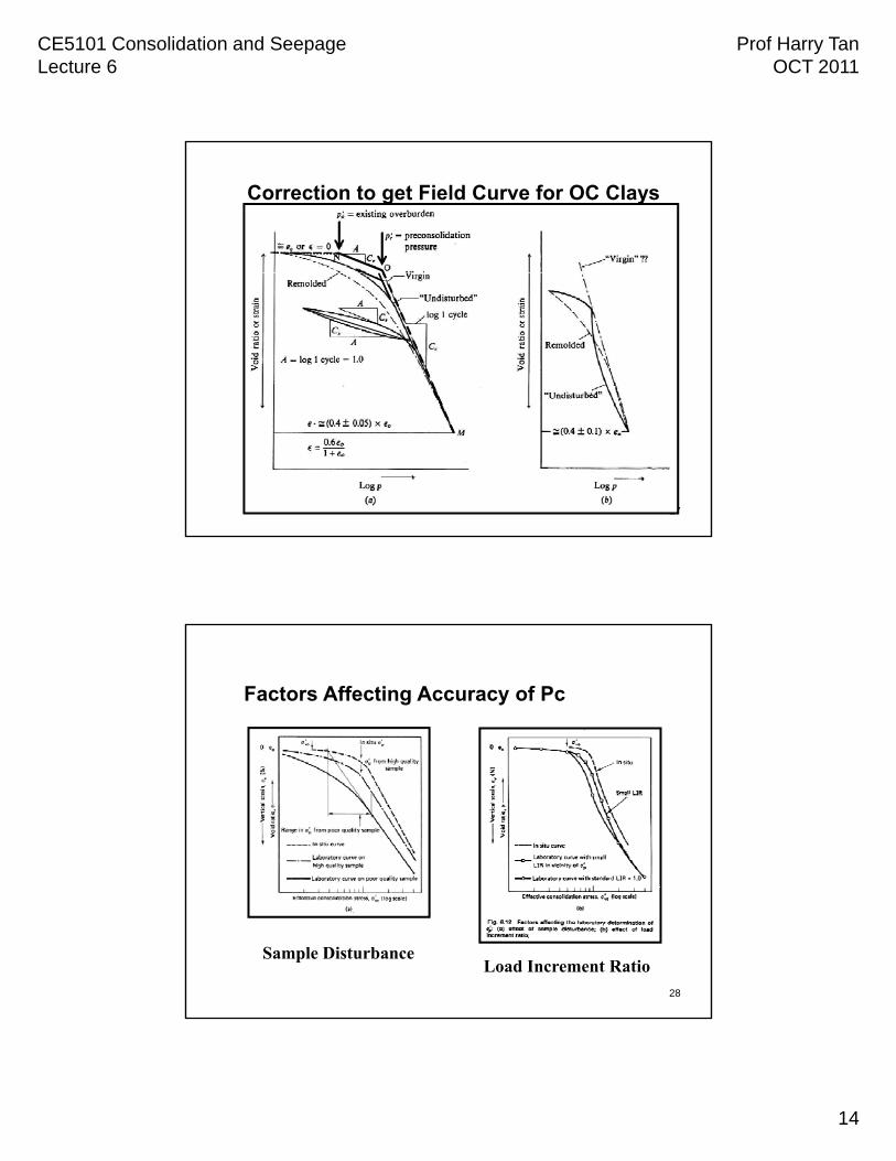
Correction to get Field Curve for OC Clays
27
Factors Affecting Accuracy of Pc
28
Sample DisturbanceLoad Increment Ratio
CE5101 Consolidation and SeepageLecture 6
Prof Harry TanOCT 2011
15
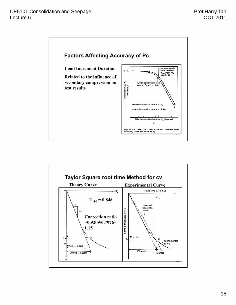
Factors Affecting Accuracy of Pc
Load Increment Duration
Related to the influence of secondary compression on test results
29
Taylor Square root time Method for cvExperimental CurveTheory Curve
T 0 848
Correction ratio =0.9209/0.7976=1.15
Tv90 = 0.848
30
CE5101 Consolidation and SeepageLecture 6
Prof Harry TanOCT 2011
16
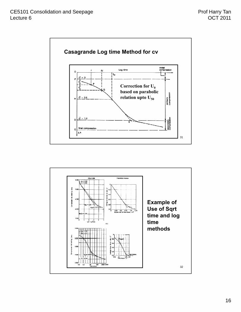
Casagrande Log time Method for cv
Correction for U0
based on parabolic relation upto U50
31
Example ofExample of Use of Sqrt time and log time methods
32
CE5101 Consolidation and SeepageLecture 6
Prof Harry TanOCT 2011
17
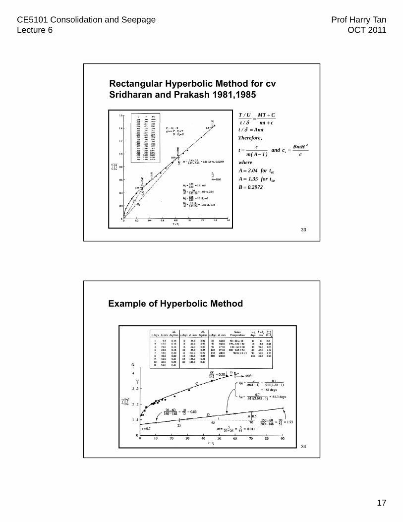
Rectangular Hyperbolic Method for cvSridharan and Prakash 1981,1985
cmt
CMT
/t
U/T
tfor35.1A
tfor04.2A
where
c
BmHcand
)1A(m
ct
,Therefore
Amt/tcmt/t
90
60
2
v
33
2972.0B
Example of Hyperbolic Method
34
CE5101 Consolidation and SeepageLecture 6
Prof Harry TanOCT 2011
18
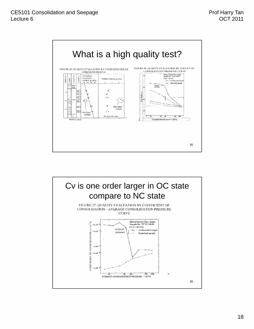
What is a high quality test?
35
Cv is one order larger in OC state compare to NC state
36
CE5101 Consolidation and SeepageLecture 6
Prof Harry TanOCT 2011
19
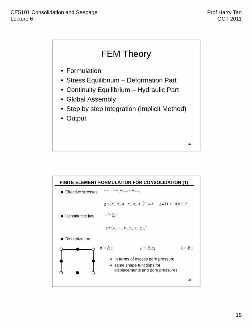
FEM Theory
• Formulation
• Stress Equilibrium – Deformation Part
• Continuity Equilibrium – Hydraulic Part
• Global Assembly
• Step by step Integration (Implicit Method)
37
• Output
FINITE ELEMENT FORMULATION FOR CONSOLIDATION (1)
Effective stresses
Constitutive law
Discretization
38
In terms of excess pore pressure
same shape functions for displacements and pore pressures
CE5101 Consolidation and SeepageLecture 6
Prof Harry TanOCT 2011
20
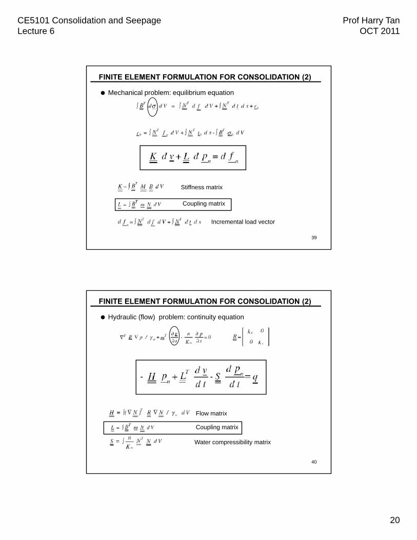
FINITE ELEMENT FORMULATION FOR CONSOLIDATION (2)
Mechanical problem: equilibrium equation
Stiffness matrix
39
Stiffness matrix
Coupling matrix
Incremental load vector
FINITE ELEMENT FORMULATION FOR CONSOLIDATION (2)
Hydraulic (flow) problem: continuity equation
Flow matrix
40
Flow matrix
Coupling matrix
Water compressibility matrix
CE5101 Consolidation and SeepageLecture 6
Prof Harry TanOCT 2011
21
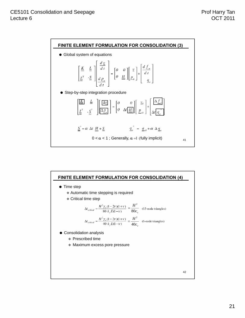
FINITE ELEMENT FORMULATION FOR CONSOLIDATION (3)
Global system of equations
Step-by-step integration procedure
410 < < 1 ; Generally, fully implicit)
FINITE ELEMENT FORMULATION FOR CONSOLIDATION (4)
Time step
Automatic time stepping is required
Critical time step
H 2
Consolidation analysis
Prescribed time
vc80
vc
H
40
2
42
Maximum excess pore pressure
CE5101 Consolidation and SeepageLecture 6
Prof Harry TanOCT 2011
22
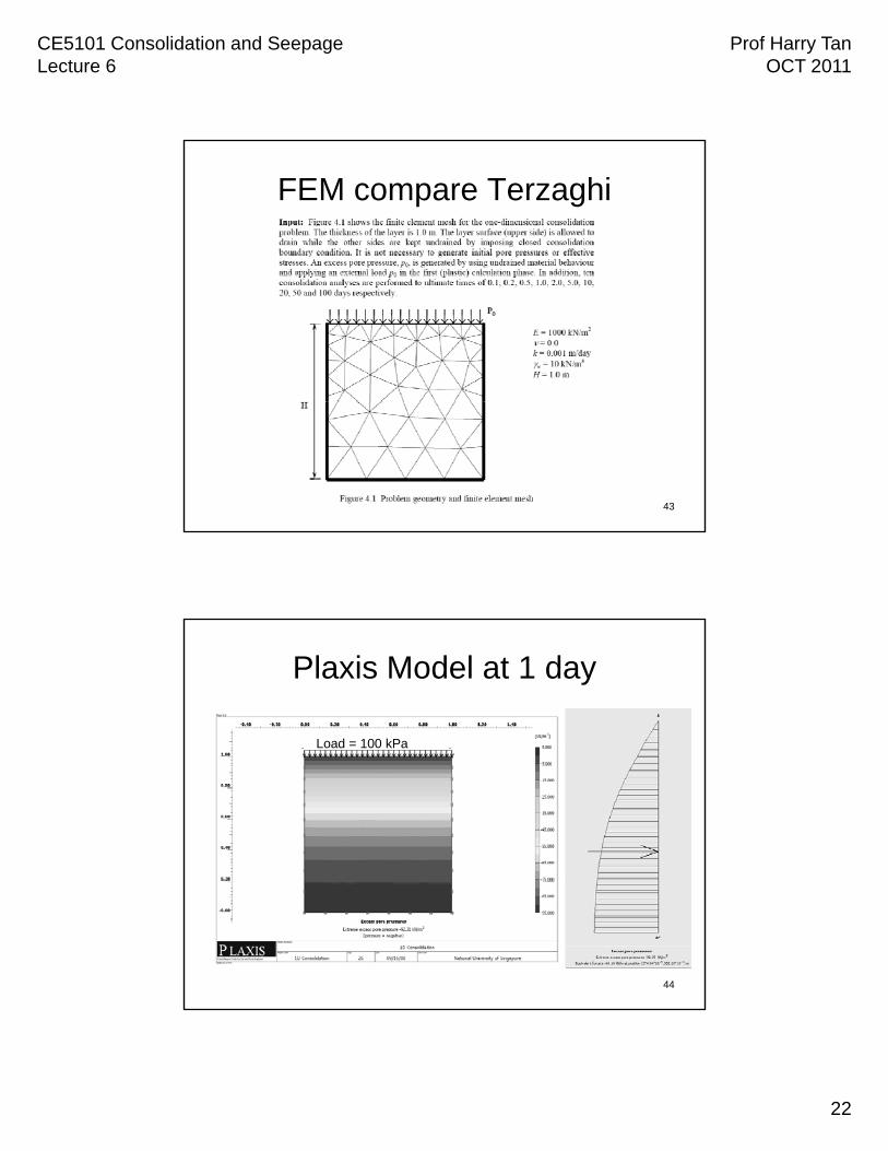
FEM compare Terzaghi
43
Plaxis Model at 1 day
Load = 100 kPa
44
CE5101 Consolidation and SeepageLecture 6
Prof Harry TanOCT 2011
23
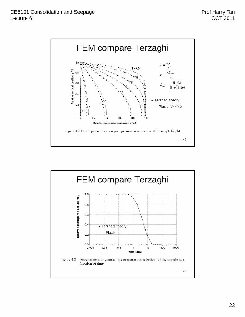
FEM compare Terzaghi
Terzhagi theory
Plaxis Ver 9.0
45
FEM compare Terzaghi
Terzhagi theory
Plaxis
46
CE5101 Consolidation and SeepageLecture 6
Prof Harry TanOCT 2011
24
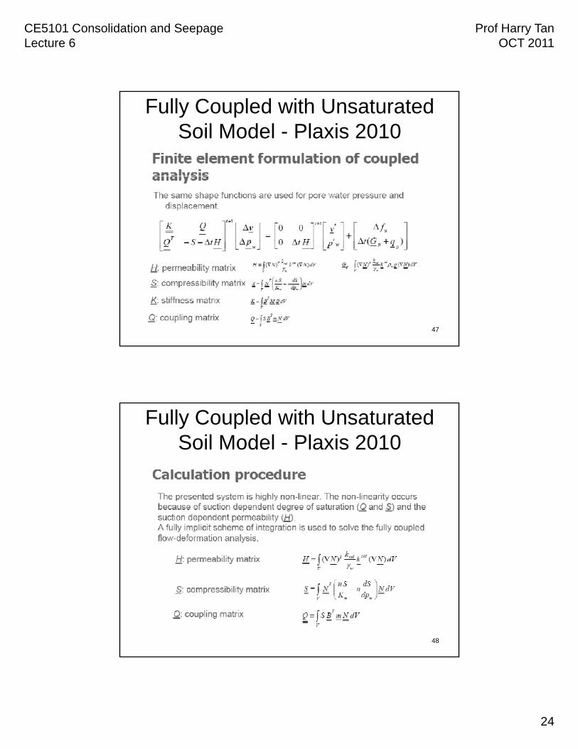
Fully Coupled with Unsaturated Soil Model - Plaxis 2010
47
Fully Coupled with Unsaturated Soil Model - Plaxis 2010
48
CE5101 Consolidation and SeepageLecture 6
Prof Harry TanOCT 2011
25
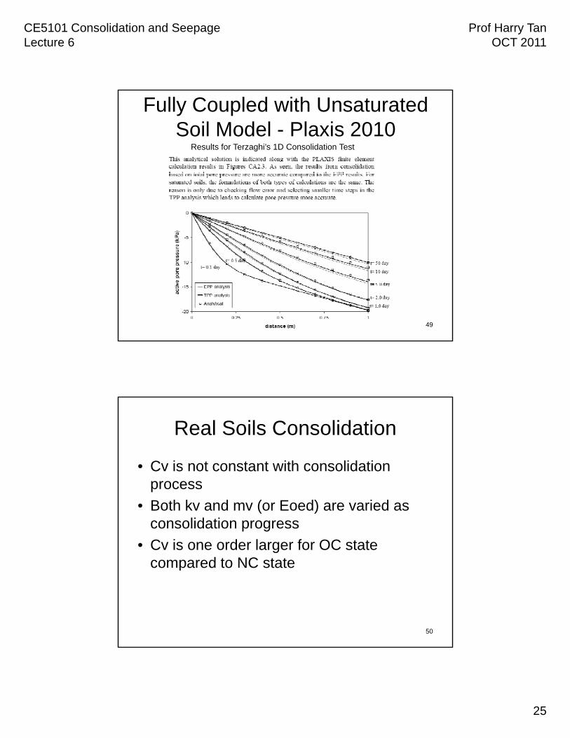
Fully Coupled with Unsaturated Soil Model - Plaxis 2010
Results for Terzaghi’s 1D Consolidation Test
49
Real Soils Consolidation
• Cv is not constant with consolidation process
• Both kv and mv (or Eoed) are varied as consolidation progress
• Cv is one order larger for OC state compared to NC state
50
compared to NC state
CE5101 Consolidation and SeepageLecture 6
Prof Harry TanOCT 2011
26
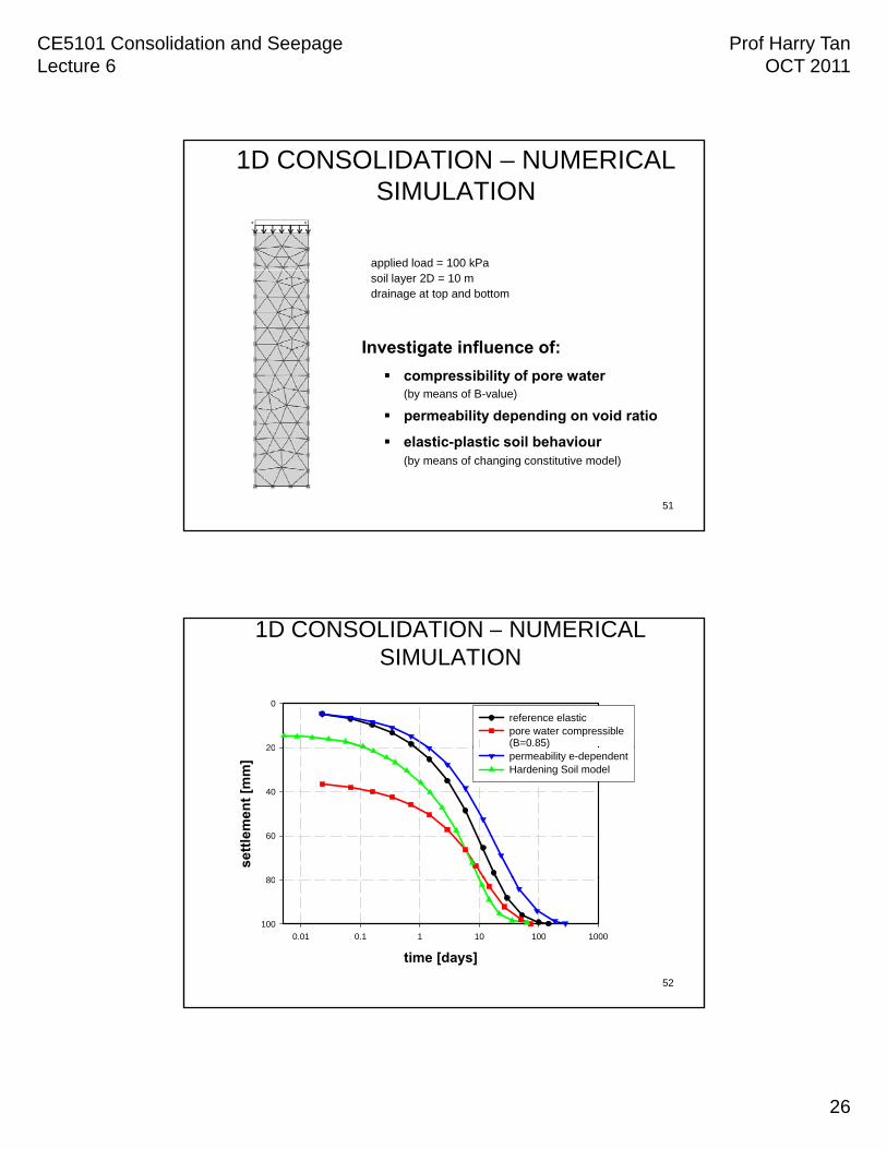
1D CONSOLIDATION – NUMERICAL SIMULATION
applied load = 100 kPa
Investigate influence of:
compressibility of pore water (by means of B-value)
soil layer 2D = 10 mdrainage at top and bottom
51
permeability depending on void ratio
elastic-plastic soil behaviour(by means of changing constitutive model)
1D CONSOLIDATION – NUMERICAL SIMULATION
0
20
reference elasticpore water compressible (B=0.85)
sett
lem
ent
[mm
]
20
40
60
80
( )permeability e-dependentHardening Soil model
52
time [days]
0.01 0.1 1 10 100 1000
80
100
CE5101 Consolidation and SeepageLecture 6
Prof Harry TanOCT 2011
27
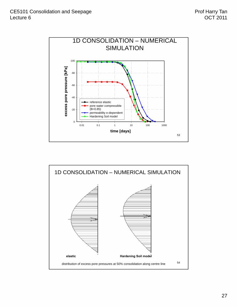
1D CONSOLIDATION – NUMERICAL SIMULATION
kPa]
-100
80
ss p
ore
pre
ssu
re [
k -80
-60
-40
reference elasticpore water compressible
53time [days]
0.01 0.1 1 10 100 1000
exce
s
-20
0
p p(B=0.85)permeability e-dependentHardening Soil model
1D CONSOLIDATION – NUMERICAL SIMULATION
54distribution of excess pore pressures at 50% consolidation along centre line
elastic Hardening Soil model
CE5101 Consolidation and SeepageLecture 6
Prof Harry TanOCT 2011
28
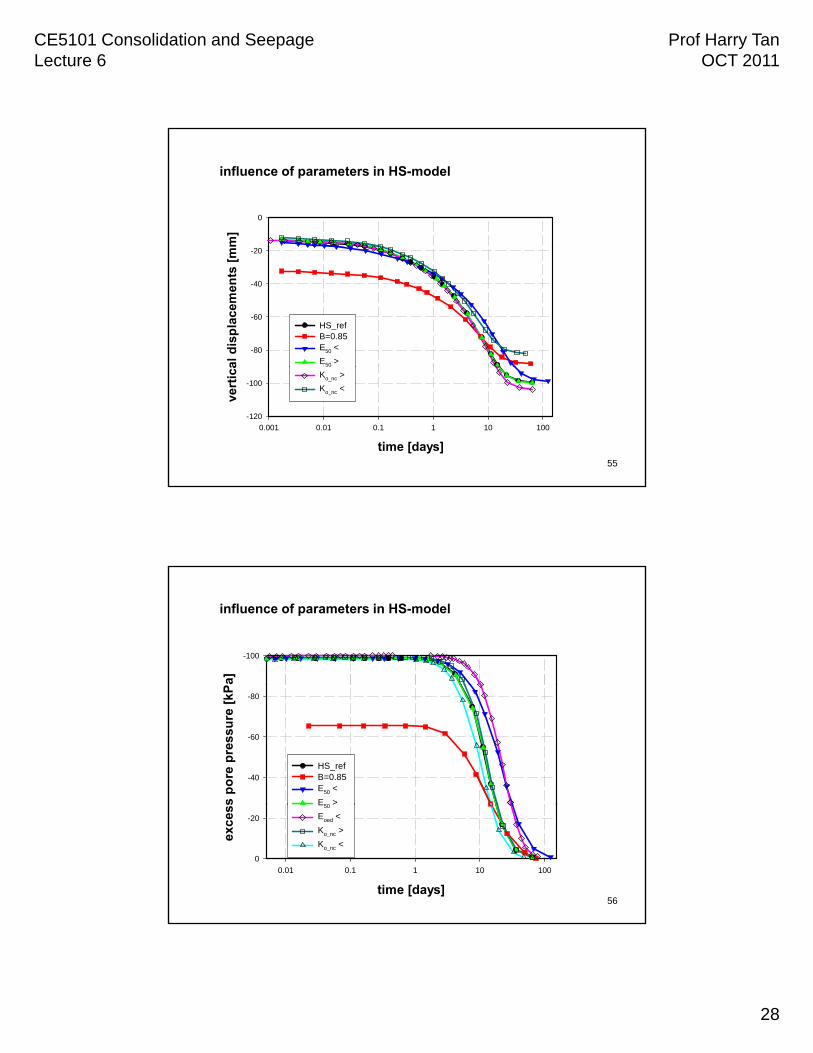
influence of parameters in HS-model
m]
0
al d
isp
lace
men
ts [
m
-80
-60
-40
-20
HS_ref B=0.85E50 <
E50 >
55
time [days]
0.001 0.01 0.1 1 10 100
vert
ica
-120
-100Ko_nc >
Ko_nc <
influence of parameters in HS-model
a]
-100
s p
ore
pre
ssu
re [
kP -80
-60
-40
HS_ref B=0.85E50 <
E50 >
56time [days]
0.01 0.1 1 10 100
exce
ss
-20
0
E50
Eoed <
Ko_nc >
Ko_nc <
CE5101 Consolidation and SeepageLecture 6
Prof Harry TanOCT 2011
29
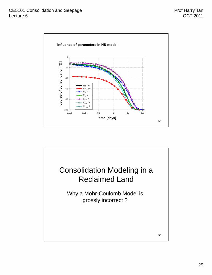
influence of parameters in HS-model
%]
0
e o
f co
nso
lid
atio
n [
%
20
40
60
HS_ref B=0.85E50 <
E50 >
57time [days]
0.001 0.01 0.1 1 10 100
deg
ree
80
100
50
Eoed >
Ko_nc >
Ko_nc <
Consolidation Modeling in a Reclaimed LandReclaimed Land
Why a Mohr-Coulomb Model is grossly incorrect ?
58
CE5101 Consolidation and SeepageLecture 6
Prof Harry TanOCT 2011
30
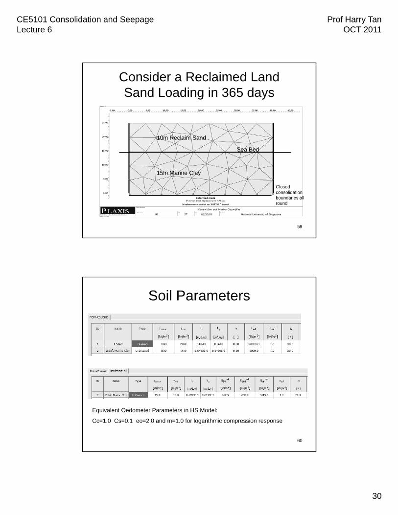
Consider a Reclaimed LandSand Loading in 365 days
10m Reclaim Sand
15m Marine Clay
Sea Bed
59
Closed consolidation boundaries all round
Soil Parameters
60
Equivalent Oedometer Parameters in HS Model:
Cc=1.0 Cs=0.1 eo=2.0 and m=1.0 for logarithmic compression response
CE5101 Consolidation and SeepageLecture 6
Prof Harry TanOCT 2011
31
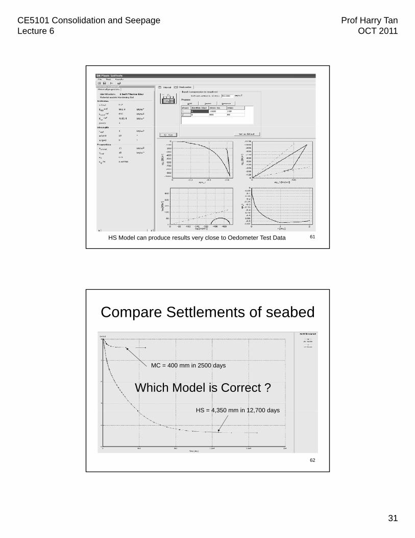
61HS Model can produce results very close to Oedometer Test Data
Compare Settlements of seabed
MC = 400 mm in 2500 days
HS = 4 350 mm in 12 700 days
Which Model is Correct ?
62
HS 4,350 mm in 12,700 days
CE5101 Consolidation and SeepageLecture 6
Prof Harry TanOCT 2011
32
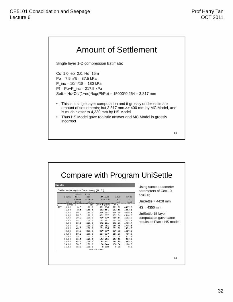
Amount of Settlement
Single layer 1-D compression Estimate:
Cc=1.0, eo=2.0, Ho=15mPo = 7.5m*5 = 37.5 kPaP_inc = 10m*18 = 180 kPaPf = Po+P_inc = 217.5 kPaSett = Ho*Cc/(1+eo)*log(Pf/Po) = 15000*0.254 = 3,817 mm
• This is a single layer computation and it grossly under-estimate
63
g y p g yamount of settlements; but 3,817 mm >> 400 mm by MC Model, and is much closer to 4,330 mm by HS Model
• Thus HS Model gave realistic answer and MC Model is grossly incorrect
Compare with Program UniSettle Using same oedometer parameters of Cc=1.0, eo=2.0;;
UniSettle = 4428 mm
HS = 4350 mm
UniSettle 15-layer computation gave same results as Plaxis HS model
64
CE5101 Consolidation and SeepageLecture 6
Prof Harry TanOCT 2011
33
Conclusions
• MC Model cannot be used for consolidation analysis of soft soilsanalysis of soft soils
• The linear elastic model in MC cannot predict both the rate and amount of consolidation settlements of highly nonlinear soft clays
• The HS Model with equivalent oedometer parameters will give very good predictions of
65
parameters will give very good predictions of both rate and amount of consolidation settlements
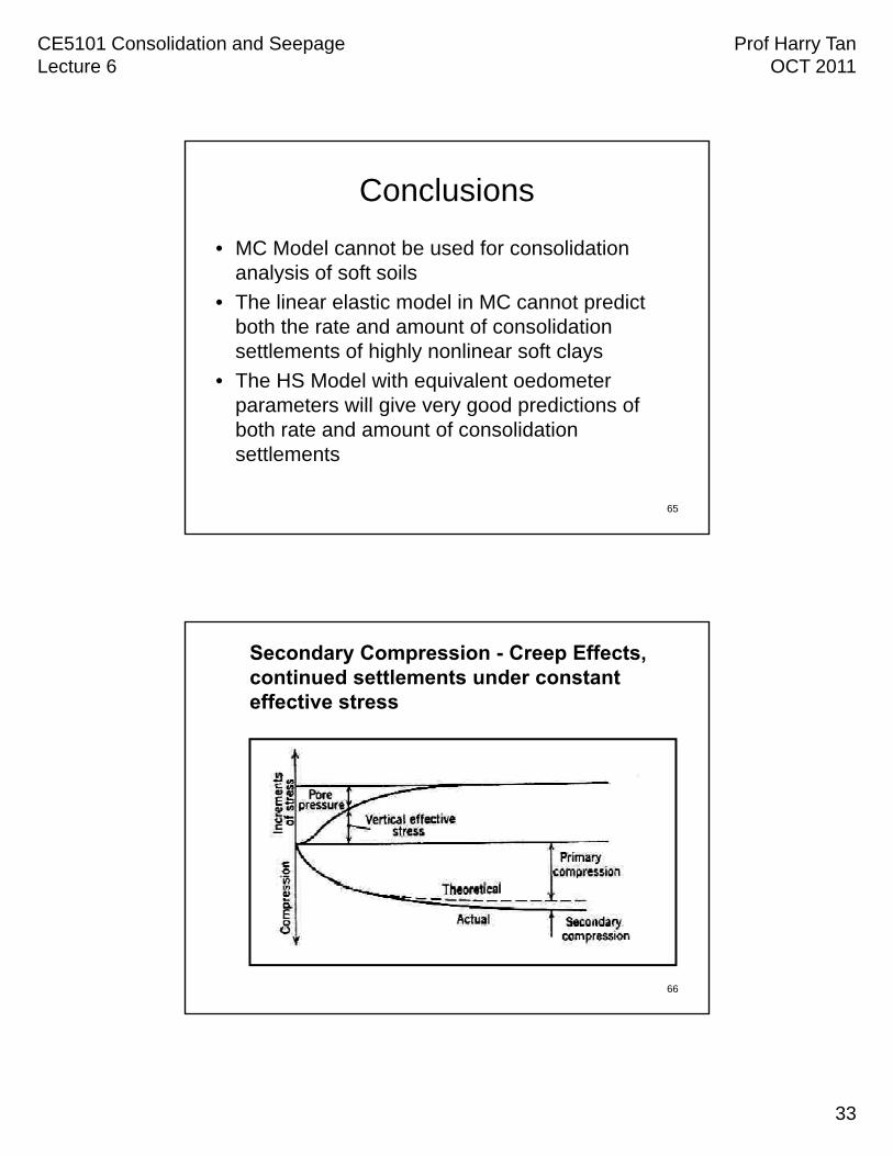
Secondary Compression - Creep Effects, continued settlements under constant effective stress
66
CE5101 Consolidation and SeepageLecture 6
Prof Harry TanOCT 2011
34
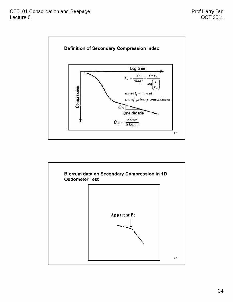
Definition of Secondary Compression Index
ionconsolidatprimary of end
at timetwhere
t
tlog
ee
tlog
eC
p
p
p
67
Bjerrum data on Secondary Compression in 1D Oedometer Test
Apparent Pc
68
CE5101 Consolidation and SeepageLecture 6
Prof Harry TanOCT 2011
35
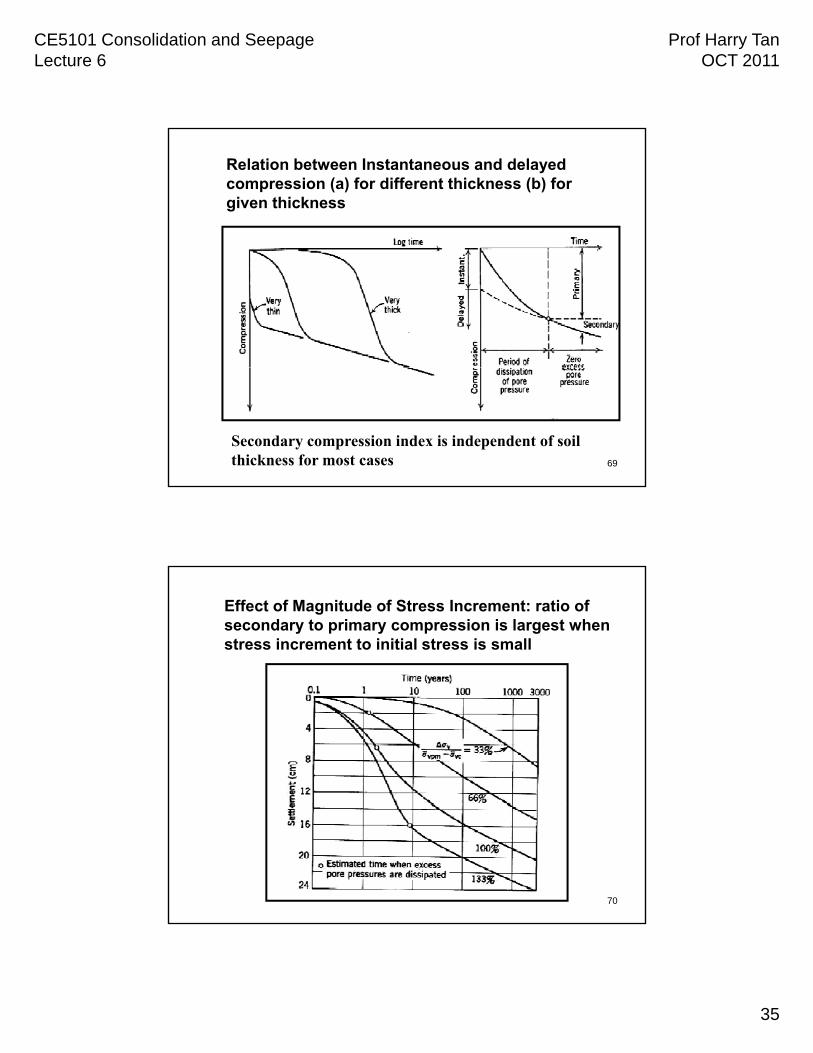
Relation between Instantaneous and delayed compression (a) for different thickness (b) for given thickness
69
Secondary compression index is independent of soil thickness for most cases
Effect of Magnitude of Stress Increment: ratio of secondary to primary compression is largest when stress increment to initial stress is small
70
CE5101 Consolidation and SeepageLecture 6
Prof Harry TanOCT 2011
36
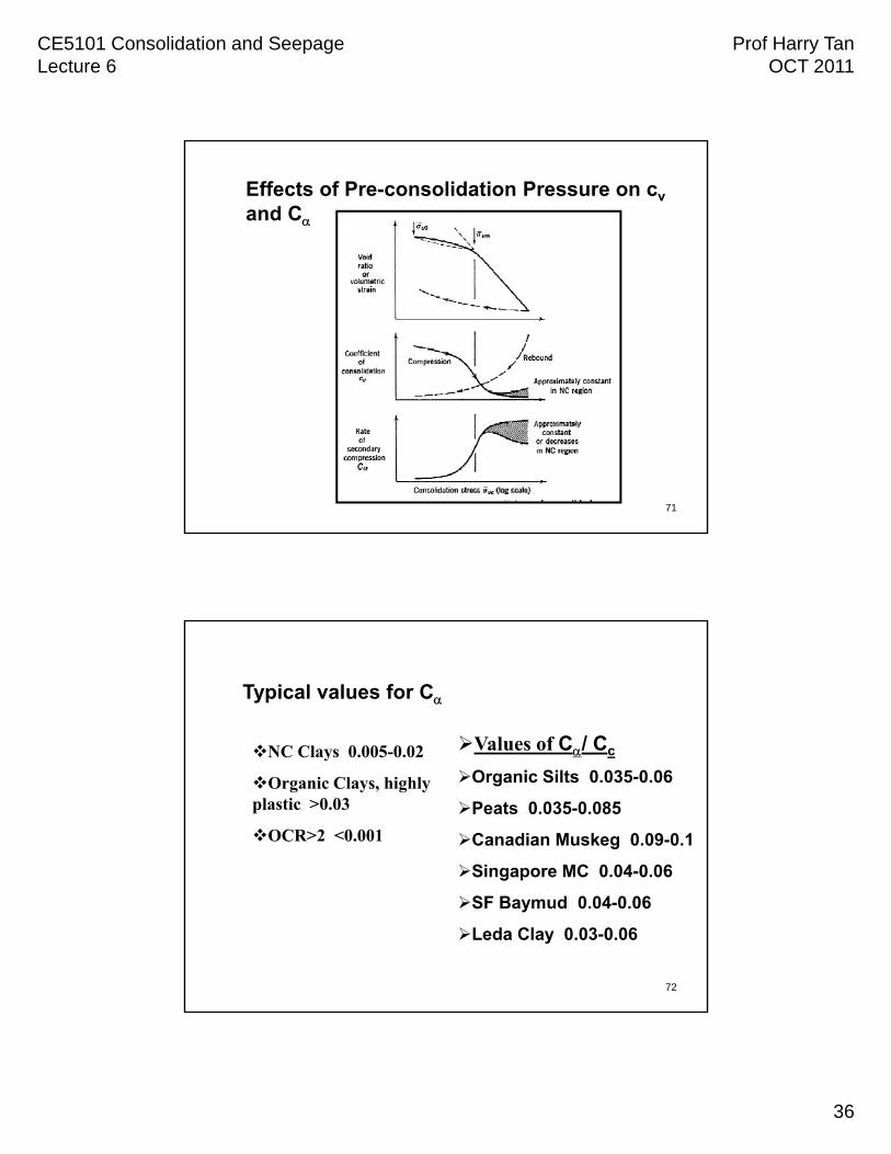
Effects of Pre-consolidation Pressure on cv
and C
71
Typical values for C
NC Clays 0 005 0 02 Values of C/ CcNC Clays 0.005-0.02
Organic Clays, highly plastic >0.03
OCR>2 <0.001
c
Organic Silts 0.035-0.06
Peats 0.035-0.085
Canadian Muskeg 0.09-0.1
Singapore MC 0.04-0.06
72
SF Baymud 0.04-0.06
Leda Clay 0.03-0.06
CE5101 Consolidation and SeepageLecture 6
Prof Harry TanOCT 2011
37
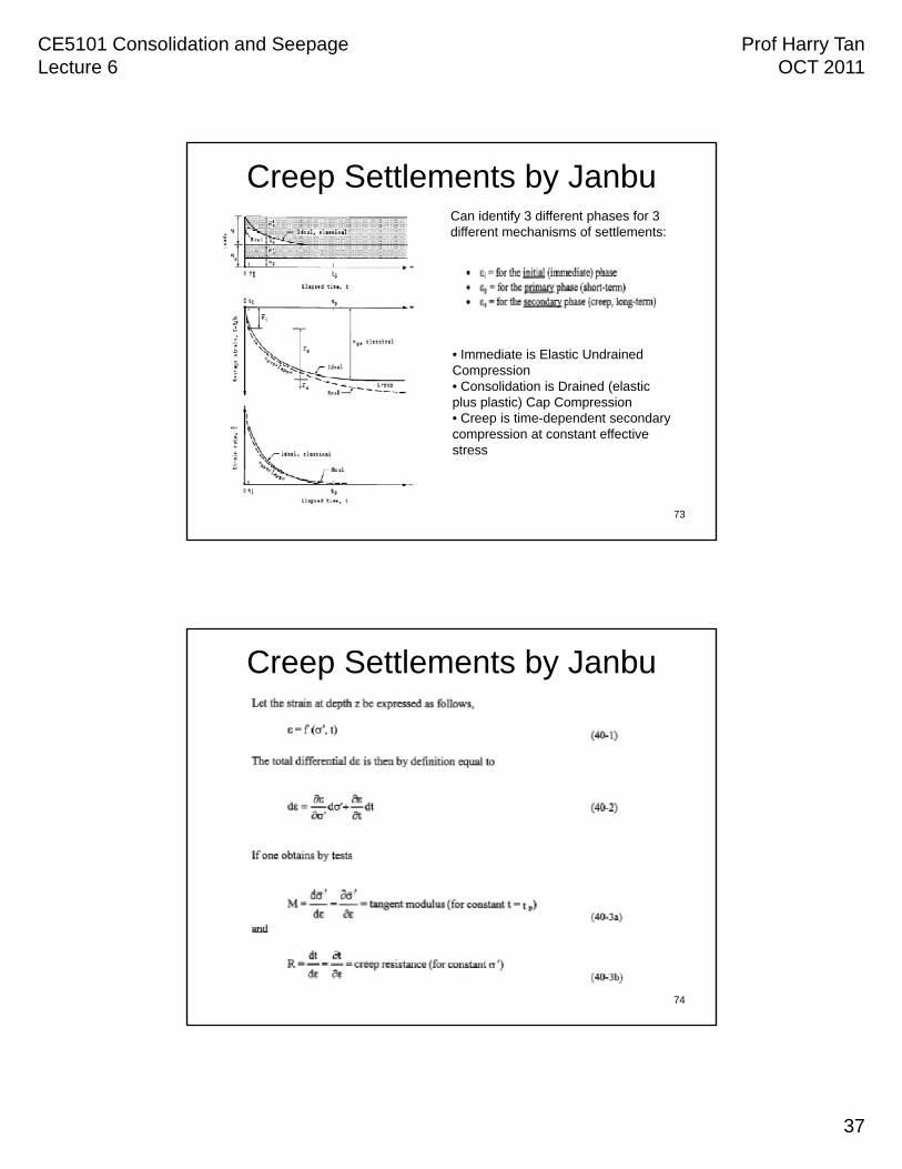
Creep Settlements by JanbuCan identify 3 different phases for 3 different mechanisms of settlements:
• Immediate is Elastic Undrained Compression• Consolidation is Drained (elastic plus plastic) Cap Compression
73
p p ) p p• Creep is time-dependent secondary compression at constant effective stress
Creep Settlements by Janbu
74
CE5101 Consolidation and SeepageLecture 6
Prof Harry TanOCT 2011
38
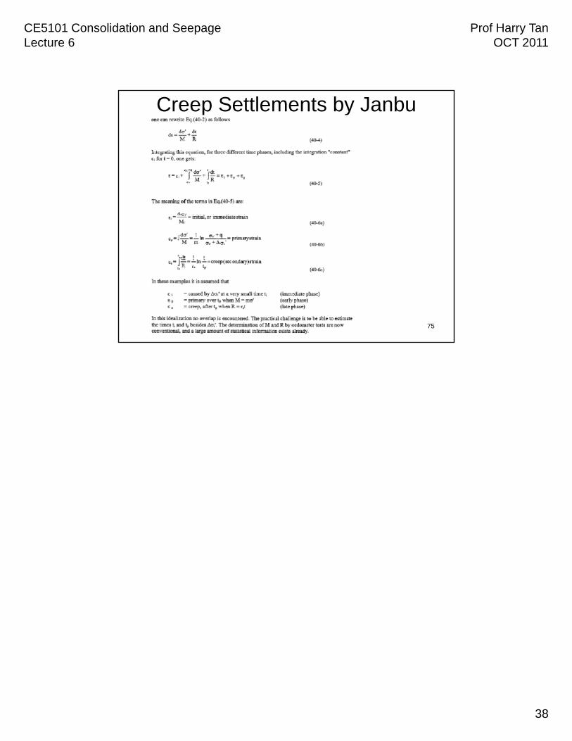
Creep Settlements by Janbu
75