Embed Size (px)
Citation preview

2-1
TSM Base Case Algorithms
State Estimation-Abhimanyu Gartia, WRLDC
2-2
SE Problem Development
What’s A State?– The complete “solution” of the power system is
known if all voltages and angles are identified at each bus. These quantities are the “state variables” of the system.
– Why Estimate?– Meters aren’t perfect.– Meters aren’t everywhere.– Very few phase measurements?– SE suppresses bad measurements and uses the
measurement set to the fullest extent.
2-3
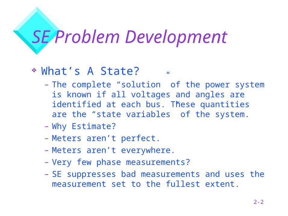
SE Problem Development (Cont.)
Mathematically Speaking...Z = [ h( x ) + e ]
where,Z = Measurement Vectorh = System Model relating state vector to the measurement setx = State Vector (voltage magnitudes and angles)e = Error Vector associated with the measurement set
2-4
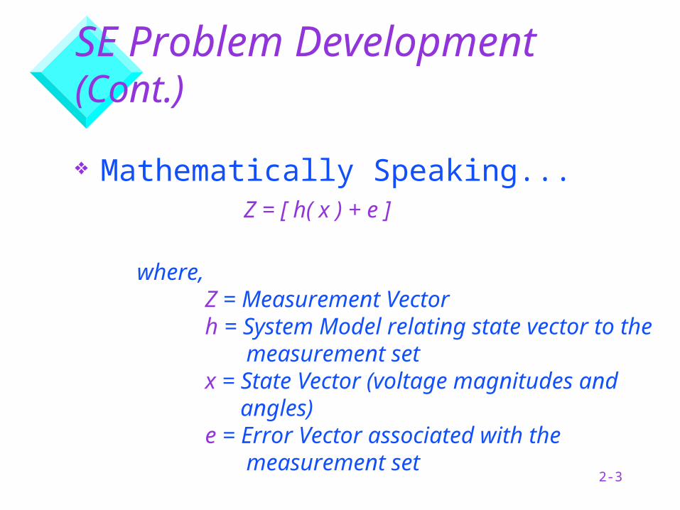
SE Problem Development (Cont.)
Linearizing…
Classical Approach -> Weighted Least Squares…
Z = H x + e
(This looks like a load flow equation )
Minimize: J(x) = [z - h(x)] t. W. [z - h(x)] where,
J = Weighted least squares matrixW = Error covariance matrix
2-5
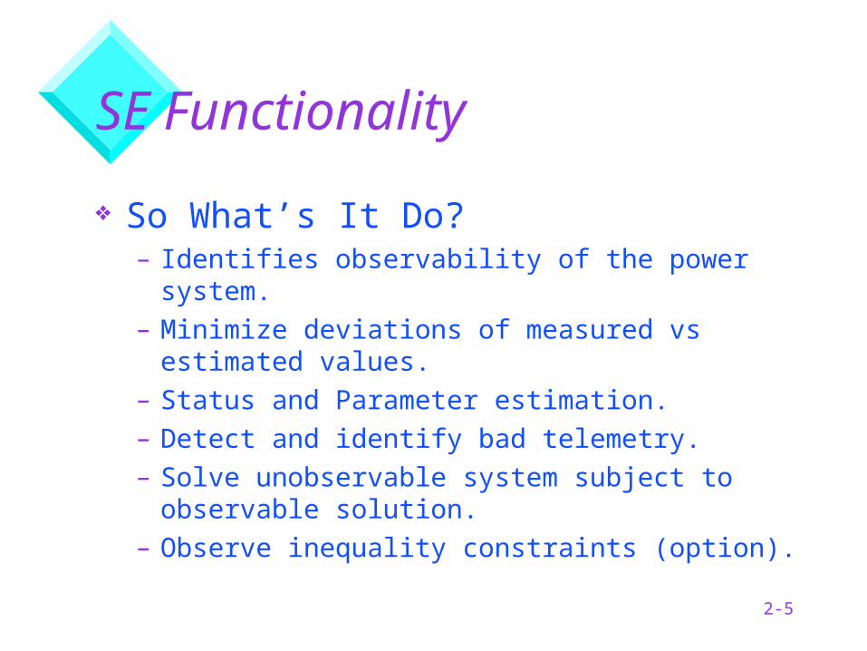
SE Functionality
So What’s It Do?– Identifies observability of the power system.– Minimize deviations of measured vs
estimated values.– Status and Parameter estimation.– Detect and identify bad telemetry.– Solve unobservable system subject to
observable solution.– Observe inequality constraints (option).
2-6
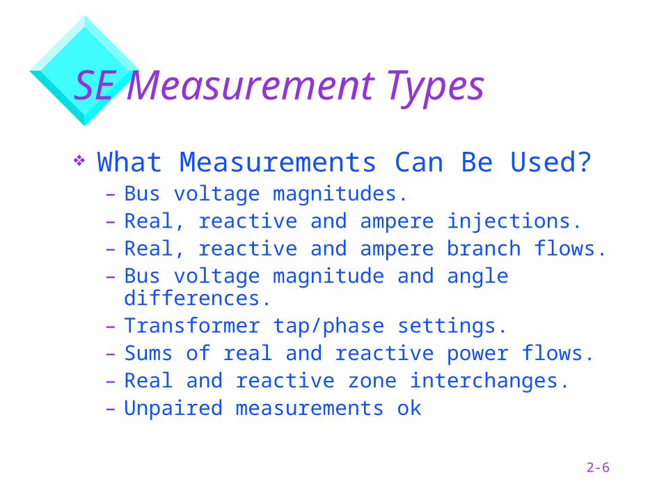
SE Measurement Types
What Measurements Can Be Used?– Bus voltage magnitudes.– Real, reactive and ampere injections.– Real, reactive and ampere branch flows.– Bus voltage magnitude and angle
differences.– Transformer tap/phase settings.– Sums of real and reactive power flows.– Real and reactive zone interchanges.– Unpaired measurements ok
2-7
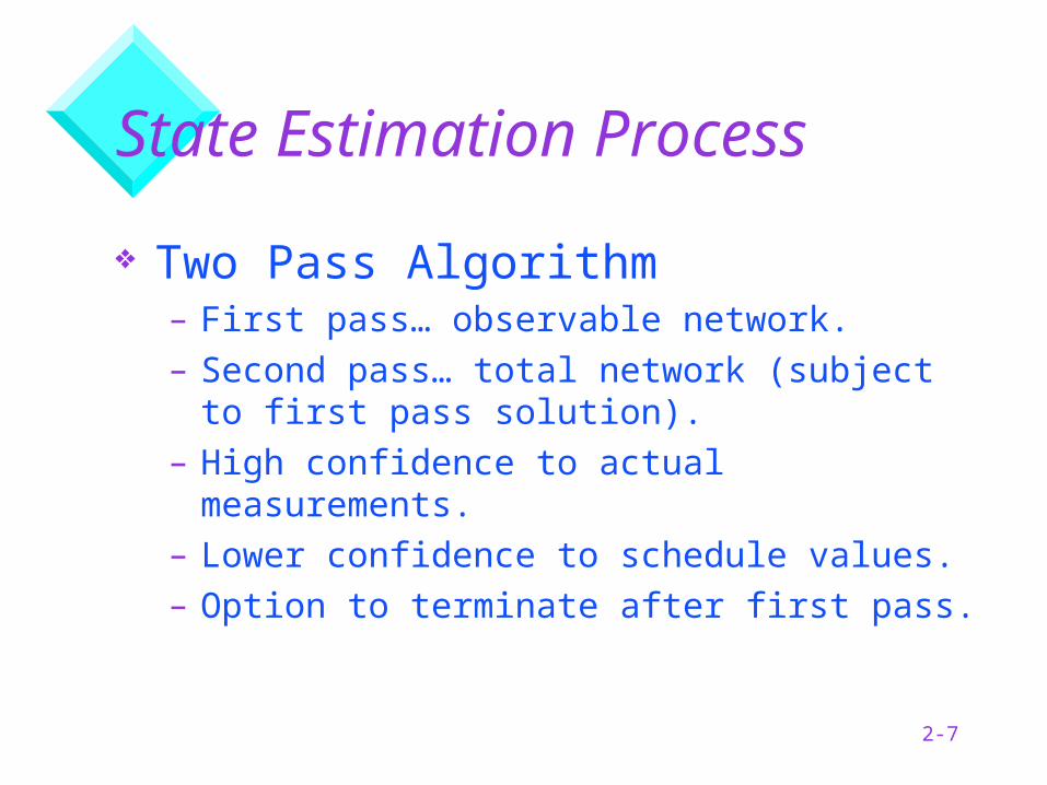
State Estimation Process
Two Pass Algorithm– First pass… observable network.– Second pass… total network (subject to first
pass solution).– High confidence to actual measurements.– Lower confidence to schedule values.– Option to terminate after first pass.
2-8
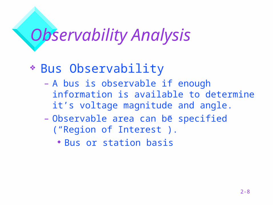
Observability Analysis
Bus Observability– A bus is observable if enough information is
available to determine it’s voltage magnitude and angle.
– Observable area can be specified (“Region of Interest”).
Bus or station basis
2-9
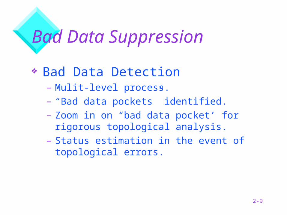
Bad Data Suppression
Bad Data Detection– Mulit-level process.– “Bad data pockets” identified.– Zoom in on “bad data pocket’ for rigorous
topological analysis.– Status estimation in the event of
topological errors.
2-10
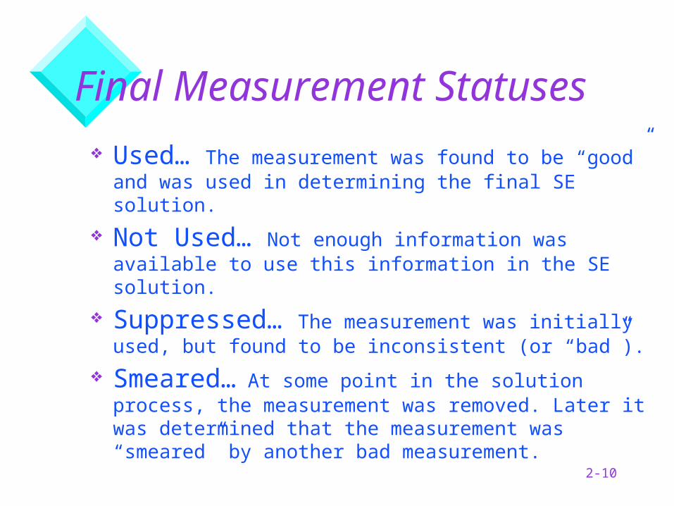
Final Measurement Statuses
Used… The measurement was found to be “good” and was used in determining the final SE solution.
Not Used… Not enough information was available to use this information in the SE solution.
Suppressed… The measurement was initially used, but found to be inconsistent (or “bad”).
Smeared… At some point in the solution process, the measurement was removed. Later it was determined that the measurement was “smeared” by another bad measurement.
2-11
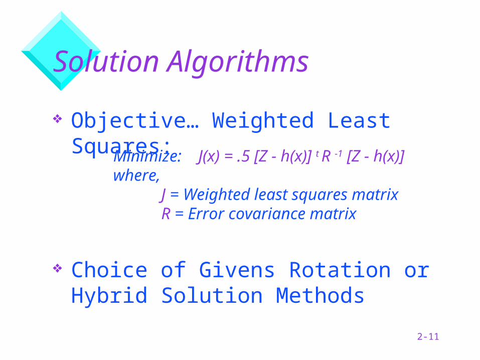
Solution Algorithms
Objective… Weighted Least Squares:
Choice of Givens Rotation or Hybrid Solution Methods
Minimize: J(x) = .5 [Z - h(x)] t R -1 [Z - h(x)]where,
J = Weighted least squares matrixR = Error covariance matrix
2-12
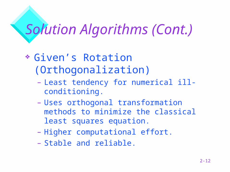
Solution Algorithms (Cont.)
Given’s Rotation (Orthogonalization)– Least tendency for numerical ill-
conditioning. – Uses orthogonal transformation methods to
minimize the classical least squares equation.
– Higher computational effort.– Stable and reliable.
2-13
SE Problem Development (Cont.)
Hybrid Approach– Mixture of Normal Equations and
Orthogonalization.– Orthogonalization uses a fast Given’s
rotation for numerical robustness.– Normal Equations used for solution state
updates which minimizes storage requirements.
– Stable, reliable and efficient.
2-14
SE Program Constants
Please Refer To Real-Time Program Constants Display.
2-15
Base Case Algorithms
Power Flow
2-16
PF Problem Development
Purpose– Solve the general network consisting of all
voltages and branches flows.
How PF Differs From SE– Unlike the SE algorithm, PF does not have
to contend with measurement inconsistencies (I.e., branch flows are not inputs to the algorithm).
– PF has no concept of “observability”.
2-17
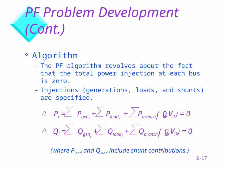
PF Problem Development (Cont.)
Algorithm– The PF algorithm revolves about the fact that
the total power injection at each bus is zero.– Injections (generations, loads, and shunts)
are specified.
Pi = Pgeni + Ploadi
+ Pbranchi( ik,Vik) = 00
Qi = Qgeni + Qloadi
+ Qbranchi( ik,Vik) = 00
(where Pload and Qload include shunt contributions.)
2-18
V
Fully Coupled Power Flow
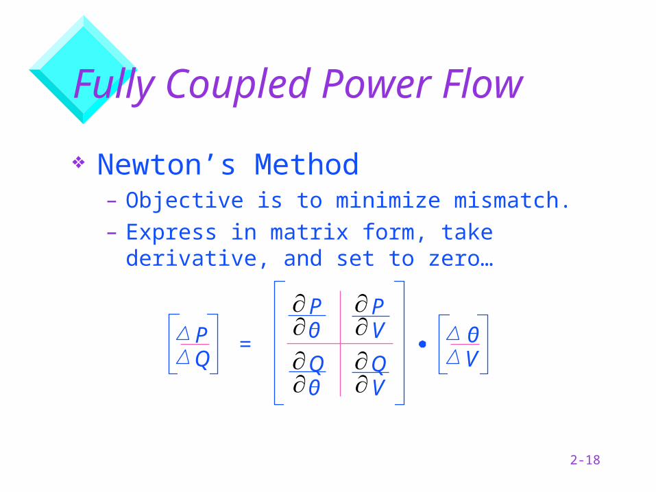
Newton’s Method– Objective is to minimize mismatch.– Express in matrix form, take derivative, and
set to zero…
PQ
P0
P
VQ0
Q
V0=
2-19
Fast Decoupled Power Flow
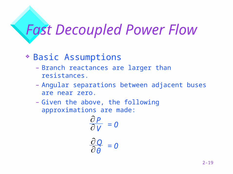
Basic Assumptions– Branch reactances are larger than resistances.– Angular separations between adjacent buses
are near zero.– Given the above, the following approximations
are made:
VP
Q0
= 0
= 0
2-20
Fast Decoupled Power Flow (Cont.)
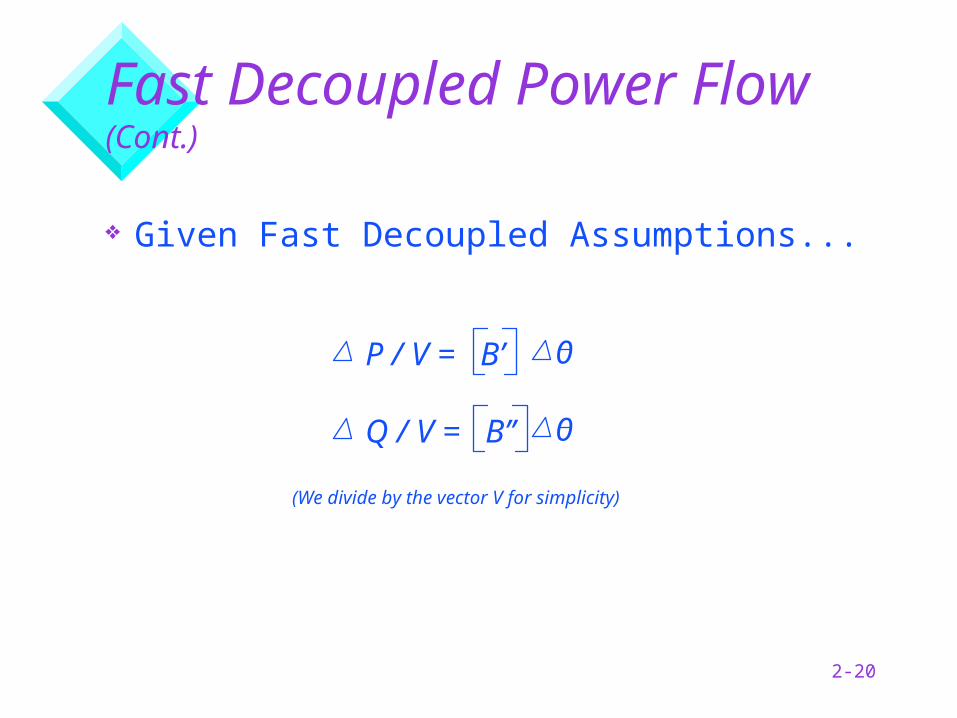
Given Fast Decoupled Assumptions...
P / V = B’ 0
Q / V = B’’ 0
(We divide by the vector V for simplicity)
2-21
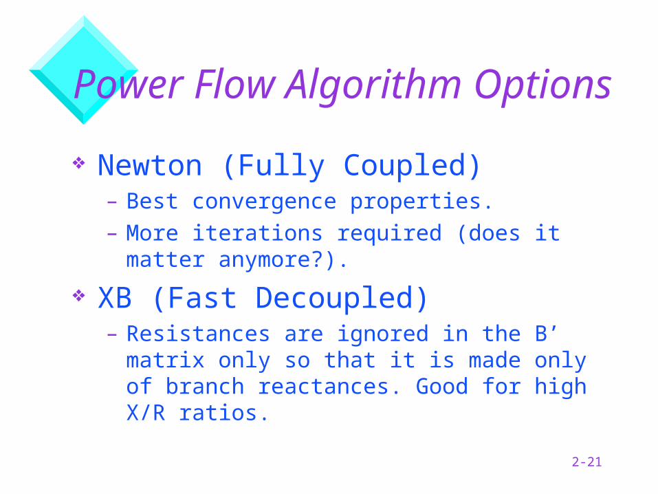
Power Flow Algorithm Options
Newton (Fully Coupled)– Best convergence properties.– More iterations required (does it matter
anymore?).
XB (Fast Decoupled)– Resistances are ignored in the B’ matrix
only so that it is made only of branch reactances. Good for high X/R ratios.
2-22
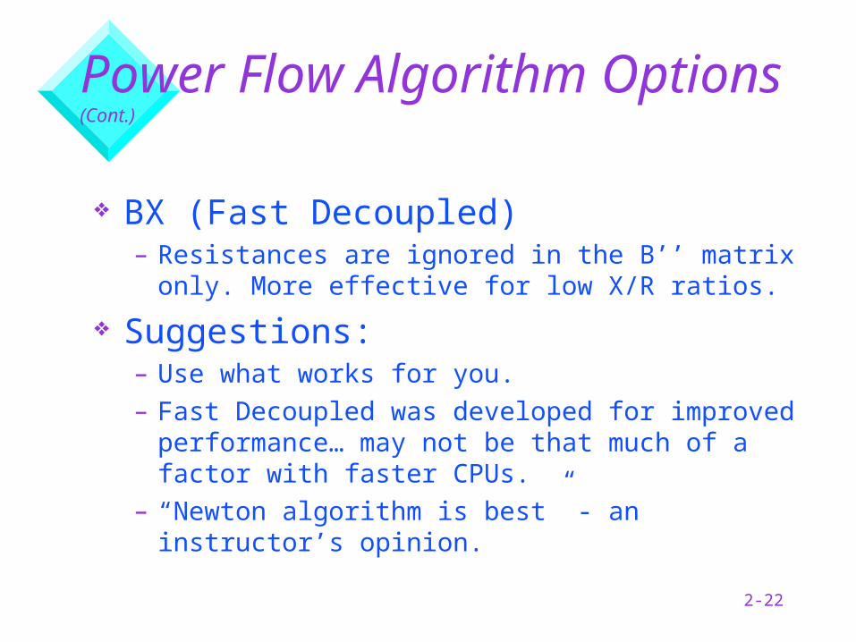
Power Flow Algorithm Options (Cont.)
BX (Fast Decoupled)– Resistances are ignored in the B’’ matrix
only. More effective for low X/R ratios.
Suggestions:– Use what works for you.– Fast Decoupled was developed for improved
performance… may not be that much of a factor with faster CPUs.
– “Newton algorithm is best” - an instructor’s opinion.
2-23
GENS Implementations
Running The Applications &
Interpreting Results
2-24
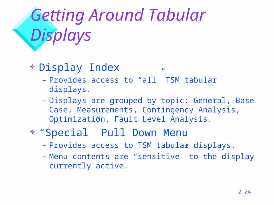
Getting Around Tabular Displays
Display Index– Provides access to “all” TSM tabular displays.– Displays are grouped by topic: General, Base
Case, Measurements, Contingency Analysis, Optimization, Fault Level Analysis.
“Special” Pull Down Menu– Provides access to TSM tabular displays.– Menu contents are “sensitive” to the display
currently active.
2-25
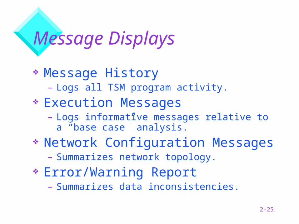
Message Displays
Message History– Logs all TSM program activity.
Execution Messages– Logs informative messages relative to a
“base case” analysis. Network Configuration Messages
– Summarizes network topology. Error/Warning Report
– Summarizes data inconsistencies.
2-26
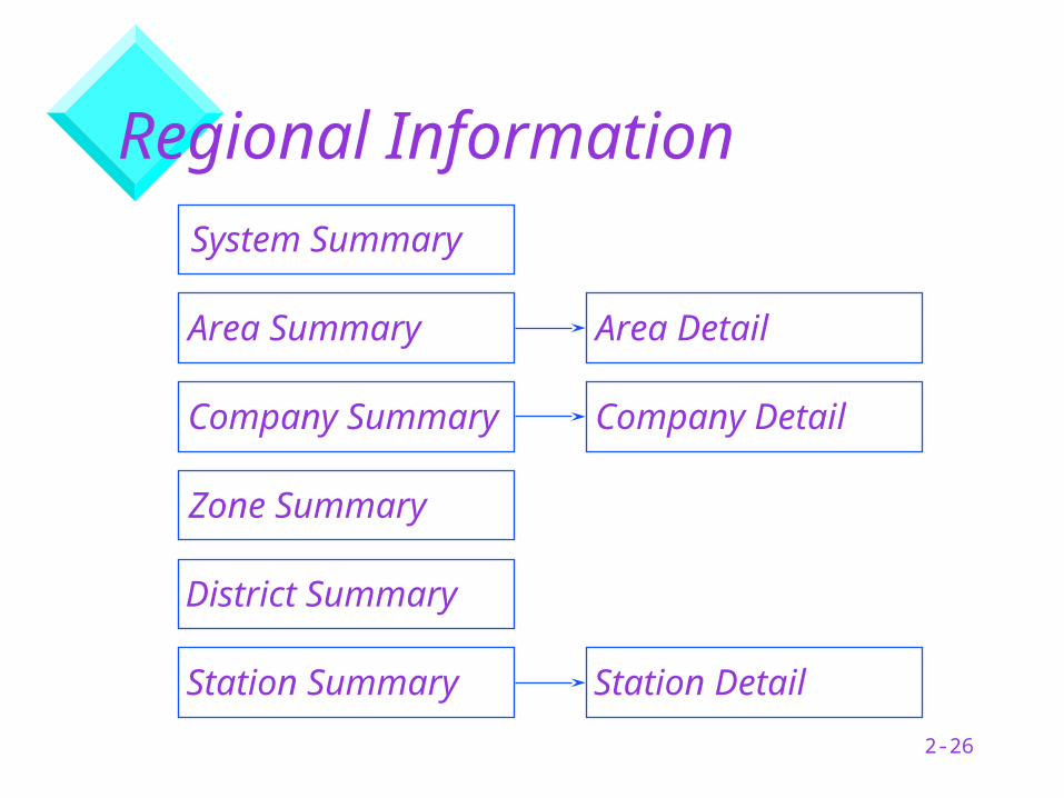
Regional InformationSystem Summary
Area Summary
Company Summary
Zone Summary
District Summary
Station Summary
Area Detail
Company Detail
Station Detail
2-27
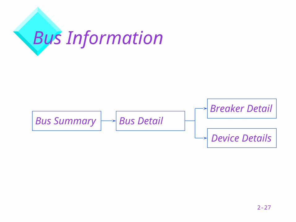
Bus Information
Bus Summary Bus DetailBreaker Detail
Device Details
2-28
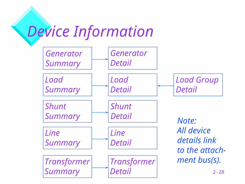
Device InformationGenerator Summary
LoadSummary
ShuntSummary
LineSummary
TransformerSummary
GeneratorDetail
LoadDetail
ShuntDetail
LineDetail
TransformerDetail
Load GroupDetail
Note:All devicedetails linkto the attach-ment bus(s).
2-29
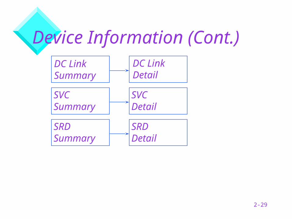
Device Information (Cont.)DC Link Summary
SVCSummary
SRDSummary
DC LinkDetail
SVCDetail
SRDDetail
2-30
Displaying Results On One-Lines
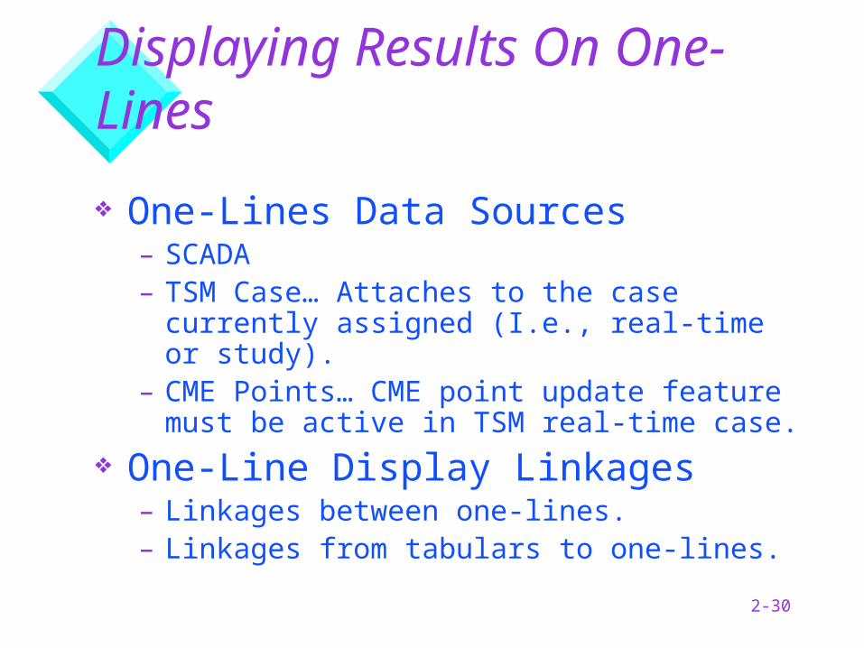
One-Lines Data Sources– SCADA– TSM Case… Attaches to the case currently
assigned (I.e., real-time or study).– CME Points… CME point update feature
must be active in TSM real-time case. One-Line Display Linkages
– Linkages between one-lines.– Linkages from tabulars to one-lines.
2-31
TSM Constraints
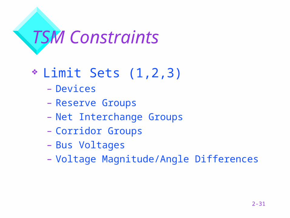
Limit Sets (1,2,3)– Devices– Reserve Groups– Net Interchange Groups– Corridor Groups– Bus Voltages– Voltage Magnitude/Angle Differences
2-32
TSM Constraints (Cont.)
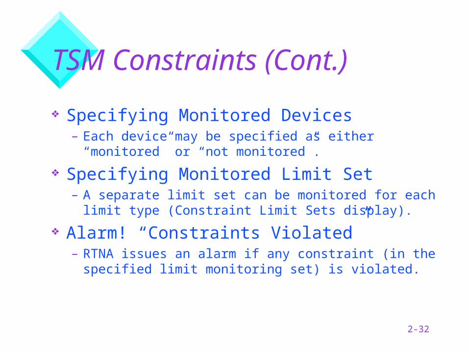
Specifying Monitored Devices– Each device may be specified as either
“monitored” or “not monitored”.
Specifying Monitored Limit Set– A separate limit set can be monitored for
each limit type (Constraint Limit Sets display).
Alarm! “Constraints Violated”– RTNA issues an alarm if any constraint (in the
specified limit monitoring set) is violated.
2-33
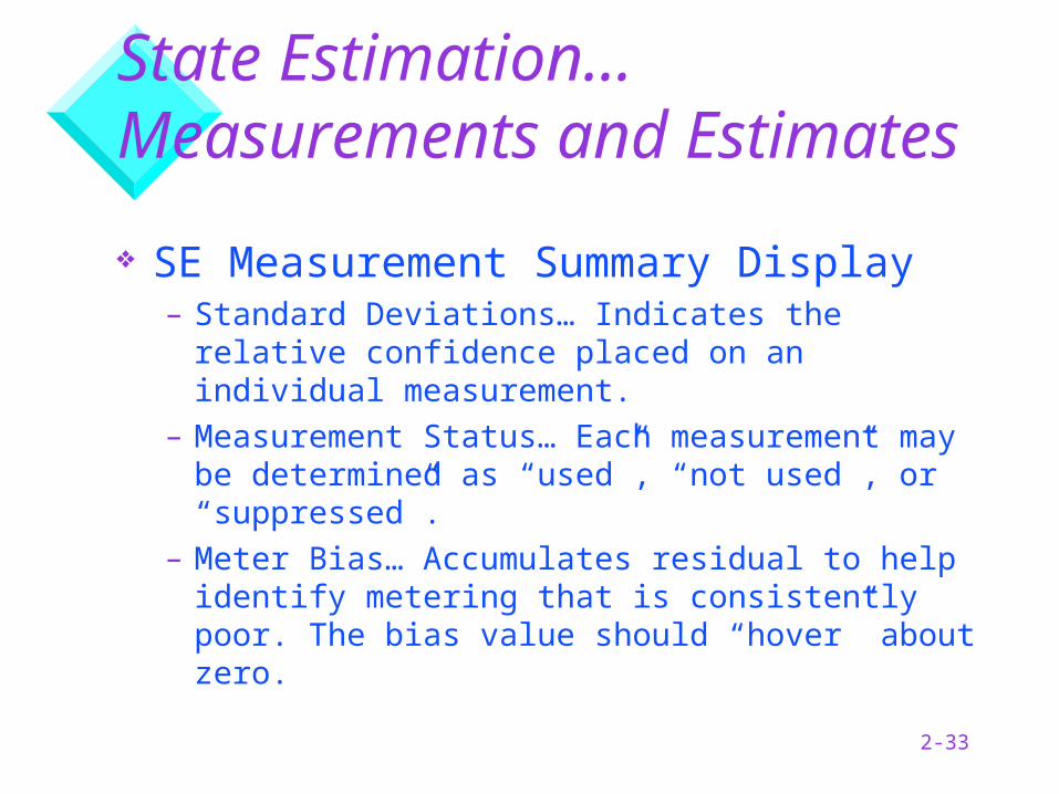
State Estimation...Measurements and Estimates
SE Measurement Summary Display– Standard Deviations… Indicates the relative
confidence placed on an individual measurement.
– Measurement Status… Each measurement may be determined as “used”, “not used”, or “suppressed”.
– Meter Bias… Accumulates residual to help identify metering that is consistently poor. The bias value should “hover” about zero.

2-34
State Estimation...Measurements and Estimates (Cont.)
Suppressed Measurement Summary Display– SE will suppress measurements it feels are
inconsistent with the other system measurements.
10 9.5
3.7
15.2NOPE!
2-35
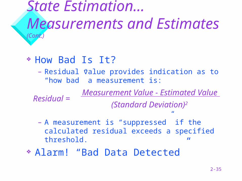
State Estimation...Measurements and Estimates (Cont.)
How Bad Is It?– Residual value provides indication as to “how
bad” a measurement is:
– A measurement is “suppressed” if the calculated residual exceeds a specified threshold.
Alarm! “Bad Data Detected”
Residual = Measurement Value - Estimated Value
(Standard Deviation)2
2-36
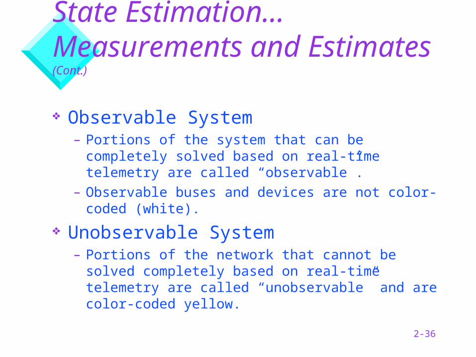
State Estimation...Measurements and Estimates (Cont.)
Observable System– Portions of the system that can be completely
solved based on real-time telemetry are called “observable”.
– Observable buses and devices are not color-coded (white).
Unobservable System– Portions of the network that cannot be solved
completely based on real-time telemetry are called “unobservable” and are color-coded yellow.
2-37
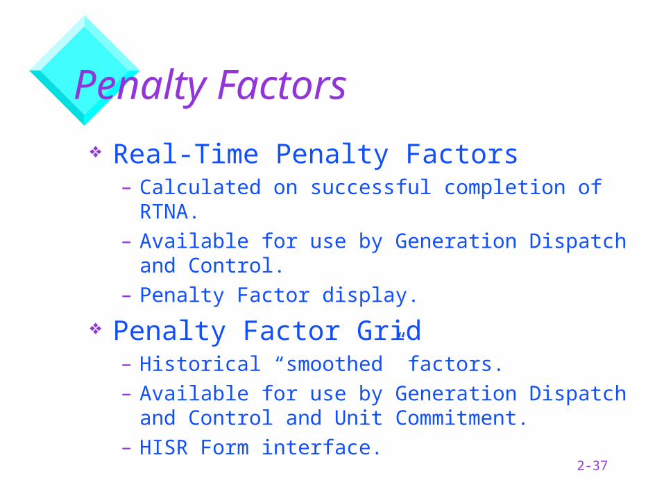
Penalty Factors
Real-Time Penalty Factors– Calculated on successful completion of RTNA.– Available for use by Generation Dispatch and
Control.– Penalty Factor display.
Penalty Factor Grid– Historical “smoothed” factors.– Available for use by Generation Dispatch and
Control and Unit Commitment.– HISR Form interface.

2-38
Study Applications
Be Free…You can’t hurt
anything
2-39
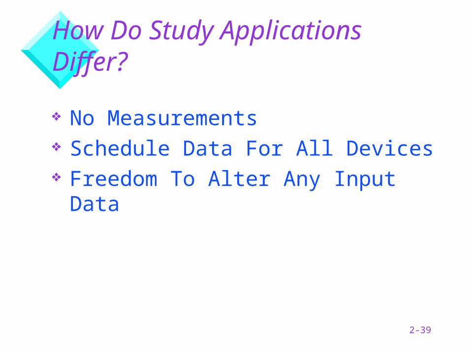
How Do Study Applications Differ?
No Measurements Schedule Data For All Devices Freedom To Alter Any Input Data
2-40
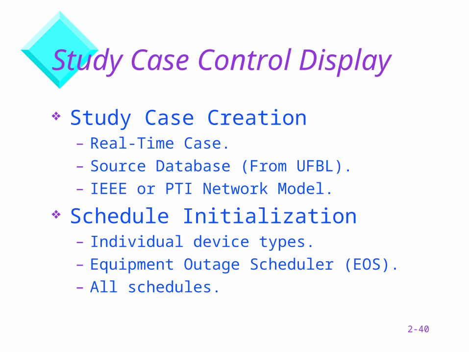
Study Case Control Display
Study Case Creation– Real-Time Case.– Source Database (From UFBL).– IEEE or PTI Network Model.
Schedule Initialization– Individual device types.– Equipment Outage Scheduler (EOS).– All schedules.
2-41
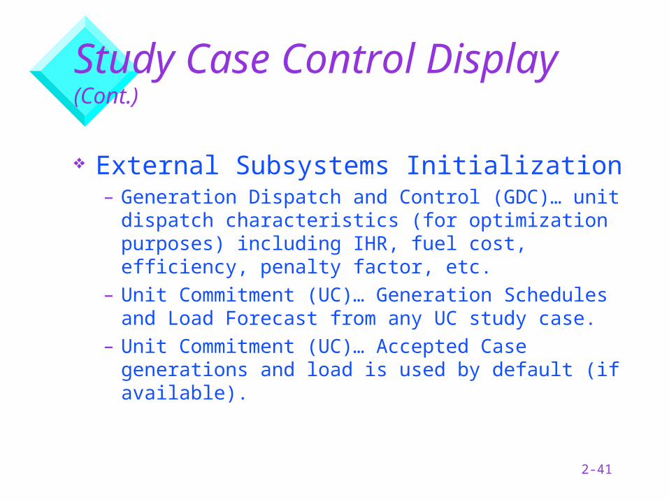
Study Case Control Display (Cont.)
External Subsystems Initialization– Generation Dispatch and Control (GDC)… unit
dispatch characteristics (for optimization purposes) including IHR, fuel cost, efficiency, penalty factor, etc.
– Unit Commitment (UC)… Generation Schedules and Load Forecast from any UC study case.
– Unit Commitment (UC)… Accepted Case generations and load is used by default (if available).
2-42
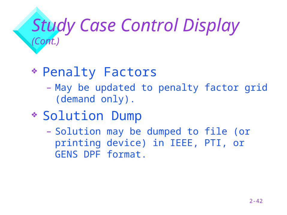
Study Case Control Display (Cont.)
Penalty Factors– May be updated to penalty factor grid
(demand only).
Solution Dump– Solution may be dumped to file (or printing
device) in IEEE, PTI, or GENS DPF format.
2-43
Study Case Control Display (Cont.)
Module Indicators– Same as real-time with the following
exceptions:– NC… Does not retrieve real-time telemetry.
Rather uses predefined switch statuses and device schedules.
– DPF… Replaces SE functionality. Solves the network model and reports violations.
2-44
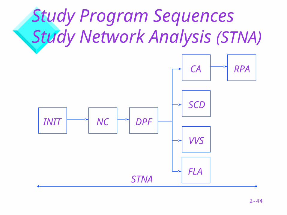
Study Program SequencesStudy Network Analysis (STNA)
INIT NC DPF
CA RPA
SCD
VVS
STNAFLA
2-45
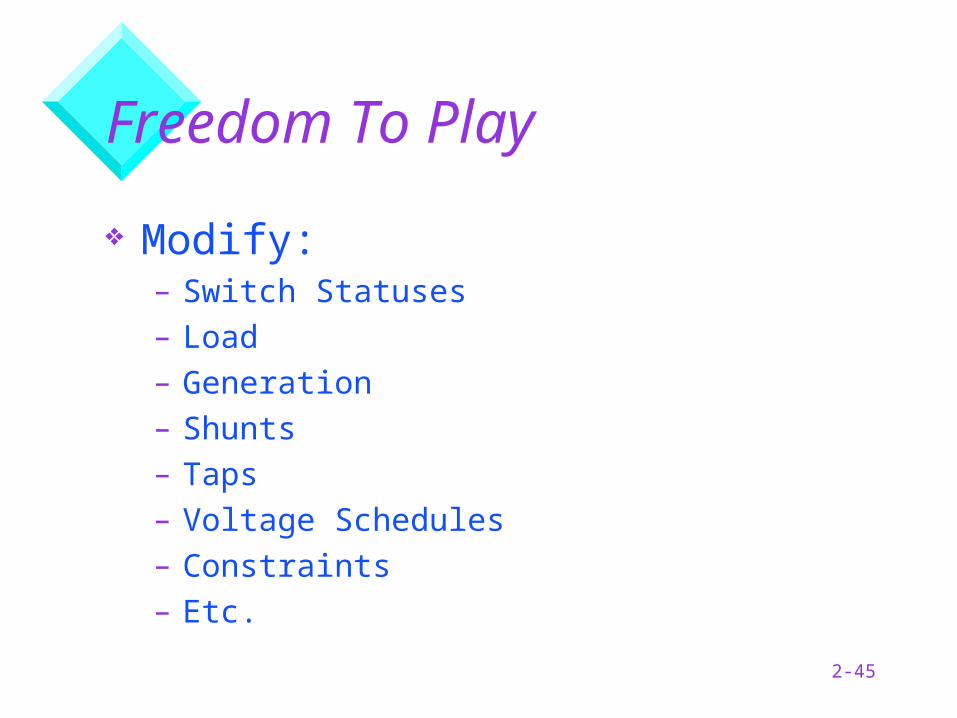
Freedom To Play
Modify:– Switch Statuses– Load– Generation– Shunts– Taps– Voltage Schedules– Constraints– Etc.
2-46
Automatic Control Simulation
Control Options:– Remote voltage control by MVAR
generation.– Local/Remote voltage control by shunts.– Local/Remote voltage control by TCULs.– MVAR flow control by TCULs.– MW flow control by phase shifters.– Area MW interchange control.– Reactive generation limit enforcement.
2-47
Viewing Results
Displays Same As Real-Time– Measurement displays do not apply.
One-Line (MDS) Functionality– Keys off case number assignment.