Embed Size (px)
Citation preview

WEAK NULL SINGULARITIES IN GENERAL RELATIVITY
JONATHAN LUK
Abstract. We construct a class of spacetimes (without symmetry assumptions) satisfyingthe vacuum Einstein equations with singular boundaries on two null hypersurfaces intersect-ing in the future on a 2-sphere. The metric of these spacetimes extends continuously beyondthe singularities while the Christoffel symbols fail to be square integrable in a neighborhoodof any point on the singular boundaries. The construction shows moreover that the singu-larities are stable in a suitable sense. These singularities are stronger than the impulsivegravitational spacetimes considered by Luk-Rodnianski and conjecturally they are presentin the interior of generic black holes arising from gravitational collapse.
Contents
1. Introduction 21.1. Weak Null Singularities and Strong Cosmic Censorship Conjecture 61.2. Comparison with Impulsive Gravitational Waves 81.3. Description of the Main Results 91.4. Main Ideas of the Proof 121.5. Outline of the Paper 152. Basic Setup 162.1. Double Null Foliation 162.2. The Coordinate System 162.3. Equations 172.4. Schematic Notation 203. Norms 214. Construction of Initial Data Set 245. The Preliminary Estimates 275.1. Estimates for Metric Components 275.2. Estimates for Transport Equations 295.3. Sobolev Embedding 305.4. Commutation Formulae 315.5. General Elliptic Estimates for Hodge Systems 326. Estimates for the Ricci Coefficients via Transport Equations 337. Elliptic Estimates for Fourth Derivatives of the Ricci Coefficients 388. Estimates for Curvature 469. Nature of the Singular Boundary 5310. Acknowledgments 59References 59
1
arX
iv:1
311.
4970
v3 [
gr-q
c] 5
Oct
201
7
2 JONATHAN LUK
1. Introduction
In this paper, we study the existence and stability of weak null singularities in generalrelativity without symmetry assumptions. More precisely, a weak null singularity is a singularnull boundary of a spacetime (M, g) solving the Einstein equations
Ricµν −1
2Rgµν = Tµν
such that the Christoffel symbols blow up and are not square integrable while the metricis continuous up to the boundary. This can be interpreted as a terminal singularity of thespacetime as it cannot be made sense of as a weak solution1 to the Einstein equations alongthe singular boundary. While the singularity is sufficiently strong to be terminal, it is atthe same time sufficiently weak such that the metric in an appropriate coordinate system iscontinuous up to the boundary.
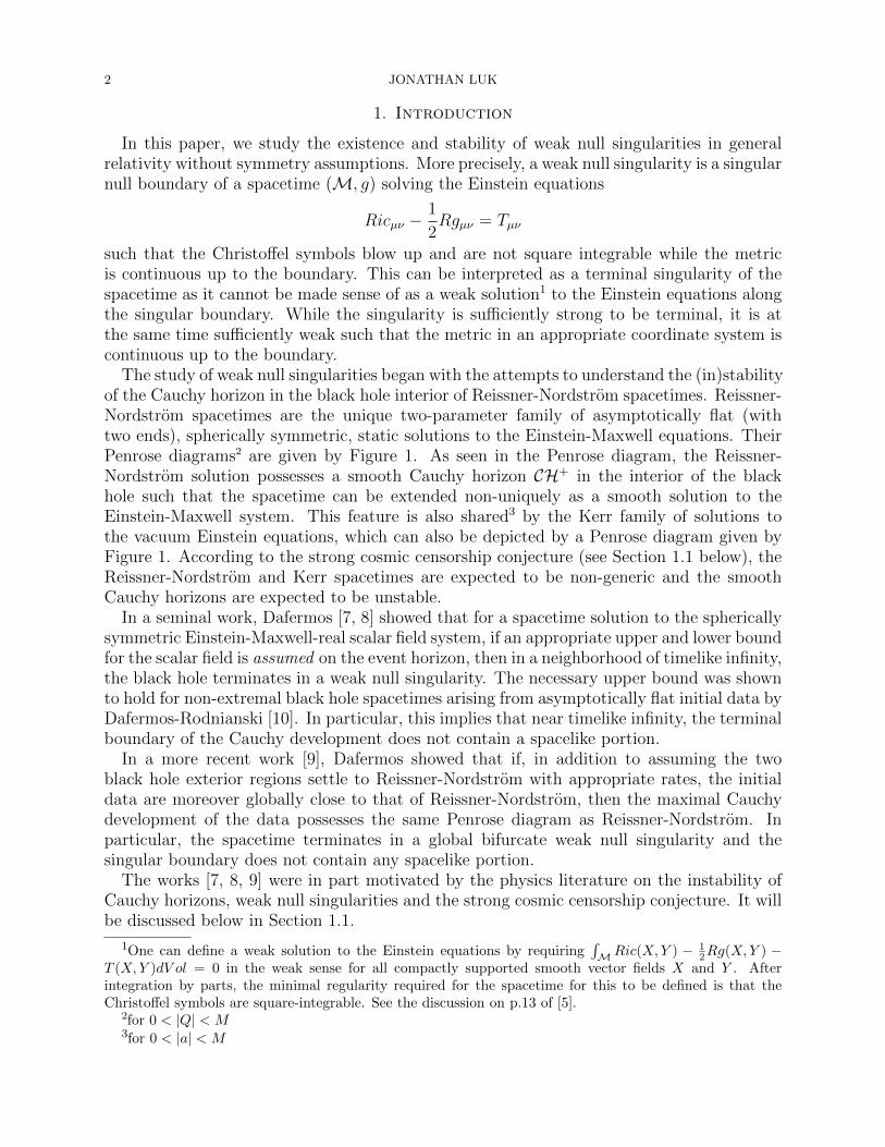
The study of weak null singularities began with the attempts to understand the (in)stabilityof the Cauchy horizon in the black hole interior of Reissner-Nordstrom spacetimes. Reissner-Nordstrom spacetimes are the unique two-parameter family of asymptotically flat (withtwo ends), spherically symmetric, static solutions to the Einstein-Maxwell equations. TheirPenrose diagrams2 are given by Figure 1. As seen in the Penrose diagram, the Reissner-Nordstrom solution possesses a smooth Cauchy horizon CH+ in the interior of the blackhole such that the spacetime can be extended non-uniquely as a smooth solution to theEinstein-Maxwell system. This feature is also shared3 by the Kerr family of solutions tothe vacuum Einstein equations, which can also be depicted by a Penrose diagram given byFigure 1. According to the strong cosmic censorship conjecture (see Section 1.1 below), theReissner-Nordstrom and Kerr spacetimes are expected to be non-generic and the smoothCauchy horizons are expected to be unstable.
In a seminal work, Dafermos [7, 8] showed that for a spacetime solution to the sphericallysymmetric Einstein-Maxwell-real scalar field system, if an appropriate upper and lower boundfor the scalar field is assumed on the event horizon, then in a neighborhood of timelike infinity,the black hole terminates in a weak null singularity. The necessary upper bound was shownto hold for non-extremal black hole spacetimes arising from asymptotically flat initial data byDafermos-Rodnianski [10]. In particular, this implies that near timelike infinity, the terminalboundary of the Cauchy development does not contain a spacelike portion.
In a more recent work [9], Dafermos showed that if, in addition to assuming the twoblack hole exterior regions settle to Reissner-Nordstrom with appropriate rates, the initialdata are moreover globally close to that of Reissner-Nordstrom, then the maximal Cauchydevelopment of the data possesses the same Penrose diagram as Reissner-Nordstrom. Inparticular, the spacetime terminates in a global bifurcate weak null singularity and thesingular boundary does not contain any spacelike portion.
The works [7, 8, 9] were in part motivated by the physics literature on the instability ofCauchy horizons, weak null singularities and the strong cosmic censorship conjecture. It willbe discussed below in Section 1.1.
1One can define a weak solution to the Einstein equations by requiring∫MRic(X,Y ) − 1
2Rg(X,Y ) −T (X,Y )dV ol = 0 in the weak sense for all compactly supported smooth vector fields X and Y . Afterintegration by parts, the minimal regularity required for the spacetime for this to be defined is that theChristoffel symbols are square-integrable. See the discussion on p.13 of [5].
2for 0 < |Q| < M3for 0 < |a| < M
WEAK NULL SINGULARITIES IN GENERAL RELATIVITY 3
CH+
I+
H+
i+
Figure 1. The Penrose diagram of Reissner-Nordstrom spacetimes
While the works of Dafermos [7, 8, 9] are restricted to the class of spherically symmetricspacetimes, they nonetheless suggest the genericity of weak null singularities in the blackhole interior, at least “in a neighborhood of timelike infinity”. In particular, they motivatethe following conjecture for the vacuum Einstein equations
Ricµν = 0 : (1)
Conjecture 1. (1) Consider the characteristic initial value problem with smooth char-acteristic initial data on a pair of null hypersurfaces H0 and H0 intersecting on a2-sphere. Suppose that H0 is an affine complete null hypersurface on which the dataapproach that of the event horizon of a Kerr solution (with 0 < |a| < M) at a suffi-ciently fast polynomial rate4, then the development (M, g) of the initial data possessesa null boundary “emanating from timelike infinity i+” through which the spacetime isextendible with a continuous metric (see shaded region in Figure 2). Moreover, givenan appropriate “lower bound” on the H0, this piece of null boundary is generically aweak null singularity with non-square-integrable Christoffel symbols.
(2) (Ori, see discussion in [9]) If the data for (M, g) on a complete 2-ended asymptoticallyflat Cauchy hypersurface are globally a small perturbation of two-ended Kerr initialdata (with 0 < |a| < M), then the maximal Cauchy development possesses a globalbifurcate future null boundary ∂M. Moreover, for generic such perturbations of Kerr,∂M is a global bifurcate weak null singularity which intersects every futurely causallyincomplete geodesic.
If Conjecture 1 is true, then in particular there exist local stable weak null singularitiesfor the vacuum Einstein equations without symmetry assumptions. We show in this paperthat there is in fact a large class of such singularities, parameterized by singular initial data.
4In particular, this applies if an asymptotically flat spacetime has an exterior region which approaches asubextremal Kerr solution at a sufficiently fast polynomial rate. This also holds in the case where the Cauchyhypersurface has only one asymptotically flat end. In that case, numerical work in spherical symmetry [13]suggests that the singular boundary may also contain a non-empty spacelike portion, in addition to the nullportion.
4 JONATHAN LUK
I+
H0
i+
H0
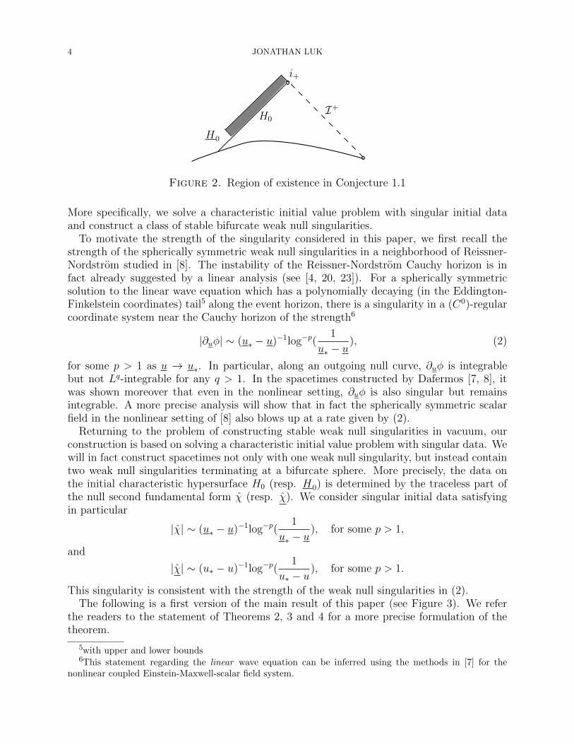
Figure 2. Region of existence in Conjecture 1.1
More specifically, we solve a characteristic initial value problem with singular initial dataand construct a class of stable bifurcate weak null singularities.
To motivate the strength of the singularity considered in this paper, we first recall thestrength of the spherically symmetric weak null singularities in a neighborhood of Reissner-Nordstrom studied in [8]. The instability of the Reissner-Nordstrom Cauchy horizon is infact already suggested by a linear analysis (see [4, 20, 23]). For a spherically symmetricsolution to the linear wave equation which has a polynomially decaying (in the Eddington-Finkelstein coordinates) tail5 along the event horizon, there is a singularity in a (C0)-regularcoordinate system near the Cauchy horizon of the strength6
|∂uφ| ∼ (u∗ − u)−1log−p(1
u∗ − u), (2)
for some p > 1 as u → u∗. In particular, along an outgoing null curve, ∂uφ is integrablebut not Lq-integrable for any q > 1. In the spacetimes constructed by Dafermos [7, 8], itwas shown moreover that even in the nonlinear setting, ∂uφ is also singular but remainsintegrable. A more precise analysis will show that in fact the spherically symmetric scalarfield in the nonlinear setting of [8] also blows up at a rate given by (2).
Returning to the problem of constructing stable weak null singularities in vacuum, ourconstruction is based on solving a characteristic initial value problem with singular data. Wewill in fact construct spacetimes not only with one weak null singularity, but instead containtwo weak null singularities terminating at a bifurcate sphere. More precisely, the data onthe initial characteristic hypersurface H0 (resp. H0) is determined by the traceless part ofthe null second fundamental form χ (resp. χ). We consider singular initial data satisfyingin particular
|χ| ∼ (u∗ − u)−1log−p(1
u∗ − u), for some p > 1,
and
|χ| ∼ (u∗ − u)−1log−p(1
u∗ − u), for some p > 1.
This singularity is consistent with the strength of the weak null singularities in (2).The following is a first version of the main result of this paper (see Figure 3). We refer
the readers to the statement of Theorems 2, 3 and 4 for a more precise formulation of thetheorem.
5with upper and lower bounds6This statement regarding the linear wave equation can be inferred using the methods in [7] for the
nonlinear coupled Einstein-Maxwell-scalar field system.
WEAK NULL SINGULARITIES IN GENERAL RELATIVITY 5
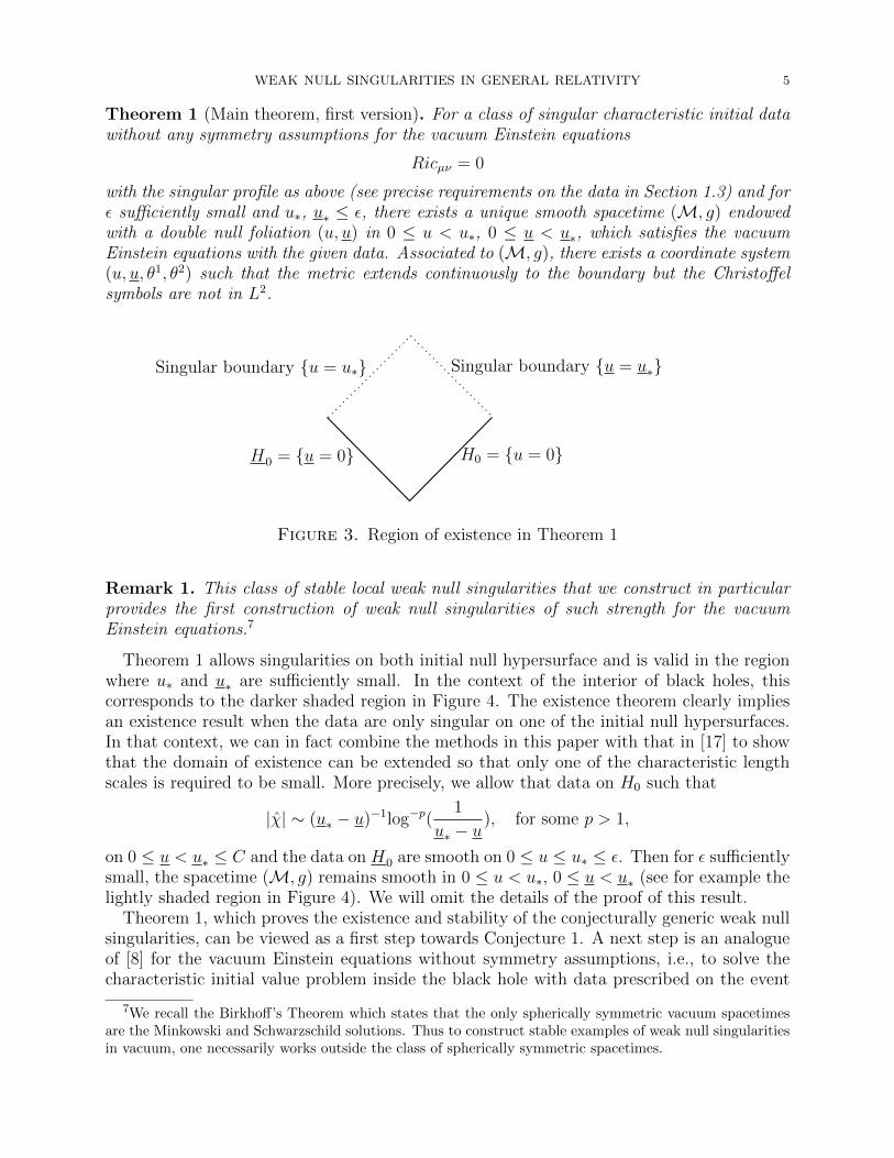
Theorem 1 (Main theorem, first version). For a class of singular characteristic initial datawithout any symmetry assumptions for the vacuum Einstein equations
Ricµν = 0
with the singular profile as above (see precise requirements on the data in Section 1.3) and forε sufficiently small and u∗, u∗ ≤ ε, there exists a unique smooth spacetime (M, g) endowedwith a double null foliation (u, u) in 0 ≤ u < u∗, 0 ≤ u < u∗, which satisfies the vacuumEinstein equations with the given data. Associated to (M, g), there exists a coordinate system(u, u, θ1, θ2) such that the metric extends continuously to the boundary but the Christoffelsymbols are not in L2.
H0 = u = 0H0 = u = 0
Singular boundary u = u∗ Singular boundary u = u∗
Figure 3. Region of existence in Theorem 1
Remark 1. This class of stable local weak null singularities that we construct in particularprovides the first construction of weak null singularities of such strength for the vacuumEinstein equations.7
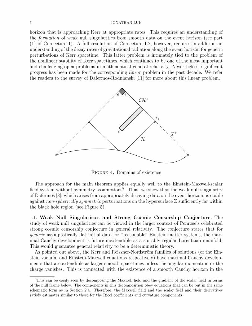
Theorem 1 allows singularities on both initial null hypersurface and is valid in the regionwhere u∗ and u∗ are sufficiently small. In the context of the interior of black holes, thiscorresponds to the darker shaded region in Figure 4. The existence theorem clearly impliesan existence result when the data are only singular on one of the initial null hypersurfaces.In that context, we can in fact combine the methods in this paper with that in [17] to showthat the domain of existence can be extended so that only one of the characteristic lengthscales is required to be small. More precisely, we allow that data on H0 such that
|χ| ∼ (u∗ − u)−1log−p(1
u∗ − u), for some p > 1,
on 0 ≤ u < u∗ ≤ C and the data on H0 are smooth on 0 ≤ u ≤ u∗ ≤ ε. Then for ε sufficientlysmall, the spacetime (M, g) remains smooth in 0 ≤ u < u∗, 0 ≤ u < u∗ (see for example thelightly shaded region in Figure 4). We will omit the details of the proof of this result.
Theorem 1, which proves the existence and stability of the conjecturally generic weak nullsingularities, can be viewed as a first step towards Conjecture 1. A next step is an analogueof [8] for the vacuum Einstein equations without symmetry assumptions, i.e., to solve thecharacteristic initial value problem inside the black hole with data prescribed on the event
7We recall the Birkhoff’s Theorem which states that the only spherically symmetric vacuum spacetimesare the Minkowski and Schwarzschild solutions. Thus to construct stable examples of weak null singularitiesin vacuum, one necessarily works outside the class of spherically symmetric spacetimes.
6 JONATHAN LUK
horizon that is approaching Kerr at appropriate rates. This requires an understanding ofthe formation of weak null singularities from smooth data on the event horizon (see part(1) of Conjecture 1). A full resolution of Conjecture 1.2, however, requires in addition anunderstanding of the decay rates of gravitational radiation along the event horizon for genericperturbations of Kerr spacetime. This latter problem is intimately tied to the problem ofthe nonlinear stability of Kerr spacetimes, which continues to be one of the most importantand challenging open problems in mathematical general relativity. Nevertheless, significantprogress has been made for the corresponding linear problem in the past decade. We referthe readers to the survey of Dafermos-Rodnianski [11] for more about this linear problem.
CH+
I+
H+
i+
ε
ε
ε
Figure 4. Domains of existence
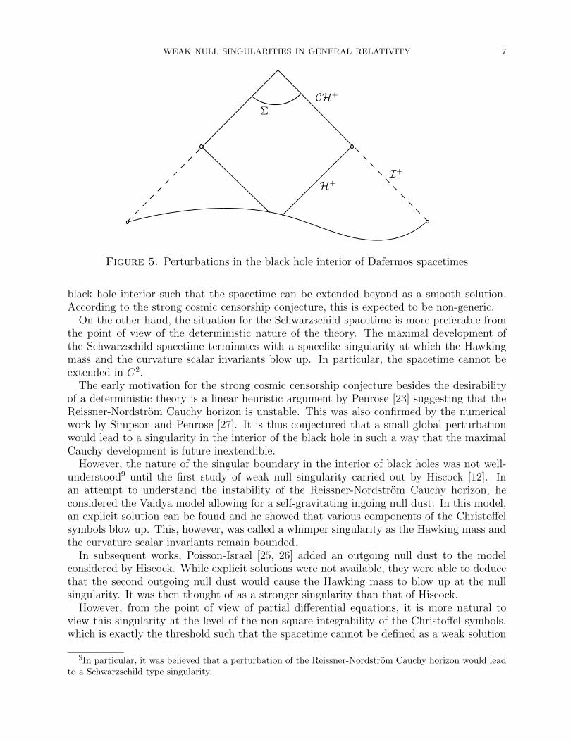
The approach for the main theorem applies equally well to the Einstein-Maxwell-scalarfield system without symmetry assumptions8. Thus, we show that the weak null singularityof Dafermos [8], which arises from appropriately decaying data on the event horizon, is stableagainst non-spherically symmetric perturbations on the hypersurface Σ sufficiently far withinthe black hole region (see Figure 5).
1.1. Weak Null Singularities and Strong Cosmic Censorship Conjecture. Thestudy of weak null singularities can be viewed in the larger context of Penrose’s celebratedstrong cosmic censorship conjecture in general relativity. The conjecture states that forgeneric asymptotically flat initial data for “reasonable” Einstein-matter systems, the max-imal Cauchy development is future inextendible as a suitably regular Lorentzian manifold.This would guarantee general relativity to be a deterministic theory.
As pointed out above, the Kerr and Reissner-Nordstrom families of solutions (of the Ein-stein vacuum and Einstein-Maxwell equations respectively) have maximal Cauchy develop-ments that are extendible as larger smooth spacetimes unless the angular momentum or thecharge vanishes. This is connected with the existence of a smooth Cauchy horizon in the
8This can be easily seen by decomposing the Maxwell field and the gradient of the scalar field in termsof the null frame below. The components in this decomposition obey equations that can be put in the sameschematic form as in Section 2.4. Therefore, the Maxwell field and the scalar field and their derivativessatisfy estimates similar to those for the Ricci coefficients and curvature components.
WEAK NULL SINGULARITIES IN GENERAL RELATIVITY 7
CH+
I+
H+
Σ
Figure 5. Perturbations in the black hole interior of Dafermos spacetimes
black hole interior such that the spacetime can be extended beyond as a smooth solution.According to the strong cosmic censorship conjecture, this is expected to be non-generic.
On the other hand, the situation for the Schwarzschild spacetime is more preferable fromthe point of view of the deterministic nature of the theory. The maximal development ofthe Schwarzschild spacetime terminates with a spacelike singularity at which the Hawkingmass and the curvature scalar invariants blow up. In particular, the spacetime cannot beextended in C2.
The early motivation for the strong cosmic censorship conjecture besides the desirabilityof a deterministic theory is a linear heuristic argument by Penrose [23] suggesting that theReissner-Nordstrom Cauchy horizon is unstable. This was also confirmed by the numericalwork by Simpson and Penrose [27]. It is thus conjectured that a small global perturbationwould lead to a singularity in the interior of the black hole in such a way that the maximalCauchy development is future inextendible.
However, the nature of the singular boundary in the interior of black holes was not well-understood9 until the first study of weak null singularity carried out by Hiscock [12]. Inan attempt to understand the instability of the Reissner-Nordstrom Cauchy horizon, heconsidered the Vaidya model allowing for a self-gravitating ingoing null dust. In this model,an explicit solution can be found and he showed that various components of the Christoffelsymbols blow up. This, however, was called a whimper singularity as the Hawking mass andthe curvature scalar invariants remain bounded.
In subsequent works, Poisson-Israel [25, 26] added an outgoing null dust to the modelconsidered by Hiscock. While explicit solutions were not available, they were able to deducethat the second outgoing null dust would cause the Hawking mass to blow up at the nullsingularity. It was then thought of as a stronger singularity than that of Hiscock.
However, from the point of view of partial differential equations, it is more natural toview this singularity at the level of the non-square-integrability of the Christoffel symbols,which is exactly the threshold such that the spacetime cannot be defined as a weak solution
9In particular, it was believed that a perturbation of the Reissner-Nordstrom Cauchy horizon would leadto a Schwarzschild type singularity.
8 JONATHAN LUK
to the Einstein equations. From this perspective, the singularity of Poisson-Israel is asstrong as that of Hiscock and both singularities can be viewed as terminal boundaries forthe spacetimes in question.
While the Christoffel symbols blow up at the Cauchy horizon, one can also think thatthe Cauchy horizon is “stable” in the sense that no singularity arises before the “originalCauchy horizon”. In particular, there is no spacelike portion of the singular boundary ina neighborhood of timelike infinity. This is thus contrary to the case of the Schwarzschildspacetime. This weak null singularity picture has been further explored and justified in manynumerical works (see [1, 2, 3]).
As we described before, the aforementioned picture of the interior of black holes was finallyestablished by Dafermos in the context of the spherically symmetric Einstein-Maxwell-scalarfield system [7]. This is the main motivation for our present work in which we initiatethe study of weak null singularities of similar strength in vacuum without any symmetryassumptions.
Finally, we note that a class of analytic spacetimes with slightly weaker singularitieshave been previously constructed in [22]. While this class of spacetime is more restrictive,as discussed in [22], it nonetheless admits the full “functional degrees of freedom” of theEinstein equations.
1.2. Comparison with Impulsive Gravitational Waves. As pointed out by Dafermos[9], the weak null singularities that we consider in this paper share many similarities withimpulsive gravitational waves. The latter are vacuum spacetimes admitting null hypersur-faces which support delta function singularities in the Riemann curvature tensor. Explicitexamples were first constructed by Penrose [24], Khan-Penrose [14] and Szekeres [28]. Inthese spacetimes, while the Christoffel symbols are not continuous, they remain bounded.Therefore, in contrast with the weak null singularities that we consider here, these impul-sive gravitational waves are not terminal singularities. In fact, the solution to the vacuumEinstein equation extends beyond the singularity and is smooth except across the singularhypersurface. Nevertheless, both scenarios represent singularities propagating along null hy-persurfaces and from a mathematical point of view, the proofs of the existence theory forthese singularities share many common features.
In recent joint works with Rodnianski [19, 18], we initiated the rigorous mathematicalstudy for general impulsive gravitational waves without symmetry assumptions. We con-structed the impulsive gravitational waves via solving the characteristic initial problem suchthat the initial data admit curvature delta singularities supported on an embedded 2-sphere.One of the new ideas in the proof is the use of renormalized energy estimates for the curva-ture components, i.e., instead of controlling the spacetime curvature components in L2, wesubtract off an L∞ correction from some curvature components. This allowed us to derivea closed system of L2 estimates which is completely independent of the singular curvaturecomponents.
In [18], when the interaction of impulsive gravitational waves was studied, we also extendedthe analysis to include a class of spacetimes such that when measured in the worst direction,the Christoffel symbols are merely in L2. We proved an existence and uniqueness theorem forspacetimes with such low regularity and showed that the spacetime solution can be extendedbeyond the singularities. Notice that this result is in fact sharp: This is because if theChristoffel symbols fail to be square-integrable, the spacetime cannot be extended as a weaksolution to the Einstein equations (see footnote 1).

WEAK NULL SINGULARITIES IN GENERAL RELATIVITY 9
By contrast, the spacetimes considered in this paper have Christoffel symbols which are10
not in L2. Even though the weak null singularities are terminal singularities in the sensethat there cannot be an existence theory beyond them, the theory developed in [19, 18] canbe extended to control the spacetime up to the singularity. Moreover, our main theorem,which allows for two weak null singularities terminating at their intersection, can be viewedas an extension of the result in [18] on the interaction of two impulsive gravitational waves.In particular, the renormalized energy of [19, 18] plays an important role in the proof ofour main theorem. However, even after renormalization, the renormalized curvature is stillsingular (i.e., not in L2) and has to be dealt with using an additional weighted estimate.
1.3. Description of the Main Results. Our setup is the characteristic initial value prob-lem with initial data given on two null hypersurfaces H0 and H0 intersecting at a 2-sphereS0,0 (see Figure 6). We will follow the general notations in [15, 5, 16].
H0H0
S0,0
e3 e4
Figure 6. The Basic Setup
We introduce a null frame e1, e2, e3, e4 adapted to a double null foliation (u, u) (seeSection 2.1). Denote the constant u hypersurfaces by Hu, the constant u hypersurfaces byHu and their intersections by Su,u = Hu ∩ Hu. Decompose the Riemann curvature tensorwith respect to the null frame e1, e2, e3, e4:
αAB = R(eA, e4, eB, e4), αAB = R(eA, e3, eB, e3),
βA =1
2R(eA, e4, e3, e4), β
A=
1
2R(eA, e3, e3, e4),
ρ =1
4R(e4, e3, e4, e3), σ =
1
4∗R(e4, e3, e4, e3).
We define also the Gauss curvature of the 2-spheres associated to the double null foliationto be K. Define also the following Ricci coefficients with respect to the null frame:
χAB = g(DAe4, eB), χAB
= g(DAe3, eB),
ηA = −1
2g(D3eA, e4), η
A= −1
2g(D4eA, e3),
ω = −1
4g(D4e3, e4), ω = −1
4g(D3e4, e3),
ζA =1
2g(DAe4, e3).
Let χ (resp. χ) be the traceless part of χ (resp. χ).
10In fact, we allow initial data to be in Lp only for p = 1, but not for any p > 1.
10 JONATHAN LUK
The data on H0 are given on 0 ≤ u < u∗ such that χ becomes singular as u → u∗.Similarly, the data on H0 is given on 0 ≤ u < u∗ such that χ becomes singular as u→ u∗.
More precisely, let f1 : [0, u∗)→ R be a smooth function such that f1(x) ≥ 0 is decreasingand ∫ u∗
0
1
f1(x)2dx <∞.
(resp. let f2 : [0, u∗)→ R be a smooth function such that f2(x) ≥ 0 is decreasing and∫ u∗
0
1
f2(x)2dx <∞.)
For example, f1 can be taken to be f1(x) = (u∗ − x)12 logp( 1
u∗−x) for p > 1
2.
Our main theorem shows local existence for a class of singular initial data with11
|χ(0, u)| . f1(u)−2, |χ(u, 0)| . f2(u)−2.
We construct a (unique) solution (M, g) to the vacuum Einstein equations in the regionu < u∗, u < u∗, where u∗, u∗ ≤ ε, and∫ u∗
0
f1(u)−2du,
∫ u∗
0
f2(u)−2du ≤ ε2. (3)
Here, (u, u) is a double null foliation for (M, g) and the metric g takes the form
g = −2Ω2(du⊗ du+ du⊗ du) + γAB(dθA − bAdu)⊗ (dθB − bBdu)
in the (u, u, θ1, θ2) coordinate system (to be defined in Section 2.2). Define also ∇ to be theinduced Levi-Cevita connection on the 2-spheres of constant u and u, i.e., Su,u, and ∇3, ∇4
to be the projections of the covariant derivatves D3, D4 to the tangent space of Su,u. Ourmain theorem (Theorem 1) can be stated precisely as a combination of Theorems 2, 3 and4. The first main result is the following theorem, which shows the existence of a spacetimeup to the (potentially singular) null boundaries:
Theorem 2. Consider the characteristic initial value problem for
Ricµν = 0 (4)
with data that are smooth on H0 ∩ 0 ≤ u < u∗ and H0 ∩ 0 ≤ u < u∗ such that
• There exists an atlas such that in each coordinate chart with local coordinates (θ1, θ2),the initial metric γ0 on S0,0 obeys
d ≤ det γ0 ≤ D,
and ∑i1+i2≤6
|( ∂
∂θ1)i1(
∂
∂θ2)i2γBC | ≤ D.
• The metric on H0 and H0 satisfies the gauge conditions
Ω = 1 on H0 and H0
andbA = 0 on H0.
11We assume also bounds for the angular derivatives which are consistent with this singular profile (seethe precise statement in Theorem 2).
WEAK NULL SINGULARITIES IN GENERAL RELATIVITY 11
• The Ricci coefficients on the initial hypersurface H0 verify∑i≤5
supu||f1
2(u)∇iχ||L2(S0,u) ≤ D,
∑i≤4
supu||∇iζ||L2(S0,u) ≤ D,
∑i≤4
supu||∇itrχ||L2(S0,u) ≤ D.
• The Ricci coefficients on the initial hypersurface H0 verify∑i≤5
supu||f2
2(u)∇iχ||L2(Su,0) ≤ D,
∑i≤4
supu||∇iζ||L2(Su,0) ≤ D,
∑i≤4
supu||∇itrχ||L2(Su,0) ≤ D.
Then for ε sufficiently small (depending only on d and D) and u∗, u∗ ≤ ε, ||f1(u)−1||L2u,
||f2(u)−1||L2u< ε, there exists a unique spacetime (M, g) endowed with a double null foliation
(u, u) in 0 ≤ u < u∗ and 0 ≤ u < u∗, which is a solution to the vacuum Einstein equations (4)with the given data. Moreover, the spacetime remains smooth in 0 ≤ u < u∗ and 0 ≤ u < u∗.
Remark 2. In the following, we will only prove a priori estimates for spacetimes arising fromthese initial data (see Theorem 5 below). The existence of a spacetime and the propagationof regularity follow from standard arguments. (For an example of this argument in lowregularity, see Sections 4 and 5 in [19]. See also Chapter 16 in [5].)
Remark 3. In order to simplify notations, we will omit the subscripts 1 and 2 in the weightfunctions f1 and f2. They can be inferred from whether f is a function of u or u.
Remark 4. In Section 4, we will construct a class of characteristic initial data which satisfiesthe assumptions of Theorem 2.
While the weight f in the spacetime norms allows the spacetime to be singular, the space-time metric can be extended beyond the singular hypersurfaces Hu∗ and Hu∗
continuously.
Theorem 3. Under the assumptions of Theorem 2, the spacetime (M, g) can be extendedcontinuously up to and beyond the singular boundaries Hu∗
:= u = u∗, Hu∗ := u = u∗.Moreover, the induced metric and null second fundamental form on the interior of the limitinghypersurfaces Hu∗
and Hu∗ are regular. More precisely, for any coordinate chart Ui on S0,0,the metric components γ, b, Ω satisfy the following estimates in the coordinate chart givenby Ui(u, u) := Φu Φu(Ui), where Φu and Φu are the diffeomorphisms generated by L and L
respectively12: ∑i1+i2≤4
sup0≤u≤u∗
‖( ∂
∂θ1)i1(
∂
∂θ2)i2(γ, b,Ω)‖L2(Ui(u,u∗))
≤ C.
12See definition of L and L in Section 2.1.
12 JONATHAN LUK
Moreover, for any fixed U < u∗, we have the following bounds for the Ricci coefficientsχ, trχ, ω, η, η: ∑
j≤1
∑i≤3−j
sup0≤u≤U
‖∇j3∇i(χ, trχ, ω, η, η)‖L2(Su,u∗ ) ≤ CU .
Similar regularity statements hold on Hu∗.
Remark 5. If we assume in addition that the higher angular derivatives of χ are bounded inL1uL∞(S), then the metric and the second fundamental form also inherit higher regularity in
the interior of Hu∗. In particular, if all angular derivatives of χ are bounded in L1
uL∞(S),
then the metric restricted to Hu∗∩ 0 ≤ u ≤ U is smooth along the directions tangential to
Hu∗. Similar statements hold on Hu∗. We will omit the details.
Moreover, we show that if initially the data are indeed singular, then Hu∗ and Hu∗are
terminal singularities of the spacetime in the following sense:
Theorem 4. If, in addition to the assumptions of Theorem 2, we also have the followingfor the initial data ∫ u∗
0
|χ(0, u)|2du =∞
along Lebesgue-almost every null generator on H0, then the Christoffel symbols in the coor-dinate system (u, u, θ1, θ2) do not belong to L2 in a neighborhood of any point on Hu∗
.Similarly if the initial data satisfy∫ u∗
0
|χ(u, 0)|2du =∞
along Lebesgue-almost every null generator on H0, then the Christoffel symbols in the coor-dinate system (u, u, θ1, θ2) do not belong to L2 in a neighborhood of any point on Hu∗.
Remark 6. Theorem 4 guarantees that if we extend the spacetime metric continuously in theobvious differentiable structure given by the coordinate system (u, u, θ1, θ2), then the Christof-fel symbols are non-square-integrable in the extension. However, it is an open problemwhether the spacetime admits any continuous extensions with square integrable Christoffelsymbols.
1.4. Main Ideas of the Proof. All the known proofs of regularity for the Einstein equationswithout symmetry assumptions rely on L2 estimates on the metric and its derivatives or theRiemann curvature tensor and its derivatives. Let us denote schematically by Γ a generalRicci coefficient and by Ψ a general curvature component decomposed with respect to a nullframe adapted to the double null foliation. In the double null foliation gauge (see for example,[15, 5]), the standard approach to obtain a priori bounds is to couple the L2 estimates forthe curvature components ∫
H
Ψ2 +
∫H
Ψ2 ≤ Data +
∫∫ΓΨΨ
with the estimates for the Ricci coefficients obtained using the transport equations
∇3Γ = Ψ + ΓΓ,
∇4Γ = Ψ + ΓΓ.
WEAK NULL SINGULARITIES IN GENERAL RELATIVITY 13
However, in the setting of two weak null singularities, none of the spacetime curvaturecomponents α, β, ρ, σ, β, α are in L2!
Nevertheless, while these curvature components are singular, the nature of their singularityis specific. More precisely, while the spacetime curvature components ρ and σ are not in L2,they can be written as a sum of some regular intrinsic curvature components K and σ (seefurther discussion in Section 1.4.1) which belong to L2 and terms which are quadratic in Γ.We therefore prove L2 estimates for K and σ, which we will call the “renormalized curvaturecomponents” (see [19, 18]). Moreover, by considering (K, σ) instead of (ρ, σ), we removeall appearances of α and α in the estimates and so that we do not have to deal with thesingularities of α and α! It still remains to control the singular curvature components β andβ. Here, we make use of the fact that β and β are singular in a specific manner towards the
singular boundary Hu∗and Hu∗ respectively. We therefore introduce degenerate L2 norms
that incorporate these singularities. We will explain the renormalization and the degenerateestimates in more detail below.
1.4.1. Renormalized Energy Estimates. As described above, a main ingredient of the proofof the main theorem is the renormalized energy estimates introduced in [19, 18] in the studyof impulsive gravitational waves. This can be seen as follows. For the class of weak nullsingularities that we consider, while the L/ L derivative of the spacetime metric blows up, themetric restricted to the 2-sphere remains regular in the angular directions. Since the Gausscurvature K is intrinsic to the 2-spheres, it remains bounded. On the other hand, by theGauss equation:
K = −ρ+1
2χ · χ− 1
4trχtrχ
and the fact that trχ and χ blow up at u = u∗, ρ also blows up at u = u∗. In view of this,we estimate the Gauss curvature K instead of the spacetime curvature component ρ.
Indeed, we see that the Gauss curvature K satisfies equations such that the right handside contains terms that are less singular than the terms in the corresponding equation forρ. More precisely, for the curvature component ρ, we have (up to lower order terms) theBianchi equation
∇4ρ+3
2trχρ = div β − 1
2χ · α + ...,
which contains the non-integrable curvature component α. On the other hand, the Gausscurvature obeys the equation (see (12))
∇4K + trχK = −div β + ...,
where there are no terms containing α or are quadratic in trχ, χ and ω, i.e. every term onthe right hand side of the equation is integrable in the u direction13.
In a similar fashion, by considering the renormalized curvature component14
σ := σ +1
2χ ∧ χ
13The can be compared with the renormalization introduced in [19] and [18], where we estimated ρ =ρ − 1
2 χ · χ instead of ρ. Whereas the renormalization using ρ allows one to eliminate α in the estimates,
it nonetheless introduces a term 14 trχ|χ|2, which is not integrable in the u direction in the setting of the
present paper. Instead, by studying the equation for K, we see none of these terms which are quadratic intrχ, χ or ω! This fact can also be derived directly by considering the equations for ∇4K using the intrinsicdefinition of the Gauss curvature.
14This is in fact related to the intrinsic curvature of the normal bundle to Su,u.
14 JONATHAN LUK
instead of σ, we see that it satisfies an equation such that all the terms on the right handside are integrable in the u direction.
One consequence of the renormalization is that we have completely removed the appear-ances of the curvature component α in the equations. In fact, as in [19, 18], this allows usto derive a set of estimates for the renormalized curvature component without requiring anyinformation on the curvature component α.
Moreover, when considering the equations for ∇3K and ∇3σ for the renormalized cur-vature components, one sees that α does not appear and all the terms are integrable inthe u direction. Therefore, although α or α can be very singular near one of the singularboundaries, we do not need to derive any estimates for them!
1.4.2. Degenerate L2 Estimates. Since the renormalization above deals with the singularityin the ρ and σ components and avoids any information on α and α, it remains to deriveappropriate L2 estimates for β and β.
The main observation is that while β and β are both singular and fail to be in L2, theirsingularities can be captured quantitatively. Consider the curvature component β. Since theblow up rate of trχ and χ can be bounded above by f(u)−2, in view of the Codazzi equationsin (10), β is also bounded above by f(u)−2. In particular, while β is only in L1
u but not in
Lpu for any p > 1, the assumptions on the initial data allow us to control f(u)β in L2u. We
will thus incorporate this blow up in the norms and will be able to still use an L2 basedestimate.
The energy estimates will be obtained directly from two sets of Bianchi equations instead ofusing the Bel-Robinson tensor. Notice that since the energy estimates for K, σ are obtainedeither together with that for β or that for β, even though K and σ are regular, their energyestimates degenerate. Therefore, at the highest level of derivatives, we have to contend withthe weaker L2 estimates for these curvature components.
A potentially more serious challenge is that the introduction of the degenerate weightsin u and u would create terms that cannot be estimated by the energy estimates them-selves. Nevertheless, since the weights are chosen to be decreasing towards the future, theseuncontrollable terms in fact possess a good sign.
1.4.3. Estimates for the Ricci Coefficients. As indicated above, the Ricci coefficients enteras error terms in the energy estimates. Thus, to close all the estimates, we need to controlthe Ricci coefficients Γ by using the transport equations which in turn have the curvaturecomponents in the source terms. Since the various Ricci coefficients have different singularbehavior, we separate them according to the bounds that they obey. More precisely, denoteby ψH the components that behave like f(u)−2 as u → u∗; by ψH the components thatbehave like f(u)−2 as u→ u∗; and by ψ the components that are bounded.
For the singular Ricci coefficients ψH , we have the following schematic transport equations:
∇3ψH = K +∇ψ + ψψ + ψHψH .
The first three terms on the right hand side of this equation are bounded while the last termis singular. Nevertheless, the singularity of ψH still allows it to be controlled in L1 alongthe e3 direction. Thus, this equation can be integrated to show that the initial (singular)bounds for ψH can be propagated. It is important that the terms of the form ψHψH andψHψH do not appear in the equations. A similar structure can also be seen in the equation

WEAK NULL SINGULARITIES IN GENERAL RELATIVITY 15
for the other singular Ricci coefficients ψH , which takes the form
∇4ψH = K +∇ψ + ψψ + ψHψH .
For the regular Ricci coefficients ψ, we have transport equations of the form
∇4ψ = β + ψψH , or ∇3ψ = β + ψψH .
The bounds that we prove show that the right hand side is integrable and therefore ψ remainsbounded. For example, in the ∇4 equation, it is important that we do not have terms ofthe form ψHψH , ψψH , ψHψH and ψHψH , which are not uniformly bounded after integratingalong the e4 direction.
1.4.4. Null Structure in the Energy Estimates. A priori, the degenerate L2 estimates that weintroduce may not be sufficient to control the error terms. Nevertheless, the vacuum Einsteinequations possess a remarkable null structure which allows one to close the estimates usingonly the degenerate L2 estimates.
For example, in the energy estimates for the singular component β, we have
||f(u)β||2L2(H) ≤ Data + ||f 2(u)(βψHβ + βψHβ + βψK)||L1uL
1uL
1(S).
To estimate the first term, it suffices to note that ψH , while singular, can be shown to besmall after integrating along the u direction. Thus the first term can be controlled usingGronwall’s inequality. For the second term, since the singularity for β has the same strengthas that for ψH (and similarly the singularity for β has the same strength as that for ψH),the singularity in this term is similar to that in the first term and can also be bounded. Thefinal term is less singular since ψ and K are both uniformly bounded.15 Notice that if othercombinations of curvature terms and Ricci coefficients such as βψHβ, βψHβ or βψHK appearin the error terms, the degenerate energy will not be strong enough to close the bounds!
In order to close all the estimates, we need to commute also with higher derivatives. As in[19, 18], we will only commute with angular covariant derivatives. These commutations willnot introduce terms that are more singular. Moreover, the null structure of the estimatesindicated above is also preserved under these commutations.
Similar to [19, 18], the renormalization introduces error terms in the energy estimates suchthat the Ricci coefficients have one more derivative compared to the curvature components.These terms cannot be estimated via transport equations alone but are controlled using alsoelliptic estimates on the spheres. A form of null structure similar to that described abovealso makes an appearance in these elliptic estimates, allowing all the bounds to be closed.
1.5. Outline of the Paper. We end the introduction with an outline of the remainder ofthe paper. In Section 2, we introduce the basic setup of the paper, including the double nullfoliation, the coordinate system and the Einstein vacuum equations recast in terms of thegeometric quantities associated to the double null foliation. In Section 3, we introduce thenorms used in the paper and state a theorem on a priori estimates (Theorem 5) which implyour main existence theorem (Theorem 2). In Section 4, we construct a class of characteristicinitial data satisfying the assumptions of Theorem 2. In Sections 5-8, we prove Theorem5. In Section 5, we obtain the estimates for the metric components and derive functionalinequalities useful in our setting. Then in Sections 6 and 7, we prove bounds for the Riccicoefficients assuming control of the curvature components. In Section 8, we close all the
15Although as pointed out before, the highest derivative estimates for K in the energy norm suffer a lossas one approaches the singular boundaries, this term can nevertheless be controlled.
16 JONATHAN LUK
estimates by obtaining bounds for the curvature components. Finally, in Section 9, wediscuss the nature of the singular boundary and prove Theorems 3 and 4.
2. Basic Setup
2.1. Double Null Foliation. For a smooth16 spacetime in a neighborhood of S0,0, we definea double null foliation as follows: Let u and u be solutions to the eikonal equation
gµν∂µu∂νu = 0, gµν∂µu∂νu = 0,
such that u = 0 on H0 and u = 0 on H0. Let
L′µ = −2gµν∂νu, L′µ = −2gµν∂νu.
These are null and geodesic vector fields. Let
2Ω−2 = −g(L′, L′).
Define
e3 = ΩL′, e4 = ΩL′
to be the normalized null pair such that
g(e3, e4) = −2
and
L = Ω2L′, L = Ω2L′
to be the so-called equivariant vector fields.In this paper, we will consider spacetime solutions to the vacuum Einstein equations (1)
in the gauge such that
Ω = 1, on H0 and H0.
The level sets of u (resp. u) are denoted by Hu (resp. Hu). The eikonal equations implythat Hu and Hu are null hypersurface. The intersections of the hypersurfaces Hu and Hu
are topologically 2-spheres, which we denote by Su,u. Note that the integral flows of L andL respect the foliation Su,u.
2.2. The Coordinate System. We define a coordinate system (u, u, θ1, θ2) in a neighbor-hood of S0,0 as follows: On the sphere S0,0, we have an atlas such that in the local coordinatesystem (θ1, θ2) in each coordinate chart, the metric γ is smooth, bounded and positive defi-nite. Recall that in a neighborhood of S0,0, u and u are solutions to the eikonal equations:
gµν∂µu∂νu = 0, gµν∂µu∂νu = 0.
We then require the coordinates to satisfy
L/ LθA = 0
on the initial hypersurface H0 and
L/ LθA = 0
16The spacetimes considered in this paper are not smooth at u = u∗ or u = u∗. However, since we firstconstruct the spacetime in the region u < u∗ ∩ u < u∗ in which the spacetime is smooth (see Theorem2), it suffices to define the double null foliation for smooth spacetimes.
WEAK NULL SINGULARITIES IN GENERAL RELATIVITY 17
in the spacetime region. Here, L/ L and L/ L denote the restriction of the Lie derivative toTSu,u (See [5], Chapter 1) and L and L are defined as in the Section 2.1. Relative to thecoordinate system (u, u, θ1, θ2), the null pair e3 and e4 can be expressed as
e3 = Ω−1
(∂
∂u+ bA
∂
∂θA
), e4 = Ω−1 ∂
∂u,
for some bA such that bA = 0 on H0, while the metric g takes the form
g = −2Ω2(du⊗ du+ du⊗ du) + γAB(dθA − bAdu)⊗ (dθB − bBdu).
2.3. Equations. We will recast the Einstein equations as a system for Ricci coefficients andcurvature components associated to a null frame e3, e4 defined above and an orthonormalframe17 eAA=1,2 tangent to the 2-spheres Su,u. We define the Ricci coefficients relative tothe null fame:
χAB = g(DAe4, eB), χAB
= g(DAe3, eB),
ηA = −1
2g(D3eA, e4), η
A= −1
2g(D4eA, e3),
ω = −1
4g(D4e3, e4), ω = −1
4g(D3e4, e3),
ζA =1
2g(DAe4, e3),
(5)
where DA = De(A). We also introduce the null curvature components,
αAB = R(eA, e4, eB, e4), αAB = R(eA, e3, eB, e3),
βA =1
2R(eA, e4, e3, e4), β
A=
1
2R(eA, e3, e3, e4),
ρ =1
4R(e4, e3, e4, e3), σ =
1
4∗R(e4, e3, e4, e3).
(6)
Here ∗R denotes the Hodge dual of R. We denote by ∇ the induced covariant derivativeoperator on Su,u and by ∇3, ∇4 the projections to Su,u of the covariant derivatives D3, D4
(see precise definitions in Chapter 3.1 of [15]).Observe that,
ω = −1
2∇4(log Ω), ω = −1
2∇3(log Ω),
ηA = ζA +∇A(log Ω), ηA
= −ζA +∇A(log Ω).(7)
Define the following contractions of the tensor product φ(1) and φ(2) with respect to themetric γ:
φ(1) · φ(2) := (γ−1)AC(γ−1)BDφ(1)ABφ
(2)CD for symmetric 2-tensors φ
(1)AB, φ
(2)AB,
φ(1) · φ(2) := (γ−1)ABφ(1)A φ
(2)B for 1-forms φ
(1)A , φ
(2)A ,
(φ(1) · φ(2))A := (γ−1)BCφ(1)ABφ
(2)C for a symmetric 2-tensor φ
(1)AB and a 1-form φ
(2)A ,
(φ(1)⊗φ(2))AB := φ(1)A φ
(2)B + φ
(1)B φ
(2)A − γAB(φ(1) · φ(2)) for one forms φ
(1)A , φ
(2)A ,
φ(1) ∧ φ(2) := ε/ AB(γ−1)CDφ(1)ACφ
(2)BD for symmetric two tensors φ
(1)AB, φ
(2)AB,
17Of course the orthonormal frame is only defined locally. Alternatively, the capital Latin indices can beunderstood as abstract indices.
18 JONATHAN LUK
where ε/ is the volume form associated to the metric γ. We also define by ∗ for 1-forms andsymmetric 2-tensors respectively as follows (note that on 1-forms this is the Hodge dual onSu,u):
∗φA :=γACε/CBφB,
∗φAB :=γBDε/DCφAC .
Define the operator ∇⊗ on a 1-form φA by
(∇⊗φ)AB := ∇AφB +∇BφA − γABdiv φ.
For totally symmetric tensors, define the div and curl operators as follows
(div φ)A1...Ar := ∇BφBA1...Ar ,
(curl φ)A1...Ar := ε/ BC∇BφCA1...Ar .
Define also the trace of totally symmetric tensors to be
(trφ)A1...Ar−1 := (γ−1)BCφBCA1...Ar−1 .
We separate the trace and traceless part of χ and χ. Let χ and χ be the traceless partsof χ and χ respectively. Then χ and χ satisfy the following null structure equations:
∇4trχ+1
2(trχ)2 = −|χ|2 − 2ωtrχ,
∇4χ+ trχχ = −2ωχ− α,
∇3trχ+1
2(trχ)2 = −2ωtrχ− |χ|2,
∇3χ+ trχ χ = −2ωχ− α,
∇4trχ+1
2trχtrχ = 2ωtrχ+ 2ρ− χ · χ+ 2div η + 2|η|2,
∇4χ+1
2trχχ = ∇⊗η + 2ωχ− 1
2trχχ+ η⊗η,
∇3trχ+1
2trχtrχ = 2ωtrχ+ 2ρ− χ · χ+ 2div η + 2|η|2,
∇3χ+1
2trχχ = ∇⊗η + 2ωχ− 1
2trχχ+ η⊗η.
(8)
The other Ricci coefficients satisfy the following null structure equations:
∇4η = −χ · (η − η)− β,∇3η = −χ · (η − η) + β,
∇4ω = 2ωω − η · η +1
2|η|2 +
1
2ρ,
∇3ω = 2ωω − η · η +1
2|η|2 +
1
2ρ.
(9)
WEAK NULL SINGULARITIES IN GENERAL RELATIVITY 19
The Ricci coefficients also satisfy the following constraint equations
div χ =1
2∇trχ− 1
2(η − η) · (χ− 1
2trχ)− β,
div χ =1
2∇trχ+
1
2(η − η) · (χ− 1
2trχ) + β,
curl η = −curl η = σ +1
2χ ∧ χ,
K = −ρ+1
2χ · χ− 1
4trχtrχ,
(10)
with K the Gauss curvature of the spheres Su,u. The null curvature components satisfy thefollowing null Bianchi equations:
∇3α +1
2trχα = ∇⊗β + 4ωα− 3(χρ+∗ χσ) + (ζ + 4η)⊗β,
∇4β + 2trχβ = div α− 2ωβ + (2ζ + η) · α,∇3β + trχβ = ∇ρ+ 2ωβ +∗ ∇σ + 2χ · β + 3(ηρ+∗ ησ),
∇4σ +3
2trχσ = −div ∗β +
1
2χ ∧ α− ζ ∧ β − 2η ∧ β,
∇3σ +3
2trχσ = −div ∗β − 1
2χ ∧ α + ζ ∧ β − 2η ∧ β,
∇4ρ+3
2trχρ = div β − 1
2χ · α + ζ · β + 2η · β,
∇3ρ+3
2trχρ = −div β − 1
2χ · α + ζ · β − 2η · β,
∇4β + trχβ = −∇ρ+∗ ∇σ + 2ωβ + 2χ · β − 3(ηρ−∗ ησ),
∇3β + 2trχβ = −div α− 2ωβ − (−2ζ + η) · α,
∇4α +1
2trχα = −∇⊗β + 4ωα− 3(χρ−∗ χσ) + (ζ − 4η)⊗β.
(11)
where ∗ denotes the Hodge dual on Su,u.We now rewrite the Bianchi equations in terms of the Gauss curvature K of the spheres
Su,u and the renormalized curvature component σ defined by
σ = σ +1
2χ ∧ χ.
20 JONATHAN LUK
The Bianchi equations take the following form
∇3β + trχβ =−∇K +∗ ∇σ + 2ωβ + 2χ · β − 3(ηK −∗ ησ) +1
2(∇(χ · χ) +∗ ∇(χ ∧ χ))
+3
2(ηχ · χ+∗ ηχ ∧ χ)− 1
4(∇trχtrχ+ trχ∇trχ)− 3
4ηtrχtrχ,
∇4σ +3
2trχσ =− div ∗β − ζ ∧ β − 2η ∧ β − 1
2χ ∧ (∇⊗η)− 1
2χ ∧ (η⊗η),
∇4K + trχK =− div β − ζ · β − 2η · β +1
2χ · ∇⊗η +
1
2χ · (η⊗η)− 1
2trχdiv η − 1
2trχ|η|2,
∇3σ +3
2trχσ =− div ∗β + ζ ∧ β − 2η ∧ β +
1
2χ ∧ (∇⊗η) +
1
2χ ∧ (η⊗η),
∇3K + trχK =div β − ζ · β + 2η · β +1
2χ · ∇⊗η +
1
2χ · (η⊗η)− 1
2trχdiv η − 1
2trχ|η|2,
∇4β + trχβ =∇K +∗ ∇σ + 2ωβ + 2χ · β + 3(ηK +∗ ησ)− 1
2(∇(χ · χ)−∗ ∇(χ ∧ χ))
+1
4(∇trχtrχ+ trχ∇trχ)− 3
2(ηχ · χ−∗ ηχ ∧ χ) +
3
4ηtrχtrχ.
(12)
Notice that we have obtained a system for the renormalized curvature components in whichthe curvature components α and α do not appear.18
From now on, we will use capital Latin letters A ∈ 1, 2 for indices on the spheres Su,uand Greek letters µ ∈ 1, 2, 3, 4 for indices in the whole spacetime.
2.4. Schematic Notation. We define a schematic notation for the Ricci coefficients ac-cording to the estimates that they obey. Introduce the following conventions:19
ψ ∈ η, η, ψH ∈ trχ, χ, ω, ψH ∈ trχ, χ, ω.We will use this schematic notation only in the situations where the exact constant in
front of the term is irrelevant to the argument. We will denote by ψψ (or ψψH , etc) anarbitrary contraction with respect to the metric γ and by ∇ψ an arbitrary angular covariantderivative. ∇iψj will be used to denote the sum of all terms which are products of j factors,such that each factor takes the form ∇ikψ and that the sum of all ik’s is i, i.e.,
∇iψj =∑
i1+i2+...+ij=i
∇i1ψ∇i2ψ...∇ijψ︸ ︷︷ ︸j factors
.
We will use brackets to denote terms with one of the components in the brackets. Forinstance, the notation ψ(ψ, ψH) denotes the sum of all terms of the form ψψ or ψψH .
In this schematic notation, the Ricci coefficients ψH satisfy
∇3ψH = K +∇ψ + ψψ + ψHψH .
The Ricci coefficients ψH similarly obey
∇4ψH = K +∇ψ + ψψ + ψHψH .
18Moreover, compared to the renormalization in [19], this system do not contain the terms trχ|χ|2 and
trχ|χ|2 which would be uncontrollable in the context of this paper.19Notice that this definition is different form that in [19] since in the context of the present paper, trχ
and trχ verify different bounds compared to [19].
WEAK NULL SINGULARITIES IN GENERAL RELATIVITY 21
The Ricci coefficients ψ obey either one of the following equations:
∇3ψ = β + ψψH
or
∇4ψ = β + ψψH .
We also rewrite the Bianchi equations in the schematic notation:
∇3β+∇K −∗ ∇σ =∑
i1+i2=1
ψHψi1∇i2ψH + ψK +
∑i1+i2=1
ψi1ψ∇i2ψ
∇4σ + div ∗β =ψH σ + ψ∑
i1+i2+i3=1
ψi1∇i2ψ∇i3ψH ,
∇4K+div β =ψHK + ψ∑
i1+i2+i3=1
ψi1∇i2ψ∇i3ψH ,
∇3σ + div ∗β =ψH σ + ψ∑
i1+i2+i3=1
ψi1∇i2ψ∇i3ψH ,
∇3K−div β =ψHK + ψ∑
i1+i2+i3=1
ψi1∇i2ψ∇i3ψH ,
∇4β−∇K −∗ ∇σ =∑
i1+i2=1
ψHψi1∇i2ψH + ψK +
∑i1+i2=1
ψi1ψ∇i2ψ.
(13)
3. Norms
In this section, we define the norms that we will use to control the geometric quantities.We will in particular use the schematic notation defined in Section 2.4. Our norms will beof the form LpuL
quL
r(S), where Lpu and Lqu are defined with respect to the measures du anddu respectively and Lr(S) is defined for any tensors φ on Su,u by
‖φ‖Lr(Su,u) :=
(∫Su,u
(φA1A2...AnφA1A2...An)
r2
) 1r
,
where the integral is with respect to the volume form induced by γ.We define the following norms for the Ricci coefficients ψ for p ∈ [1,∞], i ∈ N:
Oi,p[ψ] := ||∇iψ||L∞u L∞u Lp(S). (14)
Define the following norms for the Ricci coefficients ψH for p ∈ [1,∞], i ∈ N:
Oi,p[ψH ] := ||f(u)∇iψH ||L2uL∞u L
p(S). (15)
Similarly, we define the following norms for the Ricci coefficients ψH for p ∈ [1,∞], i ∈ N:
Oi,p[ψH ] := ||f(u)∇iψH ||L2uL∞u L
p(S). (16)
As a shorthand, we define the following norm combining all of the norms above:
Oi,p :=∑
ψ∈η,η
Oi,p[ψ] +∑
ψH∈trχ,χ,ω
Oi,p[ψH ] +∑
ψH∈trχ,χ,ω
Oi,p[ψH ].
We make two remarks concerning these norms:
22 JONATHAN LUK
Remark 7. While the norms for ψH and ψH are based on L2 in u and u respectively, byvirtue of the weights f(u) and f(u), they actually control the L1 norms. More precisely,since
∫ u∗0
1f2(u′)
du′ < ε2 and∫ u∗
01
f2(u′)du′ < ε2, by the Cauchy-Schwarz inequality, we have
||∇iψH ||L1uL∞u L
p(S) ≤ CεOi,p[ψH ],
and
||∇iψH ||L1uL∞u L
p(S) ≤ CεOi,p[ψH ].
Remark 8. The norm Oi,p[ψH ] (resp. Oi,p[ψH ]) allows us to first take L∞ along the udirection (resp. u direction) before the L2 norm in u (resp. u) is taken. This is strongerthan the norms such that the order is reversed, i.e., we have
||f(u)∇iψH ||L∞u L2uL
p(S) ≤ COi,p[ψH ],
and
||f(u)∇iψH ||L∞u L2uL
p(S) ≤ COi,p[ψH ].
In addition to the above norms, we need to define norms for the highest derivatives forthe Ricci coefficients. Let
O4,2 :=||f(u)2∇4trχ||L∞u L∞u L2(S) + ||f(u)2∇4trχ||L∞u L∞u L2(S)
+ ||f(u)∇4(χ, ω)||L∞u L2uL
2(S) + ||f(u)∇4(η, η)||L∞u L2uL
2(S)
+ ||f(u)∇4(χ, ω)||L∞u L2uL
2(S) + ||f(u)∇4(η, η)||L∞u L2uL
2(S).
(17)
Remark 9. Here, note that for the norms for χ, ω, η, η, χ and ω, L∞ in u (or u) is taken
after L2 in u (or u). According to Remark 8, this is weaker than the Oi,2 norms definedabove.
Remark 10. Notice that the norms for the fourth derivatives of η and η come with a weightf(u) or f(u). This is in contrast to the lower order derivatives for η and η, which canbe estimated in L∞u L
∞u without any degeneration. The degeneration here arises from the
fact that these higher order derivatives are recovered from the energy estimates for ∇3K.These energy estimates for ∇3K, which are derived simultaneously with the estimates forthe singular components ∇3β or ∇3β, have a degeneration either in u or u.
We also define the curvature norms for the curvature components. For i ∈ N, let
Ri :=||f(u)∇iβ||L∞u L2uL
2(S) + ||f(u)∇i(K, σ)||L∞u L2uL
2(S)
+ ||f(u)∇i(K, σ)||L∞u L2uL
2(S) + ||f(u)∇iβ||L∞u L2uL
2(S).(18)
As a shorthand, we also let
R :=∑i≤3
Ri.
WEAK NULL SINGULARITIES IN GENERAL RELATIVITY 23
Finally, let Oini and Rini denote the corresponding norms for the initial data, i.e.
Oini :=∑i≤3
(||∇iψ||L∞u L2(S0,u) + ||∇iψ||L∞u L2(Su,0)
+ ||f(u)∇iψH ||L2uL
2(S0,u) + ||f(u)∇iψH ||L2uL
2(Su,0)
)+ ||f(u)2∇4trχ||L∞u L2(S0,u) + ||f(u)2∇4trχ||L∞u L2(Su,0)
+ ||∇4trχ||L∞u L2(S0,u) + ||∇4trχ||L∞u L2(Su,0)
+ ||f(u)∇4(χ, ω)||L2uL
2(S0,u) + ||∇4(η, η)||L2uL
2(S0,u)
+ ||f(u)∇4(χ, ω)||L2uL
2(Su,0) + ||∇4(η, η)||L2uL
2(Su,0)
and
Rini :=∑i≤3
(||f(u)∇iβ||L2
uL2(S0,u) + ||∇i(K, σ)||L2
uL2(S0,u)
+||∇i(K, σ)||L2uL
2(Su,0) + ||f(u)∇iβ||L2uL
2(Su,0)
).
In order to prove Theorem 2, we will establish a priori estimates for the geometric quan-tities in the above norms:
Theorem 5. Assume that the initial data for the characteristic initial value problem satisfythe assumptions of Theorem 2 with ε sufficiently small. Then there exists B depending onlyon D and d such that ∑
i≤3
Oi,2 + O4,2 +R ≤ B.
In the remainder of the paper, we will focus on the proof of Theorem 5 (after constructinginitial data sets in the next section). Standard methods show that Theorem 5 impliesTheorem 2. We will omit the details and refer the readers to [5, 19] for a proof that the apriori estimates imply the existence theorem.
Remark 11. The assumptions of Theorem 2 imply the boundedness of the following weightedL2 norms of the curvature components:∑
i≤3
||f(u)∇iβ||L2uL
2(S0,u) +∑i≤3
||∇i(K, σ)||L2uL
2(S0,u) ≤ D,
and ∑i≤3
||f(u)∇iβ||L2uL
2(Su,0) +∑i≤3
||∇i(K, σ)||L2uL
2(Su,0) ≤ D,
for some D depending only on D and d. These estimates for β, σ and β follow immediatelyfrom the constraint equations on the 2-spheres (see (10)). The bound for K follows afterintegrating the null Bianchi equations for K on each of the initial null hypersurfaces (see(12)).20 In particular, the assumptions of Theorem 2 imply that
Oini +Rini ≤ D.
20Notice that it is precisely for the initial bound for K that we require an extra derivative for χ on H0
(and χ on H0) in the assumptions of the theorem. This is related to the intrinsic loss of derivatives for the
characteristic initial value problem for second order hyperbolic systems (see [21]).
24 JONATHAN LUK
4. Construction of Initial Data Set
In this section, we construct initial data sets satisfying the assumptions of Theorems 2 and4. In particular, we show that the constraint equations can be solved for |χ(0, u)| ∼ (f(u))−2
and |χ(u, 0)| ∼ (f(u))−2. Our approach in this section follows closely that of Christodoulouin Chapter 2 of [5].
Assume for simplicity that S0,0 is a standard sphere of radius 1. Introduce21 the standard
stereographic coordinates (θ1, θ2) such that the standard metricγ on the sphere takes the
formγAB=
δAB(1 + 1
4|θ|2)2
.
Clearly, it suffices to construct initial data on H0 (with 0 ≤ u < u∗ for u∗ ≤ ε). Theconstruction on H0 is similar. On H0, we set Ω = 1 and therefore e4 = ∂
∂u. We will construct
a metric on H0 in the (u, θ1, θ2) coordinates taking the form
γAB = Φ2γAB, where γAB =mAB
(1 + 14|θ|2)2
(19)
and detmAB = 1 and Φ S0,0= 1. In order to ensure that m satisfies detm = 1, we write
m = exp Ψ,
with Ψ ∈ S, where S denotes the set of all matrices taking the form(a bb −a
).
We will impose upper and lower bounds on Ψ. Since there are no smooth globally non-vanishing Ψ ∈ S on the 2-sphere, we use the convention that . denotes that the quantity isbounded above by a uniform constant, while ∼ denotes that the quantity is bounded aboveby a uniform constant, and is bounded below at every (θ1, θ2) by a constant depending on(θ1, θ2) (where the constant is moreover allowed to vanish at finitely many isolated points).
We require Ψ ∈ S to satisfy22∑|J |≤N
|( ∂∂θ
)JΨ| . 1,
∑|J |≤N
|( ∂∂θ
)J ∂∂u
Ψ| . f(u)−2, | ∂∂u
Ψ| ∼ f(u)−2 (20)
for some sufficiently large integer N . Following [5], we have
χAB =1
2Φ2 ∂
∂uγAB, trχ =
2
Φ
∂Φ
∂u. (21)
We can also derive that
|χ|2γ =1
4(γ−1)AC(γ−1)BD
∂
∂uγAB
∂
∂uγCD.
Thus by (20), we have
|χ|2γ ∼ f(u)−4. (22)
21While we only write down one coordinate chart, it is implicit that we have two stereographic charts - thenorth pole chart and the south pole chart. In the following, when we derive the estimates for the geometricquantities, we only prove the bounds in a sufficiently large ball Bρ in each of these charts.
22Here and in the rest of this section, we use the notation that J = (j1, j2) ∈ (N ∪ 0) × (N ∪ 0) is amulti-index and ( ∂∂θ )J = ( ∂
∂θ1 )j1( ∂∂θ2 )j2 . We moreover denote |J | = j1 + j2.

WEAK NULL SINGULARITIES IN GENERAL RELATIVITY 25
In particular, this implies that the requirement in Theorem 4 is satisfied if∫ u∗
0f(u)−4du =∞.
By the equation
L/ ∂∂u
trχ = −1
2(trχ)2 − |χ|2,
Φ can be solved from the ODE
∂2Φ
∂u2+
1
8((γ−1)AC(γ−1)BD
∂
∂uγAB
∂
∂uγCD)Φ = 0. (23)
We prescribe trχ on S0,0 to obey the initial conditions
Φ S0,0= 1,∂Φ
∂uS0,0=
1
2trχ S0,0. 1. (24)
Finally, we prescribe ζ on S0,0 such that∑|J |≤N−1
|( ∂∂θ
)Jζ|2γ . 1. (25)
We check that these initial data obey all the estimates required by Theorem 2:Estimates for ∇iχ and the metric
To satisfy the upper bounds in Theorem 2, we need to show that∑i≤N
|∇iχ|γ(0, u) . f(u)−2 (26)
We will show the estimates separately for trχ and χ. By (22), (26) holds for χ when i = 0.To derive this bound for trχ, notice that by the ODE (23) for Φ, the initial conditions (24),and the bound (22) for |χ|2, we have
1
2≤ Φ ≤ 1 (27)
and
|∂Φ
∂u| . 1 +
∫ u
0
f(u′)−4du′ ≤ 1 + f(u)−2
∫ u∗
0
f(u′)−2du′ ≤ 1 + ε2f(u)−2
for ε sufficiently small. In the above estimate, we have used∫ u∗
0f(u′)−2 du′ ≤ ε2. By (21),
we thus have|trχ| . f(u)−2.
We now move on to control the angular derivatives of χ. By (20),∑|J |≤N
|( ∂∂θ
)J ∂∂umAB| . f(u)−2.
Using this bound and commuting the ODE (23) with ∂∂θ
, we also have that for up to N
coordinate angular derivatives ∂∂θ
, ∑|J |≤N
|( ∂∂θ
)JΦ| . 1. (28)
This implies via (19) and (20) that the metric γ obeys the bounds∑|J |≤N
|( ∂∂θ
)JγAB| . 1,
∑|J |≤N
|( ∂∂θ
)J(γ−1)AB| . 1. (29)
26 JONATHAN LUK
Together with (20) and (21), (28) implies∑|J |≤N
|( ∂∂θ
)Jχ| . f(u)−2. (30)
By (21), we also have ∑|J |≤N
|( ∂∂θ
)Jtrχ| . f(u)−2. (31)
Finally, we notice that by (29), the angular covariant derivatives of trχ and χ can be con-trolled by the angular coordinate derivatives of trχ and χ. Therefore, (26) follows from (30)and (31).Estimates for ∇iK To control ∇iK, we simply notice that by (29), we have∑
i≤N−2
|∇iK|γ . 1.
Estimates for ∇iζOn H0, since Ω = 1, η = ζ. Thus combining the transport equation for ζ in (9) and the
Codazzi equation for β in (10) and rewriting in L/ (instead of ∇4), we have
L/ ∂∂uζ + trχζ = div χ−∇trχ.
Recall from (25) that the initial data for ζ and its angular derivatives are bounded. Therefore,by the estimates for trχ and χ (and their angular derivatives) above, we have∑
|J |≤N−1
|( ∂∂θ
)Jζ| . 1.
The bounds for the metric and Christoffel symbols on the sphere imply∑j≤N−1
||∇jζ||L∞u L∞(S0,u) . 1
as desired.Estimates for ∇itrχ
Similar to ζ, trχ obeys a transport equations along the null generators of H0. Moreprecisely, (9) and the Gauss equation in (10) imply that
L/ ∂∂u
trχ+ trχtrχ = −2K − 2div ζ + 2|ζ|2.
Thus, the previous estimates imply∑j≤N−2
||∇jtrχ||L∞u L∞(S0,u) . 1
Now, combining all the estimates that we have obtained so far, requiring f to satisfy∫ u∗
0
f(u)−4du =∞
and taking N to sufficiently large, we have thus constructed initial data set on H0 that obeysthe assumptions of Theorems 2 and 4 on H0. As mentioned above, it is easy to constructinitial data set analogously on H0 so that the full set of assumptions of Theorems 2 and 4are satisfied.
WEAK NULL SINGULARITIES IN GENERAL RELATIVITY 27
5. The Preliminary Estimates
We now turn to the proof Theorem 5, which will form the content of Sections 5-8. In thissection, we derive the necessary preliminary estimates. In Section 6 (see Proposition 15), wewill prove the bound ∑
i≤3
Oi,2 ≤ C(Oini);
in Section 7 (see Proposition 25), we will prove
O4,2 ≤ C(Oini)(1 +R);
and in Section 8 (see Proposition 32), we will derive the estimate
R ≤ C(Oini,Rini).
Combining these estimates then imply the conclusion of Theorem 5.We now begin with the preliminary estimates. All estimates in this section will be proved
under the following bootstrap assumption:
∑i≤1
Oi,∞ +∑i≤2
Oi,4 +∑i≤3
Oi,2 ≤ ∆1, (A1)
where ∆1 is a constant that will be chosen later.
5.1. Estimates for Metric Components. We first show that we can control Ω under thebootstrap assumption (A1):
Proposition 1. There exists ε0 = ε0(∆1) such that for every ε ≤ ε0,
1
2≤ Ω ≤ 2.
Moreover, Ω is continuous up to u = u∗ and u = u∗.
Proof. Consider the equation
ω = −1
2∇4 log Ω =
1
2Ω∇4Ω−1 =
1
2
∂
∂uΩ−1. (32)
Fix u. Notice that both ω and Ω are scalars and therefore the L∞ norm is independent ofthe metric. We can integrate equation (32) using the fact that Ω−1 = 1 on H0 to obtain
||Ω−1 − 1||L∞(Su,u) ≤ C
∫ u
0
||ω||L∞(Su,u′ )du′ ≤ C||f(u)−1||L2
u||f(u)ω||L∞u L2
uL∞(S) ≤ C∆1ε.
This implies both the upper and lower bounds for Ω for sufficiently small ε. To show con-tinuity, take a sequence of points (un, un, θ
1n, θ
2n) such un → u∞, un → u∞, θ1
n → θ1∞ and
28 JONATHAN LUK
θ2n → θ2
∞. Then
|Ω−1(un, un, θ1n, θ
2n)− Ω−1(um, um, θ
1m, θ
2m)|
≤|Ω−1(un, un, θ1n, θ
2n)− Ω−1(un, un, θ
1m, θ
2m)|+ |Ω−1(un, un, θ
1m, θ
2m)− Ω−1(un, um, θ
1m, θ
2m)|
+ |Ω−1(un, um, θ1m, θ
2m)− Ω−1(um, um, θ
1m, θ
2m)|
≤C||∇ log Ω||L∞(Sun,un )distSun,un (θn, θm) + 2|∫ um
un
||ω||L∞(Sun,u′ )du′|
+ 2|∫ um
un
||ω||L∞(Su′,um)du′|.
Since by the bootstrap assumption (A1),∇ log Ω = 12(η+η) is uniformly bounded, ||ω||L∞(Su,u)
is uniformly integrable in u for all u and ||ω||L∞(Su,u) is uniformly integrable in u for all u,the right hand side can be made arbitrarily small by taking n,m ≥ N for N sufficientlylarge. The conclusion thus follows.
We then show that we can control γ under the bootstrap assumption (A1):
Proposition 2. There exists ε0 = ε0(∆1) such that for ε ≤ ε0, in the (u, u, θ1, θ2) coordinatesystem, we have
c ≤ det γ ≤ C, |γAB|, |(γ−1)AB| ≤ C,
where the constants depend only on d and D. Moreover, γ remains continuous up to u = u∗and u = u∗.
Proof. We first prove the bound for γ on the initial hypersurface H0. Using
L/ Lγ = 2Ωχ,
we get23
∂
∂uγAB = 2Ωχ
AB,
∂
∂ulog(det γ) = Ωtrχ
on H0. We therefore have
|det γ(u, 0)
det γ(0, 0)| ≤ C exp(
∫ u
0
|trχ|(u′, 0) du′) ≤ C(D). (33)
This implies that the det γ is bounded above and below. Let Λ be the larger eigenvalue ofγ. Clearly,
Λ ≤ C supA,B=1,2
|γAB|,∑
A,B=1,2
|χAB|2 ≤ CΛ2||χ||2L∞(Su,u). (34)
Then
|γAB(u, 0)− (γ)AB(0, 0)| ≤ Cε(supu′≤u
Λ)(
∫ u
0
f(u′)2||χ||2L∞(Su′,0)du′)
12 ≤ C(D)(sup
u′≤uΛ)ε. (35)
Using the first upper bound in (34), we thus obtain the upper bound for |γAB| after choosingε to be sufficiently small. The upper bound for |(γ−1)AB| follows from the upper bound for|γAB| and the lower bound for det γ.
Now, in order to obtain the bounds for γAB in the spacetime, we argue similarly but usingthe propagation equation in the u direction and compare γ(u, u) with γ(u, 0). Here, we use
23Note that bA = 0 on H0.

WEAK NULL SINGULARITIES IN GENERAL RELATIVITY 29
bootstrap assumption (A1) instead of the assumptions on the initial data. More precisely,we have
∂
∂uγAB = 2ΩχAB,
∂
∂ulog(det γ) = Ωtrχ. (36)
We then derive as above that
|det γ(u, u)
det γ(u, 0)| ≤ C exp(C∆1ε), |γAB(u, u)− γAB(u, 0)| ≤ C(sup
u′≤uu′≤u
Λ)∆1ε,
where Λ is the larger eigenvalue for γAB. As before, we thus obtain the upper bounds for|γAB| and |(γ−1)AB|. Finally, the continuity of γ up to the boundary follows as in the proofof continuity for Ω in Proposition 1.
With the estimates on γ, it follows that the Lp norms defined with respect to the metricand the Lp norms defined with respect to the coordinate system are equivalent.
Proposition 3. Given a covariant tensor φA1...Ar on Su,u, we have∫Su,u
〈φ, φ〉p/2γ ∼∑Ai=1,2
∫∫|φA1...Ar |p
√det γdθ1dθ2.
We can also bound b under the bootstrap assumption, thus controlling the full spacetimemetric:
Proposition 4. In the coordinate system (u, u, θ1, θ2),
|bA| ≤ C∆1ε.
Moreover, bA is continuous up to u = u∗ and u = u∗.
Proof. bA satisfies the equation∂bA
∂u= −4Ω2ζA. (37)
This can be derived from
[L,L] =∂bA
∂u
∂
∂θA.
Now, integrating (37) and using Proposition 3 gives the bound on b. Continuity of b up tothe boundary follows as in the proof of Proposition 1.
5.2. Estimates for Transport Equations. In this subsection, we prove general propo-sitions for obtaining bounds from the covariant null transport equations. Such estimatesrequire the integrability of trχ and trχ, which is consistent with our bootstrap assumption(A1). This will be used in the following sections to derive some estimates for the Ricci co-efficients and the null curvature components from the null structure equations and the nullBianchi equations respectively. Below, we state two propositions which provide Lp estimatesfor general quantities satisfying transport equations either in the e3 or e4 direction.
Proposition 5. There exists ε0 = ε0(∆1) such that for all ε ≤ ε0 and for every 2 ≤ p <∞,we have
||φ||Lp(Su,u) ≤ C(||φ||Lp(Su,u′ )+
∫ u
u′||∇4φ||Lp(Su,u′′ )
du′′),
30 JONATHAN LUK
||φ||Lp(Su,u) ≤ C(||φ||Lp(Su′,u) +
∫ u
u′||∇3φ||Lp(Su′′,u)du
′′)
for any tensor φ tangential to the spheres Su,u.
Proof. The following identity24 holds for any scalar f :
∂
∂u
∫Su,u
f =
∫Su,u
Ω (e4(f) + trχf) .
Similarly, we have∂
∂u
∫Su,u
f =
∫Su,u
Ω(e3(f) + trχf
).
Hence, taking f = |φ|pγ, we have
||φ||pLp(Su,u) =||φ||pLp(Su,u′ )+
∫ u
u′
∫Su,u′′
p|φ|p−2Ω
(〈φ,∇4φ〉γ +
1
ptrχ|φ|2γ
)du′′,
||φ||pLp(Su,u) =||φ||pLp(Su′,u) +
∫ u
u′
∫Su′′,u
p|φ|p−2Ω
(〈φ,∇3φ〉γ +
1
ptrχ|φ|2γ
)du′′.
(38)
The bootstrap assumption (A1) implies that trχ and trχ are integrable (and in fact it alsoimplies that ||trχ||L1
uL∞u L∞(S) and ||trχ||L1
uL∞u L∞(S) are small after choosing ε to be small
depending on ∆1). Thus the proposition can be proved by using Holder’s inequality andGronwall’s inequality, together with the bound for Ω given in Proposition 1.
We also have the following bounds for the p = ∞ case by integrating along the integralcurves of e3 and e4:
Proposition 6. There exists ε0 = ε0(∆1) such that for all ε ≤ ε0, we have
||φ||L∞(Su,u) ≤ C
(||φ||L∞(Su,u′ )
+
∫ u
u′||∇4φ||L∞(Su,u′′ )
du′′)
||φ||L∞(Su,u) ≤ C
(||φ||L∞(Su′,u) +
∫ u
u′||∇3φ||L∞(Su′′,u)du
′′)
for any tensor φ tangential to the spheres Su,u.
Proof. This follows simply from integrating along the integral curves of L and L, and theestimate on Ω in Proposition 1.
5.3. Sobolev Embedding. Using the estimates for the metric γ in Proposition 2, we havethe following Sobolev embedding theorem:
Proposition 7. There exists ε0 = ε0(∆1) such that as long as ε ≤ ε0, we have
||φ||L4(Su,u) ≤ C
1∑i=0
||∇iφ||L2(Su,u)
and||φ||L∞(Su,u) ≤ C
(||φ||L2(Su,u) + ||∇φ||L4(Su,u)
)24Here, ∂
∂u on the left hand side is to be understood as the coordinate vector field in the (u, u)-plane.
Similarly for ∂∂u below.
WEAK NULL SINGULARITIES IN GENERAL RELATIVITY 31
for any tensor φ tangential to the spheres Su,u. Combining the above estimates, we also have
||φ||L∞(Su,u) ≤ C2∑i=0
||∇iφ||L2(Su,u).
Proof. By (35) in the proof of Proposition 2, |γAB(u, u)− γAB(0, 0)| can be made arbitrarilysmall by choosing ε to be small. Therefore, the isoperimetric constant
I(Su,u) = supU
minArea(U),Area(U c)Perimeter(∂U)
on every sphere Su,u is controlled25 up to a constant factor by the corresponding isoperimetricconstant on S0,0. Once the isoperimetric constants are uniformly controlled, the Sobolevembedding theorem follows from Lemmas 5.1 and 5.2 in [5] and the fact that the volume ofSu,u is bounded uniformly above and below.
5.4. Commutation Formulae. We have the following formula from Lemma 7.3.3 in [6]:
Proposition 8. The commutator [∇4,∇] acting on a rank r tensor φ tangential to thespheres Su,u is given by
[∇4,∇B]φA1...Ar =(∇B log Ω)∇4φA1...Ar − (γ−1)CDχBD∇CφA1...Ar
+r∑i=1
((γ−1)CDχAiBηD − (γ−1)CDχBDηAi+ ε/ Ai
C∗βB)φA1...AiC...Ar.
Similarly, the commutator [∇3,∇] is given by
[∇3,∇B]φA1...Ar =(∇B log Ω)∇3φA1...Ar − (γ−1)CDχBD∇CφA1...Ar
+r∑i=1
((γ−1)CDχAiB
ηD − (γ−1)CDχBDηAi − ε/ AiC∗βB)φA1...AiC...Ar
.
Recall the schematic notation
ψ ∈ η, η, ψH ∈ trχ, χ, ω, ψH ∈ trχ, χ, ω.By induction and the schematic Codazzi equations
β = ∇χ+ ψχ = ∇ψH + ψψH , β = ∇χ+ ψχ = ∇ψH + ψψH ,
we get the following schematic formula for repeated commutations (see [19]):
Proposition 9. Suppose ∇4φ = F0 for some tensors φ and F0. Let Fi be the tensor definedby ∇4∇iφ = Fi. Then
Fi ∼∑
i1+i2+i3=i
∇i1ψi2∇i3F0 +∑
i1+i2+i3+i4=i
∇i1ψi2∇i3ψH∇i4φ.
Similarly, suppose ∇3φ = G0 for some tensors φ and G0. Let Gi be the tensor defined by∇3∇iφ = Gi. Then
Gi ∼∑
i1+i2+i3=i
∇i1ψi2∇i3G0 +∑
i1+i2+i3+i4=i
∇i1ψi2∇i3ψH∇i4φ.
25This argument is standard. We refer the readers for instance to Lemma 5.4 in [5].
32 JONATHAN LUK
5.5. General Elliptic Estimates for Hodge Systems. We recall the definition of thedivergence and curl of a symmetric covariant tensor of rank r + 1:
(div φ)A1...Ar = ∇BφBA1...Ar ,
(curl φ)A1...Ar = ε/ BC∇BφCA1...Ar ,
where ε/ is the volume form associated to the metric γ. Recall also that the trace is definedto be
(trφ)A1...Ar−1 = (γ−1)BCφBCA1...Ar−1 .
The following elliptic estimate is standard (see for example Lemmas 2.2.2, 2.2.3 in [6] orLemmas 7.1, 7.2, 7.3 in [5]):
Proposition 10. Let φ be a symmetric r covariant tensor on a 2-sphere (S2, γ) satisfying
div φ = f, curl φ = g, trφ = h.
Suppose also that ∑i≤2
||∇iK||L2(S) <∞.
Then for i ≤ 4, there exists a constant CE depending only on∑i≤2
||∇iK||L2(S) such that
||∇iφ||L2(S) ≤ CE(i−1∑j=0
(||∇jf ||L2(S) + ||∇jg||L2(S) + ||∇jh||L2(S) + ||∇jφ||L2(S))).
For the special case that φ is a symmetric traceless 2-tensor, we only need to know itsdivergence:
Proposition 11. Suppose φ is a symmetric traceless 2-tensor satisfying
div φ = f.
Suppose moreover that ∑i≤2
||∇iK||L2(S) <∞.
Then for i ≤ 4, there exists a constant CE depending only on∑i≤2
||∇iK||L2(S) such that
||∇iφ||L2(S) ≤ CE(i−1∑j=0
(||∇jf ||L2(S) + ||∇jφ||L2(S))).
Proof. This follows from Proposition 10 and the fact that
curl φ =∗ f.
WEAK NULL SINGULARITIES IN GENERAL RELATIVITY 33
6. Estimates for the Ricci Coefficients via Transport Equations
In this section, we prove L2 estimates for the Ricci coefficients and their first, second andthird derivatives. We will assume bounds for R and O4,2 and show that for ε0 chosen to be
sufficiently small,∑i≤3
Oi,2 is likewise bounded. In order to achieve this, we continue to work
under the bootstrap assumption (A1) and will show that the constant in (A1) can in fact beimproved (see Proposition 15).
Recall that we will use the following notation: ψ ∈ η, η, ψH ∈ trχ, χ, ω and ψH ∈trχ, χ, ω.
We first show bounds for ψ.
Proposition 12. Assume
R <∞.
Then there exists ε0 = ε0(∆1,R) such that whenever ε ≤ ε0,∑i≤3
Oi,2[ψ] ≤ C(Oini),
i.e., the bounds depends only on the initial data norm Oini. In particular, C(Oini) is inde-pendent of ∆1.
Proof. We first estimate η, the estimates for η are similar after we replace u with u and 3with 4. Using the null structure equations, we have a schematic equation of the type
∇4η = β + ψHψ.
We also commute the null structure equations with angular derivatives to get
∇4∇iη =∑
i1+i2+i3=i
∇i1ψi2∇i3β +∑
i1+i2+i3+i4=i
∇i1ψi2∇i3ψ∇i4ψH . (39)
By Proposition 5, in order to estimate ||∇iη||L∞u L∞u L2(S), it suffices to estimate the initial
data and the ||·||L∞u L1uL
2(S) norm of the right hand side (39). Using the bootstrap assumption,
we will show that the right hand side is bounded in a weighted L2u norm. This in turns imply
via an application of the Cauchy-Schwarz inequality that the L1u norm is also bounded. We
now turn to the details.We first estimate the curvature term∑
i1+i2+i3≤3
∇i1ψi2∇i3β.
For the terms such that at most 1 derivative falling on ψ, the bootstrap assumption (A1)
allows us to control∑i≤1
‖∇iψ‖L∞u L∞u L∞(S) by ∆1. We then need to control∑i≤3
∇iβ in
L∞u L1uL
2(S). By the Cauchy-Schwarz inequality, since the L2u norm of f(u)−1 is smaller

34 JONATHAN LUK
than ε, we can bound this by∑i≤3
∇iβ in the weighted L2 norms. More precisely, we have
||∑
i1≤1,i2≤3,i3≤3
∇i1ψi2∇i3β||L∞u L1uL
2(S)
≤C(∑
i1≤1,i2≤3
||∇i1ψ||i2L∞u L∞u L∞(S))(∑i3≤3
||f(u)∇i3β||L∞u L1uL
2(S))
≤C(∑
i1≤1,i2≤3
||∇i1ψ||i2L∞u L∞u L∞(S))(∑i3≤3
||f(u)∇i3β||L∞u L2uL
2(S))||f(u)−1||L∞u L2uL∞(S)
≤Cε(1 + ∆1)3R.
(40)
For the term where exactly 2 derivatives fall on ψ (notice that this is the highest number ofderivatives that can fall on ψ), we control ∇2ψ in L∞u L
∞u L
2(S) by ∆1 (using (A1)). Thus
we are left with β in L∞u L1uL∞(S). By Sobolev embedding (Proposition 7), this can be
bounded by∑i≤3
‖∇iβ‖L∞u L1uL
2(S), which in turn can be controlled by R after applying the
Cauchy-Schwarz inequality as in (40). More precisely,
||∇2ψβ||L∞u L1uL
2(S)
≤C||∇2ψ||L∞u L∞u L2(S)||β||L∞u L1uL∞(S)
≤C||∇2ψ||L∞u L∞u L2(S)(∑i≤2
||∇iβ||L∞u L1uL
2(S))
≤C||∇2ψ||L∞u L∞u L2(S)(∑i≤2
||f(u)∇iβ||L∞u L2uL∞(S))||f(u)−1||L∞u L2
uL∞(S)
≤Cε∆1R.
(41)
Combining (40) and (41), we have
||∑
i1+i2+i3≤3
∇i1ψi2∇i3β||L∞u L1uL
2(S) ≤ Cε(1 + ∆1)3R.

WEAK NULL SINGULARITIES IN GENERAL RELATIVITY 35
We then estimate the second term in (39). We separate the terms where more derivativesfall on ψH and those where more derivatives fall on ψ:
||∑
i1+i2+i3+i4≤3
∇i1ψi2∇i3ψ∇i4ψH ||L∞u L1uL
2(S)
≤C(∑
i1≤1,1≤i2≤4
||∇i1ψ||i2L∞u L∞u L∞(S))(∑i3≤3
||∇i3ψH ||L∞u L1uL
2(S))
+ C(1 + ||ψ||L∞u L∞u L∞(S))(∑i1≤3
||∇i1ψ||L∞u L∞u L2(S))(∑i2≤1
||∇i2ψH ||L∞u L1uL∞(S))
≤C∆1(1 + ∆1)3(∑i≤3
||∇iψH ||L∞u L1uL
2(S) +∑i≤1
||∇iψH ||L∞u L1uL∞(S))
≤C∆1(1 + ∆1)3||f(u)−1||L∞u L2uL∞(S)
× (∑i≤3
||f(u)∇iψH ||L∞u L2uL
2(S) +∑i≤1
||f(u)∇iψH ||L∞u L2uL∞(S))
≤C∆21(1 + ∆1)3ε.
(42)
Hence, by Proposition 5, we have∑i≤3
||∇iη||L∞u L∞u L2(S) ≤ C(Oini) + Cε(∆21(1 + ∆1)3 +R(1 + ∆1)3) ≤ C(Oini),
after choosing ε to be sufficiently small. Similarly, we consider the equation for ∇3∇iη toget ∑
i≤3
||∇iη||L∞u L∞u L2(S) ≤ C(Oini).
We now move to the terms that we denote by ψH , i.e., trχ, χ and ω. All of them obey a ∇4
equation. Unlike the previous estimates for ψ, the initial data for the quantities ψH are notin L∞u . We will therefore prove only a bound for ψH in the weighted norm ||f(u) · ||L2
uL∞u L∞(S).
Proposition 13. Assume
R <∞, O4,2 <∞.
Then there exists ε0 = ε0(∆1,R, O4,2) such that whenever ε ≤ ε0,∑i≤3
Oi,2[ψH ] ≤ C(Oini).
In particular, as before, this estimate is independent of ∆1.
Proof. According to the definition of theOi,2 norm, we need to control the weighted L2uL∞u L
2(S)norm of ψH . Using the null structure equations, for each ψH ∈ trχ, χ, ω, we have an equa-tion of the type
∇4ψH = K +∇η + ψψ + ψHψH .
36 JONATHAN LUK
We also use the null structure equations commuted with angular derivatives:
∇4∇iψH =∑
i1+i2+i3=i
∇i1ψi2∇i3(K +∇η) +∑
i1+i2+i3+i4=i
∇i1ψi2∇i3ψ∇i4ψ
+∑
i1+i2+i3+i4=i
∇i1ψi2∇i3ψH∇i4ψH .
We estimate the curvature term using the curvature norm. Recall that the curvature norm forK along the Hu is weighted with f(u). Using the Sobolev embedding theorem in Proposition7, we have
||∑
i1+i2+i3≤3
∇i1ψi2∇i3K||L1uL
2(S)
≤Cf(u)−1(∑
i1≤1,i2≤3
||∇i1ψ||i2L2uL∞(S))(
∑i3≤3
||f(u)∇i3K||L2uL
2(S))
+ Cf(u)−1||∇2ψ||L2uL
4(S)||f(u)K||L2uL
4(S)
≤Cε12f(u)−1(
∑i1≤3,i2≤3
||∇i1ψ||i2L∞u L2(S))(∑i3≤3
||f(u)∇i3K||L2uL
2(S))
≤Cε12f(u)−1(1 + ∆1)3R.
(43)
The term linear in ∇4η can be estimated analogously but using the O4,2 norms instead ofthe R norms:
||∑
i1+i2+i3≤3
∇i1ψi2∇i3+1η||L1uL
2(S)
≤Cε(∑i1≤3
∑i2≤4
||∇i1ψ||i2L∞u L2(S)) + Cε12f(u)−1||f(u)∇4η||L2
uL2(S)
≤Cε(1 + ∆1)4 + Cε12f(u)−1O4,2.
(44)
We now move to control the terms that are nonlinear in the Ricci coefficients. First, weestimate the terms without ψH or ψH :
||∑
i1+i2+i3+i4≤3
∇i1ψi2∇i3ψ∇i4ψ||L1uL
2(S)
≤Cε(∑
i1≤1,i2≤4
||∇i1ψ||i2L∞u L∞(S))(∑i3≤3
||∇i3ψ||L∞u L2(S))
≤Cε(1 + ∆1)5.
(45)
WEAK NULL SINGULARITIES IN GENERAL RELATIVITY 37
We then control the term with both ψH and ψH :
||∑
i1+i2+i3+i4≤3
∇i1ψi2∇i3ψH∇i4ψH ||L1uL
2(S)
≤C(∑
i1≤1,i2≤3
||∇i1ψ||i2L∞u L∞(S))(∑i3≤1
||∇i3ψH ||L∞u L∞(S))(∑i4≤3
||∇i4ψH ||L1uL
2(S))
+ C(∑
i1≤1,i2≤3
||∇i1ψ||i2L∞u L∞(S))(∑i3≤3
||∇i3ψH ||L∞u L2(S))(∑i4≤1
||∇i4ψH ||L1uL∞(S))
+ C||∇2ψ||L∞u L2(S)||ψH ||L∞u L∞(S)||ψH ||L1uL∞(S)
≤C(∑
i1≤1,i2≤3
||∇i1ψ||i2L∞u L∞(S))(∑i3≤1
||∇i3ψH ||L∞u L∞(S))(∑i4≤3
||f(u)∇i4ψH ||L2uL
2(S))||f(u)−1||L2u
+ C(∑
i1≤1,i2≤3
||∇i1ψ||i2L∞u L∞(S))(∑i3≤3
||∇i3ψH ||L∞u L2(S))(∑i4≤1
||f(u)∇i4ψH ||L2uL∞(S))||f(u)−1||L2
u
+ C||∇2ψ||L∞u L2(S)||ψH ||L∞u L∞(S)||f(u)ψH ||L2uL∞(S)||f(u)−1||L2
u
≤Cε(1 + ∆1)3(∑i1≤3
||f(u)∇i1ψH ||L2uL
2(S))(∑i2≤3
||∇i2ψH ||L∞u L2(S))
≤Cε∆1(1 + ∆1)3(∑i≤3
||∇iψH ||L∞u L2(S)).
(46)
Therefore, by the bounds (43), (44), (45) and (46), we have that for every fixed u,∑i≤3
||∇iψH ||L∞u L2(S) ≤C(∑i≤3
||∇iψH ||L2(Su,0)) + Cε12f(u)−1(R+ O4,2) + Cε(1 + ∆1)5
+ Cε∆1(1 + ∆1)3(∑i≤3
||∇iψH ||L∞u L2(S)).
We now multiply this inequality by f(u) and take the L2 norm in u to get∑i≤3
||f(u)∇iψH ||L2uL∞u L
2(S)
≤C(Oini) + Cε12 ||f(u)(f(u)−1)||L2
u(R+ O4,2) + Cε(1 + ∆1)5
+ Cε∆1(1 + ∆1)3(∑i≤3
||f(u)∇iψH ||L2uL∞u L
2(S))
≤C(Oini),
for ε sufficiently small.
Using instead the equation for ∇3ψH , we obtain the following estimates in a completelyanalogous manner:
Proposition 14. Assume
R <∞, O4,2 <∞.
38 JONATHAN LUK
Then there exists ε0 = ε0(∆1,R, O4,2) such that whenever ε ≤ ε0,∑i≤3
Oi,2[ψH ] ≤ C(Oini).
In particular, this estimate is independent of ∆1.
By the Sobolev embedding theorems given by Proposition 7, we have thus closed ourbootstrap assumption (A1) after choosing ∆1 to be sufficiently large depending on the initialdata norm Oini. We have therefore proved the desired estimates for the Ricci coefficientsand their first three angular covariant derivatives. We summarize this in the followingproposition.
Proposition 15. AssumeR <∞, O4,2 <∞.
Then there exists ε0 = ε0(Oini,R, O4,2) such that whenever ε ≤ ε0,∑i≤3
Oi,2[ψ, ψH , ψH ] ≤ C(Oini).
7. Elliptic Estimates for Fourth Derivatives of the Ricci Coefficients
We now estimate the 4th derivative of the Ricci coefficients. We introduce the followingbootstrap assumption:
O4,2 ≤ ∆2, (A2)
where ∆2 is a constant to be chosen later.The estimates for the 4th derivative of the Ricci coefficients cannot be achieved only by
the transport equations since there would be a loss in derivatives. We can however use thetransport equation - Hodge system type estimates as in [15, 5, 16]. We will first deriveestimates for some chosen combination of ∇4(ψ, ψH , ψH) +∇3(β,K, σ, β) by using transportequations. We will then show that the estimates for all the 4th derivatives of the Riccicoefficients can be proved via elliptic estimates.
In order to apply the elliptic estimates in Section 5.5, we need to first control the Gausscurvature and its first and second derivatives in L2(S).
Proposition 16. AssumeR <∞.
Then there exists ε0 = ε0(∆2,R) such that whenever ε ≤ ε0,∑i≤2
||∇iK||L∞u L∞u L2(S) ≤ C(Oini).
Proof. K obeys the following Bianchi equation:
∇4K = ∇β + ψHK +∑
i1+i2+i3≤1
ψi1∇i2ψ∇i3ψH .
Commuting with angular derivatives, we have, for i ≤ 2,
∇4∇iK
=∑
i1+i2+i3≤2
∇i1ψi2∇i3+1β +∑
i1+i2+i3+i4≤2
∇i1ψi2∇i3ψH∇i4K +∑
i1+i2+i3+i4≤3
∇i1ψi2∇i3ψ∇i4ψH .

WEAK NULL SINGULARITIES IN GENERAL RELATIVITY 39
By Proposition 5, in order to control ∇iK in L∞u L∞u L
2(S), we need to bound the right hand
side in L∞u L1uL
2(S). We first control the term containing β:
||∑
i1+i2+i3≤2
∇i1ψi2∇i3+1β||L∞u L1uL
2(S)
≤C(∑
i1≤1,i2≤2
||∇i1ψ||i2L∞u L∞u L∞(S))||f(u)−1||L2u(∑i3≤2
||f(u)∇i2+1β||L∞u L2uL
2(S))
≤C(Oini)εR,where we have used the estimates for ψ given by Proposition 15. The term containing Kcan be controlled by
||∑
i1+i2+i3+i4≤2
∇i1ψi2∇i3ψH∇i4K||L∞u L1uL
2(S)
≤C(∑
i1≤1,i2≤2
||∇i1ψ||i2L∞u L∞u L∞(S))
∫ u
0
(∑
i3+i4≤2
||∇i3ψH∇i4K||L∞u L2(Su,u′ ))du′
≤C(Oini)∫ u
0
(∑
i1+i2≤2
||∇i1ψH∇i2K||L∞u L2(Su,u′ ))du′
≤C(Oini)∫ u
0
(∑i1≤2
||∇i1ψH ||L∞u L2(Su,u′ ))(∑i2≤2
||∇i2K||L∞u L2(Su,u′ ))du′.
The remaining term has been bounded in the previous section. By (42) and Proposition 15,
||∑
i1+i2+i3≤2
ψi1∇i2ψ∇i3ψH ||L∞u L1uL
2(S) ≤ C(Oini)ε.
Therefore, by Proposition 5,∑i≤2
||∇iK||L∞u L2(Su,u)
≤C(Oini)(1 + ε+ εR+
∫ u
0
(∑i1≤2
||∇i1ψH ||L∞u L2(Su,u′ ))(∑i2≤2
||∇i2K||L∞u L2(Su,u′ ))du′).
Gronwall’s inequality implies∑i≤2
||∇iK||L∞u L2(Su,u) ≤ C(Oini) exp(∑i≤2
||∇iψH ||L1uL∞u L
2(S)) ≤ C(Oini)
since by Proposition 15,∑i≤1
||∇iψH ||L1uL∞u L
2(S) ≤ C(Oini) for ε sufficiently small.
It is easy to see that since σ satisfies a similar schematic Bianchi equation as K, we alsohave the following estimates for σ and its derivative:
Proposition 17. AssumeR <∞.
Then there exists ε0 = ε0(∆2,R) such that whenever ε ≤ ε0,∑i≤2
||∇iσ||L∞u L∞u L2(S) ≤ C(Oini).
40 JONATHAN LUK
Using Proposition 16, we now control the fourth derivatives of the Ricci coefficients. Wefirst bound ∇4trχ using the transport equation.
Proposition 18. There exists ε0 = ε0(Oini,∆2) such that whenever ε ≤ ε0,
||f(u)∇4trχ||L2uL∞u L
2(S) ≤ C(Oini).
Proof. Consider the following equation:
∇4trχ = ψHψH ,
After commuting with angular derivatives, we have
∇4∇4trχ =∑
i1+i2+i3+i4=4
∇i1ψi2∇i3ψH∇i4ψH .
By Proposition 5, in order to control ∇4trχ in L2(Su,u) , we need to bound the right handside in L1
uL2(S). Using the fact that f(u) is decreasing, this can be achieved using Sobolev
embedding (Proposition 7) by∑i1+i2+i3+i4≤4
∫ u
0
||∇i1ψi2∇i3ψH∇i4ψH ||L2(Su,u′ )du′
≤Cf(u)−2(∑i1≤3
∑i2≤4
||∇i1ψ||i2L∞u L2(S))(∑i3≤2
||f(u)∇i3ψH ||L2uL
2(S))(∑i4≤4
||f(u)∇i4ψH ||L2uL
2(S))
≤Cf(u)−2∆2.
By Proposition 5, we have
||∇4trχ||L2(Su,u) ≤ C(Oini) + C(Oini)f(u)−2∆2. (47)
Multiplying (47) by f(u) and taking first the L∞ norm in u and then the L2 norm in u, wehave
||f(u)∇4trχ||L2uL∞u L
2(S) ≤C(Oini) + C(Oini)||f(u)−1||L2u∆2 ≤ C(Oini) + Cε∆2,
where we have used
||f(u)−1||L2u≤ Cε.
Thus, the conclusion follows by choosing ε to be sufficiently small depending on ∆2.
Once we have the estimates for ∇4trχ, we can control ∇4χ using elliptic estimates:
Proposition 19. Assume
R <∞.Then there exists ε0 = ε0(Oini,∆2,R) such that whenever ε ≤ ε0,
||f(u)∇4χ||L∞u L2uL
2(S) ≤ C(Oini) + CR.
Proof. We now use the Codazzi equation
div χ =1
2∇trχ− β + ψψH

WEAK NULL SINGULARITIES IN GENERAL RELATIVITY 41
and apply elliptic estimates from Proposition 11 to get
||∇4χ||L2(S)
≤C(∑i≤4
||∇itrχ||L2(S) +∑i≤3
||∇iβ||L2(S) +∑
i1+i2≤3
||∇i1ψ∇i2ψH ||L2(S) +∑i≤3
||∇iχ||L2(S)).
(48)
Notice that we can apply elliptic estimates using Proposition 11 since we have the estimatesfor the Gauss curvature from Proposition 16. Multiply (48) by f(u) and take the L∞u L
2u
norm to get
||f(u)∇4χ||L∞u L2uL
2(S) ≤C(∑i≤4
||f(u)∇itrχ||L∞u L2uL
2(S) +∑i≤3
||f(u)∇iβ||L∞u L2uL
2(S)
+∑
i1+i2≤3
||f(u)∇i1ψ∇i2ψH ||L∞u L2uL
2(S) +∑i≤3
||f(u)∇iχ||L∞u L2uL
2(S))
≤C(Oini) + CR+ C∑
i1+i2≤3
||f(u)∇i1ψ∇i2ψH ||L∞u L2uL
2(S).
By Proposition 15 and Sobolev embedding theorem in Proposition 7, we have∑i1+i2≤3
||f(u)∇i1ψ∇i2ψH ||L∞u L2uL
2(S)
≤C(∑i1≤3
||∇i1ψ||L∞u L∞u L2(S))(∑i2≤3
||f(u)∇i2ψH ||L∞u L2uL
2(S)) ≤ C(Oini).
Therefore,
||f(u)∇4χ||L∞u L2uL
2(S) ≤ C(Oini) + CR.
The O4,2 estimates for ∇4trχ and ∇4χ follow identically as that for ∇4trχ and ∇4χ:
Proposition 20. Assume
R <∞.Then there exists ε0 = ε0(Oini,∆2,R) such that whenever ε ≤ ε0,
||f(u)∇4trχ||L∞u L2uL
2(S) ≤ C(Oini),
and
||f(u)∇4χ||L∞u L2uL
2(S) ≤ C(Oini) + CR.
We then prove estimates for ∇4η. To do so, we first prove estimates for third derivativesof µ = −div η +K and recover the control for ∇4η via elliptic estimates.
Proposition 21. Assume
R <∞.Then there exists ε0 = ε0(Oini,∆2,R) such that whenever ε ≤ ε0,
||f(u)∇4η||L∞u L2uL
2(S) ≤ C(Oini)(ε12 +R),
and
||f(u)∇4η||L∞u L2uL
2(S) ≤ C(Oini)(ε12 +R).
42 JONATHAN LUK
Proof. Recall thatµ = −div η +K.
Then µ satisfies the following equation26:
∇4µ = ψH(K, σ) +∑
i1+i2+i3=1
ψi1∇i2ψ∇i3ψH .
After commuting with angular derivatives, we get
∇4∇3µ =∑
i1+i2+i3+i4=3
∇i1ψi2∇i3ψH∇i4(K, σ) +∑
i1+i2+i3+i4=4
∇i1ψi2∇i3ψ∇i4ψH .
We now control each of the terms on the right hand side in L1uL
2(S). The first term, whichcontains curvature components, can be estimated by∑
i1+i2+i3+i4=3
∫ u
0
||∇i1ψi2∇i3ψH∇i4(K, σ)||L2(Su,u′ )du′
≤Cf(u)−1f(u)−1(∑i1≤3
∑i2≤3
||∇i1ψ||i2L∞u L2(S))(∑i3≤3
||f(u)∇i3ψH ||L2uL
2(S))
× (∑i4≤3
||f(u)∇i4(K, σ)||L2uL
2(S))
≤C(Oini)f(u)−1f(u)−1R,using the bounds obtained in Proposition 15. The second term can be controlled usingSobolev embedding in Proposition 7 by∑i1+i2+i3+i4=4
∫ u
0
||∇i1ψi2∇i3ψ∇i4ψH ||L2(Su,u′ )du′
≤Cf(u)−1f(u)−1(∑i1≤4
∑i2≤5
||∇i1ψ||i2L∞u L2(S))(∑i3≤4
||f(u)∇i3ψH ||L2uL
2(S))(∑i4≤4
||f(u)∇i4ψ||L2uL
2(S))
≤C(Oini)f(u)−1f(u)−1(1 + ∆2)2
using the estimates in Proposition 15. Therefore, by Proposition 5, we have
||∇3µ||L2(Su,u) ≤C(Oini)(1 + f(u)−1f(u)−1(R+ (1 + ∆2)2)). (49)
Recall that the L2u norm of f(u)−1 is bounded by ε. Thus, multiplying (49) by f(u) and
taking the L2 norm in u, we get
||f(u)∇3µ||L2uL
2(S) ≤ C(Oini)(ε12 + ε(R+ (1 + ∆2)2)) ≤ C(Oini)ε
12 ,
for ε sufficiently small. Similarly, multiplying (49) by f(u) and taking the L2 norm in u, weget
||f(u)∇3µ||L2uL
2(S) ≤ C(Oini)ε12 .
We can obtain bounds for ∇4η from the control of ∇3µ using elliptic estimates as follows.By the div-curl systems
div η = −µ+K, curl η = σ,
26It is important to note that the potentially harmful term ψHψHψH is absent in this equation. This
required structure is the reason that we perform this renormalization instead of using µ = −div η−ρ+ 12 χ · χ
as in [19, 18].
WEAK NULL SINGULARITIES IN GENERAL RELATIVITY 43
and the elliptic estimates given by Propositions 10 and 16, we have
||∇4η||L2(S) ≤ C(∑i≤3
||∇iµ||L2(S) +∑i≤3
||∇i(K, σ)||L2(S) +∑i≤3
||∇iη||L2(S)).
Therefore,
||f(u)∇4η||L2uL
2(S)
≤C(∑i≤3
||f(u)∇iµ||L2uL
2(S) +∑i≤3
||f(u)∇i(K, σ)||L2uL
2(S) +∑i≤3
||f(u)∇iη||L2uL
2(S))
≤C(Oini)(ε12 +R).
Similarly,
||f(u)∇4η||L2uL
2(S) ≤ C(Oini)(ε12 +R).
A similar proof shows that the conclusion of Proposition 21 holds also for ∇3η:
Proposition 22. Assume
R <∞.
Then there exists ε0 = ε0(Oini,∆2,R) such that whenever ε ≤ ε0,
||f(u)∇4η||L∞u L2uL
2(S) ≤ C(Oini)(ε12 +R),
and
||f(u)∇4η||L∞u L2uL
2(S) ≤ C(Oini)(ε12 +R).
We now move to the estimates for ∇4ω:
Proposition 23. Assume
R <∞.
Then there exists ε0 = ε0(Oini,∆2,R) such that whenever ε ≤ ε0,
||f(u)∇4ω||L∞u L2uL
2(S) ≤ C(Oini)(1 +R).
Proof. Let ω† be defined as the solution to
∇4ω† =
1
2σ
with zero data on H0 and
κ := −∇ω +∗ ∇ω† − 1
2β.
By the definition of ω†, it is easy to see that using Proposition 5,∑i≤3
||∇iω†||L2uL∞u L
2(S) ≤ CεR ≤ C(Oini).
44 JONATHAN LUK
In other words, ∇iω† satisfies much better estimates27 than ∇iψH for i ≤ 3. With this inmind, in the proof of this proposition, we will also use ψH to denote ω† (in addition to trχ,χ and ω).
With this convention, κ then obeys the following schematic equation:
∇4κ = ψ(K, σ) +∑
i1+i2+i3=1
ψi1∇i2ψ∇i3ψ +∑
i1+i2+i3=1
ψi1∇i2ψH∇i3ψH .
After commuting with angular derivatives, we get
∇4∇3κ =∑
i1+i2+i3+i4=3
∇i1ψi2∇i3ψ∇i4(K, σ) +∑
i1+i2+i3+i4=4
∇i1ψi2∇i3ψ∇i4ψ
+∑
i1+i2+i3+i4=4
∇i1ψi2∇i3ψH∇i4ψH .
Therefore,
||∇3κ||L2(Su,u) ≤C||∇3κ||L2(Su,0) + C||∑
i1+i2+i3+i4=3
∇i1ψi2∇i3ψ∇i4(K, σ)||L1uL
2(S)
+ C||∑
i1+i2+i3+i4=4
∇i1ψi2∇i3ψ∇i4ψ||L1uL
2(S)
+ C||∑
i1+i2+i3+i4=4
∇i1ψi2∇i3ψH∇i4ψH ||L1uL
2(S).
Multiplying by f(u) and taking the L2 norm in u, we get
||f(u)∇3κ||L2uL
2(S)
≤C||f(u)∇3κ||L2uL
2(Su,0) + C||f(u)∑
i1+i2+i3+i4=3
∇i1ψi2∇i3ψ∇i4(K, σ)||L2uL
1uL
2(S)
+ C||f(u)∑
i1+i2+i3+i4=4
∇i1ψi2∇i3ψ∇i4ψ||L2uL
1uL
2(S)
+ C||f(u)∑
i1+i2+i3+i4=4
∇i1ψi2∇i3ψH∇i4ψH ||L2uL
1uL
2(S).
The first term is an initial data term and it is bounded by a constant depending only onOini. We estimate each of the nonlinear terms. The second term can be controlled by
||f(u)∑
i1+i2+i3+i4=3
∇i1ψi2∇i3ψ∇i4(K, σ)||L2uL
1uL
2(S)
≤Cε(∑i1≤3
∑i2≤4
||∇i1ψ||i2L∞u L∞u L2(S))(∑i3≤3
||f(u)∇i3(K, σ)||L∞u L2uL
2(S))
≤C(Oini)εR.
27We recall that for ψH we only have the degenerate estimate∑i≤3
||f(u)∇iψH ||L2uL∞u L2(S) ≤ C(Oini).
WEAK NULL SINGULARITIES IN GENERAL RELATIVITY 45
The third term can be bounded by
||f(u)∑
i1+i2+i3+i4=4
∇i1ψi2∇i3ψ∇i4ψ||L2uL
1uL
2(S)
≤Cε(∑i1≤3
∑i2≤4
||∇i1ψ||i2L∞u L∞u L2(S))(∑i3≤3
||∇i3ψ||L∞u L∞u L2(S))(∑i4≤4
||f(u)∇i4ψ||L∞u L2uL
2(S))
≤C(Oini)ε∆2.
The fourth term can be estimated by
||f(u)∑
i1+i2+i3+i4=4
∇i1ψi2∇i3ψH∇i4ψH ||L2uL
1uL
2(S)
≤Cε12 (∑i1≤3
∑i2≤4
||∇i1ψ||i2L∞u L∞u L2(S))(∑i3≤3
||∇i3ψH ||L1uL∞u L
2(S))(∑i4≤4
||f(u)∇i4ψH ||L∞u L2uL
2(S))
+ C||f(u)−1||L2u||f(u)∇4ψH ||L∞u L2
uL2(S)||f(u)ψH ||L2
uL∞u L∞(S)
≤C(Oini)ε(1 + ∆2).
Therefore,
||f(u)∇3κ||L2uL∞u L
2(S) ≤C(Oini)(1 + ε(1 + ∆2 +R)) ≤ C(Oini), (50)
after choosing ε to be sufficiently small. Finally, we retrieve the estimates for ∇4ω and ∇4ω†
from the bounds for ∇3κ. To this end, consider the div-curl system
div ∇ω = −div κ− 1
2div β,
curl ∇ω = 0,
div ∇ω† = −curl κ− 1
2curl β,
curl ∇ω† = 0.
By elliptic estimates given by Propositions 10 and 16, we have
||∇4(ω, ω†)||L2(Su,u) ≤C(∑i≤3
||∇iκ||L2(Su,u) +∑i≤3
||∇iβ||L2(Su,u) +∑i≤3
||∇i(ω, ω†)||L2(Su,u)).
Therefore, using Proposition 12, (50) and the curvature norm,
||f(u)∇4(ω, ω†)||L∞u L2uL
2(S) ≤ C(Oini)(1 +R).
By switching ω and ω as well as e3 and e4, we also have the following estimates for ∇4ω:
Proposition 24. AssumeR <∞.
Then there exists ε0 = ε0(Oini,∆2,R) such that whenever ε ≤ ε0,
||f(u)∇4ω||L∞u L2uL
2(S) ≤ C(Oini)(1 +R).
We have thus controlled the fourth angular derivatives of all Ricci coefficients and haveclosed the bootstrap assumption (A2) after choosing ∆2 to be sufficiently large dependingon Oini and R. We summarize this in the following proposition:
46 JONATHAN LUK
Proposition 25. Assume
R <∞.
There exists ε0 = ε0(Oini,R) such that whenever ε ≤ ε0,
O4,2 ≤ C(Oini)(1 +R).
8. Estimates for Curvature
In this section, we derive and prove the energy estimates. To this end, we introduce thefollowing bootstrap assumptions:
R ≤ ∆3, (A3)
where ∆3 is a constant to be chosen later.In order to derive the energy estimates, we need the following integration by parts formula,
which can be proved by direct computations:
Proposition 26. Let Du,u be defined as the spacetime region whose coordinates (u′, u′) satisfy0 ≤ u′ ≤ u and 0 ≤ u′ ≤ u. Suppose φ1 and φ2 are tensors of rank r, then
∫Du,u
φ1∇4φ2 +
∫Du,u
φ2∇4φ1 =
∫Hu(0,u)
φ1φ2 −∫H0(0,u)
φ1φ2 +
∫Du,u
(2ω − trχ)φ1φ2,
∫Du,u
φ1∇3φ2 +
∫Du,u
φ2∇3φ1 =
∫Hu(0,u)
φ1φ2 −∫H0(0,u)
φ1φ2 +
∫Du,u
(2ω − trχ)φ1φ2.
Proposition 27. Suppose we have a tensor (1)φ of rank r and a tensor (2)φ of rank r − 1.Then∫Du,u
(1)φA1A2...Ar∇Ar(2)φA1...Ar−1 +
∫Du,u
∇Ar (1)φA1A2...Ar(2)φA1...Ar−1 = −
∫Du,u
(η + η)(1)φ(2)φ.
With these we are now ready to derive energy estimates for ∇i(K, σ) in L2(Hu) and for∇iβ in L2(Hu). The most important observation is that the two uncontrollable terms havefavorable signs. This in turn is due to the choice of f(u) which is decreasing towards thefuture.
WEAK NULL SINGULARITIES IN GENERAL RELATIVITY 47
Proposition 28. The following L2 estimates for the curvature hold:
∑i≤3
(||f(u)∇i(K, σ)||2L∞u L2uL
2(S) + ||f(u)∇iβ||2L∞u L2uL
2(S))
≤∑i≤3
(||f(u)∇i(K, σ)||2L2uL
2(S0,u) + ||f(u)∇iβ||2L2uL
2(Su,0))
+ ||f(u)2(∑i≤3
∇i(K, σ))(∑
i1+i2+i3+i4≤4
∇i1ψi2∇i3ψ∇i4ψH)||L1uL
1uL
1(S)
+ ||f(u)2(∑i≤3
∇i(K, σ))(∑
i1+i2+i3+i4≤3
∇i1ψi2∇i3ψH∇i4(K, σ))||L1uL
1uL
1(S)
+ ||f(u)2(∑i≤3
∇iβ)(∑
i1+i2+i3+i4≤3
∇i1ψi2∇i3ψ∇i4(K, σ))||L1uL
1uL
1(S)
+ ||f(u)2(∑i≤3
∇iβ)(∑
i1+i2+i3+i4≤2
∇i1ψi2∇i3K∇i4(K, σ))||L1uL
1uL
1(S)
+ ||f(u)2(∑i≤3
∇iβ)(∑
i1+i2+i3+i4≤4
∇i1ψi2∇i3ψH∇i4ψH)||L1uL
1uL
1(S).
Proof. Consider the following schematic Bianchi equations:
∇3σ + div ∗β =ψH σ +∑
i1+i2+i3=1
ψi1∇i2ψ∇i3ψH ,
∇3K − div β =ψHK +∑
i1+i2+i3=1
ψi1∇i2ψ∇i3ψH ,
∇4β −∇K −∗ ∇σ =ψ(K, σ) +∑
i1+i2+i3=1
ψi1∇i2ψH∇i3ψH .
Commute the first equation with i angular derivatives for i ≤ 3, we get the equation for∇3∇iσ,
∇3∇iσ + div ∗∇iβ
=∑
i1+i2+i3+i4=i
∇i1ψi2∇i3ψH∇i4(K, σ) +∑
i1+i2+i3+i4=i+1
∇i1ψi2∇i3ψ∇i4ψH .(51)
Notice that in the above equation, there are terms arising from the commutator [∇i, div ]β,which can be expressed in terms of the Gauss curvature. After substituting also the Co-dazzi equations for β, we get that these terms have the form of the first term in the above
expression. The equation for ∇3∇iK has a similar structure:
∇3∇iK − div ∇iβ
=∑
i1+i2+i3+i4=i
∇i1ψi2∇i3ψH∇i4(K, σ) +∑
i1+i2+i3+i4=i+1
∇i1ψi2∇i3ψ∇i4ψH .(52)

48 JONATHAN LUK
Finally, we have the following structure for ∇4∇iβ:
∇4∇iβ −∇∇iK −∗ ∇∇iσ
=∑
i1+i2+i3+i4=i
∇i1ψi2∇i3ψ∇i4(K, σ) +∑
i1+i2+i3=i−1
ψi1∇i2K∇i3(K, σ)
+∑
i1+i2+i3+i4=i+1
∇i1ψi2∇i3ψH∇i4ψH .
(53)
As a shorthand, we denote by Fi,1 the terms of the form
Fi,1 :=∑
i1+i2+i3+i4=i
∇i1ψi2∇i3ψH∇i4(K, σ) +∑
i1+i2+i3+i4=i+1
∇i1ψi2∇i3ψ∇i4ψH ,
and by Fi,2 the terms of the form
Fi,2 :=∑
i1+i2+i3+i4=i
∇i1ψi2∇i3ψ∇i4(K, σ) +∑
i1+i2+i3=i−1
ψi1∇i2K∇i3(K, σ)
+∑
i1+i2+i3+i4=i+1
∇i1ψi2∇i3ψH∇i4ψH .
Contracting (53) with ∇iβ, integrating in the region Du,u, applying Proposition 27 and usingequations (51) and (52) yield the following identity on the derivatives of the curvature:
∫Du,u
f(u)2〈∇iβ,∇4∇iβ〉γ
=
∫Du,u
f(u)2〈β,∇∇iK +∗ ∇∇iσ〉γ + f(u)2〈∇iβ, Fi,2〉γ
=
∫Du,u
−f(u)2〈div ∇iβ,∇iK〉γ + f(u)2〈div ∗∇iβ,∇iσ〉γ + f(u)2〈∇iβ, Fi,2〉γ
=
∫Du,u
−f(u)2〈∇3∇iK,∇iK〉γ − f(u)2〈∇3∇iσ,∇iσ〉γ
+
∫Du,u
f(u)2〈∇iβ, Fi,2〉γ + f(u)2〈∇i(K, σ), Fi,1〉γ.
(54)
Using Proposition 26, since ∇4f(u) = 0, we have
∫f(u)2〈∇iβ,∇4∇iβ〉γ
=1
2(
∫Hu
f(u)2|∇iβ|2 −∫H0
f(u)2|∇iβ|2) +
∫Du,u
f(u)2(ω − 1
2trχ)|∇iβ|2.
(55)
WEAK NULL SINGULARITIES IN GENERAL RELATIVITY 49
For the terms with ∇3∇iK and ∇3∇iσ, we similarly apply Proposition 26, but noting thatthere is an extra contribution coming from ∇3f(u):∫
Du,u
f(u)2〈∇iK,∇3∇iK〉γ
=−∫Du,u
f(u)∇3f(u)|∇iK|2 +1
2(
∫Hu
f(u)2|∇iK|2 −∫H0
f(u)2|∇iK|2)
+
∫Du,u
f(u)2(ω − 1
2trχ)|∇iK|2.
(56)
Similarly, ∫Du,u
f(u)2〈∇iσ,∇3∇iσ〉γ
=−∫Du,u
f(u)∇3f(u)|∇iσ|2 +1
2(
∫Hu
f(u)2|∇iσ|2 −∫H0
f(u)2|∇iσ|2)
+
∫Du,u
f(u)2(ω − 1
2trχ)|∇iσ|2.
(57)
Combining (54)-(57), we thus have the identity∫Hu
f(u)2|∇iβ|2 +
∫Hu
f(u)2|∇iK|2 +
∫Hu
f(u)2|∇iσ|2
− 2
∫Du,u
f(u)∇3f(u)|∇iK|2 − 2
∫Du,u
f(u)∇3f(u)|∇iσ|2
=
∫Hu′
f(u)2|∇iβ|2 +
∫Hu′
f(u)2|∇iK|2 +
∫Hu′
f(u)2|∇iσ|2
− 2
∫Du,u
f(u)2(ω − 1
2trχ)|∇iβ|2 − 2
∫Du,u
f(u)2(ω − 1
2trχ)(|∇iK|2 + |∇iσ|2)
+
∫Du,u
f(u)2〈∇iβ, Fi,2〉γ +
∫Du,u
f(u)2〈∇i(K, σ), Fi,1〉γ.
The terms
−2
∫Du,u
f(u)∇3f(u)|∇iK|2 − 2
∫Du,u
f(u)∇3f(u)|∇iσ|2
on the left hand side, which cannot be controlled28 by the curvature flux (i.e., the integralsof ∇i of the curvature components along Hu or Hu), have a favorable sign! This is because
28In fact, if we do not drop this term, we can control the spacetime integral∫Du,u
(−f(u)∇3f(u))|∇i(K, σ)|2
where the weight (−f(u)∇3f(u)) can be singular. For weights such as f(u) = (u − u∗)α for α < 1
2 or
f(u) = (u − u∗)12 logβ( 1
u−u∗ ) for β > 12 , this bound is “logarithmically” stronger than simply taking the
bound for∫Hu
f(u)2|∇i(K, σ)|2 and integrating in u.
50 JONATHAN LUK
the weight function f satisfies f(u)∇3f(u) < 0. Therefore, we get an inequality for every i:
∫Hu
f(u)2|∇iβ|2 +
∫Hu
f(u)2|∇iK|2 +
∫Hu
f(u)2|∇iσ|2
≤∫Hu′
f(u)2|∇iβ|2 +
∫Hu′
f(u)2|∇iK|2 +
∫Hu′
f(u)2|∇iσ|2
+ C||f(u)2(ω − 1
2trχ)∇iβ∇iβ||L1
uL1uL
1(S) + C||f(u)2(ω − 1
2trχ)∇i(K, σ)∇i(K, σ)||L1
uL1uL
1(S)
+ C||f(u)2∇iβFi,2||L1uL
1uL
1(S) + C||f(u)2∇i(K, σ)Fi,1||L1uL
1uL
1(S).
We now add the above inequalities for i ≤ 3. One can easily check that the terms
∑i≤3
||f(u)2(ω − 1
2trχ)∇i(K, σ)∇i(K, σ)||L1
uL1uL
1(S),
∑i≤3
||f(u)2∇iβFi,2||L1uL
1uL
1(S)
and ∑i≤3
||f(u)2∇i(K, σ)Fi,1||L1uL
1uL
1(S)
have the form of one of the terms in the statement of the proposition. After applying theCodazzi equation
β = ∇ψH + ψ(ψ + ψH)
to one of the β’s, we note that the term
∑i≤3
||f(u)2(ω − 1
2trχ)∇iβ∇iβ||L1
uL1uL
1(S)
is also one of the terms in the statement of the proposition.
To close the energy estimates, we also need to control ∇iβ in L2(H) and ∇i(K, σ) inL2(H). It is not difficult to see, by virtue of the structure of the Einstein equations, thatProposition 28 also holds when all the barred and unbarred quantities are exchanged. Theproof is exactly analogous to that of Proposition 28.
WEAK NULL SINGULARITIES IN GENERAL RELATIVITY 51
Proposition 29. The following L2 estimates for the curvature components hold:∑i≤3
(||f(u)∇i(K, σ)||2L∞u L2uL
2(S) + ||f(u)∇iβ||2L∞u L2uL
2(S))
≤∑i≤3
(||f(u)∇i(K, σ)||2L2uL
2(Su,0) + ||f(u)∇iβ||2L2uL
2(S0,u))
+ ||f(u)2(∑i≤3
∇i(K, σ))(∑
i1+i2+i3+i4≤4
∇i1ψi2∇i3ψ∇i4ψH)||L1uL
1uL
1(S)
+ ||f(u)2(∑i≤3
∇i(K, σ))(∑
i1+i2+i3+i4≤3
∇i1ψi2∇i3ψH∇i4(K, σ))||L1uL
1uL
1(S)
+ ||f(u)2(∑i≤3
∇iβ)(∑
i1+i2+i3+i4≤3
∇i1ψi2∇i3ψ∇i4(K, σ))||L1uL
1uL
1(S)
+ ||f(u)2(∑i≤3
∇iβ)(∑
i1+i2+i3+i4≤2
∇i1ψi2∇i3K∇i4(K, σ))||L1uL
1uL
1(S)
+ ||f(u)2(∑i≤3
∇iβ)(∑
i1+i2+i3+i4≤4
∇i1ψi2∇i3ψH∇i4ψH)||L1uL
1uL
1(S).
We now show that we can control all the nonlinear error terms in the energy estimates.We show this for K and σ in L2(Hu) and β in L2(Hu). The other case can be dealt with ina similar fashion (see Proposition 31).
Proposition 30. There exists ε0 = ε0(Oini,Rini,∆3) sufficiently small such that wheneverε ≤ ε0, ∑
i≤3
(||f(u)∇i(K, σ)||L∞u L2uL
2(S) + ||f(u)∇iβ||L∞u L2uL
2(S)) ≤ C(Oini,Rini).
Proof. To prove the curvature estimates, we use Proposition 28. By assumptions of Theorem2 (see also Remark 11), the two terms corresponding to the initial data are bounded by aconstant C(Rini) depending only on initial data. Therefore, we need to control the remainingfive error terms in Proposition 28. We first look at the term
||f(u)2(∑i≤3
∇i(K, σ))(∑
i1+i2+i3+i4≤4
∇i1ψi2∇i3ψH∇i4ψ)||L1uL
1uL
1(S).
Using Propositions 15 and 25, together with the bootstrap assumption (A3), we have
||f(u)2(∑i≤3
∇i(K, σ))(∑
i1+i2+i3+i4≤4
∇i1ψi2∇i3ψH∇i4ψ)||L1uL
1uL
1(S)
≤C(∑i≤3
||f(u)∇i(K, σ)||L∞u L2uL
2(S))(∑i1≤3
∑i2≤4
||∇i1ψ||i2L∞u L∞u L2(S))(∑i3≤4
||f(u)∇i3ψ||L∞u L2uL
2(S))
× (∑i4≤3
||f(u)∇i4ψH ||L2uL∞u L
2(S))||f(u)−1||L2u
+ Cε(∑i≤2
||f(u)∇i(K, σ)||L∞u L2uL
2(S))||ψ||L∞u L∞u L∞(S)||f(u)∇4ψH ||L∞u L2uL
2(S)
≤C(Oini)∆3(1 + ∆3)ε.
52 JONATHAN LUK
The term
||f(u)2(∑i≤3
∇i(K, σ))(∑
i1+i2+i3+i4≤3
∇i1ψi2∇i3ψH∇i4(K, σ))||L1uL
1uL
1(S) ≤ C(Oini)∆3(1 + ∆3)ε
similarly as in the previous estimate since by Propositions 16 and 17, ∇i(K, σ) satisfiesexactly the same estimates as ∇i+1ψ. We then consider the third nonlinear term
||f(u)2(∑i≤3
∇iβ)(∑
i1+i2+i3+i4≤3
∇i1ψi2∇i3ψ∇i4(K, σ))||L1uL
1uL
1(S).
Using Propositions 15 and 25 and the bootstrap assumptions (A3), we have
||f(u)2(∑i≤3
∇iβ)(∑
i1+i2+i3+i4≤3
∇i1ψi2∇i3ψ∇i4(K, σ))||L1uL
1uL
1(S)
≤Cε(∑i≤3
||f(u)∇iβ||L∞u L2uL
2(S))(∑
i1≤3,1≤i2≤3
||∇i1ψ||i2L∞u L∞u L2(S))||f(u)∑i≤3
∇i(K, σ)||L∞u L2uL
2(S)
≤C(Oini)∆3(1 + ∆3)ε.
The fourth nonlinear term can be estimated analogously as the third nonlinear term by
||f(u)2(∑i≤3
∇iβ)(∑
i1+i2+i3+i4≤2
∇i1ψi2∇i3K∇i4(K, σ))||L1uL
1uL
1(S) ≤ C(Oini)∆3(1 + ∆3)ε.
As before, this is because by Propositions 16 and 17, ∇i(K, σ) satisfies exactly the sameestimates as ∇i+1ψ. Thus it remains to control
||f(u)2(∑i≤3
∇iβ)(∑
i1+i2+i3+i4≤4
∇i1ψi2∇i3ψH∇i4ψH)||L1uL
1uL
1(S).
This term can be bounded as follows:
||f(u)2(∑i≤3
∇iβ)(∑
i1+i2+i3+i4≤4
∇i1ψi2∇i3ψH∇i4ψH)||L1uL
1uL
1(S)
≤C(∑i≤3
||f(u)∇iβ||L∞u L2uL
2(S))(∑i1≤3
∑i2≤3
||∇i1ψ||i2L∞u L∞u L2(S))
× (∑i3≤3
||f(u)∇i3ψH ||L2uL∞u L
2(S))(∑i4≤4
||f(u)∇i4ψH ||L∞u L2uL
2(S))||f(u)−1||L2u
+ C(∑i≤2
||f(u)∇iβ||L∞u L2uL
2(S))||f(u)−1||L2u||f(u)∇4ψH ||L∞u L2
uL∞(S)||f(u)ψH ||L2
uL∞u L∞(S)
≤C(Oini)∆3(1 + ∆3)ε.
Therefore, gathering all the above estimates, we have∑i≤3
(||f(u)∇i(K, σ)||2L∞u L2uL
2(S) + ||f(u)∇iβ||2L∞u L2uL
2(S)) ≤ C(Oini,Rini)+C(Oini)∆3(1+ ∆3)ε,
which implies the conclusion of the proposition after taking ε to be sufficiently small.
Notice that the schematic equations are symmetric under the change ∇3 ↔ ∇4, u ↔ uand ψH ↔ ψH . Since the conditions for the initial data are also symmetric, we also have thefollowing analogous energy estimates for ∇iβ on Hu and ∇i(K, σ) on Hu:

WEAK NULL SINGULARITIES IN GENERAL RELATIVITY 53
Proposition 31. There exists ε0 = ε0(Oini,Rini,∆3) sufficiently small such that wheneverε ≤ ε0, ∑
i≤3
(||f(u)∇iβ||L∞u L2uL
2(S) + ||f(u)∇i(K, σ)||L∞u L2uL
2(S)) ≤ C(Oini,Rini).
Propositions 30 and 31 together imply
Proposition 32. There exists ε0 = ε0(Oini,Rini) such that whenever ε ≤ ε0,
R ≤ C(Oini,Rini).
Proof. Let
∆3 C(Oini,Rini),
where C(Oini,Rini) is taken to be the maximum of the upper bounds in Propositions 30 and31. Hence, the choice of ∆3 depends only on Oini and Rini. Thus, by Propositions 30 and 31,the bootstrap assumption (A3) can be improved by choosing ε sufficiently small dependingon Oini and Rini.
Combining Propositions 15, 25 and 32, we conclude the proof of Theorem 5. As mentionedpreviously, standard methods then imply Theorem 2.
9. Nature of the Singular Boundary
As described by Theorems 3 and 4, we will also prove the regularity and singularity of theboundary Hu∗ and Hu∗
. We first prove the regularity of the boundary asserted in Theorem3.
Proof of Theorem 3. The fact that (M, g) can be extended continuously up to and beyondHu∗ and Hu∗
simply follows from the continuity of the metric components Ω, γ and b proved
in Propositions 1-4. To obtain the higher regularity for γ, we recall the equations (32), (36)and (37):
∂
∂uΩ−1 = 2ω,
∂
∂uγAB = 2ΩχAB,
∂
∂ubA = −4Ω2ζA.
Commuting these equations with ( ∂∂θ
)i and using the bounds29 for the Ricci coefficientsobtained in the proof of Theorem 5, we conclude that∑
i1+i2≤4
sup0≤u≤u∗
sup0≤u≤u∗
‖( ∂
∂θ1)i1(
∂
∂θ2)i2(γ, b,Ω)‖L2(Ui(u,u))≤ C.
The boundedness of ψ and its angular derivatives∑i≤3
‖∇iψ‖L∞u L∞u L2(S) ≤ C.
29Notice that by controlling γ and its coordinate angular derivatives ( ∂∂θ )iγ, we can show also that ∂∂θ
and ∇ are comparable up to lower order terms, which allows us to apply the estimates for ∇itrχ, ∇iχ, ∇iηand ∇iη to bound the coordinate angular derivatives of the metric components.
54 JONATHAN LUK
are already proved in Theorem 5. To control ψH and its angular derivatives on the singularboundary Hu∗
, we first note that by the smoothness assumption on the interior of the initial
hypersurface H0, we have that for every fixed U ∈ [0, u∗),∑i≤5
sup0≤u≤U
‖∇iψH‖L2(Su,0) ≤ CU
for some finite CU . We now revisit the proof of Proposition 13 to bound ∇iψH up to i ≤ 3for u ∈ [0, U ]. Restricting to [0, U ], f(u)−1 is bounded. Therefore, the estimates in (43),(44) and (45) are bounded uniformly in u. Finally, (46) can be replaced by the estimate∫ u
0
∑i1+i2+i3+i4≤3
‖∇i1ψi2∇i3ψH∇i4ψH ||L2(Su,u′ )du′
≤C∫ u
0
(∑i1≤3
||∇i1ψH ||L2(Su,u′ ))(∑i2≤3
sup0≤u′′≤u
||∇i2ψH ||L2(Su,u′′ ))du′.
Putting these bounds together, we have∑i≤3
sup0≤u≤U0≤u′≤u
‖∇iψH‖L2(Su,u′ )
≤CU + C
∫ u
0
(∑i1≤3
||∇i1ψH ||L2(Su,u′ ))(∑i2≤3
sup0≤u′≤U0≤u′′≤u′
||∇i2ψH ||L2(Su,u′′ ))du′,
which implies ∑i≤3
sup0≤u≤U0≤u≤u∗
‖∇iψH‖L2(Su,u) ≤ CU (58)
after applying Gronwall’s inequality.To conclude the proof, it remains to control ∇3∇iψ and ∇3∇iψH for i ≤ 2. Since η obeys
a ∇3 equation (see (9)), by directly controlling the right hand side of the null structureequation (commuted with angular derivatives) and using the bounds in Theorem 5, we get∑
i≤2
sup0≤u≤U0≤u≤u∗
‖∇3∇iη‖L2(Su,u) ≤ CU .
To control the term ∇3∇iη, notice that combining the ∇3η equation in (9) and the equationsin (7), we have
∇3η = −∇3η + 2∇3∇(log Ω) = χ · (η − η)− β −∇ω − 4ω∇(log Ω)− 2χ · ∇(log Ω).
Upon expressing β in terms of ψH using the Codazzi equation in (10), commuting the
equation with ∇i and using the bound (58), we get∑i≤2
sup0≤u≤U0≤u≤u∗
‖∇3∇iη‖L2(Su,u) ≤ CU . (59)
WEAK NULL SINGULARITIES IN GENERAL RELATIVITY 55
Finally, we control the terms ∇3∇iψH . Commuting the null structure equations for ∇4ψHin (8) and (9) with ∇3∇i, we have
∇4∇3∇iψH
=∑
j1+j2+j3+j4=1i1+i2+i3+i4=i
(∇i1ψj1H∇j23 ∇i2ψi3∇j3
3 ∇i4K +∇i1ψj1H∇j23 ∇i2ψi3∇j3
3 ∇i4∇ψ)
+∑
j1+j2+j3=1i1+i2+i3+i4+i5=i
∇i1ψj1H∇j23 ∇i2ψi3∇j3
3 ∇i4ψ∇i5ψ
+∑
j1+j2+j3+j4=1i1+i2+i3+i4+i5=i
∇i1ψj1H∇j23 ∇i2ψi3∇j3
3 ∇i4ψH∇j43 ∇i5ψH .
Estimating directly the right hand side of the null structure equations or the Bianchi equa-tions, we can easily show that∑
i≤2
sup0≤u≤U
‖∇3(∇iK,∇iη,∇iψH)‖L1uL
2(S) ≤ CU .
Using also (59), we thus have∑i≤2
sup0≤u≤U
‖∇3∇iψH‖L2(Su,u) ≤ CU + CU
∫ u
0
∑i1+i2+i3+i4≤2
‖∇i1ψi2∇3∇i3ψH∇i4ψH‖L2(Su,u′ )du′.
Using Gronwall’s inequality, we get∑i≤2
sup0≤u≤U0≤u≤u∗
‖∇3∇iψH‖L2(Su,u) ≤ CU .
In particular, combining the above estimates, we obtain∑i≤3−j, j≤1
sup0≤u≤U
‖∇j∇i(ψH , ψ)‖L2(Su,u∗ ) ≤ CU
on Hu∗, as desired.
Finally, we move to the proof of Theorem 4. First, we prove
Proposition 33. Suppose, in addition to the assumptions in Theorem 2, χ initially obeys∫ u∗
0
|χ γ (u′)|2du′ =∞,
along an outgoing null generator γ of H0. Let Φu(γ) be the image of γ under the 1-parameterfamily of diffeomorphism generated by L. Then∫ u∗
0
(trχ Φu(γ) (u′))2 + |χ Φu(γ) (u′)|2du′ =∞,
holds for every 0 ≤ u < u∗.Similarly suppose, in addition to the assumptions in Theorem 2, χ initially obeys∫ u∗
0
|χ γ (u′)|2du′ =∞,
56 JONATHAN LUK
along an outgoing null generator γ of H0. Let Φu(γ) be the image of γ under the 1-parameterfamily of diffeomorphism generated by L. Then∫ u∗
0
(trχ Φu(γ) (u′))2 + |χ Φu(γ) (u′)|2du′ =∞,
holds for every 0 ≤ u < u∗.
Proof. Fix U ∈ (0, u∗). Suppose∫ u∗
0
(trχ ΦU (γ) (u′))2du′ <∞. (60)
We want to show that under the assumption (60), we have∫ u∗
0
|χ ΦU (γ) (u′)|2du′ =∞,
which will then imply the desired conclusion.Using (60), define h : [0, u∗)→ R by
h(u) = |trχ ΦU (γ) (u)|
such that ∫ u∗
0
h(u′)2du′ <∞.
Consider the following null structure equation for trχ:
∇3trχ+ trχtrχ = 2ωtrχ− 2K + 2div η + 2|η|2
Along the integral curve of −e3 emanating from Φu(γ), we thus have
d
du(e
∫ uU (Ωtrχ−2Ωω)Φu′ (γ)(u)du′
trχ Φu(γ) (u)) = e∫ uU (Ωtrχ−2Ωω)Φu′ (γ)(u)du′
(−2K + 2div η + 2|η|2).
By the estimates derived in the proof of Theorem 5, K, ∇η, η are bounded and trχ, ω are
in L1uL∞(S). Therefore,
|trχ Φu(γ) (u)| ≤ Ch(u) for all u. (61)
Consider the following null structure equation for χ:
∇3χ+1
2trχχ = ∇⊗η + 2ωχ− 1
2trχχ+ η⊗η.
Contract this equation with χ to get
1
2∇3|χ|2 +
1
2trχ|χ|2 − 2ω|χ|2 = (∇⊗η − 1
2trχχ+ η⊗η) · χ,
which implies
|∇3|χ|+1
2trχ|χ| − 2ω|χ|| ≤ |∇⊗η|+ |1
2trχχ|+ |η⊗η|.
This implies that along the integral curve of e3, we have
| ddu
(e∫ uU ( 1
2Ωtrχ−2Ωω)Φu′ (γ)(u)du′ |χ| Φu(γ) (u))|
≤2e∫ uU ( 1
2Ωtrχ−2Ωω)Φu′ (γ)(u)du′
(|∇⊗η|+ |12
trχχ|+ |η⊗η|).

WEAK NULL SINGULARITIES IN GENERAL RELATIVITY 57
Using again the fact that K, ∇η, η, trχ, χ, ω are bounded for u ≤ U , as well as the estimate(61), we have
|(e∫ uU ( 1
2Ωtrχ−2Ωω)Φu′ (γ)(u)du′|χ| Φu(γ) (u))− (e
∫ uU ( 1
2Ωtrχ−2Ωω)γ(u)du′ |χ| γ (u))| ≤ CU(1 + h(u)).
Notice that e∫ uU ( 1
2Ωtrχ−2Ωω)Φu′ (γ)(u)du′
is bounded above and below uniformly in u. Taking theL2u norm implies that for u ≤ U , we have∫ u∗
0
|χ Φu(γ) (u′)|2du′ ≥ c
∫ u∗
0
|χ γ (u′)|2du′ − C − C∫ u∗
0
h2(u′)du′ =∞
by the assumption of the proposition. The blow up for χ can be proved in a similar manner.
This implies
Proposition 34. Suppose the assumptions of Theorem 4 hold. Then, in a neighborhood ofany point on Hu∗
, |χ|2 is not integrable with respect to the spacetime volume form. Similarly,
in a neighborhood of any point on Hu∗, |χ|2 is not integrable with respect to the spacetimevolume form.
Proof. We begin with |χ|2 near Hu∗ . By definition, the image of the initial incoming null
generator under the map Φu defined in Proposition 33 has constant u, θ1 and θ2 values. Also,
by Propositions 1 and 2, the spacetime volume element 2Ω2√
det γ is bounded uniformlyabove and below. Therefore, for any neighborhood N of p = (u, u∗, θ
1, θ2) ∈ Hu∗, we have∫
N((trχ)2 + |χ|2)
≥c∫ θ2+δ
θ2−δ
∫ θ1+δ
θ1−δ
∫ u+δ
u−δ
∫ u∗
u∗−δ((trχ)2 + |χ|2)(u′, u′, (θ1)′, (θ2)′)du′ du′ d(θ1)′ d(θ2)′ =∞,
by Proposition 33.To prove the corresponding statement for |χ|2 near Hu∗
, we first change to the coordi-
nate system (u, u, θ1(u;u, θ), θ2(u;u, θ)) such that L = ∂∂u
. This coordinate system can beconstructed by solving the ordinary differential equations
d
duθA(u;u, θ) = −bA(u, u, θ1, θ2),
with initial condition30
θA(0;u, θ) = θA.
By (37), as well as the estimates for ζ, Ω and their derivatives, bA and the following firstderivatives of bA are uniformly bounded:
|bA|, |∂bA
∂u|, |∂b
A
∂θB| ≤ C.
30We note that since we do not have a global coordinate chart on S0,0, the above ODE only makes sensein (Φu Φu)(Ui) ∩ (Φu Φu)(Uj), where Ui, Uj are coordinate charts on S0,0 and Φu and Φu are as definedin Proposition 33. Nevertheless, since Φu Φu and Φu Φu are both diffeomorphisms between S0,0 and Su,u,
for every point p ∈ Su,u, there exists i and j such that p ∈ (Φu Φu)(Ui)∩ (Φu Φu)(Uj), where this change
of coordinates makes sense.
58 JONATHAN LUK
Therefore,
|∂θA
∂u|, |∂θ
A
∂u|, |∂θ
A
∂θB| ≤ C.
In the new coordinate system, we apply the same argument as in the case for |χ|2 near Hu∗
and have the estimate ∫N
((trχ)2+|χ|2) =∞
for any neighborhood N of any point p ∈ Hu∗, as desired.
Finally, this allows us to conclude that the Christoffel symbols do not belong to L2:
Proposition 35. Suppose the assumptions of Theorem 4 hold. Then, the Christoffel symbolsin the (u, u, θ1, θ2) coordinate system are not in L2 in a neighborhood of any point on Hu∗ orHu∗
.
Proof. Recall that the metric in the (u, u, θ1, θ2) coordinates takes the form
g = −2Ω2(du⊗ du+ du⊗ du) + γAB(dθA − bAdu)⊗ (dθB − bBdu).
Note that
guu = −1
2Ω−2, guα = 0 for α 6= u.
One computes that
ΓuAB =− 1
2guu
∂
∂ugAB =
1
4Ω2
∂
∂uγAB =
1
2ΩχAB.
Since 12≤ Ω ≤ 2 and γ is uniformly bounded and positive definite, ΓuAB is not in L2 in
a neighborhood of any point on the singular boundary Hu∗in the (u, u, θ1, θ2) coordinate
system.To show that the incoming hypersurface Hu∗ is singular, first notice that
guu = −1
2Ω−2, guA = −1
2Ω−2bA, guu = 0.
We then compute
ΓuAB =1
2guu(
∂
∂θAgBu +
∂
∂θBgAu −
∂
∂ugAB) +
1
2guC(
∂
∂θBgAC +
∂
∂θAgBC −
∂
∂θCgAB)
=1
4Ω2(∂
∂uγAB −
∂
∂θB(γACb
C)− ∂
∂θA(γBCb
C)− bC(∂
∂θBγAC +
∂
∂θAγBC −
∂
∂θCγAB))
=1
2ΩχAB
+ regular terms,
where the regular terms denote metric components and their derivatives that are uniformlybounded by the estimates proved in the previous sections. By the same reasoning as in thecase near Hu∗
, ΓuAB is not in L2 in a neighborhood of any point on the singular boundary
Hu∗ in the (u, u, θ1, θ2) coordinate system.
This concludes the proof of Theorem 4.
WEAK NULL SINGULARITIES IN GENERAL RELATIVITY 59
10. Acknowledgments
The author thanks Mihalis Dafermos for suggesting the problem and sharing many insightsfrom the works [7, 8, 9], as well as offering valuable comments on an earlier version of themanuscript. He thanks Igor Rodnianski for very helpful suggestions. He also thanks SpyrosAlexakis, Amos Ori and Yakov Shlapentokh-Rothman for stimulating discussions. Finally,he is grateful for the suggestions given by the anonymous referees.
Most of the work was carried out when the author was at Princeton University and Uni-versity of Pennsylvania. This work is supported by the NSF Postdoctoral Fellowship DMS-1204493.
References
[1] A. Bonanno, S. Droz, W. Israel, and S. M. Morsink. Structure of the charged spherical black holeinterior. Proc. R. Soc. Lond. A, 450:553–567, 1995.
[2] P. Brady and J. D. Smith. Black hole singularities: a numerical approach. Phys. Rev. Lett., 75(7):1256–1259, 1995.
[3] L. M. Burko. Structure of the black holes Cauchy-horizon singularity. Phys. Rev. Lett., 79(25):4958–4961,1997.
[4] S. Chandrasekhar and J. B. Hartle. On crossing the Cauchy horizon of a Reissner-Nordstrom black-hole.Proc. Royal Society of London A, 384(1787):301–315, 1982.
[5] D. Christodoulou. The formation of black holes in general relativity. EMS Monographs in Mathematics.European Mathematical Society (EMS), Zurich, 2009, arXiv:0805.3880.
[6] D. Christodoulou and S. Klainerman. The global nonlinear stability of the Minkowski space, volume 41of Princeton Mathematical Series. Princeton University Press, Princeton, NJ, 1993.
[7] M. Dafermos. Stability and instability of the Cauchy horizon for the spherically symmetric Einstein-Maxwell-scalar field equations. Ann. of Math. (2), 158(3):875–928, 2003.
[8] M. Dafermos. The interior of charged black holes and the problem of uniqueness in general relativity.Comm. Pure Appl. Math., 58(4):445–504, 2005.
[9] M. Dafermos. Black holes without spacelike singularities. Comm. Math Phys., 332:729–757, 2014,arXiv:1201.1797.
[10] M. Dafermos and I. Rodnianski. A proof of Price’s law for the collapse of self-gravitating scalar field.Invent. Math., 162:381–457, 2005.
[11] M. Dafermos and I. Rodnianski. The black hole stability problem for linear scalar perturbations. 2010,arXiv:1010.5137.
[12] W. A. Hiscock. Evolution of the interior of a charged black hole. Phys. Rev. Lett., 83A:110–112, 1981.[13] S. Hod and T. Piran. Mass inflation in dynamical gravitational collapse of a charged scalar field. Phys.
Rev. Lett., 81:1554–1557, 1998, gr-qc/9803004.[14] K. A. Khan and R. Penrose. Scattering of two impulsive gravitational plane waves. Nature, 229:185–186,
1971.[15] S. Klainerman and F. Nicolo. The evolution problem in general relativity, volume 25 of Progress in
Mathematical Physics. Birkhauser Boston Inc., Boston, MA, 2003.[16] S. Klainerman and I. Rodnianski. On the formation of trapped surfaces. Acta Mathematica, 208:211–333,
2012, arXiv:0912.5097.[17] J. Luk. On the local existence for the characteristic initial value problem in general relativity. Int. Math.
Res. Notices, 2012(12):4625–4678, 2012, arXiv:1107.0898.[18] J. Luk and I. Rodnianski. Nonlinear interaction of impulsive gravitational waves for the vacuum Einstein
equations. 2013, arXiv:1301.1072.[19] J. Luk and I. Rodnianski. Local propagation of impulsive gravitational waves. Comm. Pure. Appl. Math.,
68:511–624, 2014, arXiv:1209.1130.[20] J. McNamara. Instability of black hole inner horizons. Proc. Roy. Soc. Lon. A, 358:499–517, 1978.[21] H. Muller zum Hagen. Characteristic initial value problem for hyperbolic systems of second order dif-
ferential equations. Ann. Inst. Henri Poincare, 53:159–216, 1990.
60 JONATHAN LUK
[22] A. Ori and E. E. Flanagan. How generic are null spacetime singularities? Phys. Rev. D, 53:1754–1758,1996.
[23] R. Penrose. Gravitational collapse and space-time singularities. Phys. Rev. Lett., 14:57–59, Jan 1965.[24] R. Penrose. The geometry of impulsive gravitational waves. In General relativity (papers in honour of
J. L. Synge), pages 101–115. Clarendon Press, Oxford, 1972.[25] E. Poisson and W. Israel. Inner-horizon instability and mass ination in black holes. Phys. Rev. Lett.,
63:1663–1666, 1989.[26] E. Poisson and W. Israel. Internal structure of black holes. Phys. Rev. D, 41:1796–1809, 1990.[27] M. Simpson and R. Penrose. Internal instability in a Reissner-Nordstrom black hole. Internat. J. Theoret.
Phys., 7:183–197, 1973.[28] P. Szekeres. Colliding gravitational waves. Nature, 228:1183–1184, 1970.
Department of Mathematics, Stanford University, Stanford CA 94305-2125, USAE-mail address: [email protected]


![Singularities and exotic spheres - Numdamarchive.numdam.org/article/SB_1966-1968__10__13_0.pdf · on the topology of isolated singularities ... JANICH [9]. § 1. ... SINGUlARITIES](https://img.pdfslide.net/doc/110x75/5b14468c7f8b9a397c8c357f/singularities-and-exotic-spheres-on-the-topology-of-isolated-singularities.jpg)