2. Martian Ionosphere and Its Effects on Propagation (Plasma and Magnetic Field)

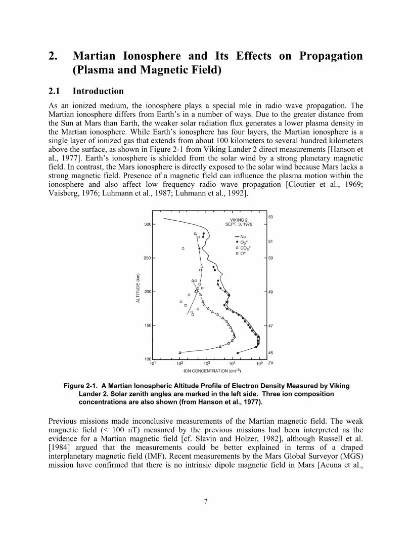
2.1 Introduction As an ionized medium, the ionosphere plays a special role in radio wave propagation. The Martian ionosphere differs from Earth’s in a number of ways. Due to the greater distance from the Sun at Mars than Earth, the weaker solar radiation flux generates a lower plasma density in the Martian ionosphere. While Earth’s ionosphere has four layers, the Martian ionosphere is a single layer of ionized gas that extends from about 100 kilometers to several hundred kilometers above the surface, as shown in Figure 2-1 from Viking Lander 2 direct measurements [Hanson et al., 1977]. Earth’s ionosphere is shielded from the solar wind by a strong planetary magnetic field. In contrast, the Mars ionosphere is directly exposed to the solar wind because Mars lacks a strong magnetic field. Presence of a magnetic field can influence the plasma motion within the ionosphere and also affect low frequency radio wave propagation [Cloutier et al., 1969; Vaisberg, 1976; Luhmann et al., 1987; Luhmann et al., 1992].

Figure 2-1. A Martian Ionospheric Altitude Profile of Electron Density Measured by Viking Lander 2. Solar zenith angles are marked in the left side. Three ion composition concentrations are also shown (from Hanson et al., 1977).

Previous missions made inconclusive measurements of the Martian magnetic field. The weak magnetic field (< 100 nT) measured by the previous missions had been interpreted as the evidence for a Martian magnetic field [cf. Slavin and Holzer, 1982], although Russell et al. [1984] argued that the measurements could be better explained in terms of a draped interplanetary magnetic field (IMF). Recent measurements by the Mars Global Surveyor (MGS) mission have confirmed that there is no intrinsic dipole magnetic field in Mars [Acuna et al.,

7

1998]. The MGS magnetometer discovered that the Martian magnetic field is very weak compared to that of Earth’s magnetic field, only 1/800 the strength. The weak magnetic field is probably generated by a diffused draping IMF. The solar wind rams into the Martian ionosphere and generates complicated magnetic fields. Thus, this region may have a complicated interaction with the Martian magnetosphere [Acuna et al., 1998; Vaisberg, 1976; Slavin et al., 1991; Woo and Kliore, 1991].

2.2 Formation of the Martian Ionosphere The extreme ultraviolet (EUV) radiation from the Sun creates the dayside ionosphere of Mars by photo-ionization of its upper atmosphere [McElroy et al., 1977; Fox and Dalgarno, 1979]. This can be described by an ideal Chapman layer, which is formed through the solar wind plasma interaction with a typical unmagnetized planet with atmosphere. The interaction process is shown in Figure 2-2, which is based on a combination of observations and theoretical calculations [Luhmann et al., 1987]. Since there is little or no intrinsic magnetic field on Mars, on dayside, the solar wind can directly interact with its ionosphere [Cloutier et al., 1969]. This forms an extensive comet-like induced magnetosphere, which generally stands off the solar wind well above the planet. The solar wind is shocked and diverted around the ionopause where its incident pressure is approximately balanced by the thermal pressure of the ionospheric plasma. The region between the bow shock and the obstacle is called the magnetosheath or planetsheath. The draped IMF piles up in the front of the ionosphere, forming a region called the “magnetic barrier” [Zhang et al., 1991]. The ions are picked up by the solar wind flow, and they in turn slow the solar wind flow. The shielding current carried by the Mars ionosphere can largely exclude IMF and solar wind plasma from altitudes below the ionopause. The ionopause is also a region of transition between the cold planetary plasma and the post-shocked hot solar wind plasma. This interface between the ionospheric plasma and the shocked solar wind surrounds the planet and extends several thousand kilometers downstream where it forms the ionotail in the nightside [Bauer and Hartle, 1973; Vaisberg and Smirnov, 1986]. When the upstream solar wind carries the IMF through the bow shock and magnetosheath to the obstacle, the field line either slips through or around the conducting ionosphere. This diversion and slowing of the flow, possibly enhanced by mass loading of the flow near the obstacle, causes the field lines to drape and form an ionotail. Since the ionosphere is a conductor, the magnetic field convecting with solar wind plasma generates currents in it that keep the field from penetrating through the Martian ionosphere. Eventually, however, the field diffuses into Mars on a time scale that depends on the ionosphere’s conductivity.

8

Figure 2-2. Illustration of the Steps that Lead to the Formation of the Mars Ionosphere in the Solar Wind and Interplanetary Magnetic Field (from Luhmann et al., 1987).

2.3 Dayside Martian Ionospheric Structure Most of the Mars ionospheric measurements were made through radio occultation experiments performed by Mars missions from the United States and the former Soviet Union during the past 30 years [Gringauz, 1976a and b; Hanson and Mantas, 1988; Kliore et al., 1966, 1969, and 1973; Kolosov, 1972]. The only in-situ ionospheric measurements were obtained by two Viking Landers [Hanson et al., 1977; Chen et al., 1978; Mantas and Hanson, 1987] and by MGS [Acuna et al., 1998]. During the Aerobraking phase, the MGS orbiter reached as low as 108 km in altitude, below the peak of the ionosphere. Figure 2-3 shows the measurements made by the MGS Electron Reflector and Magnetometer from its 5th orbit.

9

When the spacecraft approached Mars, there was a sudden increase in magnetic field associated with the bow shock crossing. Then, in the sheath region, the magnetic field was turbulent and the plasma strongly energized. When the spacecraft was close to the ionosphere, at about 1000 km above the Mars surface, it detected a magnetic pile-up (magnetic barrier) region. Plasma density also increased with decreasing altitude. At about 130 km altitude, the ionosphere reached its density peak. Below the ionosphere, the magnetic field was very low (~5 nT), ruling out the possibility of a planet-wide intrinsic magnetic field. However, occasionally, the MGS magnetometer detected magnetic anomalies as strong as 400 nT near the Martian surface (not shown in Figure 2-3). These small spatial scale anomalies indicated that there are some local magnetic or iron structures in the Mars crust. On the outbound pass, the spacecraft detected similar ionospheric features.

Statistical studies based on available data [Hantsch and Bauer, 1990] indicate that the dayside Martian ionosphere may be generally described using a simple Chapman layer model:

{ })]/)((exp/)(1[5.0exp)( HhhHhhNhN mmm −−−−−= (2-1)

where (2-2) km NN )(cos0 χ=

and χsecln0 Hhhm += (2-3)

where Nm is electron peak density, hm is peak height, χ is solar zenith angle (SZA), H is the scale height of the neutral constituents, and N0 and h0 are the peak electron density and the peak height over the zenith (χ = 0°).

For an ideal Chapman layer (k = 0.5), the ionosphere should be in photochemical equilibrium with both the neutral gas scale height H and the ionizing radiation flux constant [Ratcliffe, 1972]. The peak heights increase with increasing solar zenith angle toward the terminator. For the real dayside Mars ionosphere, it is found that k = 0.57 through a curve fitting [Zhang et al., 1990a]. This small departure from the ideal case is expected because the ionizable constituent and the scale height vary with solar zenith angle and solar activity.

Figure 2-4a shows the data and a best fit curve. The peak electron densities decrease with increasing SZA with a ±15% fluctuation. At 0° SZA, the N0 is expected to be 2×105 cm-3, even though low-zenith-angle (χ < 40°) measurements of the Martian ionospheric electron densities cannot be obtained with radio occultation. Another major factor in determining the ionospheric profile is the density peak height. Figure 2-4b shows the curve fit using hm = 120 + 10 ln secχ. The peak height is at about 120 km altitude. The Mariner 9 measurements are excluded from this fit because these data significantly departed from the group. High peak altitude values measured in the Mariner 9 mission were caused by the 1971 great Mars global dust storm [Kliore et al., 1973; Stewart and Hanson, 1982]. This global dust storm appears to have elevated the Martian ionosphere as a whole by ~20–30 km without otherwise notably altering its density profile. The heating of the Martian atmosphere by the dust storm enhanced ionospheric scale height and peak height. McElroy et al. [1977] were able to model this behavior by assuming that a 20-K increase in temperature was followed by a steady cooling (8 K/6 weeks).

10

Figure 2-3. Electron and Magnetic Field Observations for MGS Day 262 (Orbit 5). Electron fluxes are shown as line traces at five energies (upper panel) and as a spectrogram (second panel) with the relative density of cold (<10 eV) electrons superimposed by using the same number of logarithmic intervals as the spectrogram's energy scale. The next three panels show the magnetic field amplitude, and the root mean square (RMS), and the spacecraft altitude. Vertical lines indicate the locations of the bow shock (BS), magnetic pile-up boundary (MPB), and ionospheric main peak (Nm) (from Acuna et al., 1998).

Figure 2-4. Peak Electron Densities and Peak Altitudes of the Mars Ionosphere. (a) Peak

electron densities of the Mars ionosphere as a function of solar-zenith angle; (b) Peak altitudes versus solar-zenith angle (from Hantsch and Bauer, 1990).

11

In the lower ionosphere, photoelectron ionization is significant and makes a contribution of 20–30% to the total ionization rate [Nier and McElroy, 1977]. Even though CO2 is the major atmospheric constituent of Mars at low altitudes and CO2

+ ions are the primary ions produced below 100 km, O2

+ ions are dominant at low altitudes because most of the CO2+ ions are broken

down into O2+ ions through a subsequent ion-neutral reaction (C ). Ion

composition profiles and temperature are showed in Figure 2-5a and 2-5b [Shinagawa and Cravens, 1989].

O2+ + O → O2

+ + CO

Because previous Mars missions covered more than three solar cycles, the maximum electron density as a function of solar radio flux has been studied from all data [Bauer and Hantsch, 1989; Hantsch and Bauer, 1990]. The peak density can change from 1.0×105 cm-3 at the solar minimum to 2.5×105 cm-3 at the maximum [Bauer and Hantsch, 1989]. At solar maximum, the topside ionospheric profile usually has large variations. There is an upper boundary, the ionopause, where solar wind dynamic pressure reaches a balance with the ionospheric thermal pressure and the plasma density falls sharply. When the ionopause is high, there is a fairly large plasma scale height (several hundred kilometers) below the ionopause. The topside ionospheric profile responds sensitively to incident solar wind pressure (and to a lesser extent to changes in the solar EUV flux). In contrast, at the solar minimum, the ionosphere constantly falls off with a small scale height (~20 km), and the ionosphere does not show such a response because the ionopause is within the deep region dominated by photochemistry (below ~225 km). On the basis of the past 30 years of measurements, the dayside Mars ionopause (the upper boundary of the ionosphere) locations detected during various solar cycle are shown in Figure 2-6 [Slavin and Holzer, 1982]. In comparison, the Martian obstacle location (which is inferred from the bow shock shape) is also displayed. The lower limit at solar minimum in 1965 was nearly 250 km from Mariner 4, and the upper limit at solar maximum was almost 400 km. No large solar zenith angle dependence has been seen in the Martian upper ionosphere.

Figure 2-5. Martian Ionospheric Plasma Density and Temperature Profiles. (a) Comparison of the calculated ion density profiles (solid lines from Shinagawa and Cravens, 1989) with Viking 1 and 2 measured profiles (Hanson et al., 1977); (b) Altitude profiles of ion, electron, and neutral temperatures.

12

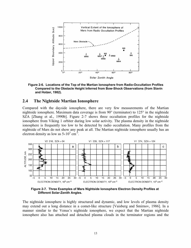
Figure 2-6. Locations of the Top of the Martian Ionosphere from Radio-Occultation Profiles Compared to the Obstacle Height Inferred from Bow-Shock Observations (from Slavin and Holzer, 1982).

2.4 The Nightside Martian Ionosphere Compared with the dayside ionosphere, there are very few measurements of the Martian nightside ionosphere. Maximum data coverage is from 90° (terminator) to 125° in the nightside SZA [Zhang et al., 1990b]. Figure 2-7 shows three occultation profiles for the nightside ionosphere from Viking 1 orbiter during low solar activity. The plasma density in the nightside ionosphere is frequently too low to be detected by radio occultation. Many profiles from the nightside of Mars do not show any peak at all. The Martian nightside ionosphere usually has an electron density as low as 5×103 cm-3.

Figure 2-7. Three Examples of Mars Nightside Ionosphere Electron Density Profiles at Different Solar-Zenith Angles.

The nightside ionosphere is highly structured and dynamic, and low levels of plasma density may extend out a long distance in a comet-like structure [Vaisberg and Smirnov, 1986]. In a manner similar to the Venus’s nightside ionosphere, we expect that the Martian nightside ionosphere also has attached and detached plasma clouds in the terminator regions and the

13

ionosphere has some rays, density holes, and filament structures in the anti-sunward tail region [Gringauz, 1976a and b]. The nightward plasma flow from dayside across the terminators is the main source of the nightside ionosphere due to the large day-to-night pressure gradients. This cross-terminator flow strongly depends on solar wind pressure. During the solar minimum, the transport source is cut off. However, near solar maximum, high solar wind pressure can also sometimes suppress the altitude of dayside ionopause over the terminator, reducing the normal nightward transport. Horizontal transport from dayside is possible because Mars has almost no intrinsic magnetic field, which could inhibit plasma flow across the terminator. Local ion production by energetic electron impact is another important source. However, because of the lack of solar wind data during Mars nightside ionospheric observations, we do not know which mechanism is more important.

2.5 Ionospheric Effects on Radio Wave Propagation We have plotted the dayside ionospheric density profiles for various values of SZA (χ) in Figure 2-8, using an average Martian dayside ionospheric model (Equation 2-1) and the following parameters: N0 = 2×105 cm-3, h0 = 125 km, H = 11 km, k = 0.57. The F2 layer of Earth’s ionosphere has a peak density of 2×106 cm-3 (2×1012 m-3) at dayside and a peak altitude of ~300 km. The Martian ionospheric plasma density is one order of magnitude lower than Earth’s, as shown in Table 2-1. The Martian dayside ionosphere at solar maximum has a peak density similar to that of the Earth nightside ionosphere at solar minimum. By integrating the dayside ionospheric profile, the total vertical electron content (TEC) of 4.0×1011/cm2 is obtained. This value is 50 times lower than Earth’s ionospheric TEC. Even though the Martian ionospheric peak density and TEC are lower than in the Earth’s ionosphere, we can still use them for ionospheric communication.

The Martian ionosphere can definitely be useful in future Mars ground-to-ground low-frequency communication. The Mars ionosphere can be used to perform trans-horizon (or beyond line of sight) communication for future Martian colonies, vehicles, and robots released from Mars

landers. The Martian ionospheric critical frequency, )(100.9)( 30

60

−−×= mNMHzf , is ~4.0 MHz for vertical incidence, which is a factor of 3 less than Earth’s ionospheric critical frequency. For an oblique incident wave, the usable critical frequency f0 = 4.0 (MHz) / cos θ0, where θ0 is the initial wave launch angle. Usable critical frequencies and single-hop distances, as a function of launch angle θ0, are listed in Table 2-2. Hop distance (l) is a function of wave launch angle and ionospheric height (h) l = 2 h tan θ0. When θ0 increases, the maximum usable critical frequencies for oblique propagation increase significantly. The frequency is high enough to carry useful information. Figure 2-9 shows schematically how the Martian ionosphere can be used as a reflector for global communication. As noted earlier, the prevalent Martian sand storms have significant effects on the ionospheric peak height. For example, the 1971 global dust storm increased the peak height by 20–30 km. An increase in peak height (∆h) will cause an increase in hop distance. This is equivalent to an enhancement in hop distance by ∆l = 2 ∆h tan θ0.

14

Figure 2-8. The Calculated Martian Dayside Ionospheric Altitude Profiles for Different Solar-Zenith Angles Using Equation 2-1 (Chapman layer model).

Table 2-1. Ionospheric Peak Density and Critical Frequency for Mars and Earth

Mars Earth Ionospheric Condition n0 (cm-3) f0 (MHz) n0 (cm-3) f0 (MHz)

Dayside Solar Max. 2.5x105 4.5 2.0x106 12.7

Solar Min. 1.0x105 2.9 5.0x105 6.3

Nightside* Solar Min. 5.0x103 0.6 2.0x105 4.0

Dayside TEC 4.0x1011 cm-2 2.0x1013 cm-2

* There is no nightside ionospheric data available for Mars during solar maximum.

15

Table 2-2. Usable Critical Frequency and Hop Distance for Various Launch Angles

Launch Angle θ0

0° 15° 30° 45° 60° 75°

Maximum Usable Frequency (MHz)

4.0 4.14 4.62 5.66 8.0 15.5

One Hop Distance (km) 0 67.0 144.3 250.0 433.0 933.0

Peak

hei

ght=

125k

m

Mars Ionosphere

Mars Surface

Figure 2-9. The Dayside Martian Ionosphere May Be Used as a Reflector for Trans-horizon Surface-to-Surface Communication. The maximum hop distance and usable frequency depend on the ray launch angles. Using this technique, one can keep in touch with areas beyond the line of sight.

The Martian dayside ionosphere has a stable peak density and peak height. During the solar maximum, N0 can reach 2.5×105 cm-3 (4.5 MHz in f0), while at solar minimum, there is a N0 of ~1.0×105 cm-3 (2.85 MHz in f0). The ionospheric peak height is between 120 and 130 km. The stable condition is favorable to oblique incident communication using the ionosphere as a reflector from Martian surface to surface. The nightside ionosphere has very low plasma density (~5×103 cm-3, corresponding to 0.63 MHz in f0). A model for the nightside ionosphere is not available yet. More measurements and analyses need to be done for the nightside ionosphere under different solar conditions. The nightside ionospheric profile often shows no dominant density peak and has large variations. Because of the low usable frequency and very unstable condition, the nightside ionosphere is unlikely to be useful for global communication.

Because of the relatively low maximum density, based on the term in Equation (1-1), the Martian ionospheric refractive index only significantly affects low frequency waves with frequencies below 450 MHz. The Martian ionosphere may slightly affect UHF links between a Mars lander (or rover) and an orbiter. Below 4.5 MHz, the cut-off frequency, the waves cannot pass through the ionosphere. The Martian ionosphere is almost transparent for radio waves with frequencies above 450 MHz. Because Mars has very little magnetic field (~50 nT), the term Y=

20 )/( ffX =

16

(fB / f) also has little effect to the radio waves. The average gyrofrequency is about 1.5 kHz. The gyrofrequency has almost no effect on waves above 1 MHz.

The plasma collision frequency in the low ionosphere, ν, remains unknown, but it should depend on both plasma and neutral temperature and density. This frequency is estimated to be below 1.0 kHz. This term can cause low frequency wave attenuation within the ionosphere through the image part of Z = (ν/f). The scintillation effects of the Martian ionosphere on radio waves are not yet known. We expect that there are more plasma irregularities in the nightside ionosphere. Such irregularities can cause fluctuations in both amplitude and phase for low-frequency radio signals.

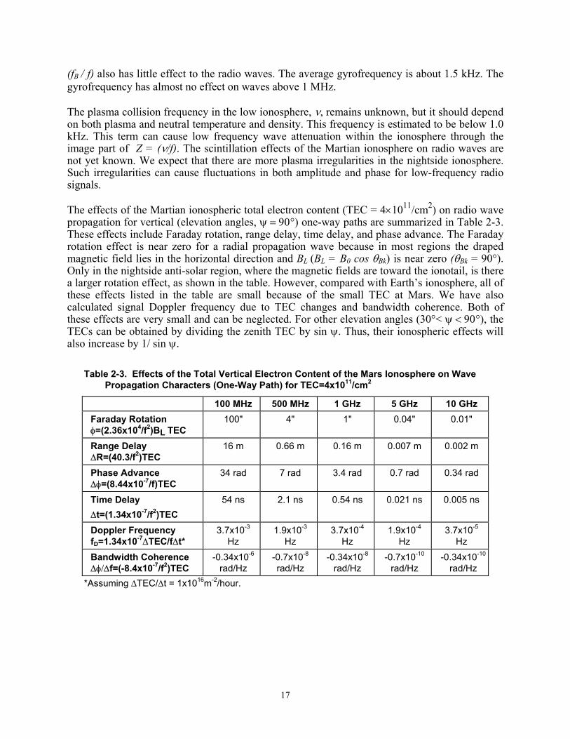
The effects of the Martian ionospheric total electron content (TEC = 4×1011/cm2) on radio wave propagation for vertical (elevation angles, ψ = 90°) one-way paths are summarized in Table 2-3. These effects include Faraday rotation, range delay, time delay, and phase advance. The Faraday rotation effect is near zero for a radial propagation wave because in most regions the draped magnetic field lies in the horizontal direction and BL (BL = B0 cos θBk) is near zero (θBk = 90°). Only in the nightside anti-solar region, where the magnetic fields are toward the ionotail, is there a larger rotation effect, as shown in the table. However, compared with Earth’s ionosphere, all of these effects listed in the table are small because of the small TEC at Mars. We have also calculated signal Doppler frequency due to TEC changes and bandwidth coherence. Both of these effects are very small and can be neglected. For other elevation angles (30°< ψ < 90°), the TECs can be obtained by dividing the zenith TEC by sin ψ. Thus, their ionospheric effects will also increase by 1/ sin ψ.

Table 2-3. Effects of the Total Vertical Electron Content of the Mars Ionosphere on Wave Propagation Characters (One-Way Path) for TEC=4x1011/cm2

100 MHz 500 MHz 1 GHz 5 GHz 10 GHz Faraday Rotation φ=(2.36x104/f2)BL TEC

100" 4" 1" 0.04" 0.01"

Range Delay ∆R=(40.3/f2)TEC

16 m 0.66 m 0.16 m 0.007 m 0.002 m

Phase Advance ∆φ=(8.44x10-7/f)TEC

34 rad 7 rad 3.4 rad 0.7 rad 0.34 rad

Time Delay ∆t=(1.34x10-7/f2)TEC

54 ns 2.1 ns 0.54 ns 0.021 ns 0.005 ns

Doppler Frequency fD=1.34x10-7∆TEC/f∆t*

3.7x10-3 Hz

1.9x10-3 Hz

3.7x10-4 Hz

1.9x10-4 Hz

3.7x10-5 Hz

Bandwidth Coherence ∆φ/∆f=(-8.4x10-7/f2)TEC

-0.34x10-6 rad/Hz

-0.7x10-8 rad/Hz

-0.34x10-8 rad/Hz

-0.7x10-10 rad/Hz

-0.34x10-10

rad/Hz *Assuming ∆TEC/∆t = 1x1016m-2/hour.

17

2.6 Summary and Recommendations The dayside ionosphere of Mars is generated through the photo-ionization of its upper atmosphere. The height of the ionosphere (ionopause) is dependent on solar wind pressure. A comet-like structure with low electron density extends several thousand kilometers at nightside.

The Martian dayside ionosphere may be described using a simple Chapman layer model. The ionosphere has a stable peak height and peak density. Its peak height is between 120 and 130 km. Martian dust storms significantly increase the ionospheric peak height. On average, the dayside Martian ionospheric plasma density is one order of magnitude lower than Earth’s. Its TEC value is 50 times lower than Earth’s ionospheric TEC.

The plasma density in the nightside ionosphere is very low (5 ×103 cm3 ). The nightward plasma flow from dayside crossing the terminators is the main plasma source for the nightside ionosphere. The nightside ionospheric profile often shows no dominant density peak and has large variations.

Recommendation: The Martian ionosphere may play an important role in future Mars ground-to-ground global communications. The Martian dayside ionospheric critical frequency is ~ 4.0 MHz for vertical incidence. This frequency is high enough to carry useful amounts of data. The stable conditions in the dayside ionosphere are favorable for oblique-incidence communication using the ionosphere as a reflector for Martian surface-to-surface communication. Usable critical frequency and hop distance for an oblique-incidence wave significantly increase with the wave launch angle. Using the Martian ionosphere, we can also perform trans-horizon (or beyond line-of-sight) long-range communication for future Martian colonies, rover vehicles, and robots released from Mars landers. However, the nightside ionosphere has some limitations for global communication because of its low usable frequency and very unstable conditions.

The Martian ionosphere only effects the low frequency waves with frequencies below 450 MHz. Below 4.5 MHz, the cut-off frequency, the waves cannot pass through the ionosphere. It is almost transparent for radio waves with frequencies above 450 MHz. Because Mars has very little magnetic field (~ 50 nT), its gyrofrequency (fB) has almost no effect on waves with frequencies above 1 MHz.

References

Acuna, M.H., et al., Magnetic field and plasma observations at Mars: Initial results of the Mars Global Surveyor Mission, Science, 279, 1676, 1998.

Bauer, S.J. and M.H. Hantsch, Solar cycle variation of the upper atmosphere temperature of Mars, Geophys. Res. Lett., 16, 373, 1989.

Bauer, S.J., and R.E. Hartle, On the extent of the Martian ionosphere, J. Geophys. Res., 78, 3169, 1973.

Chen, R.H., et al., The Martian ionosphere in light of the Viking observations, J. Geophys. Res., 83, 3871, 1978.

18

Cloutier, P.A., et al., Modification of the Martian ionosphere by the solar wind, J. Geophys. Res., 74, 6215, 1969.

Fox, J. L. and A. Dalgarno, Ionization, luminosity, and heating of the upper atmosphere of Mars, J. Geophys. Res., 84, 7315, 1979.

Gringauz, K.I., Interaction of solar wind with Mars as seen by charged particle traps on Mars 2, 3, and 5 satellite, Rev. Geophys., 14, 391, 1976a.

Gringauz, K.I., On the electron and ion components of plasma in the antisolar part of near-Martian space, J. Geophys. Res., 81, 3349, 1976b.

Hantsch, M.H. and S.J. Bauer, Solar control of the Mars Ionosphere, Planet Space Sci., 38, 539, 1990.

Hanson, W.B., and G.P. Mantas, Viking electron temperature measurements: Evidence for a magnetic field in the Martian ionosphere, J. Geophys. Res., 93, 7538, 1988.

Hanson, W.B., S. Sanatani, and D.R. Zuccaro, The Martian ionosphere as observed by the Viking retarding potentail analyzers, J. Geophys. Res., 82, 4351, 1977.

Kliore, A.J. et al, Radio occultation measurement of the Martian atmosphere over two regions by the Mariner IV space probe, Moon and planets, Edited by Dollfus, A., 226, North-Holand, Amsterdam, 1966.

Kliore, A.J., et al., Mariners 6 and 7: Radio occultation measurements of the atmosphere of Mars, Science, 166, 1393, 1969.

Kliore, A.J., D.L. Cain, G. Fjeldbo, B.L. Seidel, M.J. Sykes, and S.I. Rasool, The atmosphere of Mars from Mariner 9 radio occultation measurements, Icarus, 17, 484, 1972.

Kliore, A.J., et al., S Band radio occultation measurements of the atmosphere and topography of Mars with Mariner 9: Extended mission coverage of polar and intermediate latitude, J. Geophys. Res., 78, 4331, 1973.

Kolosov, M.A., Preliminary results of radio occultation studies of Mars by means of the Orbiter Mars 2, Dokl. Akad. Nauk SSSR, 206, 1071, 1972.

Luhmann, J.G., et al., Characteristics of the Mars-like limit of the Venus-solar wind interaction, J. Geophys. Res ., 92, 8545, 1987.

Luhmann, J.G., et al., The intrinsic magnetic field and solar-wind interaction of Mars, in Mars, edited by H.H. Kieffer et al., The University of Arizona Press, Tucson & London, 1090, 1992.

Mantas, G.P., and W.B. Hanson, Analysis of Martian ionosphere and solar wind electron gas data from the planar retarding potential analyzer on the Viking spacecraft, J. Geophys. Res., 92, 8559, 1987.

McElroy, M.B., et al., Photochemistry and evolution of Mars’ atmosphere: A Viking perspective, J. Geophys. Res., 82, 4379, 1977.

Nier, A.O., and M.B. McElroy, Composition and structure of Mars’ upper atmosphere: Results from the neutral mass spectrometers on Viking 1 and 2, J. Geophys. Res., 82, 4341, 1977.

Ratcliffe, J.A., An Introduction to the Ionosphere and Magnetosphere, Cambridge University Press, New York, 1972.

19

Russell, C.T., et al., The magnetic field of Mars: Implications from gas dynamic modeling, J. Geophys. Res., 98, 2997, 1984.

Shinagawa, H. and T.E. Cravens, A one-dimensional multispecies magnetohydrodynamic model of the dayside ionosphere of Mars, J. Geophys. Res., 94, 6506, 1989.

Slavin, J.A., and R.E. Holzer, The solar wind interaction with Mars revisited, J. Geophys. Res., 87, 10285, 1982.

Slavin, J.A., et al., The Martian magnetosphere: Phobos 2 observations, J. Geophys. Res., 96, 11235, 1991.

Stewart, A.I., and W.B. Hanson, Mars upper atmosphere: Mean and variations, the Mars reference atmosphere, Ed. by Kliore, A.J., Adv. Space Res., 2, 2, 1982.

Vaisberg, O.L., Mars-plasma environments, in Physics of Solar Planetary Environments, Edited by D.J. Williams, 854, AGU, Washington, D.C., 1976.

Vaisberge, O., and V. Smirnov, The Martian magnetotail, Adv. Space Res., 6, 301, 1986. Woo, R., and A. Kliore, Magnetization of the ionosphere of Venus and Mars, J. Geophys. Res.,

96, 11073, 1991. Zhang, M.H.G., et al., A post-Pioneer Venus reassessment of the Martian dayside ionosphere as

observed by radio occultation methods, J. Geophys. Res., 95, 14829, 1990a. Zhang, M.H.G., J.G. Luhmann, and A.J. Kliore, An observational study of the nightside

ionospheres of Mars and Venus with radio occultation methods, J. Geophys. Res., 95, 17095, 1990b.

Zhang, T.L., et al., Magnetic barrier at Venus, J. Geophys. Res., 96, 11145, 1991.

20