2 Oxford Tidal Energy Workshop - Home — Department of …€¦ · · 2013-07-29Proceedings of the 2nd Oxford Tidal Energy Workshop (OTE 2013) ... 14:50 The Effects of Wave-Current

Proceedings of the

2nd Oxford Tidal Energy Workshop

18-19 March 2013, Oxford, UK

Proceedings of the 2nd Oxford Tidal Energy Workshop (OTE 2013)


Monday 18th March Session 1: Device Scale Problems (1) 11:10 CFD predicted effect of EMEC velocity profiles on a tidal stream turbine

James McNaughton (University of Manchester) 3 11:35 Validation of an Actuator Line Model for Tidal Turbine Simulations

Justine Schluntz (University of Oxford) 5 12:00 Hydrodynamics of tidal-stream turbines in unsteady flow

Duncan M. McNae (Imperial College London) 7 12:25 Influence of support structure response on extreme loading of a tidal turbine

due to turbulent flow and waves E. Fernandez Rodriguez (University of Manchester) 9

Session 2: Turbulence and Waves 14:00 Examination of Turbulence Characteristics Calculated Using the Variance Method

Michael Togneri (Swansea University) 11 14:25 Analysis of length scales in open channel flow for inlet definition of LES of tidal

stream turbines S. Rolfo (University of Manchester) 13

14:50 The Effects of Wave-Current Interactions on the Performance of Horizontal Axis

Tidal-Stream Turbines Tiago A. de Jesus Henriques (University of Liverpool) 15

Session 3: Array Scale Problems 15:45 Adjoint based optimisation of turbine farm layouts

Stephan C. Kramer (Imperial College London) 17 16:10 Impact of tidal energy arrays located in regions of tidal asymmetry

Simon P. Neill (Bangor University) 19 16:35 Beyond the Betz Theory - Blockage, Wake Mixing and Turbulence

Takafumi Nishino (University of Oxford) 21 Tuesday 19th March Session 4: Geographic Scale Problems 9:30 On the optimum place to locate a tidal fence in the Severn Estuary

Scott Draper (University of Western Australia) 23 9:55 Tidal Stream Energy Assessment of the Anglesey Skerries

Sena Serhadlıoğlu (University of Oxford) 25 10:20 Influence of tidal energy extraction on fine sediment dynamics

Peter E. Robins (Bangor University) 27

Session 5: Device Wake, Interaction and Environment 11:10 On the performance of axially aligned tidal stream turbines using a Blade Element

Disk approach Ian Masters (Swansea University) 29 11:35 Characterisation of the near-wake of a Horizontal Axis Tidal Stream Turbine in

Non-uniform steady flow Siân C. Tedds (University of Liverpool) 31

12:00 Tidal Turbine Wake Recovery due to Turbulent Flow and Opposing Waves

Alex Olczak (University of Manchester) 33 12:25 Individual Based Modelling Techniques and Marine Energy

Thomas Lake (Swansea University) 35 Session 6: Device Scale Problems (2) 13:40 CFD Analysis of a Single MRL Tidal Turbine

Matthew Berry (University of Exeter) 37 14:05 Numerical Modelling of a Laboratory Scale Tidal Turbine

Robert M. Stringer (University of Bath) 39 14:30 Progress on Large Vertical Axis Tidal Stream Rotors Stephen Salter (University of Edinburgh) 41 14:55 Comparisons of computational predictions and experimental measurements of ducted

tidal turbine performance Conor F. Fleming (University of Oxford) 43 Poster presentations: Investigating the Impacts of renewable on Coastal Hydrodynamics and Sediment Transport

Daniel Eddon (University of Liverpool) 45

Impact of wind variability on marine current turbines Alice J. Goward Brown (Bangor University) 47 The importance of inter-annual variability in assessing the environmental impact of tidal energy schemes

Matt Lewis (Bangor University) 49 Workshop Organisers: Richard H. J. Willden (Chairman) - University of Oxford Takafumi Nishino (Co-Chairman) - University of Oxford Scientific Committee: T. A. A. Adcock (Oxford) T. Stallard (Manchester) G. T. Houlsby (Oxford) P. K. Stansby (Manchester) I. Masters (Swansea) R. H. J. Willden (Oxford) T. Nishino (Oxford)

2nd Oxford Tidal Energy Workshop 18-19 March 2013, Oxford, UK

CFD predicted effect of EMEC velocity profiles on a tidal stream turbine

James McNaughton1, Stefano Rolfo School of MACE, University of Manchester, M13 9PL, UK

David Apsley, Tim Stallard, Peter Stansby

School of MACE, University of Manchester, M13 9PL, UK

Summary: This work investigates the predicted effects of realistic tidal conditions on a 1MW tidal stream turbine (TST) using EDF's open-source CFD solver, Code_Saturne. The turbine is to be installed at the European Marine Energy Centre (EMEC) in Orkney. A strongly sheared profile is employed to represent flood tide and a roughly parabolic profile, with maximum just below hub height, to represent ebb tide. The effect of these different flow conditions are assessed through instantaneous and mean quantities of power and thrust coefficients.

Introduction

Computational Fluid Dynamics (CFD) simulations of tidal stream turbines provide an opportunity for detailed analysis of turbine design changes at a reduced cost of both time and money when compared to experimental approaches. Whilst CFD cannot replace laboratory or field-scale experiments it is not always possible to examine specific conditions by physical experiment or to obtain high resolution flow or loading information that is often desirable for design. For these reasons, provided that confidence is given in the CFD results, such studies are an important contribution towards the tidal industry. Here analysis is presented for a full-scale three-bladed 18m diameter horizontal axis 1MW TST in a channel of 43m depth.

Methods

Results are obtained using Reynolds Averaged Navier Stokes (RANS) modelling with EDF's open-source CFD solver, Code_Saturne [1]. The k-ω-SST turbulence model is used after an investigation of suitable models and numerical methods [2] which compares to a 0.8m experimental TST [3]. Three velocity profiles, shown in Fig. 1, are selected to model the flow: Uniform, Flood and Ebb. These are selected from curve-fitting to field data provided as part of the project. All profiles have approximately the same depth averaged velocity of 1.8 m/s although the bulk velocity through the turbine's swept area is increased by 2% and 3% for the Flood and Ebb profiles respectively. All modelled profiles have the same low (1%) turbulence intensity. This is not typical of flows at the EMEC test-site but is employed to isolate the effect of sheared profiles. Increased turbulence levels lead to the depth-varying profiles to re-establish into classical logarithmic profiles and so to consider the effect of increased turbulence levels a uniform profile with 10% turbulence intensity at the inlet is also presented.

Results

Instantaneous thrust and power coefficients for each of the three velocity profiles are shown in Fig. 2 over a full rotation, with θ=0° indicating that the blade is aligned vertically upward and: The velocity in the denominator is the bulk velocity through the turbine's swept area. This is defined as the average of the velocity prescribed at the inlet across the projected turbine area. For the uniform profile the force coefficients are almost constant over a rotation with minimums occurring due to blade passing the mast at 175° and 164° for the thrust and power coefficients respectively. The effect of the different velocity profiles causes a greater magnitude of fluctuations to the coefficients, with, as expected, maximum values at the depths where the velocity is greatest. The change of velocity profiles has almost no effect on the mean thrust coefficient. However, the power coefficient increases by 1.2% and 3% for the flood and ebb profiles respectively which is of a similar order to the increase in bulk velocity through the swept area. The effect of the increased turbulence intensity leads to an increase and decrease in thrust and power coefficients by 2% and 0.5% respectively. It is

1 Corresponding author. Email address: [email protected]

.2/1Power

2/1Thrust

23B

P22B

T πRρU=C,

πRρU=C


observed that in this case the increase in turbulence causes the minimum of the coefficients (due to the mast) to lag by 10° and 15° for thrust and power respectively. This fluctuation is also damped indicating that the mast may have less effect on the turbine’s performance in actual flow conditions. Results are also presented to show that the shear in both flood and ebb profiles is maintained in a two-dimensional representation of the full-scale channel without the presence of the TST. This is due to the choice of low inlet turbulence and a length-scale that is comparable to the turbine hub-height.

Conclusions

Results from four turbulent velocity profiles are analysed to predict the effect of flow conditions typical of the EMEC test site on an 18m diameter TST. Instantaneous force coefficients are sensitive to the depth-varying velocity, although the mean thrust coefficient is not affected and the mean power coefficient increases with bulk velocity through the turbine's swept area. The sensitivity of the uniform flow to the mast is reduced by the effect of increased turbulence levels. Further work investigates the effect of both constant and depth-varying yawed flow to further investigate the effects of the EMEC test site. Acknowledgements: This research was conducted as part of the Reliable Data Acquisition Platform for Tidal (ReDAPT) project commissioned and funded by the Energy Technologies Institute (ETI). The authors would also like to acknowledge the assistance given by IT services at The University of Manchester. References: [1] Archambeau, F., Mechitoua, N., and Sakiz, M. (2004). Code Saturne: a finite volume code for the

computation of turbulent incompressible flows-industrial applications. International Journal on Finite Volumes, 1(1):1–62.

[2] McNaughton, J., Rolfo, S., Afgan, I., Apsley, D.D., Stallard, T., Stansby, P.K. (2012). CFD prediction of

turbulent flow on an experimental tidal stream turbine using RANS modelling. In Proc. First Asian Wave and Tidal Energy Conference, Jeju Island, South Korea.

[3] Bahaj, A. S., Molland, A. F., Chaplin, J. R., and Batten, W. M. J. (2007). Power and thrust measurements

of marine current turbines under various hydrodynamic flow conditions in a cavitation tunnel and a towing tank. Renewable Energy, 32(3):407–426.

Fig. 1. (a) Velocity profiles used in this study. (b) Mean velocity on a vertical plane through the turbine’s centre-line.

Fig. 2. Instantaneous thrust and power coefficients resulting from different velocity profiles. Bulk velocity through turbine swept area is used to normalise coefficients.


Validation of an Actuator Line Model for Tidal Turbine Simulations

Justine Schluntz*, Richard H. J. Willden Department of Engineering Science, University of Oxford, OX1 3PJ, UK

Summary: A RANS-embedded actuator line model for tidal turbine simulation has been developed and validated using the NREL Phase VI wind tunnel experiments [1]. Actuator line models, first introduced by Sorensen and Shen [2] for wind turbine simulations, enable time resolved rotor simulations without requiring blade boundary layer discretisation. This results in a lower computational cost than blade resolved simulations whilst preserving the predominant features of the rotor wake. The present method uses a novel velocity sampling technique that circumvents the requirement for smearing techniques used in other actuator line models. The present model was validated through comparison of computed integrated loads and radial force coefficients with the NREL experimental results.

Introduction The NREL Phase VI wind turbine results are widely used in wind turbine model validation [3-5]. As there is no comprehensive high Reynolds number experimental data freely available for tidal turbine experiments, the Phase VI wind tunnel results were selected for comparison of the actuator line model.

A two-bladed, 10.058 m diameter horizontal-axis turbine was used in the Phase VI experiments. The NREL S809 aerofoil section was used from 0.25R to the blade tip and the blades were linearly tapered. Flow speeds ranged from 5 to 25 m/s and the turbine operated at 72 RPM. Pressure taps at 5 radial blade stations allowed for radial blade forces to be computed in addition to the rotor torque and root flap bending moment.

Methods The cross section of the computational domain was 24.4 m (4.85R) x 36.6 m (7.28R), in accordance with the wind tunnel dimensions. The domain extended 3R upstream of the turbine and 6R downstream of the turbine. The turbine shaft was explicitly included in the domain and the dimensions of this shaft matched the dimensions of that used in the experiment. A simplified nacelle was also explicitly included in the domain. The computational domain consisted of 1.35 x 106 cells. The rotor blades were simulated using actuator lines, each consisting of 60 collocation points in a cosine distribution. During each iteration, the flow velocity at each collocation point was determined using flow velocities sampled at 3 corresponding locations (above, upstream, and below the blade segment). The force on a corresponding spanwise blade segment was then calculated and input into the flow solver. Following convergence, the time was updated and the position of the actuator lines was adjusted accordingly. Simulations were performed for 6 wind speeds, representing tip speed ratios ranging from 1.51 to 5.41. The k-ω SST turbulence model was used in this study. A uniform velocity profile was set at the inlet of the domain. For each wind speed, the torque and root flap moment were calculated at each rotor position and averaged over a single revolution. The average radial force coefficients over a revolution were also calculated.

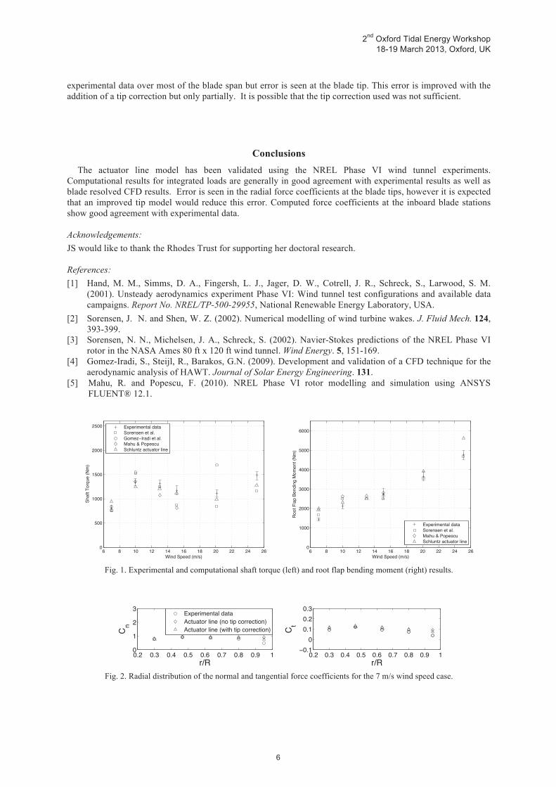
Results The actuator line results for integrated loads are shown in Figure 1 for each wind speed simulated. Also shown are the experimental results and results from several blade-resolved CFD studies selected for comparison. The actuator line results are generally in good agreement with the experimental results and are more accurate than the blade-resolved results for several wind speeds. The largest error for shaft torque occurs for the 7 m/s wind speed case (tsr = 5.41) and is 17%. There is also notable over-prediction of the root flap moment for the 7 m/s and 25 m/s wind speeds, although the over-prediction at 7 m/s is similar to the result from the blade resolved simulation of Mahu and Popscu [5]. The rotor is operating in highly stalled conditions for the 25 m/s case (tsr - 1.51) and it is possible the aerodynamic data at the corresponding high attack angles is inaccurate, resulting in incorrect calculated values for the force on the blade segments. The radial normal and tangential force coefficients for the 7 m/s case are presented in Figure 2. Results with and without a tip correction are provided. The computational results show good agreement with the

* Corresponding author. Email address: [email protected]


experimental data over most of the blade span but error is seen at the blade tip. This error is improved with the addition of a tip correction but only partially. It is possible that the tip correction used was not sufficient.

Conclusions The actuator line model has been validated using the NREL Phase VI wind tunnel experiments. Computational results for integrated loads are generally in good agreement with experimental results as well as blade resolved CFD results. Error is seen in the radial force coefficients at the blade tips, however it is expected that an improved tip model would reduce this error. Computed force coefficients at the inboard blade stations show good agreement with experimental data. Acknowledgements: JS would like to thank the Rhodes Trust for supporting her doctoral research. References: [1] Hand, M. M., Simms, D. A., Fingersh, L. J., Jager, D. W., Cotrell, J. R., Schreck, S., Larwood, S. M.

(2001). Unsteady aerodynamics experiment Phase VI: Wind tunnel test configurations and available data campaigns. Report No. NREL/TP-500-29955, National Renewable Energy Laboratory, USA.

[2] Sorensen, J. N. and Shen, W. Z. (2002). Numerical modelling of wind turbine wakes. J. Fluid Mech. 124, 393-399.

[3] Sorensen, N. N., Michelsen, J. A., Schreck, S. (2002). Navier-Stokes predictions of the NREL Phase VI rotor in the NASA Ames 80 ft x 120 ft wind tunnel. Wind Energy. 5, 151-169.

[4] Gomez-Iradi, S., Steijl, R., Barakos, G.N. (2009). Development and validation of a CFD technique for the aerodynamic analysis of HAWT. Journal of Solar Energy Engineering. 131.

[5] Mahu, R. and Popescu, F. (2010). NREL Phase VI rotor modelling and simulation using ANSYS FLUENT® 12.1.

6 8 10 12 14 16 18 20 22 24 26

0

1000

2000

3000

4000

5000

6000

Wind Speed (m/s)

Roo

t Fla

p B

endi

ng M

omen

t (N

m)

Experimental dataSorensen et al.Mahu & PopescuSchluntz actuator line

Fig. 1. Experimental and computational shaft torque (left) and root flap bending moment (right) results.

0.2 0.3 0.4 0.5 0.6 0.7 0.8 0.9 10

1

2

3

r/R

Cn

Experimental dataActuator line (no tip correction)Actuator line (with tip correction)

Fig. 2. Radial distribution of the normal and tangential force coefficients for the 7 m/s wind speed case.

Influence of support structure response on extreme loading of a tidal turbine due to turbulent flow and waves

Fernandez Rodriguez, E., Stallard, T. and Stansby, P.K. School of Mechanical, Aerospace and Civil Engineering, University of Manchester, M13 9PL

Summary: Preliminary analysis is presented of the influence of support structure flexibility on the extreme values of thrust experienced by a tidal turbine due to both turbulent flow and opposing waves. A statistical analysis of experimental measurements of rotor thrust indicate that thrust with a probability of occurrence 1 in a1000 (0.1%) is approx. 50% greater than mean thrust due to turbulent flow only. For waves with velocity amplitude of half the mean velocity, the 0.1% thrust increases to 100% greater than the mean thrust. Loading and surge response of a rotor plane supported by a flexible structure is subsequently predicted. The basis of this approach is a single degree of freedom model of the response of the rotor plane, in surge only. Excitation force is obtained by a BEM code and hydrodynamic damping based on published data for a porous disc [1]. Response is sensitive to the rotor plane damping coefficients employed but initial findings indicate dynamic response reduces 0.1% thrust due to waves by 15% relative to a rigid structure.

Introduction Extreme loads represent an important design criterion for any support structures and the magnitude of such

loads is a driver of capital cost. Reduction of extreme loads may therefore reduce cost and increase component life. Many of the prototype tidal stream turbines that have been developed are supported on rigid bed-connected structures. However, several systems have recently been proposed comprising one or more turbines supported on a floating, moored platform. The peak loading on such systems may be due to a combination of the loads on the immersed turbine, loads on the floating platform and the dynamic response of the coupled system. The aim of the present work is to evaluate the influence of the dynamic response of a support structure on the extreme loads experienced by a tidal stream turbine when subjected to a combination of turbulent flow and opposing waves. It is assessed whether dynamic response of the structure can be employed to reduce the magnitude of the extreme rotor loads.

Experimental Measurement of Rotor Thrust Tests are conducted in a flume of water depth , 40/1.5 long and 10/.9 wide without presence of single

rotor [2] of diameter 9/15 . The unsteady flow is developed with specified regular waves of wavelength 9 and amplitude of 1/22.5 opposing a uniform flow. Flow velocity is recorded at hub height using Nortek Vectrino+Acoustic Doppler Velocimeter (ADV) probes at mid depth and midspan at 200 Hz. Each of the flows considered have comparable mean velocity but with velocity amplitude up to half mean velocity.

Support Structure Dynamic Response The rotor plane is supported on a rigid rod that is pin-supported at a distance (1.77 ) above the rotor axis. The

rotor plane thus prescribes an arc of radius equal to the length of the supporting rod. Since the rod length is large relative to rotor diameter, this is approximated as surge of the rotor plane. Heave, roll, sway and pitch are assumed negligible. The equation of motion in surge is written as:

Eq. 1 Whererotor’s added mass structure added mass displacement in surgerotor’s damping structural damping velocityRestoring Structural stiffness coefficient Mass of structure acceleration

= Excitation force, presently rotor's thrust mass of turbine

For an oscillating rotor plane, the horizontal force or thrust is calculated with the relative velocity to the incident flow ( ), the disk area ( ) and thrust coefficient ( ) as

Eq. 2

Initial simulations employ damping and inertia coefficients ( ) for a porous disk [1] to predict force and response amplitude of rotor oscillation. Radiation damping force coefficients ( ) for a floating support structure are obtained by the diffraction method WAMIT and incorporated in the model to assess influence on extreme loads.

Extreme Values

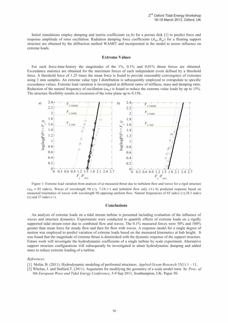
For each force-time-history the magnitudes of the 1%, 0.1% and 0.01% thrust forces are obtained. Exceedance statistics are obtained for the maximum forces of each independent event defined by a threshold force. A threshold force of 1.25 times the mean force is found to provide reasonable convergence of extremes using 3 min samples. An extreme value type I distribution is subsequently employed to extrapolate to specific exceedance values. Extreme load variation is investigated at different ratios of stiffness, mass and damping ratio.Reduction of the natural frequency of oscillation ( ) is found to reduce the extreme value loads by up to 15%.The structure flexibility results in excursion of the rotor plane up to 0.15 .

Figure 1: Extreme load variation from analysis of a) measured thrust due to turbulent flow and waves for a rigid structure

( .85 rads/s). Waves of wavelength 9 (□), 7.2 (+) and turbulent flow only (∗) b) predicted response based on measured kinematics of waves with wavelength 9 opposing uniform flow. Natural frequencies of 85 rads/s (□),38.3 rads/s (x) and 27 rads/s (○).

Conclusions

An analysis of extreme loads on a tidal stream turbine is presented including evaluation of the influence of waves and structure dynamics. Experiments were conducted to quantify effects of extreme loads on a rigidly supported tidal stream rotor due to combined flow and waves. The 0.1% measured forces were 50% and 100% greater than mean force for steady flow and then for flow with waves. A response model for a single degree of motion was employed to predict variation of extreme loads based on the measured kinematics at hub height. It was found that the magnitude of extreme thrust is diminished with the dynamic response of the support structure.Future work will investigate the hydrodynamic coefficients of a single turbine by scale experiment. Alternative support structure configurations will subsequently be investigated to attain hydrodynamic damping and added mass to reduce extreme loading of a turbine.

References:[1] Molin, B. (2011). Hydrodynamic modeling of perforated structures. Applied Ocean Research 33(1) 1 – 11.[2] Whelan, J. and Stallard,T. (2011). Arguments for modifying the geometry of a scale model rotor. In: Proc. of

9th European Wave and Tidal Energy Conference, 5-9 Sep 2011, Southampton, UK. Paper 50.

0 0.3 0.6 0.9 1.2 1.5 1.8 2.1 2.4 2.70

0.20.40.60.8

11.21.41.61.8

22.22.4

Fj /Fave

log(

log(P

(F<

=F j )) F1/100

F1/1000

F1/10000

0 0.3 0.6 0.9 1.2 1.5 1.8 2.1 2.4 2.70

0.20.40.60.8

11.21.41.61.8

22.22.4

Fj /Fave

log(

log(P

(F<

=F j ))

F1/1000

F1/10000

F1/100

b)a)

Examination of Turbulence Characteristics Calculated Using the Variance Method

Michael Togneri*, Ian Masters College of Engineering, Swansea University, Swansea, SA2 8PP

Summary: In this presentation we present and discuss various turbulence characteristics from selected high energy tidal sites, including turbulent kinetic energy density, Reynolds stress distributions and turbulent length scales. These characteristics are calculated using the variance method on data obtained using bed-mounted acoustic Doppler current profilers (ADCPs). We also perform some analysis of errors (i.e., bias and spread) in these quantities, and discuss the validity of the conventional techniques for quantifying these values. One site is found to have extremely intense turbulence on one phase of the tide, and we find that such circumstances appear to make the standard estimates of error less robust than is usually accepted.

Outline There are a great many difficulties involved in the design, installation and operation of tidal stream turbines (TSTs), not least of which is the action of turbulence on the installed device. Turbulence makes itself felt both through strong transient flow features leading to spikes in structural loading, and through additional fatigue load due both to the natural timescales of the turbulence itself and to 'eddy slicing', which intensifies fatigue loading at the rotational frequency and its harmonics. We hope that a deeper understanding of the turbulence processes in real marine flows will help us to improve predictions of structural load in a BEMT turbine performance model [1], and will also be useful in defining turbulent conditions for many of the other modelling approaches used in ocean energy, such as those discussed at the previous Oxford Tidal Conference [2].

Field measurements were obtained from three different sites, with peak flow velocities ranging from around 1-3 ms-1, using 4-beam ADCPs with high data collection frequencies. We begin by describing the techniques used to derive estimates of turbulence characteristics from subsets of this data; specifically, we examine periods of around an hour centred around the time of peak mean flow velocities during both flood and ebb phases. These results are then presented and discussed, with a particular emphasis on site-to-site comparison of results. Following on from this, we discuss how the errors in these estimates can be quantified, and some difficulties we have found with error estimation in strong turbulence.

Methods The conclusions that we can draw from ADCP data about the turbulence characteristics of the tidal stream depend strongly on the assumptions that we can safely make about the properties of the measured flow. The most fundamental assumptions are that the statistical properties of the flow are stationary for some suitable averaging period. and that they are spatially homogeneous across the beam spread of the device. Typically the averaging period is taken to be between 5 and 10 minutes; a 10-minute averaging period is used for all results presented here.

Most of the results presented depend on the use of the variance method, which is detailed in several places in the literature (see for instance Nystrom et al. [3], Lu and Lueck [4]). This method uses straightforward geometrical considerations in combination with statistical analysis of the along-beam velocities (which is the only information that can be directly obtained with an ADCP) to produce estimates of turbulence quantities in the water column above the measurement device. Some results obtained using this technique have been presented in [5]

Sample results We examine turbulence at three different sites, presenting our results as TKE densities, Reynolds stresses and turbulent lengthscales. At one of the three sites, we find that there is a strong flood-ebb asymmetry, with the turbulence characteristics on the ebb being fairly similar to results from other sites but the flood being far more turbulent. For instance, typically TKE density does not exceed 0.015 Jkg-1, whereas on the strongly turbulent flood values of up to 0.2Jkg-1 are observed. This increase in TKE is accompanied by an increase in the size of * Corresponding author. Email address: [email protected]

turbulent structures, as indicated by the integral lengthscales, which roughly double from approximately 5m on the ebb to 10m on the flood.

Figure 1 depicts variances and covariances of the squares of beam fluctuation velocities from a highly turbulent site. The standard error analysis techniques for the variance method assume that the individual beams of the ADCP have identical statistical properties (i.e., that Var(b3

'2) = Var(b4'2)), and that the cross-beam

covariance is negligibly small in comparison to the beam variances. While our results do indeed indicate that the beams' squared fluctuation variances are very similar to one another, we also see that the cross-beam covariance, although of lower magnitude than the individual variances, is not so much lower that it can be safely neglected. A straightforward reading of these results would change the variance of our Reynolds stress estimates by around 12%; however, we suggest that less restrictive assumptions are appropriate and allow us to use the original lower variance value for our stress estimates. Other results in the full presentation also indicate that the conventional error estimation techniques are not robust in highly turbulent conditions.

Acknowledgements: This work was undertaken as part of the Low Carbon Research Institute Marine Consortium (www.lcrimarine.org.uk), and as part of SuperGen UK Centre for Marine Energy Research (UKCMER). The authors wish to acknowledge the financial support of the Welsh Assembly Government, the Higher Education Funding Council for Wales, the Welsh European Funding Office and the European Regional Development Fund Convergence Programme. The authors would also like to acknowledge the support of EPSRC through grant EP/J010200/1, which funds the UKCMER project.

References: [1] Togneri, M., Masters, I., Orme, J. (2011). Incorporating turbulent inflow conditions in a blade element

momentum model of tidal stream turbines. ISOPE 2011. [2] Willden, R. et al (ed.) (2012). Extended Abstracts for Oxford Tidal Energy Workshop.[3] Nystrom, E.A., Rehmann, C.R., Oberg, K.A. (2007). Evaluation of Mean Velocity and Turbulence

Measurements with ADCPs. Journal of Hydraulic Engineering. 133(12), 1310-1318[4] Lu, Y., Lueck R.G. (1999). Using a Broadband ADCP in a Tidal Channel. Part II: Turbulence. Journal of

Atmospheric and Oceanic Technology. 16, 1568-1579 [5] Togneri, M., Masters, I. (2012). Comparison of turbulence characteristics for selected tidal stream power

extraction sites. ETMM 9.

Figure 1: Top two panels show variance in squares of velocity fluctuation for beams three and four;

lower panel shows cross-beam covariance of the same quantity. Data is taken from site three, duration of data record is approximately one hour.

2nd Oxford Tidal Energy Workshop18-19 March 2013, Oxford, UK

Analysis of length scales in open channel flow for inlet definitionof LES of tidal stream turbines

S. Rolfo,1 T. Stallard, J. McNaughton, D. Apsley, I. Afgan and P. StansbySchool of MACE, University of Manchester, M13 9PL, UK

Summary : The tidal streams considered for energy extraction are known to include strongly shearedvelocity profiles and large variation of flow speed due to both waves and eddies. One approach foranalysing turbine loading, due to such tidal flows, is eddy-resolved computational fluid dynamics. Akey issue with eddy-resolved methods is the specification and generation of an inflow that representsthe turbulence characteristics and flow-profile of a full-scale site. This paper addresses Large EddySimulation (LES) of both fully developed and developing open channel flow with the aim to evaluateturbulent lengthscales to compare with physical measurements from both lab and field scale data.

Introduction

In recent years the development of tidal stream turbines has received growing attention from both industryand academia as one of the possible alternative for energy production. Despite recent progress, thereremains limited understanding of the flow physics, particularly for the ambient conditions expected duringoperation. Computational Fluid Dynamics offers a potentially low cost approach for detailed investigationof such problems. Various methods may be employed. Recent examples of CFD of a fully resolvedturbine geometry include McNaughton et al. [1] and Afgan et al. [2]. These studies consider lab scaletidal stream turbine by means of several Reynolds Average Navier-Stokes (RANS) models and by LargeEddy Simulation (LES) respectively. Different turbulent intensities at the inlet have been studied, alongwith several tip speed ratios (TSR). One of the main conclusions drawn by this work is that turbineperformance (i.e. mean thrust and power) coefficients are comparable between RANS and LES at optimalTSR, whereas away from optimal point LES seems to give marginally better agreement with availableexperimental data. However, the eddy resolving method provides insight into both unsteady loads andthe detailed structure of the flow immediately downstream of the rotor. LES captures the blade tipvortices and the vortex shedding from the mast. The variation of the inlet turbulence intensity has alsoa important influence in the wake description, and particularly high levels of turbulence helps the wakerecovery. A very good description of the inlet turbulence is therefore mandatory and particularly theevaluation of the eddy length scale at different water depths. This information can be used to generaterepresentative inlet conditions for LES simulations using a Synthetic Eddy Method (SEM) [3].

Several simulations of open channel flow have been conducted at Reτ = 150, based on the frictionvelocity uτ and the water depth δ that corresponds to a Reynolds number ReB ≈ 2300 based on the bulkvelocity UB), in order to investigate the spatial variation of turbulent lengthscales, particularly the depthvariation, of both a fully developed flow and developing flow with and without a responding free surface.Higher Reynolds numbers, up to Reτ = 9300 (ReB ≈ 200k) where experimental data from Stallard etal. are available, have also been considered for comparison to experimental measurements of length-scaleobtained by two-point correlation at lab-scale. Initial comparisons are drawn for fully developed flow tovalidate a wall function approach for the near wall treatment. Further comparisons will be drawn fordeveloping profiles.

Numerical methods

Both wall resolved (i.e. down to the wall resolution) and wall modelled LES (i.e. wall function WF) havebeen performed using Smagorinsky model with van Driest damping of the turbulent viscosity (see Jarrinet al. [4] for details about LES with Code_Saturne). As a consequence of the different wall treatmentsseveral resolutions have been employed ranging from few hundred thousand control volumes, for very lowReynolds numbers or more high Re with WF, to some millions in case of wall resolved LES at moderateRe.Calculations have been performed using Code_Saturne, open-source CFD code developed by EDFR&D

1Corresponding author:Email address: [email protected]


100

101

102

0

5

10

15

20

DNSL

x=2π L

z=π

Lx=4π L

z=2π

(a)

y+ 100

101

102

0

0.1

0.2

0.3

0.4

0.5

0.6

0.7

0.8 (b)

y+0 0.2 0.4 0.6 0.8 1

0

0.5

1

1.5

2

2.5

3

(c)

y/δ

Figure 1: Mean velocity (a), shear stress τ12 (b) and rms stresses√τii for a open channel flow with rigid

lid at Ret = 150

0.7 0.8 0.9 1 1.1 1.2 1.3 1.40

0.2

0.4

0.6

0.8

1

lx=2π lz=π

lx=4π lz=2π

(a)

L11

y/δ

0 0.05 0.1 0.15 0.2 0.25 0.3 0.35 0.40

0.2

0.4

0.6

0.8

1

lx=2π lz=π

lx=4π lz=2π

(b)

L110.05 0.1 0.15 0.2 0.25 0.3 0.35 0.40

0.2

0.4

0.6

0.8

1

lx=2π lz=π

lx=4π lz=2π

(c)

L33

Figure 2: Turbulent lengthscales (a), L11 (streamwise) (b) L11 (spanwise) and (c) L33 (spanwise) foropen channel flow with rigid lid at Ret = 150

Results

Preliminary results are shown in Fig 1, where mean first and second order statistics from two wall resolvedLES at low Reynold number are compared with DNS. Mean velocity profiles and shear stress are all ingood agreement. The rms fluctuations of the normal stresses from LES are in excellent agreement withthe DNS in the near wall region, although different trends are observed close to the free surface. Thisdiscrepancy is a consequence of the kinematic condition which forces the vertical velocity to be zero andtherefore a redistribution of the fluctuations on the other two normal components of the Reynolds stresstensor. Fig. 2 shows different turbulent lengthscales in both streamwise and spanwise directions. Thetwo domain dimensions considered show very similar results for all components with the exception of L11

in the streamwise direction. This is a consequence of the very slow decay of the two point correlation ofstreamwise velocity fluctuations in the flow direction.

Further results involving higher Reynolds number and developing flow simulations will be presentedat the workshop, with a validation of the WF approach. The effect of a responding free surface will bealso investigated at the lower Reynolds number. Extension of developing flow and responding free surfacewill later be conducted up to Reτ = 65, 000, which is representative of the full-scale tidal flow.Acknowledgements: This research was conducted as part of the Reliable Data Acquisition Platform forTidal (ReDAPT) project commissioned and funded by the Energy Technologies Institute (ETI).References

[1] S. McNaughton, J.and Rolfo, I. Afgan, D.D. Apsley, T. Stallard, and P.K. Stansby. Cfd predictionof turbulent flow on an experimental tidal stream turbine using rans modelling. In First Asian Waveand Tidal Energy Conference, Jeju Island, South Korea, 2012.

[2] I Afgan, J.and McNaughton, D.D. Apsley, S. Rolfo, T. Stallard, and P.K. Stansby. Les of a 3-bladedhorizontal axis tidal stream turbine:comparisons to rans and experiments. In THMT12, Palermo,Italy, 2012.

[3] R Poletto, Alistair R, T Craft, and N Jarrin. Divergence free synthetic eddy method for embeddedLES inflow boundary conditions. In Seventh International Symposium On Turbulence and Shear FlowPhenomena (TSFP-7), Ottawa, 2011.

[4] N. Jarrin, S. Benhamadouche, D. Laurence, and R. Prosser. A synthetic-eddy-method for generatinginflow conditions for large-eddy simulations. International Journal of Heat and Fluid Flow, 27(4):585– 593, 2006.

The Effects of Wave-Current Interactions on the Performance of Horizontal Axis Tidal-Stream Turbines

Tiago A. de Jesus Henriques *, Avgi Botsari, Siân C. Tedds, Robert J. Poole, Hossein Najafian, Christopher J. Sutcliffe

School of Engineering, University of Liverpool, UK Ieuan Owen

School of Engineering, University of Lincoln, UK

Summary: An experimental investigation was performed using the high-speed re-circulating water flume at the University of Liverpool combined with a paddle wavemaker installed at the upstream of the working section to produce wave-current flow conditions. The set-up created reproducible and well characterized linear waves. A Vectrino plus Acoustic Doppler Velocimeter (ADV) system was used to measure three-dimensional velocity components through the water depth below two different waveforms. The experimental water particle velocity results obtained show an excellent agreement with theoretical results calculated using linear wave theory. For different flow conditions (current alone and wave-current interaction) power and thrust measurements were taken using athree bladed Horizontal Axis Tidal-Stream Turbine (HATT) (diameter = 0.5m).

Introduction

Wave–current flow fields can influence significantly the water particle velocity and therefore it’s necessary to understand the effects on thrust and power output of tidal devices. The elliptical motion of the water particle introduced by the presence of waves in the current can cause fluctuations on the power output which need to be considered in the design of turbine rotors. Furthermore the loading on the blades of the turbine will also be influenced by the changes in the water particle velocity since it will increase its maximum value and generate an additional cyclic loading which will determine life-time of the structure. Previous studies using a towing tank show that the presence of waves has a significant effect on both power and thrust and also waves cause fluctuations in the direction and magnitude of the forces acting on the blades [1, 2].

Experimental Methods The tests were carried out in the high-speed water channel (working section 1.4m wide, 3.7m long and 0.8m deep) capable of flow velocities between 0.03 and 6m/s with low turbulence intensity (TI) of approximately 2% [3]. The experimental work was performed using a three blade model of a HATT with a rotor diameter of 0.5m and an optimum blade pitch angle of 6o [3]. Regular waves were produced using a wavemaker which creates a wide range of wave-current flow conditions. The wavemaker consists of a hinged paddle, driven by an electric motor which as it rotates uses an adjustable throw crank to move the paddle up and down on the water surface to induce surface waves. The paddle spans the flume and it is aligned with the water surface in the working section. Wave frequency is adjustable between 0.7 – 2.7Hz and amplitude can be changed between 1 – 50mm using the variable throw yolk. The profiles of the waves generated in the working section were measured by means of aresistance probe which records changes in water surface elevation. For small amplitude and frequency settings the resulting wave pattern was well represented by a sine function and linear wave theory, from which the main wave characteristics (height, frequency and period) could be easily extracted. An Acoustic Doppler Velocimeter ((ADV) Nortek Vectrino+) was used to measure three-dimensional velocity components through the water depth below the waves. Measurements were taken at depths ranging from 0.15 to 0.525m from the Mean Water Level (MWL), thus covering the flow region within most of the turbine’s swept area. Using a sampling frequency of 200Hz samples with 500 waves (100,000 data points) were collected at each measurement location to ensure a 95% confidence interval [4]. The power and thrust coefficients of the tidal turbine under current alone and for different wave conditions were measured for a range of turbine torque settings.

ResultsFrom the range of waves produced it was chosen two different waveforms (waveform 1 - T=0.7s & length=1.4m; waveform 2 – T=0.9s & length=2m). The velocity components under the different waveforms * Corresponding author. Email address: [email protected]

studied was calculated using the linear wave theory as given by Dean & Dalrymple [5]. For both horizontal and vertical velocities the experimental measurements taken were found to have an excellent agreement with theoretical results as is shown in Figure1. The power and thrust coefficient (CP=P/[0.5ρAU3] & CT=T/[0.5ρAU2]) of the tidal turbine under current alone and current and wave combined was measured. The results, in Figure 2, show that the wave profiles studied have a limited effect on the average thrust power output of the turbine when compared with the results for current alone. However the standard deviation (σ) of both coefficients was significantly increased in the presence of waves.

Figure 1 - Horizontal & vertical water particle velocities for both waveforms

Figure 2 – Power and thrust coefficient under different flow conditions Conclusions

The experimental arrangement achieved allowed the creation of reproducible regular linear waves that showed a good agreement with linear wave theory. The fluctuating velocity components below the waves caused both power output and thrust to fluctuate significantly although with negligible effect on both arithmetic means. Acknowledgements: The technical assistance provided by Marc Bratley, Martin Jones and Derek Neary is gratefully acknowledged.

References: [1] Barltrop, N., Varyani, K.S., Grant, A., Clelland, D., Pham, X.P. (2007) Investigation into wave–current interactions in

marine current turbines., Journal of Power and Energy, pp. 233-242. [2] Galloway, P. W., Myers, L. E., Bahaj, A. S. (2010) Studies of a scale tidal turbine in close proximity to waves. s.n.,.

3rd International Conference on Ocean Energy, Bilbao, Spain. [3] Tedds, S.C., Poole, R.J., Owen, I., Najafian, G., Bode, S.P., Mason-Jones, A., Morris, C., O’Doherty, D.M.,

O’Doherty, T. (2011). Experimental Investigation Of Horizontal Axis Tidal Stream Turbines. In: Ninth European Wave and Tidal Energy Conference, Southampton, UK.

[4] Metcalfe, A.V. (1994) Statistics in Engineering. Chapman & Hall. London, U.K., Chapter 6. [5] Dean, R. G., Dalrymple, R. A. (1984) Water Wave Mechanics for Engineers and Scientists. Prentice-Hall, Inc. New

Jersey, U.S.A., Chapter 4.


Impact of tidal energy arrays located in regions of tidal asymmetry

Simon P. Neill School of Ocean Sciences, Bangor University, Menai Bridge LL59 5AB

Summary: Tidal stream turbines are exploited in regions of high tidal currents. Such energy extraction will alter the regional hydrodynamics, analogous to increasing the bed friction in the region of extraction. In addition, this study demonstrates that energy extracted with respect to tidal asymmetries due to interactions between quarter (M4) and semi-diurnal (M2) currents will have important implications for large-scale sediment dynamics. Model simulations show that energy extracted from regions of strong tidal asymmetry will have a much more pronounced effect on sediment dynamics than energy extracted from regions of tidal symmetry. This has practical application to many areas surrounding the UK, including the Irish Sea and the Bristol Channel, that exhibit strong tidal currents suitable for exploitation of the tidal stream resource, but where large variations in tidal asymmetry occur.

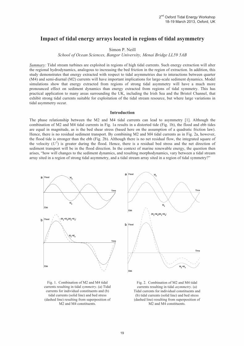
Introduction The phase relationship between the M2 and M4 tidal currents can lead to asymmetry [1]. Although the combination of M2 and M4 tidal currents in Fig. 1a results in a distorted tide (Fig. 1b), the flood and ebb tides are equal in magnitude, as is the bed shear stress (based here on the assumption of a quadratic friction law). Hence, there is no residual sediment transport. By combining M2 and M4 tidal currents as in Fig. 2a, however, the flood tide is stronger than the ebb (Fig. 2b). Although there is no net residual flow, the integrated square of the velocity (U

2) is greater during the flood. Hence, there is a residual bed stress and the net direction ofsediment transport will be in the flood direction. In the context of marine renewable energy, the question then arises, “how will changes to the sediment dynamics, and resulting morphodynamics, vary between a tidal stream array sited in a region of strong tidal asymmetry, and a tidal stream array sited in a region of tidal symmetry?”

Fig. 1. Combination of M2 and M4 tidal currents resulting in tidal symmetry. (a) Tidal

currents for individual constituents and (b) tidal currents (solid line) and bed stress

(dashed line) resulting from superposition of M2 and M4 constituents.

Fig. 2. Combination of M2 and M4 tidal currents resulting in tidal asymmetry. (a)

Tidal currents for individual constituents and (b) tidal currents (solid line) and bed stress

(dashed line) resulting from superposition of M2 and M4 constituents.


Methods A one-dimensional morphological model was developed and applied to a case study (the Bristol Channel) where large spatial variations in tidal asymmetry occur along the length of the channel. The morphological model consisted of three components: hydrodynamic, sediment transport and bed level change models [2]. An energy extraction term was incorporated into the hydrodynamic model, with power extracted as a function of U

3. The idealised power and power coefficient curves were based on a MCT ‘Seagen’ device [3]. The model was applied to the entire length of the Bristol Channel for a duration of 29.53 days (a lunar month), and the output for various energy extraction scenarios compared to the natural case.

Results The model results demonstrate that, regardless of the location of energy extraction, the magnitude of bed level change is dampened by the presence of a tidal stream farm (due to a general reduction in tidal velocity and hence net sediment transport). However, the location of energy extraction is important with regard to the magnitude of bed level change based on two main criteria: the magnitude of sediment transport at the point of extraction, and the degree of tidal asymmetry at the point of extraction. The first criterion is obvious, so the bed level change results were normalised by the gross mean sediment transport at the point of energy extraction, averaged over the duration of the simulation to remove the effect of longitudinal variations in the magnitude of sediment transport at the point of energy extraction. The main finding is that when energy is extracted from a region of strong tidal asymmetry, the effect on the resulting bed level change is more pronounced (up to 29% difference from the natural tidal channel case) compared with energy extracted from regions of tidal symmetry (18% difference).

Conclusions A one-dimensional numerical model has demonstrated that a small amount of energy extracted from a tidal system can lead to a significant impact on the sediment dynamics, depending on tidal asymmetry at the point of extraction. The resulting influence on the morphodynamics is not confined to the immediate vicinity of the tidal stream farm, as would occur in the case of localised scour, but affects the erosion/deposition pattern over a considerable distance from the point of energy extraction (of order 50 km in the case of the Bristol Channel). However, regardless of the location of a tidal stream farm within the tidal system, energy extraction reduces the overall magnitude of bed level change in comparison with non-extraction cases. Therefore, when considering the environmental impact of a large-scale tidal stream farm, it is important to consider the degree of tidal asymmetry in addition to the local magnitude of tidal currents at the point of energy extraction. References: [1] Pingree, R. D., Griffiths, D. K. (1979). Sand transport paths around the British Isles resulting from the M2 and M4 tidal interactions. J. Mar. Biol. Assoc. U.K. 59, 497-513. [2] Neill, S. P., Litt, E. J., Couch, S. J., Davies, A. G. (2009). The impact of tidal stream turbines on large-scale sediment dynamics. Renew. Energ. 34, 2803-2812. [3] Douglas, C. A., Harrison, G. P., Chick, J. P. (2008). Life cycle assessment of the Seagen marine current turbine. Proc. Inst. Mech. Eng. Part A: J. Eng. Maritime Environ. 222, 1-12.


Beyond the Betz Theory – Blockage, Wake Mixing and Turbulence

Takafumi Nishino* Department of Engineering Science, University of Oxford, OX1 3PJ, UK

Summary: Recent analytical models concerning the limiting efficiency of marine hydrokinetic (MHK) turbines are reviewed with an emphasis on the significance of blockages (of local as well as global flow passages) and wake mixing. Also discussed is the efficiency of power generation from fully developed turbulent open channel flows. These issues are primarily concerned with the design/optimization of tidal turbine arrays; however, some of them are relevant to wind turbines as well.

Introduction One of the key issues in tidal (and ocean-current) power generation is to properly understand the efficiency; not only the efficiency of each device but also the efficiency of device arrays or farms as a whole. A traditional way to estimate the limit of power generation from fluid flow is to use the so-called “Betz theory” (according to [1] the theory seems to have been developed independently by Lanchester, Betz and Joukowsky in the 1910’s and 1920’s). To better understand the efficiency of hydrokinetic turbines in practical situations, however, we need to consider several important factors that are not considered in the original Betz theory.

Blockage and Wake Mixing Effects The so-called “channel blockage” effect [2, 3] is one of the most influential factors to the limiting efficiency of hydrokinetic turbines when their ambient flow passage is confined in some form; for example, when turbines are installed in a relatively shallow water channel. By considering the conservation of mass, momentum and energy not only in the flow passing through the turbine cross-section (i.e. core flow) but also in the flow not passing through it (i.e. bypass flow), it can be shown that the limit of power generation from confined flow is proportional to (1 B) 2, where B is the ratio of turbine- to channel-cross-sectional areas. The above model, which can be seen as a confined flow version of the Betz theory, yields a good estimation of the limiting efficiency of not only a single device but also a cross-stream array (or fence) of devices when they are regularly arrayed across an entire channel cross-section. When devices are arrayed only across a part of the cross-section, however, we need to think about (at least) two different types of blockages, namely the local and global blockages, BL and BG [4]. For example, if we consider a large number of devices arrayed only across a part of an infinitely wide channel (hence BG = 0 but BL 0) and assume that all flow events around each device take place much faster than the horizontal expansion of flow around the entire array, it can be shown [4] that the limit of power generation may increase from the Betz limit of 59.3% (of the kinetic energy of undisturbed incoming flow) up to another limit of 79.8% depending on BL. A more recent study [5] has shown that this “partial fence” model can be further extended, or generalized, by better accounting for the interaction of device- and array-scale flow events (so that the model can predict the efficiency of short as well as long fences). Another influential factor to the efficiency of hydrokinetic turbines is wake mixing. It is widely known that wake mixing often plays a key role in deciding the efficiency of multiple fences, where the performance of downstream fences can be significantly affected by the wake of upstream fences (unless the streamwise gaps between them are large enough). A recent study [6] has shown, however, that wake mixing may also affect the limiting efficiency of a single fence and even a single device. This can be theoretically shown by considering energy transfer (due to mixing) between the bypass and core flows in the near-wake region and the attendant heat loss. This “near-wake mixing” effect might be negligible for a single device as its near-wake region is usually limited to only a few device-diameters (depending on the blockage). For a cross-stream array of devices, however, this effect is essential since the near-wake region of the entire array becomes much longer (compared to the scale of each device) as the number of devices in the array increases [5].

Farm Efficiency in Turbulent Open Channel Flows While all theories/models mentioned above are concerned with turbines subject to a uniform inviscid inflow, practical hydrokinetic turbines are usually placed in highly turbulent shear flows. To understand what kinds of turbines/farms are really “efficient” in such practical environments, we need to consider the balance between the



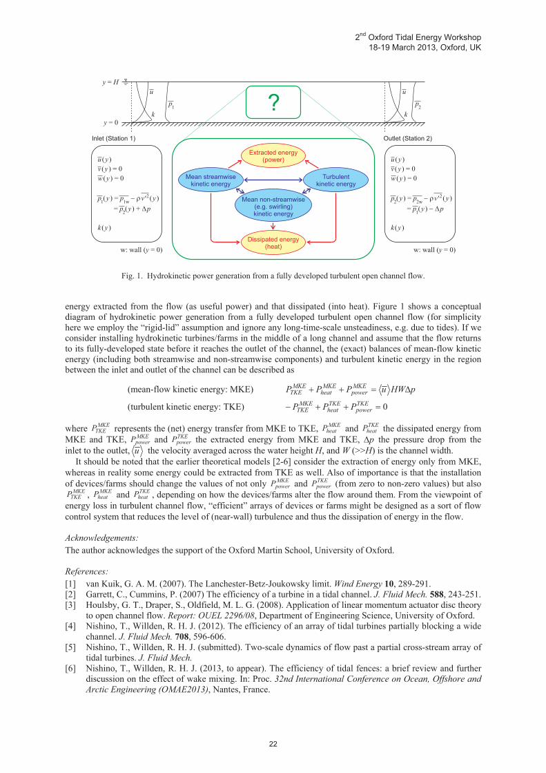
energy extracted from the flow (as useful power) and that dissipated (into heat). Figure 1 shows a conceptual diagram of hydrokinetic power generation from a fully developed turbulent open channel flow (for simplicity here we employ the “rigid-lid” assumption and ignore any long-time-scale unsteadiness, e.g. due to tides). If we consider installing hydrokinetic turbines/farms in the middle of a long channel and assume that the flow returns to its fully-developed state before it reaches the outlet of the channel, the (exact) balances of mean-flow kinetic energy (including both streamwise and non-streamwise components) and turbulent kinetic energy in the region between the inlet and outlet of the channel can be described as (mean-flow kinetic energy: MKE) pHWuPPP MKE

powerMKE

heatMKE

TKE

(turbulent kinetic energy: TKE) 0TKEpower

TKEheat

MKETKE PPP

where MKE

TKEP represents the (net) energy transfer from MKE to TKE, MKEheatP and TKE

heatP the dissipated energy from MKE and TKE, MKE

powerP and TKEpowerP the extracted energy from MKE and TKE, p the pressure drop from the

inlet to the outlet, u the velocity averaged across the water height H, and W (>>H) is the channel width. It should be noted that the earlier theoretical models [2-6] consider the extraction of energy only from MKE, whereas in reality some energy could be extracted from TKE as well. Also of importance is that the installation of devices/farms should change the values of not only MKE

powerP and TKEpowerP (from zero to non-zero values) but also

MKETKEP , MKE

heatP and TKEheatP , depending on how the devices/farms alter the flow around them. From the viewpoint of

energy loss in turbulent channel flow, “efficient” arrays of devices or farms might be designed as a sort of flow control system that reduces the level of (near-wall) turbulence and thus the dissipation of energy in the flow. Acknowledgements: The author acknowledges the support of the Oxford Martin School, University of Oxford. References: [1] van Kuik, G. A. M. (2007). The Lanchester-Betz-Joukowsky limit. Wind Energy 10, 289-291. [2] Garrett, C., Cummins, P. (2007) The efficiency of a turbine in a tidal channel. J. Fluid Mech. 588, 243-251. [3] Houlsby, G. T., Draper, S., Oldfield, M. L. G. (2008). Application of linear momentum actuator disc theory

to open channel flow. Report: OUEL 2296/08, Department of Engineering Science, University of Oxford. [4] Nishino, T., Willden, R. H. J. (2012). The efficiency of an array of tidal turbines partially blocking a wide

channel. J. Fluid Mech. 708, 596-606. [5] Nishino, T., Willden, R. H. J. (submitted). Two-scale dynamics of flow past a partial cross-stream array of

tidal turbines. J. Fluid Mech. [6] Nishino, T., Willden, R. H. J. (2013, to appear). The efficiency of tidal fences: a brief review and further

discussion on the effect of wake mixing. In: Proc. 32nd International Conference on Ocean, Offshore and Arctic Engineering (OMAE2013), Nantes, France.

Mean streamwisekinetic energy

Turbulentkinetic energy

Mean non-streamwise(e.g. swirling)kinetic energy

Extracted energy(power)

Dissipated energy(heat)

?

Inlet (Station 1) Outlet (Station 2)

u y

v y

w y

p y p v y

p y p

k y

( )

( ) = 0

( ) = 0

( ) = ( )

= ( ) +

( )

��

�1 1w

2

2'

u y

v y

w y

p y p v y

p y p

k y

( )

( ) = 0

( ) = 0

( ) = ( )

= ( )

( )

��

��2 2w

1

2'

y H=

y = 0

u

k

u

k

p2

p1

w: wall ( = 0)y w: wall ( = 0)y

Fig. 1. Hydrokinetic power generation from a fully developed turbulent open channel flow.

On the optimum place to locate a tidal fence in the Severn Estuary

Scott Draper*

Centre for Offshore Foundation Systems, University of Western Australia, Crawley, 6009, Australia

Summary: Much previous research has focused on tidal barrages in the Severn Estuary. In this paper we consider the alternative option of tidal stream devices (i.e. tidal turbines), and investigate the optimum place to locate a row of tidal devices in the Severn Estuary (in a fence) to generate power. Specifically, we find that this optimisation problem is more subtle than that for a barrage, with the best location dependent on the number of tidal devices installed within the fence. In particular, the optimum fence location is near the apex of the Estuary if few devices are used, but moves progressively West as the number of devices within the fence is increased.

Introduction and Methods Large tides in the Severn Estuary have attracted schemes for power generation for many decades. Most of these schemes have suggested the construction of a tidal barrage and, although they have been examined in detail (i.e. the ‘Bondi committee’ in 1981), have been turned down due to environmental and/or economic uncertainty.An alternative option to a barrage is to use tidal stream devices. These offer the relative advantages of allowing continuous water movement, sequential construction and placement below the water line. However, if turbines are used in the Severn Estuary an obvious question is where to place them. This question is considered herein. To simplify the problem we model the Severn Estuary as a channel with along channel coordinate x taking a value of zero 20 km upstream of Avonmouth (Fig. 1). We split the channel into three sections ( 1,2,3): (i) channel east of a tidal fence, (ii) channel immediately West of the fence, and (iii) channel further west where the width of the estuary changes abruptly (Fig. 1). In each section the channel is assumed to have linearly varying depth and width (i.e. , , with = 0.241 m/km adopted herein, and for sections (i) and (ii) 0.324 km/km). We also assume that the elevation and velocity are dominated by the M2 component, and ignore non-linearity’s in bed friction and energy extraction, so that the free surface elevation along the channel will take the form , where is the tidal frequency (2 /12.41 hrs), and the cross-sectional average velocity will be . The governing equations in each section of channel are then:

(1a,b)

where (taken herein to be 0.002) is a linearized bed friction parameter that is approximately equal to [2], where is a quadratic drag coefficient. Equation (1) has a general solution of the form:

(2)

where are Hankel functions of complex order and, and are complex coefficients. We solve for these six coefficients (2 in each section) subject to the following six boundary conditions:

(3a,b,c)(3d,e)(3f)

where , and are defined in Fig. 1 and the subscripts refer to the different sections of channel. The first two conditions (3a,b) ensure continuity of elevation and flow rate (with 1.7 the ratio in channel width either side of ). (3c) implies zero flow at the apex of the channel. (3d,e) define the (linearised) momentum sink of the tidal fence, in which = for devices of area , and is a thrust coefficient. We calculate this coefficient using actuator disc theory [3], ignoring the effect of Froude number. The power extracted by the fence, , and the power available to devices (net of mixing losses), , can then be given as

, (4a,b)


Section 1

Section 2

Section 3

x0

x1

x2x3

x [km]180 160 140 120 100

80 60

Fence

Fig. 1. Map of the Bristol Channel/Severn Estuary, including coordinate system adopted (adapted from [2]).

(2) (3)

Fig. 2. Maximum extractable power at different locations along the estuary. (solid line), from [2] (dashed line), for freely propagating wave (crosses). Fig.3 Solid lines are contours of available power (in GW). Thin lines are contours of

constant turbine area, with the area represented by each line increasing in the direction of the arrow. Note

where defines the flow through the turbines [3], and the overbar denotes average over the M2 cycle. The last condition in (3f) is the open ocean boundary condition, in which defines the impedance of the connecting sea/ocean, and and are natural elevation and velocity at the boundary . Several options are available to estimate , such as (i) a simple radiating wave independent of geometry west of the channel (similar to [1] or [4]), (ii) a value derived from a numerical model (as in [2]), or (iii) zero (representative of a clamped boundary).

Results and Conclusions Introducing a tidal fence at any given location along the channel, we find that there is a maximum amount of power, , that can be extracted as the turbine resistance is varied. Fig. 2 plots this maximum at all locations away from the apex of the channel. It is clear that the power extracted is dependent on the open ocean boundary condition, and that the best location in terms of extraction is to put the fence as far West as is practical (in agreement with [1] for a barrage). However, this is not generally the optimum place to locate a fence. This is because tidal devices are not perfectly efficient and produce a wake which dissipates energy through mixing. The losses due to this mixing reduce as turbines occupy a greater fraction of a channel cross-section, such that the fraction of extracted power available to tidal devices ( ) increases [3]. Consequently, if a fixed number of devices are installed in the Severn Estuary there is an interesting trade-off: moving the fence West leads to greater potential extraction (see Fig. 2), but moving the fence East will increase device blockage and efficiency due to the contracting channel geometry. This trade-off is played out graphically in Fig. 3. In this figure, for a given number of devices, a fence moves along the dashed contour lines. Clearly efficiency wins the trade-off, and the best tactic is to move the devices East so as to increase blockage and available power. This means that the optimum location is closer to the apex of the estuary when the number of devices (and turbine area) is small, and moves progressively west as the number of devices (and turbine area) increases. The optimum place to locate tidal devices in the Severn Estuary (to maximise available power) therefore depends on the number of devices. Of course it will also depend on many other factors, which are outside the scope of the present note.

S. Draper kindly acknowledges the support of the The Lloyd’s Register Foundation. References:[1] Rainey, R.C.T. (2009). The optimum position for a tidal power barrage in the Severn Estuary, J. Fluid

Mech. 636, 497-507.[2] Robinson, I. S. (1981). Tidal power from wedge-shaped estuaries – an analytical model with friction,

applied to the Bristol Channel, Geophys. J. R. astr. Soc. 65, 611-626.[3] Houlsby, G. T., Draper, S., Oldfield, M. L. G. (2008). Application of linear momentum actuator disc theory

to open channel flow. Report No. OUEL 2296/08, Department of Engineering Science, Univ. of Oxford.[4] Xia, J., Falconer, R.A. and Lin, B. (2010). Numerical model assessment of tidal stream energy resource sin

the Severn Estuary, UK, Proc. IMechE Part A: J. Power and Energy, 224, 969-983.

40 60 80 100 1200

2

4

6

8

Position from apex [km]

Ave

rage

Pow

er [G

W] 0.2

0.20.2

0.2

0.4

0.40.4

0.60.6

0.6

0.80.8

11

1.2 1.41.6

Blo

ckag

e, B

[-]

x [km]40 60 80 100 120

0.2

0.4

0.6

0.8


Tidal Stream Energy Assessment of the Anglesey Skerries

Sena Serhadlıoğlu*, Thomas A.A. Adcock, Guy T. Houlsby Department of Engineering Science, University of Oxford, OX1 3PJ, UK

Alistair G.L. Borthwick

Department of Civil and Environmental Engineering, University College Cork, Ireland

Summary: This paper analyses the available energy from tidal stream turbines at the Anglesey Skerries. Tidal turbines are represented by Linear Momentum Actuator Disk Theory [1]. The influence of extracting energy from the stream to the local hydrodynamics is modelled by implementing a line sink of momentum in a two-dimensional shallow water solver that uses a discontinuous Galerkin finite element method [2]. Results are presented using optimised turbine induction factor for different blockage ratios.

Introduction Two approaches have been applied to represent tidal turbines in a shallow water numerical model. Either the turbines can be represented as a discontinuity in the flow or the drag can be smeared over an area by enhancing the bed friction of a given node. Representing turbines as a discontinuity in the flow requires that the difference in water level across a tidal turbine to be known as a function of relevant parameters characterising the turbines and flow. This parameterisation of the tidal turbines is established by using LMADT. The equivalent upstream and downstream conditions are then imposed in the solution as a line sink of momentum [3].

Governing Equations and Numerical Method The ocean tides are modelled using the long wave equations, commonly known as the shallow water equations (SWEs). SWEs can be expressed as a time dependent, two-dimensional system of non-linear partial differential equations of hyperbolic type, which can be written in divergence form as [4],

∂u

∂t+ ∇ ⋅ F u( ) = s u( ). (1)

In the above equation u is vector of conserved variables, F is the flux vector, and s is the source (or sink) term vector. Equation 1 is discretised in space by using the discontinuous Galerkin (DG) finite element method and in time using SSP-Runge Kutta method. The DG formulation imposes the weak formulation of SWEs individually for each element, which enables to conserve mass locally and include discontinuities in the solution.

Representation of Tidal Devices LMADT enables us to have a relation between the upstream and downstream water depths across a turbine,

1

2

ΔH

H

⎛

⎝ ⎜

⎞

⎠ ⎟ 3

−3

2

ΔH

H

⎛

⎝ ⎜

⎞

⎠ ⎟ 2

+ 1+Fr2+CTBFr

2

2

⎛

⎝ ⎜ ⎜

⎞

⎠ ⎟ ⎟ ΔH

H−CTBFr

2

2= 0 , (2)

where, ΔH/H is the relative head difference, Fr is the upstream Froude number, CT is the thrust coefficient and B is the blockage ratio. This discontinuity in the water depth (as well as the horizontal velocity) can be modelled within the DG discretisation by modifying the numerical flux that is used to couple the elements.

Numerical Model In this paper, we are presenting a parametric study of the power availability around the Anglesey Skerries. A two-dimensional unstructured finite element model of the southwest of UK coasts has been created, which has been forced with the most significant tidal constitutes of M2 and S2. The model has been validated against field data. Focusing around the Anglesey Skerries, four rows of turbine arrays that extend to 9 km have been placed approximately 300 m offshore of the Skerries in parallel to each other. This paper considers 3 different array locations and an example of installing arrays in parallel and series. The array configuration ASA1 refers to a row



of turbines that extend to 4.5 km located on the offshore of the Skerries, whereas ASA2 is situated closer to the Skerries. ASB2 row is 1 km NE of and lies parallel to ASA2 array.

Results The parametric studies are based on investigating the effect of: a) location, b) connectivity of arrays (serial/parallel), c) blockage ratios, and d) turbine induction factors, on the power availability. Table 1 gives a summary of maximum available power, turbine efficiency for several turbine array locations and configurations. Herein, we are also showing the economical gain, which corresponds to the ratio of energy gain by connecting turbine arrays in parallel or in series. Figure 1 shows a) the raw power generated for a spring/neap tide for the most favourable array configuration and, b) the power availability for a spring tide regarding the M2 tidal constituent. Table 1. Summary of available power, and economical gain factors for several configurations.

Available Power (MW) Economical Gain Configuration B=0.5 B=0.3 B=0.1 B=0.5 B=0.3 B=0.1

ASA1 124.3 54.7 12.7 - - - ASA2 145.3 70 17.2 - - -ASB1 139.8 67.3 16.6 - - -

ASA1+ASA2 301.2 130.8 30.2 1.117 1.049 1.01 ASA2+ASB2 199.1 114.6 32.4 0.698 0.835 0.959

Conclusions In the analysis, it is observed that placing the turbine array closer to the Skerries results in higher power generation than placing them further offshore. Regarding the configuration of the arrays, it is seen that placing the arrays in parallels is economically more effective than as in series. This improvement diminishes with smaller blockage ratios. In serial configurations, the energy loss with respect to the wake mixing lessens by decreased blockage effect. Acknowledgements: This work was funded and commissioned by the Energy Technologies Institute as part of the PerAWaT project. The authors would like to thank the Oxford Supercomputing Center for allowing us to use their computing resources. References: [1] Houlsby, G. T., Draper, S., Oldfield, M. L. G. (2008). Application of linear momentum actuator disc theory to open

channel flow. Report No. OUEL 2296/08, Department of Engineering Science, University of Oxford. [2] Draper, S. (2011). Some analytical and numerical studies of tidal stream energy extraction in coastal basins. DPhil

thesis, University of Oxford. [3] Draper, S., Borthwick, A.G.L., and Houlsby, G.T. (2011). Energy potential of a tidal fence deployed near a coastal

headland. EWTEC 2011, Southampton, UK. [4] Toro, E. F. (2001). Shock-capturing methods for free-surface shallow flows, Wiley, New York.

Fig. 1. Power availability for ASA1+ASA2 array configuration. (a) Raw available power for B = 0.5 in a highly blocked

case, (b) Available power for a spring tide for M2 tide.


Influence of tidal energy extraction on fine sediment dynamics

Peter E. Robins Centre for Applied Marine Sciences, Bangor University, LL59 5AB, UK

Summary: Tidal energy extraction and fine sediment dynamics are simulated at a high-velocity location off the north-west coast of Anglesey, Wales (UK). This site generates some of the largest tidal velocities in the Irish Sea (> 2.5 m s-1, during spring tidal flow), due to high tidal amplitudes and flow being constricted by a collection of small rocky islands known as The Skerries. This site has been highlighted as one of seven specific regions of interest around the UK for ‘first generation’ tidal energy extraction and has been leased by the Crown Estate for commercial development [1].

Introduction

The affect that tidal energy extraction might have on suspended sediment concentrations is investigated in the Skerries channel, Wales, UK, where a turbidity maximum is persistent throughout the year [2]. Turbidity maxima occur in regions of strong tidal energy dissipation where there are high concentrations of suspended sediments, detritus, zooplankton and fish early-life stages. These areas enhance secondary production, and serve as critical nursery areas for economically important species [3]. The Anglesey Turbidity Maximum (ATM) was simulated [2] using a two-dimensional aggregation/disaggregation model, with two different sediment size classes, and maintained by the disaggregation of suspended flocs (~140 m) into smaller particles (~70 m). High suspended sediment concentrations (13 mg l-1) were simulated during winter, with seasonal variability of the order 7 mg l-1, which was comparable to visible-band satellite observations [4].

Methods

A finite-element morphodynamic model (TELEMAC Modelling System [5]) was applied at Irish Sea scale. The suspended and bedload sediment transport module (SISYPHE) is internally coupled with the hydrodynamics (TELEMAC-2D), using the Bijker’s transport formula [6]. While this condition is not accurate for the whole of the Irish Sea (e.g. some areas contain bed rock or cobbles only), the Bijker transport formula is appropriate around Anglesey. The model mesh gives fine resolution (< 250 m) around Anglesey and coarser resolution elsewhere, and mapped onto digitized bathymetry data (250 m resolution). Simulated velocities (RUN-1) were well validated against coastal tide-gauge measurements and suspended sediment concentrations collected off north-west Anglesey during May 2012, revealing the dominant size class to be 85 m (Fig. 1). In order to simulate the ATM, a novel approach was designed whereby a maximum erodable bed depth of 2 m was enforced throughout the domain, ensuring a finite Irish Sea sediment supply, as occurs naturally [2]. Consequently, if the model bed erodes by 2 m, no further erosion takes place; similar in effect to flow over bed rock, yet sediments can still flow here in suspension, as was the case through the Skerries. Tidal energy extraction from multiple turbines is implemented in the model by inducing a drag force, F, on the flow at the point of energy extraction [7]; F=0.5*( CDAU), where (kg m-3) is the seawater density and A (m2) is the effective area of the turbine on which the undisturbed velocity U (m s-1) acts. The drag coefficient, CD, increases the blockage effect on the flow, which in turn decreases the local velocity. As the drag coefficient increases, the extracted power (in Watts) by each turbine increases, and can be calculated using: P=FU.

Results Two additional scenarios were modelled to incorporate tidal energy extraction with ‘medium-scale’ (~10 MW) extraction from a site in the Skerries (RUN-2) and ‘large-scale’ (~20 MW) tidal energy extraction from the same site (RUN-3). Peak spring velocities were reduced by 10-15% for RUN-2 and by 15-20% for RUN-3, at the point of energy extraction (Fig 2c). Further upstream, effects of energy extraction were less (Fig. 2b,d), being negligible 4 km away (Fig. 2a,e). In consequence, suspended sediment concentrations were reduced slightly (by 5-10%) at the point of energy extraction (Fig. 2h), again decreasing further afield (Figs. 2f,g,i,j).


Conclusions

Modelled suspended sediment concentrations in the region of the Anglesey Turbidity Maximum correspond with observations (in the range 0-20 mg l-1). Moreover, modelled suspended sediment concentrations are maintained throughout a lunar cycle; a process that some other models have found difficult to reproduce [8]. We have achieved this by imposing a non-erodable bed after some initial scour, thereby ensuring a finite volume of source material into and out of the ATM, without unrealistic erosion at the ATM, which mainly comprises cobbles and bed rock [2]. ‘First generation’ energy extraction (of the order 10-20 MW) will reduce velocities and suspended sediment concentrations locally; however these changes are an order of magnitude less than seasonal variability predicted [2] and, therefore, considered negligible. Consequently, this is a positive result for the marine energy industry, and also for the ecological implications this may have. References:

[1] Iyer, A.S., Couch, S.J., Harrison, G.P., Wallace, A.R. 2013. Variability and phasing of tidal current energy

around the United Kingdom. Renewable Energy 51: 343-357. [2] Ellis, K., Binding, C., Bowers, D.G., Jones, S.E., Simpson, J.H. 2008. A model of turbidity maintenance in

the Irish Sea. Estuarine, Coastal and Shelf Science 76: 765-774. [3] Bowers, D., Gaffney, S., White, M., Bowyer, P. 2002. Turbidity in the southern Irish Sea. Continental Shelf

Research 22: 2115-2126. [4] Bowers, D., Ellis, K., Jones, S.E. 2005. Isolated turbidity maxima in shelf seas. Continental Shelf Research

25: 1071-1080. [5] Hervouet, J.M. 2007. Hydrodynamics of Free Surface Flows. 1st Edition, John Wiley and sons, Press 2007. [6] Bijker, E.W. 1992. Mechanics of sediment transport by the combination of waves and current. In:

Proceedings of the 23rd International Conference on Coastal Engineering. ASCE, Venice, Italy, pp. 147–173. [7] Lalander, E., M. Leijon. 2009. Numerical modelling of a river site for in-stream energy converters. Proc. 8th

European Wave and Tidal Energy Conf., Sweden. [8] Aldridge, J.N., Kershaw, P., Brown, J., McCubbin, D., Leonard, J.S., Young, E.F. 2003. Transport of

plutonium (239/240Pu) and caesium (137Cs) in the Irish Sea: Comparison between observations and results from sediment and contaminant transport modelling. Continental Shelf Research 32: 869-899.

Figure 1. TELEMAC Irish Sea model output, showing (a) peak spring depth-averaged suspended sediment transport (m3 s-1 m-1). The boxed area off north-west Anglesey is enlarged in (b), showing the position of the Skerries channel and the formation of the Anglesey Turbidity Maximum (ATM). Modelled volume concentrations of suspended sediment ( l l-1) (red curve) during May 2012 at a point outside the Skerries, marked ‘x’ in (b), are shown in (c), compared with LISST data.

Figure 2. Impact of tidal energy extraction on depth-averaged velocities (a-e) and suspended sediment volume concentrations (f-j), in the Skerries channel. Time series are shown at the point of energy extraction and also upstream and downstream of the TEC array. Three scenarios have been modelled: no energy extraction (solid lines), a ‘medium-scale’ (~10 MW) TEC array (dashed lines), and a ‘large-scale’ (~20 MW) TEC array (dotted lines).


On the performance of axially aligned tidal stream turbines using a Blade Element Disk approach

Ian Masters, Alison J. Williams, T. Nick Croft, Rami Malki College of Engineering, Swansea University, SA2 8PP, UK

Summary: Turnock et. al. [1] have published a CFD analysis of a single tidal stream rotor and propose an empirical model of the performance of multiple rotors arranged directly behind each other. The rotors downstream are assumed to have cumulative effects from the rotors upstream. The approach used in this work is a combined Blade Element Momentum Theory Computational Fluid Dynamics model, which allows a good approximation of the hydrofoil physics at the rotor with reasonable computational cost. The Turnock proposal is tested using the BEM-CFD model and it appears that cumulative effects are less than expected.

Introduction The performance of tidal stream arrays is of great interest to the industry. However, in the absence of full

scale data, predictions are made using tank testing, CFD models and empirical corrections. Turnock et al. [1] suggested that for a series of turbines aligned linearly along the flow direction, the power output of any given turbine within the arrangement can be determined by applying a common factor to the power output of the turbine immediately upstream. However, Turnock only conducted simulations for a single rotor and made these conclusions based on observations of flow velocity recovery. This hypothesis is tested here by conducting simulations of four rotors with a longitudinal spacing of 10 and 20 diameters. From earlier work [2] we know that wake recovery is related in inlet velocity. A number of studies have also shown some evidence for increased mixing and shorter wakes as turbulence increases.

Methods The method is described in [3] and can be summarised as follows. The Navier-Stokes equations, representing the conservation of mass and momentum are solved:

=0

where ρ is the density, ui is the i’th component of the velocity vector, p is pressure, μlam and μt are the dynamic laminar and turbulent viscosities respectively, and Si includes additional sources due to the moving rotor as follows:

d d

d d

The turbine rotor source is represented in the model according to the principles of Blade Element Momentum Theory. The blades are discretised into thin elements of width dr, and the forces exerted by each element on to the oncoming fluid are determined. Tabulated data characterising the blade geometry (chord length, c and twist angles) and hydrodynamic properties (lift and drag coefficients, and with angle of attack) are required for the calculations. The local velocity, and flow inclination angle, ,

depend on uθ , uz and Ω, the tangential, axial and angular velocities respectively.

Results Velocity contours for a longitudinal spacing of 10 and 20 diameters are shown in Figure 1 and corresponding power outputs in Figure 2. Velocity profiles along the centreline for the two spacing conditions given in Figure 3 clearly show a velocity drop across each device.

Conclusions The trends observed diverge from suggestions made by Turnock. In both cases, there is a levelling off at around 20 diameters downstream of the first turbine beyond which power outputs are virtually equal for consecutive devices. The modelling has been conducted in a uniform channel and preliminary models [4] show that water surface gradient may also affect wake lengths. Obviously, the methodology should be verified against measured data in real sea conditions.


Acknowledgements:

References: [1] Turnock, S.R., Phillips, A.B., Banks, Joe and Nicholls-Lee, R.F. (2011) Modelling tidal current turbine

wakes using a coupled RANS-BEMT approach as a tool for analysing power capture of arrays of turbines. Ocean Engineering, 38, (11-12), 1300-1307. (doi:10.1016/j.oceaneng.2011.05.018).

[2] Malki, R. , Masters, I., Williams, A.J., Croft, T.N., (2011) The variation in wake structure of a tidal stream turbine with flow velocity, 4th Int. Conf. Computational Methods Marine Eng., MARINE 2011, 426-437

[3] Malki, R., Williams, A.J., Croft, T.N., Togneri, M. and Masters, I. (2013) A Coupled Blade Element Momentum - Computational Fluid Dynamics Model for Evaluating Tidal Stream Turbine Performance. Applied Mathematical Modelling, 37 (5), 3006–3020, (doi: 10.1016/j.apm.2012.07.025)

[4] Malki, R., Masters, I., Williams, A.J., Croft, T.N., (2012) A numerical investigation into tidal stream turbine wake dynamics and device performance in non-uniform flows, Proc. 22nd Int. Offshore Polar Eng. Conf., ISOPE 2012, Pages 745-750

Figure 1: Velocity contours around four rotors aligned axially. 10 diameters spacing (top) and 20 diameters spacing (bottom).

Figure 2: The effects of wakes on the downstream

turbine power output in a 4 turbine array. Blue diamonds are 10 diameter spacing, Red squares 20 diameter spacing

Figure 3: Centreline velocity profile with the second

rotor at the zero position

Characterisation of the near-wake of a Horizontal Axis Tidal Stream Turbine in Non-uniform steady flow

Siân C. Tedds1, Tiago A. de Jesus Henriques, Robert J. Poole School of Engineering, University of Liverpool, UK

Ieuan Owen School of Engineering, University of Lincoln, UK

Summary: This paper details an experimental study which has characterised the near-wake of a model Horizontal Axis Tidal Stream Turbine (diameter = 0.5m) in a large-scale recirculating water channel facility. A “flow-profiler” has been designed and placed upstream of the turbine, producing a1/5th power-law velocity profile through the depth of the channel. The thrust and power coefficients of the turbine have been characterised and compared to uniform flow. An Acoustic Doppler Velocimeter is used to proved detailed three-dimensional mean and turbulent flow field information at five different depths across the full width of the channel downstream of turbine.

Introduction As well as characterising the power output for a tidal stream turbine it is also important to characterise the wake of a turbine. For example, as turbines are likely to be placed in farms or arrays to make them commercially viable, wake recovery length is crucial for the appropriate spacing between turbines. Also, knowledge of the wake is important so that effects on the sea bed can be investigated. Previous experimental studies have been confined to measure the wake effects with upstream uniform flow (e.g. [1], [2]). This study investigates the near-wake downstream of a turbine in a non-uniform steady flow at five different heights across the width of the channel.

Experimental MethodsA three-bladed Horizontal Axis Tidal Stream Turbine with a diameter of 0.5m, was assembled with optimum blade pitch angle (6o for maximum power output [3]). The turbine was tested in the University of Liverpool high-speed water flume, which has a working section of 1.4m wide, 3.7m long and 0.8m deep, with an inlet velocity set such that Reynolds number effects are negligible and the model results are representative of the full scale. The turbine and the flow field in its wake has been well characterised in uniform flow with a low turbulence intensity (approximately 2%) [3]. A non-uniform “flow-profiler”, comprising a series of 15mm horizontal bars set varying distances apart, was placed at the inlet to the flume working section to produce a vertical velocity profile represented by a 1/5th power-law, and with an integral average upstream velocity of 0.82m/s and an average turbulence intensity of approximately 5%. The three-dimensional velocities and turbulence statistics of the flow produced by the “flow-profiler” were characterised using an Acoustic Doppler Velocimeter ((ADV) Nortek Vectrino+) with a sample frequency of 200Hz and 10,000 samples collected at each measurement location to ensure a 99% confidence interval.

During the experimental tests the turbine was located at a depth of 0.4m, 1m downstream of the ``flow-profiler'', giving a blockage ratio of approximately 16%. The output power and the thrust on the turbine were measured in both the uniform and non-uniform flows and compared. The near-wake measurements were made using the ADV, taken at downstream distances between 1.5 and 5 turbine diameters with a series of spanwise profiles and at various depths to fully map the flow field in the near-wake. The maximum distance between each measurement location in the spanwise profiles was 50mm, thereby providing a comprehensive data set. The near-wake velocity components in non-uniform flow have been compared with those in uniform flow.

Results When plotted non-dimensionally, using the integral average upstream velocity, the output power and thrust in both the uniform and non-uniform flow are seen in figure 1(a) and (b) to approximately collapse onto a single characteristic curve, confirming CFD results by Mason-Jones et al. [4].

Figure 2 shows the maximum streamwise velocity deficit downstream of the turbine in uniform and non-uniform flow. At a depth equal to the centreline of the turbine, the three-dimensional velocities and turbulence statistics downstream of the turbine for the non-uniform flow is quantitatively the same as that with the uniform flow. At 1 Corresponding author. Email address: [email protected]

the depths above the centreline, where the upstream flow is faster, the recovery of the streamwise velocity downstream of the turbine is slower than with uniform flow. Conversely at depths below the centreline the streamwise velocity recovers more quickly in the non-uniform flow compared with the uniform flow. These variations of the downstream flow field are a result of the non-uniform inlet profile being propagated into the near-wake of the turbine. The effects of the swirl from the turbine blades are more prominent in the non-uniform flow, and this can be seen in both the transverse and spanwise velocity components downstream of the turbine at all the considered depths. Figure 3 shows the maximum turbulent kinetic energy (TKE) downstream of the turbine at a depth of the centre of the turbine, it can be seen that the maximum TKE decays at a similar rate for both flow conditions.

Conclusions The upstream flow has minimal effect on the average power and thrust coefficients. However the upstream flow has a considerable effect on the near-wake downstream of a turbine. The results show that even for turbines with identical mean thrust coefficients the near-wake characteristics can be significantly modified by the upstream flow. References: [1] Maganga, F., Germain, G., King, J., Pinon, G., Rivoalen, E. (2010). Experimental chraracterisation of flow effects on

marine current turbine behaviour and on its wake properties. IET Renewable Power Generation 5, 498-509. [2] Stallard, T., Collings, R., Feng, T., Whelan, J. (2013). Interactions Between Tidal Turbine Wakes: Experimental Study

of a Group of 3-Bladed Rotors. Philosophical Transactions of The Royal Society. 371, 20120159. [3] Tedds, S.C., Poole, R.J., Owen, I., Najafian, G., Bode, S.P., Mason-Jones, A., Morris, C., O’Doherty, D.M.,

O’Doherty, T. (2011). Experimental Investigation Of Horizontal Axis Tidal Stream Turbines. In: Ninth European Wave and Tidal Energy Conference, Southampton, UK.

[4] Mason-Jones, A., O’Doherty, D.M., Morris, C.E., O’Doherty, T., Byrne, C.B., Prickett, P.W., Grosvenor, R.I., Owen, I., Tedds, S.C., Poole, R.J. (2012). Non-dimensional scaling of tidal stream turbines. Energy. 44, 820-829.

(a)

Figure 1: Power and thrust coefficients of the turbine in uniform and non-uniform steady flows.

(b)

Figure 2: Streamwise velocity deficit downstream of the turbine at a height equal to the centre of the turbine in uniform and non-uniform steady flows.

Figure 3: Normalised maximum TKE downstream of the turbine at a height equal to the centre of the turbinein uniform and non-uniform steady flows.

2nd Oxford Tidal Workshop

18 - 19 March 2012, Oxford ,UK

Tidal Turbine Wake Recovery due to Turbulent Flow and Opposing Waves

Alex Olczak*, Tim Stallard and Peter Stansby,School of Mechanical Aerospace and Civil Engineering,University of Manchester, M13 9PL

Summary: Detailed measurements are presented showing the modification of wake recovery of a single tidal stream

turbine subjected to opposing waves of varying frequency and height. Waves of frequency 0.5 to 0.8 Hz and increasing

heights are considered representing full-scale waves of 10-16 s over a flow of 3.7 m/s in 31 m depth. Vertical velocity

deficit profiles within the wake differ considerably with wave frequency; waves of 0.5Hz and 0.6Hz reduced the velocity

deficit in the lower half of the water column whilst 0.7Hz and 0.8Hz waves caused a reduced deficit in the upper half.

Further analysis of the far wake recovery is presented for two wave conditions with similar wave energy. The regions

over which the far wake recovery is enhanced by opposing waves is similar to that for the near wake. Analysis of

ambient flow indicates the enhanced wake recovery caused by the waves may occur because of the greater ambient

flow fluctuations of the combined wave current flow.

BackgroundFlow velocities of U>1.5 m/s are typically considered suitable for electricity generation by horizontal axis turbines.

Many of the sites where these flow speeds occur are at exposed locations where waves and currents coexist. The area

available for the deployment of turbines is often limited by the local topography of these sites. To maximise the energy

extraction from sites with suitable flow velocities devices are likely to be installed in arrays. The lateral spacing of

turbines will be somewhat device dependant however the stream-wise spacing will be governed by the rate of wake

recovery. The rate of wake recovery will therefore effect both the number of turbines located at a site and subsequently

the power output of an array. Recent experiments have measured the flow field downstream of a single turbine operating

in a shallow turbulent flow. The rotors momentum extraction is commonly replicated by the use of scaled turbines [1]

or porous disks [2] where the disk porosity is such that the force exerted on the fluid by the disk is equivalent to that of

a rotor. However to-date the effect of combined wave current flow on wake recovery flow has received little attention.

MethodologyA shallow turbulent flow with a depth averaged stream-wise velocity (U∞) of 0.46 m/s is developed in a flume with

water depth (d) = 0.45m and width (W)= 11d. Applying Froude scaling at 1:70 geometric scale this is representative of

a tidal flow with U = 3.7m/s and d = 31m. Inflow velocity profiles were recorded at the flume centre for a range of wave

heights. The addition of opposing waves leads to an increase in velocity fluctuations, apparent as increased turbulence

intensity, for all wave conditions with depth profile of fluctuations dependent on wave frequency. A 3 blade rotor of

diameter (D) = 0.67d is used to represent both momentum extraction and wake rotation. The rotor foil was chosen such

that in steady flow the Ct(λ) is similar to a generic full scale turbine [3]. The axial force is recorded from a strain gauge

located above the water line. During experiments a motor is used to apply constant torque so that the rotor is operating

with a mean tip speed ratio (λ) of 5.5± 5% resulting in a mean thrust coefficient CT = 0.90. The wave kinematics

are such that the amplitude of velocity fluctuations at hub height is between 18-36% of mean velocity. This variation

in inflow velocity causes a large periodic variation in time varying rotor thrust compared with a rotor operating in

steady flow. Depth profiles of time varying velocities u(t),v(t) and w(t) within the wake were recorded using a Nortek

Acoustic Doppler Velocimeter (ADV) which is accurately positioned within the flow by computer controlled traversing

equipment. Velocities are recorded using a sample frequency of 200Hz and a duration of 1min.

*Alex Olczak

[email protected]

2nd Oxford Tidal Workshop

18 - 19 March 2012, Oxford ,UK

0 0.2 0.4 0.6 0.80

0.2

0.4

0.6

0.8

1

Udef

z/d

(a) 2D -Udef

0 20 40TI

x(%)

(b) 2D - TIx

0 0.2 0.4 0.6 0.80

0.2

0.4

0.6

0.8

1

Udef

z/d

(c) 4D - Udef

0 20 40TI

x(%)

(d) 4D - TIx

Figure 1: Velocity Deficit and Turbulence Intensity at 2D and 4D downstream. [No Wave (x), 0.5Hz Wave III (Hm0 =90.2mm) (O) and 0.8HZ Wave I (Hm0 = 85.9mm))(�)]

Conclusions and DiscussionAnalysis of time varying CT during tests showed a large variation compared to a rotor operating in steady flow.

However mean CT for each wave conditions was similar to that for steady flow and therefore wake generation was con-

sidered similar. Depth profiles of velocity deficit and turbulence intensity in the near wake (2D and 4D) are presented

for each wave condition. A reduction in wake deficit and therefore enhanced wake recovery is shown to occur over part

of the wake for each wave condition considered. The region of the wake over which the enhanced recovery is observed

is dependant on the wave frequency, as expected higher energy waves are shown to cause more recovery than smaller

waves. Wake recovery may be related to the turbulence intensity of the ambient flow and so the increased rate of wake

recovery is expected to to be related to the wave induced kinematics. Two wave conditions are selected with similar

mean energy density. Far wake recovery over the range 2D < X < 12D for these two conditions show a similar trend

with the 0.8Hz wave predominately affecting the upper wake and the 0.5Hz wave enhancing wake recovery throughout

the depth.

References[1] F. Maganga, G. Germain, J. King, G. Pinon, and E. Rivoalen, “Experimental characterisation of flow effects on

marine current turbine behaviour and on its wake properties,” IET Renewable Power Generation, vol. 4, no. 6, p.

498, 2010.

[2] A. S. Bahaj, L. Myers, M. Thomson, and N. Jorge, “Characterising the wake of horizontal axis marine current

turbines,” in 7th European Wave and Tidal Energy Conference, Porto, Portugal, 2007.

[3] J. I. Whelan and T. Stallard, “Arguments for modifying the geometry of a scale model rotor,” in 9th EuropeanWave and Tidal Energy Conference (EWTEC), Porto, Portugal, 2012.

*Alex Olczak

[email protected]

2nd Oxford Tidal Energy Workshop


Individual Based Modelling Techniques and Marine Energy

Thomas Lake∗, Ian Masters and T. Nick Croft

College of Engineering, Swansea University, Singleton Park

Summary: The development and deployment of marine energy devices places a number of requirements on develop-

ers to investigate the impact of the device and associated maintenance and installation activity on the environment.

This impact includes effects of this activity on other existing marine users, and also the effect on any marine mammal

population. Individual Based Modelling (IBM) techniques coupled with sufficient information about the behaviour

of a species may provide a way to investigate these responses. These techniques require sufficient background in-

formation to develop a simulation accounting for the likely influences on a species. This discussion will look at the

requirements of this sort of simulation, both computationally and in terms of input data.

Individual Based Modelling MethodsIndividual Based Models (IBMs) are a form of computer model that simulates interactions between a population

of entities and/or their surrounding environment. These entities are sometimes referred to as ‘agents’ or ‘boids’[1],

and the latter term will be used here. Boids are given a set of rules that are used to determine how that boid

will behave within the simulation. The number and detail of these rules varies depending on the simulation, but

even a very simple set of rules can lead to behaviour that "corresponds to the observer’s intuitive notion" of a

behaviour[1]. In that example, 3 simple rules gave rise to plausible looking flocks of birds for a computer animation.

For the purposes of simulating specific species in a specific environment, a more detailed set of rules is likely to be

required.

The decisions made by each boid typically include movement [1, 2, 3]. The rules concerning movement may treat

the boids as point particles with orientation[1], or as mechanical entities that move in a more realistic fashion[2].

In addition to movement, the rules may decide on mental states or ‘intentions’[2] which can be used to decide how

the boid reacts to a given scenario.A ‘panicked’ creature may flee when it detects another boid nearby, but may wait

until the boid is closer in another state. These states could also be exposed to the other boids within the simulation.

A further variation is the addition of a memory to the boids, so that each is able to remember where it has been and

the conditions of that area at the time it left[3]. This can be combined with simulated resource availability, with

the domain split into patches and resources in each patch being increased or depleted by the boids. This allows the

environment to be affected by the boids.

Field and Background DataAny attempt to predict the behaviour of marine life in the vicinity of turbines would be meaningless without

sufficient understanding of their existing behaviour. It is also necessary to gain an understanding of how these

behaviours relate to the environmental conditions around them.

Obtaining data to reach this understanding is a challenge for any sort of animal behaviour research, but is a

particular issue when considering animals in the marine environment. Observational data may be limited by sea

states and prevailing weather conditions, and may not be able to capture the underwater behaviour of diving and

swimming animals. The environment itself also adds additional variables to be considered - varying speeds and

heights of water due to the tide, variation in that tidal cycle across spring and neap tides and so on - in addition

to most of the variables that apply to land based models. Electronic tagging of animals allows the movement of

individuals to be tracked and analysed. These tags can transmit data via satellites, radio or GSM, or log data to be

read when the tag is collected[4].

Physiological data regarding fish and smaller marine animals may be useful to determine the risk to these crea-

tures due to a marine energy device[5]. This may be useful to incorporate into an IBM where fish are the main

∗Corresponding Author

Email: [email protected]

focus, or are included as prey for larger marine life. This data can be difficult to obtain for larger and/or protected

species, but there has been a study of turbine blade impacts on adult killer whales[6], which examined how they

might be injured if it were to be struck by a tidal stream turbine blade.

The influences selected for use in an IBM are also dependent on the available data, in a marine environment this

data will almost certainly include flow data and bathymetry[7]. The flow data might be derived from measurements,

or taken from the results of a Computational Fluid Dynamics (CFD) model. These results can be compared to

measured velocities, obtained using acoustic Doppler current profiler (ADCP) techniques or similar[8]. Underwater

noise is another potential contribution to animal behaviour in a marine environment which may be altered by the

installation and operation of marine energy devices. Noise due to turbulence and water flow is exacerbated in fast

flowing currents, such as those where marine energy devices may be installed. Other sources of noise include boats

and other marine users, turbulence and noises emitted by other marine animals[8, 9].

Parallelism and Implementation of Individual Based ModelsManaging the computational cost of large populations is an important consideration in IBMs, particularly if

the rules used are particularly complex or refer to many sources of information. It is possible to decrease the time

required to run a simulation by distributing the computations across multiple processors/nodes. Every boid needs

to run through it’s decision making procedure, examining any required information. If the boids interact with each

other, even if only in terms of movement decisions, this also requires searching the list of all boids in the simulation

to determine which are nearby. This cost can be reduced by partitioning the data and shrinking the size of the

population searched by each boid[10].

Related to this is the difficulty of incorporating the different data sets efficiently, which requires taking into

account the types of grid and resolution of the data, as well as how this data fits with the partitioning used. If the

simulated environment has been split into patches or areas with properties associated with them to represent boid

driven changes to the environment then these areas may add an additional constraint to the partitioning process.

References[1] C. W. Reynolds, “Flocks, herds and schools: A distributed behavioral model,” ACM SIGGRAPH Computer Graphics,

vol. 21, no. 4, pp. 25–34, 1987.

[2] X. Tu and D. Terzopoulos, “Artificial fishes: Physics, locomotion, perception, behavior,” in Proceedings of the 21st annualconference on Computer graphics and interactive techniques, pp. 43–50, ACM, 1994.

[3] H. Saarenmaa, N. D. Stone, L. Folse, J. Packard, W. Grant, M. Makela, and R. Coulsen, “An artificial-intelligence modelingapproach to simulating animal habitat interactions,” Ecological Modelling, vol. 44, pp. 125–141, 1988.

[4] D. Thompson, “Assessment of Risk to Marine Mammals from Underwater Marine Renewable Devices in Welshwaters (on behalf of the Welsh Government), Phase 2: Studies of Marine Mammals in Welsh High TidalWaters, Annex 1 Movements and Diving Behaviour of Juvenile Grey Seals in Areas of High Tidal Energy.”http://www.marineenergypembrokeshire.co.uk/publications-resources, July 2012. JER3688.

[5] M. R. Willis, M. Broudic, C. Haywood, I. Masters, and S. Thomas, “Measuring underwater background noise in high tidalflow environments,” Renewable Energy, vol. 49, pp. 255–258, January 2013.

[6] T. Carlson, B. Watson, J. Elster, A. Copping, M. Jones, M. Watkins, R. Jepsen, and K. Metzinger, “Assessment of strike ofadult killer whales by an openhydro tidal turbine blade,” Tech. Rep. PNNL-22041, Pacific Northwest National Laboratory,November 2012.

[7] T. O’Doherty, A. Mason-Jones, D. OâĂŹDoherty, P. Evans, C. Wooldridge, and I. Fryett, “Considerations of a horizontalaxis tidal turbine,” in Proceedings of the Institution of Civil Engineers - Energy, vol. 163, pp. 119–130, 2010.

[8] M. R. Willis, I. Masters, S. Thomas, R. Gallie, J. Loman, A. Cook, R. Ahmadian, R. Falconer, B. Lin, G. Gao, M. Cross,N. Croft, A. J. Williams, M. Muhasilovic, I. Horsfall, R. Fidler, C. Wooldridge, I. Fryett, P. Evans, T. O’Doherty,D. O’Doherty, and A. Mason-Jones, “Tidal turbine deployment in the bristol channel: a case study,” in Proceedings of theInstitution of Civil Engineers - Energy, vol. 163, pp. 93–105, August 2010.

[9] M. Broudic, T. Croft, M. R. Willis, I. Masters, and S.-H. Cheong, “Comparison of underwater background noise duringspring and neap tide in a high tidal current site: Ramsey sound,” in Proceedings of the 11th European Conference onUnderwater Acoustics, July 2012.

[10] B. Zhou and S. Zhou, “Parallel simulation of group behaviors,” in Proceedings of the 2004 Winter Simulation ConferenceR. G. Ingalls, M. D. Rossetti, J. S. Smith, and B. A. Peters, eds., 2004.

Numerical Modelling of a Laboratory Scale Tidal Turbine

Robert M. Stringer*, Jun Zang Department of Architecture & Civil Engineering, University of Bath, BA2 7AY, UK

Andrew J. HillisDepartment of Mechanical Engineering, University of Bath, BA2 7AY, UK

Summary: Computational Fluid Dynamics (CFD) has been used to model a cross-flow type tidal turbine that has undergone testing at laboratory scale. The turbine, a three-bladed transverse design, was built and tested by the University of Oxford as a prototype in the development of the THAWT device [1]. To achieve an accurate representation of the experimental data, issues surrounding scale, suitability of solvers and accurate replication of the test, are considered in the development of a numerical model. Using a logical validation procedure throughout, the final model achieves a high degree of correlation with the experimental values. Finally, the model is expanded to explore scaling, flow phenomena, and alternative inflow conditions.

Introduction Cross-flow turbines are currently under investigation by a number of academic and industrial projects

throughout the world. They offer a number of advantages over conventional axial designs, such as swept area, scalability and blockage [2]. The design investigated is a cross-flow turbine in its simplest form, a three-bladed device with circular endplates. Fig. 1 provides an illustration of the cross-flow concept; resolving rotation velocity (Utan) and free stream velocity (U ), an effective velocity (Ueff) is obtained, the resulting lift (L) provides a driving torque to the system. The efficiency of a fixed pitch device in uniform flow is primarily determined by the Tip Speed Ratio (TSR) or = Utan/U , too slow and excessive stall occurs, too fast and angle of attack (α) becomes insufficient to induce useful lift. This relationship is plotted in Fig. 2 for three TSRs.

Fig. 1. Cross-section of a cross-flow tidal turbine Fig. 2. Graph of angle of attack with rotation position

In order to examine the efficiency of a cross-flow turbine the University of Oxford experimentally tested a three-bladed turbine with a radius (r) of 0.25m, a solidity of 0.125 in a channel 1m deep. The aim of the current study is to generate an equivalent numerical model of the turbine that can be validated and utilised for further research. To achieve this, the impact of low blade chord Reynolds number (Re) conditions found at laboratory scale were specifically addressed by considering numerical treatment of the laminar instabilities and transitional turbulence present at these conditions. Furthermore, low Re values are known to adversely affect the lift and drag characteristics of blade performance, and as such make lab scale experiments difficult to scale realistically. By validating the CFD result at lab scale, the effect of scale and inflow conditions can be further explored. * Corresponding author. Email address: [email protected]

α

U

Ueff

Utan

Y

X

θ

r

ω

Z

L

D

-35-30-25-20-15-10

-505

101520253035

0 45 90 135 180 225 270 315 360

Ang

le o

f Atta

ck (α

)

Rotation Angle (θ)

TSR = 2TSR = 3TSR = 4

Methods All solutions were computed in 2D using the finite volume commercial solver ANSYS CFX 14.0. The first

stage of the study was to consider a blade in isolation. This involved the analysis of a NACA 0018 in low Re flow equivalent to the conditions of the experiment, a value of 80,000. Using ANSYS Workbench 14.0 a component based solution was built allowing automated parameter studies of key numerical variables. The study included varying a wide range of grid resolution parameters, particularly y+ values, and turbulence modelling, including the Menter k-ω SST and SST γ-Reθ transitional turbulence model. This was repeated for high Re conditions, equivalent to a full scale version of the turbine for comparison.

The results from the isolated blade directly informed the numerical model environment for the full turbine. Specifically, the grid requirements were incorporated, as was as the inclusion of a GGI interface at the fixed/rotary domain boundary, and inner ‘blade’ domains for grid control. Other features of the experimental test that were emulated in the numerical model include; flume geometry, turbine geometry and location, turbulence levels, velocity profile and fluid properties.

Results An example result, the blade loading (lift) at a TSR of 3, is shown in Fig. 3. Comparing the experimental andCFD values a clear qualitative match is visible. Some quantitative divergence for the downstream angles is observed due to the narrowing channel being absent from the 2D simplification. Closely comparable blade loading and power coefficient are confirmation that the numerical resolution is well suited to the turbine case. A second key output of the research is the investigation of the flow through the turbine in detail. An example is shown in Fig. 4 which displays a snapshot of fluid vorticity generated by the turbine rotors.

Fig. 3. Plot of blade load (lift) with rotation angle Fig. 4. Image showing regions of vorticity (lighter=higher)

Conclusions The research has already produced some qualitatively encouraging results and gives an insight into the flow conditions of a cross-flow tidal turbine, with further results regarding scaling and realistic velocity conditions planned for future publication.

Acknowledgements: University of Oxford researcher Ross McAdam and developer Kepler Energy Limited are acknowledged for generously providing the experimental data.

References:[1] McAdam R. A., Houlsby G. T., Oldfield M. L. G., McCulloch M. D. (2009). Experimental Testing of the

Transverse Horizontal Axis Water Turbine. 8th European Wave and Tidal Energy Conference. Uppsala, Sweden, 2009.

[2] Consul C. A., Willden R. H. J., Ferrer E., McCulloch M. D. (2009). Influence of solidity on the performance of a cross-flow turbine. 8th European Wave and Tidal Energy Conference. Uppsala, Sweden, 2009.

-80

-60

-40

-20

0

20

40

60

0 90 180 270 360

Dis

tribu

ted

load

(N/m

)

Rotation angle (degrees)

ExperimentalCFD


Progress on Large Vertical Axis Tidal Stream Rotors

Stephen SalterSchool of Engineering University of Edinburgh EH9 3JL

Summary: This paper is an update of the presentation given at last year’s workshop and at ICOE Dublin [1] which claimed that nearly all tidal-stream turbine designs are wrong and described the advantages of a line of close-packed, vertical-axis, self-installing, variable-pitch, clean-wake rotors with double-ended blade support and rim-generation compared with the conventional, wide-spaced horizontal-axis machines with cantilever blade support and hub generation.

ProgressInstead of rigid towers for the seabed attachment my previous rotor design used a mechanism known as a tri-

link. This consisted of three neutrally-buoyant links made from post-tensioned concrete fitted with spherical end-bearings. These gave the kinematically correct location with no redundancy. All the seabed attachment points lay within the perimeter of each rotor. High bending-moments at the root of a tower were replaced by direct tension and compression in the links. But there were also high bending moments in the rings which separated banks of short blades. If means were provided to balance the torque reaction, the vertical-axis turbines could become very agile Voith-Schneider tugs, able to install and remove themselves and one another. However it would be necessary for all three links to the seabed to work perfectly every time. It seems desirable to be able to perform installation and removal even with two simultaneous leg attachment failures. Examination of the large amount of space needed for some other tidal generators made the requirement for keeping sea-bed attachments within the rotor plan seem less important.

The presence of a large hydraulic ram at each end of a link removes the need for kinematic perfection. The new design uses twelve legs in six pairs outside the plan of the rotor. This allows the use of spokes across the diameter of the spacing rings, resulting in very large reductions in the bending moments in the rings. It further allows the rotor diameter to be increased to three times the water depth, about 200 metres for much of the Pentland Firth. The spoked wheel is an amazingly efficient structure: the wheel of a bicycle which can take a man’s weight can be lifted by a child’s little finger. However round spokes would induce unacceptable drag losses. It is essential that the spokes should be made from a very high-strength material and be encased by a fairing free to pitch to the local incident flow. A single rotor with a swept area of 10,000 square metres would produce over 100 MW at the highest flow velocities of the Pentland Firth. The correct control of blade pitch can leave a wake with less turbulence than the input flow. Pitch control can also relieve bending stress. Free pitching blades will rapidly stop generation in fault conditions. If a close-packed row of rotors could achieve the high blockage used by Ross McAdam [2], the power rating of each rotor could be 200 MW. Turbines would be arranged in two rows with a common 33 kV bus running between them as shown in the figure overleaf.

Lack of ProgressSadly there has been no published work on energy accounting of bed-friction, section change, bends and

obstructions in the Pentland Firth and its approaches which would allow us to make an estimate of the flow impedance. This tells us how any changes in a passage, such as the installation of tidal stream generators, will affect the flow. It isdefined as the ratio of the incremental change of head along a flow passage resulting from a change of flow rate through the passage. The two may not necessarily be in phase. The relationship need not be linear. Flow impedance seems to be a concept more easily understood by people with a background in electronics than in oceanography. If impedance and blockage are both high the power equation tends towards head times the first power of velocity rather than its cube. I will argue that it is an essential parameter if we are to make any predictions of the total size of the Pentland Firth resource and that it could be estimated at a cost far below that of a single prototype turbine by the measurement of the water slope across the Pentland Firth.

References:

[1] Salter SH. Are Nearly all Tidal Stream Turbine Designs Wrong? ICOE Dublin 2012.

[2] McAdam RA., Houlsby GT., Oldfield MLG. Structural and Hydrodynamic Model Testing of the Transverse Horizontal Axis Water Turbine. EWTEC Southampton, September 2011.


Comparisons of computational predictions and experimental measurements of ducted tidal turbine performance

Conor F. Fleming1*, Simon C. McIntosh1, Richard H. J. Willden1, Tim Stallard2, Tong Feng2

1Department of Engineering Science, University of Oxford, OX1 3PJ 2School of Mechanical, Aerospace and Civil Engineering, The University of Manchester, M13 9PL

Summary: A computational model is developed for comparison with a recent experimental study of a ducted tidal turbine. The performance of a ducted turbine (modelled as a porous disc) is examined relative to two unducted turbines of equal rotor area and blockage respectively. Comparisons of device thrust, power and wake velocity deficit are made between the experimental and computational models.

Introduction The effect of a bi-directional duct on the performance of a turbine in confined flow was examined by Fleming et al. [1] using a computational model. This work found that a bare turbine performed better than a ducted turbine for equivalent area blockage. Recently, Stallard et al. [2] constructed a physical model of this ducted turbine, and tested it alongside two unducted turbines of equivalent area blockage based on duct area and rotor area respectively. In this work, comparison is drawn between experiment and numerical predictors of device thrust, power, and wake velocity deficit, and the effect of the duct is discussed.

Methods Ducted and unducted tidal turbines are modelled physically in a 1.5 m wide flume with water depth of 0.8 m

and nominal flow velocity of 0.55 m s−1. Each turbine is represented by a series of porous discs of varying porosity, which mimic the axial thrust of a real device at a range of operating states. The duct measures 0.311 m in diameter at the mouth, and 0.27 m in diameter at the throat, where the porous disc is located. Thrust and wake velocity measurements are taken for a series of 0.27 m diameter porous discs, with and without a duct. The area blockage of the device, 𝐵 = 𝐴device ∕ 𝐴channel, is altered by the presence of the duct, changing from a value of 4.8% for the bare disc to 6.3% for the ducted disc. To enable comparison of a ducted and unducted device at equal blockage, a bare disc of 0.311 m is also tested.

Conventionally, the operating state of a porous disc is identified by its induction factor, 𝑎 (defined as 𝑢disc = 𝑢∞(1 − 𝑎)). As the disc velocity, 𝑢disc, cannot be measured directly, the operating point is instead identified by the local thrust coefficient, 𝑐𝑥 = 𝑇 / 0.5𝜌𝐴𝑢

disc2 . Local thrust coefficient is deemed to be a physical

property of a disc, and its relationship to disc porosity is determined in preliminary experimental work [2]. Streamwise thrust is measured via a strain gauge on the shaft supporting the device, and flow velocity is

measured by acoustic Doppler velocimeters at specific downstream locations. Values for disc velocity and induction factor are estimated from the thrust measurements.

The experimental model is replicated computationally using the Reynolds-averaged Navier-Stokes equations (RANS) solver ANSYS Fluent®. The k-ω SST model is used for turbulence closure, and the flow field is assumed to be steady. A numerical analogy of a physical porous disc is used to model the rotor. The local thrust coefficient 𝑐𝑥 is set corresponding to experimental measurements of thrust on each porous disc. As the solution develops, the resistance of the numerical porous disc is altered until the target 𝑐𝑥 is achieved and the flow field has converged.

The sheared velocity profile observed in the flume is reproduced by prescribing an appropriate velocity profile upstream of the device, and is maintained through the application of shear forces along the bottom and sides of the computational domain. Disc thrust and wake flow velocity are retrieved from the solution data for comparison with the experimental results.

Results The power and thrust of the ducted device is compared to two unducted discs, which allow for comparisons

based on equal rotor diameter and equal device blockage respectively. Computed predictions of thrust and power



coefficients for the ducted and unducted devices are presented in figure 1. Corresponding experimental measurements are shown in figure 2. Reasonable agreement is observed between computation and experiment for the bare discs. However, a significant discrepancy exists betweent the computed and experimental results for the ducted disc, particularly at high local thrust coefficient. Investigations into the physical cause of this disparity are ongoing. Overall, the experimental results appear to show that a duct has a negative influence on turbine performance, in line with computational predictions

Conclusions Computer simulations of a model scale tidal turbine show that a duct has a negative impact on the

performance of a tidal turbine. The effect of a duct on rotor performance has recently been investigated experimentally. Comparisons of thrust, power and wake velocity are made between the computational and experimental models to gain a better understanding of ducted tidal turbine flows.

Acknowledgements: This work was undertaken as part of the PerAWaT project, which was commissioned and funded by the Energy technologies Institute (ETI). References: [1] Fleming, C. F., McIntosh, S. C., Willden, R. H. J., (2011). Design and analysis of a bi-directional ducted

tidal turbine. In: Proc. 9th European Wave and Tidal Energy Conference, Southampton, UK. [2] Stallard, T., Willden, R. H. J., McIntosh, S. C., Feng, T. (2012). Design and specification of ducted disc

experiments. Report No. WG4 WP3 D1, PerAWaT Project, Energy Technologies Institute.

(a) (b)

Fig. 1: Computed predictions of (a) thrust coefficient and (b) power coefficient for ducted and unducted devices.

(a) (b)

Fig. 2: Experimental measurements of (a) thrust coefficient and (b) power coefficient for ducted and unducted devices.

10−1

100

101

0

0.5

1

1.5

Local thrust coefficient, cx

Thr

ust c

oeff

icie

nt, C

T

270 mm disc311 mm discDucted

10−1

100

101

0

0.2

0.4

0.6

0.8


Pow

er c

oeff

icie

nt, C

P

10−1

100

101

0

0.5

1

1.5


Thr

ust c

oeff

icie

nt, C

T

10−1

100

101

0

0.2

0.4

0.6

0.8


Pow

er c

oeff

icie

nt, C

P

270 mm disc311 mm discDucted


Investigating the Impacts of renewable on Coastal Hydrodynamics and

Sediment Transport

Daniel Eddon* Department of Engineering, University of Liverpool, Liverpool L69 3BX

Ian Walkington (UoL), L Amoudry (NOC), A Souza (NOC)

Supervisors

Summary: The aim of the project is to investigate the regional effects of wet renewables on the sediment transport on the European Continental shelf. The project will model the area using the POLCOMS model from the National Oceanography Centre (NOC) which uses a number of closure schemes. The programme will be modified to include firstly a parameterisation of the impact wind-farm monopiles on the turbulence and momentum, and which will ultimately be extended to model tidal stream turbines.

Introduction As the world's population passes the 7 billion mark, the need for energy is greater than ever. At the same time

traditional energy reserves are being depleted and the concern for environmental damage has increased. Many new energy generation methods have been developed over the last 10 years and are beginning to solve the energy challenge for future generations. Many people around the world are looking for a viable solution to the impending energy deficit that will occur if nothing is found. However, solutions have been proposed and many are being used on the commercial stage. Methods such as Wind-farms and Hydro-electric dams are well in to their commercial lives providing millions of homes and businesses electrical power across the world. Ideas such as tidal stream and tidal barrage, although thought of years ago have only just got to the stage in their development where commercial possibilities are opening.

Computer simulation for fluid flow is a thriving field within many areas of science. Engineering and Meteorology to biomechanical applications such as fluid within the Human body all take advantage of the power of computational simulation to advance knowledge using many different methods. There are a large number of techniques available to the user, each with advantages and limitations. Therefore careful choice in the methods used is essential to obtain the results with the highest degree of accuracy. With the use of computer simulation when assessing the impacts of a tidal turbine, results can be obtained without the need of costly experimentation. Specifically for this project, tidal stream will be the ultimate focus of study. Although there are many studies into the development and near-wake characteristics, studying the long range effects using geophysical flow conditions is relatively unstudied. Therefore this investigation will use the Geophysical computer Model POLCOMS and introduce initially a parameterisation for a monopile system which passively extracts energy from the water column. This will include the effects of the monopiles on the water momentum and the turbulence. The model will then be extended to include the impact of the spinning turbine blades of a tidal stream turbine.

Methods The investigation will use the POLCOMS model developed by the National Oceanography Centre (NOC).

POLCOMS uses a variety of closure schemes to produce realistic turbulence closures for the European continental shelf. Variations of the model include the Liverpool bay and the Irish Sea models. Initially, the focus will be on the Liverpool bay area to develop the parameters, this is because there is a large skill set in NOC available that can be used. The POLCOMS model also includes stratified fluid modelling. Investigating the mixing of the fluid layers due to the turbine will be a large part of the thesis.

Firstly the parameters of a single monopile in stratified fluid need to be defined. This will be used to assess the methods needed to gather accurate results. The results will show how the energy is moved due to the

* Daniel Eddon. Email address: [email protected]


monopile and will be validated using results from studies on onshore wind-farm structures. The next stage will be to incorporate the turbulent mixing effects due to the positioning of the monopile. As is the nature of mixing, energy is converted from kinetic energy to turbulence. This presents an interesting situation where the monopile is removing energy from the stratified liquid and mixing moves kinetic energy into turbulent energy.

Once the equations are working and returning values that are realistic, the next step is to include a spinning turbine blade. This will increase the mixing and the amount of energy extracted will also be increased. These results will be compared to wake characteristic experimentation results for validation. When the results are validated, useable results need to be gathered. For example, the measured amount of energy available for generation.

After the model is completed and validated for turbulence in a stratified fluid. The next step is to incorporate a sediment transport model. This will investigate the effects the turbine structure has on how the sediment transport pathways. This will show where the sediment is being picked up and where it will be deposited.

Once the model is working correctly, the final aim is to investigate the effects on the Liverpool Bay model and the European shelf model of POLCOMS.

Results No results have yet been obtained.


Impact of wind variability on marine current turbines

Alice J. Goward Brown*, Simon P. Neill, Matt J. Lewis School of Ocean Sciences, Bangor University, LL59 5AB, UK

Summary: An important aspect of marine current turbine technologies that has not yet been fully addressed is an understanding of the loading mechanism and hydrodynamics on and around tidal devices in realistic oceanic environments. Winds exhibit high spatial and temporal variability that wave models, typically forced with a 3 hourly wind input, do not resolve. Subsequently, the impact that surface waves may have on marine current turbine structures may be underestimated. To determine the environmental impacts of marine current turbines and to make accurate resource estimates, realistic simulations which include waves may be required. Using the SWAN wave model, the extent that fluctuating wind affects wave height and period has been examined. Both wave height and wave period can be altered as a result of high frequency wind input. Consequently, understanding and simulating the impact of wind variability on wave properties can determine the extent of wave effects on marine current turbine extreme and fatigue loading.

Introduction There is an increasing level of interest in tidal stream technology due to the predictability of the

resource. This interest is mirrored in the extent of research into marine renewable energy by industry and academia [2]. By using the SWAN wave model to effectively model waves, the outputs can be analysed and the resultant stresses can be calculated. Wind is a driving factor in wave generation. Typically wave models are forced with 3 hourly wind fields, missing the temporal variation within the wind field. Wind generated waves can be subject to changes as a result of external forcing such as the fluctuations in the North Atlantic Oscillation [7]. These fluctuations, both short and long term, need to be accounted for in order to engineer the most efficient turbines and to aid in site selection. Understanding wave influence and extent is useful in determining some of the forces which marine current turbines will be subject to over the lifetime of the device.

Methods The third generation wave model SWAN (Simulating WAves Nearshore) was used to simulate the

impact of a variable wind field on generating waves. The SWAN model accounts for refractive propagation and is driven by boundary conditions and winds. SWAN includes the process of wind generation of waves, whitecapping, quadruplet and triad wave-wave interactions, depth-induced wave breaking and bottom dissipation [3].

SWAN was forced using a simulated wind field with varying gustiness for a 14 hour storm event, with a time step of 5 minutes over an idealised North Sea model domain which has a depth of 75m [4]. This size of model domain was used in order to observe the effect of potential temporal wind variability on a simulated storm wave climate. Using a method similar to other such studies [1&5], a Gaussian process represented the wind storm event. Here the wind speed follows a cosine wave. The wind is initially input at 2m/s, reaching a maximum of 22m/s and returning to 2m/s over the duration of the 14 hour storm event. Onto this curve a percentage of the wind speed is randomly applied as the ‘gustiness’. The SWAN runs were repeated in order to observe the extent of the influence of randomness.

The resultant significant wave height and wave period outputs were then averaged over the whole domain and the spread of the data could then be observed. This method is intended to simulate potential temporal uncertainty effects on a simulated wave climate. This information was then used to calculate the variation in wave orbital velocity [9].

Results

Figure 1 displays the influence of including wind variability on wave height and period. There is an increased spread of results with increasing wind variability. The inclusion of variability, such as you would see with high frequency wind data, is reflected in the wave height (Hs) and wave period (Tm) outputs.



Using Soulsby’s equation [9] for the amplitude of wave orbital velocity (Uw) for depths ranging between 10 and 80m gives a spread of Uw values, decreasing with depth. Uw was determined using the absolute minimum and maximum values of Hs. This kind of increase has also been observed where fatigue load increases with wave height [6]. As such, it can be summarised that the influence that the wind has on waves is important in understanding the wave effects on turbines.

Conclusions

Creating accurate models is important in order to ensure that future designs of marine current turbines are able to withstand the pressures they will face in real marine environments.

Wind variability has the ability to alter wave processes. By forcing wave models with high frequency wind, more accurate representations of the wave environment should be created. In future, this can be applied to resolving the stress of extreme wave scenarios on marine current turbines and correctly determining the impact of marine current turbines, on for instance, features such as headland sandbanks [8].

Much more research needs to go in to making both tide and wave models as accurate as possible in order to reduce the uncertainties within the model results. In order to truly demonstrate the stresses turbines will face within the marine environment there are also many other variables which need to be looked at, such as wave-current interactions and multi-directional wind input. Future research will endeavour to accurately model and determine the extent of marine interaction with tidal turbines and their subsequent feedback mechanisms. This work will include the combination of currents and all wave conditions for local scale spectral test cases. References: [1] Abdalla, S., & Cavaleri, L. (2002). Effect of wind variability and variable air density on wave modeling.

Journal of Geophysical Research 107, 3080. [2] Ahmadian, R., Falconer, R., & Bockelmann-Evans, B. (2012). Far-field modelling of the hydro-

environmental impact of tidal stream turbines. Renewable Energy 38, 107-116. [3] Booij, N., Ris, R. C., & Holthuijsen, L. H. (1999). A third-generation wave model for coastal regions. I-

Model description and validation. Journal of Geophysical Research 104, 7649-7666. [4] Carbajal, N. (1997). Two applications of Taylor's problem solution for finite rectangular semi-enclosed

basins. Continental Shelf Research, 17(7), 803-817. [5] Cavaleri, L., and Burgers G. (1992). Wind gustiness and wave growth, KNMI-Preprints 92-18, 38pp. [6] McCann, G. N. (2007, September). Tidal current turbine fatigue loading sensitivity to waves and

turbulence–a parametric study. In Proceedings of the 7th European Wave and Tidal Energy Conference. [7] Neill, S.P. and Hashemi, M.R. (2013).Wave power variability over the northwest European shelf seas.

Applied Energy 106, 31-46.[8] Neill, S. P., Jordan, J. R., & Couch, S. J. (2012). Impact of tidal energy converter (TEC) arrays on the

dynamics of headland sand banks. Renewable Energy, 37(1), 387-397. [9] Soulsby, R. 1997, Dynamics of marine sands :a manual for practical applications, Telford, London.

Figure 1. A plot depicting the spread of values for wave height and wave period as a result of varying gustiness

The importance of inter-annual variability in assessing the environmental impact of tidal energy schemes

Matt Lewis* and Simon Neill School of Ocean Sciences, Bangor University, LL59 5AB, UK

Summary: The environmental impacts of proposed marine renewable schemes need to be understood within the context of natural variability. The inter-annual variability of Helwick Bank (in the Bristol Channel, U.K.) was investigated (1995 – 2002) and correlated to the variability within the simulated wave climate of the same period; therefore, the influence of (and natural variability within) the wave climate may need to be included when determining the likely impact of tidal turbine schemes to offshore sand banks, systems which protect our coastlines from the impact of storm waves. Indeed, more complex modelling techniques may be required to determine the environmental impact, rather than a 2-dimensional tide only hydrodynamic model.

Introduction Much work has been published on the potential near and far-field effects of proposed tidal turbine arrays upon sediment dynamics, including the potential effect to headland sand banks [1]. These sand bank systems are vitally important for many communities and coastal processes, such as their role in coastal protection and as a nursery grounds for fisheries. Typically, tide-only hydrodynamic models are employed to investigate the effect of proposed tidal energy converter arrays to sediment transport processes, however, waves can be an important process in the control and movement of these sand banks. Therefore, by understanding the role of waves within offshore sand banks, guidelines can be considered for the hydrodynamic modelling of any potential marine renewable schemes’ impact. Furthermore, it is essential to understand if proposed tidal energy schemes will impact these systems above the observed natural variability.

With the second largest tidal range in the world and correspondingly strong tidal currents, the Bristol Channel (in the U.K) has the potential for the development of tidal energy converter array schemes. Helwick Bank is a linear sand bank located off the western end of the Gower Peninsula in the Bristol Channel (~ 51.5°N & 4.3°E),which is commercially dredged and has a long bathymetric record. The Helwick sand bank extends for 13.5km westward, has a maximum width of 2.7km with a maximum height of 40m above the surrounding seabed [2], and the crest is always covered to at least 3m. Using an 8 year bathymetric survey record (1995 - 2002), the natural variability within the volume of Helwick Bank was calculated and correlated to the estimated wave climate.

Methods The areas covered by the Helwick Bank bathymetric surveys (1995-2002) were non-coincident, thus the data were interpolated onto a 20 m × 20 m regular grid. A reference depth of 27.4 m was taken for Helwick Bank (as this was the deepest level recorded within the common area for the data period), and the natural inter-annual change in sand bank volume was calculated between each survey date, assuming an annual dredging rate of 0.5×106 m3 (the annual licensed extraction limit). Using the mean hourly wind data taken from the Met OfficeMilford Haven weather station, the wave height (Hs) and period (Ts) could be modelled [3]. Instead of using the simulated [3] wave climate, the number of hours was calculated when: Uw [4], the near-bed wave orbital velocity [E.Q. 1] was above UWcrit, [5] the critical threshold of motion [E.Q. 2]. To calculate this proxy of the wave climate, a sediment grain size (D) of 500μm was assumed [2], and predicted water-levels from mumbles tide gauge (H) for location at the crest of Helwick Bank.

ResultsThe estimated volume of Helwick Bank can be seen in Figure 1a for the years between 1995 and 2002. The

average reduction in the volume is about 0.35×106 m3 per year, which can be compared to the mean extraction * Corresponding author. Email address: [email protected]

rate by dredging of about 0.05×106 m3 per year; therefore, natural processes removed a quantity of sand from Helwick Bank that exceeds the dredged amount by a factor of 6. The most striking feature of the data (see Figure 1a) is the pronounced increase in the volume of the bank during 1997-1998, followed by a comparable decrease during 1998-1999. Furthermore, there is considerable natural (dredging volume removed) inter-annual variability of Helwick Bank volume, as can be seen in Figure 1b. When the natural inter-annual variability of sand bank volume is compared to a parameter of the wave climate (the number of hours between survey dates when Uw>UWcrit; see Figure 1C), we see that evidence indicates the inter-annual variability of sand bank volume may be due, in part, to the natural variability of the wave climate (a significant Pearson correlation of -0.85, P of 0.07 and linear Rsq of 73%).

Conclusions Significant inter-annual variability of the volume of Helwick Bank was observed over an 8 year period, and was found to correlate to a representative parameter of the wave climate. Although further analysis is required, evidence indicates that waves should be included within a hydrodynamic model when determining the sediment transport impact of tidal turbine schemes. Furthermore, the natural variability within a sand bank system needs be understood before the impact of a marine renewable scheme is determined; however, more research is required to confirm this hypothesis, including wave-tide interactions and 3-dimensional hydrodynamic modelling (with and without waves).

Acknowledgements: Mrs C Warburton of the National Assembly for Wales provided us with data on the quantities of sand removed each year by dredging and arranged for us to have access to the survey data which were provided to us by Dr M Thomas of the University of Glamorgan.

References: [1] Neill, S.P; Jordan, J.R; Couch, S.J. (2012). Impact of tidal energy converter (TEC) arrays on the dynamics

of headland sand banks. Renewable Energy, 37, 387-397.[2] Schmitt, T., Mitchell, N.C. and Ramsay, T.S. (2007). Use of swath bathymetry in the investigation of sand

dune geometry and migration around a near shore ‘banner’ tidal sand bank. Geological Society Special Publications, 274.1 (2007): 53-64.

[3] Neill, S.P., Scourse, J.D., Bigg, G.R. and Uehara, K. (2009). Changes in wave climate over the northwest European shelf seas during the last 12,000 years. J. Geophysical Res. 114, C06015.

[4] Soulsby, R. (1997). Dynamics of marine sands: a manual for practical applications, Telford London. [5] Komar, P.D. and Miller, M.C. (1974). Sediment threshold under oscillatory water waves. J. Sediment

Petrol. 43, 1101 - 1110.

Fig 1. The estimated Helwick sand bank volume (a) and the natural inter-annual variability (b), compared to the time the wave climate was great enough to induce sediment motion (c); based on the hours the calculated wave orbital velocity (Uw) was above the critical threshold of motion (UWcrit) at the crest of Helwick Bank.

Workshop Attendees

Documents

2 Oxford Tidal Energy Workshop - Home — Department of …€¦ · · 2013-07-29Proceedings of the 2nd Oxford Tidal Energy Workshop (OTE 2013) ... 14:50 The Effects of Wave-Current