Embed Size (px)
Citation preview

2004 Summary of Alberta Biodiversity Monitoring Program Aquatic Protocol Field
Testing
Brian Eaton
Aquatic Ecologist
for
Sustainable Ecosystems Alberta Research Council
December 31, 2004
Disclaimer The views, statements, and conclusions expressed in this report are those of the authors and should not be construed as conclusions or opinions of the ABMP. Development of the ABMP has continued since this report was produced. Thus, the report may not accurately reflect current ideas.

2004 Field Test of Aquatic Protocols ii
TABLE OF CONTENTS Table of contents...........................................................................................................................................ii List of Figures ..............................................................................................................................................iii List of Tables ............................................................................................................................................... iv Executive Summary ...................................................................................................................................... 1 1.0 Introduction............................................................................................................................................. 2 2.0 Protocols Tested in 2004......................................................................................................................... 4
2.1 Standing Water Protocols ......................................................................................................... 4 2.1.1 Lake Selection .................................................................................................................. 4 2.1.2 Depth Transects ............................................................................................................... 6 2.1.3 Plot Location ................................................................................................................... 7 2.1.4 Water Physiochemistry ..................................................................................................... 8 2.1.5 Zooplankton................................................................................................................... 11 2.1.6 Fish – minnow traps ....................................................................................................... 14 2.1.8 Amphibians ................................................................................................................... 18 2.1.9 Phytoplankton ................................................................................................................ 19 2.1.10 Summary of suggested changes to protocols for lakes ..................................................... 20
2.2 Flowing Water Protocols ....................................................................................................... 20 2.2.1 Stream Selection ........................................................................................................... 20 2.2.2 Plot Location ................................................................................................................. 21 2.2.3 Physical Characteristics of Streams.................................................................................. 23 2.2.4 Water Physiochemistry ................................................................................................... 25 2.2.5 Benthic Macroinvertebrates............................................................................................. 26 2.2.6 Amphibians ................................................................................................................... 29 2.2.7 Summary of suggested changes to protocols for streams ................................................... 29
3.0 Statistical power achieved for aquatic survey components.................................................................. 29 4.0 Plans for the 2005 field season ............................................................................................................ 30 References................................................................................................................................................... 32 Appendix A. Handling, Preservation, and Disposal of Fish. ..................................................................... 34 Appendix B. Regulations for marking nets and traps. ............................................................................... 36
2004 Field Test of Aquatic Protocols iii
LIST OF FIGURES Figure 1. Location of 49 ha plot on lake. The plot should always include the shoreline. ........................ 5 Figure 2. Schematic diagram of depth transects at lakes....................................................................... 7 Figure 3. Location of sampling points at lakes, including those for fish, zooplankton, water
physiochemistry, and amphibians. .............................................................................................. 9 Figure 4. Suggested locations of water, zooplankton, and phytoplankton sites within lake plot (assumes a
75 ha plot)............................................................................................................................... 11 Figure 5. Location of fish sampling gear on second day of lake sampling for large lakes. .................... 17 Figure 6. Schematic diagram of stream sampling protocols, 2004....................................................... 22 Figure 7. Schematic diagram of stream showing revised location of downed woody material (DWM)
transects and cross-sectional stream transects. ........................................................................... 24

2004 Field Test of Aquatic Protocols iv
LIST OF TABLES Table 1. Zooplankton species found in sample lakes, 2004. ............................................................... 13 Table 2. Results from fish sampling with minnow traps and gillnets. Oster Lake (Elk Island National
Park) was also sampled with minnow traps and gillnets, but no fish were caught. ........................ 16 Table 3. Categories for bank stability. Adapted from Johnson et al. (1998). ....................................... 25 Table 4. Variability estimates for local populations of aquatic, or aquatic-associated, animal groups.
Coefficients of variation were derived from studies where data was collected for more than five years (Gibbs 2000). ................................................................................................................. 30
Table A1. Ageing structures that can be collected from game fish in Alberta. A preferred and secondary structure is suggested for each species; see MacKay et al. (1990) for details. ............................... 35

2004 Field Test of Aquatic Protocols 1
EXECUTIVE SUMMARY
The Alberta Biodiversity Monitoring Program (ABMP) is designed to track changes in biodiversity over time and space. The program has been under development for several years, and sampling of terrestrial biota and habitats is underway. Aquatic sampling protocols have not yet been finalized. This document provides an overview of field tests of lake and stream sampling protocols done in 2004. Lake protocols tested include basin characteristics, water physiochemistry, zooplankton, fish, and amphibians. Stream protocols included channel characteristics, water physiochemistry, downed woody material, and benthic macroinvertebrates. For each element sampled, a description is provided of the protocol tested, materials/equipment needed, time commitment, outcome of the test, and suggested protocol changes, including addition of new elements. Most lake and stream sampling protocols worked well, though some were slightly modified in the field to make them more efficient. Site selection using only GIS data and maps was challenging, and some potential sampling sites were not acceptable. I suggest that in the future relatively few large lakes and rivers (approximately 100 of each) be sampled across Alberta to provide provincial-scale data on biodiversity trends in these habitats. Biotic elements sampled in lakes should include phytoplankton, zooplankton, and fish. In rivers fish will be the focus of sampling. Some agencies in Alberta already sample some parameters in lakes and rivers, and cooperation with these groups may decrease operating costs for the ABMP. I suggest that streams and wetlands be sampled at higher densities than lakes and rivers. Streams and wetlands will be sampled at the same density as terrestrial plots, which are arranged on a 20 x 20 km grid. I suggest that streams be sampled in the Rocky Mountain and foothills ecoregions, while wetlands should be sampled everywhere else in the province. Benthic macroinvertebrates and amphibians will be sampled at stream sites, while aquatic macroinvertebrates, amphibians, and vascular plants will be sampled at wetland sites. Abiotic factors, such as water physiochemistry, will also be sampled at all sites. The modified protocols outlined in this document should be tested during the 2005 field season. A field test is necessary because some of the protocols have not yet been tested in the ABMP and other protocols have been modified. Sampling protocols can be adjusted based on this field test, before the aquatic sampling protocols are fully implemented as part of the ABMP.

2004 Field Test of Aquatic Protocols 2
1.0 INTRODUCTION The Alberta Biodiversity Monitoring Program (ABMP) was initiated in 1998 to track changes in biodiversity and habitats over time and space across Alberta. Much work has been done on developing terrestrial sampling protocols, and a suite of these protocols has been used for two years (2003, 2004) during a prototype project. Development of aquatic sampling protocols began in 1999, with an initial field test in 2002. Success of this test was somewhat limited, and the aquatic protocols have not yet been implemented.
Aquatic protocols were initially conceived as a unit with terrestrial protocols, with aquatic sites located near terrestrial sampling plots. Standing water was predicted to at least partially cover 20% of ABMP sites within the forested region of Alberta; this was considered sufficient representation for standing water at a provincial scale, but not necessarily at a regional scale (Shank et al. 2002). The recommended approach was to use aquatic sampling protocols at those sites where standing water >0.5 m deep was found within 300 m of the ABMP terrestrial plot centre (Shank et al. 2002). For flowing water, the closest permanent stream to the centre of the ABMP plot would be chosen for sampling; the same number of flowing water sites as terrestrial sites would be sampled. This approach was chosen because the variance between flowing water sites was expected to be as great as that between terrestrial sites (Shank et al. 2002).
In 2002 a subset of initial aquatic protocols, slightly modified to reduce the time needed to complete the protocols, was tested at a small number of sites. Protocols for standing water were to be tested at three ABMP sites, but the water at all three sites was too shallow or disappeared before sampling occurred. Therefore, three lakes in the Lesser Slave Lake area were identified as alternate testing sites. Unfortunately, one lake proved inaccessible, and a second was too shallow for the protocols, so the standing water protocols were only tested at a single lake. Finding sampling sites for flowing water was also difficult. The goal in 2002 was to test the protocols at three sites. In May 2002 the stream closest to each of 12 ABMP sites was identified; of these, beavers had dammed six (five of the six dried up before sampling occurred). Of the remaining streams, three were dry by August, and one was too deep to use the sampling protocols. Therefore, the protocols were tested on one beaver dammed stream and two non-beaver dammed streams in August 2002. Tests of aquatic protocols at lake and stream sites in 2002 went well for most procedures. However, fish sampling did not work well in either standing or flowing water. In the lake the water was too shallow for the nets to hang fully or aquatic vegetation interfered with the nets; in the streams the water was too deep to electroshock safely, or in-stream vegetation reduced the effectiveness of the electroshocker. There were also difficulties sampling stream benthic macroinvertebrates: the soft sediment above beaver dams did not stay in the sediment corer, and the substrate below beaver dams was too coarse to insert the corer easily. Based on these field tests aquatic sampling protocols were revised and tested during 2004. Standing water sites were restricted by depth (> 3 m) and surface area (20 – 500 ha). Flowing water sites were restricted to streams that could be waded safely and had perceptible flow. These restrictions were to reduce variance in the data by sampling similar sites, and to ensure the same sampling methods could be used at all sites. For lakes, the depth restriction increased the likelihood that the lake would not dry up in the near future. Other aquatic habitats (e.g. large lakes and rivers) were not sampled in 2004 because small lakes and streams were logistically the easiest entities to sample and these types of aquatic habitats are more common. Wetlands were considered for sampling, but were not included in the 2004 test because protocols for sampling wetlands were not finalized before the 2004 field season.
Field tests in the summer of 2004 had three objectives: (1) to determine if the modified protocols worked in the field as expected, and if they could be done in the time allotted; (2) to determine the time and effort necessary to verify the suitability of sites chosen in the lab using GIS; (3) test the ability of field crews to haul sampling gear into sampling sites. These tests were necessary because the protocols

2004 Field Test of Aquatic Protocols 3
tested in 2002 had been modified substantially in many cases (e.g. the gear used to sample benthic macroinvertebrates was changed) for the 2004 tests, and the 2002 tests were inadequate to determine the effectiveness of other protocols (e.g. gillnets in lakes).
The following elements were sampled at standing water sites in 2004: fish, amphibians, zooplankton, water physiochemistry, and basin characteristics. At flowing water sites, data on channel characteristics, water physiochemistry, downed woody material, and benthic macroinvertebrates were collected. Fish and amphibians were included as elements in the ABMP largely for their social value; for fish, this is related to the popularity of sport fishing, while amphibians are generally perceived as important indicators of environmental quality. Zooplankton were chosen as indicators of environmental change and disturbance (Stemberger and Lazorshak 1994; Harig and Bain 1998; Patoine et al. 2000; Paterson undated); a single visit to sample a lake provides a reasonable snapshot of the lake’s zooplankton assemblage (Stemberger et al. 2001). Benthic macroinvertebrates are responsive to a range of natural and anthropogenic impacts, and have been used extensively as indicators of water quality and ecosystem change (Rosenberg and Resh 1993; Johnson 1998; Lydy et al. 2000). Downed woody material influences physical habitat within the stream that in turn impacts biotic groups (Lemly and Hilderbrand 2000). Water physiochemistry and basin / channel characteristics are important variables that can explain some of the variation and change in biotic elements sampled in the ABMP.
The field tests conducted in 2004 generally went well. Most protocols could be preformed within acceptable time limits. Detailed information on the 2004 sampling protocols and the outcomes of the field tests follows. In some cases protocols were altered during the field season; these changes are noted. Suggested changes for the 2005 season are provided where appropriate. Protocols were used at four lakes in 2004: Oster (in Elk Island National Park), Hastings (near Tofield), Shaw (in Lakeland Provincial Park), and Powder (near Lac La Biche). Depth was assessed at three additional lakes, but they were too shallow. Protocols were tested at three streams (one near Lac La Biche, and two near Grand Prairie); a reduced set of protocols was tested at a fourth stream (near Lac La Biche). Eight additional streams were assessed but were inappropriate for protocol testing. Although most tests in 2004 went well, I am recommending several large changes to ABMP aquatic sampling protocols. I recommend a shift from sampling many small lakes to sampling fewer (approximately 100), larger (≥300 ha) lakes. Most of the protocols for these larger lakes will be similar to those tested in 2004, and are described in this document; recommended changes to lake sampling protocols are also provided. I also recommend that large rivers be sampled at a provincial scale similar to that for lakes (e.g. 100 large river reaches). Streams should still be sampled, but only in the foothill and Rocky Mountain ecoregions, while wetlands should be sampled in all other ecoregions of the province. Stream protocols will be similar to those outlined in this document, and recommended changes are noted herein. Protocols for sampling rivers and wetlands are not included in this document, which concentrates on the results of the 2004 field trials. All aquatic sampling protocols recommended for the ABMP are detailed elsewhere (Eaton 2004).
Below I provide a summary of each protocol (methods, equipment, supplies, time needed) that was tested, results of the field test, and suggested changes to the protocol. As the aquatic protocols are evolving over time, this document may not contain the most recent sampling protocols, but the protocols described here are as they were conceived for the 2004 test.

2004 Field Test of Aquatic Protocols 4
2.0 PROTOCOLS TESTED IN 2004 2.1 STANDING WATER PROTOCOLS
2.1.1 Lake Selection
Starting protocols being tested Lakes used in the protocol test were accessible by land and took less than 2 hours to reach from base camp. Lakes were chosen based on characteristics such as degree of human impact and fish community composition.
Potential sampling lakes are identified in the lab using GIS coverages, satellite images, and topographic maps. Access routes are noted, and maps with these routes, the lakes, and important topographic and road information are made. Field staff record information on the ground that will help subsequent crews reach the field sites (e.g. landmarks, locations of roads and trails, etc.); this information is added to site maps in the lab. Foot trails are marked with flagging tape. The access point to the lake is marked with a 2 m orange steel bar driven into the ground.
Protocols described here are for use in lakes ≤49 ha in size; if lakes are >49 ha (most will be) use only an approximately 49 ha portion of the lake for sampling (Figure 1). Plot sizes are restricted to 49 ha as this is the maximum size that can be sampled well for fish using the recommended sampling effort of four gillnets and 10 minnow traps.
Equipment
Lab GIS coverages (obtained from Sustainable Resource Development) Topographic maps ($10) Field Steel bar ($5) Flagging tape ($5) Mallet ($20) Sonar depth finder ($300) Truck / quad / helicopter (variable; depends on distance to travel) Boat (inflatable for remote sites: $5000; aluminum for truck-accessible: $2000) Boat motor (5 horsepower, 4 stroke: $2000)
Time required The average time to locate and map potential lakes will be 2.0 hours. This will include determining the area of potential sampling lakes and possible access routes from GIS coverages and satellite images. The average amount of time to find and check depth at potential sampling lakes will be 4 hours per lake; it may take multiple attempts to find a suitable lake. Verification of depth will only be necessary during the first round of lake sampling. The average amount of time required to enter and manage the data from one lake will be 0.1 hour. Outcome of field tests (Lake Selection) During the 2004 field tests some information on the depth of these lakes was available from published sources or knowledgeable persons (e.g. provincial park biologists or fisheries biologists) for most lakes. As a test of site selection based on GIS identification of lake area, followed by field verification of lake depth, technicians spent several days trying to access lakes and determine depth. Two lakes in the Lac La Biche area, and one in the Grand Prairie area,

2004 Field Test of Aquatic Protocols 5
were selected from GIS coverages; all three were too shallow (<3 m deep). It took an entire day to find an access route to one of the lakes. These field tests demonstrate the difficulties that may be encountered during site selection during the first round of the ABMP. Figure 1. Location of 49 ha plot on lake. The plot should always include the shoreline.
Suggested changes to Lake Selection Protocol I suggest that future lake sampling in the ABMP shift from numerous small lakes to fewer large lakes. A GIS coverage of watersheds in Alberta should be used to distribute sampling lakes across the province. Smaller watersheds should be amalgamated until 100 watersheds of approximately equivalent size remain. The distribution of lakes ≥ 300 ha within Alberta should be overlaid on the watershed map, and a lake within each watershed should be chosen randomly.
If larger lakes are sampled, it is likely that few will be shallower than 3 m. Each potential sample lake must still be visited to determine depth, unless there is depth information available for that lake. The Atlas of Alberta Lakes (Mitchell and Prepas 1990) contains information, including mean and maximum depth, on 100 lakes within the province. Bathymetric maps are available for 111 Alberta lakes from The Angler’s Atlas website (http://www.anglersatlas.com/freemaps/ alberta/index.php). Contact with local fisheries officers and provincial and national parks staff may also prove useful for gathering information on the depth of some lakes.
The availability of depth data from other sources ensures that a lake will not be visited only to find out it is too shallow. Depth transects (see below) are still necessary on the first visit to all lakes to locate the deepest point of the lake and gather data to produce a bathymetric map of the lake. On subsequent visits the depth at the deepest point of the lake can be reassessed to document changes in lake level.
700 m
700 m
Sample plot
2004 Field Test of Aquatic Protocols 6
If larger lakes are sampled, the size of the lake plot should be increased to approximately 75 ha (approximately 850 x 850 m). This is the maximum size over which fish can be sampled well using four gillnets and 10 minnow traps over 2 nights. This level of fishing effort is recommended to produce a good estimate of fish community composition.
2.1.2 Depth Transects
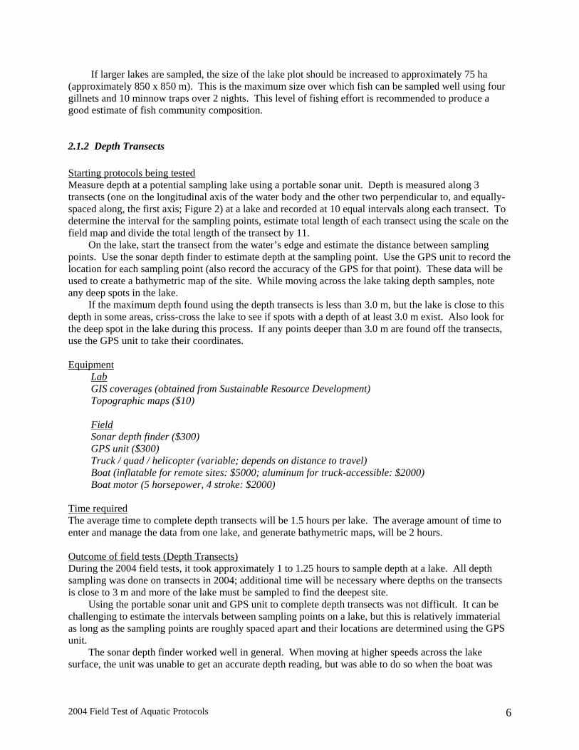
Starting protocols being tested Measure depth at a potential sampling lake using a portable sonar unit. Depth is measured along 3 transects (one on the longitudinal axis of the water body and the other two perpendicular to, and equally-spaced along, the first axis; Figure 2) at a lake and recorded at 10 equal intervals along each transect. To determine the interval for the sampling points, estimate total length of each transect using the scale on the field map and divide the total length of the transect by 11.
On the lake, start the transect from the water’s edge and estimate the distance between sampling points. Use the sonar depth finder to estimate depth at the sampling point. Use the GPS unit to record the location for each sampling point (also record the accuracy of the GPS for that point). These data will be used to create a bathymetric map of the site. While moving across the lake taking depth samples, note any deep spots in the lake.
If the maximum depth found using the depth transects is less than 3.0 m, but the lake is close to this depth in some areas, criss-cross the lake to see if spots with a depth of at least 3.0 m exist. Also look for the deep spot in the lake during this process. If any points deeper than 3.0 m are found off the transects, use the GPS unit to take their coordinates. Equipment
Lab GIS coverages (obtained from Sustainable Resource Development) Topographic maps ($10) Field Sonar depth finder ($300) GPS unit ($300) Truck / quad / helicopter (variable; depends on distance to travel) Boat (inflatable for remote sites: $5000; aluminum for truck-accessible: $2000) Boat motor (5 horsepower, 4 stroke: $2000)
Time required The average time to complete depth transects will be 1.5 hours per lake. The average amount of time to enter and manage the data from one lake, and generate bathymetric maps, will be 2 hours.
Outcome of field tests (Depth Transects) During the 2004 field tests, it took approximately 1 to 1.25 hours to sample depth at a lake. All depth sampling was done on transects in 2004; additional time will be necessary where depths on the transects is close to 3 m and more of the lake must be sampled to find the deepest site.
Using the portable sonar unit and GPS unit to complete depth transects was not difficult. It can be challenging to estimate the intervals between sampling points on a lake, but this is relatively immaterial as long as the sampling points are roughly spaced apart and their locations are determined using the GPS unit.
The sonar depth finder worked well in general. When moving at higher speeds across the lake surface, the unit was unable to get an accurate depth reading, but was able to do so when the boat was
2004 Field Test of Aquatic Protocols 7
stopped. The suction cup attached to the transducer on the portable sonar unit did not adhere well to the wooden transom of the Zodiac being used; attaching a flat metal or Plexiglas plate to the transom to provide a surface for attachment of the suction cup is a potential solution to this problem.
Figure 2. Schematic diagram of depth transects at lakes. Suggested changes to Depth Transect Protocol Depth transects should be established using GIS in the lab and a series of waypoints exported to a GPS unit. This will allow fairly precise location of sampling points by field crews, without having to visually estimate the distance between sampling points on the lake.
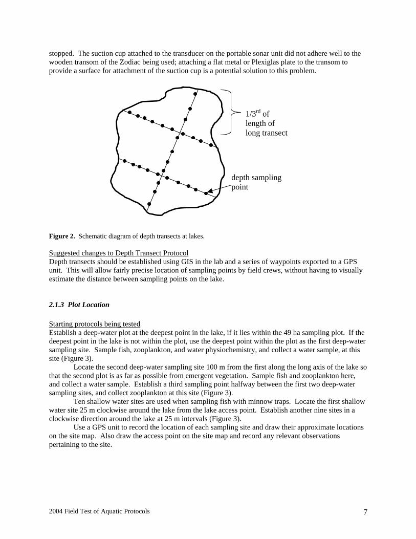
2.1.3 Plot Location Starting protocols being tested Establish a deep-water plot at the deepest point in the lake, if it lies within the 49 ha sampling plot. If the deepest point in the lake is not within the plot, use the deepest point within the plot as the first deep-water sampling site. Sample fish, zooplankton, and water physiochemistry, and collect a water sample, at this site (Figure 3).
Locate the second deep-water sampling site 100 m from the first along the long axis of the lake so that the second plot is as far as possible from emergent vegetation. Sample fish and zooplankton here, and collect a water sample. Establish a third sampling point halfway between the first two deep-water sampling sites, and collect zooplankton at this site (Figure 3).
Ten shallow water sites are used when sampling fish with minnow traps. Locate the first shallow water site 25 m clockwise around the lake from the lake access point. Establish another nine sites in a clockwise direction around the lake at 25 m intervals (Figure 3).
Use a GPS unit to record the location of each sampling site and draw their approximate locations on the site map. Also draw the access point on the site map and record any relevant observations pertaining to the site.
1/3rd of length of long transect
depth sampling point

2004 Field Test of Aquatic Protocols 8
Equipment Lab
GIS coverages to produce map of lake (obtained from Sustainable Resource Development) Field
Sonar depth finder ($300) GPS unit ($300) Truck / quad / helicopter (variable; depends on distance to travel) Boat (inflatable for remote sites: $5000; aluminum for truck-accessible: $2000) Boat motor (5 horsepower, 4 stroke: $2000)
Time required The average time required to set out the plot locations will be 1.0 hours. The average time to enter and manage the data will be 0.25 hours per site. Outcome of field tests (Plot Location) During the 2004 field tests, plot establishment was relatively simple; distances were visually estimated. Each site location was recorded using a GPS unit so actual location could be plotted. Plot establishment was integrated into other activities and did not require much time. Suggested changes to Plot Location protocol Mark the location of the plot corners temporarily with buoys; the location of the plot corners should be recorded using a GPS unit. Criss-cross the sampling plot to determine the deepest point within the plot; this will be the first deep-water sampling site. Locate a second deep-water sampling site 100 m from the first along the long axis of the lake so that the second plot is as far as possible from emergent vegetation. The marker buoys can be removed when sampling is completed.
Setting out and removing corner markers would require approximately 15 minutes. Finding the deepest point within the plot will take approximately 30 minutes. Equipment (extra or different from the initial protocol described above)
Bouys (inflatable marker buoys: $30 each x 4 = $120).
2.1.4 Water Physiochemistry Starting protocols being tested At the deepest point in the plot take vertical profiles for water temperature, pH, conductivity, and dissolved oxygen using the multiprobe meter. Record these measurements at 10 intervals from the surface to the bottom of the lake (divide the total depth by 10 and record the relevant data at the mid-point of each of these intervals).
Measure Secchi depth at the deep-water plot. Working over the shaded side of the boat, without sunglasses, lower the Secchi disk until it disappears; record the depth. Raise the disk again until it reappears and record the depth. The average of the two depths is the Secchi depth. Take the depth three times and take the average of the three depths.
Take water samples for analysis of total nitrogen, total phosphorus, and dissolved organic carbon using a clear polyethylene tube (2.54 cm inside diameter, with a one-way foot valve and an attached lead weight) extended from the lake surface to the bottom of the euphotic zone (> 1% of ambient surface light,

2004 Field Test of Aquatic Protocols 9
or approximately twice the Secchi depth) or to 25 cm above the bottom of the lake (whichever is less). Mix the water sample and collect a 250 mL subsample in a dark plastic bottle; store this sample in a cooler until it can be refrigerated. Water samples can be held for up to one month at 4° C before analysis. However, they should be shipped to the water analysis lab as soon as convenient.
Collect water samples at both deep-water plots. Wear powder-free latex or nitrile gloves when collecting water samples. Do not place hands inside or on the lip of the water sampler or sample bottles.
Figure 3. Location of sampling points at lakes, including those for fish, zooplankton, water physiochemistry, and amphibians.
Equipment Lab
Water samples should be sent to a certified lab for analysis. Costs for doing total nitrogen (TN), total phosphorus (TP), and dissolved organic carbon (DOC) is approximately $40 / sample (for all three parameters; these are the approximate charges at the University of Alberta Limnology Laboratory); therefore, if 2 samples are done per lake, the total cost per site is $80)
Lake access point
25 m
Deep –water plot
100 m
deepest point in lake
1 m depth contour
25 m
Extra zooplankton Gillnet
Minnow trap
50 m 50 m
Amphibian transect
50 m
200 m

2004 Field Test of Aquatic Protocols 10
Laboratory equipment necessary to perform the analysis for TN, TC, and DOC would cost in excess of $10,000, plus the cost of calibrating, operating, and maintaining the equipment.
Field Multiprobe meter (approximately $5500) Secchi disk ($90) clear polyethylene tube (2.54 cm inside diameter, 15 m long, with a one-way foot valve and an
attached lead weight; $55) Cooler ($50) Dark plastic bottles (usually supplied by water analysis lab; if not, cost approximately $2.50 per
250 mL dark Nalgene bottle)
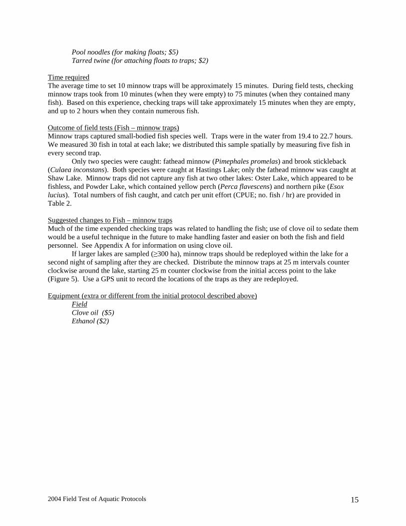
Time required The average time to measure Secchi depth will be five minutes. The average time to do a vertical profile for temperature, conductivity, dissolved oxygen, and pH will be approximately 0.25 hours, though this may increase at deeper lakes. The average time required to collect a single water sample will be five minutes. Outcome of field test (Water Physiochemistry) Taking measurements and collecting the samples for water physiochemistry was relatively easy. The multiprobe meter we had available only had a three metre cord for the probes, however, so we could not do a full vertical profile for the deeper lakes we sampled. The water samples collected during the 2004 field season were not analyzed as we were interested in how well the sampling procedures worked in the field, not the chemical status of the lakes we sampled. Therefore, analyzing the water samples would have served no purpose to the 2004 test. Suggested changes to the Water Physiochemistry Protocol Collect water for a composite sample at the deepest point in the plot and at nine other locations (see Figure 4 for locations); record each location using a GPS unit. Before taking the first water sample at a lake, rinse the sample tube and sample bottle three times with lake water, discarding the water after each rinse. Take water samples using a clear polyethylene tube (1.3 cm inside diameter, with a one-way foot valve and an attached lead weight). Extend the tube from the water’s surface to the bottom of the euphotic zone (>1% of ambient surface light, or approximately twice the Secchi depth), to 1 m above the bottom of the lake, or to 11 m deep (whichever is less). The sampling tube collects approximately 130 mL of water for every 1 m of depth. A total of at least 5 L of water should be collected. Therefore, if a lake is relatively shallow, multiple samples may be necessary at each water collection site. If this is the case, take the same number of samples at each water collection site. If the euphotic zone is deeper than 11 m, only sample the top 11 m. Wear powder-free latex or nitrile gloves during collection of water samples; do not place your hands inside, or on the lip of, the water sampler or sample bottles.
Empty each sample into a 20 L carboy placed inside a clean black garbage bag (to prevent photosynthesis from occurring within the carboy). Ensure that the bottom of the collection tube does not come any closer than 1 m to the substrate. If there is any evidence of sediment contamination of the water sample, discard the sample, rinse the tube 10 times with lake water, and take another sample. If sediment gets into the carboy, it must be emptied and rinsed 10 times with fresh lake water, and water sampling must be started all over again. After all 10 water samples are collected, mix the water by shaking the carboy vigorously and collect a 250 mL subsample in a dark plastic bottle; store this sample in a cooler until it can be refrigerated. Each water sample bottle will have a unique alphanumeric code written on it in permanent marker. Ensure that this number is recorded on the lake sample datasheet.

2004 Field Test of Aquatic Protocols 11
Increasing the number of water samples collected will increase the amount of time necessary to complete this activity. Collecting water samples (including travel between water sampling sites within the lake) should take approximately 0.75 hours. Figure 4. Suggested locations of water, zooplankton, and phytoplankton sites within lake plot (assumes a 75 ha plot). Equipment (extra or different from the initial protocol described above)
Field clear polyethylene tube (1.5 cm inside diameter, 15 m long, with a one-way foot valve and an
attached lead weight; $55) 20 L Nalgene carboy with spigot ($100)
2.1.5 Zooplankton
Starting protocols being tested Collect zooplankton samples at three sites in each lake: one at the deepest point in the lake/plot, one 50 m away from this point, and another 100 m away from the deepest point (Figure 3). During the 2004 field tests we attempted to use the collapsible tube sampler (Knoechel and Campbell 1992) which was initially recommended, but found it would not work properly. Therefore we switched to using a zooplankton net to collect zooplankton samples. Although there are problems associated with nets, such as clogging and
850 m
850 m Sample plot
275 m
275 m
Deepest point in plot
Water, zooplankton, and phytoplankton sampling point

2004 Field Test of Aquatic Protocols 12
variable filtering efficiency, zooplankton nets are simple to use and take up much less space than tube samplers, making them more attractive for working in remote sites.
Collect samples by allowing the net to sink within 25 cm of the bottom of the lake, and then drawing it up steadily to the surface. Rinse zooplankton down into the sample bucket using a squeeze bottle filled with lake water; make sure the water is only sprayed onto the net from the outside, to ensure additional zooplankton are not introduced to the sample. Immerse the zooplankton in carbonated water for one minute to narcotize them, then preserve them in 4% buffered formalin-sucrose solution.
Different amounts of water are sampled in lakes of different depths. Because the accumulation of species is not linear with effort, sampling must be standardized. This can be accomplished by only sampling to a given depth of water (e.g. 2 m) in all lakes, but this approach would miss many species that might occur at greater depths. Therefore, sampling is done to near the bottom of the lakes, so that most species occurring in the lake are available to be sampled during the subsampling step. Subsampling consists of filtering zooplankton from the preservative and adding them to 1000 mL of water in an Imhoff cone. A given volume of water is then removed from the cone. This volume is based on a ratio of 1:10 sample to original depth of lake for a lake 10 m deep: 100 mL would be withdrawn from the cone if a depth of 10 m of water was originally sampled. For depths <10 m, a greater volume of water is withdrawn from the Imhoff cone to achieve the same relative sampling effort. Zooplankton samples are further subsampled during identification, if the samples contain high numbers of individuals.
Equipment Lab Imhoff cone ($125) Filtering equipment ($5) Chemicals ($1)
Microscope, sample splitter, taxonomic keys (samples should be sent to consultants for processing, so this equipment will be unnecessary)
Field Zooplankton net (during initial tests we used one available at ARC; see section on suggested
changes below for recommendations for type of net to use in future) Sample bottles ($5) Narcotizing agent (Eno, Alka-Seltzer, etc.: $0.25) Squeeze bottle (1 L; $8) Chemicals ($1)
Time required The average time to collect each zooplankton sample will be 15 minutes. The average time to prepare each sample (including standardizing the sample using the Imhoff cone) for shipping to the consultants for identification will be 30 minutes per sample. The average amount of time to enter and manage the data from each site will be 15 minutes. Outcome of field test (zooplankton tube sampler) We initially constructed a collapsible tube sampler from a flexible dryer hose and other materials as described by Knoechel and Campbell (1992). Unfortunately, we had persistent problems with leakage, failure of the closing mechanism when drawing the tube out of the water so that the entire sample escaped, and the bulk of the sampler. After several trials we decided that the tube sampler was too cumbersome and the potential for problems with the unit was too high to continue its use.

2004 Field Test of Aquatic Protocols 13
Outcome of field test (zooplankton net) The only zooplankton net available at ARC was large (diameter of 0.5 m), but served to demonstrate the length of time required to sample zooplankton (10 – 15 minutes per sample), and other logistic and procedural considerations
Zooplankton samples were obtained from two lakes (Shaw and Powder). Sampling was attempted in a third lake (Oster) using the tube sampler, but this sample was not analyzed because the sampling equipment was inadequate. During attempts to obtain a zooplankton sample from a fourth lake (Hastings) the bottom of the straining bucket on the zooplankton net broke off the bucket and was lost in the lake and the net could no longer be used.
Zooplankton samples were sent to a private consultant for identification. Few species were present in the two lakes sampled, though the species found in each lake were different (Table 1); Shaw Lake had much higher zooplankton densities than did Powder Lake. Other studies have found much higher zooplankton diversity in Alberta. Anderson and Green (1976) found a mean of 19 species of crustacean and 12 species of rotiferan zooplankton in the Waterton Lakes in Waterton National Park, Alberta. Twenty-four zooplankton species were found in North Halfmoon and Lofty Lakes, Alberta, over a three-year period (1991 – 1993; Ghadouani et al. 1998). Thirty-three species were found in Halfmoon, Lofty, Crooked, and Jenkins Lake in 1990 (Pinel-Alloul 1993). Studies of zooplankton in North American lakes indicate that average local (lake scale) richness can vary from 5.5 to 11.3 species, while regional richness can vary from 9 to 69 species; note that these figures are based on 20 different studies which sampled at least 20 lakes each, and that the species richness values do not include rotifers (Shurin et al. 2000). Table 1. Zooplankton species found in sample lakes, 2004. Group Species Mean no. individuals / L (SD); n = 3 Shaw Lake Powder Lake Calanoida Leptodiaptomus siciloides 2.18 (1.5) 0 Leptodiaptomus minutus 0 0.40 (0.35) Cyclopoida Dicyclops thomasi 1.31 (0.94) 0 cyclopoid copeopod 0 0.05 (0.03) Caldocera Daphnia longiremis 23.7 (10.8) 0 Daphnia retrocurva 0 0.92 (0.76) Bosmina longirotris 3.46 (2.03) 0 Diptera Chaoborus sp. 0.43 (0.34) 0 Amphipoda Gammarus lacustris 0.01 (0.0046) 0 Oligochaeta Pristina sp. 0 0.01 (0.01)
Suggested changes to Zooplankton collection protocol In the future, a Wisconsin-style net 75 cm long with an opening of 13 cm and a detachable straining bucket should be used. Mesh size of the net should be 63 µm. Soak the net in the lake for 2 minutes before use. Before taking the zooplankton haul, fill a Nalgene squeeze bottle with water filtered through the net. Lower the net vertically to the bottom of the euphotic zone, or to within 1 m of the bottom (don’t forget to account for the length of the net), whichever is less. The net should be retrieved at a rate of approximately 0.5 m/s so that fast-swimming zooplankton cannot avoid the net. Upon completing the haul, pull the rim of the net above the surface of the lake and splash water onto the outside of the net (not into the net) to wash the zooplankton down into the sample bucket. When this has been completed, remove the sample bucket from the net, hold the tube at the bottom over a sample bottle, open the tube

2004 Field Test of Aquatic Protocols 14
and allow the sample to drain into the bottle. Use the squeeze bottle previously filled with water to rinse the entire sample down into the bottle. Add Eno or Alka-Seltzer to narcotize the zooplankton, and then add buffered formalin in sufficient quantity (about 5% of the total volume of the sample) to preserve the sample. Make sure the depth of water sampled at each site is recorded.
Single samples may not provide good estimates of zooplankton species richness in a lake; additional samples improve estimates of the annual species pool (Arnott et al. 1998). In one lake where spatial variation in species richness was estimated by sampling at 10 different stations, cumulative species richness leveled off at approximately nine samples in three of the four months in which sampling was done (Arnott et al. 1998). Another study indicated that single samples were able to capture at least 80% of the zooplankton species present in a lake only in small lakes, while this was not achieved in larger lakes until approximately nine samples had been taken (Patalas and Salki 1993). In contrast, Stemberger et al. (2001) suggested that a single vertical haul at the deepest point a lake was sufficient for trend detection, although this approach did not provide sufficient information for status estimation. I suggest that 10 vertical hauls (one at the deepest point in the lake / plot, and the remaining nine at the same stations were additional water physiochemistry samples are taken) be made in each lake. Pool the samples taken at the 10 sites before subsampling and sending the zooplankton to an expert consultant for identification. The approximate cost of identification will be $150/sample. Equipment (extra or different from the initial protocol described above)
Field Zooplankton net (Wisconsin-style net 75 cm long with an opening of 13 cm and a detachable
straining bucket; mesh size of the net should be 63 µm: $500) 2.1.6 Fish – minnow traps Starting protocols being tested Set 10 minnow traps (standard Gee minnow traps with 6.35 m mesh) in each lake. Set traps on the bottom of the lake along the 1 m depth contour at intervals of 25 m clockwise around the lake, starting 25 m from the lake access point (Figure 3). Use a GPS unit to record the location of each trap. Mark traps with lengths of pool noodle tied to the traps. Set traps during the afternoon and retrieve them the following day.
Check traps one at a time and empty them into a live well (bucket with fresh lake water); remove fish from the live well in batches using a small net (e.g. aquarium net) and assign each individual to a species. Release all fish back into the lake of origin, unless collecting voucher specimens. See Appendix A for information on fish processing, preservation of samples, and disposal of dead fish.
Equipment Lab Bottles (1 L; $15) Isopropyl alcohol (70%; $10)
Field Bottles (1 L; $15) Isopropyl alcohol (70%; $10) Portable electronic balance (10,000 g capacity, 1 g readability: $450) 30 cm fish measuring board ($75) Live well (bucket or plastic bin; $25) Net (aquarium net; $5) Gee minnow traps (6.35 mm mesh; $200)
2004 Field Test of Aquatic Protocols 15
Pool noodles (for making floats; $5) Tarred twine (for attaching floats to traps; $2) Time required The average time to set 10 minnow traps will be approximately 15 minutes. During field tests, checking minnow traps took from 10 minutes (when they were empty) to 75 minutes (when they contained many fish). Based on this experience, checking traps will take approximately 15 minutes when they are empty, and up to 2 hours when they contain numerous fish. Outcome of field tests (Fish – minnow traps) Minnow traps captured small-bodied fish species well. Traps were in the water from 19.4 to 22.7 hours. We measured 30 fish in total at each lake; we distributed this sample spatially by measuring five fish in every second trap.
Only two species were caught: fathead minnow (Pimephales promelas) and brook stickleback (Culaea inconstans). Both species were caught at Hastings Lake; only the fathead minnow was caught at Shaw Lake. Minnow traps did not capture any fish at two other lakes: Oster Lake, which appeared to be fishless, and Powder Lake, which contained yellow perch (Perca flavescens) and northern pike (Esox lucius). Total numbers of fish caught, and catch per unit effort (CPUE; no. fish / hr) are provided in Table 2. Suggested changes to Fish – minnow traps Much of the time expended checking traps was related to handling the fish; use of clove oil to sedate them would be a useful technique in the future to make handling faster and easier on both the fish and field personnel. See Appendix A for information on using clove oil. If larger lakes are sampled (≥300 ha), minnow traps should be redeployed within the lake for a second night of sampling after they are checked. Distribute the minnow traps at 25 m intervals counter clockwise around the lake, starting 25 m counter clockwise from the initial access point to the lake (Figure 5). Use a GPS unit to record the locations of the traps as they are redeployed. Equipment (extra or different from the initial protocol described above)
Field Clove oil ($5) Ethanol ($2)

2004 Field Test of Aquatic Protocols 16
Table 2. Results from fish sampling with minnow traps and gillnets. Oster Lake (Elk Island National Park) was also sampled with minnow traps and gillnets, but no fish were caught.
Lake Species Total no. caught
Mean (StDev) no. per trap
Mean CPUE (StDev) (no./hr)
N (number of gear)
Minnow traps
Shaw Lake Fathead minnow 208 20.8 (15.8) 0.95 (0.72) 10
Hastings Lake Fathead minnow 779 77.9 (65.9) 3.9 (3.31) 10
Hastings Lake Brook stickleback 151 15.1 (12.6) 0.74 (0.61) 10
Gillnets
Shaw Lake Fathead minnow 26 6.5 (7.0) 0.29 (0.32) 4
Hastings Lake Fathead minnow 153 38.2 (38.6) 1.8 (1.8) 4
Hastings Lake Brook stickleback 37 9.2 (6.4) 0.44 (0.30) 4
Powder Lake Northern Pike 43 10.8 (4.4) 0.46 (0.20) 4
Powder Lake Yellow Perch 134 33.5 (10.6) 1.5 (0.52) 4
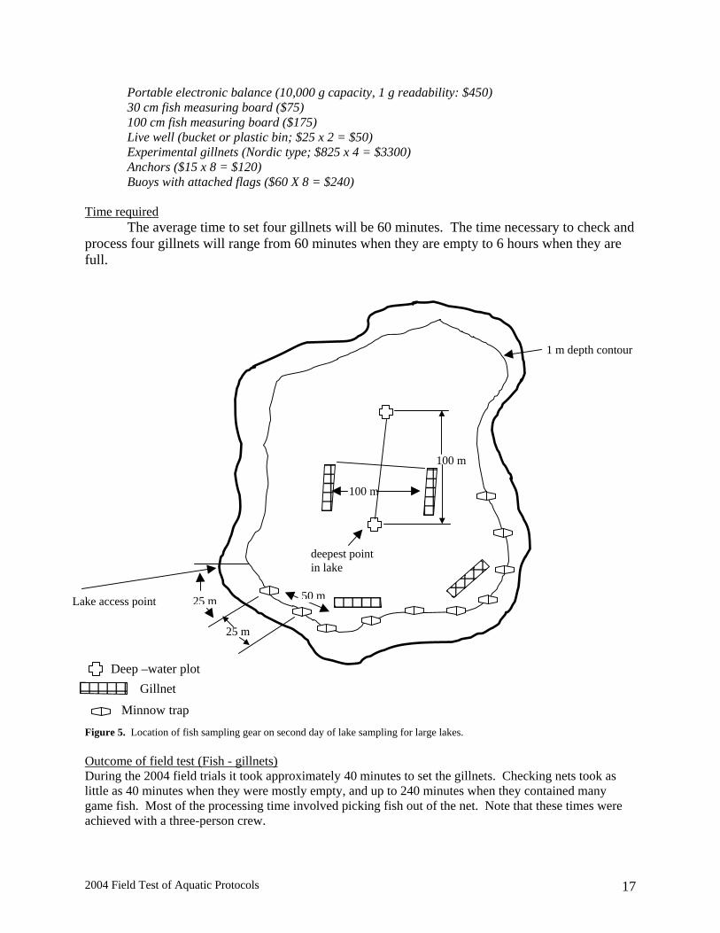
2.1.7 Fish – gillnets Starting protocols being tested Set four gillnets in each lake. Gillnets are 30 m long and consist of 12 panels, each 2.5 long x 1.5 m high. Mesh sizes of the panels range from 5 to 55 mm (knot-to-knot measurement). Set two nets in relatively deep water (up to 6 m deep), 100 m apart (Figure 3). Set the remaining two nets closer to shore, in water 1.5 to 2 m deep, offshore of the minnow traps, with one gillnet 50 m clockwise from the first minnow trap, and the second set 50 m counter clockwise from the last minnow trap (Figure 3).
Secure the bottoms of the gill nets (the leadlines) in position with anchors, and attach the tops (the float lines) to buoys. Set gillnets during the afternoon and retrieve them the following day. Process captured fish as for those caught in minnow traps.
Many fish captured in gillnets will die. Collect ageing structures from at least 30 specimens of each species of game fish. See Appendix A for guidelines on fish handling, preservation, collection of ageing structures, and disposal.
Equipment Lab Bottles (1 L; $15) Isopropyl alcohol (70%; $10) Coin envelopes ($3) Scissors ($4)
Field Bottles (1 L; $15) Isopropyl alcohol (70%; $10)
2004 Field Test of Aquatic Protocols 17
Portable electronic balance (10,000 g capacity, 1 g readability: $450) 30 cm fish measuring board ($75) 100 cm fish measuring board ($175) Live well (bucket or plastic bin; $25 x 2 = $50) Experimental gillnets (Nordic type; $825 x 4 = $3300) Anchors ($15 x 8 = $120) Buoys with attached flags ($60 X 8 = $240) Time required
The average time to set four gillnets will be 60 minutes. The time necessary to check and process four gillnets will range from 60 minutes when they are empty to 6 hours when they are full.
Figure 5. Location of fish sampling gear on second day of lake sampling for large lakes. Outcome of field test (Fish - gillnets) During the 2004 field trials it took approximately 40 minutes to set the gillnets. Checking nets took as little as 40 minutes when they were mostly empty, and up to 240 minutes when they contained many game fish. Most of the processing time involved picking fish out of the net. Note that these times were achieved with a three-person crew.
Lake access point
Deep –water plot
100 m
deepest point in lake
1 m depth contour
25 m
Gillnet
Minnow trap
50 m25 m
100 m

2004 Field Test of Aquatic Protocols 18
Gillnets captured both small-bodied (minnows, stickleback) and large-bodied (perch, pike) fish species. Total numbers of fish caught, and catch per unit effort (CPUE; no. fish/hr) are provided in Table 2. Nets were in the water from 20.95 to 25.08 hours.
Multimesh gillnets require more gear to set up than minnow traps, and are themselves greater in bulk because they must be carried in plastic tubs. A competent boat operator is required when setting nets, to ensure they remain taut. Two anchors are required for each net; 5 – 10 lb cannon ball anchors require the least room for transport, compared other types of anchors. Each net also requires two buoys with flags (see Appendix B, Regulations for marking nets and traps), one at either end of the net. These buoys require a large amount of space for transport. Suggested changes to Fish – gillnets The deployment of gillnets was changed at the start of the field season from the initially-proposed protocols (where the first littoral gillnet was to be set 100 m counter clockwise from the first minnow trap) to make setting and checking the fish sampling gear more efficient. The majority of time spent checking gillnets was for removing fish from the nets. This was more difficult when the fish was alive and struggling. Use of an anaesthetic, such as clove oil (see Appendix A) would make removal of fish from the net easier, and reduce the stress experienced by the fish. Costs and time required to use clove oil would be similar to those estimates provided in the minnow trap section above. If larger lakes are sampled (≥300 ha), redeploy the gillnets within the lake for a second night of sampling after checking them. Move the two deep gillnets to sites located 100 m on either side of a line drawn between the two deep-water plots (Figure 5); deploy the gillnets parallel to the long axis of the lake. Set the two shallow gillnets in proximity to the minnow traps (after the minnow traps have been moved). Set one gillnet 50 m clockwise from the first minnow trap, and the second 50 m counter clockwise from the last minnow trap (Figure 5).
2.1.8 Amphibians Starting protocols being tested Sample amphibians using low-intensity area-constrained surveys: search a pre-determined area for all amphibians, but do not search under fallen logs, leaf litter, and other debris (Crump and Scott 1994). Before beginning the survey, record air temperature and weather conditions (cloud cover, wind speed, precipitation), as these factors may influence amphibian activity. Start visual survey transects 50 m in either direction (clockwise and counter clockwise around the lake) from the point at which the lake is accessed (Figure 3).
Visual survey transects are 1 m wide x 200 m long, and within 3 – 5 m of the lakeshore. In cases where the transect cannot be done this close to the lake, because the bank is unstable, there are floating vegetation mats around the lake, or the edge of the lake is obscured by tall reeds or other vegetation, record the approximate distance between the lakeshore and where the transect was actually done. One person will do each transect.
At the beginning of the transect record the start time and the starting position using a GPS unit. Walk slowly along the transect, staying as parallel to the shoreline as possible, scanning the ground in front along a 1 m wide band. While walking along the transect note all amphibians observed, including species and age class (young-of-the-year, adult), if possible. Whenever possible, capture each amphibian; all amphibians captured should be identified to species and released at the capture point or at the end of the transect. Where amphibians are abundant it is more efficient to hold all the animals captured and process them once the survey has been completed. When time is available, measure and weigh the first 30 individuals of each species; if possible, all individuals should be examined for deformities and parasites.

2004 Field Test of Aquatic Protocols 19
Record the time when the transect is completed and any general observations pertaining to the survey conditions, such as “high grass, difficult to see” or “heard many chorus frogs calling nearby but were unable to see any”. Use a GPS unit to record the end point of the transect.
Equipment
Field GPS unit ($300) 50 m measuring tape ($60) Flagging tape ($5) Plastic bags ($1) Plastic ruler ($0.25) Pesola spring scale (60 g with 0.5 g increments; $75) Time required The average time necessary to complete amphibian transects will be approximately 45 minutes (including time to process amphibian captures); this will vary with the complexity of the habitat being surveyed (e.g. a wooded area with abundant downed trees vs. a grassy meadow), and the number of amphibians captured. The time required to enter and manage the data from one site will be approximately 15 minutes. Outcome of field test (Amphibians) During the 2004 field tests amphibian surveys took approximately 15 to 20 minutes per transect; time to search a transect varied with shoreline conditions and the number of amphibians seen and captured.
Sampling conditions varied from open shoreline with high grass and bulrushes (Powder Lake) to heavily wooded, sloping shores frequently cut with animal runs and abundant blowdown (Shaw Lake). The former was physically much easier to sample than the latter, but the amount of time to sample at each lake was roughly similar as amphibians were relatively abundant at Shaw Lake (7 amphibians on one transect, 19 on the second), while none were seen at Powder Lake. Amphibians were not sampled at the other two lakes due to time constraints. The only species observed were the wood frog (Rana sylvatica), and boreal chorus frog (Pseudacris triseriata).
One problem encountered during amphibian surveys was trying to estimate the distance travelled during the survey. During the field trials in 2004 we used measured paces to estimate the distance; I have used this method in a number of forested areas, and have found it to be reasonably close to measured distances. Suggested changes to Amphibian survey protocol
I recommend that amphibian surveys be dropped from the lake sampling protocols and added instead to the stream and wetland sampling protocols. This will generate more detailed data on the distribution of this group across the province. Suggested additions to lake sampling protocol 2.1.9 Phytoplankton Collect 1 L of water from the carboy filled when collecting water for chemical analysis. Use an opaque polyethylene bottle to collect and store the sample. Immediately after collection add 10 mL of Lugol’s solution (recipe: 100 g iodine, 200 g potassium iodine, 200 mL glacial acetic acid, and 2000 mL distilled water) to the sample, followed immediately by 20 mL of FAA (recipe: equal volumes of formaldehyde [37%] and glacial acetic acid). Store the sample bottle in the dark.

2004 Field Test of Aquatic Protocols 20
Equipment
Field Opaque plastic bottles ($4.00 per 1 L amber polypropylene bottle) Chemicals ($1.00)
Time required The average time required to sample to collect and preserve phytoplankton samples at a single site will be 10 minutes. The time required to identify phytoplankton from one site would vary substantially with the training and experience of the taxonomist; a contract will be established to identify the specimens. The approximate cost for identification will be $150/sample. Time required to enter and manage the data from a site will be 30 minutes. 2.1.10 Summary of suggested changes to protocols for lakes Rather than sampling lakes at regional scales, fewer (approximately 100) and larger (≥300 ha in size) lakes should be targeted to obtain a provincial-scale indication of lake biodiversity. Information on the depth of lakes should be sought wherever possible before the lake is actually visited to reduce the number of visits to lakes that are too shallow. Sampling plot size on lakes should be set at 75 ha to ensure fish can be adequately sampled using the recommended sampling effort of 10 minnow traps and four gillnets set over two nights. A composite water sample should be taken by collecting water at 10 sites, combining the samples, and taking a subsample. A subsample of the same water can be collected for phytoplankton. Slight adjustments were made during 2004 field tests in the location of the littoral gillnets to make deploying and checking the gear more efficient; this should be continued. Clove oil should be used to anaesthetize live fish to reduce handling stress and to make it easier to measure them and extract them from nets. The method for sampling zooplankton was changed from a tube sampler to a net to improve reliability and portability of sampling gear; use of a net for zooplankton net should continue. Amphibians should no longer be sampled at lakes; they should be sampled at streams and wetlands instead.
2.2 FLOWING WATER PROTOCOLS
2.2.1 Stream Selection Starting protocols being tested
For testing aquatic sampling protocols in 2004, chosen streams were accessible by land, and took less than 2 hours to reach from base camp. Streams were chosen based on flow (impounded areas were avoided) and depth (had to be safely wadeable). During actual implementation of the ABMP, however, potential streams closest to an ABMP terrestrial sampling point will be identified using GIS and air photos, and visited to verify that they are acceptable as sampling sites.
Locating acceptable sites (streams with a depth of at least 25 cm, but no more than 1.5 m; width of at least 1 m) may be problematic. GIS layers contain little data on parameters such as stream width (except for larger streams), and it is difficult to determine if streams are ephemeral or persistent based on GIS data. Beavers will continue to provide challenges to the stream program, as their impact from one sampling period to the next will be unpredictable. Impoundment of a stream reach by beavers drastically changes the character of the stream in that area, changing erosional / depositional patterns, benthic invertebrate communities, and physical characteristics of the stream (e.g. depth, width, flow rate).

2004 Field Test of Aquatic Protocols 21
Equipment Lab GIS coverages (obtained from Sustainable Resource Development) Topographic maps ($10) Field Folding 2 m measuring stick ($20) 50 m measuring tape ($60) Truck / quad / helicopter (variable; depends on distance to travel)
Time required The average time required to identify possible stream sites and access routes using GIS and maps in the lab will be 2 hours. Average time to reach and check each potential site in the field will be 2 hours. Outcome of field tests (Stream Selection) Site selection was a challenge in 2004. Potential streams were identified using topographic and GIS-generated maps. In the Lac La Biche area only two suitable streams were found out of eight that were assessed. In the Grand Prairie area, three suitable streams were sampled to test protocols. Suggested changes to Stream Selection Protocol In the future I suggest that streams be sampled only in the foothill and Rocky Mountain ecoregions. Beaver-affected stream reaches should be avoided. Although it is possible to sample benthic macroinvertebrates in beaver-impounded areas, the sampling methods that are used are different from those used in flowing water and the benthic macroinvertebrate community will be very different from that of a stream with flowing water; therefore, it would be difficult to compare data collected at sites with running water, and those with standing water. Behind beaver dams the benthic community shifts to resemble one typical of lentic, rather than lotic, systems. As lentic waters are being sampled both as lakes and wetlands it seems redundant to sample beaver ponds. Therefore I suggest that streams that contain flowing water be sampled so that the type of habitat being sampled remains consistent. If a site becomes beaver-impounded between sampling visits, a different site with flowing water up or downstream from the former site should be identified and sampled. I suggest that the variation introduced by such an action is less than would be introduced by sampling the same site as flowing water in one sampling round, and as a beaver pond at the next sampling event. I recommend sampling streams in the Rocky Mountains and foothills because streams are probably the predominant aquatic habitat in these areas of relatively high relief. This approach will provide regional-scale data on streams in these ecoregions. As mentioned above, I recommend sampling rivers to provide data on flowing water habitats at a provincial scale. By sampling rivers, problems associated with beavers can be avoided in some areas of the province (e.g. boreal forest) where they are numerous and most streams are dammed. 2.2.2 Plot Location Starting protocols being tested At each stream site, establish five cross-section plots. Establish the first plot 25 m upstream from where the team first reached the stream; identify this first plot with a steel bar driven into the ground next to the stream; mark it’s location with flagging tape. Establish four more plots at 50 m intervals upstream of the first plot; mark them with flagging tape (Figure 6). Record the location of each plot with a GPS unit.

2004 Field Test of Aquatic Protocols 22
Equipment Field 50 m measuring tape ($60) Steel bar ($5) Flagging tape ($5) Mallet ($20)
Figure 6. Schematic diagram of stream sampling protocols, 2004. Time required The average amount of time required to establish plots along streams will be 15 minutes. Plot establishment will be integrated with other activities, so a plot will be located, marked with flagging tape, and then sampled; after sampling, the crew will move on to the next plot, sample it, and so on. Outcome of field tests (Plot Location) Delineating the plots was usually not problematic during field tests, and took relatively little time. The only major problem sometimes encountered was moving between sampling plots when riparian vegetation was thick or water was relatively deep.
Suggested changes to Plot Location Protocol The protocol tested in 2004 was a slight modification of the initial protocol, in which the first plot was established in the middle of the sampled reach, with two plots upstream and two plots downstream from the first plot. The change to establish all 5 transects upstream of the stream access point was made to increase the efficiency of stream sampling. This approach should continue in the future.
Access point
25 m
50 m
50 m
50 m
50 m
Stream flow
Plot and DWM
Depth and substrate
Substrate
Benthic invertebrates
0.25 m

2004 Field Test of Aquatic Protocols 23
2.2.3 Physical Characteristics of Streams
Starting protocols being tested At each plot measure the following parameters: (a) bankfull width (width of the channel at the point where over-bank flow begins during a flood event; may be discerned by the lower extent of perennial vegetation, and / or changes in slope or particle size of the stream bank); (b) wetted width (width of the channel presently containing water); (c) maximum depth (if the water is too deep to wade a section, then record that the water is deeper than x [e.g. 1.5 m]); (d) depth at 25%, 50%, and 75% of the wetted width. Make a sketch of the channel between the first and last cross-section plot, including the location of the sample plots and concentrations of downed woody material (DWM). The sketch can be made by standing on the bank at the cross-section farthest upstream and looking downstream and making the sketch, and then moving to the cross-section farthest downstream and looking upstream to verify the initial sketch. At each of the five cross-sections, visually estimate the proportion of the substrate in six fraction classes in a 1 m band across the stream. The six fraction classes are bedrock (>4000 mm), boulders (>250 – 4000 mm), cobble (>64 – 250 mm), gravel (>2 – 64 mm), sand (>0.06 – 2 mm), and fines (<0.06 mm).
At each cross-section count and measure (length and diameter where the DWM intersects the cross-section) all pieces of downed wood material (DWM) > 1 cm across that intersect the cross-section. If the water is too deep to measure the DWM directly, estimate these measurements (record that they are estimated and why). If the bottom of the channel is not visible, do not do a DWM survey: record the length of the cross-section that was not surveyed and why this occurred.
Equipment
Field 50 m measuring tape ($60) Aluminum 24 inch DBH calipers ($225)
Time required The average time necessary to complete the surveys for DWM and substrate will be 2 hours. The time to enter and manage the data for one site will be 30 minutes. Outcome of field tests (Physical Characteristics of Streams) During the 2004 field tests measuring and characterizing parameters at stream cross-sections took approximately 15 minutes per cross section. Most aspects of the protocol for describing the physical characteristics of streams worked well, with modifications. In the field characterization of substrates was changed from a series of circular plots across the stream (the initial protocol) to a 1 m band across the transect; this provided a better indication of the substrate of the stream reach as a whole, and avoids problems of plots overlapping in narrow streams. At test streams the cross-sectional transects missed all DWM in the stream, even though it was relatively abundant in most cases. Suggested changes to Physical Characteristics of Streams Protocol In the future, the location and extent of riffle, run, and pool habitats should be included in the site sketch of the stream. In addition, the proportion of the stream that is represented by riffles, runs, glides, and pools should be visually estimated for a 1 m band across the stream at each cross-section.
Characterization of substrates should continue to be done as a 1 m wide band across the stream, as described above. This is a slight change in protocol from that initially suggested, in which size fractions were visually estimated 1 m circumference circle at five locations (0%, 25%, 50%, 75% and 100% of wetted width) across each cross-section. This change was made to increase the efficiency of describing the substrate, and providing a better characterization of the stream bottom. Another change

2004 Field Test of Aquatic Protocols 24
was that in cases where the substrate could not be seen (due to turbidity or turbulence) substrate size was assessed by feel with hands or feet.
In the future DWM should be measured along 1 m wide transects extending along the length of the stream between the first three cross-sectional transects with the first DWM transect at 25%, the second at 50%, and the third at 75% of the wetted width (Figure 7). Count and measure the length of all pieces of downed woody material (DWM) > 1 cm across that enter the 1 m width of the transect and measure the diameter of the DWM in the middle of its length.
Figure 7. Schematic diagram of stream showing revised location of downed woody material (DWM) transects and cross-sectional stream transects.
A number of elements should be estimated for a 20 m segment of bank centered at the end of each transect. Elements that should be estimated include stream bank stability (see Table 3; make notes on the cause of any instability, such as road crossing, cattle watering, or undercutting), dominant riparian vegetation (living vegetation within 5 m of stream; categories = none, grass/sedge, shrub, deciduous, coniferous, and mixedwood), and terrestrial canopy cover (living vegetation that projects over water surface; this can be any vegetation from grass to trees; categories = none, low, moderate, high). A densitometer should be used to measure tree / shrub canopy cover when standing in the middle of the stream at each transect. Substrate embeddedness when characterizing substrate composition (categories = none [<25% of large substrate types covered in fines], low [26 – 50%], moderate [51-75%], and high [>75%]). The slope of the stream reach sampled should be determined in the lab using a digital elevation model (DEM) in ArcMap. Equipment (extra or different from the initial protocol described above)
Field Densitometer ($200)
Access point
25 m 50 m
Stream flow
Transect
DWM
2004 Field Test of Aquatic Protocols 25
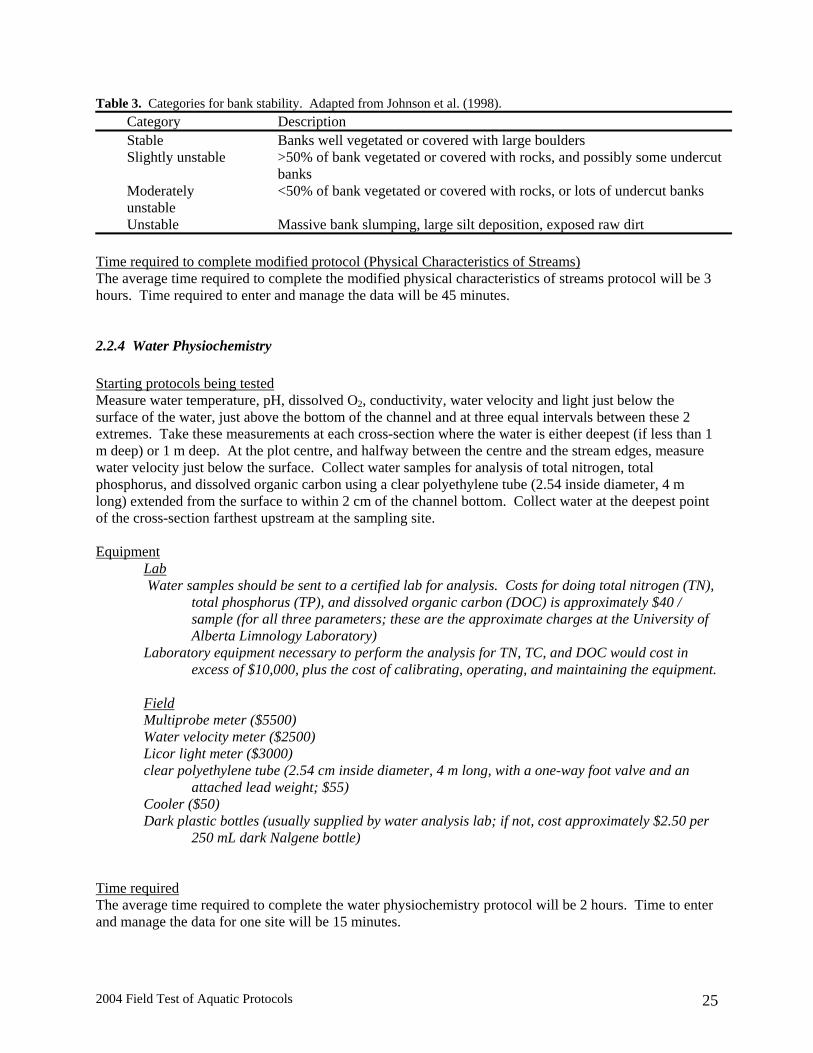
Table 3. Categories for bank stability. Adapted from Johnson et al. (1998). Category Description Stable Banks well vegetated or covered with large boulders Slightly unstable >50% of bank vegetated or covered with rocks, and possibly some undercut
banks Moderately unstable
<50% of bank vegetated or covered with rocks, or lots of undercut banks
Unstable Massive bank slumping, large silt deposition, exposed raw dirt Time required to complete modified protocol (Physical Characteristics of Streams) The average time required to complete the modified physical characteristics of streams protocol will be 3 hours. Time required to enter and manage the data will be 45 minutes. 2.2.4 Water Physiochemistry Starting protocols being tested Measure water temperature, pH, dissolved O2, conductivity, water velocity and light just below the surface of the water, just above the bottom of the channel and at three equal intervals between these 2 extremes. Take these measurements at each cross-section where the water is either deepest (if less than 1 m deep) or 1 m deep. At the plot centre, and halfway between the centre and the stream edges, measure water velocity just below the surface. Collect water samples for analysis of total nitrogen, total phosphorus, and dissolved organic carbon using a clear polyethylene tube (2.54 inside diameter, 4 m long) extended from the surface to within 2 cm of the channel bottom. Collect water at the deepest point of the cross-section farthest upstream at the sampling site. Equipment Lab
Water samples should be sent to a certified lab for analysis. Costs for doing total nitrogen (TN), total phosphorus (TP), and dissolved organic carbon (DOC) is approximately $40 / sample (for all three parameters; these are the approximate charges at the University of Alberta Limnology Laboratory)
Laboratory equipment necessary to perform the analysis for TN, TC, and DOC would cost in excess of $10,000, plus the cost of calibrating, operating, and maintaining the equipment.
Field Multiprobe meter ($5500) Water velocity meter ($2500) Licor light meter ($3000) clear polyethylene tube (2.54 cm inside diameter, 4 m long, with a one-way foot valve and an
attached lead weight; $55) Cooler ($50) Dark plastic bottles (usually supplied by water analysis lab; if not, cost approximately $2.50 per
250 mL dark Nalgene bottle) Time required The average time required to complete the water physiochemistry protocol will be 2 hours. Time to enter and manage the data for one site will be 15 minutes.

2004 Field Test of Aquatic Protocols 26
Outcome of field test (water physiochemistry) Measuring water physiochemistry at stream sections took little time (<10 minutes / section) during the 2004 field test. No water samples were collected in 2004, but collection of water samples is expected to be rapid (< 5 minutes / sample).
No light meter was available for use in 2004, so this parameter was not measured. No problems are anticipated with operation of a light meter in streams. Streams often proved too shallow for measurements of water temperature, pH, dissolved O2, conductivity, and water velocity to be made at the bottom, middle, and top of the water column at each position (25%, 50%, and 75%) across the stream to be meaningful.
Suggested changes to Water Physiochemistry Protocol In the future the number of times that flow, dissolved oxygen, pH, temperature, and conductivity will be measured at each transect across a stream will be reduced. These measurements should be taken in the middle of the water column at 25%, 50%, and 75% of the stream width. Measurements of light in the stream will be dropped.
When taking the water sample, collect at least 5 L of water; use the water sampling tube more than once if necessary. Mix the water sample and collect a 250 mL subsample in a dark plastic bottle. Make sure to wear Nitrile gloves while collecting water samples and always rinse the bottle out three times with water before taking the sample. Store water samples in a cooler until they can be refrigerated. Water samples can be held for up to two months at 4° C before analysis. Time required to complete modified protocol (Water Physiochemistry) The average time required to complete the modified water physiochemistry protocol will be 1.5 hours. Time required to enter and manage the data for one site will be 15 minutes.
2.2.5 Benthic Macroinvertebrates
Starting protocols being tested Initial protocols suggested that benthic macroinvertebrates should be sampled using a Neill sampler, with two samples taken at each stream cross-section: one in the middle of the cross-section, and one halfway between the middle and the stream bank. Samples were to be offset from the cross-sections by 25 cm upstream. The kind of habitat in which each sample is taken (run, riffle, pool), as well as the substrate sampled (silt, sand, gravel, cobble, bedrock), was to be recorded.
Given the size and weight of the Neill sampler, and the fact that it would not work well on some substrates, the initial protocol was changed to use a D-frame kick net to sample macroinvertebrates. An area as wide as the frame of the kick net and twice as long is agitated by hand or foot for 60 seconds while the net is held downstream to capture any dislodged invertebrates. Samples are taken 25 cm upstream from the cross-sectional transects. At the first transect, one sample is taken at 25% of the stream width, while the other is taken in the middle of the transect (Figure 6). As sampling proceeds upstream, the side sample switches between 25% and 75% of the stream width, but a sample is always collected in the middle of the stream.
Material collected in the kick net is placed in sample bottles and preserved with 70% ethanol for transport to the lab. A label including date, site, collectors, collection gear, and transect / sample plot data is written in pencil on a piece of paper and included inside the bottle.
In the lab the benthic invertebrates are picked from the other material in the sample (e.g. plant fragments and other debris); this may be accomplished by passing the sample through a series of sieves and using dissecting microscopes. Picked samples are placed in sample bottles with the original labels until identification of the invertebrates can be done.

2004 Field Test of Aquatic Protocols 27
Specimens should be identified to the lowest possible level (genus or species, preferably). The taxonomy of most invertebrate groups is complex and successful identification requires extensive training and experience. Given these factors, and the fact that errors in identification increase when finer taxonomic levels are approached, benthic macroinvertebrate samples should be sent to consultants for identification. Consultants charge from $60 to $500 to identify benthic macroinvertebrates from samples that have already been picked and sorted to coarse taxonomic groups (e.g. Family). Equipment Lab Sample bottles ($10) Ethanol ($3) Microscope ($6000) Counting equipment (forceps, petri dishes, etc; $20) Sieves ($90 x 3 different sizes = $270)
Field Sweep net (modified D ring, with 500 µm net; $680.00)
Sample bottles ($10) Ethanol ($3)
Time required The average time required to collect and preserve benthic macroinvertebrate samples at a single site will be 2 hours. The time required to pick a sample from one site will be 8 hours. Sorting the invertebrates into broad taxonomic groups (e.g. Family), which may result in savings at the identification step, will take approximately 2 additional hours per site. I recommend that benthic macroinvertebrate samples be sent out for identification, so the time it takes to complete identification is not relevant. Outcome of field test (Benthic Macroinvertebrates) During the 2004 field tests the time required to collect and preserve each benthic macroinvertebrate sample was approximately five minutes. Kick net sampling was successful at collecting large numbers of invertebrates at some sites, including gastropods, dipterans, plecopterans, ephemeropterans, tricopterans, and other groups. No major problems were encountered when sampling running water using kick nets. Picking samples required approximately 7 hours per site. Identification of all samples was not completed, but reaching a taxonomic resolution of genus for most specimensin a sample required approximately 15 hours. Different levels of taxonomic resolution were reached depending on the invertebrate group and the quality of the specimens. For instance, the only fragmentary specimens that were identified were those that had heads to avoid over-counting the number of specimens. If these fragments were missing structures critical to identification (e.g. cerci, tarsi) then these specimens were identified to the lowest possible level, such as Family. Suggested changes to Benthic Macroinvertebrate Sampling Protocol In the future a method similar to that used in the Ontario Benthos Biomonitoring Network (Jones et al. 2004) should be adopted. The preferred method under this program is to use a D-frame kick net and sample the stream bed by walking back and forth across the sampling transect at a rate that covers approximately 10 m of transect over a period of three minutes. In small streams this may require multiple trips back and forth across the stream. The substrate is vigorously disturbed to a depth of about 5 cm and the net is swept both vertically and horizontally through the disturbed material. In flowing water keep the net downstream and close to the area being disturbed. A good sweeping motion is particularly important in areas of low flow. This approach is less quantitative than using a Neill sampler, but offers the advantages of being useful in many kinds of substrate, under different flow conditions (as the flowing of the water is not relied upon to move the invertebrates into the net), and increased portability.

2004 Field Test of Aquatic Protocols 28
Benthic macroinvertebrate diversity and abundance are usually highest in riffles within a stream (Grubaugh et al. 1996), and some monitoring programs target this habitat type specifically. However, not all stream reaches will necessarily have riffle habitats, and a multiple-habitat method is suggested here, with the sampling transect dictated by distance from the stream access point. This means that the establishment of sampling transects does not rely on the judgement of field crews, which will vary from person-to-person. Some studies have indicated that little within-stream variation is associated with habitat type, transect position, or water flow rate, but that sampling effort had a large impact on taxon richness (Li et al. 2001). Therefore, sampling will take place along the transects already established, but approximately 1 m upstream of the transects to avoid areas disturbed during substrate characterization and other activities. If a section of the transect is too deep to sample safely because of the presence of deep pools, record the percent of the transect this portion represents, and complete the three minutes of sampling in the remaining parts of the transect. Benthic macroinvertebrate samples from all five transects at a stream site should be pooled into a single sample. This sample should be placed into a sample bottle (or bottles if the sample is large) and preserved for analysis in 70% ethanol. Ensure that a label with all relevant information is included in the sample bottle, and that the label contains the words “Bottle 1 of x” if more than one bottle was used at a site.
In the lab the samples should be picked as described above and shipped to a consultant for identification. Subsample using a Marchant box, which is divided into 100 separate cells; randomly chose cells until 300 specimens are counted. Studies suggest that the number of taxa in a sample approaches an asymptote as subsample counts approach 300 individuals (Ostermiller and Hawkins 2004). King and Richardson (2002) found that bioassessment using benthic macroinvertebrates in wetlands improved most when at least 200 individuals were included in a subsample. Inclusion of large / rare assessments, in which the entire sample is scanned for 15 minutes to pick out large and/or rare taxa, may also be important (Vinson and Hawkins 1996; King and Richardson 2002), and should be used in the ABMP. Large/rare assessments are done after subsampling is complete.
I suggest that summer staff spend August picking samples collected during the summer, and that these be analyzed to the lowest taxonomic level possible by consultants. Although chironomids are a speciose group and some work has indicated they are important in bioassessment work (Waite et al. 2004), others suggest that inclusion of this group, which is costly and difficult to identify to the species level, adds nothing to bioassesment programs (Rabeni and Wang 2001). I suggest the chironomids be taken only to the subfamily level, whereas all other groups be taken down as far as possible. Samples should be archived following identification, so if the decision is made to go to species level with the chironomids in the future, these samples could be taken to species retroactively.
Note that for some species the adult forms necessary for identification to species, or even genus, may not be available during the sampling period. Because the ABMP is built on single visits to the stream sites, this is an unavoidable artifact of the sampling design. Immature invertebrates will be identified to as fine a resolution as possible. If a stream is sampled at approximately the same time of the season every time it is sampled, then variance in biodiversity estimates due to phenological responses by macroinvertebrates should be minimized.
Equipment (extra or different from the initial protocol described above)
Lab Marchant box ($400)
Time required to complete modified protocol The average time required to sample to collect and preserve benthic macroinvertebrate samples at a single site will be 1.5 hours. The time required to pick a sample from one site will be 8 hours. Sorting the invertebrates into broad taxonomic groups (e.g. Family) will take approximately 2 additional hours per site. I recommend that samples be sent to consultants for identification.
2004 Field Test of Aquatic Protocols 29
Suggested additions to lake sampling protocol 2.2.6 Amphibians Sample amphibians along streams using low-intensity surveys (see section on amphibian sampling in lakes, above). Start visual survey transects at the first stream transect and extend them to the last transect (200 m) on either side of the stream. Visual survey transects are 1 m wide x 200 m long, and are as close to the stream as possible. In cases where the transect cannot be done within 5 m of the stream because the bank is unstable, or the edge of the stream is obscured by tall reeds or other vegetation, the approximate distance between the stream and where the transect is actually done should be recorded. One person will do each transect.
Equipment
Field Plastic bags ($1) Plastic ruler ($0.25) Pesola spring scale (60 g with 0.5 g increments; $75)
Time required The average time necessary to complete amphibian transects will be approximately 30 minutes (including time to process amphibian captures); this will vary with the complexity of the habitat being surveyed (e.g. a wooded area with abundant downed trees vs. a grassy meadow), and the number of amphibians captured. The time required to enter and manage the data from one site will be approximately 15 minutes.
2.2.7 Summary of suggested changes to protocols for streams During the 2004 field tests the method used to characterize stream substrate was changed from five circular plots at each cross-section to a 1 m wide transect along the cross-section. The number of samples for pH, water temperature, dissolved oxygen, and conductivity was reduced. Additional data that should be collected at streams includes bank stability, riparian vegetation, terrestrial canopy cover (visual estimate of cover over water surface), substrate embeddedness, tree/shrub canopy cover with a densitometer, and slope. Downed woody material should be assessed along 1 m transects between the first four cross-sections. Benthic macroinvertebrates should be sampled for 3 minutes across 10 m of each of the stream transects using a D-framed kick net. Amphibians should be sampled at two 1 m x 200 m visual survey transects, one on either side of the stream.
I recommend that streams be sampled only in the Rocky Mountain and foothills ecoregions. Streams should be sampled at the same density as terrestrial plots, which are arranged on a 20 x 20 km grid. Beaver-impounded areas should be avoided when sampling streams, and sites should be moved up or downstream to avoid beaver ponds that appear at a sampling site between sampling rounds.
3.0 STATISTICAL POWER ACHIEVED FOR AQUATIC SURVEY COMPONENTS The variance in species richness and abundance estimates collected during the aquatic survey portion of the ABMP is presently unknown, but can be expected to differ across species groups. Amphibian populations, for example, are notorious for exhibiting wide fluctuations in abundance between years, and fish populations may crash in northern latitudes as a result of winterkill during the long winter. Estimates

2004 Field Test of Aquatic Protocols 30
of species richness based on presence / non-detection of species, however, are likely to exhibit less variance.
Using data from the literature, Gibbs (2000) modelled the impact of variance in annual counts or indices of species abundance to estimate how many samples would be needed to detect different levels of population change (e.g. 50%, 25%, and 10%) over 10 years of monitoring. He found that relatively few plots (10 – 30 plots; one visit to a site per year) were needed to detect large (~50%) changes in abundance for most animal groups, while substantially more were necessary to detect smaller (~10%) changes (40 - >500 plots; one visit to a site per year). Using similar data, and the same modelling software (Gibs 1995), Schieck (2002) estimated the number of sample plots necessary to be able to detect different levels of exponential decrease in abundance or species richness; the levels modelled were 1%, 2%, and 3% per year, which translate into 9%, 18%, and 26% changes over 10 years, respectively. He found that, for most animal groups, a 3% exponential decrease could be detected when less than 40 sites were sampled per region, even when the coefficient of variation exhibited by a group was 3.0. Although the variation that will be encountered for different groups has not been assessed for ABMP sites, literature values tabulated by Gibbs (2000) provide some indication of the variance that can be expected for different groups (Table 4). These suggest that trends in many aquatic groups can be adequately assessed in a region consisting of 40 sampling points. Changes in the physical environment are expected to exhibit low variability, and thus will be more than adequately sampled with 40 sampling points per region (Schieck 2002). Table 4. Variability estimates for local populations of aquatic, or aquatic-associated, animal groups. Coefficients of variation were derived from studies where data was collected for more than five years (Gibbs 2000). Group Number of count series Mean coefficient of variation
(range) Fishes, salmonids 42 0.473 (0.14 – 1.24) Caddisflies 15 0.497 (0.24 – 1.23) Dragonflies 8 0.566 (0.33 – 1.09) Fishes, nonsalmonids 30 0.709 (0.11- 1.73) Pond-breeding salamanders 10 0.859 (0.45 – 2.31) Frogs and toads 21 0.932 (0.05 – 2.78)
Patalas (1990) found that >90% of the zooplankton species in a region were generally found by
sampling 20 lakes, so sampling 100 lakes across the province should give a reasonable picture of zooplankton species richness at a provincial scale. Models of the ability to detect trends in species richness in zooplankton based on variance estimates derived from field data collected by the Ecological Monitoring and Assessment Program (EMAP) suggests that a 3% annual change would be detectable with 90% certainty after 15 years of sampling (Urquhart et al. 1998). EMAP has a similar revisit schedule to that used in the ABMP.
In conclusion, the variance present in aquatic groups monitored by the ABMP is expected to be within acceptable limits to achieve detection of a 3% cumulative change in abundance or species richness within a sample of 40 individual sites after three complete sampling rotations within an area.
4.0 PLANS FOR THE 2005 FIELD SEASON I suggest changing the overall approach to sampling aquatic habitats within the ABMP. This would involve sampling large lakes and river reaches at a provincial scale, while concentrating on those smaller aquatic habitats that are more abundant or important at local scales. I suggest sampling streams in the montane and foothills regions of Alberta, while sampling wetlands in the remainder of the province. To achieve this, protocols for wetlands sampling must be finalized and field-tested in the summer of 2005.

2004 Field Test of Aquatic Protocols 31
In addition, existing sampling protocols will be modified and tested on larger lakes, and protocols must be developed for sampling large river reaches. For large lake and river sites partnerships with cooperating agencies will be sought; some protocols may need to be modified to satisfy all participants. Protocols for future ABMP aquatics are described in a separate document (Eaton 2004). Many of the revised protocols described in this document should be adequate as they are, or with the changes suggested herein. Additional work needs to be done on streamlining some of the gear requirements so that access to remote sites is possible. Some of this was achieved in the 2004 field season, especially for the lake protocols. Many of the protocols tested in the 2004 field season were successful in terms of time and execution. However, site selection proved challenging; refocusing the aquatic sampling to large lakes and rivers, streams in the mountains, and wetlands in other areas of the province should make site selection more tenable.

2004 Field Test of Aquatic Protocols 32
REFERENCES Anderson, R. S., and R. B. Green. 1976. Limnological and planktonic studies in the Waterton Lakes,
Alberta. Canadian Wildlife Service Occassional Paper No. 27. 41 pages. Arnott, S. E., J. J. Magnuson, and N. D. Yan. 1998. Crustacean zooplankton species richness: single-
and multiple-year estimates. Canadian Journal of Fisheries and Aquatic Sciences 55: 1573-1582. Crump M.L., Scott N.J. Jr. 1994. Visual encounter surveys. pp. 84-91 In W.R. Heyer, M.A. Donnelly,
R.W. McDiarmid, L.C. Hayek and M.S. Foster (Editors). Measuring and monitoring biological diversity. Standard methods for amphibians. Smithsonian Institution Press, Washington, USA.
Eaton, B. R. 2004. The Alberta Biodiversity Monitoring Program: Monitoring Aquatic Systems. Report prepared for the Alberta Biodiversity Monitoring Program. Vegreville, Alberta. 63 pages.
Ghadouani, A., B. Pinel-Alloul, Y. Zhang, and E. E. Prepas. 1998. Relationships between zooplankton community structure and phytoplankton in two lime-treated eutrophic headwater lakes. Freshwater Biology 39: 775-790.
Gibbs, J. P. 1995. Software for estimating the statistical power of population monitoring programs, Version 6.3. available at: http://www.mp1-pwrc.usgs.gov/powcase /monitor.html.
Gibbs, J. P. 2000. Monitoring populations. Pages 213-252 in Boitani, L., and T. K. Fuller (eds). Research Techniques in Animal Ecology. Columbia University Press, New York.
Grubaugh, J. W., J. B. Wallace, and E. S. Houston. 1996. Longitudinal changes of macroinvertebrate communities along an Appalachian stream continuum. Canadian Journal of Fisheries and Aquatic Sciences 53: 896-909.
Harig, A. L., and M. B. Bain. 1998. Defining and restoring biological integrity in wilderness lakes. Ecological Applications 8: 71-87.
Johnson, R. K. 1998. Spatiotemporal variability of temperate lake macroinvertebrate communities: detection of impact. Ecological Applications 8: 61-70.
Jones, C., K. M. Somers, B. Craig, and T. Reynoldson. 2004. Ontario Benthos Biomonitoring Network Protocol Manual. Ontario Ministry of Environment, Environmental Monitoring and Reporting Branch, Dorset, Ontario. 107 pages.
Keene, J. L., D. L. G. Noakes, R. D. Moccia, and C. G. Soto. 1998. The efficacy of clove oil as an anaesthetic for rainbow trout, Oncorhynchus mykiss (Walbaum). Aquaculture Research 29: 89-101.
King, R. S., and C. J. Richardson. 2002. Evaluating subsampling approaches and macroinvertebrate taxonomic resolution for wetland bioassessment. Journal of the North American Benthological Society 21: 150-171.
Knoechel, R., and C. E. Campbell. 1992. A simple, inexpensive device for obtaining vertically integrates, quantitative samples of pelagic zooplankton. Limnology and Oceanography 37: 675-680.
Lemly, A. D. and R. H. Hilderbrand. 2000. Influence of large woody debris on stream insect communities and benthic debris. Hydrobiologia 421: 179-185.
Li, J., A. Herlihy, W. Gerth, P. Kaufmann, S. Gregory, S. Urquhart, and D. P. Larsen. 2001. Variability in stream macroinvertebrates at multiple spatial scales. Freshwater Biology 46: 87-97.
Lydy, M. J., C. G. Crawford, and J. W. Frey. 2000. A comparison of selected diversity, similarity, and biotic indices for detecting changes in benthic-invertebrate community structure and stream quality. Archives of Environmental Contamination and Toxicology 39: 469-479.
MacKay, W. C., G. R. Ash, and H. J. Norris (eds.). 1990. Fish ageing methods for Alberta. R. L. & L. Environmental Services Ltd. in association with Alberta Fish and Wildlife Division and University of Alberta, Edmonton. 113 pp.
Mitchell, P. and E. E. Prepas. 1990. Atlas of Alberta Lakes. University of Alberta Press, Edmonton, Alberta. 675 pages.

2004 Field Test of Aquatic Protocols 33
Ostermiller, J. D., and C. P. Hawkins. 2004. Effects of sampling error on bioassessments of stream ecosystems: application to RIVPACS-type models. Journal of the North American Benthological Society 23: 363-382.
Patalas, K., and A. Salki. 1993. Spatial variation of crustacean plankton in lakes of different size. Canadian Journal of Fisheries and Aquatic Sciences 50: 2626-2640.
Paterson, M. undated. Ecological Monitoring and Assessment Network (EMAN) protocols for measuring biodiversity: zooplankton in fresh waters. Ecological Monitoring and Assessment Network. Obtainable at: http://www.eman-rese.ca/eman/ecotools/protocols/freshwater/zooplankton/intro.html.
Patoine, A., B. Pinel-Alloul, E. E. Prepas, and R. Carignan. 2000. Do logging and forest fires influence zooplankton biomass in Canadian Boreal Shield lakes? Canadian Journal of Fisheries and Aquatic Sciences 57 (Suppl. 2): 155-164.
Pinel-Alloul, B. 1993. Zooplankton community structure in hardwater hypertrophic lakes of Alberta. Wat. Sci. Tech. 27: 353-361.
Rabeni, C. F., and N. Wang. 2001. Bioassessment of streams using macroinvertebrates: are the Chironomidae necessary? Environmental Monitoring and Assessment 71: 177-185.
Rosenberg, D. M., and V. H. Resh (eds.). Freshwater biomonitoring and benthic macroinvertebrates. Chapman and Hall, New York.
Schieck, J. 2002. Statistical power in the Alberta Forest Biodiversity Monitoring Program. Report prepared for Alberta Forest Biodiversity Monitoring Program. 28 pages.
Shank, C., J. Schieck, and D. Farr. 2002. The Alberta Forest Biodiversity Monitoring Program: technical integration. Report to the Foothills Model Forest. Available at http://www.abmp.arc.ab.ca/Chapter18.pdf. 61 pages.
Shurin, J. B., J. E. Havel, M. A. Leibold, and B. Pinel-Alloul. 2000. Local and regional zooplankton species richness: a scale-independent test for saturation. Ecology 81: 3062-3073.
Stemberger, R. S., and J. M. Lazorchak. 1994. Zooplankton assemblage responses to disturbance gradients. Canadian Journal of Fisheries and Aquatic Sciences 51: 2435-2447.
Stemberger, R. S., D. P. Larsen, and T. M. Kincaid. 2001. Sensitivity of zooplankton for regional lake monitoring. Canadian Journal of Fisheries and Aquatic Sciences 58: 2222-2232.
Urquhart, N. S., S. G. Paulsen, and D. P. Larsen. 1998. Monitoring for policy-relevant regional trends over time. Ecological Applications 8: 246-257
Vinson, M. R., and C. P. Hawkins. 1996. Effects of sampling area and subsampling procedure on comparisons of taxa richness among streams. Journal of the North American Benthological Society 15: 392-399.
Wagner, G.N., T. D. Singer, and R. S. McKinley. 2003. The ability of clove oil and MS-222 to minimize handling stress in rainbow trout (Oncorhynchus mykiss Walbaum). Aquacuture Research 34: 1139-1146.
Waite, I. R., A. T. Herlihy, D. P. Larsen, N. S. Urquhart, and D. J. Klemm. 2004. The effects of macroinvertebrate taxonomic resolution in large landscape bioassessments: an example from the Mid-Atlantic Highlands, U.S.A. Freshwater Biology 49: 474-489.

2004 Field Test of Aquatic Protocols 34
APPENDIX A. HANDLING, PRESERVATION, AND DISPOSAL OF FISH. Fish anaesthesia Clove oil should be used to sedate fish before handling to reduce stress on individual fish and make handling easier. Dissolve clove oil in ethanol at a ratio of 1:10 (clove oil : ethanol), then use this solution to create an anaesthetic bath of 40 - 60 mg / L (Keene et al. 1998; Wagner et al. 2003). Place the solution in an amber bottle to limit photodegradation. Immerse fish in the bath until fully anaesthetized (1 – 5 minutes), and then proceed with fish processing (e.g. measuring length). When processing is complete, place the fish in a live well with fresh water and allow them to recover. This will probably take about 10 minutes (Keene et al. 1998; Wagner et al. 2003). Fish processing, preservation, and disposal The first 30 fish of each species collected should be processed; if extra time is available at a site, additional specimens may be processed. Measure fork length (to nearest 0.5 cm) for each fish with a measuring board and weigh them using a portable electronic balance. Determine the species, sex, and age class (adult, juvenile, or young-of-the-year) of each fish, if possible, and note any injuries or deformities. If it is not possible to determine the species, save at least five voucher specimens of the species for later identification.
Small fish that are being retained as specimens can be placed on ice in the field and frozen once appropriate facilities are reached, or they can be placed in appropriate bottles in the field and preserved with 70% isopropyl alcohol. Specimens should be weighed before preservation, if possible. Large fish should be placed in plastic bags and placed in coolers with ice, and either processed as soon as an appropriate site is reached (e.g. lake shore, base camp), or frozen as soon as possible. For all specimens that are being saved, ensure that collection date, location (including UTM coordinates and the lake name, if known), collectors, gear used (e.g. gillnet), and storage medium (e.g. 70% isopropyl alcohol) is recorded in pencil on a piece of paper or Tyvek material. Include this label in the bag or bottle with the fish.
Some fish will die during sampling and handling procedures. Ageing structures should be collected from up to 30 specimens of each species of game fish; see Table A1 for a list of ageing structures to collect. Assign a code to each specimen; this code will be used to link the data collected from each individual to the aging structures collected from the same individual fish. Place the aging structures in a coin envelope and write the code on the envelope in pencil; ensure that the envelopes are spread out somewhere so the structures may dry out. Collection of aging structures and biological data is a condition of the fish research permit that is issued by Alberta Fish and Wildlife; aging structures will not be analyzed as part of the Alberta Biodiversity Monitoring Program but will be submitted to Fish and Wildlife.
If dead fish are not being saved, return them to the lake of origin (puncture their swim bladders with a knife first) or bag and disposed of them in a sanitary landfill. The former option can only be used in remote sites that are not frequented by people.
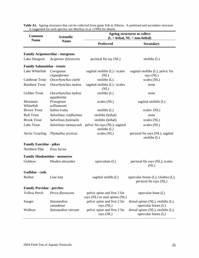
2004 Field Test of Aquatic Protocols 35
Table A1. Ageing structures that can be collected from game fish in Alberta. A preferred and secondary structure is suggested for each species; see MacKay et al. (1990) for details.
Ageing structures to collect (L = lethal, NL = non-lethal) Common
Name
Scientific Name
Preferred Secondary
Family Acipenseridae - sturgeons Lake Sturgeon Acipenser fulvescens pectoral fin ray (NL) otoliths (L)
Family Salmonidae - trouts Lake Whitefish Coregonus
clupeaformis sagittal otoliths (L) / scales
(NL) sagittal otoliths (L), pelvic fin
rays (NL) Cutthroat Trout Oncorhynchus clarki otoliths (L) scales (NL) Rainbow Trout Oncorhynchus mykiss sagittal otoliths (L) / scales
(NL) none
Golden Trout Oncorhynchus mykiss aguabonita
otoliths (L) none
Mountain Whitefish
Prosopium williamsoni
scales (NL) sagittal otoliths (L)
Brown Trout Salmo trutta otoliths (L) scales (NL) Bull Trout Salvelinus confluentus otoliths (lethal) none Brook Trout Salvelinus fontinalis otoliths (lethal) scales (NL) Lake Trout Salvelinus namaycush pelvic fin rays (NL); sagittal
otoliths (L) scales (NL)
Arctic Grayling Thymallus arcticus scales (NL)
pectoral fin rays (NL), sagittal otoliths (L)
Family Esocidae - pikes Northern Pike Esox lucius
Family Hiodontidae - mooneyes Goldeye Hiodon alosoides operculum (L)
pectoral fin rays (NL); scales
(NL)
Gadidae - cods Burbot Lota lota sagittal otolith (L) opercular bones (L), cleithra (L),
pectoral fin rays (NL)
Family Percidae - perches Yellow Perch Perca flavescens pelvic spine and first 2 fin
rays (NL) or anal spines (NL)opercular bone (L)
Sauger Stizostedion canadense
pelvic spine and first 2 fin rays (NL)
dorsal spines (NL), otoliths (L), opercular bones (L)
Walleye Stizostedion vitreum pelvic spine and first 2 fin rays (NL)
dorsal spines (NL), otoliths (L), opercular bones (L)

2004 Field Test of Aquatic Protocols 36
APPENDIX B. REGULATIONS FOR MARKING NETS AND TRAPS. Provincial regulations stipulate that fishing gear must be marked to ensure public safety, and to provide information for individuals encountering the gear. Adequate marking of gear is especially important in lakes with public access, where the number of boaters can be expected to be higher than in more remote locations.
Each end of a gillnet must be marked with a spar buoy, the top of which is at least 1 m above the surface of the water. The buoy must be clearly marked in letters at least 20 mm high with the fish research license number and the name of the research license holder. Each buoy must be marked with a blaze orange or red flag at least 20 x 20 cm in size. The location of minnow traps must be clearly marked using a buoy or other device (e.g. lengths of pool noodle). A weather proof tag at least 5 x 10 cm in size must be affixed to the trap itself; this tag must bear the fish research license number and the name of the license holder, in letters at least 20 mm high. Although pool noodles are adequate for marking the locations of minnow traps, because they lie horizontally in the water they can be difficult to see when waves are present on the water’s surface.